NysAct: A Scalable Preconditioned Gradient Descent using Nyström Approximation

Abstract

Adaptive gradient methods are computationally efficient and converge quickly, but they often suffer from poor generalization. In contrast, second-order methods enhance convergence and generalization but typically incur high computational and memory costs. In this work, we introduce NysAct, a scalable first-order gradient preconditioning method that strikes a balance between state-of-the-art first-order and second-order optimization methods. NysAct leverages an eigenvalue-shifted Nyström method to approximate the activation covariance matrix, which is used as a preconditioning matrix, significantly reducing time and memory complexities with minimal impact on test accuracy. Our experiments show that NysAct not only achieves improved test accuracy compared to both first-order and second-order methods but also demands considerably less computational resources than existing second-order methods. Code is available at https://github.com/hseung88/nysact.

Keywords Deep learning optimization  $\cdot$ Gradient preconditioning  $\cdot$ Nyström approximation

This is the extended version of the paper published in the 2024 IEEE International Conference on Big Data (BigData), © IEEE. The published version is available at: 10.1109/BigData62323.2024.10825352

1 Introduction

The success of deep learning models heavily depends on optimization strategies, with gradient-based methods being crucial for effective training. Gradient preconditioning has gained traction for its ability to accelerate convergence by adjusting gradients during training. First-order methods such as stochastic gradient descent with momentum (SGD) robbins1951Stochastic and Adam(W) kingma2015adam ; Loshchilov2019DecoupledWD are popular for their computational efficiency, with Adam(W) using adaptive learning rates based on the second moments of gradients. However, despite their low per-iteration cost, their convergence is often slow.

Second-order methods can improve the convergence by preconditioning gradients to make them effective in navigating ill-conditioned loss landscapes Gupta2018ShampooPS ; Goldfarb2020PracticalQM ; Liu2024Sophia . However, their computational overhead is often prohibitive, especially in large-scale deep learning tasks. For example, directly leveraging the Hessian matrix Tran2022Better ; frangella2024sketchysgd as a preconditioner requires double backpropagation, significantly increasing time and memory demands. To improve efficiency, methods like KFAC martens2015optimizing approximates the (empirical) Fisher information matrix (FIM), instead of the Hessian, and decompose it into the Kronecker product of smaller matrices but still result in longer training times compared to SGD. For example, in our experiments with ResNet-110 on CIFAR-100 using a single GPU, AdaHessian Yao2020ADAHESSIANAA took on average 46.33 seconds per epoch, Shampoo Gupta2018ShampooPS 200.63 seconds, and KFAC 21.75 seconds, while SGD took only 8.88 seconds.

In this work, we propose a novel stochastic preconditioned optimizer called NysAct, whose performance is as good as that of second-order methods while requiring significantly less computation and memory. KFAC approximates the FIM ${\bm{\mathrm{F}}}\in\mathbb{R}^{mn\times mn}$ of a layer with the Kronecker product of two matrices: ${\bm{\mathrm{F}}}={\bm{\mathrm{A}}}\otimes{\bm{\mathrm{P}}}$, where ${\bm{\mathrm{A}}}\in\mathbb{R}^{n\times n}$ and ${\bm{\mathrm{P}}}\in\mathbb{R}^{m\times m}$ are covariance matrix of activations and pre-activation gradients, respectively. A recent work Benzing2022GradientDO empirically found that the term ${\bm{\mathrm{P}}}$ makes no contribution to the high performance of KFAC and proposed an optimizer, called FOOF, that replaces ${\bm{\mathrm{P}}}$ with an identity matrix ${\bm{\mathrm{I}}}$. Based on this observation, NysAct chooses to use activation covariance matrix as a preconditioner. While only computing and maintaining ${\bm{\mathrm{A}}}$ saves both computation and memory space, FOOF still suffers from low scalability due to the need for complex matrix operations on ${\bm{\mathrm{A}}}$, rendering it impractical for large neural networks.

To improve scalability, NysAct further approximates the activation covariance matrix ${\bm{\mathrm{A}}}$ using the eigenvalue-shifted Nyström method Tropp2017FixedRankAO ; Ray2021SublinearTA . Given a matrix ${\bm{\mathrm{A}}}\in\mathbb{R}^{n\times n}$ and a fixed rank $r\ll n$, the Nyström method requires only $\mathcal{O}(r^{3}+nr^{2})$ time and $\mathcal{O}(nr)$ memory to compute the approximation of ${\bm{\mathrm{A}}}^{-1}$. In contrast, low-rank approximations that use singular value decomposition (SVD) have time and memory complexities of $\mathcal{O}(n^{3})$ and $\mathcal{O}(n^{2})$, respectively. The eigenvalue-shifted Nyström method due to Tropp et al. Tropp2017FixedRankAO is specifically adapted for positive semi-definite matrices and offers a sharp approximation error bound, making it an effective choice for scalable gradient preconditioning in deep learning. We also make an important observation. There are two commonly used sampling methods for Nystöm approximation, uniform column sampling without replacement and Gaussian sketching. In our experiments comparing the efficacy of these two sampling methods for curvature matrix approximation, we observed that both methods perform similarly when the input dataset is small to medium-scale dataset but, when the input is large-scale, the Gaussian sketching method performs worse than the subcolumn sampling method.

To demonstrate the effectiveness of the Nyström method in approximating the activation covariance matrix, we trained ResNet-32 model he2016deep on CIFAR-100 krizhevsky2009learning dataset for 100 epochs using SGD with a mini-batch size of 128. Figure 1 shows the heatmaps of actual and Nyström approximated covariance matrices. As shown, the Nyström method has an ability to recover the whole covariance matrix from the randomly sampled subset of $r$ columns.

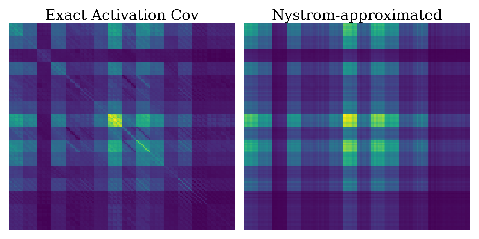
(a) Layer1.2.Conv1

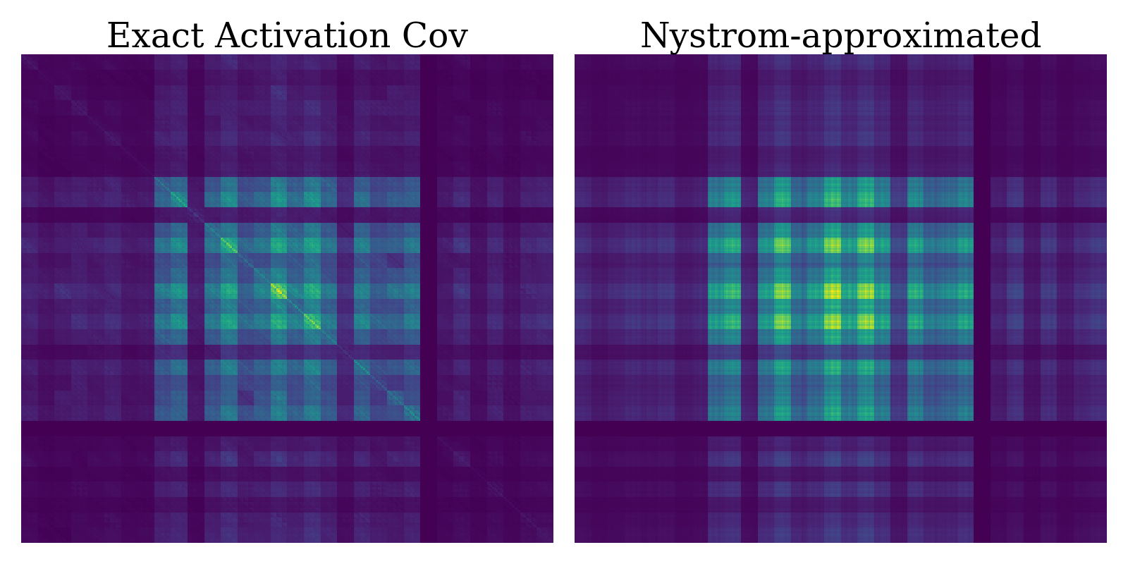
(b) Layer2.1.Conv1

Figure 1: Comparison of exact activation covariance and Nyström-approximated activation covariance in ResNet-32 architecture trained on CIFAR-100 dataset

1.1 Contributions

The key contributions of this paper are summarized as follows.

Scalable Gradient Preconditioning. We introduce NysAct, a scalable gradient preconditioning method that significantly reduces computational costs while maintaining a minimal compromise in performance. By integrating the Nyström approximation with activation covariance, our method strikes a balance between efficiency and accuracy, making it well-suited for large-scale deep learning tasks.

Convergence Analysis. We present a detailed convergence analysis of NysAct, showing that it achieves a convergence rate of $\mathcal{O}(1/T)$, thereby establishing theoretical guarantees for non-convex optimization problems. The analysis highlights how the Nyström approximation impacts the convergence rate, offering valuable insights into the trade-offs between computational efficiency and optimization performance. This theoretical contribution provides a solid foundation for understanding the behavior of NysAct in deep learning applications.

Extensive Experimental Validation. We provide extensive experimental results that demonstrate the effectiveness of NysAct in image classification tasks. Our experiments, conducted across various network architectures on CIFAR and ImageNet datasets, show that NysAct not only achieves higher test accuracy than both state-of-the-art first-order and second-order methods but also requires less time and memory resources compared to second-order methods.

2 Related Work

The work closest to ours is SketchySGD frangella2024sketchysgd which also uses the Nyström method Williams2000UsingTN to obtain a preconditioner. Specifically, it approximates the (minibatch) Hessian with a low-rank matrix using Hessian vector products. However, SketchySGD requires double backpropagation to compute these approximations, leading to substantial memory and time overhead. In our experiments of training ResNet-110 on CIFAR-100 dataset, SketchySGD required an average 58.14 seconds per epoch and used 21.3 GB of memory with a mini-batch size of 128 on a single GPU. In contrast, NysAct took only 11.32 seconds and 1.1 GB of memory. Although SketchySGD is most closely related to NysAct, we excluded it from our baselines due to its unacceptably high resource requirement.

Other notable methods that use a low-rank scalable approximation for preconditioning include GGT Agarwal2020EfficientFA , K-BFGS Goldfarb2020PracticalQM , MFAC frantar2021mfac , SKFAC Tang2021SKFACTN , and Eva Zhang2023EvaPS . GGT exploits the low-rank structure of the sum of the outer product of the gradient and efficiently computes its inverse square root using SVD. While it has lower computational overhead compared to full-matrix preconditioning, it remains resource-intensive because of the need for performing SVD on the matrix formed by past gradients. K-BFGS efficiently computes the inverse of the approximated FIM used in KFAC by employing the BFGS method Broyden1970TheCO ; Fletcher1970ANA ; Goldfarb1970AFO ; Shanno1970ConditioningOQ . However, it requires additional forward and backward passes to compute the $(\bm{\mathrm{s}},\bm{\mathrm{y}})$ pair for BFGS updates, increasing the overall computational cost. MFAC introduced rank-1 approximations for estimating inverse-Hessian vector products, employing iterative conjugate gradient solvers. However, this method necessitates multiple forward and backward passes, which significantly raises both computational and memory requirements. SKFAC proposed a low-rank formulation for the inverse of FIM using the Sherman-Morrison-Woodbury formula. It stores both the activation covariance and pre-activation gradient covariance matrices as used in KFAC, requiring the inversion of both matrices, whereas NysAct stores only sketched activation covariance matrices. Among KFAC’s low-rank approximation variants, Eva is the most efficient method that preserves KFAC’s original performance. Eva computes and stores batch-averaged activation and pre-activation gradient vectors, and updates the inverse of the approximated FIM using the Sherman-Morrison formula. However, as demonstrated in Benzing2022GradientDO , KFAC’s effectiveness as a second-order method is primarily driven by the activation term, rather than the pre-activation gradient term.

3 Preliminaries

3.1 Notations

We use lower-case bold letters for (column) vectors and upper-case bold letters for matrices. ${\bm{\mathrm{I}}}_{m}$ is an $m\times m$ identity matrix. For a matrix ${\bm{\mathrm{M}}}\in\mathbb{R}^{p\times q}$, its vectorization, denoted by $\operatorname{vec}({\bm{\mathrm{M}}})$, is the column vector of size $pq\times 1$ obtained by concatenating columns of ${\bm{\mathrm{M}}}$, i.e., $\operatorname{vec}({\bm{\mathrm{M}}})=\begin{bmatrix}{\bm{\mathrm{M}}}_{*,1}^{\intercal}&{\bm{\mathrm{M}}}_{*,2}^{\intercal}&\cdots&{\bm{\mathrm{M}}}_{*,q}^{\intercal}\end{bmatrix}^{\intercal}\,$, where ${\bm{\mathrm{M}}}_{*,j}$ denotes the $j$^th column of matrix ${\bm{\mathrm{M}}}$. For any matrix ${\bm{\mathrm{M}}}$, we denote the set of its eigenvalues by $\lambda({\bm{\mathrm{M}}})$ and the set of its singular values by $\sigma({\bm{\mathrm{M}}})$, both assumed to be sorted in descending order. The Frobenius norm is denoted by $\|{\bm{\mathrm{M}}}\|_{F}$, and the Kronecker product is represented by $\otimes$. The set $\{1,2,\dots,N\}$ is denoted by $[N]$.

3.2 Setup for Architecture and Training

Consider a network $f(\bm{\mathrm{x}};\bm{\mathrm{\theta}})$ composed of $L$ layers, trained on a dataset $\mathcal{D}=\{(\bm{\mathrm{x}}_{i},y_{i})\}_{i=1}^{n}$. For each layer $l\in[L]$, let ${\bm{\mathrm{W}}}^{(l)}\in\mathbb{R}^{d_{l}\times d_{l-1}}$ represents the weight matrix, and $\bm{\mathrm{b}}^{(l)}\in\mathbb{R}^{d_{l}}$ represents the bias vector. The forward step of $f$ is defined as follows:

$$\bm{\mathrm{z}}^{(l)}={\bm{\mathrm{W}}}^{(l)}\bm{\mathrm{a}}^{(l-1)}+\bm{\mathrm{b}}^{(l)}\in\mathbb{R}^{d_{l}}\,,$$

$$\bm{\mathrm{a}}^{(l)}=\phi(\bm{\mathrm{z}}^{(l)})\in\mathbb{R}^{d_{l}}\,,\qquad\bm{\mathrm{a}}^{(0)}=\bm{\mathrm{x}}\,,$$

$$\bm{\mathrm{\theta}}^{(l)}=[\operatorname{vec}({\bm{\mathrm{W}}}^{(l)})^{\intercal},(\bm{\mathrm{b}}^{(l)})^{\intercal}]^{\intercal}\in\mathbb{R}^{d_{l}(d_{l-1}+1)}\,,$$

$$\bm{\mathrm{\theta}}\in[(\bm{\mathrm{\theta}}^{(1)})^{\intercal},\ldots,(\bm{\mathrm{\theta}}^{(L)})^{\intercal}]^{\intercal}\in\mathbb{R}^{p}\,,$$

where $\bm{\mathrm{z}}$ denotes the pre-activations, $\bm{\mathrm{a}}$ represents the activations, and $\phi$ is the activation function. For convolutional layers, similar to KFAC, we employed patch extraction to unfold the input into patches, transforming the additional axes into a format compatible with matrix operations.

We consider training a deep neural network $f:\mathbb{R}^{d}\to\mathbb{R}$ that takes an input $\bm{\mathrm{x}}$ and produces an output $f(\bm{\mathrm{\theta}};\bm{\mathrm{x}})$. Given training examples $\mathcal{D}$, we aim to learn the network parameters $\bm{\mathrm{\theta}}$ by minimizing the empirical loss $\mathcal{L}$ over the training set:

$$\min_{\bm{\mathrm{\theta}}\in\mathbb{R}^{d}}\mathcal{L}(\bm{\mathrm{\theta}};\mathcal{D}):=\frac{1}{n}\sum_{i=1}^{n}{\ell\left(f(\bm{\mathrm{x}}_{i};\bm{\mathrm{\theta}}),y_{i}\right)},$$ (1)

where $\ell$ is a loss function. Throughout the paper, $\mathcal{B}_{k}$ denotes the minibatch at iteration $k$ constructed by randomly sampling examples in $\mathcal{D}$.

3.3 FIM-based Gradient Preconditioning

To solve the problem (1), KFAC approximates the FIM with a Kronecker product of smaller matrices as ${\bm{\mathrm{F}}}^{(l)}\approx{\bm{\mathrm{A}}}^{(l-1)}\otimes{\bm{\mathrm{P}}}^{(l)}$, where ${\bm{\mathrm{A}}}^{(l)}=\operatorname{\mathbb{E}}\left[\bm{\mathrm{a}}^{(l)}(\bm{\mathrm{a}}^{(l)})^{\intercal}\right]$ denotes the activation covariance from layer $l$, and ${\bm{\mathrm{P}}}^{(l)}=\operatorname{\mathbb{E}}\left[\frac{\partial\mathcal{L}}{\partial\bm{\mathrm{z}}^{(l)}}\frac{\partial\mathcal{L}}{\partial\bm{\mathrm{z}}^{(l)}}^{\intercal}\right]$ represents the pre-activation gradient covariance from layer $l$.

Assuming the independence between layer $i$ and $j$ for $i\neq j$, KFAC computes the diagonal blocks of FIM only, which results in the following update rule for layer $l$ at iteration $k$.

$$\bm{\mathrm{\theta}}_{k+1}^{(l)} =\bm{\mathrm{\theta}}_{k}^{(l)}-\eta_{k}({\bm{\mathrm{A}}}_{k}^{(l-1)}\otimes{\bm{\mathrm{P}}}_{k}^{(l)})^{-1}\bm{\mathrm{g}}_{k}^{(l)}$$

$$=\bm{\mathrm{\theta}}_{k}^{(l)}-\eta_{k}\operatorname{vec}{\left(({\bm{\mathrm{P}}}_{k}^{(l)})^{-1}{\bm{\mathrm{G}}}_{k}^{(l)}({\bm{\mathrm{A}}}_{k}^{(l-1)})^{-1}\right)}\,,$$ (2)

where ${\bm{\mathrm{G}}}$ represents the gradient of the loss with respect to the parameters, and $\bm{\mathrm{g}}$ denotes the gradient in vectorized form. A notable scalable KFAC variant recently proposed is Eva which has following update rule:

$$\bm{\mathrm{\theta}}_{k+1}^{(l)} =\bm{\mathrm{\theta}}_{k}^{(l)}-\eta_{k}\operatorname{vec}{\left((\tilde{{\bm{\mathrm{P}}}}_{k}^{(l)})^{-1}{\bm{\mathrm{G}}}_{k}^{(l)}(\tilde{{\bm{\mathrm{A}}}}_{k}^{(l-1)})^{-1}\right)}\,,$$

where the matrix $\tilde{{\bm{\mathrm{A}}}}$ is defined as $\tilde{{\bm{\mathrm{A}}}}=\operatorname{\mathbb{E}}\left[\bm{\mathrm{a}}^{(l-1)}\right]\operatorname{\mathbb{E}}\left[\bm{\mathrm{a}}^{(l-1)}\right]^{\intercal}$ and the matrix $\tilde{{\bm{\mathrm{P}}}}$ is given by $\tilde{{\bm{\mathrm{P}}}}=\operatorname{\mathbb{E}}\left[\frac{\partial\mathcal{L}}{\partial\bm{\mathrm{z}}^{(l)}}\right]\operatorname{\mathbb{E}}\left[\frac{\partial\mathcal{L}}{\partial\bm{\mathrm{z}}^{(l)}}\right]^{\intercal}$. The update rule for FOOF is given by substituting ${\bm{\mathrm{P}}}$ in (3.3) into the identity matrix ${\bm{\mathrm{I}}}$:

$$\bm{\mathrm{\theta}}_{k+1}^{(l)}=\bm{\mathrm{\theta}}_{k}^{(l)}-\eta_{k}\operatorname{vec}{\left({\bm{\mathrm{G}}}_{k}^{(l)}({\bm{\mathrm{A}}}_{k}^{(l-1)})^{-1}\right)}\,.$$

3.4 Nyström Method

The Nyström method Williams2000UsingTN is a well-established technique for constructing low-rank approximations of a matrix ${\bm{\mathrm{A}}}\in\mathbb{R}^{n\times n}$ by selecting a subset of its columns. Specifically, let ${\bm{\mathrm{S}}}\in\mathbb{R}^{n\times r}$ be a matrix that randomly samples $r\ll n$ columns of ${\bm{\mathrm{A}}}$, where each column of ${\bm{\mathrm{S}}}$ is a vector having one entry equal to 1 and all other entries are 0. Then ${\bm{\mathrm{A}}}{\bm{\mathrm{S}}}\in\mathbb{R}^{n\times r}$ corresponds to the submatrix of ${\bm{\mathrm{A}}}$ formed by $r$ randomly sampled columns of ${\bm{\mathrm{A}}}$. The Nyström approximation ${\bm{\mathrm{A}}}_{\text{nys}}$ of ${\bm{\mathrm{A}}}$ is given by

$${\bm{\mathrm{A}}}\approx{\bm{\mathrm{A}}}_{\text{nys}}={\bm{\mathrm{A}}}{\bm{\mathrm{S}}}{\bm{\mathrm{(}}}{\bm{\mathrm{S}}}^{\intercal}{\bm{\mathrm{A}}}{\bm{\mathrm{S}}})^{\dagger}{\bm{\mathrm{S}}}^{\intercal}{\bm{\mathrm{A}}}\,,$$

where ${\bm{\mathrm{X}}}^{\dagger}$ denotes the Moore-Penrose pseudoinverse. Notice that ${\bm{\mathrm{A}}}_{\text{nys}}$ can be obtained by storing ${\bm{\mathrm{S}}}^{\intercal}{\bm{\mathrm{A}}}{\bm{\mathrm{S}}}\in\mathbb{R}^{r\times r}$ and ${\bm{\mathrm{A}}}{\bm{\mathrm{S}}}\in\mathbb{R}^{n\times r}$, which only takes $\mathcal{O}(nr)$ memory space.

There are alternative ways of constructing the sampling matrix ${\bm{\mathrm{S}}}$. One way is to sample each entry of ${\bm{\mathrm{S}}}$ from the standard Guassian distribution $\mathcal{N}(0,1)$, which is called Gaussian sketching. Instead of sampling columns, the Gaussian sketching randomly projects the points in ${\bm{\mathrm{A}}}$ onto a lower dimensional space.

4 Algorithm

In this section, we describe the details of each step in the proposed NysAct algorithm. The pseudocode is provided in Algorithm 1.

Algorithm 1 NysAct

Require: Learning rate $\eta_{k}$, Momentum $\beta_{1}$, EMA $\beta_{2}$, Damping $\rho$, Covariance update frequency $\tau_{cov}$, Inverse update frequency $\tau_{inv}$, Rank $r$
Initialize: Parameter $\bm{\mathrm{\theta}}_{0}^{(l)}$, Momentum vectors $\bm{\mathrm{m}}_{0}^{(l)}=\bm{\mathrm{0}}$, Sketching matrices $\tilde{{\bm{\mathrm{C}}}}_{0}^{(l)}={\bm{\mathrm{O}}}$, Preconditioning matrices $({\bm{\mathrm{C}}}_{0,\text{nys}}^{(l)})^{-1}={\bm{\mathrm{I}}}$

1: for $k=1,2,3,\dots$ do

2:  Construct minibatch $\mathcal{B}_{k}$ by randomly sampling from $\mathcal{D}$

3:  if Sketch == "Gaussian" then

4:   ${\bm{\mathrm{S}}}^{(l)}=(S_{ij})_{1\leq i\leq d_{l-1},\,1\leq j\leq r},\,S_{ij}\sim\mathcal{N}(0,\frac{1}{d_{l-1}})$

5:  else if Sketch == "Subcolumn" then

6:   Indices = RandPerm$(d_{l-1})[:r]$

7:   ${\bm{\mathrm{S}}}^{(l)}={\bm{\mathrm{I}}}_{d_{l-1}}{[\text{Indices}]}\in\mathbb{R}^{d_{l-1}\times r}$

8:  if $(k\mod\tau_{cov})=0$ then

9:   $\widetilde{{\bm{\mathrm{C}}}}_{k}^{(l)}=\beta_{2}\cdot\widetilde{{\bm{\mathrm{C}}}}_{k-1}^{(l)}+(1-\beta_{2})\cdot{\bm{\mathrm{A}}}_{k}^{(l)}{\bm{\mathrm{S}}}^{(l)}\in\mathbb{R}^{d_{l-1}\times r}$

10:  if $(k\mod\tau_{inv})=0$ then

11:   $\widehat{{\bm{\mathrm{C}}}}_{k}^{(l)}=\widetilde{{\bm{\mathrm{C}}}}_{k}^{(l)}/(1-\beta_{2}^{\lfloor k/\tau_{cov}\rfloor})$

12:   $\widehat{{\bm{\mathrm{C}}}}_{k,\text{damped}}^{(l)}=\widehat{{\bm{\mathrm{C}}}}_{k}^{(l)}+\rho\cdot{\bm{\mathrm{S}}}^{(l)}$

13:   ${\bm{\mathrm{W}}}^{(l)}=({\bm{\mathrm{S}}}^{(l)})^{\intercal}\widehat{{\bm{\mathrm{C}}}}_{k,\text{damped}}^{(l)}\in\mathbb{R}^{r\times r}$

14:   Eigendecomposition: ${\bm{\mathrm{W}}}^{(l)}={\bm{\mathrm{Q}}}{\bm{\mathrm{\Lambda}}}{\bm{\mathrm{Q}}}^{\intercal}$

15:   ${\bm{\mathrm{W}}}_{\text{shifted}}^{(l)}={\bm{\mathrm{Q}}}\left[{\bm{\mathrm{\Lambda}}}+\left(|\lambda_{\min}({\bm{\mathrm{W}}}^{(l)})|+\rho\right){\bm{\mathrm{I}}}\right]{\bm{\mathrm{Q}}}^{\intercal}$

16:   Cholesky decomposition: ${\bm{\mathrm{W}}}_{\text{shifted}}^{(l)}={\bm{\mathrm{R}}}^{\intercal}{\bm{\mathrm{R}}}$

17:   ${\bm{\mathrm{X}}}^{(l)}=\widehat{{\bm{\mathrm{C}}}}_{k,\text{damped}}^{(l)}{\bm{\mathrm{R}}}^{-1}\in\mathbb{R}^{d_{l-1}\times r}$

18:   Singular value decomposition: ${\bm{\mathrm{X}}}^{(l)}={\bm{\mathrm{U}}}{\bm{\mathrm{\Sigma}}}{\bm{\mathrm{V}}}^{\intercal}$

19:   $\widetilde{{\bm{\mathrm{\Sigma}}}}=\operatorname{diag}\left(\max\left(\bm{\mathrm{\sigma}}^{2}-(|\lambda_{\min}({\bm{\mathrm{W}}}^{(l)})|+\rho)\bm{\mathrm{1}}_{r},\bm{\mathrm{0}}_{r}\right)\right)$  $\in\mathbb{R}^{r\times r}$

20:   $({\bm{\mathrm{C}}}_{k,\text{nys}}^{(l)})^{-1}={\bm{\mathrm{U}}}_{[:r]}\widetilde{{\bm{\mathrm{\Sigma}}}}^{-1}{\bm{\mathrm{U}}}_{[:r]}^{\intercal}+\frac{1}{\rho}({\bm{\mathrm{I}}}-{\bm{\mathrm{U}}}_{[:r]}{\bm{\mathrm{U}}}_{[:r]}^{\intercal})$     $\in\mathbb{R}^{d_{l-1}\times d_{l-1}}$

21:  ${\bm{\mathrm{G}}}_{k}=\nabla\mathcal{L}(\bm{\mathrm{\theta}}_{k})\in\mathbb{R}^{d_{l}\times d_{l-1}}$

22:  $\bm{\mathrm{m}}_{k}^{(l)}=\beta_{1}\bm{\mathrm{m}}_{k-1}^{(l)}-\eta_{k}\operatorname{vec}{\left({\bm{\mathrm{G}}}_{k}^{(l)}({\bm{\mathrm{C}}}_{k,\text{nys}}^{(l)})^{-1}\right)}$

23:  $\bm{\mathrm{\theta}}_{k}^{(l)}=\bm{\mathrm{\theta}}_{k-1}^{(l)}+\bm{\mathrm{m}}_{k}^{(l)}$

At iteration $k$, the algorithm estimates the covariance ${\bm{\mathrm{A}}}_{k}^{(l)}$ of activations $\bm{\mathrm{a}}^{(l)}$ for each layer $l$ using the examples in the minibatch $\mathcal{B}_{k}$:

$${\bm{\mathrm{A}}}_{k}^{(l)}=\operatorname{\mathbb{E}}\left[\bm{\mathrm{a}}^{(l)}\left(\bm{\mathrm{a}}^{(l)}\right)^{\intercal}\right]\approx\frac{1}{|\mathcal{B}_{k}|}\sum_{i\in\mathcal{B}_{k}}\bm{\mathrm{a}}_{i}^{(l)}(\bm{\mathrm{a}}_{i}^{(l)})^{\intercal}\,,$$

where $\bm{\mathrm{a}}_{i}^{(l)}$ denotes the activations of network $f(\bm{\mathrm{x}}_{i};\bm{\mathrm{\theta}}_{k})$ at layer $l$. Let ${\bm{\mathrm{G}}}_{k}^{(l)}=\nabla_{\bm{\mathrm{\theta}}^{(l)}}\mathcal{L}(\bm{\mathrm{\theta}}_{k};\mathcal{B}_{k})\in\mathbb{R}^{d_{l}\times d_{l-1}}$ be the minibatch-estimated gradient of layer $l$ with input and output dimensions $d_{\text{in}}=d_{l-1}$ and $d_{\text{out}}=d_{l}$, respectively. FOOF updates the parameters of layer $l$ as follows:

$$\bm{\mathrm{\theta}}_{k+1}^{(l)} =\bm{\mathrm{\theta}}_{k}^{(l)}-\eta_{k}({\bm{\mathrm{C}}}_{k}^{(l)}\otimes{\bm{\mathrm{I}}}_{d_{l}})^{-1}\operatorname{vec}({\bm{\mathrm{G}}}_{l}^{(l)})$$

$$=\bm{\mathrm{\theta}}_{k}^{(l)}-\eta_{k}\operatorname{vec}\left({\bm{\mathrm{G}}}_{k}^{(l)}({\bm{\mathrm{C}}}_{k}^{(l)})^{-1}\right)\,,$$

where ${\bm{\mathrm{C}}}_{k}^{(l)}$ is the exponential moving average (EMA) of covariance matrix of activations of $l-1$, given by

$${\bm{\mathrm{C}}}_{k}^{(l)}=\beta_{2}{\bm{\mathrm{C}}}_{k-1}^{(l)}+(1-\beta_{2}){\bm{\mathrm{A}}}_{k}^{(l-1)}\in\mathbb{R}^{d_{\text{in}}\times d_{\text{in}}}\,.$$ (3)

Compared to KFAC update in (3.3), the update in (3) only requires computing and storing the EMA of ${\bm{\mathrm{A}}}_{k}^{(l)}$, which reduces time and memory complexity from $\mathcal{O}(d_{\text{out}}^{3}+d_{\text{in}}^{3})$ to $\mathcal{O}(d_{\text{in}}^{3})$ and from $\mathcal{O}(d_{\text{out}}^{2}+d_{\text{in}}^{2})$ to $\mathcal{O}(d_{\text{in}}^{2})$, respectively. However, for large-scale networks, $\mathcal{O}(d_{\text{in}}^{3})$ can still be prohibitively expensive. To mitigate the issue, we propose to obtain a randomized low-rank approximation ${\bm{\mathrm{C}}}_{k,\text{nys}}^{(l)}$ of ${\bm{\mathrm{C}}}_{k}^{(l)}$ using the Nyström method.

4.1 Eigenvalue-shifted Nyström

Let ${\bm{\mathrm{S}}}_{k}^{(l)}\in\mathbb{R}^{d_{\text{in}}\times r}$ be a sampling matrix such that ${\bm{\mathrm{A}}}_{k}^{(l)}{\bm{\mathrm{S}}}_{k}^{(l)}$ is a random subset of $r$ columns from ${\bm{\mathrm{A}}}_{k}^{(l)}$ (line 7) or a Gaussian sketching of ${\bm{\mathrm{A}}}_{k}^{(l)}$ (line 4). We call our method NysAct-S when ${\bm{\mathrm{S}}}_{k}^{(l)}$ samples the columns and NysAct-G when ${\bm{\mathrm{S}}}_{k}^{(l)}$ performs Gaussian sketching. Instead of storing ${\bm{\mathrm{A}}}_{k}^{(l)}\in\mathbb{R}^{d_{\text{in}}\times d_{\text{in}}}$, NysAct maintains EMA of ${\bm{\mathrm{A}}}_{k}^{(l)}{\bm{\mathrm{S}}}_{k}^{(l)}\in\mathbb{R}^{d_{\text{in}}\times r}$, which modifies the EMA update in (3) as follows:

$$\widetilde{{\bm{\mathrm{C}}}}_{k}^{(l)}=\beta_{2}\widetilde{{\bm{\mathrm{C}}}}_{k-1}^{(l)}+(1-\beta_{2}){\bm{\mathrm{A}}}_{k}^{(l-1)}{\bm{\mathrm{S}}}_{k}^{(l)}\,.$$ (4)

This greatly reduces the memory complexity to $\mathcal{O}(d_{\text{in}}\cdot r)$, where the rank $r$ is normally much smaller than the layer’s input size $d_{\text{in}}$. In our experiments on CIFAR datasets, we set $r=10$. In line 12, to ensure the positive semi-definiteness ${\bm{\mathrm{C}}}_{k}^{(l)}$, NysAct computes the sketch of damped ${\bm{\mathrm{A}}}_{k}^{(l)}$ after applying the bias correction (line 11) to $\widetilde{{\bm{\mathrm{C}}}}_{k}^{(l)}$:

$$\widehat{{\bm{\mathrm{C}}}}_{k,\text{damped}}^{(l)}=\widehat{{\bm{\mathrm{C}}}}_{k}^{(l)}+\rho{\bm{\mathrm{S}}}_{k}^{(l)}\approx({\bm{\mathrm{A}}}_{k}^{(l-1)}+\rho{\bm{\mathrm{I}}}_{d_{l-1}}){\bm{\mathrm{S}}}_{k}^{(l)}\,,$$

where $\rho>0$ is a damping factor.

For clarity, hereafter we omit the layer index $(l)$. Our goal is to obtain the inverse of (damped) activation covariance matrix ${\bm{\mathrm{C}}}_{k}$ from the Nyström sketch $\widetilde{{\bm{\mathrm{C}}}}_{k}$. One can use the standard Nyström method Williams2000UsingTN along with the matrix inversion lemma.

$${\bm{\mathrm{C}}}_{k}^{-1} \approx\left(\rho{\bm{\mathrm{I}}}_{d_{l-1}}+\widetilde{{\bm{\mathrm{C}}}}_{k}({\bm{\mathrm{S}}}_{k}^{\intercal}\widetilde{{\bm{\mathrm{C}}}}_{k})^{\dagger}\widetilde{{\bm{\mathrm{C}}}}_{k}^{\intercal}\right)^{-1}$$

$$=\frac{1}{\rho}{\bm{\mathrm{I}}}_{d_{l-1}}-\frac{1}{\rho^{2}}\widetilde{{\bm{\mathrm{C}}}}_{k}\left({\bm{\mathrm{S}}}_{k}^{\intercal}\widetilde{{\bm{\mathrm{C}}}}_{k}+\frac{1}{\rho}\widetilde{{\bm{\mathrm{C}}}}_{k}^{\intercal}\widetilde{{\bm{\mathrm{C}}}}_{k}\right)^{-1}\widetilde{{\bm{\mathrm{C}}}}_{k}^{\intercal}$$ (5)

However, the above equation is not numerically stable frangella2023Randomized ; Goldfarb2020PracticalQM . We also empirically observed that computing the inverse using (5) results in training instability. Instead, we propose to use the numerically stable eigenvalue-shifted Nyström method Tropp2017FixedRankAO ; Ray2021SublinearTA . The low-rank approximation procedure presented in Algorithm 1 combines the ideas of Tropp2017FixedRankAO and Ray2021SublinearTA and adapt it to deep learning settings. To obtain a rank-$r$ approximation $\widehat{{\bm{\mathrm{C}}}}_{k,\text{nys}}$ of ${\bm{\mathrm{C}}}_{k}+\rho{\bm{\mathrm{I}}}_{d_{\text{in}}}$, NysAct computes the Cholesky decomposition ${\bm{\mathrm{S}}}_{k}^{\intercal}\widehat{{\bm{\mathrm{C}}}}_{k,\text{damped}}={\bm{\mathrm{R}}}^{\intercal}{\bm{\mathrm{R}}}\in\mathbb{R}^{r\times r}$ in line 16, which allows to express

$$\widehat{{\bm{\mathrm{C}}}}_{k,\text{nys}} =\widehat{{\bm{\mathrm{C}}}}_{k,\text{damped}}({\bm{\mathrm{S}}}_{k}^{\intercal}\widehat{{\bm{\mathrm{C}}}}_{k,\text{damped}})^{-1}\widehat{{\bm{\mathrm{C}}}}_{k,\text{damped}}$$

$$=(\widehat{{\bm{\mathrm{C}}}}_{k,\text{damped}}{\bm{\mathrm{R}}}^{-1})(\widehat{{\bm{\mathrm{C}}}}_{k,\text{damped}}{\bm{\mathrm{R}}}^{-1})^{\intercal}={\bm{\mathrm{X}}}{\bm{\mathrm{X}}}^{\intercal}\,.$$

Let the eigenvalue decomposition of ${\bm{\mathrm{X}}}$ be given by ${\bm{\mathrm{X}}}={\bm{\mathrm{U}}}{\bm{\mathrm{\Sigma}}}{\bm{\mathrm{V}}}^{\intercal}$. Then we have $\widehat{{\bm{\mathrm{C}}}}_{\text{nys}}={\bm{\mathrm{U}}}{\bm{\mathrm{\Sigma}}}^{2}{\bm{\mathrm{U}}}^{\intercal}$ and its inverse $\widehat{{\bm{\mathrm{C}}}}_{k,\text{nys}}^{-1}$ can be easily obtained by replacing the diagonal elements of ${\bm{\mathrm{\Sigma}}}^{2}$ by their reciprocals (line 20). For numerical stability of linear algebraic operations that requires positve-definite matrices, line 15 shifts the eigenvalues of ${\bm{\mathrm{W}}}$ and they are shifted back in line 19 to remove the effect of the shift..

Table 1: Comparison of time and memory complexity for updating preconditioner(s)

Method	Time Complexity	Memory Complexity
KFAC	$\mathcal{O}(d_{\text{out}}^{3})+\mathcal{O}(d_{\text{in}}^{3})$	$\mathcal{O}(d_{\text{out}}^{2})+\mathcal{O}(d_{\text{in}}^{2})$
Eva	$\mathcal{O}(d_{\text{out}}^{2})+\mathcal{O}(d_{\text{in}}^{2})$	$\mathcal{O}(d_{\text{out}})+\mathcal{O}(d_{\text{in}})$
FOOF	$\mathcal{O}(d_{\text{in}}^{3})$	$\mathcal{O}(d_{\text{in}}^{2})$
NysAct	$\mathcal{O}(r^{3})+\mathcal{O}(d_{\text{in}}\cdot r^{2})$	$\mathcal{O}(d_{\text{in}}\cdot r)$

4.2 Complexities

We compare the asymptotic time and memory costs of preconditioning a layer with a weight matrix of size $(d_{\text{out}}\times d_{\text{in}})$ in Table 1. The most computationally intensive steps in NysAct occur in Line 14, 16, 17, and 18. However, since the rank $r$ is typically much smaller than the dimensions of the weight matrix, NysAct is expected to have significantly lower complexity than KFAC and FOOF, making it more scalable and suitable for large-scale deep learning tasks.

4.3 Hyperparameters

NysAct is robust to variations in the learning rate $\eta$, EMA coefficient $\beta_{2}$, damping factor $\rho$, and inverse update frequency $\tau_{inv}$, allowing for consistent and reliable performance with less effort in hyperparameter tuning. In our experiments, we observed that NysAct, FOOF, and other KFAC variants perform well when using the same hyperparameters as SGD, such as the learning rate, momentum coefficient $\beta_{1}$, and weight decay.

5 Convergence Analysis

In this section, we analyze the convergence properties of NysAct. To simplify the analysis, we focus on feed-forward networks composed of linear layers, though these results can easily be extended to other types of layers as well. We make the following common standard assumptions in stochastic optimization.

Assumption 5.1 (Smoothness).

The loss function $\mathcal{L}$ is continuously differentiable and $L$-smooth, i.e., for all ${\bm{\mathrm{W}}}_{1},{\bm{\mathrm{W}}}_{2}\in\mathbb{R}^{m\times n}$,

$$\|\nabla\mathcal{L}({\bm{\mathrm{W}}}_{1})-\nabla\mathcal{L}({\bm{\mathrm{W}}}_{2})\|_{F}\leq L\|{\bm{\mathrm{W}}}_{1}-{\bm{\mathrm{W}}}_{2}\|_{F}$$

Assumption 5.2 (Gradient properties).

We make the following assumptions about the stochastic gradient ${\bm{\mathrm{G}}}({\bm{\mathrm{W}}})$:

1. ${\bm{\mathrm{G}}}({\bm{\mathrm{W}}})$ is an unbiased estimate of the true gradient $\nabla{\mathcal{L}}({\bm{\mathrm{W}}})$, i.e.,

   $$\operatorname{\mathbb{E}}[{\bm{\mathrm{G}}}({\bm{\mathrm{W}}})]=\nabla\mathcal{L}({\bm{\mathrm{W}}}).$$

2. The variance of ${\bm{\mathrm{G}}}(W)$ is bounded by $\sigma^{2}>0$:

   $$\operatorname{\mathbb{E}}\left[\|{\bm{\mathrm{G}}}({\bm{\mathrm{W}}})-\nabla\mathcal{L}({\bm{\mathrm{W}}})\|_{F}^{2}\right]\leq\sigma^{2}.$$

3. The second moment of the true gradient is bounded by a constant $C$:

   $$\operatorname{\mathbb{E}}\left[\|\nabla\mathcal{L}({\bm{\mathrm{W}}})\|_{F}^{2}\right]\leq C.$$

Further, we make the following assumptions to guarantee that the activation covariance matrix remains well bounded and the Nyström approximation error is properly controlled.

Assumption 5.3 (Bounded Activation Covariance).

The Frobenius norm of activation covariance ${\bm{\mathrm{A}}}\in\mathbb{R}^{d_{\text{in}}\times d_{\text{in}}}$ is bounded by constants $0<\nu_{L}<\nu_{U}$, such that

$$\nu_{L}\leq\|{\bm{\mathrm{A}}}\|_{F}\leq\nu_{U}.$$

Also, the eigenvalues of ${\bm{\mathrm{A}}}$ are bounded by constants $0<\lambda_{L}<\lambda_{U}$, such that, for all $i\in[d_{\text{in}}]$ and $\mathcal{B}\subset\mathcal{D}$,

$$\lambda_{L}<\lambda_{i}({\bm{\mathrm{A}}}_{\mathcal{B}})<\lambda_{U}.$$

Assumption 5.4 (Nyström Approximation).

The Nyström approximated activation covariance ${\bm{\mathrm{A}}}_{nys}$ of the exact activation covariance ${\bm{\mathrm{A}}}$ satisfies the approximation bound

$$\|{\bm{\mathrm{A}}}-{\bm{\mathrm{A}}}_{nys}\|_{F}\leq\epsilon\|{\bm{\mathrm{A}}}\|_{F}$$

for some small approximation error $\epsilon>0$.

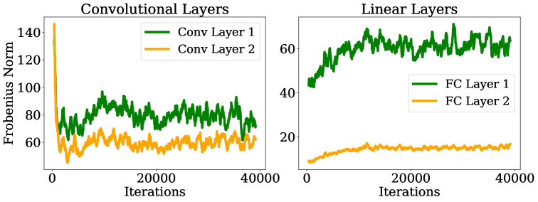
Figure 2: Trajectories of the Frobenius norm of the activation covariance for LeNet-5 layers on CIFAR-10 for 100 epochs.

In support of Assumption 5.3, empirical observations indicate that the Frobenius norm of the activation covariance consistently exhibits natural lower and upper bounds across layers. Figure 2 provides a toy example illustrating the change of the Frobenius norm of the activation covariance at each layer during the training. We trained LeNet-5 lecun98lenet5 on CIFAR-10 dataset using SGD for 100 epochs. The left subplot shows the Frobenius norms for the convolutional layers, while the right subplot shows the Frobenius norms for the fully connected layers. The norms are tracked across training iterations. The result suggests that the assumption of a bounded activation covariance norm is well-founded.

Theorem 5.5 (Convergence of NysAct).

If the learning rate $\eta$ is set as $\eta=\mathcal{O}\left(\frac{(\lambda_{L}-\epsilon\nu_{L}+\rho)^{2}}{\sigma^{2}L(\lambda_{U}+\epsilon\nu_{U}+\rho)}\right)$, then after $T$ iterations, the squared norm of gradient satisfies:

$$\frac{1}{T}\sum_{k=0}^{T-1} {\|\nabla\mathcal{L}({\bm{\mathrm{W}}}_{k})\|_{F}^{2}}\leq\frac{\operatorname{\mathbb{E}}\mathcal{L}({\bm{\mathrm{W}}}_{0})-\operatorname{\mathbb{E}}\mathcal{L}({\bm{\mathrm{W}}}^{*})}{\eta T\left(\frac{1}{\lambda_{U}+\epsilon\nu_{U}+\rho}-\frac{\eta L}{2(\lambda_{L}-\epsilon\nu_{L}+\rho)^{2}}\right)}$$

$$+\frac{\eta\sigma^{2}L}{2(\lambda_{L}-\epsilon\nu_{L}+\rho)^{2}-\eta L(\lambda_{U}+\epsilon\nu_{U}+\rho)}\,,$$ (6)

where $\mathcal{L}({\bm{\mathrm{W}}}^{*})$ denotes the global minimum of the loss function.

Theorem 5.5 indicates that the convergence rate of NysAct is given by $\mathcal{O}(1/T)$. See Appendix A for the proof.

Remark 5.6.

The convergence analysis in (6) demonstrates that the Nyström approximation error $\epsilon$ directly impacts the convergence rate of NysAct. As the approximation error increases, convergence becomes slower, and conversely, reducing the approximation error accelerates convergence. Therefore, a crucial factor for achieving faster convergence lies in effectively controlling and minimizing the approximation error.

6 Experiments

We assess the performance of NysAct on a range of image classification tasks and compare it with other baseline methods. All experiments were conducted using 2 Nvidia RTX6000 GPUs.

Table 2: Test accuracy (%) of ResNet and DenseNet on CIFAR datasets

Dataset	Model	ResNet-32		ResNet-110		DenseNet-121
	Epoch	100	200	100	200	100	200
CIFAR-10	SGD	92.80$\pm$0.21	93.57$\pm$0.29	93.30$\pm$0.24	94.18$\pm$0.43	95.33$\pm$0.16	95.58$\pm$0.13
	Adam	91.59$\pm$0.09	92.28$\pm$0.14	92.43$\pm$0.08	92.90$\pm$0.21	93.11$\pm$0.19	93.35$\pm$0.16
	AdamW	90.79$\pm$0.16	91.83$\pm$0.28	92.33$\pm$0.25	93.19$\pm$0.19	94.24$\pm$0.10	94.56$\pm$0.14
	KFAC	93.16$\pm$0.17	93.78$\pm$0.13	94.35$\pm$0.13	94.64$\pm$0.10	95.23$\pm$0.16	95.57$\pm$0.07
	Eva	93.07$\pm$0.16	93.65$\pm$0.14	94.18$\pm$0.10	94.64$\pm$0.09	95.30$\pm$0.13	95.69$\pm$0.11
	FOOF	93.61$\pm$0.14†	94.05$\pm$0.17†	94.70$\pm$0.10†	95.09$\pm$0.10†	95.79$\pm$0.04†	95.95$\pm$0.08†
	NysAct-g	93.12$\pm$0.11	93.68$\pm$0.21	94.48$\pm$0.09	94.76$\pm$0.12	95.53$\pm$0.13	95.74$\pm$0.10
	NysAct-s	93.28$\pm$0.21‡	93.79$\pm$0.22‡	94.53$\pm$0.17‡	94.94$\pm$0.16‡	95.60$\pm$0.19‡	95.83$\pm$0.08‡
CIFAR-100	SGD	70.47$\pm$0.38	70.67$\pm$0.49	71.44$\pm$1.90	72.48$\pm$1.36	79.63$\pm$0.15	80.32$\pm$0.24
	Adam	67.16$\pm$0.41	67.90$\pm$0.55	70.10$\pm$0.45	71.22$\pm$0.44	73.48$\pm$0.41	73.49$\pm$0.21
	AdamW	65.23$\pm$0.16	67.04$\pm$1.08	68.88$\pm$0.31	70.59$\pm$0.37	75.51$\pm$0.23	76.30$\pm$0.12
	KFAC	70.21$\pm$0.34	70.91$\pm$0.28	73.10$\pm$0.41	74.68$\pm$0.33	79.79$\pm$0.24	80.16$\pm$0.10
	Eva	70.32$\pm$0.31	71.11$\pm$0.50	73.55$\pm$0.33	74.13$\pm$0.34	79.32$\pm$0.08	79.89$\pm$0.27
	FOOF	71.21$\pm$0.34†	71.82$\pm$0.23†	75.13$\pm$0.26†	75.91$\pm$0.31†	80.92$\pm$0.28†	80.98$\pm$0.25†
	NysAct-g	70.70$\pm$0.18	71.14$\pm$0.17‡	73.94$\pm$0.38‡	74.70$\pm$0.19	80.40$\pm$0.24‡	80.70$\pm$0.34‡
	NysAct-s	70.86$\pm$0.44‡	71.12$\pm$0.34	73.76$\pm$0.45	75.01$\pm$0.16‡	80.33$\pm$0.29	80.54$\pm$0.17

• $\dagger$ and $\ddagger$ indicate the best and second-best test accuracies, respectively.

Figure 3: Comparison of training loss and test accuracy of optimizers on CIFAR-100 dataset using (Left) ResNet-110 and (Right) DenseNet-121.

6.1 CIFAR Dataset

Settings. For the CIFAR datasets, we employed ResNet-32, ResNet-110, and DenseNet-121 Huang2016DenselyCC , training each model for 100 and 200 epochs. We used a mini-batch size of 128 and cosine annealing learning rate scheduling Loshchilov2016SGDRSG . The reported metrics in this section are averaged over 5 independent runs. We compared NysAct against state-of-the-art first- and second-order optimization methods. Specifically, we include SGD (with momentum) as an essential baseline and Adam and AdamW as adaptive first-order methods that precondition gradients using their second moments. We evaluate KFAC and Eva as second-order methods that precondition gradients using approximated FIM. Finally, we include FOOF and NysAct as first-order methods that employ activation covariance-based gradient preconditioning.

Training Results. The training results overall indicate that NysAct retains much of FOOF’s strong performance with minimal compromise. As shown in Tables 2, NysAct outperforms most other baselines in terms of test accuracy. While Adam and AdamW exhibit faster convergence during the early stages of training, they ultimately achieve lower test accuracy (i.e., relatively poor generalization performance) compared to other methods. Second-order methods generally outperform the first-order methods, such as SGD, Adam, and AdamW. However, they show less effective performance in both convergence rate and generalization compared to the activation covariance-based preconditioning methods, FOOF and NysAct. When comparing NysAct to FOOF, FOOF delivered the strongest results overall, with NysAct following closely as a strong second. Given that NysAct is designed as a scalable alternative to FOOF, this outcome suggests that its approximation of the activation covariance matrix is reasonably effective. In comparison to KFAC and Eva, NysAct either matches or exceeds their performance in CIFAR-10 training, and it distinctly outperforms all other methods in CIFAR-100 training across all network architectures tested. Figure 3 shows the progression of training loss and test accuracy over 200 epochs on CIFAR-100 dataset. The results for ResNets clearly demonstrate that NysAct effectively balances the fast convergence of first-order methods with the strong generalization capabilities of second-order methods. For DenseNet-121, NysAct performs comparably to the other second-order baselines.

Table 3: Comparison of relative wall-clock time and memory usage over SGD on CIFAR datasets

Model	ResNet-32		ResNet-110		DenseNet-121
(# params)	(0.5M)		(2M)		(8M)
	Time	Mem	Time	Mem	Time	Mem
KFAC	2.29$\times$	1.05$\times$	2.45$\times$	1.09$\times$	2.18$\times$	1.05$\times$
Eva	1.77$\times$	1.00$\times$	1.71$\times$	1.00$\times$	1.24$\times$	1.00$\times$
FOOF	1.52$\times$	1.04$\times$	1.55$\times$	1.06$\times$	1.67$\times$	1.04$\times$
NysAct-g	1.33$\times$	1.00$\times$	1.36$\times$	1.00$\times$	1.22$\times$	1.00$\times$
NysAct-s	1.40$\times$	1.00$\times$	1.31$\times$	1.00$\times$	1.19$\times$	1.00$\times$

Time and Memory Complexities. Table 3 highlights the computational efficiency of NysAct. As demonstrated, NysAct is considerably faster than both FOOF and KFAC, while at the same time using less memory. Notably, NysAct consistently achieves faster execution times compared to Eva, which relies solely on vector multiplications during the computation of preconditioners, across all tested architectures.

6.2 ImageNet Dataset

Settings. In our experiments on the ImageNet (ILSVRC 2012) deng2009imagenet dataset, we trained ResNet-50 and DeiT Small (DeiT-S) Touvron2020TrainingDI architectures for 100 and 200 epochs. Each training used a minibatch size of 1,024 and employed the cosine learning rate decay. We evaluated NysAct against the same baselines used in our CIFAR experiments.

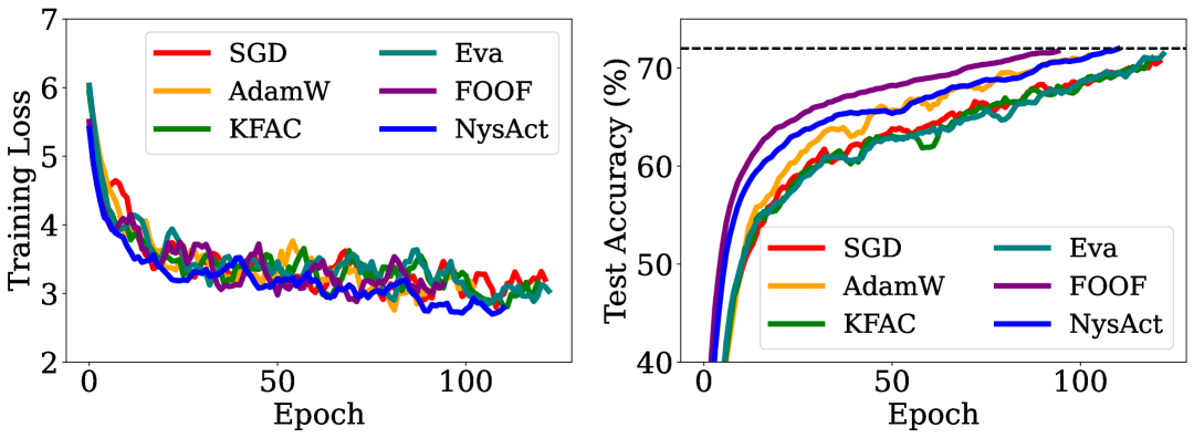
(a) ResNet-50

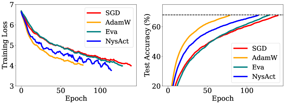
(b) DeiT-S

Figure 4: Comparison of training loss and top-1 accuracy of optimizers on ImageNet dataset. The curves are truncated at thresholds corresponding to 90% of the best top-1 accuracy achieved by SGD for each architecture.

Table 4: Top-1 accuracy (%) of ResNet-50 and DeiT-S on ImageNet dataset

Model	ResNet-50		DeiT-S
Epoch	100	200	100	200
SGD	78.05	79.46	69.08	75.27
AdamW	76.73	79.14	73.78	77.96
KFAC	78.16	79.34	69.84	✗
Eva	77.71	79.48	69.67	76.57
FOOF	78.37	79.69	65.37	✗
NysAct-S	75.62	78.77	70.72	76.16

• ✗ indicates a training failure.

Table 5: Number of epochs and wall-clock time required to achieve a threshold Top-1 accuracy for ResNet-50 (72%) and DeiT-S (68%) on ImageNet dataset

Model	ResNet-50		DeiT-S
	Epochs	Time (hrs)	Epochs	Time (hrs)
SGD	126	8.48	144	9.61
AdamW	107	7.28	83	5.59
KFAC	124	10.10	✗	✗
Eva	127	8.72	133	8.96
FOOF	99	8.33	✗	✗
NysAct-S	115	8.21	119	8.18

• ✗ indicates a training failure.

Training Results. The experimental results on ImageNet dataset are summarized in Table 4, Table 5 and Figure 4. For ResNet-50, NysAct achieves slightly lower top-1 accuracy than other baselines like SGD, AdamW, and FOOF. However, in Figure 4, we set the threshold accuracy at 72%, which corresponds to 90% of the best possible top-1 accuracy achievable by SGD in this setting. As shown, NysAct requires fewer epochs to achieve 72% top-1 accuracy compared to SGD (115 epochs vs 126), as well as second-order methods like KFAC (124 epochs) and Eva (127 epochs). While AdamW and FOOF need slightly fewer epochs to reach the threshold, NysAct still outperforms FOOF in terms of wall-clock time. It achieves the second-best time of 8.21 hours, following AdamW’s 7.28 hours, making it highly efficient compared to the 10.10 hours for KFAC and 8.72 hours for Eva. This indicates that NysAct strikes a favorable balance between computational efficiency and accuracy.

For DeiT-S, where AdamW is known for its strong performance in terms of convergence and accuracy, NysAct closely follows this benchmark. NysAct achieves the second-best top-1 accuracy at 100 epochs and performs competitively at 200 epochs, trailing AdamW and Eva. In terms of efficiency, NysAct requires 119 epochs to reach 68% top-1 accuracy (which represents 90% of the best top-1 accuracy of SGD in this architecture) compared to 144 epochs for SGD and 133 epochs for Eva. Additionally, NysAct ’s wall-clock time is shorter than that of both methods, making it the most efficient preconditioning method in this setting. On the other hand, KFAC and FOOF failed to train DeiT-S for 200 epochs due to numerical issues in preconditioner inversion. NysAct ’s strong performance with DeiT-S underscores its scalability and adaptability to attention-based architectures, even in a domain where AdamW is typically dominant.

Table 6: Comparison of relative wall-clock time and memory usage over SGD on ImageNet dataset

Model (# params)	ResNet-50 (27M)		DeiT-S (22M)
	Time	Mem	Time	Mem
KFAC	1.21$\times$	1.02$\times$	1.37$\times$	1.03$\times$
Eva	1.02$\times$	1.00$\times$	1.01$\times$	1.00$\times$
FOOF	1.25$\times$	1.01$\times$	1.11$\times$	1.02$\times$
NysAct-S	1.06$\times$	1.00$\times$	1.03$\times$	1.00$\times$

Time and Memory Complexities. Table 6 presents the efficiency of NysAct on ImageNet dataset, demonstrating its superior scalability compared to both FOOF and KFAC. Despite its faster execution, NysAct maintains memory usage on par with SGD. Additionally, NysAct achieves comparable time and memory efficiency to Eva. This highlights NysAct ’s capability to balance speed and resource efficiency across architectures, reinforcing its scalability and practicality for large-scale training.

7 Conclusion

We introduced NysAct, a scalable stochastic preconditioned gradient method that effectively reduces the computational complexity associated with activation covariance-based preconditioning while maintaining a fast convergence rate and strong generalization performance. Our extensive empirical evaluations on image classification tasks demonstrate that NysAct significantly improves end-to-end training time compared to other advanced preconditioning methods including KFAC, Eva, and FOOF. Furthermore, NysAct delivers better test accuracy compared to first-order methods such as SGD and Adam(W). By addressing the limitations of both first- and second-order methods, NysAct offers an optimal blend between them, making it a scalable yet powerful optimization choice for deep learning tasks.

Appendix A Proof of Theorem 5.5

The update rule of NysAct is given by

$${\bm{\mathrm{W}}}_{k+1}={\bm{\mathrm{W}}}_{k}-\eta{\bm{\mathrm{G}}}({\bm{\mathrm{W}}}_{k})({\bm{\mathrm{A}}}^{nys}_{k}+\rho{\bm{\mathrm{I}}})^{-1}\,,$$

where ${\bm{\mathrm{W}}}$ represents the weights in matrix form, ${\bm{\mathrm{G}}}$ is the mini-batch gradient of loss $\mathcal{L}$ w.r.t. the weights in matrix form, and ${\bm{\mathrm{A}}}^{nys}$ denotes the Nyström approximated activation covariance. The Assumption 5.4 gives the following inequalities, for all $i$:

$$\lambda_{i}({\bm{\mathrm{A}}})-\epsilon\|{\bm{\mathrm{A}}}\|_{F}\leq\lambda_{i}({\bm{\mathrm{A}}}^{nys})\leq\lambda_{i}({\bm{\mathrm{A}}})+\epsilon\|{\bm{\mathrm{A}}}\|_{F}.$$ (7)

Proof.

Using the Assumption 5.1, the Taylor expansion of the loss around ${\bm{\mathrm{W}}}_{k}$ gives

$$\mathcal{L}({\bm{\mathrm{W}}}_{k+1})\leq\mathcal{L}({\bm{\mathrm{W}}}_{k})+\langle\nabla\mathcal{L}({\bm{\mathrm{W}}}_{k}),{\bm{\mathrm{W}}}_{k+1}-{\bm{\mathrm{W}}}_{k}\rangle+\frac{L}{2}\|{\bm{\mathrm{W}}}_{k+1}-{\bm{\mathrm{W}}}_{k}\|_{F}^{2}.$$

Substituting ${\bm{\mathrm{W}}}_{k+1}-{\bm{\mathrm{W}}}_{k}=-\eta{\bm{\mathrm{G}}}({\bm{\mathrm{W}}}_{k})({\bm{\mathrm{A}}}^{nys}_{k}+\rho{\bm{\mathrm{I}}})^{-1}$, we have

$$\mathcal{L}({\bm{\mathrm{W}}}_{k+1}) \leq\mathcal{L}({\bm{\mathrm{W}}}_{k})-\eta\langle\nabla\mathcal{L}({\bm{\mathrm{W}}}_{k}),{\bm{\mathrm{G}}}({\bm{\mathrm{W}}}_{k})({\bm{\mathrm{A}}}^{nys}_{k}+\rho{\bm{\mathrm{I}}})^{-1}\rangle+\frac{\eta^{2}L}{2}\|{\bm{\mathrm{G}}}({\bm{\mathrm{W}}}_{k})({\bm{\mathrm{A}}}^{nys}_{k}+\rho{\bm{\mathrm{I}}})^{-1}\|_{F}^{2}$$

$$=\mathcal{L}({\bm{\mathrm{W}}}_{k})-\eta\operatorname{Tr}(\nabla\mathcal{L}({\bm{\mathrm{W}}}_{k})({\bm{\mathrm{A}}}^{nys}_{k}+\rho{\bm{\mathrm{I}}})^{-1}{\bm{\mathrm{G}}}({\bm{\mathrm{W}}}_{k})^{\intercal})+\frac{\eta^{2}L}{2}\|{\bm{\mathrm{G}}}({\bm{\mathrm{W}}}_{k})({\bm{\mathrm{A}}}^{nys}_{k}+\rho{\bm{\mathrm{I}}})^{-1}\|_{F}^{2}$$

$$\operatorname{Tr}({\bm{\mathrm{A}}}{\bm{\mathrm{B}}}{\bm{\mathrm{C}}})\leq\|{\bm{\mathrm{A}}}\|_{F}\|{\bm{\mathrm{B}}}{\bm{\mathrm{C}}}\|_{F}\leq\|{\bm{\mathrm{A}}}\|_{F}\|{\bm{\mathrm{B}}}\|_{2}\|{\bm{\mathrm{C}}}\|_{F} \|\cdot\|_{2}$$, where denotes the spectral norm, gives

$$\leq\mathcal{L}({\bm{\mathrm{W}}}_{k})-\eta\|\nabla\mathcal{L}({\bm{\mathrm{W}}}_{k})\|_{F}\|({\bm{\mathrm{A}}}^{nys}_{k}+\rho{\bm{\mathrm{I}}})^{-1}\|_{2}\|{\bm{\mathrm{G}}}({\bm{\mathrm{W}}}_{k})\|_{F}+\frac{\eta^{2}L}{2}\|{\bm{\mathrm{G}}}({\bm{\mathrm{W}}}_{k})\|_{F}^{2}\|({\bm{\mathrm{A}}}^{nys}_{k}+\rho{\bm{\mathrm{I}}})^{-1}\|_{F}^{2}$$

$$\leq\mathcal{L}({\bm{\mathrm{W}}}_{k})-\frac{\eta\|\nabla\mathcal{L}({\bm{\mathrm{W}}}_{k})\|_{F}\|{\bm{\mathrm{G}}}({\bm{\mathrm{W}}}_{k})\|_{F}}{\lambda_{\max}({\bm{\mathrm{A}}}^{nys}_{k})+\rho}+\frac{\eta^{2}L\|{\bm{\mathrm{G}}}({\bm{\mathrm{W}}}_{k})\|_{F}^{2}}{2(\lambda_{\min}({\bm{\mathrm{A}}}^{nys}_{k})+\rho)^{2}}$$

Assumption 5.3 and (7) yield

$$\leq\mathcal{L}({\bm{\mathrm{W}}}_{k})-\frac{\eta\|\nabla\mathcal{L}({\bm{\mathrm{W}}}_{k})\|_{F}\|{\bm{\mathrm{G}}}({\bm{\mathrm{W}}}_{k})\|_{F}}{\lambda_{\max}({\bm{\mathrm{A}}}_{k})+\epsilon\nu_{U}+\rho}+\frac{\eta^{2}L\|{\bm{\mathrm{G}}}({\bm{\mathrm{W}}}_{k})\|_{F}^{2}}{2(\lambda_{\min}({\bm{\mathrm{A}}}_{k})-\epsilon\nu_{L}+\rho)^{2}}$$

$$\leq\mathcal{L}({\bm{\mathrm{W}}}_{k})-\frac{\eta\|\nabla\mathcal{L}({\bm{\mathrm{W}}}_{k})\|_{F}\|{\bm{\mathrm{G}}}({\bm{\mathrm{W}}}_{k})\|_{F}}{\lambda_{U}+\epsilon\nu_{U}+\rho}+\frac{\eta^{2}L\|{\bm{\mathrm{G}}}({\bm{\mathrm{W}}}_{k})\|_{F}^{2}}{2(\lambda_{L}-\epsilon\nu_{L}+\rho)^{2}}.$$

Taking expectations over the training samples and using 5.2, we have

$$\operatorname{\mathbb{E}}\mathcal{L}({\bm{\mathrm{W}}}_{k+1}) \leq\operatorname{\mathbb{E}}\mathcal{L}({\bm{\mathrm{W}}}_{k})-\frac{\eta\|\nabla\mathcal{L}({\bm{\mathrm{W}}}_{k})\|_{F}^{2}}{\lambda_{U}+\epsilon\nu_{U}+\rho}+\frac{\eta^{2}L\operatorname{\mathbb{E}}\|{\bm{\mathrm{G}}}({\bm{\mathrm{W}}}_{k})\|_{F}^{2}}{2(\lambda_{L}-\epsilon\nu_{L}+\rho)^{2}}$$

$$\leq\operatorname{\mathbb{E}}\mathcal{L}({\bm{\mathrm{W}}}_{k})-\underbracket{\frac{\eta\|\nabla\mathcal{L}({\bm{\mathrm{W}}}_{k})\|_{F}^{2}}{\lambda_{U}+\epsilon\nu_{U}+\rho}}_{\leavevmode\hbox to6.41pt{\vbox to6.41pt{\text{[drawing]}}}}+\underbracket{\frac{\eta^{2}L(\sigma^{2}+\|\nabla\mathcal{L}({\bm{\mathrm{W}}}_{k})\|_{F}^{2})}{2(\lambda_{L}-\epsilon\nu_{L}+\rho)^{2}}}_{\leavevmode\hbox to6.41pt{\vbox to6.41pt{\text{[drawing]}}}}.$$ (8)

For the loss to decrease, it is necessary for the term to dominate the term . This requires that the learning rate $\eta$ be chosen as

$$\eta \leq\frac{2(\lambda_{L}-\epsilon\nu_{L}+\rho)^{2}\|\nabla\mathcal{L}({\bm{\mathrm{W}}}_{k})\|_{F}^{2}}{L(\lambda_{U}+\epsilon\nu_{U}+\rho)(\sigma^{2}+\|\nabla\mathcal{L}({\bm{\mathrm{W}}}_{k})\|_{F}^{2})}$$

$$\leq\frac{2(\lambda_{L}-\epsilon\nu_{L}+\rho)^{2}C}{L(\lambda_{U}+\epsilon\nu_{U}+\rho)(\sigma^{2}+C)}$$ (9)

Rearranging terms in (8) and summing over $T$ iterations, we have

$$\sum_{k=0}^{T-1}{\left(\frac{\eta}{\lambda_{U}+\epsilon\nu_{U}+\rho}-\frac{\eta^{2}L}{2(\lambda_{L}-\epsilon\nu_{L}+\rho)^{2}}\right)\|\nabla\mathcal{L}({\bm{\mathrm{W}}}_{k})\|_{F}^{2}} \leq\sum_{k=0}^{T-1}{\left(\operatorname{\mathbb{E}}\mathcal{L}({\bm{\mathrm{W}}}_{k})-\operatorname{\mathbb{E}}\mathcal{L}({\bm{\mathrm{W}}}_{k+1})+\frac{\eta^{2}\sigma^{2}L}{2(\lambda_{L}-\epsilon\nu_{L}+\rho)^{2}}\right)}$$

$$\leq\operatorname{\mathbb{E}}\mathcal{L}({\bm{\mathrm{W}}}_{0})-\operatorname{\mathbb{E}}\mathcal{L}({\bm{\mathrm{W}}}_{T})+\frac{\eta^{2}\sigma^{2}LT}{2(\lambda_{L}-\epsilon\nu_{L}+\rho)^{2}}$$

Assuming $$\mathcal{L}({\bm{\mathrm{W}}}_{T})\geq\mathcal{L}({\bm{\mathrm{W}}}^{*}) \mathcal{L}({\bm{\mathrm{W}}}^{*})$$, where denotes the global minima of loss function, we have

$$\leq\operatorname{\mathbb{E}}\mathcal{L}({\bm{\mathrm{W}}}_{0})-\operatorname{\mathbb{E}}\mathcal{L}({\bm{\mathrm{W}}}^{*})+\frac{\eta^{2}\sigma^{2}LT}{2(\lambda_{L}-\epsilon\nu_{L}+\rho)^{2}}$$

Dividing by $T$ and rearranging terms, we obtain the following:

$$\frac{1}{T}\sum_{k=0}^{T-1}{\|\nabla\mathcal{L}({\bm{\mathrm{W}}}_{k})\|_{F}^{2}} \leq\frac{\operatorname{\mathbb{E}}\mathcal{L}({\bm{\mathrm{W}}}_{0})-\operatorname{\mathbb{E}}\mathcal{L}({\bm{\mathrm{W}}}^{*})}{\eta T\left(\frac{1}{\lambda_{U}+\epsilon\nu_{U}+\rho}-\frac{\eta L}{2(\lambda_{L}-\epsilon\nu_{L}+\rho)^{2}}\right)}+\frac{\eta\sigma^{2}L}{2(\lambda_{L}-\epsilon\nu_{L}+\rho)^{2}-\eta L(\lambda_{U}+\epsilon\nu_{U}+\rho)}.$$

∎

Appendix B Experimental Details

Hyperparameter Settings. Table 7 outlines the hyperparameters utilized for training on CIFAR and ImageNet datasets. Here, $\eta$ refers to the learning rate, $\beta_{1}$ and $\beta_{2}$ represent the EMA coefficients for the first and second moments, and $\epsilon$ is a small constant added for numerical stability in Adam-based optimizers. In gradient preconditioning methods, $\beta_{2}$ corresponds to the EMA coefficient for preconditioner updates. The damping factor, $\rho$, controls the regularization of the covariance matrix, while $T_{cov}$ and $T_{inv}$ define the update frequencies for the covariance and inverse matrices, respectively. Lastly, $r$ denotes the approximation rank size utilized in NysAct. For CIFAR datasets, For KFAC and Eva, hyperparameter values followed the recommendations in [40]. In contrast, for FOOF and NysAct, we conducted a grid search over learning rates [$0.001,0.005,0.01,0.05,0.1,0.5$] and damping factors [$0.01,0.05,0.1,0.5,1,5,10$], while keeping the remaining settings consistent with other FIM-based preconditioners.

For ImageNet dataset, we scaled up the learning rate $\eta$ by a factor of 5 for both SGD and preconditioning methods, using a mini-batch size of $1,024$, compared to the CIFAR training, while we decrease weight decay to $0.00002$. For both ResNets and DeiT, we tripled up the damping for KFAC and Eva to mitigate instability during preconditioner inversion. For all gradient preconditioning methods, we reduced the inversion frequency from 50 to 5, enabling the models to more frequently adjust to the changes in preconditioning matrices, particularly when training DeiT.

Table 7: Hyperparameter settings for CIFAR and ImageNet datasets training

Dataset	Optimizer	$\eta$	Momentum	$\beta_{1}$	$\beta_{2}$	Weight decay	$\epsilon$	$\rho$	$T_{cov}$	$T_{inv}$	$r$
CIFAR	SGD	0.1	0.9	.	.	0.0005	.	.	.	.	.
	Adam	0.001	.	0.9	0.999	0.0005	$1\times 10^{-8}$	.	.	.	.
	AdamW	0.001	.	0.9	0.999	0.05	$1\times 10^{-8}$	.	.	.	.
	KFAC	0.1	0.9	.	0.95	0.0005	.	0.03	5	50	.
	Eva	0.1	0.9	.	0.95	0.0005	.	0.03	5	50	.
	FOOF	0.1	0.9	.	0.95	0.0005	.	1.0	5	50	.
	NysAct	0.1	0.9	.	0.95	0.0005	.	1.0	5	50	10
Dataset	Optimizer	$\eta$	Momentum	$\beta_{1}$	$\beta_{2}$	Weight decay	$\epsilon$	$\rho$	$T_{cov}$	$T_{inv}$	$r$
ImageNet	SGD	0.5	0.9	.	.	0.00002	.	.	.	.	.
	AdamW	0.001	.	0.9	0.999	0.05	$1\times 10^{-8}$	.	.	.	.
	KFAC	0.5	0.9	.	0.95	0.00002	.	0.1	5	50 / 5	.
	Eva	0.5	0.9	.	0.95	0.00002	.	0.1	5	50 / 5	.
	FOOF	0.5	0.9	.	0.95	0.00002	.	1.0	5	50 / 5	.
	NysAct	0.5	0.9	.	0.95	0.00002 / 0.0001	.	1.0	5	50 / 5	50 / 20

Model Settings for ResNets and DeiT. Table 8 summarizes the configurations used for training on the ImageNet dataset. Two architectures were explored: ResNet and DeiT-Small. For ResNet, we followed the PyTorch implementation [27], and for DeiT, we applied the settings from [33]. Both models incorporated advanced training techniques such as Random Erasing [41], Label Smoothing [31], Mixup/CutMix [39, 38], and Repeated Augmentation [15]. ResNet used TrivialAugment [26], while DeiT employed RandAugment [4] and Stochastic Depth [18]. Training was conducted at a resolution of 176 for ResNet and 224 for DeiT, with both models evaluated at a test resolution of 224. A mini-batch size of 1,024 was used with cosine learning rate decay and a 5-epoch warmup.

Table 8: Settings for ImageNet training

Architecture	ResNets	DeiT
Train Res	176	224
Test Res	224	224
Batch size	1,024	1,024
LR decay	cosine	cosine
Warmup epochs	5	5
Label Smoothing	0.1	0.1
Stochastic Depth	-	0.2
Repeated Augmentation	✓	✓
Horizontal flip	✓	✓
Random Resized Crop	✓	✓
Auto Augmentation	TrivialAugment	RandAugment(9/0.5)
Mixup	0.2	0.8
Cutmix	1.0	1.0
Random Erasing	0.1	0.25

Appendix C Hyperparameter Study

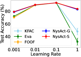
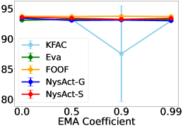
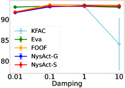
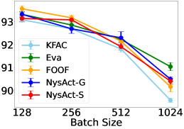
Figure 5: Comparison of the effects of learning rate, EMA coefficient, damping, and mini-batch size on gradient preconditioning methods, training ResNet-32 on CIFAR-10 for 100 epochs

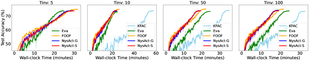
Figure 6: Comparison of wall-clock time for different inverse update frequencies during ResNet-110 training on the CIFAR-100 dataset

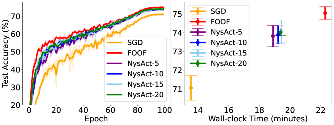
(a) NysAct-Gaussian Sampling

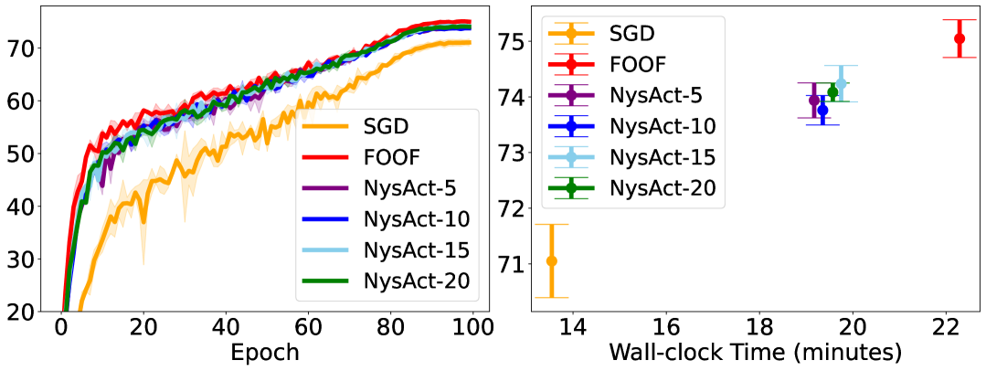
(b) NysAct-Uniform Column Sampling

Figure 7: Comparison of test accuracy and wall-clock time for different ranks of NysAct during ResNet-110 training on CIFAR-100 dataset. The errorbar plots illustrate the comparison of test accuracy and wall-clock time for each method at their optimal epoch during the 100-epoch training period, along with the corresponding computational time in minutes.

We performed an ablation study on NysAct and compared its results with other gradient preconditioning methods. We chose KFAC, Eva, and FOOF as baselines because they all rely on approximations of FIM and share similar hyperparameters, making them ideal for direct comparison with NysAct. This analysis was carried out using ResNet-32 on CIFAR-10 and ResNet-110 on CIFAR-100, each trained for 100 epochs across three different runs.

Essential Hyperparameters. Figure 5 provides a comprehensive comparison of NysAct with KFAC, Eva, and FOOF, focusing on essential hyperparameter tuning. The first subplot highlights that all methods, including NysAct, perform best at a learning rate of 0.1. At the lower end of learning rate, i.e., when learning rate $\leq 0.01$, Eva and FOOF struggle and show a drop in performance. On the higher end, at the learning rate of 1.0, KFAC and Eva experience significant performance degradation. In contrast, NysAct maintains stable and consistent performance across the entire range of learning rates tested. In the second subplot, NysAct, along with the other methods, demonstrates consistent performance across different EMA coefficients, with the exception of KFAC. This suggests that NysAct’s performance remains largely unaffected by changes of the EMA coefficient, whereas KFAC exhibits noticeable fluctuations, particularly at a coefficient value of 0.9. In the third subplot, NysAct’s test accuracy increases as the damping factor $\rho$ increases from 0.1 to 10.0. At a damping value of 0.01, both FOOF and NysAct experience a slight dip in performance relative to KFAC and Eva. However, when the damping value reaches 10.0, KFAC displays significant variability and a marked decline in performance. The observation in the last subplot aligns with the broader trend in optimization, where large-batch training often leads to degraded network performance, as highlighted in previous research [12, 16]. Among the methods compared, NysAct experiences a moderate decrease in test accuracy as the batch size grows, showing a more stable performance relative to other baselines.

Inverse Update Frequencies. Figure 6 shows the effects of varying inverse update frequencies for the preconditioning matrix, testing intervals of 5, 10, 50, and 100 steps. The results suggest that increasing the update frequency does not significantly compromise the test accuracy of NysAct, while it contributes to reducing computational overhead. For update frequencies of 10 steps or more, NysAct achieved the fastest training time while maintaining the second-best test accuracy, just behind FOOF. At a frequency of 5 steps, Eva exhibited the fastest overall training time, with FOOF being the slowest. NysAct demonstrated a slightly faster training time than FOOF. KFAC is absent from this subplot due to its frequent failures in inverting the preconditioners. Notably, when $\tau_{inv}=50$ and $\tau_{inv}=100$ steps, Eva, despite being the lightest and most scalable variant of KFAC, became slower than FOOF in this settings.

Impact of Rank on NysAct. Figure 7 presents the impact of the rank hyperparameter in NysAct. The subplots on the left display the results for NysAct-G, while those on the right show the results for NysAct-S. In both cases, NysAct outperforms SGD in test accuracy and closely follows FOOF. When comparing the sketching methods, Gaussian sampling exhibits larger variability in test accuracy compared to subcolumn sampling, though both methods achieve similar performance, around 74% test accuracy. As the rank increases, there is a subtle trend of improved test accuracy for both sampling methods, aligning with the expectation that higher-rank approximations better capture the original matrix’s properties. The findings suggest that NysAct effectively approximates the exact activation covariance matrix with low ranks, as evidenced by the minimal difference in test accuracy between rank-5 and rank-20 approximations, with overlapping error bars indicating negligible variance.

References

- [1] Naman Agarwal, Brian Bullins, Xinyi Chen, Elad Hazan, Karan Singh, Cyril Zhang, and Yi Zhang. Efficient full-matrix adaptive regularization. In International Conference on Machine Learning, 2020.
- [2] Frederik Benzing. Gradient descent on neurons and its link to approximate second-order optimization. In International Conference on Machine Learning, 2022.
- [3] C. G. Broyden. The convergence of a class of double-rank minimization algorithms 2. the new algorithm. Ima Journal of Applied Mathematics, 1970.
- [4] Ekin Dogus Cubuk, Barret Zoph, Jonathon Shlens, and Quoc V. Le. Randaugment: Practical automated data augmentation with a reduced search space. IEEE/CVF Conference on Computer Vision and Pattern Recognition Workshops, 2019.
- [5] Jia Deng, Wei Dong, Richard Socher, Li-Jia Li, Kai Li, and Li Fei-Fei. Imagenet: A large-scale hierarchical image database. In IEEE conference on computer vision and pattern recognition, 2009.
- [6] R. Fletcher. A new approach to variable metric algorithms. Comput. J., 1970.
- [7] Zachary Frangella, Pratik Rathore, Shipu Zhao, and Madeleine Udell. Sketchysgd: reliable stochastic optimization via randomized curvature estimates. arXiv, 2022.
- [8] Zachary Frangella, Joel A. Tropp, and Madeleine Udell. Randomized nyström preconditioning. SIAM J. Matrix Anal. Appl., 2023.
- [9] Elias Frantar, Eldar Kurtic, and Dan Alistarh. M-FAC: Efficient matrix-free approximations of second-order information. In A. Beygelzimer, Y. Dauphin, P. Liang, and J. Wortman Vaughan, editors, Neural Information Processing Systems, 2021.
- [10] Donald Goldfarb. A family of variable-metric methods derived by variational means. Mathematics of Computation, 1970.
- [11] Donald Goldfarb, Yi Ren, and Achraf Bahamou. Practical quasi-newton methods for training deep neural networks. In Neural Information Processing Systems, 2020.
- [12] Priya Goyal, Piotr Dollár, Ross B. Girshick, Pieter Noordhuis, Lukasz Wesolowski, Aapo Kyrola, Andrew Tulloch, Yangqing Jia, and Kaiming He. Accurate, large minibatch sgd: Training imagenet in 1 hour. ArXiv, 2017.
- [13] Vineet Gupta, Tomer Koren, and Yoram Singer. Shampoo: Preconditioned stochastic tensor optimization. In International Conference on Machine Learning, 2018.
- [14] Kaiming He, Xiangyu Zhang, Shaoqing Ren, and Jian Sun. Deep residual learning for image recognition. In IEEE Conference on Computer Vision and Pattern Recognition, 2016.
- [15] Elad Hoffer, Tal Ben-Nun, Itay Hubara, Niv Giladi, Torsten Hoefler, and Daniel Soudry. Augment your batch: better training with larger batches. ArXiv, 2019.
- [16] Elad Hoffer, Itay Hubara, and Daniel Soudry. Train longer, generalize better: closing the generalization gap in large batch training of neural networks. In Neural Information Processing Systems, 2017.
- [17] Gao Huang, Zhuang Liu, and Kilian Q. Weinberger. Densely connected convolutional networks. IEEE Conference on Computer Vision and Pattern Recognition (CVPR), 2016.
- [18] Gao Huang, Yu Sun, Zhuang Liu, Daniel Sedra, and Kilian Q. Weinberger. Deep networks with stochastic depth. In European Conference on Computer Vision, 2016.
- [19] Diederik P. Kingma and Jimmy Ba. Adam: A method for stochastic optimization. In International Conference on Learning Representations, 2015.
- [20] Alex Krizhevsky. Learning multiple layers of features from tiny images. Technical report, Citeseer, 2009.
- [21] Y. Lecun, L. Bottou, Y. Bengio, and P. Haffner. Gradient-based learning applied to document recognition. Proceedings of the IEEE, 1998.
- [22] Hong Liu, Zhiyuan Li, David Leo Wright Hall, Percy Liang, and Tengyu Ma. Sophia: A scalable stochastic second-order optimizer for language model pre-training. In International Conference on Learning Representations, 2024.
- [23] Ilya Loshchilov and Frank Hutter. Sgdr: Stochastic gradient descent with warm restarts. International Conference on Learning Representations, 2016.
- [24] Ilya Loshchilov and Frank Hutter. Decoupled weight decay regularization. In International Conference on Learning Representations, 2019.
- [25] James Martens and Roger Grosse. Optimizing neural networks with kronecker-factored approximate curvature. In International Conference on Machine Learning, 2015.
- [26] Samuel G. Müller and Frank Hutter. Trivialaugment: Tuning-free yet state-of-the-art data augmentation. IEEE/CVF International Conference on Computer Vision, 2021.
- [27] Adam Paszke, Sam Gross, Francisco Massa, Adam Lerer, James Bradbury, Gregory Chanan, Trevor Killeen, Zeming Lin, Natalia Gimelshein, Luca Antiga, Alban Desmaison, Andreas Kopf, Edward Yang, Zachary DeVito, Martin Raison, Alykhan Tejani, Sasank Chilamkurthy, Benoit Steiner, Lu Fang, Junjie Bai, and Soumith Chintala. Pytorch: An imperative style, high-performance deep learning library. In Neural Information Processing Systems, 2019.
- [28] Archan Ray, Nicholas Monath, Andrew McCallum, and Cameron Musco. Sublinear time approximation of text similarity matrices. In AAAI Conference on Artificial Intelligence, 2021.
- [29] Herbert Robbins and Sutton Monro. A stochastic approximation method. The annals of mathematical statistics, 1951.
- [30] David F. Shanno. Conditioning of quasi-newton methods for function minimization. Mathematics of Computation, 1970.
- [31] Christian Szegedy, Vincent Vanhoucke, Sergey Ioffe, Jonathon Shlens, and Zbigniew Wojna. Rethinking the inception architecture for computer vision. IEEE Conference on Computer Vision and Pattern Recognition, 2015.
- [32] Zedong Tang, Fenlong Jiang, Maoguo Gong, Hao Li, Yue Wu, Fan Yu, Zidong Wang, and Min Wang. Skfac: Training neural networks with faster kronecker-factored approximate curvature. IEEE/CVF Conference on Computer Vision and Pattern Recognition, 2021.
- [33] Hugo Touvron, Matthieu Cord, Matthijs Douze, Francisco Massa, Alexandre Sablayrolles, and Herv’e J’egou. Training data-efficient image transformers & distillation through attention. In International Conference on Machine Learning, 2020.
- [34] Hoang Tran and Ashok Cutkosky. Better SGD using second-order momentum. In Neural Information Processing Systems, 2022.
- [35] Joel A. Tropp, Alp Yurtsever, Madeleine Udell, and Volkan Cevher. Fixed-rank approximation of a positive-semidefinite matrix from streaming data. In Neural Information Processing Systems, 2017.
- [36] Christopher K. I. Williams and Matthias W. Seeger. Using the nyström method to speed up kernel machines. In Neural Information Processing Systems, 2000.
- [37] Zhewei Yao, Amir Gholami, Sheng Shen, Kurt Keutzer, and Michael W. Mahoney. Adahessian: An adaptive second order optimizer for machine learning. In AAAI Conference on Artificial Intelligence, 2020.
- [38] Sangdoo Yun, Dongyoon Han, Seong Joon Oh, Sanghyuk Chun, Junsuk Choe, and Young Joon Yoo. Cutmix: Regularization strategy to train strong classifiers with localizable features. IEEE/CVF International Conference on Computer Vision, 2019.
- [39] Hongyi Zhang, Moustapha Cisse, Yann N. Dauphin, and David Lopez-Paz. mixup: Beyond empirical risk minimization. In International Conference on Learning Representations, 2018.
- [40] Lin Zhang, Shaohuai Shi, and Bo Li. Eva: Practical second-order optimization with kronecker-vectorized approximation. In International Conference on Learning Representations, 2023.
- [41] Zhun Zhong, Liang Zheng, Guoliang Kang, Shaozi Li, and Yi Yang. Random erasing data augmentation. AAAI Conference on Artificial Intelligence, 2017.