An Adaptive Method Stabilizing Activations for Enhanced Generalization

Abstract

We introduce AdaAct, a novel optimization algorithm that adjusts learning rates according to activation variance. Our method enhances the stability of neuron outputs by incorporating neuron-wise adaptivity during the training process, which subsequently leads to better generalization—a complementary approach to conventional activation regularization methods. Experimental results demonstrate AdaAct’s competitive performance across standard image classification benchmarks. We evaluate AdaAct on CIFAR and ImageNet, comparing it with other state-of-the-art methods. Importantly, AdaAct effectively bridges the gap between the convergence speed of Adam and the strong generalization capabilities of SGD, all while maintaining competitive execution times. Code is available at https://github.com/hseung88/adaact

Keywords Deep learning optimization  $\cdot$ Adaptive gradient methods  $\cdot$ Gradient preconditioning

This is the extended version of the paper published in the 2024 IEEE International Conference on Data Mining Workshops (ICDMW), © IEEE. The published version is available at: 10.1109/ICDMW65004.2024.00007

1 Introduction

Adaptive gradient methods such as Adam kingma2015adam and its variants liu2020Adam have been the method of choice for training deep neural networks (NNs) due to their faster convergence compared to SGD Sutskever2013OnTI . However, a line of studies Wilson2017TheMV ; Chen2018ClosingTG ; Reddi2019OnTC has reported the cases in which these adaptive methods diverge or result in worse generalization performance than SGD. While several optimizers such as SWAT keskar2017improving , AdaBound Luo2019AdaBound , and Padam chen2020closing have been proposed to mitigate the issue, these methods mostly focus on establishing optimization bounds on the training objective, ignoring the generalization and stability properties of the model being trained.

Recent work has investigated the connection between activation stability and generalization properties of neural networks and empirically demonstrated that stabilizing the output can help improve the generalization performance. These works proposed approaches to maintain stable output distribution among layers, which includes explicitly normalizing the activations srivastava14dropout ; ioffe15batch ; Ba2016LayerN , adding a loss term to penalize the activation variance krueger2015regularizing ; Littwin2018RegularizingBT ; Ding2019RegularizingAD , or regularizing the output into the standard normal distribution Joo2020RegularizingAI . Orthogonal to prior approaches that rely on activation regularization, in this work, we devise an optimization method, called AdaAct, that directly promotes stable neuron outputs during training. Specifically, to stabilize the activations during training, AdaAct carefully controls the magnitude of updates according to the estimated activation variance. This is in contrast to vast majority of other adaptive gradient methods that adapt to gradient variance. Our strategy involves taking smaller steps when encountering high activation variance and, conversely, taking larger steps in the presence of low activation variance. This is achieved by maintaining the running mean of activation variance and scaling the gradient update inversely proportional to the square root of the variance. Seemingly our method may look similar to FOOF Benzing2022GradientDO or LocoProp Amid2021LocoPropEB as these methods use activation covariance matrix to precondition the gradient. However, we emphasize that our method is developed with a completely different motivation of activation stabilization via variance adaptation, while their analyses primarily focus on investigating the effectiveness of Kronecker-Factored approximation in KFAC martens2015optimizing and the connection between their optimizer and second-order methods. In addition, these methods are inefficient as they require storing a large covariance matrix for each layer and involve costly matrix inversion operation. In contrast, our method assumes the independence between activations and only computes the variance of individual activations (which corresponds to the diagonal entries in the covariance matrix). Our method is also different from other adaptive gradient methods that maintain a per-parameter learning rate in the sense that it applies a less aggressive adaptation strategy to avoid the pitfall of too much adaptation. In our method, the parameters that interact with the same input share the same learning rate.

To demonstrate the effect of adapting gradient to activation variance, we train LeNet-5 lecun98lenet5 on CIFAR10 krizhevsky2009learning dataset using our proposed method and visualize the activation variance (averaged over entire training iterations) and test accuracy in Figure 1. To calculate the averaged activation variance, we first flatten the activations of these layers and compute the variance for each activation. Then we average these variances over iterations. As shown in the figure, the network trained using AdaAct yields the smallest activation variance in all layers and achieves higher test accuracy at the end of training compared to momentum SGD and Adam. Adam shows faster convergence at the early stage of training thanks to its fast adaptation capability, which results in higher activation variance. See Figure 8 in Appendix D for the unaveraged activation variance plots.

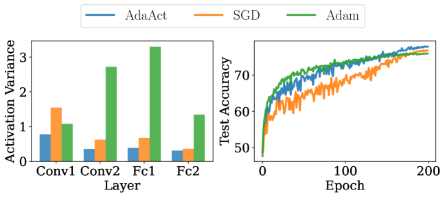
Figure 1: (Left) Averaged activation variance from each hidden layer and (Right) test accuracy training LeNet-5 on CIFAR10.

The key contributions of our work can be summarized as follows:

• We propose a novel optimizer that stabilizes the neuron outputs via activation variance adaptation.

• Our proposed method demonstrates improved generalization compared to state-of-the-art adaptive methods. Its convergence speed is similar to that of Adam while at the end of training it achieves good generalization performance comparable to that of highly tuned SGD.

• To evaluate the performance of proposed method, we conduct extensive experiments on image classification task with CIFAR 10/100 and ImageNet dataset using various architectures, including ResNet, DenseNet, and ViT. Importantly, it achieves enhanced performance while maintaining a comparable execution time to other adaptive methods.

2 Related Work

In this section, we provide an overview of relevant literature that both underpins and complements our work.

Adaptive Methods.

Adaptive methods such as AdaGrad duchi2011adaptive , RMSProp hinton12rmsprop , and Adam kingma2015adam have enhanced NN training due to their superior convergence speeds compared to SGD Sutskever2013OnTI . However, concerns have emerged about over-specialization with these methods, potentially impacting model generalization. Specifically, Wilson2017TheMV pointed out that these methods might accentuate the generalization gap compared to SGD. Additionally, Chen2018ClosingTG highlighted high adaptivity as a root cause, and Reddi2019OnTC mentioned contexts where Adam may not converge. In response to these challenges, a variety of optimization methods have been proposed. Nadam dozat2016incorporating synergizes the advantages of Adam and Nesterov’s accelerated gradient to promote better convergence and generalization. Padam Chen2018ClosingTG features a tunable hyperparameter to bridge the gap between Adam and SGD. AdamW Loshchilov2019DecoupledWD decouples weight decay from adaptive learning rates. AdaBound Luo2019AdaBound modulates the learning rates in adaptive methods, bounding them based on the traditional SGD approach. AMSGrad Reddi2019OnTC enforces bounds on learning rates by leveraging the maximum observed moving average value. AdaBelief zhuang2020adabelief monitors the moving average of squared gradient discrepancies versus their respective moving average, differentiating genuine gradient noise from actual gradient shifts. Adai Xie2020AdaptiveID isolates the influences of the adaptive learning rate and momentum within Adam dynamics. Lastly, Radam Liu2020OnTV incorporates a term that tempers the adaptivity of learning rates in initial training phases, fostering more consistent and dependable training.

Activation Regularization.

Recent studies have emphasized the significance of regularizing activations for better model generalization. Dropout srivastava14dropout randomly nullifies activations, preventing overreliance. Batch normalization ioffe15batch and layer normalization Ba2016LayerN maintain consistent activation distributions across batches or features respectively. krueger2015regularizing proposed a regularization technique for recurrent neural networks (RNNs) that mitigates abrupt activation changes, while Merity2017RevisitingAR delved deeper into activation regularization for language tasks with RNNs. Littwin2018RegularizingBT and Joo2020RegularizingAI targeted consistent activations across batches; the former used the variance of their sample-variances, while the latter employed the Wasserstein distance. Ding2019RegularizingAD suggested distribution loss for binarized networks, and Fu2022NeuronWS argued consistent neuronal responses enhance generalization in NNs.

Covariance-based Gradient Preconditioning.

Ida2016AdaptiveLR introduced an adaptive method that preconditions gradient descent using the gradient covariance matrix, different from our approach of using the activation covariance matrix as a preconditioner. FOOF Benzing2022GradientDO explicitly utilizes activation covariance for gradient preconditioning. In parallel, LocoProp Amid2021LocoPropEB introduced a framework of layerwise loss construction, and their update equation aligns with FOOF’s when employing a local squared loss. Eva Zhang2023EvaPS proposed a second-order algorithm that utilizes a variant of the two covariance matrices from KFAC, leveraging the Sherman-Morrison formula.

3 Preliminaries

We consider solving the following optimization problem:

$$\min_{\bm{\mathrm{\theta}}\in\mathbb{R}^{d}}F(\bm{\mathrm{\theta}}):=\operatorname{\mathbb{E}}_{\xi\sim\mathcal{D}}\left[f(\bm{\mathrm{\theta}};\xi)\right]\,,$$ (1)

where $f:\mathbb{R}^{d}\to\mathbb{R}$ is differentiable and possibly nonconvex in $\bm{\mathrm{\theta}}$ and $\xi$ is a random variable following an unknown but fixed distribution $\mathcal{D}$. In the context of machine learning, $F$ corresponds to the empirical risk, i.e., $F(\bm{\mathrm{\theta}})=\mathcal{L}(\bm{\mathrm{\theta}};S):=\frac{1}{N}\sum_{i=1}^{N}\ell(\bm{\mathrm{\theta}};\bm{\mathrm{x}}_{i},y_{i})$, where $\ell$ is a loss function, $S=\{(\bm{\mathrm{x}}_{i},y_{i})\}_{i=1}^{N}$ is the training dataset, and $\bm{\mathrm{\theta}}$ corresponds to model parameters.

3.1 Notations

For vectors, we use element-wise operations unless specified otherwise. $(\bm{\mathrm{x}})_{i}$ denotes the $i$-th coordinate of $\bm{\mathrm{x}}$. $\lVert\bm{\mathrm{x}}\rVert$ represents $L_{2}$ norm unless stated otherwise. We use $[N]$ to denote the set $\{1,2,\dots,N\}$, $\otimes$ to represent the Kronecker product, and $\odot$ for the Hadamard product. Consider a feed-forward NN consisting of $L$ layers trained on a dataset $S=\{(\bm{\mathrm{x}}_{i},y_{i})\}_{i=1}^{n}$. Let ${\bm{\mathrm{W}}}$ and $\bm{\mathrm{b}}$ be the weight and bias of layer $\ell\in[L]$. It is often convenient to include the bias term into the weight ${\bm{\mathrm{W}}}$ as the last column: ${\bm{\mathrm{\Theta}}}^{(\ell)}=\begin{bmatrix}{\bm{\mathrm{W}}}^{(\ell)}&\bm{\mathrm{b}}^{(\ell)}\end{bmatrix}\in\mathbb{R}^{m_{\ell}\times(m_{\ell-1}+1)}\,$. We augment each $\bm{\mathrm{a}}^{(\ell)}\in\mathbb{R}^{m_{\ell}}$ by adding a $1$ to its last entry and denote it by $\tilde{\bm{\mathrm{a}}}^{(\ell)}\in\mathbb{R}^{m_{\ell}+1}$. The forward step of our NN is given by

$$\bm{\mathrm{z}}^{(\ell)} ={\bm{\mathrm{\Theta}}}^{(\ell)}\tilde{\bm{\mathrm{a}}}^{(\ell-1)}\in\mathbb{R}^{m_{\ell}}\,,\qquad\bm{\mathrm{a}}^{(\ell)}=\phi(\bm{\mathrm{z}}^{(\ell)})\in\mathbb{R}^{m_{\ell}}\,,$$

$$\bm{\mathrm{\theta}}^{(\ell)} =\operatorname{vec}({\bm{\mathrm{\Theta}}}^{(\ell)})\in\mathbb{R}^{m_{\ell}(m_{\ell-1}+1)}\,,$$

where $\bm{\mathrm{z}}$, $\bm{\mathrm{a}}$, and $\phi$ represent the pre-activations, activations, and an activation function, respectively, and $\tilde{\bm{\mathrm{a}}}^{(0)}=\bm{\mathrm{x}}$. The vectorization operator, denoted by $\operatorname{vec}(\cdot)$, takes ${\bm{\mathrm{X}}}\in\mathbb{R}^{m\times n}$ as input and returns a vector $\operatorname{vec}({\bm{\mathrm{X}}})\in\mathbb{R}^{mn}$ of length $mn$. That is, $\operatorname{vec}({\bm{\mathrm{X}}})=\begin{bmatrix}{\bm{\mathrm{X}}}_{*,1}^{\intercal}&{\bm{\mathrm{X}}}_{*,2}^{\intercal}&\cdots&{\bm{\mathrm{X}}}_{*,n}^{\intercal}\end{bmatrix}^{\intercal}\,$, where ${\bm{\mathrm{X}}}_{*,j}$ denotes the $j$^th column of matrix ${\bm{\mathrm{X}}}$.

3.2 Kronecker Factored Approximate Curvature

martens2015optimizing introduced KFAC which approximates the Fisher information matrix (FIM) as $(\widetilde{{\bm{\mathrm{F}}}})_{i,j}={\bm{\mathrm{A}}}_{i-1,j-1}\otimes{\bm{\mathrm{P}}}_{i,j}$, where ${\bm{\mathrm{A}}}_{i,j}=\operatorname{\mathbb{E}}\left[\tilde{\bm{\mathrm{a}}}^{(i)}(\tilde{\bm{\mathrm{a}}}^{(j)})^{\intercal}\right]$ denotes the covariance of the activations from layer $i$ and $j$, and ${\bm{\mathrm{P}}}_{i,j}=\operatorname{\mathbb{E}}\left[\frac{\partial\mathcal{L}}{\partial\bm{\mathrm{z}}^{(i)}}\frac{\partial\mathcal{L}}{\partial\bm{\mathrm{z}}^{(j)}}^{\intercal}\right]$ represents the covariance of pre-activation gradients between layer $i$ and $j$. Assuming the independence between layer $i$ and $j$ for $i\neq j$, KFAC only computes the diagonal blocks of FIM, denoted by ${\bm{\mathrm{A}}}^{(\ell-1)}\otimes{\bm{\mathrm{P}}}^{(\ell)}={\bm{\mathrm{A}}}_{\ell-1,\ell-1}\otimes{\bm{\mathrm{P}}}_{\ell,\ell}$ , which results in the following update rule for layer $\ell$ at iteration $t$.

$$\bm{\mathrm{\theta}}_{t+1}^{(\ell)} =\bm{\mathrm{\theta}}_{t}^{(\ell)}-\eta({\bm{\mathrm{A}}}_{t}^{(\ell-1)}\otimes{\bm{\mathrm{P}}}_{t}^{(\ell)})^{-1}\operatorname{vec}(\nabla_{{\bm{\mathrm{\Theta}}}^{(\ell)}}{\mathcal{L}_{t}})$$

$$=\bm{\mathrm{\theta}}_{t}^{(\ell)}-\eta\operatorname{vec}{\big{(}({\bm{\mathrm{P}}}_{t}^{(\ell)})^{-1}\nabla_{{\bm{\mathrm{\Theta}}}^{(\ell)}}{\mathcal{L}_{t}}({\bm{\mathrm{A}}}_{t}^{(\ell-1)})^{-1}\big{)}},$$ (2)

where $\eta$ is learning rate and $\nabla_{{\bm{\mathrm{\Theta}}}^{(\ell)}}{\mathcal{L}_{t}}\in\mathbb{R}^{m_{\ell}\times(m_{\ell-1}+1)}$ is the gradient of $\mathcal{L}$ w.r.t. the parameters of layer $\ell$ evaluated at time $t$. Benzing2022GradientDO argued that the pre-activation gradient term ${\bm{\mathrm{P}}}$, in fact, does not contribute to superior performance of KFAC and proposed the following update:

$$\bm{\mathrm{\theta}}_{t+1}^{(\ell)}=\bm{\mathrm{\theta}}_{t}^{(\ell)}-\eta\operatorname{vec}{\big{(}\nabla_{{\bm{\mathrm{\Theta}}}_{t}}{\mathcal{L}}({\bm{\mathrm{A}}}_{t}^{(\ell-1)})^{-1}\big{)}}\,.$$ (3)

The above equation is derived by applying the principle that an update of the weight matrix explicitly changes the layer’s outputs (pre-activations) into their gradient direction (pre-activation gradients). Mathematically, this can be expressed as $({\bm{\mathrm{{\bm{\mathrm{\Theta}}}}}}+\Delta{\bm{\mathrm{{\bm{\mathrm{\Theta}}}}}})\tilde{\bm{\mathrm{a}}}=\bm{\mathrm{z}}+\eta\frac{\partial\mathcal{L}}{\partial\bm{\mathrm{z}}}$ and such $\Delta{\bm{\mathrm{{\bm{\mathrm{\Theta}}}}}}$ is obtained by solving $\min_{\Delta{\bm{\mathrm{{\bm{\mathrm{\Theta}}}}}}}{||\left(\Delta{\bm{\mathrm{{\bm{\mathrm{\Theta}}}}}}\right)\tilde{\bm{\mathrm{a}}}-\eta\frac{\partial\mathcal{L}}{\partial\bm{\mathrm{z}}}||^{2}}+\frac{\lambda}{2}||\Delta{\bm{\mathrm{{\bm{\mathrm{\Theta}}}}}}||^{2}$. This suggests that obtaining optimized neuron outputs in NNs is closely connected to preconditioning gradients with activation covariance, which motivated the activation variance-based adaptation in AdaAct.

4 Algorithm

In this section, we introduce AdaAct, for solving the optimization problem (1). The pseudocode of algorithm is presented in Algorithm 1.

For layer $\ell$, the input activation covariance matrix ${\bm{\mathrm{A}}}_{t}^{(\ell-1)}$ can be estimated using the samples in minibatch $\mathcal{B}_{t}$.

$${\bm{\mathrm{A}}}_{t}^{(\ell-1)} =\operatorname{\mathbb{E}}\left[\tilde{\bm{\mathrm{a}}}^{(\ell-1)}(\tilde{\bm{\mathrm{a}}}^{(\ell-1)})^{\intercal}\right]\in\mathbb{R}^{(m_{\ell-1}+1)\times(m_{\ell-1}+1)}$$

$$\approx\frac{1}{\lvert\mathcal{B}_{t}\rvert}\sum_{i\in\mathcal{B}_{t}}\tilde{\bm{\mathrm{a}}}^{(\ell-1)}_{i}(\tilde{\bm{\mathrm{a}}}^{(\ell-1)}_{i})^{\intercal}\,,$$ (4)

where $\bm{\mathrm{a}}^{(\ell-1)}_{i}$ denotes the activation of layer $\ell-1$ when the input to the network is the $i$^th example $\bm{\mathrm{x}}_{i}$ in the training set. The covariance matrix in (4) could be large for many modern large scale neural networks (e.g., ViT). For a network with $L$ layers, it requires storing $\sum_{\ell=0}^{L-1}m_{\ell}^{2}$ entries. Even worse, computing its inverse takes $\mathcal{O}(m_{\ell}^{3})$ time in general.

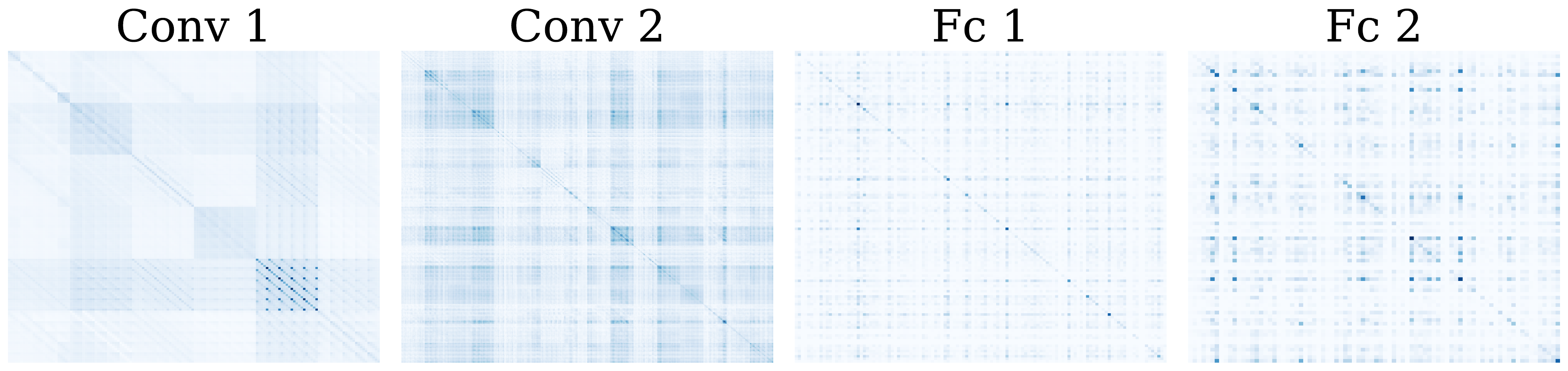
Figure 2: Heatmap of the activation covariance from the hidden layers of LeNet-5 trained on CIFAR10.

Figure 2 presents heatmaps of the activation covariance of each hidden layer. Due to the use of ReLU activation function in many modern neural networks, the activation covariance matrix is sparse, and the entries in diagonal positions tend to have relatively larger magnitude than other entries. From these observations, AdaAct approximates ${\bm{\mathrm{A}}}_{t}^{(\ell-1)}$ as a diagonal matrix — this results in lower space complexity than Adam – and applies the weighted averaging. Line 5 computes the exponential moving average (EMA) of the second moment of activations where both ${\bm{\mathrm{V}}}_{t}$ and $\widetilde{{\bm{\mathrm{A}}}}_{t}$ belong to $\mathbb{R}^{(m_{\ell-1}+1)\times(m_{\ell-1}+1)}$. While the algorithm appears to resemble Adam, it was derived from a different perspective. Specifically, in Line 5 of Algorithm 1, AdaAct replaces the EMA of squared gradient in Adam with that of activation variance. Our algorithm can be viewed as dynamically adjusting the learning rates according to the variance of activations.

Algorithm 1 AdaAct

Require: Learning rate $\eta_{t}$, Momentum $\beta_{1}=0.9,\ \beta_{2}=0.999$, Weight decay $\lambda$, Numerical stability $\epsilon$
Initialize: $\bm{\mathrm{\theta}}_{0}$, ${\bm{\mathrm{M}}}_{0}={\bm{\mathrm{O}}}$, ${\bm{\mathrm{V}}}_{0}={\bm{\mathrm{O}}}$
Output: $\bm{\mathrm{\theta}}_{t}\in\mathbb{R}^{m_{\ell}(m_{\ell-1}+1)}$

1: for $t$=1,2,3, … do

2:  Draw a mini-batch $\mathcal{B}_{t}$ of samples.

3:  $\circ$ EMA of activation variance:

4:  $\widetilde{{\bm{\mathrm{A}}}}_{t}=\frac{1}{|\mathcal{B}_{t}|}\sum_{i\in\mathcal{B}_{t}}{\operatorname{diag}(\tilde{\bm{\mathrm{a}}}_{i}\tilde{\bm{\mathrm{a}}}_{i}^{\intercal})}\in\mathbb{R}^{(m_{\ell-1}+1)\times(m_{\ell-1}+1)}$

5:  ${\bm{\mathrm{V}}}_{t}=\beta_{2}{\bm{\mathrm{V}}}_{t-1}+(1-\beta_{2})\widetilde{{\bm{\mathrm{A}}}}_{t}$

6:  $\widehat{{\bm{\mathrm{V}}}}_{t}={\bm{\mathrm{V}}}_{t}\ /\ (1-\beta_{2}^{t})$

7:  $\circ$ EMA of gradient:

8:  ${\bm{\mathrm{G}}}_{t}=\frac{1}{|\mathcal{B}_{t}|}\sum_{i\in\mathcal{B}_{t}}\nabla{\ell}(\bm{\mathrm{\Theta}}_{t};\bm{\mathrm{x}}_{i})\in\mathbb{R}^{m_{\ell}\times(m_{\ell-1}+1)}$

9:  ${\bm{\mathrm{M}}}_{t}=\beta_{1}{\bm{\mathrm{M}}}_{t-1}+(1-\beta_{1}){\bm{\mathrm{G}}}_{t}$

10:  $\widehat{{\bm{\mathrm{M}}}}_{t}={\bm{\mathrm{M}}}_{t}\ /\ (1-\beta_{1}^{t})$

11:  $\circ$ Variance adaptation:

12:  $\widehat{{\bm{\mathrm{G}}}}_{t}=\widehat{{\bm{\mathrm{M}}}}_{t}\left(\sqrt{\widehat{{\bm{\mathrm{V}}}}_{t}}+\epsilon{\bm{\mathrm{I}}}\right)^{-1}$

13:  $\widehat{\bm{\mathrm{g}}}_{t}=\operatorname{vec}{(\widehat{{\bm{\mathrm{G}}}}_{t})}\in\mathbb{R}^{m_{\ell}(m_{\ell-1}+1)}$

14:  $\circ$ Update with decoupled weight decay:

15:  $\bm{\mathrm{\theta}}_{t}=\bm{\mathrm{\theta}}_{t-1}-\eta_{t}\left(\widehat{\bm{\mathrm{g}}}_{t}+\lambda\bm{\mathrm{\theta}}_{t-1}\right)$

16: end for

Two important remarks are in order. First, existing adaptive gradient methods maintain and adjust the learning rates parameter-wise while the standard SGD uses a single global learning rate. AdaAct takes a middle ground between these two schemes and adjusts the learning rates neuron-wise. In other words, the parameters that receive the same input features share the same learning rate. While the use of parameter-wise learning rates has shown to be effective in achieving faster convergence, it is often postulated as the main culprit of poor generalization performance of adaptive gradient algorithms Wilson2017TheMV . Second, the FOOF algorithm also makes use of activation covariance matrix. However, it is mainly motivated by the fact that the activation term in KFAC, ${\bm{\mathrm{A}}}_{t}$ in (3.2), is sufficient to obtain good performance, and it does not attempt to perform variance adaptation. We empirically observed that scaling the learning rate inversely proportional to the square root of activation variance is important, and removing the square root results in degraded performance. The key features of our algorithm are described below.

Scaled Activation Variance.

AdaAct divides an update by $\widehat{{\bm{\mathrm{V}}}}_{t}^{p}$ with $p=0.5$, i.e., the square root of activation variance (see Line 12). The use of square root was derived in AdaGrad by considering the optimal step size in hindsight to minimize the regret in online learning. Through experiments, we observed that $p=0.5$ achieves better performance than other values, even better than when the full covariance matrix is used. See Figure 3.

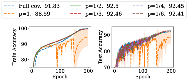
Figure 3: Train and test accuracy of ResNet-20 on CIFAR10 with varying value of $p$. Test accuracy values are indicated in the legends.

The same was also observed in Chen2018ClosingTG . When the network exhibits high activation variance, indicating strong responses to different inputs by individual neurons, AdaAct uses smaller optimization steps. Conversely, when the network has low activation variance, suggesting consistent neuron responses to inputs, it takes larger optimization steps. This emphasis on stable activations enhances overall neuron stability during training, fine-tuning the optimization process to accommodate individual neuron behavior.

Convolutional layer.

In CNNs, activations are 4D tensors of shape (batch(B), channel(C), height(H), width(W)). Viewing a convolution as a matrix-vector product, they are unfolded and reshaped into a 2D matrix by extracting patches at each spatial location and flattening into vectors, similar to im2col operation in GEMM-based implementation of convolution. There are $H\times W$ spatial locations and, for each location, we have a patch flattened into a vector of size $C\times\kappa\times\kappa$, where $\kappa$ is the size of kernel. This converts the convolution operations into matrix multiplications, enabling the application of our algorithm initially devised for fully connected layers to convolutional layers.

Hyperparameters.

Through a simple grid-based hyperparameter search, we discovered that our algorithm performs effectively with relatively high learning rates, typically around 0.1, while many other adaptive methods primarily use much smaller values, e.g., 0.001. Regarding weight decay, we adopt the decoupled weight decay Loshchilov2019DecoupledWD and recommend using the values smaller than the default 0.01 in AdamW. We observed that employing a higher weight decay value makes our algorithm converge similarly to SGD, achieving comparable generalization with it. Conversely, using a lower weight decay value enables fast convergence similar with Adam and its variants while still maintaining improved generalization.

5 Analysis of AdaAct

In this section, we analyze the convergence and generalization properties of AdaAct. For illustration purpose, we consider feed-forward networks consisting of linear layers, but our results can also be generalized to other types of layers.

5.1 Convergence Analysis

The convergence guarantee of AdaAct can be established using the framework due to chen2018on . For self-completeness, we provide a proof for the case in which the momentum factor $\beta_{1}$ is fixed i.e., $\beta_{1,t}=\beta_{1}$, for $\forall t$, in Appendix A. We make the following standard assumptions in stochastic optimization.

1. $f$ is differentiable and has $L$-Lipschitz gradient, i.e. $\forall\bm{\mathrm{x}},\bm{\mathrm{y}}$, $||\nabla{f(\bm{\mathrm{x}})}-\nabla{f(\bm{\mathrm{y}})}||_{2}\leq L||\bm{\mathrm{x}}-\bm{\mathrm{y}}||_{2}$. It is also lower bounded, i.e. $f(\bm{\mathrm{x}}^{*})>-\infty$ where $\bm{\mathrm{x}}^{*}$ is an optimal solution.

2. At time $t$, the algorithm can access a bounded noisy gradient and the true gradient is bounded, i.e. $||\nabla{f(\bm{\mathrm{\theta}}_{t})}||_{2}\leq H,\ ||\bm{\mathrm{g}}_{t}||_{2}\leq H,\ \forall t>1$.

3. The noisy gradient is unbiased and the noise is independent, i.e. $\bm{\mathrm{g}}_{t}=\nabla{f(\bm{\mathrm{\theta}}_{t})}+\bm{\mathrm{\zeta}}_{t},\ \operatorname{\mathbb{E}}[\bm{\mathrm{\zeta}}_{t}]=0$ and $\bm{\mathrm{\zeta}}_{i}$ is independent of $\bm{\mathrm{\zeta}}_{j}$ if $i\neq j$.

Theorem 5.1 (Theorem 3.1 in chen2018on ).

Suppose that assumptions A1-A3 are satisfied, $\beta_{1,t}=\beta_{1}$ for $\forall t$, and let $\gamma_{t}=\min_{j\in[d]}\min_{\{\bm{\mathrm{g}}_{i}\}_{i=1}^{t}}\frac{\eta_{t}}{\sqrt{\hat{\bm{\mathrm{v}}}_{t}}}$. Then we have

$$\min_{t\in[T]}\operatorname{\mathbb{E}}\left[\lVert\nabla{f}(\bm{\mathrm{x}}_{t})\rVert^{2}\right]$$

$$\leq\Biggl{\{}\operatorname{\mathbb{E}}\left[C_{1}\sum_{t=1}^{T}\left\lVert\frac{\eta_{1}\bm{\mathrm{g}}_{t}}{\sqrt{\hat{\bm{\mathrm{v}}}_{t}}}\right\rVert^{2}+C_{2}\sum_{t=2}^{T}\left\lVert\frac{\eta_{t}}{\sqrt{\hat{\bm{\mathrm{v}}}_{t}}}-\frac{\eta_{t-1}}{\sqrt{\hat{\bm{\mathrm{v}}}_{t-1}}}\right\rVert_{1}\right.$$

$$\quad\left.+C_{3}\sum_{t=2}^{T}\left\lVert\frac{\eta_{t}}{\sqrt{\hat{\bm{\mathrm{v}}}_{t}}}-\frac{\eta_{t-1}}{\sqrt{\hat{\bm{\mathrm{v}}}_{t-1}}}\right\rVert^{2}\right]+C_{4}\Biggr{\}}\Bigg{/}\sum_{t=1}^{T}\gamma_{t}\,,$$ (5)

where $C_{1},C_{2},C_{3}$ are constants independent of $d$ and $T$, $C_{4}$ is a constant independent of $T$, the expectation is taken with respect to all the randomness corresponding to $\{\bm{\mathrm{g}}_{t}\}$.

To compute the convergence rate for AdaAct, we make the following additional assumptions.

1. Activation variances are bounded, i.e. there exist constants $c_{L},\ c_{U}>0$ such that $c_{L}\leq(\tilde{\bm{\mathrm{a}}}_{t}^{2}\otimes\bm{\mathrm{1}})_{i}\leq c_{U},\ \forall t>1,$ and $\forall i\in[d]$ where $d=m_{\ell}(m_{\ell-1}+1)$.

2. For $\eta_{t}\leq\eta_{t-1}$, there exists $t_{0}>0$ such that $\sqrt{\widehat{\bm{\mathrm{v}}}_{t-1}/\widehat{\bm{\mathrm{v}}}_{t}}\leq\eta_{t-1}/\eta_{t}$ for $t\geq t_{0}$.

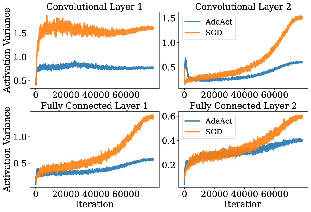
Figure 4: Activation variance resulted from training LeNet-5 on CIFAR10

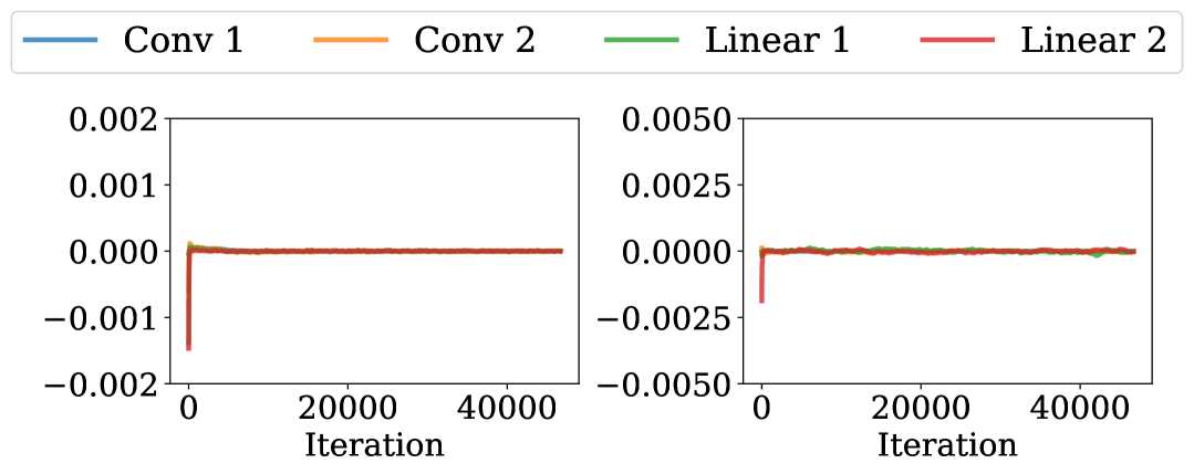
Figure 5: Difference in effective stepsizes: (Left) between iterations $\eta_{t}/\sqrt{\hat{v}_{t}}-\eta_{t-1}/\sqrt{\hat{v}_{t-1}}$, and (Right) between neighboring datasets $\eta/\sqrt{v_{t}}-\eta/\sqrt{v_{t}^{\prime}}$.

One way to satisfy Assumption A4 is to clip the estimated activation variances $\mathsf{Clip}(\bm{\mathrm{a}}_{t}^{2},c_{L},c_{U})$ to ensure the variances are in $[c_{L},c_{U}]$. However, we empirically observed that there exist natural lower and upper bound as AdaAct promotes stabilized activations. We trained LeNet-5 on CIFAR10 for 200 epochs to observe the trend of activation variance over iterations. Figure 5 presents the activation variances across all hidden layers in the architecture. We observe that the activations from layers are bounded.

Assumption A5 posits that the effective learning rates do not increase after a specific iteration $t_{0}$. This condition aligns mildly with the inherent behavior of adaptive methods such as AdaGrad and AMSGrad. Figure 5, generated using LeNet-5 on Fashion MNIST xiao2017fashionmnist illustrates in the left side that $\left(\eta_{t}/\sqrt{\widehat{\bm{\mathrm{v}}}_{t}}-\eta_{t-1}/\sqrt{\widehat{\bm{\mathrm{v}}}_{t-1}}\right)\to 0$, supporting the validity of Assumption A5. Assuming that the assumptions A1-A3 and Theorem 5.1 are satisfied, we present the following results.

Corollary 5.2.

If Assumption A4 and  A5 hold, for $\beta_{1}\in[0,1)$ and $\eta_{t}=1/\sqrt{t}$, AdaAct satisfies

$$\underset{t\in[T]}{\min}\operatorname{\mathbb{E}}\left[||f(\bm{\mathrm{\theta}}_{t})||^{2}\right]\leq\frac{1}{\sqrt{T}}\left(Q_{1}+Q_{2}\log{T}\right)$$ (6)

for any $T$, where $Q_{1}=\frac{c_{U}}{c_{L}^{2}}\left(C_{1}H^{2}+t_{0}d\left(c_{L}C_{2}+C_{3}\right)\right)+C_{4}$ and $Q_{2}=\frac{c_{U}C_{1}H^{2}}{c_{L}^{2}}$ are two constants independent of $T$.

The result in (6), in fact, indicates that AdaAct can achieve the same convergence rate $\mathcal{O}(\log{T}/\sqrt{T})$ as AMSGrad. See Appendix B for the proof.

5.2 Generalization Analysis

We bound the generalization error of AdaAct using the result of hardt2016Train on a connection between the generalization error and stability. Let $S=(z_{1},\ldots,z_{N})$ be a set of $N$ i.i.d. samples drawn from $\mathcal{D}$. The generalization error of model trained on $S$ using the randomized algorithm $\mathcal{A}$ is defined as

$$\epsilon_{\text{gen}}:=\operatorname{\mathbb{E}}_{S,\mathcal{A}}\left[\mathcal{R}_{S}(\mathcal{A}(S))-\mathcal{R}(\mathcal{A}(S))\right]\,,$$

where $\mathcal{R}_{S}$ and $\mathcal{R}$ denote the empirical and population risk, respectively.

Definition 5.3 (hardt2016Train ).

A randomized algorithm $\mathcal{A}$ is $\epsilon$-uniformly stable if for all pairs of datasets $S,S^{\prime}$ that differ in at most one example,

$$\sup_{\xi}\operatorname{\mathbb{E}}_{\mathcal{A}}\left[f(\mathcal{A}(S);\xi)-f(\mathcal{A}(S^{\prime});\xi)\right]\leq\epsilon\,.$$

Theorem 5.4 (hardt2016Train ).

Let $\mathcal{A}$ be an $\epsilon$-uniformly stable algorithm. Then we have $\lvert\epsilon_{\text{gen}}\rvert\leq\epsilon$.

Theorem 5.4 states that it suffices to prove that AdaAct is $\epsilon$-uniformly stable to bound its generalization error $\epsilon_{\text{gen}}$. Since the assumption A2 implies that the loss function $f$ is $H$-Lipschitz, it remains to show $\operatorname{\mathbb{E}}_{\mathcal{A}}\left[\left\lVert\bm{\mathrm{\theta}}_{t}-\bm{\mathrm{\theta}}_{t}^{\prime}\right\rVert_{2}\right]$ is bounded. Then we have $\sup_{\xi}\operatorname{\mathbb{E}}_{\mathcal{A}}\left[f(\mathcal{A}(S);\xi)-f(\mathcal{A}(S^{\prime});\xi)\right]\leq H\operatorname{\mathbb{E}}_{\mathcal{A}}\left[\left\lVert\bm{\mathrm{\theta}}_{t}-\bm{\mathrm{\theta}}_{t}^{\prime}\right\rVert_{2}\right]$.

Theorem 5.5.

Let $\bm{\mathrm{\theta}}_{t}$ (or $\bm{\mathrm{\theta}}_{t}^{\prime}$) be the parameter vector of model after being trained on $S$ (or $S^{\prime}$) for $t$ iterations using AdaAct with fixed learning rate $\eta$. Define $\Delta_{t}:=\lVert\bm{\mathrm{\theta}}_{t}-\bm{\mathrm{\theta}}_{t}^{\prime}\rVert_{2}$. Then we have

$$\operatorname{\mathbb{E}}\left[\Delta_{T+1}\right] \leq\frac{\eta H(N-1)}{N}\sum_{t=1}^{T}\underbracket{\operatorname{\mathbb{E}}{\left\lVert\frac{1}{\sqrt{\hat{\bm{\mathrm{v}}}_{t}}}-\frac{1}{\sqrt{\hat{\bm{\mathrm{v}}}_{t}^{\prime}}}\right\rVert_{2}}}_{A}$$

$$+\frac{\eta L}{c_{L}}\sum_{t=1}^{T}\underbracket{\operatorname{\mathbb{E}}\left[\sum_{k=1}^{t}\beta_{1}^{t-k}(1-\beta_{1})\Delta_{k}\right]}_{B}+\frac{2\eta HT}{Nc_{L}}\,.$$

As shown in Figure 5, the term $A$ in Theorem 5.5 is small enough (almost zero across iterations). The term $B$ is the EMA of $\Delta_{t}$ and the last term is small for datasets of moderate size. The generalization analysis demonstrates that AdaAct maintains a bounded generalization error, attributable to its $\epsilon$-uniform stability and the Lipschitz continuity of the loss function. See Appendix C for the proof.

6 Experiments

In this section, we evaluate AdaAct’s performance on the standard image classification task and compare it with other baselines. For comparisons, we trained ResNet he2016deep , DenseNet Huang2016DenselyCC , and Vision Transformer (ViT) dosovitskiy2021an on standard benchmark datasets: CIFAR10, CIFAR100, and ImageNet (ILSVRC 2012) deng2009imagenet . All experiments were performed using Nvidia Geforce RTX 3090 GPUs.

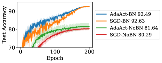
Figure 6: Test accuracy of ResNet-20 on CIFAR10: AdaAct generalizes better than SGD in the absence of batch normalization.

6.1 CIFAR Training Results

Training Settings.

We follow the settings for training the CIFAR datasets in Luo2019AdaBound and zhuang2020adabelief . Each network is trained for 200 epochs using the minibatch size of 128 with learning rate decayed according to the cosine annealing schedule. We used ResNet-20 and ResNet-32 for training CIFAR10 and ResNet-34 and DenseNet-121 for CIFAR100, and ran the experiments 5 times and report the mean and standard error for test accuracy to evaluate the generalization performance. We included state-of-the-art first- and second-order methods as baselines. Specifically, we chose SGD as a representative method for the class of first-order methods, Adam, AdamW, and Adan xie2023adan for the class of first-order adaptive methods, and KFAC and FOOF for the class of second-order methods. We conducted mild hyperparameter tuning specifically for Adan, FOOF, and KFAC. We varied the learning rate from 0.001 to 1.0, explored momentum and EMA coefficient values of 0.9, 0.95, and 0.99, and adjusted the damping factor between 0.01 and 10. For the remaining methods, we used the same settings as described in zhuang2020adabelief .

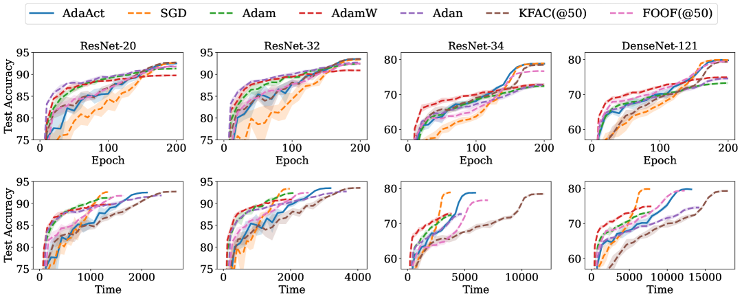
Figure 7: Comparison of test accuracy and training time among methods on CIFAR datasets

Table 1: Test accuracy (%) of ResNet and DenseNet on CIFAR datasets

Dataset	CIFAR10		CIFAR100
Architecture	ResNet-20	ResNet-32	ResNet-34	DenseNet-121
AdaAct	92.49$\pm$0.18	93.58$\pm$0.12	78.89$\pm$0.21	79.91$\pm$0.11
SGD	92.63$\pm$0.21	93.43$\pm$0.23	78.94$\pm$0.21	79.93$\pm$0.20
Adam	91.37$\pm$0.17	92.43$\pm$0.14	72.49$\pm$0.37	73.38$\pm$0.30
AdamW	89.85$\pm$0.21	90.99$\pm$0.21	72.87$\pm$0.46	74.99$\pm$0.20
Adan	91.87$\pm$0.16	92.77$\pm$0.15	72.83$\pm$0.54	74.65$\pm$0.43
KFAC	92.74$\pm$0.24	93.64$\pm$0.20	78.51$\pm$0.32	79.45$\pm$0.27
FOOF	91.79$\pm$0.09	92.50$\pm$0.16	76.79$\pm$0.09	79.44$\pm$0.18

Result.

To demonstrate the effect of activation variance adaption in AdaAct, we trained ResNet-20 models on CIFAR10 dataset with and without using batch normalization (BN) and presented the result in Figure 6. As shown, the removal of BN causes performance degradation for both AdaAct and SGD. However, we see that AdaAct is less affected by the removal. This is because that stabilized activations in AdaAct can create with BN to a certain extent.

Figure 7 shows the test accuracy of methods against iterations and wall-clock time. As shown in the graphs on the top row, the methods belonging to the adaptive gradient family (i.e., Adan, Adam, and AdamW) achieve higher test accuracy at early epochs and quickly reach the plateau around epoch 100. However, at the end of training, they end up achieving lower test accuracy than the other three algorithms: AdaAct, SGD, and KFAC (see Figure 7 and Table 1). This coincides with the observation made in prior work that adaptive gradient methods are faster in terms of convergence but suffer from poor generalization. While AdaAct is an adaptive methods, it achieves similar test accuracy with SGD and KFAC. This demonstrates the effectiveness of AdaAct’s activation variance-based adaptation in improving generalization performance. The graphs on the bottom row of Figure 7 shows that KFAC achieves the same accuracy with SGD and AdaAct, but it’s the slowest in terms of wall-clock time. FOOF and KFAC require computing the inverse of preconditioning matrix periodically and its frequency is controlled by the hyperparameter $T_{\text{inv}}$. We set $T_{\text{inv}}=50$ for both FOOF and KFAC. For CIFAR100, we observe that AdaAct converges as fast as Adam with training time similar to that of Adan — it is still significantly faster than FOOF and KFAC. This shows that AdaAct has an ability to match the generalization performance of KFAC while its speed is comparable to that of adaptive first-order algorithms.

6.2 ImageNet Training Results

Training Settings.

For ImageNet, we train ResNet-50, 101, and ViT-S networks, adopting the “A2” settings described in wightman2021resnet . It utilizes random crop, horizontal flip, Mixup (0.1) zhang2018mixup /CutMix (1.0) Yun2019CutMixRS with probability 0.5, and RandAugment Cubuk2019RandaugmentPA with $M=7$, $N=2$ and $MSTD=0.5$. It employs stochastic depth Huang2016DeepNW set at 0.05 and utilizes a cosine learning rate decay, in conjunction with a binary cross-entropy loss. For AdaAct, we used a template code from rw2019timm , setting a mini-batch size of 2,048 and cross-entropy loss is used for all architectures. We compare AdaAct with the baselines as previously reported by xie2023adan , but we omit the training results from Adan as they rely on micro fine-tuning. For both architectures, we used a large learning rate of 4.0, following the linear scaling rule as suggested in Goyal2017AccurateLM . We opted for a smaller weight decay value in ViT compared to ResNets to facilitate faster convergence, as its gradient per iteration significantly differs from that of CNNs due to a much sharper loss landscape Chen2021WhenVT .

Table 2: Top-1 accuracy (%) of ResNet-50 and 101 on ImageNet for 100 epochs. ^† are reported in xie2023adan

Architecture	ResNet-50	ResNet-101
AdaAct	77.6	79.4
SGD	77.0†	79.3†
Adam	76.9†	78.4†
AdamW	77.0†	78.9†
LAMB	77.0†	79.4†
SAM	77.3†	79.5†

Table 3: Top-1 accuracy (%) of ViT-S on ImageNet for 150 epochs. ^† are reported in xie2023adan

AdaAct	SGD	Adam	AdamW	LAMB
73.8	68.7†	64.0†	78.9†	73.8†

Result.

Table 2 demonstrate that AdaAct can provide good performance in large batch training setup (used in large-scale training). Specifically, AdaAct achieves the top-1 accuracy of 77.6% on ResNet-50, higher than other baseline methods, most of them showing the accuracy around 77.0%. For ResNet-101, AdaAct delivers competitive accuracy of 79.4%, matching the accuracy of LAMB You2020Large and is only slightly behind the performance of SAM foret2021sharpnessaware (79.5%), the best performer in this comparison but the slowest at the same time (due to the use of twice as many backprops as other methods). The fact that AdaAct surpasses Adam and LAMB, the methods-of-choice in practice for large-batch training, indicates its potential as an alternative in large-scale training. Table 3 presents the top-1 accuracy of ViT-S model on ImageNet dataset. In this experiment, AdaAct attains the top-1 accuracy of 73.8%, matching LAMB’s performance, which is significant given that LAMB is specifically designed for this setup and for Transformers Vaswani2017AttentionIA . Although AdaAct does not achieve the same accuracy with AdamW’s leading 78.9%, it still surpasses traditional methods such as SGD and Adam. This demonstrates AdaAct’s suitability and ability to handle particular optimization challenges for vision transformers. The fact that AdaAct outperforms SGD and Adam underscores its capability in navigating ViTs’ complex optimization landscape, which is notably different from that of CNNs. AdaAct’s comparable performance to LAMB, while still showing some gap from AdamW’s best performance, nevertheless marks it as a versatile optimization method potentially applicable across various architectures.

7 Conclusions

We presented AdaAct, an adaptive method designed to achieve improved generalization via stabilizing neuron outputs. Our approach focuses on adaptivity at the neuron level, promoting stable neuron responses even in the presence of varying activation variances. Beyond enhanced generalization, AdaAct introduces a fresh perspective on adapting learning rates based on activation variance, complementing existing activation regularization methods. In conclusion, AdaAct offers an effective solution to the challenges associated with adaptive optimization methods. Its improvements in generalization and network stability make it a valuable addition to the toolkit of deep learning practitioners.

Appendix A Proof of Theorem 5.1

Notice that AdaAct falls within the class of general Adam-type optimizer described in Algorithm 2. To see this, we rewrite the ${\bm{\mathrm{V}}}_{t}$ update in Line 5 of Algorithm 1 in a vector form. $\widehat{\bm{\mathrm{v}}}_{t}=\beta_{2}\widehat{\bm{\mathrm{v}}}_{t-1}+(1-\beta_{2})(\tilde{\bm{\mathrm{a}}}_{t}^{2}\otimes\bm{\mathrm{1}}_{m_{\ell}})$, where $\tilde{\bm{\mathrm{a}}}_{t}^{2}\otimes\bm{\mathrm{1}}_{m_{\ell}}=\bm{\mathrm{g}}_{t}^{2}/(\bm{\mathrm{1}}_{(m_{\ell-1}+1)}\otimes\bm{\mathrm{p}}_{t}^{2})$.

Algorithm 2 Generalized Adam

Initialize $\bm{\mathrm{m}}_{0}=0$ and $\bm{\mathrm{\theta}}_{1}$

1: for $t=1$ to $T$ do

2:  $\bm{\mathrm{m}}_{t}=\beta_{1,t}\bm{\mathrm{m}}_{t-1}+(1-\beta_{1,t})\bm{\mathrm{g}}_{t}$

3:  $\widehat{\bm{\mathrm{v}}}_{t}=h_{k}(\bm{\mathrm{g}}_{1},\bm{\mathrm{g}}_{2},\dots,\bm{\mathrm{g}}_{t})$

4:  $\bm{\mathrm{\theta}}_{t+1}=\bm{\mathrm{\theta}}_{t}-\eta_{t}\frac{\bm{\mathrm{m}}_{t}}{\sqrt{\widehat{\bm{\mathrm{v}}}_{t}}}$

5: end for

Lemma A.1.

Let $\bm{\mathrm{\theta}}_{0}:=\bm{\mathrm{\theta}}_{1}$ in Algorithm 2. Consider the sequence

$$\bm{\mathrm{z}}_{t}=\bm{\mathrm{\theta}}_{t}+\frac{\beta_{1}}{1-\beta_{1}}(\bm{\mathrm{\theta}}-\bm{\mathrm{\theta}}_{t-1})\,,\quad\forall t\geq 1\,.$$

Then we have

$$\bm{\mathrm{z}}_{t+1}-\bm{\mathrm{z}}_{t} =-\frac{\beta_{1}}{1-\beta_{1}}\left(\frac{\eta_{t}}{\sqrt{\hat{\bm{\mathrm{v}}}_{t}}}-\frac{\eta_{t-1}}{\sqrt{\hat{\bm{\mathrm{v}}}_{t-1}}}\right)\odot\bm{\mathrm{m}}_{t-1}-\eta_{t}\bm{\mathrm{g}}_{t}/\sqrt{\hat{\bm{\mathrm{v}}}_{t}}\,,\qquad\forall t>1\,,$$

and

$$\bm{\mathrm{z}}_{2}-\bm{\mathrm{z}}_{1} =-\frac{\eta_{1}\bm{\mathrm{m}}_{1}}{(1-\beta_{1})\sqrt{\hat{\bm{\mathrm{v}}}_{1}}}=-\frac{\eta_{1}\bm{\mathrm{g}}_{1}}{\sqrt{\hat{\bm{\mathrm{v}}}_{1}}}\,.$$

Proof.

$$\bm{\mathrm{\theta}}_{t+1}-\bm{\mathrm{\theta}}_{t} =-\eta_{t}\bm{\mathrm{m}}_{t}/\sqrt{\hat{\bm{\mathrm{v}}}_{t}}$$

$$=-\eta_{t}(\beta_{1}\bm{\mathrm{m}}_{t-1}+(1-\beta_{1})\bm{\mathrm{g}}_{t})\sqrt{\hat{\bm{\mathrm{v}}}_{t}}$$

$$=\beta_{1}\frac{\eta_{t}}{\eta_{t-1}}\frac{\sqrt{\hat{\bm{\mathrm{v}}}_{t-1}}}{\sqrt{\hat{\bm{\mathrm{v}}}_{t}}}\odot(\bm{\mathrm{\theta}}_{t}-\bm{\mathrm{\theta}}_{t-1})-\eta_{t}(1-\beta_{1})\bm{\mathrm{g}}_{t}/\sqrt{\hat{\bm{\mathrm{v}}}_{t}}$$

$$=\beta_{1}(\bm{\mathrm{\theta}}_{t}-\bm{\mathrm{\theta}}_{t-1})+\beta_{1}\left(\frac{\eta_{t}}{\eta_{t-1}}\frac{\sqrt{\hat{\bm{\mathrm{v}}}_{t-1}}}{\sqrt{\hat{\bm{\mathrm{v}}}_{t}}}-1\right)\odot(\bm{\mathrm{\theta}}_{t}-\bm{\mathrm{\theta}}_{t-1})-\eta_{t}(1-\beta_{1})\bm{\mathrm{g}}_{t}/\sqrt{\hat{\bm{\mathrm{v}}}_{t}}$$

$$=\beta_{1}(\bm{\mathrm{\theta}}_{t}-\bm{\mathrm{\theta}}_{t-1})+\beta_{1}\left(\frac{\eta_{t}}{\eta_{t-1}}\frac{\sqrt{\hat{\bm{\mathrm{v}}}_{t-1}}}{\sqrt{\hat{\bm{\mathrm{v}}}_{t}}}-1\right)\odot(-\eta_{t-1}\frac{\bm{\mathrm{m}}_{t-1}}{\sqrt{\hat{\bm{\mathrm{v}}}_{t-1}}})-\eta_{t}(1-\beta_{1})\bm{\mathrm{g}}_{t}/\sqrt{\hat{\bm{\mathrm{v}}}_{t}}$$

$$=\beta_{1}(\bm{\mathrm{\theta}}_{t}-\bm{\mathrm{\theta}}_{t-1})-\beta_{1}\left(\frac{\eta_{t}}{\sqrt{\hat{\bm{\mathrm{v}}}_{t}}}-\frac{\eta_{t-1}}{\sqrt{\hat{\bm{\mathrm{v}}}_{t-1}}}\right)\odot\bm{\mathrm{m}}_{t-1}-\eta_{t}(1-\beta_{1})\bm{\mathrm{g}}_{t}/\sqrt{\hat{\bm{\mathrm{v}}}_{t}}$$

Since $\bm{\mathrm{\theta}}_{t+1}-\bm{\mathrm{\theta}}_{t}=(1-\beta_{1})(\bm{\mathrm{\theta}}_{t+1}-\bm{\mathrm{\theta}}_{t})+\beta_{1}(\bm{\mathrm{\theta}}_{t+1}-\bm{\mathrm{\theta}}_{t})=(1-\beta_{1})\bm{\mathrm{\theta}}_{t+1}+\beta_{1}(\bm{\mathrm{\theta}}_{t+1}-\bm{\mathrm{\theta}}_{t})-(1-\beta_{1})\bm{\mathrm{\theta}}_{t}$, we have

$$(1-\beta_{1})\bm{\mathrm{\theta}}_{t+1}+\beta_{1}(\bm{\mathrm{\theta}}_{t+1}-\bm{\mathrm{\theta}}_{t})$$

$$=(1-\beta_{1})\bm{\mathrm{\theta}}_{t}+\beta_{1}(\bm{\mathrm{\theta}}_{t}-\bm{\mathrm{\theta}}_{t-1})-\beta_{1}\left(\frac{\eta_{t}}{\sqrt{\hat{\bm{\mathrm{v}}}_{t}}}-\frac{\eta_{t-1}}{\sqrt{\hat{\bm{\mathrm{v}}}_{t-1}}}\right)\odot\bm{\mathrm{m}}_{t-1}-\eta_{t}(1-\beta_{1})\bm{\mathrm{g}}_{t}/\sqrt{\hat{\bm{\mathrm{v}}}_{t}}$$

Dividing both sides by $$1-\beta_{1}$$ yields

$$\bm{\mathrm{\theta}}_{t+1}+\frac{\beta_{1}}{1-\beta_{1}}(\bm{\mathrm{\theta}}_{t+1}-\bm{\mathrm{\theta}}_{t})$$

$$=\bm{\mathrm{\theta}}_{t}+\frac{\beta_{1}}{1-\beta_{1}}(\bm{\mathrm{\theta}}_{t}-\bm{\mathrm{\theta}}_{t-1})-\frac{\beta_{1}}{1-\beta_{1}}\left(\frac{\eta_{t}}{\sqrt{\hat{\bm{\mathrm{v}}}_{t}}}-\frac{\eta_{t-1}}{\sqrt{\hat{\bm{\mathrm{v}}}_{t-1}}}\right)\odot\bm{\mathrm{m}}_{t-1}-\eta_{t}\bm{\mathrm{g}}_{t}/\sqrt{\hat{\bm{\mathrm{v}}}_{t}}\,.$$

Define the sequence

$$\bm{\mathrm{z}}_{t}=\bm{\mathrm{\theta}}_{t}+\frac{\beta_{1}}{1-\beta_{1}}(\bm{\mathrm{\theta}}_{t}-\bm{\mathrm{\theta}}_{t-1})\,.$$

Then we have

$$\bm{\mathrm{z}}_{t+1} =\bm{\mathrm{z}}_{t}-\frac{\beta_{1}}{1-\beta_{1}}\left(\frac{\eta_{t}}{\sqrt{\hat{\bm{\mathrm{v}}}_{t}}}-\frac{\eta_{t-1}}{\sqrt{\hat{\bm{\mathrm{v}}}_{t-1}}}\right)\odot\bm{\mathrm{m}}_{t-1}-\eta_{t}\bm{\mathrm{g}}_{t}/\sqrt{\hat{\bm{\mathrm{v}}}_{t}}\,,\forall t>1\,.$$

For $t=1$, we have $\bm{\mathrm{z}}_{1}=\bm{\mathrm{\theta}}_{1}$, and

$$\bm{\mathrm{z}}_{2}-\bm{\mathrm{z}}_{1} =\bm{\mathrm{\theta}}_{2}+\frac{\beta_{1}}{1-\beta_{1}}(\bm{\mathrm{\theta}}_{2}-\bm{\mathrm{\theta}}_{1})-\bm{\mathrm{\theta}}_{1}$$

$$=\frac{1}{1-\beta_{1}}(\bm{\mathrm{\theta}}_{2}-\bm{\mathrm{\theta}}_{1})$$

$$=-\frac{\eta_{1}\bm{\mathrm{m}}_{1}}{(1-\beta_{1})\sqrt{\hat{\bm{\mathrm{v}}}_{1}}}=-\frac{\eta_{1}\bm{\mathrm{g}}_{1}}{\sqrt{\hat{\bm{\mathrm{v}}}_{1}}}\,.$$

∎

Without loss of generality, we assume that Algorithm 2 is initialized such that

$$\left(\frac{\eta_{1}}{\sqrt{\hat{\bm{\mathrm{v}}}_{1}}}-\frac{\eta_{0}}{\hat{\bm{\mathrm{v}}}_{0}}\right)\odot\bm{\mathrm{m}}_{0}=\bm{\mathrm{0}}\,.$$ (7)

Lemma A.2.

Suppose that assumptions A1- A3 hold true. Then we have

$$\operatorname{\mathbb{E}}{f(\bm{\mathrm{z}}_{t+1})-f(\bm{\mathrm{z}}_{1})}\leq\sum_{i=1}^{4}T_{i}\,,$$

where

$$T_{1} =-\operatorname{\mathbb{E}}{\sum_{i=1}^{t}\left\langle\nabla{f}(\bm{\mathrm{z}}_{i}),\,\frac{\beta_{1}}{1-\beta_{1}}\left(\frac{\eta_{i}}{\sqrt{\hat{\bm{\mathrm{v}}}_{i}}}-\frac{\eta_{i-1}}{\sqrt{\hat{\bm{\mathrm{v}}}_{i-1}}}\right)\odot\bm{\mathrm{m}}_{i-1}\right\rangle}\,,$$ (8)

$$T_{2} =-\operatorname{\mathbb{E}}{\sum_{i=1}^{t}\left\langle\nabla{f}(\bm{\mathrm{z}}_{i}),\,\eta_{t}\bm{\mathrm{g}}_{i}/\sqrt{\hat{\bm{\mathrm{v}}}_{i}}\right\rangle}\,,$$ (9)

$$T_{3} =\operatorname{\mathbb{E}}{\sum_{i=1}^{t}L\left\lVert\frac{\beta_{1}}{1-\beta_{1}}\left(\frac{\eta_{i}}{\sqrt{\hat{\bm{\mathrm{v}}}_{i}}}-\frac{\eta_{i-1}}{\sqrt{\hat{\bm{\mathrm{v}}}_{i-1}}}\right)\odot\bm{\mathrm{m}}_{i-1}\right\rVert^{2}}\,,$$ (10)

$$T_{4} =\operatorname{\mathbb{E}}{\sum_{i=1}^{t}L\left\lVert\frac{\eta_{i}\bm{\mathrm{g}}_{i}}{\sqrt{\hat{\bm{\mathrm{v}}}_{i}}}\right\rVert^{2}}\,.$$ (11)

Proof.

By the smoothness of $\nabla{f}$, we have

$$f(\bm{\mathrm{z}}_{t+1})\leq f(\bm{\mathrm{z}}_{t})+\langle\nabla{f}(\bm{\mathrm{z}}_{t}),\,\bm{\mathrm{d}}_{t}\rangle+\frac{L}{2}\lVert\bm{\mathrm{d}}_{t}\rVert^{2}\,,$$

where $\bm{\mathrm{d}}_{t}=\bm{\mathrm{z}}_{t+1}-\bm{\mathrm{z}}_{t}$.

$$f(\bm{\mathrm{z}}_{i+1})-f(\bm{\mathrm{z}}_{i}) \leq\langle\nabla{f}(\bm{\mathrm{z}}_{i}),\,\bm{\mathrm{d}}_{i}\rangle+\frac{L}{2}\lVert\bm{\mathrm{d}}_{i}\rVert^{2}$$

From Lemma A.1, we have

$$=-\left\langle\nabla{f}(\bm{\mathrm{z}}_{i}),\,\frac{\beta_{1}}{1-\beta_{1}}\left(\frac{\eta_{t}}{\sqrt{\hat{\bm{\mathrm{v}}}_{t}}}-\frac{\eta_{t-1}}{\sqrt{\hat{\bm{\mathrm{v}}}_{t-1}}}\right)\odot\bm{\mathrm{m}}_{t-1}\right\rangle-\left\langle\nabla{f}(\bm{\mathrm{z}}_{i}),\,\eta_{t}\bm{\mathrm{g}}_{t}/\sqrt{\hat{\bm{\mathrm{v}}}_{t}}\right\rangle+\frac{L}{2}\lVert\bm{\mathrm{d}}_{i}\rVert^{2}$$

From the above, we get

$$\operatorname{\mathbb{E}}{f(\bm{\mathrm{z}}_{t+1})-f(\bm{\mathrm{z}}_{1})} =\operatorname{\mathbb{E}}{\sum_{i=1}^{t}f(\bm{\mathrm{z}}_{i+1})-f(\bm{\mathrm{z}}_{i})}$$

$$\leq-\operatorname{\mathbb{E}}{\sum_{i=1}^{t}\left\langle\nabla{f}(\bm{\mathrm{z}}_{i}),\,\frac{\beta_{1}}{1-\beta_{1}}\left(\frac{\eta_{i}}{\sqrt{\hat{\bm{\mathrm{v}}}_{i}}}-\frac{\eta_{i-1}}{\sqrt{\hat{\bm{\mathrm{v}}}_{i-1}}}\right)\odot\bm{\mathrm{m}}_{i-1}\right\rangle}$$

$$\qquad-\operatorname{\mathbb{E}}{\sum_{i=1}^{t}\left\langle\nabla{f}(\bm{\mathrm{z}}_{i}),\,\eta_{t}\bm{\mathrm{g}}_{i}/\sqrt{\hat{\bm{\mathrm{v}}}_{i}}\right\rangle}$$

$$\qquad+\operatorname{\mathbb{E}}{\sum_{i=1}^{t}\frac{L}{2}\left\lVert-\frac{\beta_{1}}{1-\beta_{1}}\left(\frac{\eta_{t}}{\sqrt{\hat{\bm{\mathrm{v}}}_{i}}}-\frac{\eta_{i-1}}{\sqrt{\hat{\bm{\mathrm{v}}}_{i-1}}}\right)\odot\bm{\mathrm{m}}_{i-1}-\frac{\eta_{t}\bm{\mathrm{g}}_{i}}{\sqrt{\hat{\bm{\mathrm{v}}}_{i}}}\right\rVert^{2}}$$

$$\leq-\operatorname{\mathbb{E}}{\sum_{i=1}^{t}\left\langle\nabla{f}(\bm{\mathrm{z}}_{i}),\,\frac{\beta_{1}}{1-\beta_{1}}\left(\frac{\eta_{i}}{\sqrt{\hat{\bm{\mathrm{v}}}_{i}}}-\frac{\eta_{i-1}}{\sqrt{\hat{\bm{\mathrm{v}}}_{i-1}}}\right)\odot\bm{\mathrm{m}}_{i-1}\right\rangle}$$

$$\qquad-\operatorname{\mathbb{E}}{\sum_{i=1}^{t}\left\langle\nabla{f}(\bm{\mathrm{z}}_{i}),\,\eta_{t}\bm{\mathrm{g}}_{i}/\sqrt{\hat{\bm{\mathrm{v}}}_{i}}\right\rangle}$$

$$\qquad+\operatorname{\mathbb{E}}{\sum_{i=1}^{t}L\left\lVert\frac{\beta_{1}}{1-\beta_{1}}\left(\frac{\eta_{i}}{\sqrt{\hat{\bm{\mathrm{v}}}_{i}}}-\frac{\eta_{i-1}}{\sqrt{\hat{\bm{\mathrm{v}}}_{i-1}}}\right)\odot\bm{\mathrm{m}}_{i-1}\right\rVert^{2}}+\operatorname{\mathbb{E}}{\sum_{i=1}^{t}L\left\lVert\frac{\eta_{i}\bm{\mathrm{g}}_{i}}{\sqrt{\hat{\bm{\mathrm{v}}}_{i}}}\right\rVert^{2}}$$

$$={\color[rgb]{1,0,0.5}T_{1}}+{\color[rgb]{0,0.75,0.16}T_{2}}+{\color[rgb]{1,0.58,0}T_{3}}+{\color[rgb]{0,0,1}T_{4}}\,,$$

where the last inequality is due to $\lVert\bm{\mathrm{a}}+\bm{\mathrm{b}}\rVert^{2}\leq 2\lVert\bm{\mathrm{a}}\rVert^{2}+2\lVert\bm{\mathrm{b}}\rVert^{2}$. ∎

Now, in the following series of lemmas, we bound each term in the above separately.

Lemma A.3.

Under the assumptions of A1- A3, we have

$${\color[rgb]{1,0,0.5}T_{1}} =-\operatorname{\mathbb{E}}{\sum_{i=1}^{t}\left\langle\nabla{f}(\bm{\mathrm{z}}_{i}),\,\frac{\beta_{1}}{1-\beta_{1}}\left(\frac{\eta_{t}}{\sqrt{\hat{\bm{\mathrm{v}}}_{t}}}-\frac{\eta_{t-1}}{\sqrt{\hat{\bm{\mathrm{v}}}_{t-1}}}\right)\odot\bm{\mathrm{m}}_{t-1}\right\rangle}$$

$$\leq H^{2}\frac{\beta_{1}}{1-\beta_{1}}\operatorname{\mathbb{E}}{\sum_{i=2}^{t}\sum_{j=1}^{d}\left\lvert\left(\frac{\eta_{i}}{\sqrt{\hat{\bm{\mathrm{v}}}_{i}}}-\frac{\eta_{i-1}}{\sqrt{\hat{\bm{\mathrm{v}}}_{i-1}}}\right)_{j}\right\rvert}\,.$$

Proof.

By the assumption A2, we have $\lVert\bm{\mathrm{g}}_{t}\rVert\leq H$. Since $\bm{\mathrm{m}}_{t}=\beta_{1}\bm{\mathrm{m}}_{t-1}+(1-\beta_{1})\bm{\mathrm{g}}_{t}$, we have $\lVert\bm{\mathrm{m}}_{t}\rVert\leq H$ (this can proved using a simple induction).

$$T_{1} =-\operatorname{\mathbb{E}}{\sum_{i=2}^{t}\left\langle\nabla{f}(\bm{\mathrm{z}}_{i}),\,\frac{\beta_{1}}{1-\beta_{1}}\left(\frac{\eta_{t}}{\sqrt{\hat{\bm{\mathrm{v}}}_{t}}}-\frac{\eta_{t-1}}{\sqrt{\hat{\bm{\mathrm{v}}}_{t-1}}}\right)\odot\bm{\mathrm{m}}_{t-1}\right\rangle}$$

$$\leq\operatorname{\mathbb{E}}{\sum_{i=2}^{t}\lVert\nabla{f}(\bm{\mathrm{z}}_{i})\rVert\lVert\bm{\mathrm{m}}_{i-1}\rVert\frac{\beta_{1}}{1-\beta_{1}}\sum_{j=1}^{d}\left\lvert\left(\frac{\eta_{i}}{\sqrt{\hat{\bm{\mathrm{v}}}_{i}}}-\frac{\eta_{i-1}}{\sqrt{\hat{\bm{\mathrm{v}}}_{i-1}}}\right)_{j}\right\rvert}$$

$$\leq H^{2}\frac{\beta_{1}}{1-\beta_{1}}\operatorname{\mathbb{E}}{\sum_{i=2}^{t}\sum_{j=1}^{d}\left\lvert\left(\frac{\eta_{i}}{\sqrt{\hat{\bm{\mathrm{v}}}_{i}}}-\frac{\eta_{i-1}}{\sqrt{\hat{\bm{\mathrm{v}}}_{i-1}}}\right)_{j}\right\rvert}\,.$$

In this above, we applied the Cauchy-Schwarz inequality to the first inequality, and the second inequality is due to the assumption of bounded gradient. ∎

Lemma A.4.

Suppose the assumptions A1- A3 hold. Then we have

$${\color[rgb]{0,0.75,0.16}T_{2}} =-\operatorname{\mathbb{E}}{\sum_{i=1}^{t}\left\langle\nabla{f}(\bm{\mathrm{z}}_{i}),\,\eta_{i}\bm{\mathrm{g}}_{i}/\sqrt{\hat{\bm{\mathrm{v}}}_{i}}\right\rangle}$$

$$\leq L^{2}\left(\frac{\beta_{1}}{1-\beta_{1}}\right)^{2}\operatorname{\mathbb{E}}{\sum_{i=1}^{t-1}\left\lVert\frac{\eta_{i}\bm{\mathrm{g}}_{i}}{\sqrt{\hat{\bm{\mathrm{v}}}_{i}}}\right\rVert^{2}}+L^{2}H^{2}\left(\frac{\beta_{1}}{1-\beta_{1}}\right)^{4}\operatorname{\mathbb{E}}{\sum_{j=1}^{d}\sum_{l=2}^{t-1}\left\lvert\frac{\eta_{l}}{\sqrt{\hat{\bm{\mathrm{v}}}_{l}}}-\frac{\eta_{l-1}}{\sqrt{\hat{\bm{\mathrm{v}}}_{l-1}}}\right\rvert_{j}^{2}}$$

$$\qquad+2H^{2}\operatorname{\mathbb{E}}{\sum_{i=2}^{t}\sum_{j=1}^{d}\left\lvert\left(\frac{\eta_{i}}{\sqrt{\hat{\bm{\mathrm{v}}}_{i}}}\right)_{j}-\left(\frac{\eta_{i-1}}{\sqrt{\hat{\bm{\mathrm{v}}}_{i-1}}}\right)_{j}\right\rvert}+2H^{2}\operatorname{\mathbb{E}}{\sum_{j=1}^{d}\left(\frac{\eta_{1}}{\hat{\bm{\mathrm{v}}}_{1}}\right)_{j}}$$

$$\qquad-\operatorname{\mathbb{E}}{\sum_{i=1}^{t}\eta_{i}\langle\nabla{f}(\bm{\mathrm{\theta}}_{i}),\,\nabla{f}(\bm{\mathrm{\theta}}_{i})/\sqrt{\hat{\bm{\mathrm{v}}}_{i}}\rangle}$$

$$\qquad+\frac{1}{2}\operatorname{\mathbb{E}}{\sum_{i=2}^{t}\left\lVert\frac{\eta_{i}\bm{\mathrm{g}}_{i}}{\sqrt{\hat{\bm{\mathrm{v}}}_{i}}}\right\rVert^{2}}\,.$$

Proof.

From the definition, we have

$$\bm{\mathrm{z}}_{i}-\bm{\mathrm{\theta}}_{i}=\frac{\beta_{1}}{1-\beta_{1}}(\bm{\mathrm{\theta}}_{i}-\bm{\mathrm{\theta}}_{i-1})=\frac{\beta_{1}}{1-\beta_{1}}\left(-\frac{\eta_{i-1}\bm{\mathrm{m}}_{i-1}}{\sqrt{\hat{\bm{\mathrm{v}}}_{i-1}}}\right)\text{ and }\bm{\mathrm{z}}_{1}=\bm{\mathrm{\theta}}_{1}\,.$$

Thus, we have

$$T_{2} =-\operatorname{\mathbb{E}}{\sum_{i=1}^{t}\eta_{i}\left\langle\nabla{f}(\bm{\mathrm{z}}_{i})+\nabla{f}(\bm{\mathrm{\theta}}_{i})-\nabla{f}(\bm{\mathrm{\theta}}_{i}),\,\frac{\bm{\mathrm{g}}_{i}}{\sqrt{\hat{\bm{\mathrm{v}}}_{i}}}\right\rangle}$$

$$=-\operatorname{\mathbb{E}}{\sum_{i=1}^{t}\eta_{i}\left\langle\nabla{f}(\bm{\mathrm{\theta}}_{i}),\,\frac{\bm{\mathrm{g}}_{i}}{\sqrt{\hat{\bm{\mathrm{v}}}_{i}}}\right\rangle}-\operatorname{\mathbb{E}}{\sum_{i=1}^{t}\eta_{i}\left\langle\nabla{f}(\bm{\mathrm{z}}_{i})-\nabla{f}(\bm{\mathrm{\theta}}_{i}),\,\frac{\bm{\mathrm{g}}_{i}}{\sqrt{\hat{\bm{\mathrm{v}}}_{i}}}\right\rangle}\,.$$

Applying $$\langle\bm{\mathrm{a}},\bm{\mathrm{b}}\rangle\leq\frac{1}{2}(\lVert\bm{\mathrm{a}}\rVert^{2}+\lVert\bm{\mathrm{b}}\rVert^{2})$$ to the second term yields

$$\leq-\operatorname{\mathbb{E}}{\sum_{i=1}^{t}\eta_{i}\left\langle\nabla{f}(\bm{\mathrm{\theta}}_{i}),\,\frac{\bm{\mathrm{g}}_{i}}{\sqrt{\hat{\bm{\mathrm{v}}}_{i}}}\right\rangle}+\operatorname{\mathbb{E}}{\sum_{i=2}^{t}\frac{1}{2}\lVert\nabla{f}(\bm{\mathrm{\theta}}_{i})-\nabla{f}(\bm{\mathrm{z}}_{i})\rVert^{2}+\frac{1}{2}\left\lVert\frac{\eta_{i}\bm{\mathrm{g}}_{i}}{\sqrt{\hat{\bm{\mathrm{v}}}_{i}}}\right\rVert^{2}}\,.$$

From the smoothness of $$\nabla{f}$$, we get

$$\leq-\operatorname{\mathbb{E}}{\sum_{i=1}^{t}\eta_{i}\left\langle\nabla{f}(\bm{\mathrm{\theta}}_{i}),\,\frac{\bm{\mathrm{g}}_{i}}{\sqrt{\hat{\bm{\mathrm{v}}}_{i}}}\right\rangle}+\frac{L^{2}}{2}\operatorname{\mathbb{E}}{\sum_{i=2}^{t}\left\lVert\frac{\beta_{1}}{1-\beta_{1}}\left(\frac{\eta_{i-1}\bm{\mathrm{m}}_{i-1}}{\sqrt{\hat{\bm{\mathrm{v}}}_{i-1}}}\right)\right\rVert^{2}}+\frac{1}{2}\operatorname{\mathbb{E}}{\sum_{i=2}^{t}\left\lVert\frac{\eta_{i}\bm{\mathrm{g}}_{i}}{\sqrt{\hat{\bm{\mathrm{v}}}_{i}}}\right\rVert^{2}}$$

$$=-T_{5}+\frac{L^{2}}{2}T_{6}+\frac{1}{2}T_{7}\,.$$

Bound on $T_{5}$.

The noisy gradient can be expressed as $\bm{\mathrm{g}}_{t}=\nabla{f}(\bm{\mathrm{\theta}}_{t})+\bm{\mathrm{\delta}}_{t}$ with $\operatorname{\mathbb{E}}{\bm{\mathrm{\delta}}_{t}}=\bm{\mathrm{0}}$.

$$T_{5} =\operatorname{\mathbb{E}}{\sum_{i=1}^{t}\eta_{i}\langle\nabla{f}(\bm{\mathrm{\theta}}_{i}),\,\bm{\mathrm{g}}_{i}/\sqrt{\hat{\bm{\mathrm{v}}}_{i}}\rangle}$$ (12)

$$=\operatorname{\mathbb{E}}{\sum_{i=1}^{t}\eta_{i}\langle\nabla{f}(\bm{\mathrm{\theta}}_{i}),\,(\nabla{f}(\bm{\mathrm{\theta}}_{i})+\bm{\mathrm{\delta}}_{i})/\sqrt{\hat{\bm{\mathrm{v}}}_{i}}\rangle}$$ (13)

$$=\operatorname{\mathbb{E}}{\sum_{i=1}^{t}\eta_{i}\langle\nabla{f}(\bm{\mathrm{\theta}}_{i}),\,\nabla{f}(\bm{\mathrm{\theta}}_{i})/\sqrt{\hat{\bm{\mathrm{v}}}_{i}}\rangle}+\operatorname{\mathbb{E}}{\sum_{i=1}^{t}\eta_{i}\langle\nabla{f}(\bm{\mathrm{\theta}}_{i}),\,\bm{\mathrm{\delta}}_{i}/\sqrt{\hat{\bm{\mathrm{v}}}_{i}}\rangle}$$ (14)

The second term in (14) can be bounded as follows.

$$\operatorname{\mathbb{E}}{\sum_{i=1}^{t}\eta_{i}\langle\nabla{f}(\bm{\mathrm{\theta}}_{i}),\,\bm{\mathrm{\delta}}_{i}/\sqrt{\hat{\bm{\mathrm{v}}}_{i}}\rangle}$$

$$=\operatorname{\mathbb{E}}{\sum_{i=2}^{t}\left\langle\nabla{f}(\bm{\mathrm{\theta}}_{i}),\,\bm{\mathrm{\delta}}_{i}\odot\left(\frac{\eta_{i}}{\sqrt{\hat{\bm{\mathrm{v}}}_{i}}}-\frac{\eta_{i-1}}{\sqrt{\hat{\bm{\mathrm{v}}}_{i-1}}}+\frac{\eta_{i-1}}{\sqrt{\hat{\bm{\mathrm{v}}}_{i-1}}}\right)\right\rangle}+\operatorname{\mathbb{E}}{\eta_{1}\left\langle\nabla{f}(\bm{\mathrm{\theta}}_{1}),\,\frac{\bm{\mathrm{\delta}}_{1}}{\hat{\bm{\mathrm{v}}}_{1}}\right\rangle}$$

$$\geq\operatorname{\mathbb{E}}{\sum_{i=2}^{t}\left\langle\nabla{f}(\bm{\mathrm{\theta}}_{i}),\,\bm{\mathrm{\delta}}_{i}\odot\left(\frac{\eta_{i}}{\sqrt{\hat{\bm{\mathrm{v}}}_{i}}}-\frac{\eta_{i-1}}{\sqrt{\hat{\bm{\mathrm{v}}}_{i-1}}}\right)\right\rangle}+\operatorname{\mathbb{E}}{\sum_{i=2}^{t}\left\langle\nabla{f}(\bm{\mathrm{\theta}}_{i}),\,\bm{\mathrm{\delta}}_{i}\odot\frac{\eta_{i-1}}{\sqrt{\hat{\bm{\mathrm{v}}}_{i-1}}}\right\rangle}-2H^{2}\operatorname{\mathbb{E}}{\sum_{j=1}^{d}\left(\frac{\eta_{1}}{\hat{\bm{\mathrm{v}}}_{1}}\right)_{j}}$$

Notice that given $$\bm{\mathrm{\theta}}_{i},\hat{\bm{\mathrm{v}}}_{i-1}$$ the expectation in the second term is 0.

$$=\operatorname{\mathbb{E}}{\sum_{i=2}^{t}\left\langle\nabla{f}(\bm{\mathrm{\theta}}_{i}),\,\bm{\mathrm{\delta}}_{i}\odot\left(\frac{\eta_{i}}{\sqrt{\hat{\bm{\mathrm{v}}}_{i}}}-\frac{\eta_{i-1}}{\sqrt{\hat{\bm{\mathrm{v}}}_{i-1}}}\right)\right\rangle}-2H^{2}\operatorname{\mathbb{E}}{\sum_{j=1}^{d}\left(\frac{\eta_{1}}{\hat{\bm{\mathrm{v}}}_{1}}\right)_{j}}$$ (15)

The first term in (14) can be bounded as

$$\operatorname{\mathbb{E}}{\sum_{i=2}^{t}\left\langle\nabla{f}(\bm{\mathrm{\theta}}_{i}),\,\bm{\mathrm{\delta}}_{i}\odot\left(\frac{\eta_{i}}{\sqrt{\hat{\bm{\mathrm{v}}}_{i}}}-\frac{\eta_{i-1}}{\sqrt{\hat{\bm{\mathrm{v}}}_{i-1}}}\right)\right\rangle}$$

$$=\operatorname{\mathbb{E}}{\sum_{i=2}^{t}\sum_{j=1}^{d}(\nabla{f}(\bm{\mathrm{\theta}}_{i}))_{j}\cdot(\bm{\mathrm{\delta}}_{i})_{j}\cdot\left(\left(\frac{\eta_{i}}{\sqrt{\hat{\bm{\mathrm{v}}}_{i}}}\right)_{j}-\left(\frac{\eta_{i-1}}{\sqrt{\hat{\bm{\mathrm{v}}}_{i-1}}}\right)_{j}\right)}$$

$$\geq-\operatorname{\mathbb{E}}{\sum_{i=2}^{t}\sum_{j=1}^{d}\left\lvert(\nabla{f}(\bm{\mathrm{\theta}}_{i}))_{j}\right\rvert\cdot\left\lvert(\bm{\mathrm{\delta}}_{i})_{j}\right\rvert\cdot\left\lvert\left(\frac{\eta_{i}}{\sqrt{\hat{\bm{\mathrm{v}}}_{i}}}\right)_{j}-\left(\frac{\eta_{i-1}}{\sqrt{\hat{\bm{\mathrm{v}}}_{i-1}}}\right)_{j}\right\rvert}$$

$$\geq-2H^{2}\operatorname{\mathbb{E}}{\sum_{i=2}^{t}\sum_{j=1}^{d}\left\lvert\left(\frac{\eta_{i}}{\sqrt{\hat{\bm{\mathrm{v}}}_{i}}}\right)_{j}-\left(\frac{\eta_{i-1}}{\sqrt{\hat{\bm{\mathrm{v}}}_{i-1}}}\right)_{j}\right\rvert}\,.$$ (16)

Applying (16) and (15) to (14) gives

$$-T_{5}=-\operatorname{\mathbb{E}}{\sum_{i=1}^{t}\eta_{i}\left\langle\nabla{f}(\bm{\mathrm{\theta}}_{i}),\,\frac{\bm{\mathrm{g}}_{i}}{\sqrt{\hat{\bm{\mathrm{v}}}_{i}}}\right\rangle} \leq 2H^{2}\operatorname{\mathbb{E}}{\sum_{i=2}^{t}\sum_{j=1}^{d}\left\lvert\left(\frac{\eta_{i}}{\sqrt{\hat{\bm{\mathrm{v}}}_{i}}}\right)_{j}-\left(\frac{\eta_{i-1}}{\sqrt{\hat{\bm{\mathrm{v}}}_{i-1}}}\right)_{j}\right\rvert}+2H^{2}\operatorname{\mathbb{E}}{\sum_{j=1}^{d}\left(\frac{\eta_{1}}{\hat{\bm{\mathrm{v}}}_{1}}\right)_{j}}$$

$$\qquad-\operatorname{\mathbb{E}}{\sum_{i=1}^{t}\eta_{i}\langle\nabla{f}(\bm{\mathrm{\theta}}_{i}),\,\nabla{f}(\bm{\mathrm{\theta}}_{i})/\sqrt{\hat{\bm{\mathrm{v}}}_{i}}\rangle}\,.$$ (17)

Bound on $T_{6}$.

By the update rule $\bm{\mathrm{m}}_{i}=\beta_{1}\bm{\mathrm{m}}_{i-1}+(1-\beta_{1})\bm{\mathrm{g}}_{i}$, we have $\bm{\mathrm{m}}_{i}=\sum_{k=1}^{i}\beta_{1}^{i-k}(1-\beta_{1})\bm{\mathrm{g}}_{k}$. From this, we have

$$T_{6} =\left(\frac{\beta_{1}}{1-\beta_{1}}\right)^{2}\operatorname{\mathbb{E}}{\sum_{i=2}^{t}\sum_{j=1}^{d}\left(\frac{\eta_{i-1}\bm{\mathrm{m}}_{i-1}}{\sqrt{\hat{\bm{\mathrm{v}}}_{i-1}}}\right)_{j}^{2}}$$

$$=\left(\frac{\beta_{1}}{1-\beta_{1}}\right)^{2}\operatorname{\mathbb{E}}{\sum_{i=2}^{t}\sum_{j=1}^{d}\left(\sum_{k=1}^{i-1}\frac{\eta_{i-1}\beta_{1}^{i-k-1}(1-\beta_{1})\bm{\mathrm{g}}_{k}}{\sqrt{\hat{\bm{\mathrm{v}}}_{i-1}}}\right)_{j}^{2}}$$

$$=\left(\frac{\beta_{1}}{1-\beta_{1}}\right)^{2}\operatorname{\mathbb{E}}{\sum_{i=2}^{t}\left\lVert\sum_{k=1}^{i-1}\frac{\eta_{k}\beta_{1}^{i-k-1}(1-\beta_{1})\bm{\mathrm{g}}_{k}}{\sqrt{\hat{\bm{\mathrm{v}}}_{k}}}+\beta_{1}^{i-k-1}(1-\beta_{1})\bm{\mathrm{g}}_{k}\left(\frac{\eta_{i-1}}{\sqrt{\hat{\bm{\mathrm{v}}}_{i-1}}}-\frac{\eta_{k}}{\sqrt{\hat{\bm{\mathrm{v}}}_{k}}}\right)\right\rVert^{2}}$$

$$\leq 2\beta_{1}^{2}\operatorname{\mathbb{E}}{\sum_{i=2}^{t}\left\lVert\sum_{k=1}^{i-1}\frac{\eta_{k}\beta_{1}^{i-k-1}\bm{\mathrm{g}}_{k}}{\sqrt{\hat{\bm{\mathrm{v}}}_{k}}}\right\rVert^{2}}+2\beta_{1}^{2}\operatorname{\mathbb{E}}{\sum_{i=2}^{t}\left\lVert\sum_{k=1}^{i-1}\beta_{1}^{i-k-1}\bm{\mathrm{g}}_{k}\left(\frac{\eta_{i-1}}{\sqrt{\hat{\bm{\mathrm{v}}}_{i-1}}}-\frac{\eta_{k}}{\sqrt{\hat{\bm{\mathrm{v}}}_{k}}}\right)\right\rVert^{2}}\,,$$ (18)

where the last inequality is due to $\lVert\bm{\mathrm{a}}+\bm{\mathrm{b}}\rVert^{2}\leq 2\lVert\bm{\mathrm{a}}\rVert^{2}+2\lVert\bm{\mathrm{b}}\rVert^{2}$. We bound the first term in (18).

$$\operatorname{\mathbb{E}}{\sum_{i=2}^{t}\left\lVert\sum_{k=1}^{i-1}\frac{\eta_{k}\beta_{1}^{i-k-1}\bm{\mathrm{g}}_{k}}{\sqrt{\hat{\bm{\mathrm{v}}}_{k}}}\right\rVert^{2}} =\operatorname{\mathbb{E}}{\sum_{i=2}^{t}\sum_{j=1}^{d}\sum_{p=1}^{i-1}\sum_{q=1}^{i-1}\beta_{1}^{i-p-1}\left(\frac{\eta_{p}\bm{\mathrm{g}}_{p}}{\sqrt{\hat{\bm{\mathrm{v}}}_{p}}}\right)_{j}\beta_{1}^{i-q-1}\left(\frac{\eta_{q}\bm{\mathrm{g}}_{q}}{\sqrt{\hat{\bm{\mathrm{v}}}_{q}}}\right)_{j}}$$

$$\leq\operatorname{\mathbb{E}}{\sum_{i=2}^{t}\sum_{j=1}^{d}\sum_{p=1}^{i-1}\sum_{q=1}^{i-1}\beta_{1}^{i-p-1}\beta_{1}^{i-q-1}\frac{1}{2}\left(\left(\frac{\eta_{p}\bm{\mathrm{g}}_{p}}{\sqrt{\hat{\bm{\mathrm{v}}}_{p}}}\right)_{j}^{2}+\left(\frac{\eta_{q}\bm{\mathrm{g}}_{q}}{\sqrt{\hat{\bm{\mathrm{v}}}_{q}}}\right)_{j}^{2}\right)}$$

By the symmetry of $$p q$$ and in the summation, we have

$$=\operatorname{\mathbb{E}}{\sum_{i=2}^{t}\sum_{j=1}^{d}\sum_{p=1}^{i-1}\left(\frac{\eta_{p}\bm{\mathrm{g}}_{p}}{\sqrt{\hat{\bm{\mathrm{v}}}_{p}}}\right)_{j}^{2}\beta_{1}^{i-p-1}\sum_{q=1}^{i-1}\beta_{1}^{i-q-1}}$$

$$=\frac{1}{1-\beta_{1}}\operatorname{\mathbb{E}}{\sum_{i=2}^{t}\sum_{j=1}^{d}\sum_{p=1}^{i-1}\beta_{1}^{i-p-1}\left(\frac{\eta_{p}\bm{\mathrm{g}}_{p}}{\sqrt{\hat{\bm{\mathrm{v}}}_{p}}}\right)_{j}^{2}}\,.$$

Changing the order of summation yields

$$=\frac{1}{1-\beta_{1}}\operatorname{\mathbb{E}}{\sum_{p=1}^{t-1}\sum_{j=1}^{d}\left(\frac{\eta_{p}\bm{\mathrm{g}}_{p}}{\sqrt{\hat{\bm{\mathrm{v}}}_{p}}}\right)_{j}^{2}\sum_{i=p+1}^{t}\beta_{1}^{i-p-1}}$$

$$\leq\left(\frac{1}{1-\beta_{1}}\right)^{2}\operatorname{\mathbb{E}}{\sum_{p=1}^{t-1}\sum_{j=1}^{d}\left(\frac{\eta_{p}\bm{\mathrm{g}}_{p}}{\sqrt{\hat{\bm{\mathrm{v}}}_{p}}}\right)_{j}^{2}}=\left(\frac{1}{1-\beta_{1}}\right)^{2}\operatorname{\mathbb{E}}{\sum_{i=1}^{t-1}\left\lVert\frac{\eta_{i}\bm{\mathrm{g}}_{i}}{\sqrt{\hat{\bm{\mathrm{v}}}_{i}}}\right\rVert^{2}}\,.$$ (19)

For the second term in (18), we have

$$\operatorname{\mathbb{E}}{\sum_{i=2}^{t}\left\lVert\sum_{k=1}^{i-1}\beta_{1}^{i-k-1}\bm{\mathrm{g}}_{k}\left(\frac{\eta_{i-1}}{\sqrt{\hat{\bm{\mathrm{v}}}_{i-1}}}-\frac{\eta_{k}}{\sqrt{\hat{\bm{\mathrm{v}}}_{k}}}\right)\right\rVert^{2}}$$

$$=\operatorname{\mathbb{E}}{\sum_{i=2}^{t}\sum_{j=1}^{d}\left(\sum_{k=1}^{i-1}\beta_{1}^{i-k-1}(\bm{\mathrm{g}}_{k})_{j}\left(\frac{\eta_{i-1}}{\sqrt{\hat{\bm{\mathrm{v}}}_{i-1}}}-\frac{\eta_{k}}{\sqrt{\hat{\bm{\mathrm{v}}}_{k}}}\right)_{j}\right)^{2}}$$

$$\leq H^{2}\operatorname{\mathbb{E}}{\sum_{i=2}^{t}\sum_{j=1}^{d}\left(\sum_{k=1}^{i-1}\beta_{1}^{i-k-1}\left\lvert\frac{\eta_{i-1}}{\sqrt{\hat{\bm{\mathrm{v}}}_{i-1}}}-\frac{\eta_{k}}{\sqrt{\hat{\bm{\mathrm{v}}}_{k}}}\right\rvert_{j}\right)^{2}}$$

$$=H^{2}\operatorname{\mathbb{E}}{\sum_{i=1}^{t-1}\sum_{j=1}^{d}\left(\sum_{k=1}^{i}\beta_{1}^{i-k}\left\lvert\frac{\eta_{i}}{\sqrt{\hat{\bm{\mathrm{v}}}_{i}}}-\frac{\eta_{k}}{\sqrt{\hat{\bm{\mathrm{v}}}_{k}}}\right\rvert_{j}\right)^{2}}$$

$$\leq H^{2}\operatorname{\mathbb{E}}{\sum_{i=1}^{t-1}\sum_{j=1}^{d}\left(\sum_{k=1}^{i}\beta_{1}^{i-k}\sum_{l=k+1}^{i}\left\lvert\frac{\eta_{l}}{\sqrt{\hat{\bm{\mathrm{v}}}_{l}}}-\frac{\eta_{l-1}}{\sqrt{\hat{\bm{\mathrm{v}}}_{l-1}}}\right\rvert_{j}\right)^{2}}$$

$$\leq H^{2}\left(\frac{1}{1-\beta_{1}}\right)^{2}\left(\frac{\beta_{1}}{1-\beta_{1}}\right)^{2}\operatorname{\mathbb{E}}{\sum_{j=1}^{d}\sum_{l=2}^{t-1}\left\lvert\frac{\eta_{l}}{\sqrt{\hat{\bm{\mathrm{v}}}_{l}}}-\frac{\eta_{l-1}}{\sqrt{\hat{\bm{\mathrm{v}}}_{l-1}}}\right\rvert_{j}^{2}}\,.$$ (20)

In the above, the last inequality is due to Lemma A.6.

From (19) and (20), we get

$$T_{6}\leq 2\left(\frac{\beta_{1}}{1-\beta_{1}}\right)^{2}\operatorname{\mathbb{E}}{\sum_{i=1}^{t-1}\left\lVert\frac{\eta_{i}\bm{\mathrm{g}}_{i}}{\sqrt{\hat{\bm{\mathrm{v}}}_{i}}}\right\rVert^{2}}+2H^{2}\left(\frac{\beta_{1}}{1-\beta_{1}}\right)^{4}\operatorname{\mathbb{E}}{\sum_{j=1}^{d}\sum_{l=2}^{t-1}\left\lvert\frac{\eta_{l}}{\sqrt{\hat{\bm{\mathrm{v}}}_{l}}}-\frac{\eta_{l-1}}{\sqrt{\hat{\bm{\mathrm{v}}}_{l-1}}}\right\rvert_{j}^{2}}$$ (21)

Combining (17) together with (21) gives the result. ∎

Lemma A.5.

Suppose the assumptions A1- A3 hold. Then we have

$${\color[rgb]{1,0.58,0}T_{3}} =\operatorname{\mathbb{E}}{\sum_{i=1}^{t}L\left\lVert\frac{\beta_{1}}{1-\beta_{1}}\left(\frac{\eta_{i}}{\sqrt{\hat{\bm{\mathrm{v}}}_{i}}}-\frac{\eta_{i-1}}{\sqrt{\hat{\bm{\mathrm{v}}}_{i-1}}}\right)\odot\bm{\mathrm{m}}_{i-1}\right\rVert^{2}}$$

$$\leq L\left(\frac{\beta_{1}}{1-\beta_{1}}\right)^{2}H^{2}\operatorname{\mathbb{E}}{\sum_{i=2}^{t}\sum_{j=1}^{d}\left(\frac{\eta_{i}}{\sqrt{\hat{\bm{\mathrm{v}}}_{i}}}-\frac{\eta_{i-1}}{\sqrt{\hat{\bm{\mathrm{v}}}_{i-1}}}\right)_{j}^{2}}$$

Proof.

$$\frac{1}{L}T_{3} =\operatorname{\mathbb{E}}{\sum_{i=2}^{t}\left(\frac{\beta_{1}}{1-\beta_{1}}\right)^{2}\sum_{j=1}^{d}\left(\frac{\eta_{i}}{\sqrt{\hat{\bm{\mathrm{v}}}_{i}}}-\frac{\eta_{i-1}}{\sqrt{\hat{\bm{\mathrm{v}}}_{i-1}}}\right)_{j}(\bm{\mathrm{m}}_{i-1})_{j}}$$

$$\leq\left(\frac{\beta_{1}}{1-\beta_{1}}\right)^{2}H^{2}\operatorname{\mathbb{E}}{\sum_{i=2}^{t}\sum_{j=1}^{d}\left(\frac{\eta_{i}}{\sqrt{\hat{\bm{\mathrm{v}}}_{i}}}-\frac{\eta_{i-1}}{\sqrt{\hat{\bm{\mathrm{v}}}_{i-1}}}\right)_{j}}\,,$$

where the last inequality is due to $\lVert\bm{\mathrm{m}}_{i}\rVert<H$. This completes the proof. ∎

Lemma A.6.

For $a_{i}\geq 0$, $\beta\in[0,1)$, and $b_{i}=\beta^{i-k}\sum_{l=k+1}^{i}a_{l}$, we have

$$\sum_{i=1}^{t}b_{i}^{2}\leq\left(\frac{1}{1-\beta}\right)^{2}\left(\frac{\beta}{1-\beta}\right)^{2}\sum_{i=2}^{t}a_{i}^{2}\,.$$

Proof.

We have

$$\sum_{i=1}^{t}b_{i}^{2} =\sum_{i=1}^{t}\left(\sum_{k-1}^{i}\beta^{i-k}\sum_{l=k+1}^{i}a_{l}\right)^{2}\,.$$

Changing the order of summation gives

$$=\sum_{i=1}^{t}\left(\sum_{l=2}^{i}\sum_{k=1}^{l-1}\beta^{i-k}a_{l}\right)^{2}=\sum_{i=1}^{t}\left(\sum_{l=2}^{i}\beta^{i-l+1}a_{l}\sum_{k=1}^{l-1}\beta^{l-1-k}\right)^{2}$$

$$\overset{(i)}{\leq}\left(\frac{1}{1-\beta}\right)^{2}\sum_{i=1}^{t}\left(\sum_{l=2}^{i}\beta^{i-l+1}a_{l}\right)^{2}=\left(\frac{1}{1-\beta}\right)^{2}\sum_{i=1}^{t}\left(\sum_{l=2}^{i}\sum_{m=2}^{i}\beta^{i-l+1}a_{l}\beta^{i-m+1}a_{m}\right)$$

$$\overset{(ii)}{\leq}\left(\frac{1}{1-\beta}\right)^{2}\sum_{i=1}^{t}\sum_{l=2}^{i}\sum_{m=2}^{i}\beta^{i-l+1}\beta^{i-m+1}\frac{1}{2}(a_{l}^{2}+a_{m}^{2})$$

$$\overset{(iii)}{=}\left(\frac{1}{1-\beta}\right)^{2}\sum_{i=1}^{t}\sum_{l=2}^{i}\sum_{m=2}^{i}\beta^{i-l+1}\beta^{i-m+1}a_{l}^{2}\leq\left(\frac{1}{1-\beta}\right)^{2}\frac{\beta}{1-\beta}\sum_{l=2}^{t}\sum_{i=l}^{t}\beta^{i-l+1}a_{l}^{2}$$

$$\leq\left(\frac{1}{1-\beta}\right)^{2}\left(\frac{\beta}{1-\beta}\right)^{2}\sum_{l=2}^{t}a_{l}^{2}\,,$$

where (i) used $\sum_{k=1}^{l-1-k}\leq\frac{1}{1-\beta}$, (ii) is due to $ab\leq\frac{1}{2}(a^{2}+b^{2})$, (iii) is due to symmetry of $l$ and $m$ in the summation. This completes the proof. ∎

Theorem A.7.

Suppose that the assumptions A1- A3 are satisfied and let $\gamma_{t}=\min_{j\in[d]}\min_{\{\bm{\mathrm{g}}_{i}\}_{i=1}^{t}}\frac{\eta_{t}}{\sqrt{\hat{\bm{\mathrm{v}}}_{t}}}$. Then we have

$$\min_{t\in[T]}\,\operatorname{\mathbb{E}}{\lVert\nabla{f}(\bm{\mathrm{\theta}}_{t})\rVert^{2}} \leq\frac{\operatorname{\mathbb{E}}{C_{1}\sum_{t=1}^{T}\lVert\frac{\eta_{1}\bm{\mathrm{g}}_{t}}{\sqrt{\hat{\bm{\mathrm{v}}}_{t}}}\rVert^{2}+C_{2}\sum_{t=2}^{T}\left\lVert\frac{\eta_{t}}{\sqrt{\hat{\bm{\mathrm{v}}}_{t}}}-\frac{\eta_{t-1}}{\sqrt{\hat{\bm{\mathrm{v}}}_{t-1}}}\right\rVert_{1}+C_{3}\sum_{t=2}^{T}\left\lVert\frac{\eta_{t}}{\sqrt{\hat{\bm{\mathrm{v}}}_{t}}}-\frac{\eta_{t-1}}{\sqrt{\hat{\bm{\mathrm{v}}}_{t-1}}}\right\rVert^{2}}+C_{4}}{\sum_{t=1}^{T}\gamma_{t}}\,.$$

Proof.

From Lemma A.2, we have

$$\operatorname{\mathbb{E}}{f(\bm{\mathrm{z}}_{t+1})-f(\bm{\mathrm{z}}_{1})} \leq\sum_{i=1}^{4}T_{i}$$

$$=-\operatorname{\mathbb{E}}{\sum_{i=1}^{t}\left\langle\nabla{f}(\bm{\mathrm{z}}_{i}),\,\frac{\beta_{1}}{1-\beta_{1}}\left(\frac{\eta_{i}}{\sqrt{\hat{\bm{\mathrm{v}}}_{i}}}-\frac{\eta_{i-1}}{\sqrt{\hat{\bm{\mathrm{v}}}_{i-1}}}\right)\odot\bm{\mathrm{m}}_{i-1}\right\rangle}\,,$$

$$\qquad-\operatorname{\mathbb{E}}{\sum_{i=1}^{t}\left\langle\nabla{f}(\bm{\mathrm{z}}_{i}),\,\eta_{t}\bm{\mathrm{g}}_{i}/\sqrt{\hat{\bm{\mathrm{v}}}_{i}}\right\rangle}\,,$$

$$\qquad+\operatorname{\mathbb{E}}{\sum_{i=1}^{t}L\left\lVert\frac{\beta_{1}}{1-\beta_{1}}\left(\frac{\eta_{i}}{\sqrt{\hat{\bm{\mathrm{v}}}_{i}}}-\frac{\eta_{i-1}}{\sqrt{\hat{\bm{\mathrm{v}}}_{i-1}}}\right)\odot\bm{\mathrm{m}}_{i-1}\right\rVert^{2}}\,,$$

$$\qquad+\operatorname{\mathbb{E}}{\sum_{i=1}^{t}L\left\lVert\frac{\eta_{i}\bm{\mathrm{g}}_{i}}{\sqrt{\hat{\bm{\mathrm{v}}}_{i}}}\right\rVert^{2}}$$

$$\leq H^{2}\frac{\beta_{1}}{1-\beta_{1}}\operatorname{\mathbb{E}}{\sum_{i=2}^{t}\sum_{j=1}^{d}\left\lvert\left(\frac{\eta_{i}}{\sqrt{\hat{\bm{\mathrm{v}}}_{i}}}-\frac{\eta_{i-1}}{\sqrt{\hat{\bm{\mathrm{v}}}_{i-1}}}\right)_{j}\right\rvert}$$

$$\qquad+L^{2}\left(\frac{\beta_{1}}{1-\beta_{1}}\right)^{2}\operatorname{\mathbb{E}}{\sum_{i=1}^{t-1}\left\lVert\frac{\eta_{i}\bm{\mathrm{g}}_{i}}{\sqrt{\hat{\bm{\mathrm{v}}}_{i}}}\right\rVert^{2}}+L^{2}H^{2}\left(\frac{\beta_{1}}{1-\beta_{1}}\right)^{4}\operatorname{\mathbb{E}}{\sum_{j=1}^{d}\sum_{l=2}^{t-1}\left\lvert\frac{\eta_{l}}{\sqrt{\hat{\bm{\mathrm{v}}}_{l}}}-\frac{\eta_{l-1}}{\sqrt{\hat{\bm{\mathrm{v}}}_{l-1}}}\right\rvert_{j}^{2}}$$

$$\qquad+2H^{2}\operatorname{\mathbb{E}}{\sum_{i=2}^{t}\sum_{j=1}^{d}\left\lvert\left(\frac{\eta_{i}}{\sqrt{\hat{\bm{\mathrm{v}}}_{i}}}\right)_{j}-\left(\frac{\eta_{i-1}}{\sqrt{\hat{\bm{\mathrm{v}}}_{i-1}}}\right)_{j}\right\rvert}+2H^{2}\operatorname{\mathbb{E}}{\sum_{j=1}^{d}\left(\frac{\eta_{1}}{\hat{\bm{\mathrm{v}}}_{1}}\right)_{j}}$$

$$\qquad-\operatorname{\mathbb{E}}{\sum_{i=1}^{t}\eta_{i}\langle\nabla{f}(\bm{\mathrm{\theta}}_{i}),\,\nabla{f}(\bm{\mathrm{\theta}}_{i})/\sqrt{\hat{\bm{\mathrm{v}}}_{i}}\rangle}+\frac{1}{2}\operatorname{\mathbb{E}}{\sum_{i=2}^{t}\left\lVert\frac{\eta_{i}\bm{\mathrm{g}}_{i}}{\sqrt{\hat{\bm{\mathrm{v}}}_{i}}}\right\rVert^{2}}$$

$$\qquad+L\left(\frac{\beta_{1}}{1-\beta_{1}}\right)^{2}H^{2}\operatorname{\mathbb{E}}{\sum_{i=2}^{t}\sum_{j=1}^{d}\left(\frac{\eta_{i}}{\sqrt{\hat{\bm{\mathrm{v}}}_{i}}}-\frac{\eta_{i-1}}{\sqrt{\hat{\bm{\mathrm{v}}}_{i-1}}}\right)_{j}}$$

$$\qquad+\operatorname{\mathbb{E}}{\sum_{i=1}^{t}L\left\lVert\frac{\eta_{i}\bm{\mathrm{g}}_{i}}{\sqrt{\hat{\bm{\mathrm{v}}}_{i}}}\right\rVert^{2}}\,.$$

By merging similar terms, we get

$$\leq\left(H^{2}\frac{\beta_{1}}{1-\beta_{1}}+2H^{2}\right)\operatorname{\mathbb{E}}{\sum_{i=2}^{t}\sum_{j=1}^{d}\left\lvert\left(\frac{\eta_{i}}{\sqrt{\hat{\bm{\mathrm{v}}}_{i}}}-\frac{\eta_{i-1}}{\sqrt{\hat{\bm{\mathrm{v}}}_{i-1}}}\right)_{j}\right\rvert}$$

$$\qquad+\left(1+L\left(\frac{\beta_{1}}{1-\beta_{1}}\right)^{2}\right)LH^{2}\left(\frac{\beta_{1}}{1-\beta_{1}}\right)^{2}\operatorname{\mathbb{E}}{\sum_{j=1}^{d}\sum_{i=2}^{t}\left(\frac{\eta_{i}}{\sqrt{\hat{\bm{\mathrm{v}}}_{i}}}-\frac{\eta_{i-1}}{\sqrt{\hat{\bm{\mathrm{v}}}_{i-1}}}\right)_{j}^{2}}$$

$$\qquad+\left(L^{2}\left(\frac{\beta_{1}}{1-\beta_{1}}\right)^{2}+\frac{1}{2}+L\right)\operatorname{\mathbb{E}}{\sum_{i=1}^{t}\left\lVert\frac{\eta_{i}\bm{\mathrm{g}}_{i}}{\sqrt{\hat{\bm{\mathrm{v}}}_{i}}}\right\rVert^{2}}$$

$$\qquad+2H^{2}\operatorname{\mathbb{E}}{\sum_{j=1}^{d}\left(\frac{\eta_{1}}{\hat{\bm{\mathrm{v}}}_{1}}\right)_{j}}-\operatorname{\mathbb{E}}{\sum_{i=1}^{t}\eta_{i}\langle\nabla{f}(\bm{\mathrm{\theta}}_{i}),\,\nabla{f}(\bm{\mathrm{\theta}}_{i})/\sqrt{\hat{\bm{\mathrm{v}}}_{i}}\rangle}\,.$$

Rearranging terms gives

$$\operatorname{\mathbb{E}}{\sum_{i=1}^{t}\langle\nabla{f}(\bm{\mathrm{\theta}}_{i}),\,\frac{\eta_{i}\nabla{f}(\bm{\mathrm{\theta}}_{i})}{\sqrt{\hat{\bm{\mathrm{v}}}_{i}}}\rangle}$$

$$\leq\left(H^{2}\frac{\beta_{1}}{1-\beta_{1}}+2H^{2}\right)\operatorname{\mathbb{E}}{\sum_{i=2}^{t}\sum_{j=1}^{d}\left\lvert\left(\frac{\eta_{i}}{\sqrt{\hat{\bm{\mathrm{v}}}_{i}}}-\frac{\eta_{i-1}}{\sqrt{\hat{\bm{\mathrm{v}}}_{i-1}}}\right)_{j}\right\rvert}$$

$$\qquad+\left(1+L\left(\frac{\beta_{1}}{1-\beta_{1}}\right)^{2}\right)LH^{2}\left(\frac{\beta_{1}}{1-\beta_{1}}\right)^{2}\operatorname{\mathbb{E}}{\sum_{j=1}^{d}\sum_{i=2}^{t}\left(\frac{\eta_{i}}{\sqrt{\hat{\bm{\mathrm{v}}}_{i}}}-\frac{\eta_{i-1}}{\sqrt{\hat{\bm{\mathrm{v}}}_{i-1}}}\right)_{j}^{2}}$$

$$\qquad+\left(L^{2}\left(\frac{\beta_{1}}{1-\beta_{1}}\right)^{2}+\frac{1}{2}+L\right)\operatorname{\mathbb{E}}{\sum_{i=1}^{t}\left\lVert\frac{\eta_{i}\bm{\mathrm{g}}_{i}}{\sqrt{\hat{\bm{\mathrm{v}}}_{i}}}\right\rVert^{2}}+2H^{2}\operatorname{\mathbb{E}}{\sum_{j=1}^{d}\left(\frac{\eta_{1}}{\hat{\bm{\mathrm{v}}}_{1}}\right)_{j}}$$

$$\qquad+\operatorname{\mathbb{E}}{f(\bm{\mathrm{z}}_{1})-f(\bm{\mathrm{z}}_{t+1})}$$

$$\leq C_{1}\operatorname{\mathbb{E}}{\sum_{i=1}^{t}\left\lVert\frac{\eta_{i}\bm{\mathrm{g}}_{i}}{\sqrt{\hat{\bm{\mathrm{v}}}_{i}}}\right\rVert^{2}}+C_{2}\operatorname{\mathbb{E}}{\sum_{i=2}^{t}\left\lVert\frac{\eta_{i}}{\sqrt{\hat{\bm{\mathrm{v}}}_{i}}}-\frac{\eta_{i-1}}{\sqrt{\hat{\bm{\mathrm{v}}}_{i-1}}}\right\rVert_{1}}+C_{3}\operatorname{\mathbb{E}}{\sum_{i=2}^{t}\left\lVert\frac{\eta_{i}}{\sqrt{\hat{\bm{\mathrm{v}}}_{i}}}-\frac{\eta_{i-1}}{\sqrt{\hat{\bm{\mathrm{v}}}_{i-1}}}\right\rVert^{2}}+C_{4}\,,$$

where

$$C_{1} =\left(L^{2}\left(\frac{\beta_{1}}{1-\beta_{1}}\right)^{2}+\frac{1}{2}+L\right)\,,$$

$$C_{2} =\left(H^{2}\frac{\beta_{1}}{1-\beta_{1}}+2H^{2}\right)\,,$$

$$C_{3} =\left(1+L\left(\frac{\beta_{1}}{1-\beta_{1}}\right)^{2}\right)LH^{2}\left(\frac{\beta_{1}}{1-\beta_{1}}\right)^{2}\,,$$

$$C_{4} =2H^{2}\operatorname{\mathbb{E}}{\sum_{j=1}^{d}\left(\frac{\eta_{1}}{\hat{\bm{\mathrm{v}}}_{1}}\right)_{j}}+\operatorname{\mathbb{E}}{f(\bm{\mathrm{z}}_{1})-f(\bm{\mathrm{z}}^{*})}\,.$$

From the above, we have

$$\operatorname{\mathbb{E}}{\sum_{t=1}^{T}\langle\nabla{f}(\bm{\mathrm{\theta}}_{t}),\,\frac{\eta_{t}\nabla{f}(\bm{\mathrm{\theta}}_{t})}{\sqrt{\hat{\bm{\mathrm{v}}}_{t}}}\rangle} \geq\operatorname{\mathbb{E}}{\sum_{t=1}^{T}\gamma_{t}\lVert\nabla{f}(\bm{\mathrm{\theta}}_{t})\rVert^{2}}$$

$$\geq\min_{t\in[T]}\,\operatorname{\mathbb{E}}{\lVert\nabla{f}(\bm{\mathrm{\theta}}_{t})\rVert^{2}}\sum_{t=1}^{T}\gamma_{t}\,.$$

Thus, we have

$$\min_{t\in[T]}\,\operatorname{\mathbb{E}}{\lVert\nabla{f}(\bm{\mathrm{\theta}}_{t})\rVert^{2}} \leq\frac{\operatorname{\mathbb{E}}{C_{1}\sum_{t=1}^{T}\lVert\frac{\eta_{1}\bm{\mathrm{g}}_{t}}{\sqrt{\hat{\bm{\mathrm{v}}}_{t}}}\rVert^{2}+C_{2}\sum_{t=2}^{T}\left\lVert\frac{\eta_{t}}{\sqrt{\hat{\bm{\mathrm{v}}}_{t}}}-\frac{\eta_{t-1}}{\sqrt{\hat{\bm{\mathrm{v}}}_{t-1}}}\right\rVert_{1}+C_{3}\sum_{t=2}^{T}\left\lVert\frac{\eta_{t}}{\sqrt{\hat{\bm{\mathrm{v}}}_{t}}}-\frac{\eta_{t-1}}{\sqrt{\hat{\bm{\mathrm{v}}}_{t-1}}}\right\rVert^{2}}+C_{4}}{\sum_{t=1}^{T}\gamma_{t}}\,.$$

∎

Appendix B Proof of Corollary 5.2

Proof.

We first bound non-constant terms in RHS of (5.1). For the term with $C_{1}$, we have

$$\operatorname{\mathbb{E}}\left[\sum_{t=1}^{T}\left\|\eta_{t}\bm{\mathrm{g}}_{t}/\sqrt{\widehat{\bm{\mathrm{v}}}_{t}}\right\|^{2}\right] \leq\operatorname{\mathbb{E}}\left[\sum_{t=1}^{T}\left\|\eta_{t}\bm{\mathrm{g}}_{t}/c_{L}\right\|^{2}\right]\quad\text{by Assumption~\ref{as:1}}$$

$$=\operatorname{\mathbb{E}}\left[\sum_{t=1}^{T}\left(\frac{1}{c_{L}\sqrt{t}}\right)^{2}\left\|\bm{\mathrm{g}}_{t}\right\|^{2}\right]$$

$$\leq\frac{H^{2}}{c_{L}^{2}}\sum_{t=1}^{T}\frac{1}{t}$$

$$\leq\frac{H^{2}}{c_{L}^{2}}(1+\log{T})\,,$$

where the last inequality is due to $\sum_{t=1}^{T}\frac{1}{t}\leq 1+\log T$.

For the term with $C_{2}$, we have

$$\operatorname{\mathbb{E}}\left[\sum_{t=2}^{T}\left\|\frac{\eta_{t}}{\sqrt{\widehat{\bm{\mathrm{v}}}_{t}}}-\frac{\eta_{t-1}}{\sqrt{\widehat{\bm{\mathrm{v}}}_{t-1}}}\right\|_{1}\right]$$

$$=\operatorname{\mathbb{E}}\left[\sum_{t=2}^{t_{0}}\left\|\frac{\eta_{t}}{\sqrt{\widehat{\bm{\mathrm{v}}}_{t}}}-\frac{\eta_{t-1}}{\sqrt{\widehat{\bm{\mathrm{v}}}_{t-1}}}\right\|_{1}+\sum_{t=t_{0}+1}^{T}\left\|\frac{\eta_{t}}{\sqrt{\widehat{\bm{\mathrm{v}}}_{t}}}-\frac{\eta_{t-1}}{\sqrt{\widehat{\bm{\mathrm{v}}}_{t-1}}}\right\|_{1}\right]$$

$$=\operatorname{\mathbb{E}}\left[\sum_{t=2}^{t_{0}}\sum_{j=1}^{d}\left|\frac{\eta_{t}}{(\sqrt{\widehat{\bm{\mathrm{v}}}_{t}})_{j}}-\frac{\eta_{t-1}}{(\sqrt{\widehat{\bm{\mathrm{v}}}_{t-1}})_{j}}\right|+\sum_{j=1}^{d}\sum_{t=t_{0}+1}^{T}\left(\frac{\eta_{t-1}}{(\sqrt{\widehat{\bm{\mathrm{v}}}_{t-1}})_{j}}-\frac{\eta_{t}}{(\sqrt{\widehat{\bm{\mathrm{v}}}_{t}})_{j}}\right)\right]\quad\text{by Assumption~\ref{as:2}}$$

$$\leq\operatorname{\mathbb{E}}\left[\sum_{t=2}^{t_{0}}\frac{d}{c_{L}}+\sum_{j=1}^{d}\left(\frac{\eta_{t_{0}}}{(\sqrt{\widehat{\bm{\mathrm{v}}}_{t_{0}})_{j}}}-\frac{\eta_{T}}{(\sqrt{\widehat{\bm{\mathrm{v}}}_{T}})_{j}}\right)\right]$$

$$=\frac{t_{0}d}{c_{L}},$$

where $\left|\eta_{t}/(\sqrt{\widehat{\bm{\mathrm{v}}}_{t}})_{j}-\eta_{t-1}/(\sqrt{\widehat{\bm{\mathrm{v}}}_{t-1}})_{j}\right|\leq 1/c_{L}$.

For the term with $C_{3}$, we have

$$\operatorname{\mathbb{E}}\left[\sum_{t=2}^{T-1}\left\|\frac{\eta_{t}}{\sqrt{\widehat{\bm{\mathrm{v}}}_{t}}}-\frac{\eta_{t-1}}{\sqrt{\widehat{\bm{\mathrm{v}}}_{t-1}}}\right\|^{2}\right] =\operatorname{\mathbb{E}}\left[\sum_{t=2}^{t_{0}}\left\|\frac{\eta_{t}}{\sqrt{\widehat{\bm{\mathrm{v}}}_{t}}}-\frac{\eta_{t-1}}{\sqrt{\widehat{\bm{\mathrm{v}}}_{t-1}}}\right\|^{2}+\sum_{t=t_{0}+1}^{T}\left\|\frac{\eta_{t}}{\sqrt{\widehat{\bm{\mathrm{v}}}_{t}}}-\frac{\eta_{t-1}}{\sqrt{\widehat{\bm{\mathrm{v}}}_{t-1}}}\right\|^{2}\right]$$

$$\leq\operatorname{\mathbb{E}}\left[\frac{1}{c}\left(\sum_{t=2}^{t_{0}}\left\|\frac{\eta_{t}}{\sqrt{\widehat{\bm{\mathrm{v}}}_{t}}}-\frac{\eta_{t-1}}{\sqrt{\widehat{\bm{\mathrm{v}}}_{t-1}}}\right\|_{1}+\sum_{t=t_{0}+1}^{T}\left\|\frac{\eta_{t}}{\sqrt{\widehat{\bm{\mathrm{v}}}_{t}}}-\frac{\eta_{t-1}}{\sqrt{\widehat{\bm{\mathrm{v}}}_{t-1}}}\right\|_{1}\right)\right]$$

$$\leq\frac{1}{c_{L}}\left(\frac{(t_{0}-1)d}{c_{L}}+\frac{d}{c_{L}}\right)$$

$$=\frac{t_{0}d}{c_{L}^{2}}.$$

Then we have for AdaAct,

$$\operatorname{\mathbb{E}}\left[C_{1}\sum_{t=1}^{T}\left\|\eta_{t}\bm{\mathrm{g}}_{t}/\sqrt{\widehat{\bm{\mathrm{v}}}_{t}}\right\|^{2}+C_{2}\sum_{t=2}^{T}\left\|\frac{\eta_{t}}{\sqrt{\widehat{\bm{\mathrm{v}}}_{t}}}-\frac{\eta_{t-1}}{\sqrt{\widehat{\bm{\mathrm{v}}}_{t-1}}}\right\|_{1}+C_{3}\sum_{t=2}^{T-1}\left\|\frac{\eta_{t}}{\sqrt{\widehat{\bm{\mathrm{v}}}_{t}}}-\frac{\eta_{t-1}}{\sqrt{\widehat{\bm{\mathrm{v}}}_{t-1}}}\right\|^{2}\right]+C_{4}$$

$$\leq\frac{C_{1}H^{2}}{c_{L}^{2}}(1+\log{T})+\frac{C_{2}t_{0}d}{c_{L}}+\frac{C_{3}t_{0}d}{c_{L}^{2}}+C_{4}.$$ (22)

Now we lower bound the effective stepsizes by Assumption A4,

$$\frac{\eta_{t}}{(\sqrt{\widehat{\bm{\mathrm{v}}}_{t}})_{j}}\geq\frac{1}{c_{U}\sqrt{t}}.$$

Thus,

$$\operatorname{\mathbb{E}}\left[\sum_{t=1}^{T}\eta_{t}\langle\nabla{f(\bm{\mathrm{\theta}}_{t})},\ \nabla{f(\bm{\mathrm{\theta}}_{t})}/\sqrt{\widehat{\bm{\mathrm{v}}}_{t}}\rangle\right]\geq\operatorname{\mathbb{E}}\left[\sum_{t=1}^{T}\frac{1}{c_{U}\sqrt{t}}\left\|\nabla{f(\bm{\mathrm{\theta}}_{t})}\right\|^{2}\right]\geq\frac{\sqrt{T}}{c_{U}}\underset{t\in[T]}{\min}{\operatorname{\mathbb{E}}\left[\left\|\nabla{f(\bm{\mathrm{\theta}}_{t})}\right\|^{2}\right]}.$$ (23)

Then by (5.1), (B), and (23), we have

$$\frac{\sqrt{T}}{c_{U}}\underset{t\in[T]}{\min}{\operatorname{\mathbb{E}}\left[\left\|\nabla{f(\bm{\mathrm{\theta}}_{t})}\right\|^{2}\right]}\leq\frac{C_{1}H^{2}}{c_{L}^{2}}(1+\log{T})+\frac{C_{2}t_{0}d}{c_{L}}+\frac{C_{3}t_{0}d}{c_{L}^{2}}+C_{4}$$

which is equivalent to

$$\underset{t\in[T]}{\min}{\operatorname{\mathbb{E}}\left[\left\|\nabla{f(\bm{\mathrm{\theta}}_{t})}\right\|^{2}\right]} \leq\frac{c_{U}}{\sqrt{T}}\left(\frac{C_{1}H^{2}}{c_{L}^{2}}(1+\log{T})+\frac{C_{2}t_{0}d}{c_{L}}+\frac{C_{3}t_{0}d}{c_{L}^{2}}+C_{4}\right)$$

$$=\frac{1}{\sqrt{T}}\left(Q_{1}+Q_{2}\log{T}\right).$$

∎

Appendix C Proof of Theorem 5.5

By definition, we have

$$\operatorname{\mathbb{E}}\left[\Delta_{T+1}\right] =\operatorname{\mathbb{E}}\left[\lVert\bm{\mathrm{\theta}}_{T+1}-\bm{\mathrm{\theta}}_{T+1}^{\prime}\rVert_{2}\right]$$

$$=\operatorname{\mathbb{E}}{\left\lVert\bm{\mathrm{\theta}}_{1}-\sum_{t=1}^{T}\frac{\eta\bm{\mathrm{m}}_{t}}{\sqrt{\hat{\bm{\mathrm{v}}}_{t}}}-\left(\bm{\mathrm{\theta}}_{1}^{\prime}-\sum_{t=1}^{T}\frac{\eta\bm{\mathrm{m}}_{t}^{\prime}}{\sqrt{\hat{\bm{\mathrm{v}}}_{t}^{\prime}}}\right)\right\rVert}$$

$$\leq\operatorname{\mathbb{E}}{\lVert\bm{\mathrm{\theta}}_{1}-\bm{\mathrm{\theta}}_{1}^{\prime}\rVert}+\sum_{t=1}^{T}\eta\operatorname{\mathbb{E}}{\left\lVert\frac{\bm{\mathrm{m}}_{t}}{\sqrt{\hat{\bm{\mathrm{v}}}_{t}}}-\frac{\bm{\mathrm{m}}_{t}^{\prime}}{\sqrt{\hat{\bm{\mathrm{v}}}_{t}^{\prime}}}\right\rVert_{2}}$$ (24)

$$=\sum_{t=1}^{T}\eta\operatorname{\mathbb{E}}{\left\lVert\frac{\bm{\mathrm{m}}_{t}}{\sqrt{\hat{\bm{\mathrm{v}}}_{t}}}-\frac{\bm{\mathrm{m}}_{t}^{\prime}}{\sqrt{\hat{\bm{\mathrm{v}}}_{t}^{\prime}}}\right\rVert_{2}}$$ (25)

$$=\sum_{t=1}^{T}\eta\operatorname{\mathbb{E}}{\left\lVert\frac{\sum_{k=1}^{t}\beta_{1}^{t-k}(1-\beta_{1})\bm{\mathrm{g}}_{t}}{\sqrt{\hat{\bm{\mathrm{v}}}_{t}}}-\frac{\sum_{k=1}^{t}\beta_{1}^{t-k}(1-\beta_{1})\bm{\mathrm{g}}_{t}^{\prime}}{\sqrt{\hat{\bm{\mathrm{v}}}_{t}^{\prime}}}\right\rVert_{2}}$$

$$=\sum_{t=1}^{T}\eta\operatorname{\mathbb{E}}{\left\lVert\frac{\sum_{k=1}^{t}\beta_{1}^{t-k}(1-\beta_{1})\nabla{f}(\bm{\mathrm{\theta}}_{k};\xi_{i_{k}})}{\sqrt{\hat{\bm{\mathrm{v}}}_{t}}}-\frac{\sum_{k=1}^{t}\beta_{1}^{t-k}(1-\beta_{1})\nabla{f}(\bm{\mathrm{\theta}}_{k}^{\prime};\xi_{i_{t}}^{\prime})}{\sqrt{\hat{\bm{\mathrm{v}}}_{t}^{\prime}}}\right\rVert_{2}}$$

$$\leq\sum_{t=1}^{T}\sum_{k=1}^{t}\eta\beta_{1}^{t-k}(1-\beta_{1})\operatorname{\mathbb{E}}{\left\lVert\frac{\nabla{f}(\bm{\mathrm{\theta}}_{k};\xi_{i_{k}})}{\sqrt{\hat{\bm{\mathrm{v}}}_{t}}}-\frac{\nabla{f}(\bm{\mathrm{\theta}}_{k}^{\prime};\xi_{i_{k}}^{\prime})}{\sqrt{\hat{\bm{\mathrm{v}}}_{t}^{\prime}}}\right\rVert_{2}}$$ (26)

At iteration $k$, we have $\xi_{i_{k}}=\xi_{i_{k}}^{\prime}$ with probability $1-\frac{1}{N}$.

$$\operatorname{\mathbb{E}}{\left\lVert\frac{\nabla{f}(\bm{\mathrm{\theta}}_{k};\xi_{i_{k}})}{\sqrt{\hat{\bm{\mathrm{v}}}_{t}}}-\frac{\nabla{f}(\bm{\mathrm{\theta}}_{k}^{\prime};\xi_{i_{k}}^{\prime})}{\sqrt{\hat{\bm{\mathrm{v}}}_{t}^{\prime}}}\right\rVert_{2}}$$

$$\leq\frac{1}{N}\operatorname{\mathbb{E}}{\left\lVert\frac{\nabla{f}(\bm{\mathrm{\theta}}_{k};\xi_{i_{k}})}{\sqrt{\hat{\bm{\mathrm{v}}}_{t}}}\right\rVert_{2}}+\frac{1}{N}\operatorname{\mathbb{E}}{\left\lVert\frac{\nabla{f}(\bm{\mathrm{\theta}}_{k}^{\prime};\xi_{i_{k}}^{\prime})}{\sqrt{\hat{\bm{\mathrm{v}}}_{t}^{\prime}}}\right\rVert_{2}}+\left(1-\frac{1}{N}\right)\operatorname{\mathbb{E}}{\left\lVert\frac{\nabla{f}(\bm{\mathrm{\theta}}_{k};\xi_{i_{k}})}{\sqrt{\hat{\bm{\mathrm{v}}}_{t}}}-\frac{\nabla{f}(\bm{\mathrm{\theta}}_{k}^{\prime};\xi_{i_{k}})}{\sqrt{\hat{\bm{\mathrm{v}}}_{t}^{\prime}}}\right\rVert_{2}}$$

$$\leq\frac{1}{N}\operatorname{\mathbb{E}}{\left\lVert\frac{\nabla{f}(\bm{\mathrm{\theta}}_{k};\xi_{i_{k}})}{\sqrt{\hat{\bm{\mathrm{v}}}_{t}}}\right\rVert_{2}}+\frac{1}{N}\operatorname{\mathbb{E}}{\left\lVert\frac{\nabla{f}(\bm{\mathrm{\theta}}_{k}^{\prime};\xi_{i_{k}}^{\prime})}{\sqrt{\hat{\bm{\mathrm{v}}}_{t}^{\prime}}}\right\rVert_{2}}+\left(1-\frac{1}{N}\right)\operatorname{\mathbb{E}}{\left\lVert\frac{\nabla{f}(\bm{\mathrm{\theta}}_{k};\xi_{i_{k}})}{\sqrt{\hat{\bm{\mathrm{v}}}_{t}}}-\frac{\nabla{f}(\bm{\mathrm{\theta}}_{k};\xi_{i_{k}})}{\sqrt{\hat{\bm{\mathrm{v}}}_{t}^{\prime}}}\right\rVert_{2}}$$

$$\qquad+\left(1-\frac{1}{N}\right)\operatorname{\mathbb{E}}{\left\lVert\frac{\nabla{f}(\bm{\mathrm{\theta}}_{k};\xi_{i_{k}})}{\sqrt{\hat{\bm{\mathrm{v}}}_{t}^{\prime}}}-\frac{\nabla{f}(\bm{\mathrm{\theta}}_{k}^{\prime};\xi_{i_{k}})}{\sqrt{\hat{\bm{\mathrm{v}}}_{t}^{\prime}}}\right\rVert_{2}}$$

By plugging the above into (26), we obtain

$$\operatorname{\mathbb{E}}{\Delta_{T+1}} \leq\eta(1-\beta_{1})\sum_{t=1}^{T}\sum_{k=1}^{t}\beta_{1}^{t-k}\left\{\frac{1}{N}\operatorname{\mathbb{E}}{\left\lVert\frac{\nabla{f}(\bm{\mathrm{\theta}}_{k};\xi_{i_{k}})}{\sqrt{\hat{\bm{\mathrm{v}}}_{t}}}\right\rVert_{2}}+\frac{1}{N}\operatorname{\mathbb{E}}{\left\lVert\frac{\nabla{f}(\bm{\mathrm{\theta}}_{k}^{\prime};\xi_{i_{k}}^{\prime})}{\sqrt{\hat{\bm{\mathrm{v}}}_{t}^{\prime}}}\right\rVert_{2}}\right.$$

$$\qquad\qquad+\left(1-\frac{1}{N}\right)\operatorname{\mathbb{E}}{\left\lVert\frac{\nabla{f}(\bm{\mathrm{\theta}}_{k};\xi_{i_{k}})}{\sqrt{\hat{\bm{\mathrm{v}}}_{t}}}-\frac{\nabla{f}(\bm{\mathrm{\theta}}_{k};\xi_{i_{k}})}{\sqrt{\hat{\bm{\mathrm{v}}}_{t}^{\prime}}}\right\rVert_{2}}$$

$$\qquad\qquad\left.+\left(1-\frac{1}{N}\right)\operatorname{\mathbb{E}}{\left\lVert\frac{\nabla{f}(\bm{\mathrm{\theta}}_{k};\xi_{i_{k}})}{\sqrt{\hat{\bm{\mathrm{v}}}_{t}^{\prime}}}-\frac{\nabla{f}(\bm{\mathrm{\theta}}_{k}^{\prime};\xi_{i_{k}})}{\sqrt{\hat{\bm{\mathrm{v}}}_{t}^{\prime}}}\right\rVert_{2}}\right\}\,.$$

$$\overset{(i)}{\leq}\eta(1-\beta_{1})\sum_{t=1}^{T}\sum_{k=1}^{t}\beta_{1}^{t-k}\left\{\frac{2H}{nc_{L}}+\left(1-\frac{1}{N}\right)H\operatorname{\mathbb{E}}{\left\lVert\frac{1}{\sqrt{\hat{\bm{\mathrm{v}}}_{t}}}-\frac{1}{\sqrt{\hat{\bm{\mathrm{v}}}_{t}^{\prime}}}\right\rVert_{2}}\right.$$

$$\qquad\qquad\left.+\left(1-\frac{1}{N}\right)\operatorname{\mathbb{E}}{\left\lVert\frac{\nabla{f}(\bm{\mathrm{\theta}}_{k};\xi_{i_{k}})}{\sqrt{\hat{\bm{\mathrm{v}}}_{t}^{\prime}}}-\frac{\nabla{f}(\bm{\mathrm{\theta}}_{k}^{\prime};\xi_{i_{k}})}{\sqrt{\hat{\bm{\mathrm{v}}}_{t}^{\prime}}}\right\rVert_{2}}\right\}\,.$$

$$\overset{(ii)}{\leq}\eta(1-\beta_{1})\sum_{t=1}^{T}\sum_{k=1}^{t}\beta_{1}^{t-k}\left\{\frac{2H}{Nc_{L}}+\left(1-\frac{1}{N}\right)H\operatorname{\mathbb{E}}{\left\lVert\frac{1}{\sqrt{\hat{\bm{\mathrm{v}}}_{t}}}-\frac{1}{\sqrt{\hat{\bm{\mathrm{v}}}_{t}^{\prime}}}\right\rVert_{2}}\right.$$

$$\qquad\left.+\left(1-\frac{1}{N}\right)\frac{L}{c_{L}}\operatorname{\mathbb{E}}{\lVert\bm{\mathrm{\theta}}_{k}-\bm{\mathrm{\theta}}_{k}^{\prime}\rVert_{2}}\right\}\,.$$

$$\overset{(iii)}{\leq}\frac{2\eta HT}{Nc_{L}}+\frac{\eta H(N-1)}{N}\sum_{t=1}^{T}\underbracket{\operatorname{\mathbb{E}}{\left\lVert\frac{1}{\sqrt{\hat{\bm{\mathrm{v}}}_{t}}}-\frac{1}{\sqrt{\hat{\bm{\mathrm{v}}}_{t}^{\prime}}}\right\rVert_{2}}}_{A}+\frac{\eta(1-\beta_{1})L}{c_{L}}\sum_{t=1}^{T}\underbracket{\operatorname{\mathbb{E}}{\sum_{k=1}^{t}\beta_{1}^{t-k}\Delta_{k}}}_{B}\,,$$

where (i) is due to the upper bound on gradient and lower bounded on activation variance, (ii) is due to the Lipschitz continuity of gradient, and (iii) is obtained by applying $\sum_{k=1}^{t}\beta^{t-k}\leq\frac{1}{1-\beta}$.

Appendix D Bounded Activations from AdaAct

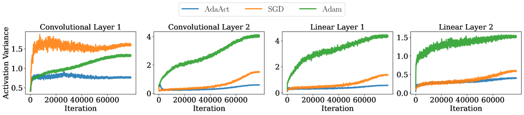
Figure 8: Activation variance resulted from training LeNet-5 on CIFAR10

We trained LeNet-5 on CIFAR10 for 200 epochs to observe the trend of activation variance over iterations. Figure 8 presents the average of the activation variances across all hidden layers in the architecture. We observe that the activations from layers are bounded.

Appendix E Hyperparameters of Opimizers for Training CIFAR datasets

Table 4: Hyperparameter values used in CIFAR datasets training

	$\eta$	Mom.	$\beta_{1}$	$\beta_{2}$	$\beta_{3}$	$\lambda$	$\epsilon$	$\delta$	$T_{cov}$	$T_{inv}$
SGD	0.1	0.9	.	.	.	$5\times 10^{-4}$	.	.	.	.
AdaAct	0.1	.	0.9	0.999	.	$2\times 10^{-3}$	$1\times 10^{-8}$	.	.	.
Adam	0.001	.	0.9	0.999	.	$5\times 10^{-4}$	$1\times 10^{-8}$	.	.	.
AdamW	0.001	.	0.9	0.999	.	$1\times 10^{-2}$	$1\times 10^{-8}$	.	.	.
Adan	0.01	.	0.98	0.92	0.99	$1\times 10^{-2}$	$1\times 10^{-8}$	.	.	.
FOOF	0.05	0.9	.	0.95	.	$5\times 10^{-4}$	.	1	5	50
KFAC	0.05	0.9	.	0.9	.	$5\times 10^{-4}$	.	1, 10	5	50

$\delta$ denotes the damping factor, $T_{cov}$ is the update period for the covariance matrix of activations or pre-activation gradients, and $T_{inv}$ represents the update period for the inverse of the preconditioning matrix used in FOOF and KFAC. For those two optimizers, $\beta_{2}$ indicates the exponential moving average coefficient for the preconditioner.

References

• [1] Ehsan Amid, Rohan Anil, and Manfred K. Warmuth. Locoprop: Enhancing backprop via local loss optimization. In International Conference on Artificial Intelligence and Statistics, 2021.
• [2] Jimmy Ba, Jamie Ryan Kiros, and Geoffrey E. Hinton. Layer normalization. ArXiv, 2016.
• [3] Frederik Benzing. Gradient descent on neurons and its link to approximate second-order optimization. In International Conference on Machine Learning, 2022.
• [4] Jinghui Chen and Quanquan Gu. Closing the generalization gap of adaptive gradient methods in training deep neural networks. In International Joint Conference on Artificial Intelligence, 2018.
• [5] Jinghui Chen, Dongruo Zhou, Yiqi Tang, Ziyan Yang, Yuan Cao, and Quanquan Gu. Closing the generalization gap of adaptive gradient methods in training deep neural networks. In International Joint Conference on Artificial Intelligence, 2020.
• [6] Xiangning Chen, Cho-Jui Hsieh, and Boqing Gong. When vision transformers outperform resnets without pretraining or strong data augmentations. International Conference on Learning Representations, 2022.
• [7] Xiangyi Chen, Sijia Liu, Ruoyu Sun, and Mingyi Hong. On the convergence of a class of adam-type algorithms for non-convex optimization. In International Conference on Learning Representations, 2019.
• [8] Ekin Dogus Cubuk, Barret Zoph, Jonathon Shlens, and Quoc V. Le. Randaugment: Practical automated data augmentation with a reduced search space. IEEE/CVF Conference on Computer Vision and Pattern Recognition Workshops, 2019.
• [9] Jia Deng, Wei Dong, Richard Socher, Li-Jia Li, Kai Li, and Li Fei-Fei. Imagenet: A large-scale hierarchical image database. In IEEE conference on computer vision and pattern recognition, 2009.
• [10] Ruizhou Ding, Ting-Wu Chin, Zeye Dexter Liu, and Diana Marculescu. Regularizing activation distribution for training binarized deep networks. IEEE/CVF Conference on Computer Vision and Pattern Recognition, 2019.
• [11] Alexey Dosovitskiy, Lucas Beyer, Alexander Kolesnikov, Dirk Weissenborn, Xiaohua Zhai, Thomas Unterthiner, Mostafa Dehghani, Matthias Minderer, Georg Heigold, Sylvain Gelly, Jakob Uszkoreit, and Neil Houlsby. An image is worth 16x16 words: Transformers for image recognition at scale. In International Conference on Learning Representations, 2021.
• [12] Timothy Dozat. Incorporating nesterov momentum into adam. ICLR Workshop, 2016.
• [13] John Duchi, Elad Hazan, and Yoram Singer. Adaptive subgradient methods for online learning and stochastic optimization. Journal of Machine Learning Research, 2011.
• [14] Pierre Foret, Ariel Kleiner, Hossein Mobahi, and Behnam Neyshabur. Sharpness-aware minimization for efficiently improving generalization. In International Conference on Learning Representations, 2021.
• [15] Qiang Fu, Lun Du, Haitao Mao, Xu Chen, Wei Fang, Shi Han, and Dongmei Zhang. Neuron with steady response leads to better generalization. In Neural Information Processing Systems, 2022.
• [16] Priya Goyal, Piotr Dollár, Ross B. Girshick, Pieter Noordhuis, Lukasz Wesolowski, Aapo Kyrola, Andrew Tulloch, Yangqing Jia, and Kaiming He. Accurate, large minibatch sgd: Training imagenet in 1 hour. ArXiv, 2017.
• [17] Moritz Hardt, Benjamin Recht, and Yoram Singer. Train faster, generalize better: Stability of stochastic gradient descent. In International Conference on Machine Learning, 2016.
• [18] Kaiming He, Xiangyu Zhang, Shaoqing Ren, and Jian Sun. Deep residual learning for image recognition. In IEEE Conference on Computer Vision and Pattern Recognition, 2016.
• [19] Gao Huang, Zhuang Liu, and Kilian Q. Weinberger. Densely connected convolutional networks. IEEE Conference on Computer Vision and Pattern Recognition, 2016.
• [20] Gao Huang, Yu Sun, Zhuang Liu, Daniel Sedra, and Kilian Q. Weinberger. Deep networks with stochastic depth. In European Conference on Computer Vision, 2016.
• [21] Yasutoshi Ida, Yasuhiro Fujiwara, and Sotetsu Iwamura. Adaptive learning rate via covariance matrix based preconditioning for deep neural networks. In International Joint Conference on Artificial Intelligence, 2016.
• [22] Sergey Ioffe and Christian Szegedy. Batch normalization: Accelerating deep network training by reducing internal covariate shift. In International Conference on Machine Learning, 2015.
• [23] Taejong Joo, Donggu Kang, and Byunghoon Kim. Regularizing activations in neural networks via distribution matching with the wasserstein metric. In International Conference on Learning Representations, 2020.
• [24] Nitish Shirish Keskar and Richard Socher. Improving generalization performance by switching from adam to sgd. arXiv, 2017.
• [25] Diederik P. Kingma and Jimmy Ba. Adam: A method for stochastic optimization. In International Conference on Learning Representations, 2015.
• [26] Alex Krizhevsky. Learning multiple layers of features from tiny images. Technical report, Citeseer, 2009.
• [27] David Krueger and Roland Memisevic. Regularizing rnns by stabilizing activations. In Advances in Neural Information Processing Systems, 2015.
• [28] Y. Lecun, L. Bottou, Y. Bengio, and P. Haffner. Gradient-based learning applied to document recognition. Proceedings of the IEEE, 1998.
• [29] Etai Littwin and Lior Wolf. Regularizing by the variance of the activations’ sample-variances. In Conference on Neural Information Processing Systems, 2018.
• [30] Liyuan Liu, Haoming Jiang, Pengcheng He, Weizhu Chen, Xiaodong Liu, Jianfeng Gao, and Jiawei Han. On the variance of the adaptive learning rate and beyond. In International Conference on Learning Representations, 2020.
• [31] Mingrui Liu, Wei Zhang, Francesco Orabona, and Tianbao Yang. Adam+: A stochastic method with adaptive variance reduction, 2021.
• [32] Ilya Loshchilov and Frank Hutter. Decoupled weight decay regularization. In International Conference on Learning Representations, 2019.
• [33] Liangchen Luo, Yuanhao Xiong, Yan Liu, and Xu Sun. Adaptive gradient methods with dynamic bound of learning rate. In International Conference on Learning Representations, 2019.
• [34] James Martens and Roger Grosse. Optimizing neural networks with kronecker-factored approximate curvature. In International Conference on Machine Learning, 2015.
• [35] Stephen Merity, Bryan McCann, and Richard Socher. Revisiting activation regularization for language rnns. ArXiv, 2017.
• [36] Sashank J. Reddi, Satyen Kale, and Sanjiv Kumar. On the convergence of adam and beyond. In International Conference on Learning Representations, 2019.
• [37] Nitish Srivastava, Geoffrey Hinton, Alex Krizhevsky, Ilya Sutskever, and Ruslan Salakhutdinov. Dropout: A simple way to prevent neural networks from overfitting. Journal of Machine Learning Research, 2014.
• [38] Ilya Sutskever, James Martens, George E. Dahl, and Geoffrey E. Hinton. On the importance of initialization and momentum in deep learning. In International Conference on Machine Learning, 2013.
• [39] T. Tieleman and G. Hinton. Lecture 6.5-rmsprop: Divide the gradient by a running average of its recent magnitude. COURSERA: Neural Networks for Machine Learning, 2012.
• [40] Ashish Vaswani, Noam M. Shazeer, Niki Parmar, Jakob Uszkoreit, Llion Jones, Aidan N. Gomez, Lukasz Kaiser, and Illia Polosukhin. Attention is all you need. In Neural Information Processing Systems, 2017.
• [41] Ross Wightman. Pytorch image models. https://github.com/rwightman/pytorch-image-models, 2019.
• [42] Ross Wightman, Hugo Touvron, and Herve Jegou. Resnet strikes back: An improved training procedure in timm. In NeurIPS 2021 Workshop on ImageNet: Past, Present, and Future, 2021.
• [43] Ashia C. Wilson, Rebecca Roelofs, Mitchell Stern, Nathan Srebro, and Benjamin Recht. The marginal value of adaptive gradient methods in machine learning. In Neural Information Processing Systems, 2017.
• [44] Han Xiao, Kashif Rasul, and Roland Vollgraf. Fashion-mnist: a novel image dataset for benchmarking machine learning algorithms, 2017.
• [45] Xingyu Xie, Pan Zhou, Huan Li, Zhouchen Lin, and Shuicheng YAN. Adan: Adaptive nesterov momentum algorithm for faster optimizing deep models. In Has it Trained Yet? NeurIPS 2022 Workshop, 2022.
• [46] Zeke Xie, Xinrui Wang, Huishuai Zhang, Issei Sato, and Masashi Sugiyama. Adaptive inertia: Disentangling the effects of adaptive learning rate and momentum. In International Conference on Machine Learning, 2020.
• [47] Yang You, Jing Li, Sashank Reddi, Jonathan Hseu, Sanjiv Kumar, Srinadh Bhojanapalli, Xiaodan Song, James Demmel, Kurt Keutzer, and Cho-Jui Hsieh. Large batch optimization for deep learning: Training bert in 76 minutes. In International Conference on Learning Representations, 2020.
• [48] Sangdoo Yun, Dongyoon Han, Seong Joon Oh, Sanghyuk Chun, Junsuk Choe, and Young Joon Yoo. Cutmix: Regularization strategy to train strong classifiers with localizable features. IEEE/CVF International Conference on Computer Vision, 2019.
• [49] Hongyi Zhang, Moustapha Cisse, Yann N. Dauphin, and David Lopez-Paz. mixup: Beyond empirical risk minimization. In International Conference on Learning Representations, 2018.
• [50] Lin Zhang, Shaohuai Shi, and Bo Li. Eva: Practical second-order optimization with kronecker-vectorized approximation. In International Conference on Learning Representations, 2023.
• [51] Juntang Zhuang, Tommy Tang, Yifan Ding, Sekhar C Tatikonda, Nicha Dvornek, Xenophon Papademetris, and James Duncan. Adabelief optimizer: Adapting stepsizes by the belief in observed gradients. Advances in Neural Information Processing Systems, 2020.