Optical theorem and generalized energy conservation for scattering of time-modulated waves

Abstract

We introduce and study a generalized energy conservation relation for scattering of time-modulated waves, where conventional energy conservation does not hold. Based on this relation, we derive an optical theorem and compute the active power describing the power input or output due to scattering. Notably, the same system may be subject to energy gain, energy loss, or energy conservation depending on the frequency harmonics present in the wave field. Moreover, we show how the optical theorem derived herein may be used for image reconstruction based on measurements of the power. Notably, such measurements do not require information about the phase of the scattered field.

I Introduction

The field of Floquet metamaterials, also known as time-modulated materials or spacetime materials, is of considerable recent interest. The underlying physical mechanism is to break time-reversal symmetry, by using a medium with a time-dependent refractive index. Notable phenomena, such as frequency conversion and parametric amplification, arise as a consequence of broken energy conservation [1, 2]. A compelling class of systems feature “travelling-wave”-like modulation, which is a natural setting for non-reciprocal wave propagation, and have recently been shown to satisfy generalized energy conservation relations [3, 4, 5]. Similarly, generalized energy estimates for wave equations with variable wave speeds typically feature terms which grow exponentially, enabling parametric amplification [6, 7, 8, 9, 10, 11]. For scattering from a compactly supported potential, this may be understood as an instability of the system. Scattering resonances, which typically lie in the complex lower half-plane, may cross the real axis and attain a positive imaginary part [12, 13, 2, 14, 15]. The associated quasinormal modes are exponentially growing in time, and the energy input exceeds the radiative losses into the far-field. For nonlinear systems, energy-preserving mechanisms for time-modulated materials have been proposed to overcome such instabilities [16].

An ideal time-dependent material only violates energy conservation when a wave field is present [17]. When illuminated by an incident field, the scattered field is no longer governed by the standard optical theorem, and the material may inject or absorb energy into the scattered field. In this work, we derive a generalized energy conservation law and optical theorem for such scattering systems. We show that the classical energy conservation law must be supplemented with a source term which accounts for the energy balance of the system. Moreover, we demonstrate that the same system may have energy gain, energy loss, or energy conservation, depending on the wave harmonics present in the incident field. This may be understood as an energy imbalance due to frequency conversion, and a conserved quantity arises by redefining the weights of the energy current associated to each frequency harmonic. Notably, we consider stable systems. The energy gain we observe is not due to parametric amplification, and the resulting field does not grow exponentially at large times.

We demonstrate the applicability of our optical theorem for imaging of time-modulated systems, without the need to measure the phase of the field. Reconstruction without phase retrieval, based on generalizations of the optical theorem, has been studied for near-field imaging of static systems [18, 19, 20]. In the weak-scattering regime, it is only possible to reconstruct the absorption of the material coefficients of static systems. In contrast, the broken energy conservation of time-modulated systems enables reconstruction of the time-dependent material coefficients. However, the discrepancy between the probing frequency and the measured frequency (caused by frequency conversion) introduces a lower band-limit in addition to the usual upper band limit. The upper band limit behaves analogously to the diffraction limit and restricts the image reconstruction to short length scales. In contrast, the lower band limit causes spatial characteristics of long length scales to be unresolvable.

This paper is organized as follows. In Section II, we consider energy conservation of the homogeneous wave equation. The setting is standard, and these results are foundational for the remainder of the work. In Section III, we show how the time-modulated model we consider can be derived from first principles. In Section IV, we derive a generalized energy conservation law for this model, containing a source term which accounts for energy gain or absorption. In Section V, we formulate the optical theorem for time-modulated systems and present a detailed analysis of the energy balance of point scatterers. In Section VI, we consider the weak-scattering approximation, and show how the optical theorem can be used as basis for image reconstruction based on measurements of the wave power. We end the paper with some concluding remarks in Section VII.

II Energy density conservation for the scalar wave equation

We begin by summarizing a few results, which will be used later on, concerning the scalar wave equation in the absence of time-dependent scatterers. This setting is standard, and may be found in, e.g., [21, 22]. For $\mathbf{x}\in\mathbb{R}^{3}$ and $t\in\mathbb{R}$, we consider the wave equation with wave speed $c_{0}$,

$$\frac{\partial^{2}}{\partial t^{2}}u(\mathbf{x},t)-c_{0}^{2}\Delta u(\mathbf{x},t)=0.$$ (1)

We let the energy density $E(\mathbf{x},t)$ be defined as

$$E(\mathbf{x},t)=\frac{1}{2}\left(\frac{1}{c_{0}^{2}}\left|\frac{\partial u}{\partial t}\right|^{2}+\left|\nabla u\right|^{2}\right).$$ (2)

This energy density is associated to the energy density current $\mathbf{S}(\mathbf{x},t)$ given by

$$\mathbf{S}(\mathbf{x},t)=-\mathrm{Re}\left(\frac{\partial\overline{u}}{\partial t}\nabla u\right).$$ (3)

Here, and throughout, we use superscript $\overline{\phantom{a}}$ to denote complex conjugate, and ^∗ to denote the transpose conjugate of a matrix. $E$ and $\mathbf{S}$ obey the classical energy conservation law

$$\frac{\partial E}{\partial t}=-\nabla\cdot\mathbf{S}.$$ (4)

If we consider a wave composed of multiple frequency harmonics centered at some quasifrequency $\omega\in\mathbb{R}$, i.e.,

$$u(\mathbf{x},t)=\sum_{m=-\infty}^{\infty}v_{m}(\mathbf{x})e^{-\mathrm{i}\mkern 1.0mu(\omega+m\Omega)t},$$ (5)

we may pose the conservation law in the frequency domain. By time-averaging $\mathbf{S}$ over one period $T=\frac{2\pi}{\Omega}$, we obtain

$$\langle\mathbf{S}(\mathbf{x},t)\rangle=c_{0}\sum_{m=-\infty}^{\infty}\mathbf{J}_{m}(\mathbf{x})$$ (6)

where

$$\mathbf{J}_{m}=\frac{k_{n}}{2\mathrm{i}\mkern 1.0mu}\left(\overline{v_{m}}\nabla v_{m}-v_{m}\nabla\overline{v_{m}}\right),\qquad\mathbf{J}=\sum_{m=-\infty}^{\infty}\mathbf{J}_{m},$$ (7)

and where we have defined $k_{m}=\frac{\omega+m\Omega}{c_{0}}$. In the frequency domain, we then have the conservation law

$$\nabla\cdot\mathbf{J}=0.$$ (8)

III Time-modulated acoustic wave equation

We now define the time-modulated model which will be studied in the remainder of this work. We consider the acoustic wave equation with time-varying wave speed $c$ which has appeared, for example, in [23]. To define the model, we start with the linearized Euler equation and mass conservation,

$$\begin{cases}\displaystyle\rho_{0}\frac{\partial\mathbf{v}}{\partial t}=-\nabla p_{1},\\ \displaystyle\frac{\partial\rho_{1}}{\partial t}+\rho_{0}\nabla\cdot\mathbf{v}=0.\end{cases}$$ (9)

Here, $\mathbf{v}$ is the velocity field of the acoustic medium, $\rho_{0}$ is the equilibrium density while $p_{1}$ and $\rho_{1}$, respectively, are the pressure and density fluctuations due to the acoustic wave. Moreover, we consider the linearized equation of state

$$p_{1}(\mathbf{x},t)=c^{2}\rho_{1}(\mathbf{x},t).$$ (10)

Here, $c$ is the speed of acoustic waves. We consider a situation whereby $c=c(\mathbf{x},t)$ is periodically modulated in time. To preserve mass balance, we take a constant $\rho_{0}$. In this case, we obtain the time-modulated wave equation

$$\frac{\partial^{2}}{\partial t^{2}}\left(\frac{1}{c^{2}(\mathbf{x},t)}p_{1}(\mathbf{x},t)\right)-\Delta p_{1}(\mathbf{x},t)=0.$$ (11)

Equation (11) describes scalar waves with a time-modulated refractive index: For a reference wave speed $c_{0}$ (constant in $t$ and $\mathbf{x}$) we let the refractive index $n(\mathbf{x},t)$ be defined through

$$c(\mathbf{x},t)=\frac{c_{0}}{n(\mathbf{x},t)}.$$ (12)

IV Generalized energy conservation

We now turn to the problem with time-dependent scatterers and derive a generalized energy conservation. We consider the equation

$$\frac{\partial^{2}}{\partial t^{2}}\left(\frac{n^{2}(\mathbf{x},t)}{c_{0}^{2}}u(\mathbf{x},t)\right)-\Delta u(\mathbf{x},t)=0,\quad\mathbf{x}\in\mathbb{R}^{3},t\in\mathbb{R},$$ (13)

where $n(\mathbf{x},t)$ is $T$-periodic in $t$. By Bloch’s theorem in $t$, we seek solutions which are quasiperiodic in $t$:

$$u(\mathbf{x},t)=\sum_{m=-\infty}^{\infty}v_{m}(\mathbf{x})e^{-\mathrm{i}\mkern 1.0mu(\omega+m\Omega)t},$$ (14)

where $\Omega=\frac{2\pi}{T}$. We let $\eta$ be the perturbation of $n^{2}$ against a (constant) background:

$$n^{2}(\mathbf{x},t)=1+\eta(\mathbf{x},t).$$ (15)

We consider a general (possibly complex-valued) spacetime-varying $\eta(\mathbf{x},t)$ with Fourier coefficients $\eta_{m}(\mathbf{x})$, i.e.,

$$\eta(\mathbf{x},t)=\sum_{m=-\infty}^{\infty}\eta_{m}(\mathbf{x})e^{-\mathrm{i}\mkern 1.0mum\Omega t}.$$ (16)

Substituting into (13) results in a system of coupled equations

$$\begin{split}&\Delta v_{m}+k_{m}^{2}v_{m}+k_{m}^{2}\sum_{l=-\infty}^{\infty}\eta_{m-l}(\mathbf{x})v_{l}=0,\end{split}$$ (17)

where, as before, $\frac{\omega+m\Omega}{c_{0}}$. We begin by writing (17) in matrix form: define the (doubly infinite) Toeplitz matrix $H=H(\mathbf{x})$ and the diagonal matrix $K$ as

$$H=\begin{pmatrix}\mathinner{\mathchoice{\vbox{\kern 3.23996pt\vbox to7.43826pt{\offinterlineskip\hbox{$\displaystyle\mathpunct{.}$}\vfill\hbox{$\displaystyle\mathpunct{\kern 2.2639pt}\mathpunct{.}$}\vfill\hbox{$\displaystyle\mathpunct{\kern 2.2639pt}\mathpunct{\kern 2.2639pt}\mathpunct{.}$}}}}{\vbox{\kern 3.23996pt\vbox to7.43826pt{\offinterlineskip\hbox{$\textstyle\mathpunct{.}$}\vfill\hbox{$\textstyle\mathpunct{\kern 2.2639pt}\mathpunct{.}$}\vfill\hbox{$\textstyle\mathpunct{\kern 2.2639pt}\mathpunct{\kern 2.2639pt}\mathpunct{.}$}}}}{\vbox{\kern 2.15166pt\vbox to5.01105pt{\offinterlineskip\hbox{$\scriptstyle\mathpunct{.}$}\vfill\hbox{$\scriptstyle\mathpunct{\kern 1.36111pt}\mathpunct{.}$}\vfill\hbox{$\scriptstyle\mathpunct{\kern 1.36111pt}\mathpunct{\kern 1.36111pt}\mathpunct{.}$}}}}{\vbox{\kern 1.78998pt\vbox to4.08546pt{\offinterlineskip\hbox{$\scriptscriptstyle\mathpunct{.}$}\vfill\hbox{$\scriptscriptstyle\mathpunct{\kern 0.97221pt}\mathpunct{.}$}\vfill\hbox{$\scriptscriptstyle\mathpunct{\kern 0.97221pt}\mathpunct{\kern 0.97221pt}\mathpunct{.}$}}}}\mkern 3.0mu}&\mathinner{\mathchoice{\vbox{\kern 3.23996pt\vbox to7.43826pt{\offinterlineskip\hbox{$\displaystyle\mathpunct{.}$}\vfill\hbox{$\displaystyle\mathpunct{\kern 2.2639pt}\mathpunct{.}$}\vfill\hbox{$\displaystyle\mathpunct{\kern 2.2639pt}\mathpunct{\kern 2.2639pt}\mathpunct{.}$}}}}{\vbox{\kern 3.23996pt\vbox to7.43826pt{\offinterlineskip\hbox{$\textstyle\mathpunct{.}$}\vfill\hbox{$\textstyle\mathpunct{\kern 2.2639pt}\mathpunct{.}$}\vfill\hbox{$\textstyle\mathpunct{\kern 2.2639pt}\mathpunct{\kern 2.2639pt}\mathpunct{.}$}}}}{\vbox{\kern 2.15166pt\vbox to5.01105pt{\offinterlineskip\hbox{$\scriptstyle\mathpunct{.}$}\vfill\hbox{$\scriptstyle\mathpunct{\kern 1.36111pt}\mathpunct{.}$}\vfill\hbox{$\scriptstyle\mathpunct{\kern 1.36111pt}\mathpunct{\kern 1.36111pt}\mathpunct{.}$}}}}{\vbox{\kern 1.78998pt\vbox to4.08546pt{\offinterlineskip\hbox{$\scriptscriptstyle\mathpunct{.}$}\vfill\hbox{$\scriptscriptstyle\mathpunct{\kern 0.97221pt}\mathpunct{.}$}\vfill\hbox{$\scriptscriptstyle\mathpunct{\kern 0.97221pt}\mathpunct{\kern 0.97221pt}\mathpunct{.}$}}}}\mkern 3.0mu}&\mathinner{\mathchoice{\vbox{\kern 3.23996pt\vbox to7.43826pt{\offinterlineskip\hbox{$\displaystyle\mathpunct{.}$}\vfill\hbox{$\displaystyle\mathpunct{\kern 2.2639pt}\mathpunct{.}$}\vfill\hbox{$\displaystyle\mathpunct{\kern 2.2639pt}\mathpunct{\kern 2.2639pt}\mathpunct{.}$}}}}{\vbox{\kern 3.23996pt\vbox to7.43826pt{\offinterlineskip\hbox{$\textstyle\mathpunct{.}$}\vfill\hbox{$\textstyle\mathpunct{\kern 2.2639pt}\mathpunct{.}$}\vfill\hbox{$\textstyle\mathpunct{\kern 2.2639pt}\mathpunct{\kern 2.2639pt}\mathpunct{.}$}}}}{\vbox{\kern 2.15166pt\vbox to5.01105pt{\offinterlineskip\hbox{$\scriptstyle\mathpunct{.}$}\vfill\hbox{$\scriptstyle\mathpunct{\kern 1.36111pt}\mathpunct{.}$}\vfill\hbox{$\scriptstyle\mathpunct{\kern 1.36111pt}\mathpunct{\kern 1.36111pt}\mathpunct{.}$}}}}{\vbox{\kern 1.78998pt\vbox to4.08546pt{\offinterlineskip\hbox{$\scriptscriptstyle\mathpunct{.}$}\vfill\hbox{$\scriptscriptstyle\mathpunct{\kern 0.97221pt}\mathpunct{.}$}\vfill\hbox{$\scriptscriptstyle\mathpunct{\kern 0.97221pt}\mathpunct{\kern 0.97221pt}\mathpunct{.}$}}}}\mkern 3.0mu}&&\hskip-5.0pt\\ \mathinner{\mathchoice{\vbox{\kern 3.23996pt\vbox to7.43826pt{\offinterlineskip\hbox{$\displaystyle\mathpunct{.}$}\vfill\hbox{$\displaystyle\mathpunct{\kern 2.2639pt}\mathpunct{.}$}\vfill\hbox{$\displaystyle\mathpunct{\kern 2.2639pt}\mathpunct{\kern 2.2639pt}\mathpunct{.}$}}}}{\vbox{\kern 3.23996pt\vbox to7.43826pt{\offinterlineskip\hbox{$\textstyle\mathpunct{.}$}\vfill\hbox{$\textstyle\mathpunct{\kern 2.2639pt}\mathpunct{.}$}\vfill\hbox{$\textstyle\mathpunct{\kern 2.2639pt}\mathpunct{\kern 2.2639pt}\mathpunct{.}$}}}}{\vbox{\kern 2.15166pt\vbox to5.01105pt{\offinterlineskip\hbox{$\scriptstyle\mathpunct{.}$}\vfill\hbox{$\scriptstyle\mathpunct{\kern 1.36111pt}\mathpunct{.}$}\vfill\hbox{$\scriptstyle\mathpunct{\kern 1.36111pt}\mathpunct{\kern 1.36111pt}\mathpunct{.}$}}}}{\vbox{\kern 1.78998pt\vbox to4.08546pt{\offinterlineskip\hbox{$\scriptscriptstyle\mathpunct{.}$}\vfill\hbox{$\scriptscriptstyle\mathpunct{\kern 0.97221pt}\mathpunct{.}$}\vfill\hbox{$\scriptscriptstyle\mathpunct{\kern 0.97221pt}\mathpunct{\kern 0.97221pt}\mathpunct{.}$}}}}\mkern 3.0mu}&\eta_{0}&\eta_{-1}&\eta_{-2}&\\ \mathinner{\mathchoice{\vbox{\kern 3.23996pt\vbox to7.43826pt{\offinterlineskip\hbox{$\displaystyle\mathpunct{.}$}\vfill\hbox{$\displaystyle\mathpunct{\kern 2.2639pt}\mathpunct{.}$}\vfill\hbox{$\displaystyle\mathpunct{\kern 2.2639pt}\mathpunct{\kern 2.2639pt}\mathpunct{.}$}}}}{\vbox{\kern 3.23996pt\vbox to7.43826pt{\offinterlineskip\hbox{$\textstyle\mathpunct{.}$}\vfill\hbox{$\textstyle\mathpunct{\kern 2.2639pt}\mathpunct{.}$}\vfill\hbox{$\textstyle\mathpunct{\kern 2.2639pt}\mathpunct{\kern 2.2639pt}\mathpunct{.}$}}}}{\vbox{\kern 2.15166pt\vbox to5.01105pt{\offinterlineskip\hbox{$\scriptstyle\mathpunct{.}$}\vfill\hbox{$\scriptstyle\mathpunct{\kern 1.36111pt}\mathpunct{.}$}\vfill\hbox{$\scriptstyle\mathpunct{\kern 1.36111pt}\mathpunct{\kern 1.36111pt}\mathpunct{.}$}}}}{\vbox{\kern 1.78998pt\vbox to4.08546pt{\offinterlineskip\hbox{$\scriptscriptstyle\mathpunct{.}$}\vfill\hbox{$\scriptscriptstyle\mathpunct{\kern 0.97221pt}\mathpunct{.}$}\vfill\hbox{$\scriptscriptstyle\mathpunct{\kern 0.97221pt}\mathpunct{\kern 0.97221pt}\mathpunct{.}$}}}}\mkern 3.0mu}&\eta_{1}&\eta_{0}&\eta_{-1}&\mathinner{\mathchoice{\vbox{\kern 3.23996pt\vbox to7.43826pt{\offinterlineskip\hbox{$\displaystyle\mathpunct{.}$}\vfill\hbox{$\displaystyle\mathpunct{\kern 2.2639pt}\mathpunct{.}$}\vfill\hbox{$\displaystyle\mathpunct{\kern 2.2639pt}\mathpunct{\kern 2.2639pt}\mathpunct{.}$}}}}{\vbox{\kern 3.23996pt\vbox to7.43826pt{\offinterlineskip\hbox{$\textstyle\mathpunct{.}$}\vfill\hbox{$\textstyle\mathpunct{\kern 2.2639pt}\mathpunct{.}$}\vfill\hbox{$\textstyle\mathpunct{\kern 2.2639pt}\mathpunct{\kern 2.2639pt}\mathpunct{.}$}}}}{\vbox{\kern 2.15166pt\vbox to5.01105pt{\offinterlineskip\hbox{$\scriptstyle\mathpunct{.}$}\vfill\hbox{$\scriptstyle\mathpunct{\kern 1.36111pt}\mathpunct{.}$}\vfill\hbox{$\scriptstyle\mathpunct{\kern 1.36111pt}\mathpunct{\kern 1.36111pt}\mathpunct{.}$}}}}{\vbox{\kern 1.78998pt\vbox to4.08546pt{\offinterlineskip\hbox{$\scriptscriptstyle\mathpunct{.}$}\vfill\hbox{$\scriptscriptstyle\mathpunct{\kern 0.97221pt}\mathpunct{.}$}\vfill\hbox{$\scriptscriptstyle\mathpunct{\kern 0.97221pt}\mathpunct{\kern 0.97221pt}\mathpunct{.}$}}}}\mkern 3.0mu}\\ &\eta_{2}&\eta_{1}&\eta_{0}&\mathinner{\mathchoice{\vbox{\kern 3.23996pt\vbox to7.43826pt{\offinterlineskip\hbox{$\displaystyle\mathpunct{.}$}\vfill\hbox{$\displaystyle\mathpunct{\kern 2.2639pt}\mathpunct{.}$}\vfill\hbox{$\displaystyle\mathpunct{\kern 2.2639pt}\mathpunct{\kern 2.2639pt}\mathpunct{.}$}}}}{\vbox{\kern 3.23996pt\vbox to7.43826pt{\offinterlineskip\hbox{$\textstyle\mathpunct{.}$}\vfill\hbox{$\textstyle\mathpunct{\kern 2.2639pt}\mathpunct{.}$}\vfill\hbox{$\textstyle\mathpunct{\kern 2.2639pt}\mathpunct{\kern 2.2639pt}\mathpunct{.}$}}}}{\vbox{\kern 2.15166pt\vbox to5.01105pt{\offinterlineskip\hbox{$\scriptstyle\mathpunct{.}$}\vfill\hbox{$\scriptstyle\mathpunct{\kern 1.36111pt}\mathpunct{.}$}\vfill\hbox{$\scriptstyle\mathpunct{\kern 1.36111pt}\mathpunct{\kern 1.36111pt}\mathpunct{.}$}}}}{\vbox{\kern 1.78998pt\vbox to4.08546pt{\offinterlineskip\hbox{$\scriptscriptstyle\mathpunct{.}$}\vfill\hbox{$\scriptscriptstyle\mathpunct{\kern 0.97221pt}\mathpunct{.}$}\vfill\hbox{$\scriptscriptstyle\mathpunct{\kern 0.97221pt}\mathpunct{\kern 0.97221pt}\mathpunct{.}$}}}}\mkern 3.0mu}\\ &&\mathinner{\mathchoice{\vbox{\kern 3.23996pt\vbox to7.43826pt{\offinterlineskip\hbox{$\displaystyle\mathpunct{.}$}\vfill\hbox{$\displaystyle\mathpunct{\kern 2.2639pt}\mathpunct{.}$}\vfill\hbox{$\displaystyle\mathpunct{\kern 2.2639pt}\mathpunct{\kern 2.2639pt}\mathpunct{.}$}}}}{\vbox{\kern 3.23996pt\vbox to7.43826pt{\offinterlineskip\hbox{$\textstyle\mathpunct{.}$}\vfill\hbox{$\textstyle\mathpunct{\kern 2.2639pt}\mathpunct{.}$}\vfill\hbox{$\textstyle\mathpunct{\kern 2.2639pt}\mathpunct{\kern 2.2639pt}\mathpunct{.}$}}}}{\vbox{\kern 2.15166pt\vbox to5.01105pt{\offinterlineskip\hbox{$\scriptstyle\mathpunct{.}$}\vfill\hbox{$\scriptstyle\mathpunct{\kern 1.36111pt}\mathpunct{.}$}\vfill\hbox{$\scriptstyle\mathpunct{\kern 1.36111pt}\mathpunct{\kern 1.36111pt}\mathpunct{.}$}}}}{\vbox{\kern 1.78998pt\vbox to4.08546pt{\offinterlineskip\hbox{$\scriptscriptstyle\mathpunct{.}$}\vfill\hbox{$\scriptscriptstyle\mathpunct{\kern 0.97221pt}\mathpunct{.}$}\vfill\hbox{$\scriptscriptstyle\mathpunct{\kern 0.97221pt}\mathpunct{\kern 0.97221pt}\mathpunct{.}$}}}}\mkern 3.0mu}&\mathinner{\mathchoice{\vbox{\kern 3.23996pt\vbox to7.43826pt{\offinterlineskip\hbox{$\displaystyle\mathpunct{.}$}\vfill\hbox{$\displaystyle\mathpunct{\kern 2.2639pt}\mathpunct{.}$}\vfill\hbox{$\displaystyle\mathpunct{\kern 2.2639pt}\mathpunct{\kern 2.2639pt}\mathpunct{.}$}}}}{\vbox{\kern 3.23996pt\vbox to7.43826pt{\offinterlineskip\hbox{$\textstyle\mathpunct{.}$}\vfill\hbox{$\textstyle\mathpunct{\kern 2.2639pt}\mathpunct{.}$}\vfill\hbox{$\textstyle\mathpunct{\kern 2.2639pt}\mathpunct{\kern 2.2639pt}\mathpunct{.}$}}}}{\vbox{\kern 2.15166pt\vbox to5.01105pt{\offinterlineskip\hbox{$\scriptstyle\mathpunct{.}$}\vfill\hbox{$\scriptstyle\mathpunct{\kern 1.36111pt}\mathpunct{.}$}\vfill\hbox{$\scriptstyle\mathpunct{\kern 1.36111pt}\mathpunct{\kern 1.36111pt}\mathpunct{.}$}}}}{\vbox{\kern 1.78998pt\vbox to4.08546pt{\offinterlineskip\hbox{$\scriptscriptstyle\mathpunct{.}$}\vfill\hbox{$\scriptscriptstyle\mathpunct{\kern 0.97221pt}\mathpunct{.}$}\vfill\hbox{$\scriptscriptstyle\mathpunct{\kern 0.97221pt}\mathpunct{\kern 0.97221pt}\mathpunct{.}$}}}}\mkern 3.0mu}&\mathinner{\mathchoice{\vbox{\kern 3.23996pt\vbox to7.43826pt{\offinterlineskip\hbox{$\displaystyle\mathpunct{.}$}\vfill\hbox{$\displaystyle\mathpunct{\kern 2.2639pt}\mathpunct{.}$}\vfill\hbox{$\displaystyle\mathpunct{\kern 2.2639pt}\mathpunct{\kern 2.2639pt}\mathpunct{.}$}}}}{\vbox{\kern 3.23996pt\vbox to7.43826pt{\offinterlineskip\hbox{$\textstyle\mathpunct{.}$}\vfill\hbox{$\textstyle\mathpunct{\kern 2.2639pt}\mathpunct{.}$}\vfill\hbox{$\textstyle\mathpunct{\kern 2.2639pt}\mathpunct{\kern 2.2639pt}\mathpunct{.}$}}}}{\vbox{\kern 2.15166pt\vbox to5.01105pt{\offinterlineskip\hbox{$\scriptstyle\mathpunct{.}$}\vfill\hbox{$\scriptstyle\mathpunct{\kern 1.36111pt}\mathpunct{.}$}\vfill\hbox{$\scriptstyle\mathpunct{\kern 1.36111pt}\mathpunct{\kern 1.36111pt}\mathpunct{.}$}}}}{\vbox{\kern 1.78998pt\vbox to4.08546pt{\offinterlineskip\hbox{$\scriptscriptstyle\mathpunct{.}$}\vfill\hbox{$\scriptscriptstyle\mathpunct{\kern 0.97221pt}\mathpunct{.}$}\vfill\hbox{$\scriptscriptstyle\mathpunct{\kern 0.97221pt}\mathpunct{\kern 0.97221pt}\mathpunct{.}$}}}}\mkern 3.0mu}\end{pmatrix},\quad K=\begin{pmatrix}\mathinner{\mathchoice{\vbox{\kern 3.23996pt\vbox to7.43826pt{\offinterlineskip\hbox{$\displaystyle\mathpunct{.}$}\vfill\hbox{$\displaystyle\mathpunct{\kern 2.2639pt}\mathpunct{.}$}\vfill\hbox{$\displaystyle\mathpunct{\kern 2.2639pt}\mathpunct{\kern 2.2639pt}\mathpunct{.}$}}}}{\vbox{\kern 3.23996pt\vbox to7.43826pt{\offinterlineskip\hbox{$\textstyle\mathpunct{.}$}\vfill\hbox{$\textstyle\mathpunct{\kern 2.2639pt}\mathpunct{.}$}\vfill\hbox{$\textstyle\mathpunct{\kern 2.2639pt}\mathpunct{\kern 2.2639pt}\mathpunct{.}$}}}}{\vbox{\kern 2.15166pt\vbox to5.01105pt{\offinterlineskip\hbox{$\scriptstyle\mathpunct{.}$}\vfill\hbox{$\scriptstyle\mathpunct{\kern 1.36111pt}\mathpunct{.}$}\vfill\hbox{$\scriptstyle\mathpunct{\kern 1.36111pt}\mathpunct{\kern 1.36111pt}\mathpunct{.}$}}}}{\vbox{\kern 1.78998pt\vbox to4.08546pt{\offinterlineskip\hbox{$\scriptscriptstyle\mathpunct{.}$}\vfill\hbox{$\scriptscriptstyle\mathpunct{\kern 0.97221pt}\mathpunct{.}$}\vfill\hbox{$\scriptscriptstyle\mathpunct{\kern 0.97221pt}\mathpunct{\kern 0.97221pt}\mathpunct{.}$}}}}\mkern 3.0mu}\hskip-3.0pt&&&&\\ &k_{-1}\hskip-5.0pt&&&\\ &&k_{0}\hskip-2.0pt&&\\ &&&k_{1}&\\[-3.00003pt] &&&&\hskip-3.0pt\mathinner{\mathchoice{\vbox{\kern 3.23996pt\vbox to7.43826pt{\offinterlineskip\hbox{$\displaystyle\mathpunct{.}$}\vfill\hbox{$\displaystyle\mathpunct{\kern 2.2639pt}\mathpunct{.}$}\vfill\hbox{$\displaystyle\mathpunct{\kern 2.2639pt}\mathpunct{\kern 2.2639pt}\mathpunct{.}$}}}}{\vbox{\kern 3.23996pt\vbox to7.43826pt{\offinterlineskip\hbox{$\textstyle\mathpunct{.}$}\vfill\hbox{$\textstyle\mathpunct{\kern 2.2639pt}\mathpunct{.}$}\vfill\hbox{$\textstyle\mathpunct{\kern 2.2639pt}\mathpunct{\kern 2.2639pt}\mathpunct{.}$}}}}{\vbox{\kern 2.15166pt\vbox to5.01105pt{\offinterlineskip\hbox{$\scriptstyle\mathpunct{.}$}\vfill\hbox{$\scriptstyle\mathpunct{\kern 1.36111pt}\mathpunct{.}$}\vfill\hbox{$\scriptstyle\mathpunct{\kern 1.36111pt}\mathpunct{\kern 1.36111pt}\mathpunct{.}$}}}}{\vbox{\kern 1.78998pt\vbox to4.08546pt{\offinterlineskip\hbox{$\scriptscriptstyle\mathpunct{.}$}\vfill\hbox{$\scriptscriptstyle\mathpunct{\kern 0.97221pt}\mathpunct{.}$}\vfill\hbox{$\scriptscriptstyle\mathpunct{\kern 0.97221pt}\mathpunct{\kern 0.97221pt}\mathpunct{.}$}}}}\mkern 3.0mu}\end{pmatrix}.$$ (18)

Moreover, let $v(\mathbf{x})=\begin{pmatrix}\mathchoice{\vbox{\kern 3.23996pt\vbox to7.43826pt{\offinterlineskip\hbox{\set@color$\displaystyle.$}\vfill\hbox{\set@color$\displaystyle.$}\vfill\hbox{\set@color$\displaystyle.$}}}}{\vbox{\kern 3.23996pt\vbox to7.43826pt{\offinterlineskip\hbox{\set@color$\textstyle.$}\vfill\hbox{\set@color$\textstyle.$}\vfill\hbox{\set@color$\textstyle.$}}}}{\vbox{\kern 2.15166pt\vbox to5.01105pt{\offinterlineskip\hbox{\set@color$\scriptstyle.$}\vfill\hbox{\set@color$\scriptstyle.$}\vfill\hbox{\set@color$\scriptstyle.$}}}}{\vbox{\kern 1.78998pt\vbox to4.08546pt{\offinterlineskip\hbox{\set@color$\scriptscriptstyle.$}\vfill\hbox{\set@color$\scriptscriptstyle.$}\vfill\hbox{\set@color$\scriptscriptstyle.$}}}}\\[-1.00006pt] v_{-1}\\ v_{0}\\ v_{1}\\[-1.99997pt] \mathchoice{\vbox{\kern 3.23996pt\vbox to7.43826pt{\offinterlineskip\hbox{\set@color$\displaystyle.$}\vfill\hbox{\set@color$\displaystyle.$}\vfill\hbox{\set@color$\displaystyle.$}}}}{\vbox{\kern 3.23996pt\vbox to7.43826pt{\offinterlineskip\hbox{\set@color$\textstyle.$}\vfill\hbox{\set@color$\textstyle.$}\vfill\hbox{\set@color$\textstyle.$}}}}{\vbox{\kern 2.15166pt\vbox to5.01105pt{\offinterlineskip\hbox{\set@color$\scriptstyle.$}\vfill\hbox{\set@color$\scriptstyle.$}\vfill\hbox{\set@color$\scriptstyle.$}}}}{\vbox{\kern 1.78998pt\vbox to4.08546pt{\offinterlineskip\hbox{\set@color$\scriptscriptstyle.$}\vfill\hbox{\set@color$\scriptscriptstyle.$}\vfill\hbox{\set@color$\scriptscriptstyle.$}}}}\end{pmatrix}$. We can then write (17) as

$$\Delta v(\mathbf{x})+K^{2}v(\mathbf{x})+K^{2}H(\mathbf{x})v(\mathbf{x})=0.$$ (19)

We next phrase the conservation law of the energy density current (7) when applied to the spacetime-varying material defined by $\eta(\mathbf{x},t)$. We let $\langle\cdot,\cdot\rangle$ denote the $\ell^{2}$-inner product in the frequency variable. Taking the inner product of (19) by $Kv$ gives

$$\langle Kv,\Delta v\rangle+\langle Kv,K^{2}v\rangle+\langle Kv,K^{2}Hv\rangle=0.$$ (20)

Subtracting by its conjugate (and using the observation that the second term is real), we find

$$\langle Kv,\Delta v\rangle-\langle K\overline{v},\Delta\overline{v}\rangle+\langle Kv,K^{2}Hv\rangle-\langle K\overline{v},K^{2}\overline{H}\overline{v}\rangle=0.$$ (21)

Using the identity $\overline{f}\Delta f-f\Delta\overline{f}=\nabla\cdot\left(\overline{f}\nabla f-f\nabla\overline{f}\right)$, we find that

$$\frac{1}{2\mathrm{i}\mkern 1.0mu}\bigl{(}\langle Kv,\Delta v\rangle-\langle K\overline{v},\Delta\overline{v}\rangle\bigr{)}=\nabla\cdot\sum_{i=-\infty}^{\infty}\mathbf{J}_{i},$$ (22)

where the energy current $\mathbf{J}_{i}$ of the $i$^th harmonic $v_{i}$ is defined as in (7). We also observe that

$$\frac{1}{2\mathrm{i}\mkern 1.0mu}\left(\langle Kv,K^{2}Hv\rangle-\langle K\overline{v},K^{2}\overline{H}\overline{v}\rangle\right)=\langle v,Mv\rangle,$$ (23)

where the matrix $M$ is defined as $M=\frac{1}{2\mathrm{i}\mkern 1.0mu}\left(K^{3}H-\left(K^{3}H\right)^{*}\right)$. Together with (22), we find the conservation law

$$\nabla\cdot\mathbf{J}+\langle v,Mv\rangle=0.$$ (24)

Eq. (24) is the generalized energy conservation of the time-modulated system, and generalizes (8). Note that we do not need to assume that $\eta(\mathbf{x},t)$ is compactly supported in $\mathbf{x}$ for (24) to hold, although this will be the main case considered subsequently.

Observe that, even in the case when $\eta(\mathbf{x},t)$ is real-valued (whereby $H$ is self-adjoint), the matrix $K^{3}H$ is in general not self-adjoint, and $M$ defines a source term for the conservation law. If $\eta(\mathbf{x},t)$ is real-valued and constant in $t$, (24) reduces to the energy conservation $\nabla\cdot\mathbf{J}=0$ for static materials. We can phrase this conservation law in the time domain:

$$\frac{\partial E}{\partial t}=-\nabla\cdot\mathbf{S}-\frac{1}{2c_{0}^{2}}\mathrm{Re}\left(\eta\frac{\partial\overline{u}}{\partial t}\frac{\partial^{2}u}{\partial t^{2}}\right),$$ (25)

which generalizes (4). Here, the source term $\mathrm{Re}\left(\eta\frac{\partial\overline{u}}{\partial t}\frac{\partial^{2}u}{\partial t^{2}}\right)$ corresponds to the operator $M$ in frequency domain.

We note that (24) is phrased for the conventional energy current $\mathbf{J}_{i}$ defined as in (7). For nonabsorbing media, the source term can be eliminated by redefining the weights of the energy current of each frequency harmonic. We define the generalized energy current $\bm{\mathcal{J}}_{i}$ as

$$\bm{\mathcal{J}}_{i}=\frac{1}{2\mathrm{i}\mkern 1.0muk_{i}^{2}}\left(\overline{v_{i}}\nabla v_{i}-v_{i}\nabla\overline{v_{i}}\right).$$ (26)

The conservation law is now given by

$$\nabla\cdot\bm{\mathcal{J}}+\langle v,\mathcal{M}v\rangle=0,$$ (27)

for $\mathcal{M}=\frac{1}{2\mathrm{i}\mkern 1.0mu}\left(H-H^{*}\right).$ In particular, for real-valued $\eta(\mathbf{x},t)$ we have $\mathcal{M}=0$ and $\nabla\cdot\bm{\mathcal{J}}=0$.

V Optical theorem

We now turn to scattering from compactly supported $\eta(\mathbf{x},t)$. When formulating the optical theorem for scattering from a compactly supported time-dependent domain we will consider the conventional current $\mathbf{J}$ defined as in (7); the active energy input/output will be determined through an energy balance in the exterior of the scattering domain. We illustrate the setup and main notation in Fig. 1.

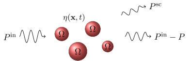
Figure 1: Schematic illustration of the scattering experiment. An incident field to a time-modulated system gives rise to a scattered field of power $P^{\textrm{sc}}$. In the case of energy conservation, $P^{\textrm{sc}}$ must agree with the extinguished power $P$ which is depleted from the incident field. Energy gain corresponds to the case $P^{\textrm{sc}}>P$ while energy absorption corresponds to $P^{\textrm{sc}}<P$.

V.1 Computation of the active and total power

As before, we define the total energy current $\mathbf{J}$ as

$$\mathbf{J}=\sum_{i=-\infty}^{\infty}\frac{k_{i}}{2\mathrm{i}\mkern 1.0mu}\left(\overline{v_{i}}\nabla v_{i}-v_{i}\nabla\overline{v_{i}}\right).$$ (28)

We separate the field $v_{i}$ into incident and scattered fields:

$$v_{i}=v^{\textrm{in}}_{i}+v^{\textrm{sc}}_{i},$$ (29)

and define the incident and scattered energy currents $\mathbf{J}^{\textrm{in}}$ and $\mathbf{J}^{\textrm{sc}}$ analogously to (28) but for each wave component separately. We define the incident, scattered, and active power, respectively, as

$$P^{\textrm{in}}=\int_{\partial D}\mathbf{J}^{\textrm{in}}\cdot\hat{\mathbf{n}}\,\mathrm{d}\mathbf{x},\quad P^{\textrm{sc}}=\int_{\partial D}\mathbf{J}^{\textrm{sc}}\cdot\hat{\mathbf{n}}\,\mathrm{d}\mathbf{x},\quad P^{\textrm{act}}=-\int_{\partial D}\mathbf{J}\cdot\hat{\mathbf{n}}\,\mathrm{d}\mathbf{x},$$ (30)

where $D$ is the volume of the scatterer. The active power describes the energy input or output from the time-varying material. In the static case, this describes the absorbed energy and we necessarily have $P^{\textrm{act}}\geq 0$. For time-varying materials, the sign of $P^{\textrm{act}}$ is no longer fixed, and we may have modes of operation with energy input, energy output, or energy conservation. From (24), we have

$$P^{\textrm{act}}=\int_{D}\langle v,Mv\rangle\,\mathrm{d}\mathbf{x}.$$ (31)

We define the total power $P$ by

$$P=P^{\textrm{sc}}+P^{\textrm{act}}.$$ (32)

In the static case, $P$ is the power which is extinguished from the total field in the forward direction of the incident field due to the scatterer, and we have $P\geq 0$. For time-dependent scatterers, the sign of $P$ is no longer fixed, and the scatterers may instead inject energy into the incident field.

For plane-wave incidence, it is straightforward to show that $P^{\textrm{in}}=0$. From the definitions in (29) and (30), it then follows that the total power is given by

$$P=-\sum_{i=-\infty}^{\infty}\frac{k_{i}}{2\mathrm{i}\mkern 1.0mu}\int_{\partial D}\left(\overline{v^{\textrm{in}}_{i}}\nabla v^{\textrm{sc}}_{i}-v^{\textrm{sc}}_{i}\nabla\overline{v^{\textrm{in}}_{i}}-v^{\textrm{in}}_{i}\nabla\overline{v^{\textrm{sc}}_{i}}+\overline{v^{\textrm{sc}}_{i}}\nabla v^{\textrm{in}}_{i}\right)\cdot\hat{\mathbf{n}}\,\mathrm{d}\mathbf{x}.$$ (33)

Note that, since there is no scattering obstacles outside $D$, we can alternatively replace the domain $\partial D$ of the integrals by a sphere $B_{R}$ of sufficiently large radius $R$.

We consider a general incident field consisting of multiple frequency components, each composed of a superposition of plane waves:

$$v^{\textrm{in}}_{i}(\mathbf{x})=\int_{S^{2}}a_{i}(\hat{\mathbf{z}})e^{\mathrm{i}\mkern 1.0muk_{i}\hat{\mathbf{z}}\cdot\mathbf{x}}\,\mathrm{d}\hat{\mathbf{z}},$$ (34)

for some complex amplitudes $a_{i}(\hat{\mathbf{z}})$, $i\in\mathbb{Z}$. We will use the superposition principle to express the scattered field $v^{\textrm{sc}}$. To this end, we fix $j\in\mathbb{Z}$ and $\hat{\mathbf{z}}\in S^{2}$ and let $e^{\textrm{sc}}_{ij}(\mathbf{x},\hat{\mathbf{z}})$ be the scattered field given the incident field $e^{\textrm{in}}_{ij}(\mathbf{x},\hat{\mathbf{z}})$ defined by

$$e^{\textrm{in}}_{ij}(\mathbf{x},\hat{\mathbf{z}})=\delta_{ij}a_{i}(\hat{\mathbf{z}})e^{\mathrm{i}\mkern 1.0muk_{i}\hat{\mathbf{z}}\cdot\mathbf{x}}.$$ (35)

From the system (17) of coupled equations, we have a Lippmann-Schwinger equation

$$v^{\textrm{sc}}_{i}(\mathbf{x})=k_{i}^{2}\sum_{j=-\infty}^{\infty}\int_{D}G^{k_{i}}(\mathbf{x}-\mathbf{y})\eta_{i-j}(\mathbf{y})v_{j}(\mathbf{y})\,\mathrm{d}\mathbf{y},$$ (36)

where $G^{k}(\mathbf{x})$ is the outgoing Green’s function for the Helmholtz equation,

$$G^{k}(\mathbf{x})=\frac{e^{\mathrm{i}\mkern 1.0muk|\mathbf{x}|}}{4\pi|\mathbf{x}|}.$$ (37)

This means that $e^{\textrm{sc}}$ has a far-field expansion given by

$$e^{\textrm{sc}}_{ij}(\mathbf{x},\hat{\mathbf{z}})\sim 4\pi G^{k_{i}}(\mathbf{x})A_{ij}(\hat{\mathbf{x}},\hat{\mathbf{z}}),$$ (38)

where $\sim$ denotes equality up to $O(|\mathbf{x}|^{-2})$ and the scattering amplitudes $A_{ij}(\hat{\mathbf{x}},\hat{\mathbf{z}})$ are given by

$$A_{ij}(\hat{\mathbf{x}},\hat{\mathbf{z}})=\frac{k_{i}^{2}}{4\pi}\sum_{j^{\prime}=-\infty}^{\infty}\int_{D}e^{-\mathrm{i}\mkern 1.0muk_{i}\hat{\mathbf{x}}\cdot\mathbf{y}}\eta_{i-j^{\prime}}(\mathbf{y})e_{j^{\prime}j}(\mathbf{y},\hat{\mathbf{z}})\,\mathrm{d}\mathbf{y},$$ (39)

for $e_{ij}(\mathbf{x},\hat{\mathbf{z}})=e^{\textrm{in}}_{ij}(\mathbf{x},\hat{\mathbf{z}})+e^{\textrm{sc}}_{ij}(\mathbf{x},\hat{\mathbf{z}})$. Here, $A_{ij}(\hat{\mathbf{x}},\hat{\mathbf{z}})$ is the scattering amplitude of the $i$^th harmonic in direction $\hat{\mathbf{x}}$ for a given incident harmonic $j$ in direction $\hat{\mathbf{z}}$. By linearity, it now follows that $v^{\textrm{sc}}$ satisfies the far-field expansion

$$v^{\textrm{sc}}_{i}(\mathbf{x})\sim 4\pi G^{k_{i}}(\mathbf{x})\int_{S^{2}}\sum_{j=-\infty}^{\infty}A_{ij}(\hat{\mathbf{x}},\hat{\mathbf{z}})a_{j}(\hat{\mathbf{z}})\,\mathrm{d}\hat{\mathbf{z}}.$$ (40)

We let $\mathcal{L}=\ell^{2}(L^{2}(S^{2}))$ denote the space of $\ell^{2}$-sequences of $L^{2}$-functions on $S^{2}$. Note that the scattering amplitudes define a matrix-integral operator $A$ on $\mathcal{L}$ by

$$(Af)_{i}(\hat{\mathbf{x}})=\int_{S^{2}}\sum_{j=-\infty}^{\infty}A_{ij}(\hat{\mathbf{x}},\hat{\mathbf{z}})f_{j}(\hat{\mathbf{z}})\,\mathrm{d}\hat{\mathbf{z}},\quad i\in\mathbb{Z},\ \hat{\mathbf{x}}\in S^{2}.$$ (41)

We also define the inner product $\langle\cdot,\cdot\rangle_{\mathcal{L}}$ on $\mathcal{L}$ as

$$\langle f,g\rangle_{\mathcal{L}}=\int_{S^{2}}\sum_{i=-\infty}^{\infty}\overline{f_{i}}(\hat{\mathbf{x}})g_{i}(\hat{\mathbf{x}})\,\mathrm{d}\hat{\mathbf{x}},$$ (42)

and let $\|\cdot\|_{\mathcal{L}}$ denote the associated norm. A direct calculation now gives that

$$P^{\textrm{sc}}=\int_{S^{2}}\sum_{i=-\infty}^{\infty}k_{i}^{2}\left|\int_{S^{2}}\sum_{j=-\infty}^{\infty}A_{ij}(\hat{\mathbf{x}},\hat{\mathbf{z}})a_{j}(\hat{\mathbf{z}})\,\mathrm{d}\hat{\mathbf{z}}\right|^{2}\,\mathrm{d}\hat{\mathbf{x}},$$ (43)

which can concisely be written $P^{\textrm{sc}}=\|KAa\|_{\mathcal{L}}^{2}$.

We next compute the total power $P$. We will apply the following result due to Jones [24] (see also [22, Appendix XII])

$$\frac{1}{R}\int_{B_{R}}f(\hat{\mathbf{x}})e^{-\mathrm{i}\mkern 1.0mukR\hat{\mathbf{z}}\cdot\hat{\mathbf{x}}}\,\mathrm{d}\mathbf{x}\sim\frac{2\pi\mathrm{i}\mkern 1.0mu}{k}\left(f(\hat{\mathbf{z}})e^{-\mathrm{i}\mkern 1.0mukR}-f(-\hat{\mathbf{z}})e^{\mathrm{i}\mkern 1.0mukR}\right),$$ (44)

valid as $R\to\infty$, where $B_{R}$ denotes the ball of radius $R$ centered at the origin. Note that

$$\int_{\partial B_{R}}\left(\overline{v^{\textrm{in}}_{i}}\nabla v^{\textrm{sc}}_{i}-v^{\textrm{sc}}_{i}\nabla\overline{v^{\textrm{in}}_{i}}\right)\cdot\hat{\mathbf{n}}\,\mathrm{d}\mathbf{x}\sim\frac{\mathrm{i}\mkern 1.0muk_{i}e^{\mathrm{i}\mkern 1.0muk_{i}R}}{R}\int_{B_{R}}\int_{S^{2}}\overline{a_{i}}(\hat{\mathbf{z}})e^{-\mathrm{i}\mkern 1.0muk_{i}R\hat{\mathbf{z}}\cdot\hat{\mathbf{x}}}c_{i}(\hat{\mathbf{x}})(1+\hat{\mathbf{x}}\cdot\hat{\mathbf{z}})\,\mathrm{d}\hat{\mathbf{z}}\,\mathrm{d}\mathbf{x},$$ (45)

where $c_{i}(\hat{\mathbf{x}})=(Aa)_{i}(\hat{\mathbf{x}})$. Using (44), we then find that

$$\int_{\partial B_{R}}\left(\overline{v^{\textrm{in}}_{i}}\nabla v^{\textrm{sc}}_{i}-v^{\textrm{sc}}_{i}\nabla\overline{v^{\textrm{in}}_{i}}\right)\cdot\hat{\mathbf{n}}\,\mathrm{d}\mathbf{x}\sim-4\pi\int_{S^{2}}\overline{a_{i}}(\hat{\mathbf{z}})c_{i}(\hat{\mathbf{z}})\,\mathrm{d}\hat{\mathbf{z}}.$$ (46)

This gives

$$P=4\pi\int_{S^{2}}\int_{S^{2}}\sum_{i,j=-\infty}^{\infty}k_{i}\mathrm{Im}\bigl{(}\overline{a_{i}}(\hat{\mathbf{x}})A_{ij}(\hat{\mathbf{x}},\hat{\mathbf{z}})a_{j}(\hat{\mathbf{z}})\bigr{)}\,\mathrm{d}\hat{\mathbf{x}}\,\mathrm{d}\hat{\mathbf{z}}.$$ (47)

In terms of the inner product in $\mathcal{L}$, this can be written as

$$P=4\pi\mathrm{Im}\langle a,KAa\rangle_{\mathcal{L}}.$$ (48)

Equation (48) is the optical theorem for time-modulated scatterers, describing the total power in terms of the scattering coefficients $A_{ij}$ of the scatterer. Note that it is a quadratic in the vector $a$, which describes the relative amplitudes and phases of the incident harmonics.

Combining (43) and (48), we can write the active power $P^{\textrm{act}}$ as

$$P^{\textrm{act}}=4\pi\mathrm{Im}\langle a,KAa\rangle_{\mathcal{L}}-\left\|KAa\right\|^{2}_{\mathcal{L}}.$$ (49)

Note that $P^{\textrm{act}}=0$ corresponds to an energy-neutral scatterer without absorption or gain.

We can repeat the analysis but based on the generalized energy current defined in (26). We assume that $\mathrm{Im}\bigl{(}\eta(x,t)\bigr{)}=0$, whereby the source term of (27) vanishes. Following the same steps as before, we have

$$4\pi\mathrm{Im}\langle a,K^{-2}Aa\rangle_{\mathcal{L}}-\langle Aa,K^{-1}Aa\rangle_{\mathcal{L}}=0,$$ (50)

for any $a$. In particular, if $a$ is an eigenstate of $A$ corresponding to eigenvalue $\lambda$, we have

$$4\pi\mathrm{Im}\lambda=|\lambda|^{2}\frac{\langle a,K^{-1}a\rangle_{\mathcal{L}}}{\|K^{-1}a\|^{2}}.$$ (51)

V.2 Point-particle scattering

We will exemplify the previous analysis in the case of small high-contrast particles which has previously been studied in [14]. In the case of a single scatterer, we let $D=\epsilon B+\mathbf{y}$ for some fixed domain $B$ and $0<\epsilon\ll 1$ and assume that $\eta$ is proportional to $\epsilon^{-2}$:

$$\eta(\mathbf{x},t)=\frac{s(t)}{\epsilon^{2}},\quad\mathbf{x}\in D$$ (52)

for some function $s(t)$ independent of $\epsilon$. In this case, it has been shown in [14] that the scattered field is of order $O(1)$ as $\epsilon\to 0$. Moreover, the particle behaves as a point scatterer in the sense that the scattered field is given by a point source the location $\mathbf{y}$ of the particle,

$$v^{\textrm{sc}}_{i}(\mathbf{x})=G^{k_{i}}(\mathbf{x}-\mathbf{y})\sum_{j=-\infty}^{\infty}\Lambda_{ij}v^{\textrm{in}}_{j}(\mathbf{y}),$$ (53)

for $\mathbf{x}\neq\mathbf{y}$ and as $\epsilon\to 0$. Here, $\Lambda_{ij}$ are the (angle-independent) scattering coefficients of the particle, and are related to the far-field amplitude through

$$\Lambda_{ij}=4\pi A_{ij}(\hat{\mathbf{x}},\hat{\mathbf{z}})e^{\mathrm{i}\mkern 1.0muk_{i}\hat{\mathbf{x}}\cdot\mathbf{y}}e^{-\mathrm{i}\mkern 1.0muk_{j}\hat{\mathbf{z}}\cdot\mathbf{y}}.$$ (54)

We take two incident harmonics $n=0$ and $n=-1$ and assume that the scatterer itself is non-absorbing: $\mathrm{Im}\bigl{(}\eta(\mathbf{x},t)\bigr{)}=0$. In Fig. 2, we plot a phase diagram of $P^{\textrm{act}}$ for varying $a_{0}$ and $a_{1}$. We note that the same system may exhibit either energy gain or energy absorption depending on the incident field. These two cases are separated by phase boundaries where the energy is conserved.

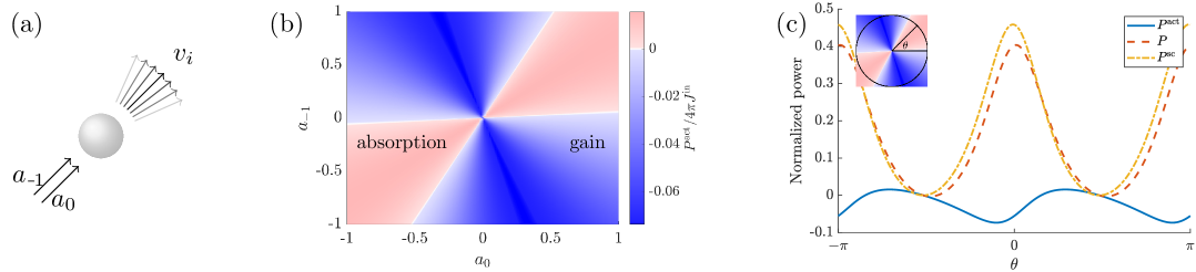
Figure 2: Energy phase diagram of $P^{\textrm{act}}$ for a single time-dependent point scatterer. We consider a situation with two incident harmonics $n=0$ and $n=-1$ as sketched in (a). Along the coordinate axes of (b), where one of the incident harmonics vanishes, we have $P^{\textrm{act}}<0$ and the total system has energy gain. When both harmonics are present, there are regimes of energy absorption, energy conservation, and energy gain. In (c), we plot the active, total, and scattered power, respectively, where the active power is given by the difference of the other two.

We note that the matrix $A$ might have low rank. For example, in the point-scattering approximation of [14], $A$ has rank $1$ close to a simple resonance. Zeros of $P^{\textrm{act}}$ therefore appear either when the two terms of (49) cancel, or when $a$ is a null vector of $A$. The former case can be viewed as a generalisation of the energy conservation of a non-absorbing time-invariant scatterer, where the extinguished power matches the scattered power. In the latter case, the incident field does not couple to the scatterer; the scattered field vanishes and $P^{\textrm{act}}=P=P^{\textrm{sc}}=0$ as highlighted in Fig. 3. Around this region, the total power may turn negative and the scatterer amplifies the total field in the forward direction of the incident wave.

It is worth emphasizing that the exhibited energy gain does not originate from instability of the system: The imaginary part of the resonant quasifrequencies remain negative and the solution does not exhibit an exponential growth as $t\to\infty$.

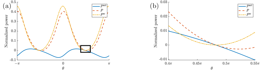
Figure 3: Since $A$ is low-rank, there may be points (shown in (b)) at which the scattered field vanishes. At these points, $P^{\textrm{act}}$ changes sign, signifying a transition from energy absorption to energy gain. Close to these points, the total energy $P$ may turn negative and the scatterer injects, rather than depletes, energy from the incident field.

For multiple point scatterers at positions $\mathbf{y}_{m}$, we use a fully-coupled approach to compute the scattered field. We take $N$ small particles defined by

$$D=\bigcup_{m=1}^{N}\epsilon B+\mathbf{y}_{m}.$$ (55)

The scattered field is then given by

$$v^{\textrm{sc}}_{i}(\mathbf{x})=\sum_{m=1}^{N}G^{k_{i}}(\mathbf{x}-\mathbf{y}_{m})\sum_{j=-\infty}^{\infty}\Lambda_{ij}\alpha_{jm},$$ (56)

where $\alpha_{jm}$ are the solutions of the fully-coupled linear system

$$\alpha_{im}=v^{\textrm{in}}_{i}(\mathbf{y}_{m})+\sum_{n\neq m}G^{k_{i}}(\mathbf{y}_{m}-\mathbf{y}_{n})\sum_{j=-\infty}^{\infty}\Lambda_{ij}\alpha_{jn}.$$ (57)

Computing the scattered and total power based on (43) and (48), we then have

$$P^{\textrm{sc}}=\sum_{i=-\infty}^{\infty}k_{i}\sum_{m,n=1}^{N}\overline{c_{im}}c_{in}\frac{\sin(k_{i}|\mathbf{y}_{n}-\mathbf{y}_{m}|)}{4\pi|\mathbf{y}_{n}-\mathbf{y}_{m}|},$$ (58)

and

$$P=\mathrm{Im}\sum_{i=-\infty}^{\infty}k_{i}\sum_{m=1}^{N}\overline{v^{\textrm{in}}_{i}}(\mathbf{y}_{m})c_{im},$$ (59)

where we use the shorthand $c_{im}=\sum\limits_{j=-\infty}^{\infty}\Lambda_{ij}\alpha_{jm}$. We illustrate these results in Fig. 4, where we plot the scattered field in a square configuration of point particles. We consider two values of $\theta$ as defined in Fig. 2(c), corresponding, respectively, to the cases $P^{\textrm{act}},P>0$ and $P^{\textrm{act}},P<0$. In the cases $P<0$, we note that $P^{\textrm{sc}}$ is close to zero, and the overall scattered has a low amplitude. In each case, the energy gain or absorption is amplified by including more resonators and is, in the case of well-separated resonators, directly proportional to the number of particles.

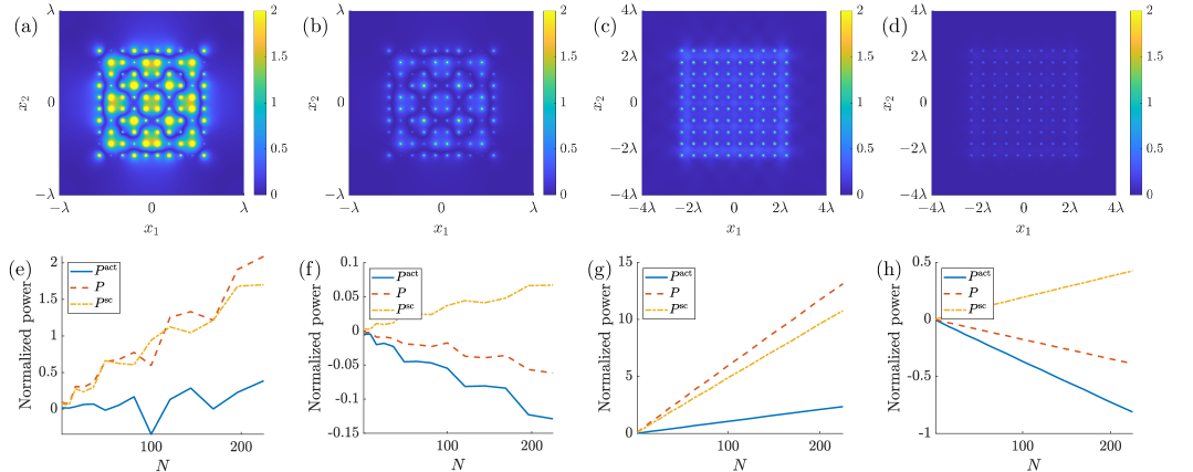
Figure 4: We plot examples of the scattered field ((a)–(d)) in a square configuration of scatterers, and corresponding normalized power ((e)–(h)) as a function of the number $N$ of particles, for two different values of $\theta$ as defined in Fig. 2. In (a),(b),(e),(f), we consider closely spaced scatterers (relative to the wavelength of the dominant harmonic). In this case, scattered modes hybridize and the collective response may be different compared to an isolated particle. For well-separated particles, the hybridization is negligible and the normalized powers $P^{\textrm{act}}$, $P$, and $P^{\textrm{sc}}$ are directly proportional to the number of particles.

VI Linear inverse scattering problem

We next consider linearized inverse scattering and reconstruction of the time-dependent material coefficient $\eta$. The reconstruction is based on measurements of the power $P$ and does not require measurements of the phases of the waves.

VI.1 Weak scattering approximation

We consider a perturbation regime of small $\eta$, in which case we can adopt a Born series approximation of the scattered field. To first-order approximation, the scattered field is then given by

$$v^{\textrm{sc}}_{i}(\mathbf{x})=k_{i}^{2}\int_{S^{2}}\sum_{j=-\infty}^{\infty}a_{j}(\hat{\mathbf{z}})\int_{D}G^{k_{i}}(\mathbf{x}-\mathbf{y})\eta_{i-j}(\mathbf{y})e^{\mathrm{i}\mkern 1.0muk_{j}\hat{\mathbf{z}}\cdot\mathbf{y}}\,\mathrm{d}\hat{\mathbf{z}}\,\mathrm{d}\mathbf{y}.$$ (60)

Similarly, we have a linearized Born approximation of the scattering amplitude $A$ as follows:

$$A_{ij}(\hat{\mathbf{x}},\hat{\mathbf{z}})=\frac{k_{i}^{2}}{4\pi}\int_{D}e^{-\mathrm{i}\mkern 1.0mu\left(k_{i}\hat{\mathbf{x}}-k_{j}\hat{\mathbf{z}}\right)\cdot\mathbf{y}}\eta_{i-j}(\mathbf{y})\,\mathrm{d}\mathbf{y},$$ (61)

in other words, that $A_{ij}(\hat{\mathbf{x}},\hat{\mathbf{z}})$ is given by the Fourier transform of $\eta_{i-j}$:

$$A_{ij}(\hat{\mathbf{x}},\hat{\mathbf{z}})=\frac{k_{i}^{2}}{4\pi}\widetilde{\eta}_{i-j}(k_{i}\hat{\mathbf{x}}-k_{j}\hat{\mathbf{z}}).$$ (62)

VI.2 Reconstruction without phase retrieval

Within the weak scattering approximation, we cannot reconstruct the real part of $\eta_{0}$ without phase retrieval, i.e., by solely measuring $P$. Nevertheless, as will be shown in this section, we are able to reconstruct $\eta_{i}$, for $i\neq 0$, based on (48). This will be made possible by taking an incident field composed of two plane waves of directions $\hat{\mathbf{z}}_{1},\hat{\mathbf{z}}_{2}$ and with distinct frequencies $k_{j_{1}}$ and $k_{j_{2}}$,

$$v^{\textrm{in}}_{i}(\mathbf{x})=c_{1}\delta_{ij_{1}}e^{\mathrm{i}\mkern 1.0muk_{i}\hat{\mathbf{z}}_{1}\cdot\mathbf{x}}+c_{2}\delta_{ij_{2}}e^{\mathrm{i}\mkern 1.0muk_{i}\hat{\mathbf{z}}_{2}\cdot\mathbf{x}}.$$ (63)

This gives

$$P(c_{1},c_{2})=\mathbf{c}^{*}M\mathbf{c},$$ (64)

where $\mathbf{c}=\begin{pmatrix}c_{1}\\ c_{2}\end{pmatrix}$, $Q=\frac{1}{2\mathrm{i}\mkern 1.0mu}\left(Q-Q^{*}\right)$, and the matrix $Q$ is given by

$$Q_{11} =k_{j_{1}}^{3}\int_{D}\eta_{0}(\mathbf{y})\,\mathrm{d}\mathbf{y}, Q_{12} =k_{j_{1}}^{3}\widetilde{\eta}_{j_{1}-j_{2}}(k_{j_{1}}\hat{\mathbf{z}}_{1}-k_{j_{2}}\hat{\mathbf{z}}_{2}),$$ (65)

$$Q_{21} =k_{j_{2}}^{3}\widetilde{\eta}_{j_{2}-j_{1}}(k_{j_{2}}\hat{\mathbf{z}}_{2}-k_{j_{1}}\hat{\mathbf{z}}_{1}), Q_{22} =k_{j_{2}}^{3}\int_{D}\eta_{0}(\mathbf{y})\,\mathrm{d}\mathbf{y}.$$ (66)

We consider the case $\mathrm{Im}\bigl{(}\eta(\mathbf{x},t)\bigr{)}=0$ and seek to reconstruct $\eta_{i}(\mathbf{x})$ for $i\neq 0$. We observe that $\widetilde{\eta}_{i}(\mathbf{k})=\overline{\widetilde{\eta}_{-i}(-\mathbf{k})}$. In this case, the off-diagonal term $\widetilde{\eta}_{j_{1}-j_{2}}(k_{j_{1}}\hat{\mathbf{z}}_{1}-k_{j_{2}}\hat{\mathbf{z}}_{2})$ can be reconstructed in the case $j_{1}\neq j_{2}$ using two measurements of $P$:

$$\widetilde{\eta}_{j_{1}-j_{2}}(k_{j_{1}}\hat{\mathbf{z}}_{1}-k_{j_{2}}\hat{\mathbf{z}}_{2})=\frac{1}{k_{j_{1}}^{3}-k_{j_{2}}^{2}}\bigl{(}P(1,\mathrm{i}\mkern 1.0mu)+\mathrm{i}\mkern 1.0muP(1,1)\bigr{)}.$$ (67)

We fix $j_{1}$ and $j_{2}$, and define the data function $D(\hat{\mathbf{z}}_{1},\hat{\mathbf{z}}_{2})$ as follows:

$$D(\hat{\mathbf{z}}_{1},\hat{\mathbf{z}}_{2})=\frac{1}{k_{j_{1}}^{3}-k_{j_{2}}^{3}}\bigl{(}P(1,\mathrm{i}\mkern 1.0mu)+\mathrm{i}\mkern 1.0muP(1,1)\bigr{)}.$$ (68)

Equation (67) then reads

$$D(\hat{\mathbf{z}}_{1},\hat{\mathbf{z}}_{2})=\int_{\mathbb{R}^{3}}\eta_{j_{1}-j_{2}}(\mathbf{x})e^{-\mathrm{i}\mkern 1.0mu(k_{j_{1}}\hat{\mathbf{z}}_{1}-k_{j_{2}}\hat{\mathbf{z}}_{2})\cdot\mathbf{x}}\,\mathrm{d}\mathbf{x}.$$ (69)

Equation (69) gives band-limited data of $\eta_{j_{1}-j_{2}}$ and provides means of (resolution-limited) reconstruction. We note that it is not necessary to measure the phases of the waves: in light of (61), knowledge of the scattering amplitude $A_{ij}(\hat{\mathbf{x}},\hat{\mathbf{z}})$ does not improve the reconstruction of $\eta_{i}(\mathbf{x})$ for $i\neq 0$.

The sampling set (in momentum space) is given by a “shell” of inner radius $k_{r}$ and outer radius $k_{R}$:

$$\left\{k_{j_{1}}\hat{\mathbf{z}}_{1}-k_{j_{2}}\hat{\mathbf{z}}_{2}\mid\hat{\mathbf{z}}_{1},\hat{\mathbf{z}}_{2}\in S^{2}\right\} =\left\{\mathbf{k}\in\mathbb{R}^{3}\mid k_{r}\leq|\mathbf{k}|\leq k_{R}\right\}$$ (70)

where

$$k_{r}=\Bigl{|}\left|k_{j_{1}}\right|-\left|k_{j_{2}}\right|\Bigr{|}\quad\text{and}\quad k_{R}=\left|k_{j_{1}}\right|+\left|k_{j_{2}}\right|.$$ (71)

In other words, we are able to reconstruct an upper and lower band-limited approximation of $\eta_{j_{1}-j_{2}}(\mathbf{x})$:

$$\eta_{j_{1}-j_{2}}(\mathbf{x})=\frac{1}{(2\pi)^{3}}\int_{k_{r}\leq|\mathbf{k}|\leq k_{R}}D(\mathbf{k})e^{\mathrm{i}\mkern 1.0mu\mathbf{k}\cdot\mathbf{x}}\,\mathrm{d}\mathbf{k}.$$ (72)

If both $k_{j_{1}}$ and $k_{j_{2}}$ are positive, we have

$$k_{r}=\frac{\left|j_{1}-j_{2}\right|\Omega}{c}\quad\text{and}\quad k_{R}=\frac{2\omega+(j_{1}+j_{2})\Omega}{c}.$$ (73)

The upper band limit corresponds to the usual resolution limit posed at the average of the two frequencies (incident and scattered) appearing in the measurement: instead of $d=\lambda/2$, the resolution limit $d$ is now

$$d=\frac{\lambda_{1}\lambda_{2}}{\lambda_{1}+\lambda_{2}},$$ (74)

where $\lambda_{1}$ and $\lambda_{2}$ are the wavelengths of the two harmonics.

The lower band limit depends purely on the modulation frequency $\Omega$ and not on the frequency of the incident and scattered waves. This gives an upper limit of the feature length that can be reconstructed, and the accuracy of the reconstruction depends heavily on the value of $\Omega$ in relation to the characteristic length scale $\ell$ of $\eta$. In a “slow-modulation” regime given by $\Omega\ell\ll 1$, the lower band limit is negligible and the reconstructed image is mainly governed by the regular resolution limit (c.f. Fig. 5(a)). On the other hand, in a “fast-modulation” regime given by $\Omega\ell\gg 1$, the lower band limit will severely restrict the reconstructed image (c.f. Fig. 5(c)), and image features of long length scales are invisible in the reconstructed image. In the intermediate regime, the reconstructed image is both upper and lower band-limited, and artifacts may appear in the reconstructed image (c.f. Fig. 5(b)).

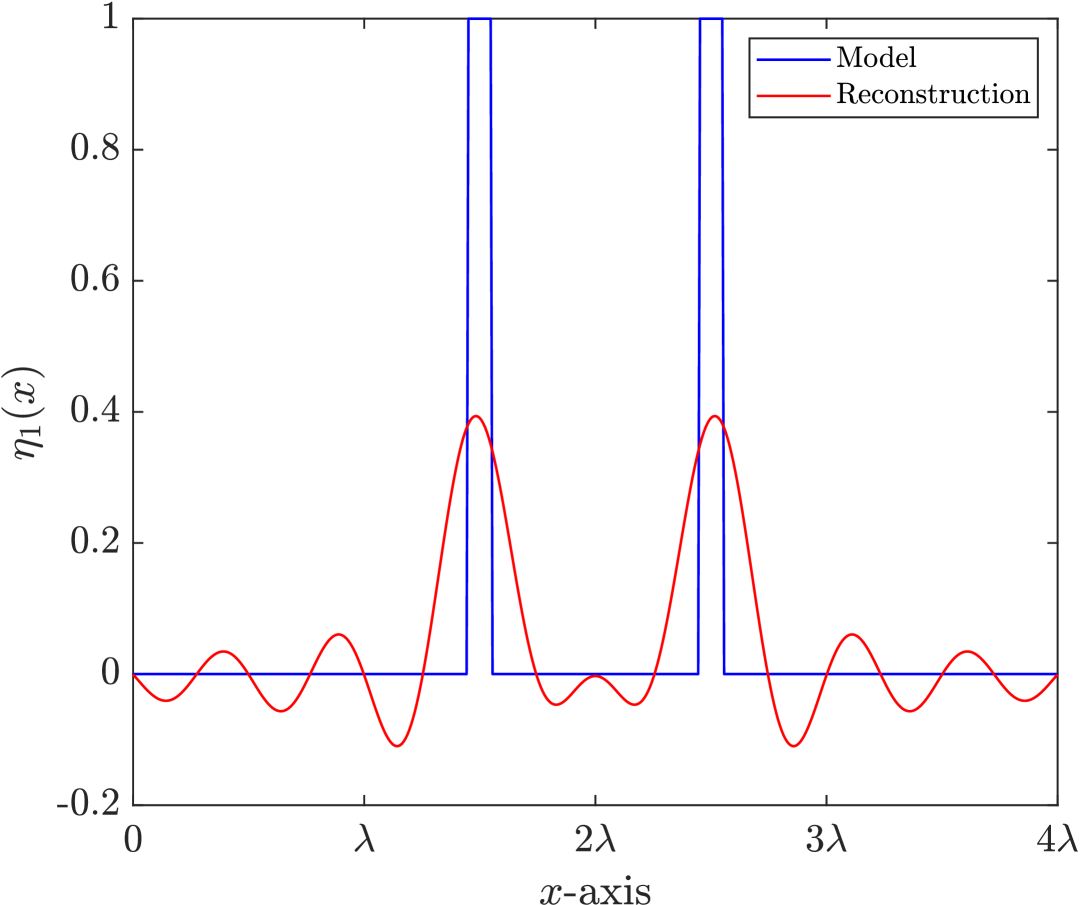
(a) $\Omega\ell=0.01$

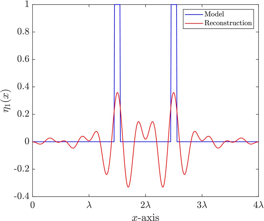
(b) $\Omega\ell=1$

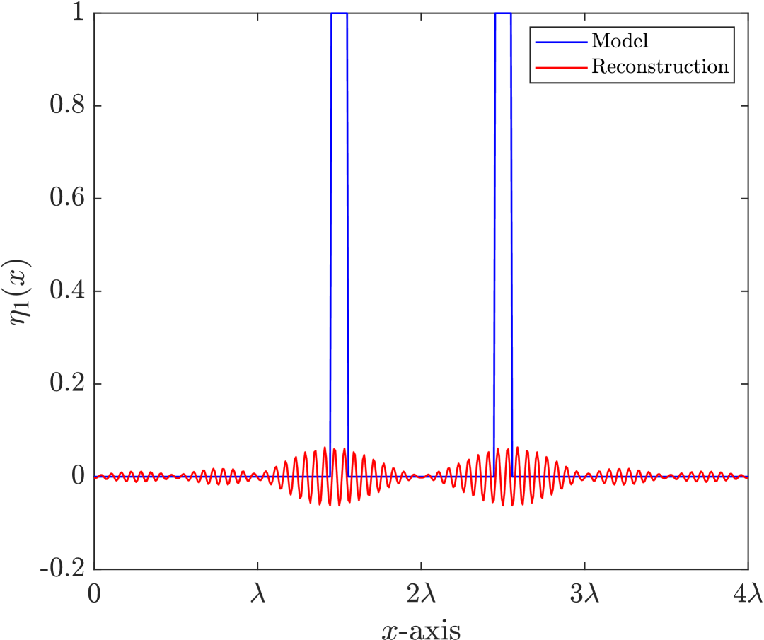
(c) $\Omega\ell=10$

Figure 5: One-dimensional example of a reconstructed image of $\eta_{1}(\mathbf{x})$ using a model with two piecewise constant “particles” of width $\ell=0.1\lambda$ and separation distance $d=\lambda$. If $\Omega\ell\ll 1$, it is possible to reconstruct the image up to the classical resolution limit given by (74). If $\Omega\ell\approx 1$, the reconstructed image is both upper and lower band-limited. If $\Omega\ell\gg 1$, the reconstruction fails.

VII Concluding remarks

We have studied the energy balance of a time-modulated material and derived an optical theorem for such systems. Our approach accounts for the broken energy conservation which arises due to frequency conversion, and we have shown that a conserved quantity is obtained by redefining the weights of the power of each frequency harmonic. We have seen that the same system might be subject to energy gain, energy absorption or energy loss, depending on the ratio of these harmonics present in the total field. We expect that these results will be significant for developing a general theory for energy-preserving spacetime metamaterials, with the goal to overcome instability and high energy cost associated to these systems. We have also shown how the optical theorem may be used as starting-point for image reconstruction, with upper and lower band limits, based on power measurements. We expect that the band limits may be mitigated using near-field microscopy, where the time-dependent sample is scanned by a probing tip in the near-field and the interaction between the tip and the sample is measured [25, 26]. This will be the topic of a forthcoming study.

References

• Holberg and Kunz [1966] D. Holberg and K. Kunz, Parametric properties of fields in a slab of time-varying permittivity, IEEE Transactions on Antennas and Propagation 14, 183 (1966).
• Koutserimpas et al. [2018] T. T. Koutserimpas, A. Alù, and R. Fleury, Parametric amplification and bidirectional invisibility in pt-symmetric time-floquet systems, Physical Review A 97, 013839 (2018).
• Zhang et al. [2024] J. Zhang, W. Donaldson, and G. P. Agrawal, Conservation law for electromagnetic fields in a space-time-varying medium and its implications, Physical Review A 110, 043526 (2024).
• Liberal et al. [2024] I. Liberal, A. Ganfornina-Andrades, and J. E. Vázquez-Lozano, Spatiotemporal symmetries and energy-momentum conservation in uniform spacetime metamaterials, ACS photonics 11, 5273 (2024).
• Zhang et al. [2023] J. Zhang, W. R. Donaldson, and G. P. Agrawal, Generalized energy conservation relation in a space-time varying medium, in 2023 Conference on Lasers and Electro-Optics (CLEO) (IEEE, 2023) pp. 1–2.
• Hirosawa and Wirth [2009] F. Hirosawa and J. Wirth, Generalised energy conservation law for wave equations with variable propagation speed, Journal of mathematical analysis and applications 358, 56 (2009).
• Ebert et al. [2015] M. R. Ebert, L. Fitriana, and F. Hirosawa, On the energy estimates of the wave equation with time dependent propagation speed asymptotically monotone functions, Journal of Mathematical Analysis and Applications 432, 654 (2015).
• Cullen [1958] A. Cullen, A travelling-wave parametric amplifier, Nature 181, 332 (1958).
• Raiford [1974] M. Raiford, Degenerate parametric amplification with time-dependent pump amplitude and phase, Phys. Rev. A 9, 2060 (1974).
• Koufidis et al. [2024] S. F. Koufidis, T. T. Koutserimpas, F. Monticone, and M. W. McCall, Enhanced scattering from an almost-periodic optical temporal slab, Physical Review A 110, L041501 (2024).
• Koutserimpas [2022] T. T. Koutserimpas, Parametric amplification interactions in time-periodic media: coupled waves theory, JOSA B 39, 481 (2022).
• Demkowicz et al. [2024] L. Demkowicz, J. M. Melenk, J. Badger, and S. Henneking, Stability analysis for electromagnetic waveguides. part 2: non-homogeneous waveguides, Advances in Computational Mathematics 50, 35 (2024).
• Yerezhep and Valagiannopoulos [2021] B. Yerezhep and C. Valagiannopoulos, Approximate stability dynamics of concentric cylindrical metasurfaces, IEEE Transactions on Antennas and Propagation 69, 5716 (2021).
• Hiltunen and Davies [2024] E. O. Hiltunen and B. Davies, Coupled harmonics due to time-modulated point scatterers, Physical Review B 110, 184102 (2024).
• Ammari et al. [2023] H. Ammari, J. Cao, E. O. Hiltunen, and L. Rueff, Transmission properties of time-dependent one-dimensional metamaterials, Journal of Mathematical Physics 64 (2023).
• Deshmukh and Milton [2022] K. J. Deshmukh and G. W. Milton, An energy conserving mechanism for temporal metasurfaces, Applied Physics Letters 121 (2022).
• Horsley and Pendry [2023] S. A. Horsley and J. B. Pendry, Quantum electrodynamics of time-varying gratings, Proceedings of the National Academy of Sciences 120, e2302652120 (2023).
• Carney et al. [2001] P. S. Carney, V. A. Markel, and J. C. Schotland, Near-field tomography without phase retrieval, Physical review letters 86, 5874 (2001).
• Govyadinov et al. [2009] A. A. Govyadinov, G. Y. Panasyuk, and J. C. Schotland, Phaseless three-dimensional optical nanoimaging, Physical review letters 103, 213901 (2009).
• Carney [1999] P. S. Carney, The optical cross-section theorem with incident fields containing evanescent components, journal of modern optics 46, 891 (1999).
• Carminati and Schotland [2021] R. Carminati and J. C. Schotland, Principles of scattering and transport of light (Cambridge University Press, 2021).
• Born and Wolf [2013] M. Born and E. Wolf, Principles of optics: electromagnetic theory of propagation, interference and diffraction of light (Elsevier, 2013).
• Fleury et al. [2016] R. Fleury, A. B. Khanikaev, and A. Alu, Floquet topological insulators for sound, Nature communications 7, 11744 (2016).
• Jones [1952] D. Jones, Removal of an inconsistency in the theory of diffraction, in Mathematical Proceedings of the Cambridge Philosophical Society, Vol. 48 (Cambridge University Press, 1952) pp. 733–741.
• Sun et al. [2006] J. Sun, P. S. Carney, and J. C. Schotland, Near-field scanning optical tomography: a nondestructive method for three-dimensional nanoscale imaging, IEEE Journal of selected topics in quantum electronics 12, 1072 (2006).
• Sun et al. [2007] J. Sun, P. S. Carney, and J. C. Schotland, Strong tip effects in near-field scanning optical tomography, Journal of Applied Physics 102 (2007).