Device-Free Localization with Multiple Antenna Receivers: Simulations and Results

Abstract

Device-Free Localization (DFL) is a passive radio method able to detect, estimate, and localize targets (e.g., human or other obstacles) that do not need to carry any electronic device. According to the Integrated Sensing And Communication (ISAC) paradigm, DFL networks exploit Radio Frequency (RF) devices, used for communication purposes, to evaluate also the excess attenuation due to targets moving in the monitored area, to estimate the target positions and movements. Several target models have been discussed in the literature to evaluate the target positions by exploiting the RF signals received by networked devices. Among these models, ElectroMagnetic (EM) body models emerged as an interesting research field for excess attenuation prediction using commercial RF devices. While these RF devices are usually single-antenna boards, the availability of low-cost multi-antenna devices e.g. those used in WLAN (Wireless Local Area Network) scenarios, allow us to exploit array-based signal processing techniques for DFL applications as well. Using an array-capable EM body model, this paper shows how to employ array-based processing to improve angular detection of targets. Unlike single-antenna devices that can provide only attenuation information, multi-antenna devices can provide both angular and attenuation estimates about the target location. To this end, simulations are presented and preliminary results are discussed. The proposed framework paves the way for a wider use of multi-antenna devices based, for instance, on WiFi6 and WiFi7 standards.

I Introduction

Device-Free Localization (DFL), a.k.a. passive radio localization, is a transformative framework designed to detect, localize, and track people (or objects) in a 3-D area illuminated by Radio Frequency (RF) signals of opportunity. According to the Integrated Sensing and Communication (ISAC) paradigm [1], the same RF devices used for communications can be leveraged by DFL systems to transform each RF device into a virtual sensor for passive sensing operations.

For instance, a network of these RF communication devices can be usefully exploited to evaluate the presence and the location of people by using info from the received ElectroMagnetic (EM) field. In fact, both presence and movements of people or objects, namely the targets, modify the incident EM field [2] that is already collected and processed by the RF devices to provide a reliable communication. The alterations of the received RF signals does not only impair the radio communication channel, but can be also specifically processed for localization purposes to estimate target information such as presence, location, posture, movements, and size [1, 3].

Body models have been presented and widely discussed in the literature for single-antenna devices for both single-target [4, 5, 6] and multi-targets [7] DFL scenarios. Moreover, different radio channel measurements, such as Channel State Information (CSI), Received Signal Strength (RSS), Angles of Arrival (AoA) and Time of Flight (ToF) [1], have been exploited for DFL applications according to different processing frameworks such as radio imaging [4], Bayesian tracking [1], fingerprinting methods [1], Compressive Sensing algorithms [8], and Machine Learning/Deep Learning (ML/DL) systems [3].

The concomitant wide diffusion of multi-antenna WLAN devices, such as those designed according to the WiFi6 and WiFi7 standards, and the development of CSI extraction tools [9], have sped up the research activities about multi-antenna DFL systems with the adoption of multi-antenna CSI-based processing methods [10, 11].

A few references only focus on multi-antenna models: [12] employs a very simple propagation model while [13] deals with a computational-intensive Ray Tracing (RT) approach not suitable for real-time DFL applications. Actually, EM-based simulators can be exploited for modeling as well. However, they are usually too complex and very slow to be of practical use for real-time DFL [6, 7].

This paper extends the physical-statistical body model proposed by the authors in [14, 15] to predict the body-induced propagation losses using RF devices with multiple receiving antennas. The array-based body model is exploited to simulate a target moving in the monitored area and to provide an estimate of the AoA of the perturbed RF waves due to the moving target.

The paper is organized as follows: in Sect. II, the array-based EM body model for applications with multiple receiving antenna devices is briefly recalled. Then, Sect. III shows the array-based processing method to identify the AoA of the RF signals that are altered by the presence of the target. Sect. IV presents some preliminary simulation results while Sect. V shows some preliminary conclusions and proposes future activities.

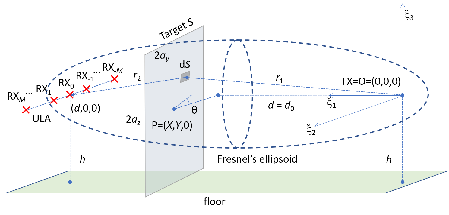
Figure 1: Single-link 3-D layout of an ULA with $2M+1$ receiving antennas. The array is deployed along a line at distance $d=d_{0}$ from the TX and orthogonal to the LoS path connecting the $TX$ with the $RX_{0}$ device.

II EM body model with multiple RX antennas

According to the scalar diffraction framework adopted in [6], we briefly recall here the EM multi-antenna body model proposed in [14, 15] for a single-link scenario. Fig. 1 shows the layout composed by an Uniform Linear Array (ULA) of $2M+1$ isotropic receiver antennas RX_m, with$-M\leq m\leq M$ and $M,\,m\in\mathbb{Z}$, a single isotropic transmitting antenna TX, and a single-target $S$ that moves in the monitored area near the radio link. Each m-th antenna RX_m of the array is uniformly placed at mutual distance $d_{a}$ along a segment orthogonal to the Line-of-Sight (LoS) at distance $d=d_{0}$ from the TX and horizontally placed at distance $h$ w.r.t. the floor. The central antenna is indicated by the index $m=0$. We assume here that the floor has no influence on the RF signals. If this assumption does not hold true, the proposed model can easily be extended as shown in [16]. The 2-D footprint of the 3-D deployment of Fig. 1 is also depicted in Fig. 2.

II-A Body model

Considering DFL applications, we assume two main configurations: the first one refers to the empty environment (i.e., the free-space case, namely $\mathcal{S}=0$) while, in the second scenario, the target $S$ is present in the monitored area ($\mathcal{S}=1$). The target is sketched [6, 7] as a vertical standing EM absorbing 2-D sheet $S$ of height $2a_{z}$ and traversal size $2a_{y}$ that is rotated of the angle $\theta$ w.r.t. the $\xi_{2}$ axis as shown in Figs. 1 and 2. Assuming a negligible mutual antenna coupling, approximately valid for $d_{a}>\lambda/4$, the electric field $E^{\left(m\right)}$ received by the m-th antenna of the array, is:

$$\begin{array}[]{ll}\frac{E^{\left(m\right)}}{E_{R}^{\left(m\right)}}=&1-j\frac{d_{m}}{\lambda}{\displaystyle\intop_{S}}\frac{1}{r_{1,m}r_{2,m}}\cdot\\ &\cdot\exp\left\{-j\frac{2\pi}{\lambda}\bigl{(}r_{1,m}+r_{2,m}-d_{m}\bigr{)}\right\}d\xi_{2}\,d\xi_{3},\end{array}$$ (1)

where $E_{R}^{\left(m\right)}$ is the EM field received by the same $RX_{m}$ device in the reference condition $\mathcal{S}=0$. The term $d_{m}$ indicates the distance of the m-th antenna $RX_{m}$ of the array from the TX while $d_{1,m}$ and $d_{2,m}$ are the distances of the projection point $O_{m}^{{}^{\prime}}$ of the barycenter $P$ of the 2-D surface $S$ from the TX and $RX_{m}$ nodes, respectively. Likewise, $r_{1,m}$ and $r_{2,m}$ are the distances of the generic elementary area $dS$ of the target $S$ from the TX and the $RX_{m}$, respectively. Integration is performed in (1) over the squared domain $S$ having height $2a_{z}$ and traversal size $2a_{y}$. $P(X,Y,Z)$ indicates the target location coordinates. For simplicity, $Z$ is then dropped since it is implicitly assumed $Z=0$.

For $M=0$, the equation (1) reduces to the single-antenna case [6] where RX₀ coincides with the RX antenna at distance $d=d_{0}$ from the TX. The excess attenuation [6] at RX_m, due to the influence of the target $S$ w.r.t. the free-space scenario, is computed [6] as $A_{T}^{\left(m\right)}=P_{R}^{\left(m\right)}/P^{\left(m\right)}=\left|E_{R}^{\left(m\right)}/E^{\left(m\right)}\right|^{2}$ where $P_{R}^{\left(m\right)}$ and $P^{\left(m\right)}$ are the received power at RX_m without and with a target in the link area, respectively. Usually, the excess attenuation is given in dB as $A_{T,dB}^{\left(m\right)}=10\,\log_{10}\left|E_{R}^{\left(m\right)}/E^{\left(m\right)}\right|^{2}$. The ratio $E_{R}^{\left(m\right)}/E_{R}^{\left(0\right)}$ is given by:

$$\begin{array}[]{ll}\frac{E_{R}^{\left(m\right)}}{E_{R}^{\left(0\right)}}=&\frac{d_{0}}{d_{m}}\,\exp\left\{-j\frac{2\pi}{\lambda}\bigl{(}d_{m}-d_{0}\bigr{)}\right\},\end{array}$$ (2)

where $E_{R}^{\left(0\right)}$ is the electric field received by the central antenna $RX_{0}$ that is on the LoS path at distance $d_{0}$ from the TX. Eq. (1) can be rewritten as:

$$\begin{array}[]{ll}\frac{E^{\left(m\right)}}{E_{R}^{\left(0\right)}}=&\frac{d_{0}}{d_{m}}\,\exp\left\{-j\frac{2\pi}{\lambda}\left(d_{m}-d_{0}\right)\right\}\bigl{[}1-j\frac{d_{m}}{\lambda}{\displaystyle\intop_{S}}\frac{1}{r_{1,m}r_{2,m}}\cdot\bigr{.}\\ &\bigl{.}\cdot\exp\left\{-j\frac{2\pi}{\lambda}\left(r_{1,m}+r_{2,m}-d_{m}\right)\right\}d\xi_{2}\,d\xi_{3}\bigr{]}.\end{array}$$ (3)

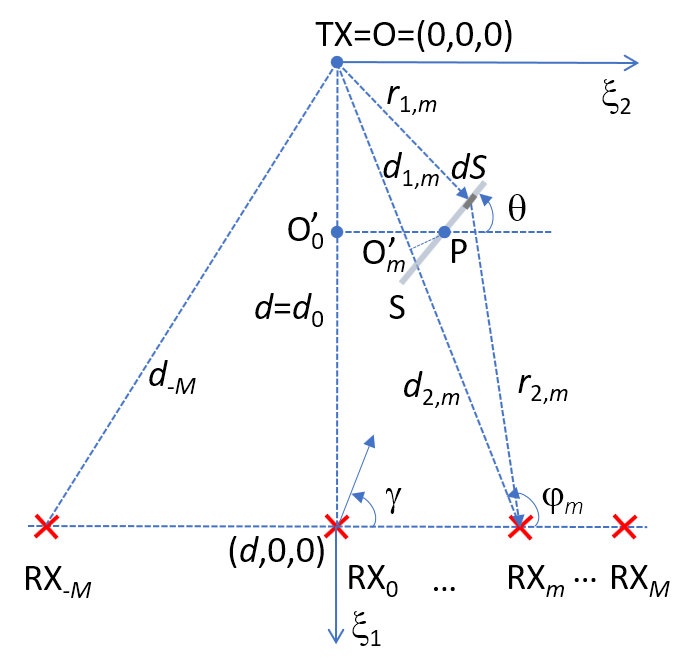
Figure 2: 2-D layout of the radio link of Fig. 1. The point $O_{m}^{{}^{\prime}}$ is the projection of the barycenter $P$ of the target $S$ over the m-th LoS path having length $d_{m}$.

According to (2) and (3), the m-th component of the received vector $\mathbf{r}\left(t,\mathcal{S}\right)=\left[r_{-M}\left(t,\mathcal{S}\right)\,...\,r_{-1}\left(t,\mathcal{S}\right)\,r_{0}\left(t,\mathcal{S}\right)\,r_{1}\left(t,\mathcal{S}\right)\,...\,r_{M}\left(t,\mathcal{S}\right)\right]^{T}$ of size $2M+1$ is defined as:

$$r_{m}\left(t,\mathcal{S}\right)=\left\{\begin{array}[]{ll}E_{R}^{\left(m\right)}+n_{m}=E_{R}^{\left(0\right)}\,\frac{E_{R}^{\left(m\right)}}{E_{R}^{\left(0\right)}}+n_{m}&\textrm{if $\mathcal{S}=0$}\\ E^{\left(m\right)}+n_{m}=E_{R}^{\left(0\right)}\,\frac{E_{R}^{\left(m\right)}}{E_{R}^{\left(0\right)}}\,\frac{E^{\left(m\right)}}{E_{R}^{\left(m\right)}}+n_{m}&\textrm{if $\mathcal{S}=1$}\end{array}\right.$$ (4)

where $n_{m}$ is the m-th component of the Additive White Gaussian Noise (AWGN) complex vector $\mathbf{n}\left(t\right)=\left[n_{-M}\left(t\right)\,...\,n_{-1}\left(t\right)\,n_{0}\left(t\right)\,n_{1}\left(t\right)\,...\,n_{M}\left(t\right)\right]^{T}$ of size $2M+1$, that is assumed to be spatially white with zero mean and covariance $\sigma_{n}^{2}\mathbf{I}$.

The interested reader can refer to [1, 6, 7] for further information and discussions about the noise effects with and without the presence of a target inside the monitored area.

II-B Beamforming

Being $\boldsymbol{w}=\left[w_{-M}\,...\,w_{0}\,...\,w_{M}\right]^{T}$ the beamforming vector of size $2M+1$ collecting all linear beamforming coefficients, the output $y=y\left(t,\mathcal{S}\right)$ of linear beamforming processing is equal to:

$$y\left(t,\mathcal{S}\right)=\sum_{m=-M}^{+M}w_{m}^{*}\,r_{m}\left(t,\mathcal{S}\right)=\mathbf{w}^{H}\mathbf{r}\left(t,\mathcal{S}\right),$$ (5)

where $\left(\cdot\right)^{*}$ indicates the conjugate operator and $\left(\cdot\right)^{H}$ the Hermitian operator, while $r_{m}\left(t,\mathcal{S}\right)$ is the EM field received in the $RX_{m}$ antenna.

In DFL scenarios, we are interested in evaluating the power $P_{y}\left(\mathcal{S}\right)$ of the signal $y$ with or without the target $S$. This is given by:

$$\begin{array}[]{ll}P_{y}\left(\mathcal{S}\right)&=\mathbb{E}\left[y\left(t,\mathcal{S}\right)\,y^{*}\left(t,\mathcal{S}\right)\right]\\ &=\mathbf{w}^{H}\,\mathbf{R}\left(\mathcal{S}\right)\,\mathbf{w}\end{array}$$ (6)

where matrix $\mathbf{R}\left(\mathcal{S}\right)=\mathbb{E}\left[\mathbf{r}\left(t,\mathcal{S}\right)\,\mathbf{r}^{H}\left(t,\mathcal{S}\right)\right]$ of size $\left(2M+1\right)\times\left(2M+1\right)$ is the autocorrelation matrix of $\mathbf{r}\left(t,\mathcal{S}\right))$.

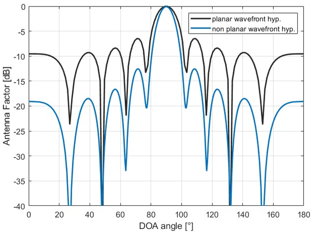
Figure 3: Comparisons of the array factors for an ULA composed by $9$ antennas ($M=4$) uniformly spaced at $d_{a}=\lambda/2$ with planar and non planar wave propagation hypotheses. For the non planar assumption, it is also $d_{0}=d$ and $d_{m}=\sqrt{d_{0}^{2}+m^{2}d_{a}^{2}}$ with $d=4$ m.

III Impact of body effects on indoor beamforming

The presence of the target generates perturbations in the beamforming response, occasionally altering the direction of maximum received radiation. This effect is analyzed in this section because of its relevance to passive localization applications.

In addition to discussing the effects of body motions on indoor beamforming response, we also propose an estimation algorithm to evaluate the direction of arrival (DoA) $\gamma$ of the electromagnetic wave when a target is present on the scene. To this aim, (4) can be rewritten as:

$$\mathbf{r}\left(t,\mathcal{S}\right)=\left\{\begin{array}[]{ll}E_{R}^{\left(0\right)}\,\mathbf{a}+\mathbf{n}&\textrm{if $\mathcal{S}=0$}\\ E_{R}^{\left(0\right)}\,\textrm{diag$\left(\mathbf{a}\right)$}\,\mathbf{E}_{r}+\mathbf{n}=&\textrm{if $\mathcal{S}=1$,}\end{array}\right.$$ (7)

where the column vector $\mathbf{E}_{r}$ of size $2M+1$ represents the electric field ratio (1) received by the antenna array for $\mathcal{S}=1$. It is defined as $\mathbf{E}_{r}=\left[E^{\left(-M\right)}/E_{R}^{\left(-M\right)}\,...\,E^{\left(M\right)}/E_{R}^{\left(M\right)}\right]^{T}$.

The steering vector $\mathbf{a}$ depends on the propagation assumptions: for planar wave propagation, it is, for $-M\leq m\leq M$:

$$\mathbf{a}=\left[\exp\left\{j\,m\,\frac{2\pi}{\lambda}d_{a}\cos\gamma\right\}\right].$$ (8)

Since DFL applications are mostly deployed in indoor scenarios with short links, the planar wavefront assumption [18] adopted for far-field scenarios is an approximation of the true behavior. Thus, the correct steering vector is equal to [7]:

$$\mathbf{a}=\left[\frac{d_{0}}{d_{m}}\,\exp\left\{j\,m\,\frac{2\pi}{\lambda}d_{a}\frac{\cos\left\{\left(\gamma+\varphi_{m}\right)/2\right\}}{\cos\left\{\left(\gamma-\varphi_{m}\right)/2\right\}}\right\}\right],$$ (9)

where $\varphi_{m}$ is the angle formed by the LoS of the m-th array antenna with the $\xi_{2}$ axis. For $-M\leq m\leq M$, it is $\varphi_{m}=\arcsin\left\{\left(d_{0}/d_{m}\right)\,\sin\gamma\right\}$. Moreover, it is also $\left|\mathbf{a}\right|^{2}=\sum_{m=-M}^{M}\left(d_{0}/d_{m}\right)^{2}$ and $\varphi_{0}=\gamma$.

The array factor $F_{a}=\mathbf{w}^{T}\mathbf{a}\left(\gamma\right)$ defines the response of the array as a function of the selected beamforming coefficients $\mathbf{w}$ and of the incident angle $\gamma$ of the steering vector $\mathbf{a}\left(\gamma\right)$. According to the selected outdoor (i.e., long or very long LoS path) or indoor (i.e., short LoS path) scenarios, corresponding to planar vs non-planar hypotheses, respectively, (10) and Fig. 3 summarize the analytical and graphical assumptions.

$$F_{a}=\left\{\begin{array}[]{ll}\frac{1}{2M+1}{\displaystyle\sum_{m=-M}^{+M}}\exp\{{jm\frac{2\pi}{\lambda}d_{a}\cos\gamma}\}&\thinspace\textrm{planar hyp.}\\ \frac{1}{2M+1}{\displaystyle\sum_{m=-M}^{+M}}\frac{d_{0}}{d_{m}}\,\cdot\\ \cdot\exp\left\{j\,m\,\frac{2\pi}{\lambda}d_{a}\frac{\cos\left\{\left(\gamma+\varphi_{m}\right)/2\right\}}{\cos\left\{\left(\gamma-\varphi_{m}\right)/2\right\}}\right\}&\thinspace\textrm{non-planar hyp.}\end{array}\right.$$ (10)

However, to exploit (9), all distances $d_{m}$ must be a priori known. For this reason, in this paper, we assume as a starting hypothesis the approximation (8) for $\mathbf{w}$. Other assumptions and methods can be adopted, but these are outside the scope of this paper.

As assumed for the single-antenna case [6], but differently from what suggested in [7], in this paper we assume that the mean excess attenuation $A_{T}$ corresponds to the ratio between the power terms $P_{0}\left(\mathcal{S}=0\right)=\mathbb{E}\left[r_{0}\left(t,\mathcal{S}=0\right)r_{0}^{*}\left(t,\mathcal{S}=0\right)\right]$ and $P_{y}\left(\mathcal{S}=1\right)$. $P_{0}\left(\mathcal{S}=0\right)$ is the power received by the central antenna of the array (i.e., $m=0$) when there are no targets within the monitored area.

By neglecting the noise terms, the excess attenuation is given by $A_{T,dB}=10\log_{10}\frac{P_{0}\left(\mathcal{S}=0\right)}{P_{y}\left(\mathcal{S}=1\right)}$.

To locate the target, we estimate the angle of arrival $\hat{\gamma}$, namely the angle/direction of maximum received power w.r.t the empty environment, with no subjects in the monitored area:

$$\hat{\gamma}=\arg\max_{0\leq\gamma\leq\pi}\frac{P_{y}\left(\mathcal{S}=1\right)}{P_{0}\left(\mathcal{S}=0\right)}$$ (11)

that maximizes the power ratio $P_{y}/P_{0}$ by using (7) and the steering vector $\mathbf{a}\left(\gamma\right)$ given by (8). Then, the corresponding value of $A_{T,dB}=A_{T,dB}\left(\hat{\gamma}\right)$ is evaluated, as well.

With respect to [6], the use of an antenna array allows us to estimate two target information: the excess attenuation due to the target and the DoA of the received signals that are distorted by the target. It is worth noticing that the DoA of the received signals is influenced by the target but does not coincide with the one due to the location of the target.

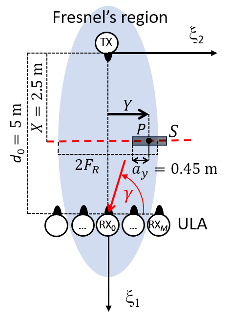
Figure 4: Link layout used for the simulations: the antenna array is composed by 5 antennas ($M=2$) while the target $S$, with size $a_{z}=0.9$ m and $a_{y}=0.45$ m, is placed in different positions along the line having distance $x=2.5$ m from the TX.

IV Simulation results

In this section, we introduce the simulation setup and show some preliminary results obtained according to the criterion (11).

The carrier frequency $f_{c}$ is set to $f_{c}=2.4868$ GHz (i.e., $\lambda=12$ cm), and we used an ULA composed of $5$ omni-directional antennas ($M=2$) uniformly spaced at $d_{a}=\lambda/2$ as shown in the layout sketch described in Fig. 4. The length of the central link of the array (i.e., for $m=0$) is equal to $d=d_{0}=5$ m while all links of the array are horizontally placed at height $h=0.9$ m from the ground. The minor semi-axis of the first Fresnel’s ellipsoid $F_{R}=\sqrt{\lambda\,d}/2$ is equal to $F_{R}=0.39$ m. We also assume that there are no reflections or other multi-path effects due to the presence of floor, walls, and ceiling.

As far as the body model is concerned, the absorbing 2-D sheet that represents the target has size $a_{z}=0.9$ m and $a_{y}=0.45$ m (i.e. corresponding to a total size of $1.80$ m $\times$ $0.90$ m). The target is placed vertically on the floor, that is used only to support the target and does not have any EM influence on the radio links. The LoS of the central link will be the reference LoS line for the target positions with the origin of the axes placed in the TX as shown in Fig. 4.

It is well-known [6, 7] that a target influences the received field only when it is near the radio link. The same behavior is apparent also here as shown in Figs. 5 and 6 where the received power ratio $P_{y}\left(\mathcal{S}=1\right)/P_{0}\left(\mathcal{S}=0\right)$ is depicted as a function of $\gamma$.

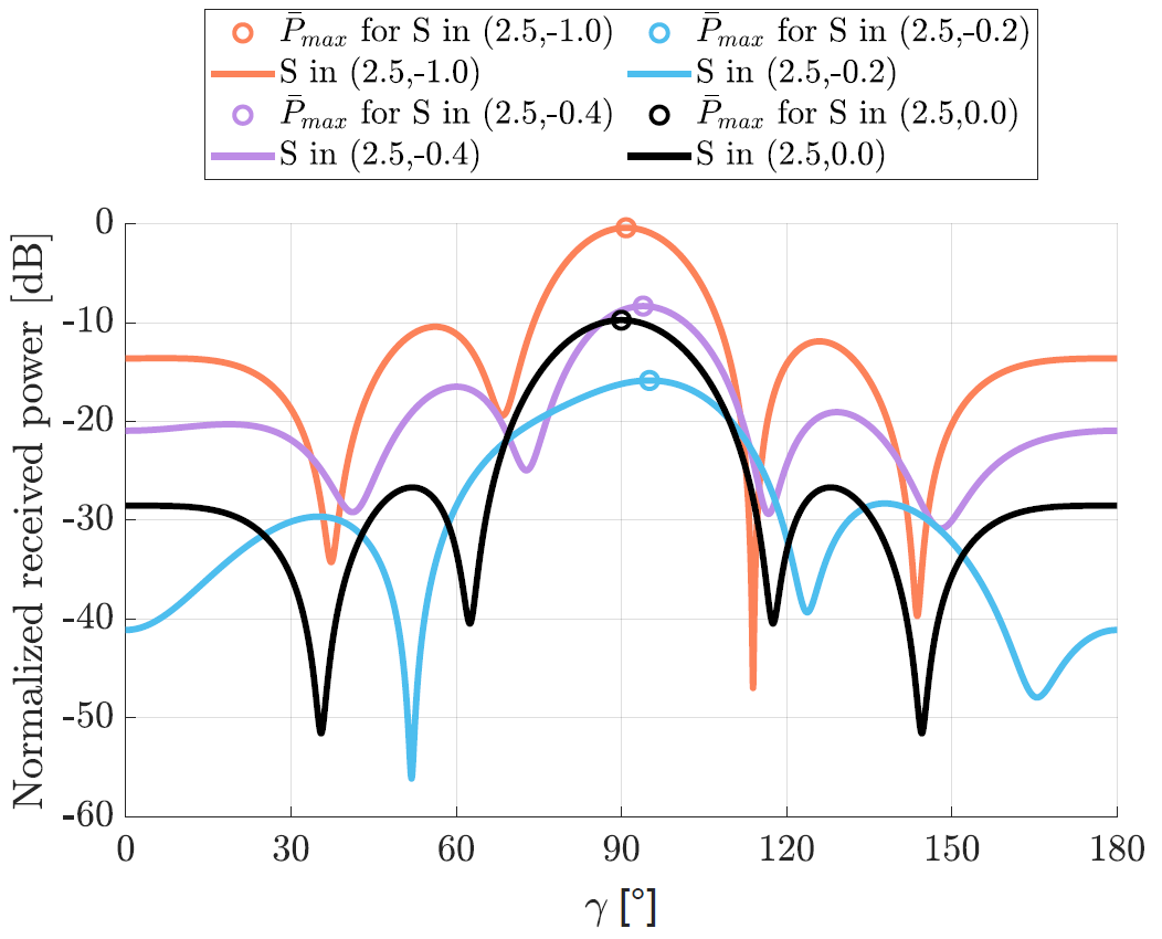
Figure 5: The received power ratio $P_{y}\left(\mathcal{S}=1\right)/P_{0}\left(\mathcal{S}=0\right)$ as a function of $\gamma$ and different target positions: the orange line indicates a target in (2.5,-1.0), the purple line in (2.5,-0.4), the blue line in (2.5,-0.2), and the black line in (2.5,0.0). The small circles indicate the maximum values of the received power ratio.

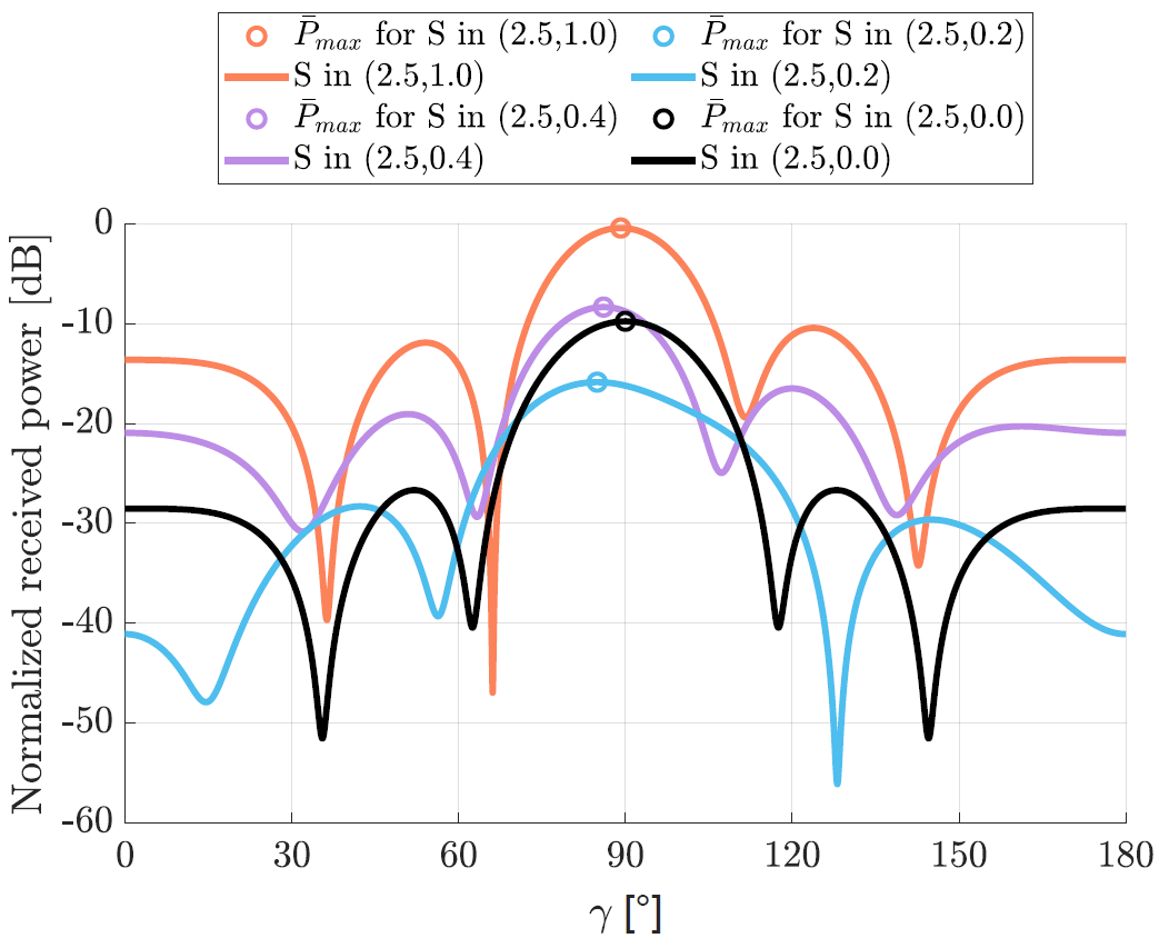
Figure 6: The received power ratio $P_{y}\left(\mathcal{S}=1\right)/P_{0}\left(\mathcal{S}=0\right)$ as a function of $\gamma$ and different target positions: the orange line indicates a target in (2.5,1.0), the purple line in (2.5,0.4), the blue line in (2.5,0.2), and the black line in (2.5,0.0). The small circles indicate the maximum values of the received power ratio.

It is apparent that the proposed method is capable of discriminating between targets placed on the left side of the link i.e. for $\pi/2<\gamma\leq\pi$ (Fig. 5) or right side of the link i.e. for $0\leq\gamma<\pi/2$ (Fig. 6) at least for an interval around $(\pi/2,0)$ in the $\gamma-Y$ space. This capability cannot be implemented for a single-antenna receiver that shows a perfect symmetry of the received power ratio w.r.t. the LoS path [6].

Fig. 7 shows the comparison between the true $\gamma$ and the estimated $\hat{\gamma}$ values for target positions close to the link. It is worth noticing that, for this example, the size of the Fresnel’s ellipsoid is the Y interval $[-0.39,+0.39]$ m and the side discrimination capability interval is approximately the same.

Fig. 8 shows the excess attenuation in dB corresponding to the $\hat{\gamma}$ values shown in Fig. 7. It has to be noted that this side discrimination capability can be exploited only for target close to the radio links since these links are not influenced by distant target as apparent in Fig. 8 due to very small values of the excess attenuation for $|Y|>1$ m.

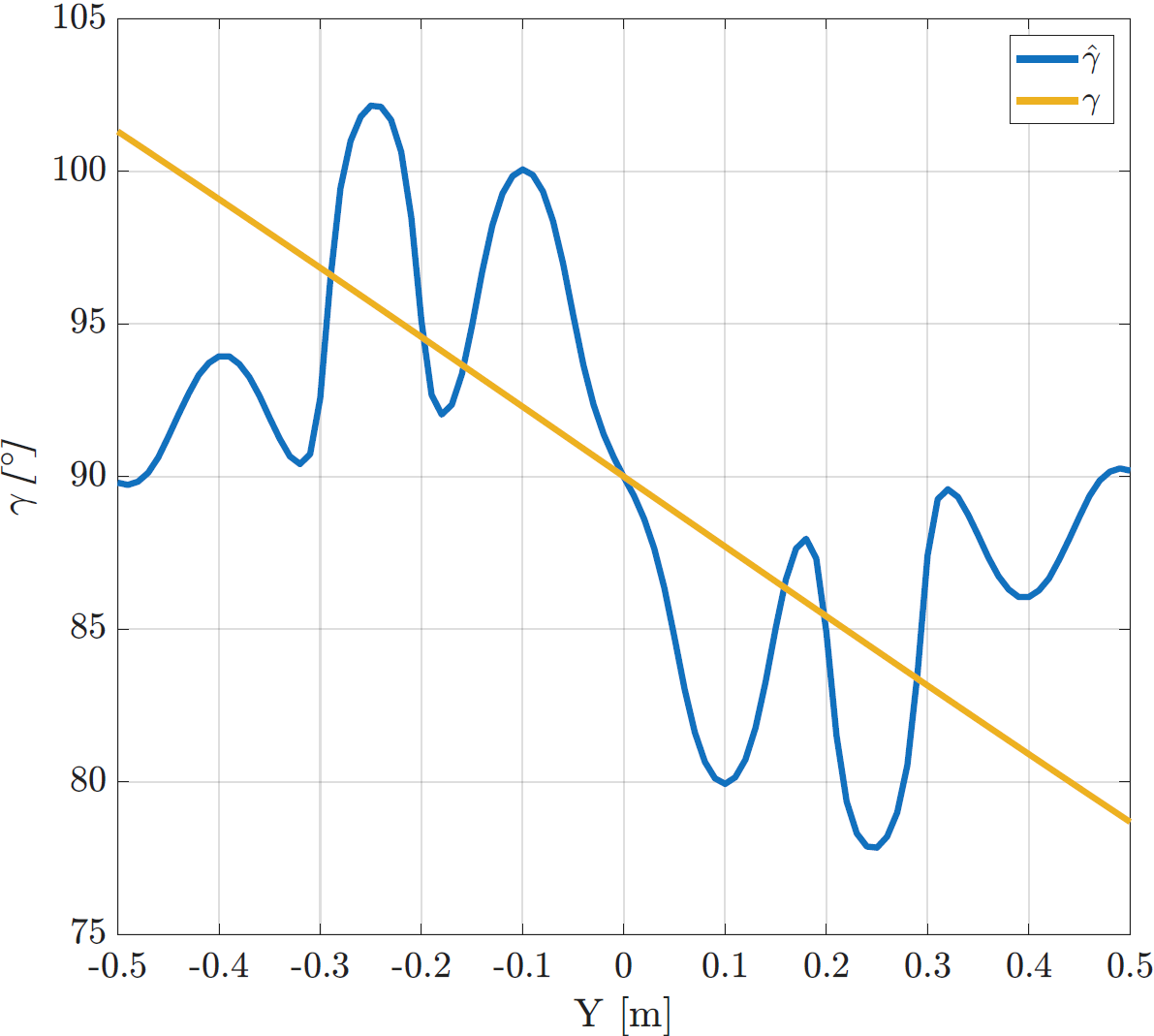
Figure 7: Estimated ($\hat{\gamma}$) vs true ($\gamma$) values of the angle of arrival for different target positions located in (2.5,Y) with varying Y.

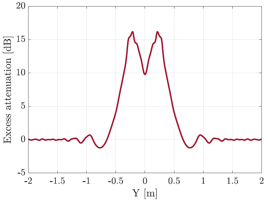
Figure 8: Excess attenuation for the different target positions located in (2.5,Y) with varying Y. These values are obtained for the $\hat{\gamma}$ values of Fig. 7. To show the slow damping of the excess attenuation, the Y interval is larger than the one of Fig. 7.

V Conclusions

In this paper, we introduce a body model for linear antenna arrays capable of inferring both the presence of a target in the surrounding of the radio link, and also the angular information, namely the Direction of Arrival (DoA). In fact, the received signals that are distorted by the target, reveal the offset position of the same target w.r.t. the array line-of-sight path. The model is relevant for Device-Free Localization (DFL) applications.

Unlike single-antenna links that can only evaluate body-induced attenuation effects in the monitored area covered by the radio links, the multi-antenna array is able to evaluate both attenuation and Angle-of-Arrival (AoA) information.

The presence of the target deforms the received ElectroMagnetic (EM) field w.r.t. the free-space configuration and this distortion can be used to estimate angular positioning information. This AoA-related capability paves the way to the use of array-based sensing methods for more accurate passive localization as well as object detection systems.

References

- [1] S. Savazzi, et al., ”Device-free Radio Vision for assisted living: leveraging wireless channel quality information for human sensing,” IEEE Signal Processing Magazine, vol. 33, no. 2, pp. 45–58, Mar. 2016.
- [2] G. Koutitas, ”Multiple human effects in body area networks,” IEEE Antennas and Wireless Propagation Letters, vol. 9, pp. 938–941, 2010.
- [3] R.C. Shit, et al., ”Ubiquitous Localization (UbiLoc): A Survey and Taxonomy on Device Free Localization for Smart World,” IEEE Communications Surveys & Tutorials, vol. 21, no. 4, pp. 3532–3564, Fourthquarter 2019.
- [4] J. Wilson, et al., ”Radio tomographic imaging with wireless networks,” IEEE Trans. on Mobile Comp., vol. 9, no. 5, pp. 621–632, May 2010.
- [5] M. Mohamed, et al., ”Physical-statistical channel model for off-body area network,” IEEE Antennas and Wireless Propagation Letters, vol. 16, pp. 1516–1519, 2017.
- [6] V. Rampa, et al., ”EM Models for Passive Body Occupancy Inference,” IEEE Antennas and Wireless Propagation Letters, vol. 16, pp. 2517-2520, 2017.
- [7] V. Rampa, et al., ”Electromagnetic Models for Passive Detection and Localization of Multiple Bodies”, IEEE Transactions on Antennas and Propagation, vol. 70, no. 2, pp. 1462–1745, 2022.
- [8] J. Wang, et al., ”Device-free localisation with wireless networks based on compressive sensing,” IET Communications, vol. 6, no. 5, pp. 2395–2403, Oct. 2012.
- [9] M. Atif, et al., ”Wi-ESP—A tool for CSI-based Device-Free Wi-Fi Sensing (DFWS),” Journal of Computational Design and Engineering, vol. 7, no. 5, pp. 644–656, Oct. 2020.
- [10] S. Shukri, et al., Enhancing the radio link quality of device-free localization system using directional antennas,” Proc. of the 7th International Conference on Communications and Broadband Networking, pp. 1–5, Apr. 2019.
- [11] D. Garcia, et al., ”POLAR: Passive object localization with IEEE 802.11 ad using phased antenna arrays,” Proc. of the IEEE INFOCOM 2020-IEEE Conference on Computer Communications, pp. 1838–1847, Jul. 2020.
- [12] W. Ruan, et al., ”Device-free indoor localization and tracking through Human-Object Interactions,” Proc. of the IEEE 17th International Symposium on A World of Wireless, Mobile and Multimedia Networks (WoWMoM’16), Coimbra, pp. 1–9, Jun. 2016.
- [13] V. Ojeda, et al., ”Rx position effect on Device Free Indoor Localization in the 28 GHz band,” Proc. of the IEEE Sensors Applications Symposium (SAS’2022), Sundsvall, pp. 1–6, Aug. 2022.
- [14] V. Rampa et al., ”Electromagnetic Models for Device-Free Radio Localization with Antenna Arrays,” Proc. of the IEEE-APS Topical Conf. on Antennas and Propagation in Wireless Communications, pp. 1–6, Sept. 2022.
- [15] V. Rampa et al., ”An EM Body Model for Device-Free Localization with Multiple Antenna Receivers: A First Study,” Proc. of the IEEE-APS Topical Conf. on Antennas and Propagation in Wireless Communications, pp. 1–6, Oct. 2023.
- [16] F. Fieramosca, et al., ”Modelling of the Floor Effects in Device-Free Radio Localization Applications”, Proc. of the 17th European Conference on Antennas and Propagation (EuCAP’23), pp. 1–5, Florence, Mar. 2023.
- [17] A. Z. Elsherbeni, et al., ”Antenna Analysis and Design using FEKO Electromagnetic Simulation Software,” The ACES Series on Computational Electromagnetics and Engineering (CEME), SciTech Publishing, 2014.
- [18] J. Benesty, J., et al., ”A Brief Overview of Conventional Beamforming,” in Array Beamforming with Linear Difference Equations, Springer Topics in Signal Processing, vol 20, pp.13–21, 2021.