Algebraic Geometry of Cactus, Pascal, and Pappus Matroids

Abstract

We study rank-three matroids, known as point-line configurations, and their associated matroid varieties, defined as the Zariski closures of their realization spaces. Our focus is on determining finite generating sets of defining equations for these varieties, up to radical, and describing the irreducible components of the corresponding circuit varieties. We generalize the notion of cactus graphs to matroids, introducing a family of point-line configurations whose underlying graphs are cacti. Our analysis includes several classical matroids, such as the Pascal, Pappus, and cactus matroids, for which we provide explicit finite generating sets for their associated matroid ideals. The matroid ideal is the ideal of the matroid variety, whose construction involves a saturation step with respect to all the independence relations of the matroid. This step is computationally very expensive and has only been carried out for very small matroids. We provide a complete generating set of these ideals for the Pascal, Pappus, and cactus matroids. The proofs rely on classical geometric techniques, including liftability arguments and the Grassmann–Cayley algebra, which we use to construct so-called bracket polynomials in these ideals. In addition, we prove that every cactus matroid is realizable and that its matroid variety is irreducible.

1 Introduction

Matroids are a combinatorial abstraction of linear dependence among vectors [31, 20, 22]. Given a finite set of vectors in a vector space, one can associate a matroid by considering the collection of their linearly dependent subsets. When this process is reversible and a given matroid $\displaystyle M$ arises from such a set, we say that the set is a realization of $\displaystyle M$. The space of all realizations of $\displaystyle M$ is denoted by $\displaystyle\Gamma_{M}$, and its Zariski closure defines the matroid variety $\displaystyle V_{M}$, which encodes rich geometric structure. Introduced in [9], matroid varieties have since become a central object of study [29, 24, 17, 27, 8, 16]. In this work, we study the problem of computing a complete set of defining equations for $\displaystyle V_{M}$.

The primary goal of this paper is to determine a complete set of defining equations for the matroid variety $\displaystyle V_{M}$. This problem is known to be difficult, as illustrated in [21], where the authors developed an algorithm to compute the defining equations of the matroid variety associated with the $\displaystyle 3\times 4$ grid configuration, which has $\displaystyle 16$ circuits of size $\displaystyle 3$. Using Singular, they showed that the corresponding ideal is generated by $\displaystyle 44$ polynomials. However, their approach pushed the capabilities of existing computer algebra systems and yielded components without an evident combinatorial interpretation. In contrast, the methods presented here apply to broader classes of matroids and produce defining equations with a clear combinatorial and geometric interpretation.

We now summarize the main contributions of the paper. Throughout, we fix a simple rank-three matroid $\displaystyle M$ on the ground set $\displaystyle[d]$. To provide context, we first recall the key varieties associated to $\displaystyle M$.

Definition 1.1.

Let $\displaystyle M$ be a matroid on $\displaystyle[d]$ of rank at most three.

• We say that a collection of vectors $\displaystyle\gamma=\{\gamma_{1},\ldots,\gamma_{d}\}\subset\mathbb{C}^{3}$ is a realization of $\displaystyle M$ if it satisfies:

  $$\{i_{1},\ldots,i_{p}\}\ \text{is a dependent set of $\displaystyle M$}\Longleftrightarrow\{\gamma_{i_{1}},\ldots,\gamma_{i_{p}}\}\ \text{is linearly dependent.}$$

  The realization space of $\displaystyle M$ is defined as $\displaystyle\Gamma_{M}=\{\gamma\subset\mathbb{C}^{3}:\gamma\ \text{is a realization of $\displaystyle M$}\}\subset\mathbb{C}^{3d}$. The matroid variety $\displaystyle V_{M}$ of $\displaystyle M$ is defined as $\displaystyle\overline{\Gamma_{M}}$. The ideal $\displaystyle I_{M}=I(V_{M})$ is called the matroid ideal.

• We say that $\displaystyle\gamma=\{\gamma_{1},\ldots,\gamma_{d}\}\subset\mathbb{C}^{3}$ includes the dependencies of $\displaystyle M$ if it satisfies:

  $${\left\{i_{1},\ldots,i_{p}\right\}}\ \text{is a dependent set of $\displaystyle M$}\Longrightarrow{\left\{\gamma_{i_{1}},\ldots,\gamma_{i_{p}}\right\}}\ \text{is linearly dependent}.$$

  The circuit variety of $\displaystyle M$ is defined as $\displaystyle V_{\mathcal{C}(M)}=\{\gamma:\text{$\displaystyle\gamma$ includes the dependencies of $\displaystyle M$}\}\subset\mathbb{C}^{3d}$. The ideal of $\displaystyle V_{\mathcal{C}(M)}$ is denoted by $\displaystyle I_{\mathcal{C}(M)}$.

The main question studied in this work is the following:

Question 1.2.

Given a rank-three matroid $\displaystyle M$, find a finite generating set for the ideal $\displaystyle I_{M}$.

As a first step toward resolving Question 1.2, we seek methods for producing explicit polynomials in $\displaystyle I_{M}$. Since the inclusion $\displaystyle I_{\mathcal{C}(M)}\subseteq I_{M}$ is immediate, the difficulty lies in constructing additional generators beyond those arising from the circuit variety. To this end, we rely on two techniques introduced in the literature: the Grassmann-Cayley algebra, as developed in [24], and the geometric liftability method introduced in [17]. These yield two subideals of $\displaystyle I_{M}$, denoted $\displaystyle G_{M}$ and $\displaystyle I_{M}^{\textup{lift}}$:

• The ideal $\displaystyle G_{M}$ is generated by Grassmann-Cayley polynomials associated with triples of concurrent lines in $\displaystyle M$. See §2.4.1 for further details.

• The ideal $\displaystyle I_{M}^{\textup{lift}}$ consists of polynomials obtained via the geometric liftability technique. See §2.3.

More precisely, as described in [24], the Grassmann–Cayley algebra offers a framework for translating geometric conditions, such as the concurrence of lines in $\displaystyle\mathbb{P}^{2}$, into algebraic relations. Accordingly, each triple of concurrent lines in a matroid $\displaystyle M$ corresponds, in any realization of $\displaystyle M$, to a triple of concurrent lines in $\displaystyle\mathbb{P}^{2}$, yielding a polynomial contained in $\displaystyle I_{M}$.

Furthermore, given a rank-three matroid $\displaystyle M$ on $\displaystyle[d]$ and a collection of vectors $\displaystyle\{\gamma_{1},\ldots,\gamma_{d}\}\subset\mathbb{C}^{3}$ on a common hyperplane, one may ask under what conditions these vectors can be lifted, from a fixed vector $\displaystyle q\in\mathbb{C}^{3}$, to a full-rank collection in $\displaystyle V_{\mathcal{C}(M)}$. As shown in [17], this liftability condition translates into algebraic relations, which yield polynomials in $\displaystyle I_{M}$.

Example 1.3.

Consider the simple rank-three matroid in Figure 1 (Left). In any realization, the lines $\displaystyle 12$, $\displaystyle 34$, and $\displaystyle 56$ are concurrent, and this geometric condition translates, via the Grassmann–Cayley algebra, into the vanishing of the following bracket polynomial $\displaystyle\left[123\right]\left[456\right]-\left[124\right]\left[356\right]$, where $\displaystyle X$ is a $\displaystyle 3\times 6$ matrix of indeterminants and $\displaystyle[ijk]$ denotes the determinant of the $\displaystyle 3\times 3$ submatrix of $\displaystyle X$ whose columns are indexed by $\displaystyle i,j,k$. Thus, this polynomial belongs to the matroid ideal. See [24, Example 2.1.2] for further details.

Now consider the quadrilateral set, the simple rank-three matroid shown in Figure 1 (Right), with circuits of size three $\displaystyle\{\{1,2,3\},\{1,5,6\},\{2,4,6\},\{3,4,5\}\}$. For any vector $\displaystyle q\in\mathbb{C}^{3}$, the $\displaystyle 4$-minors of the following matrix lie in the matroid ideal (See Notation 2.4 and §2.3 for further details):

$$\begin{pmatrix}\left[23q\right]&-\left[13q\right]&\left[12q\right]&0&0&0\\ \left[56q\right]&0&0&0&-\left[16q\right]&\left[15q\right]\\ 0&\left[46q\right]&0&-\left[26q\right]&0&\left[24q\right]\\ 0&0&\left[45q\right]&-\left[35q\right]&\left[34q\right]&0\end{pmatrix}.$$ (1.1)

Since complete generating sets are known for each of the ideals $\displaystyle I_{\mathcal{C}(M)}$, $\displaystyle G_{M}$, and $\displaystyle I_{M}^{\text{lift}}$, a natural approach to Question 1.2 is to identify families of matroids for which the sum of these ideals equals $\displaystyle I_{M}$.

Question 1.4.

Let $\displaystyle M$ be a simple rank-three matroid. Let $\displaystyle G_{M}$ denote the ideal generated by the Grassmann-Cayley polynomials associated with all triples of concurrent lines in $\displaystyle M$, and let $\displaystyle I_{M}^{\textup{lift}}$ denote the ideal consisting of polynomials obtained via the geometric liftability technique. Identify all matroids $\displaystyle M$ for which the following equality holds:

$$I_{M}=\sqrt{I_{\mathcal{C}(M)}+G_{M}+I_{M}^{\textup{lift}}}.$$ (1.2)

Our main results exhibit families of matroids $\displaystyle M$ for which Question 1.4 has an affirmative answer. In this work, all references to generating sets of ideals are taken up to radical. For simplicity, we omit the phrase “up to radical”. We now outline the general strategy used to establish this equality.

Strategy 1.

To prove Equation (1.2), we proceed as follows:

1. We establish the equivalent equality of varieties:

   $$V_{M}=V_{\mathcal{C}(M)}\cap V(G_{M})\cap V(I_{M}^{\textup{lift}}).$$ (1.3)

2. The inclusion $\displaystyle\subseteq$ in (1.3) is clear. To prove the reverse inclusion, let $\displaystyle\gamma\in V_{\mathcal{C}(M)}\cap V(G_{M})\cap V(I_{M}^{\textup{lift}})$. We distinguish cases based on which component of $\displaystyle V_{\mathcal{C}(M)}$ contains $\displaystyle\gamma$.

3. In each case, we construct an arbitrarily small perturbation $\displaystyle\widetilde{\gamma}\in\Gamma_{M}$, showing that

   $$\gamma\in\overline{\Gamma_{M}}^{\textup{Euclidean}}=\overline{\Gamma_{M}}^{\textup{Zariski}}=V_{M}.$$

   This uses the fact that the Euclidean and Zariski closures of the realization space coincide.

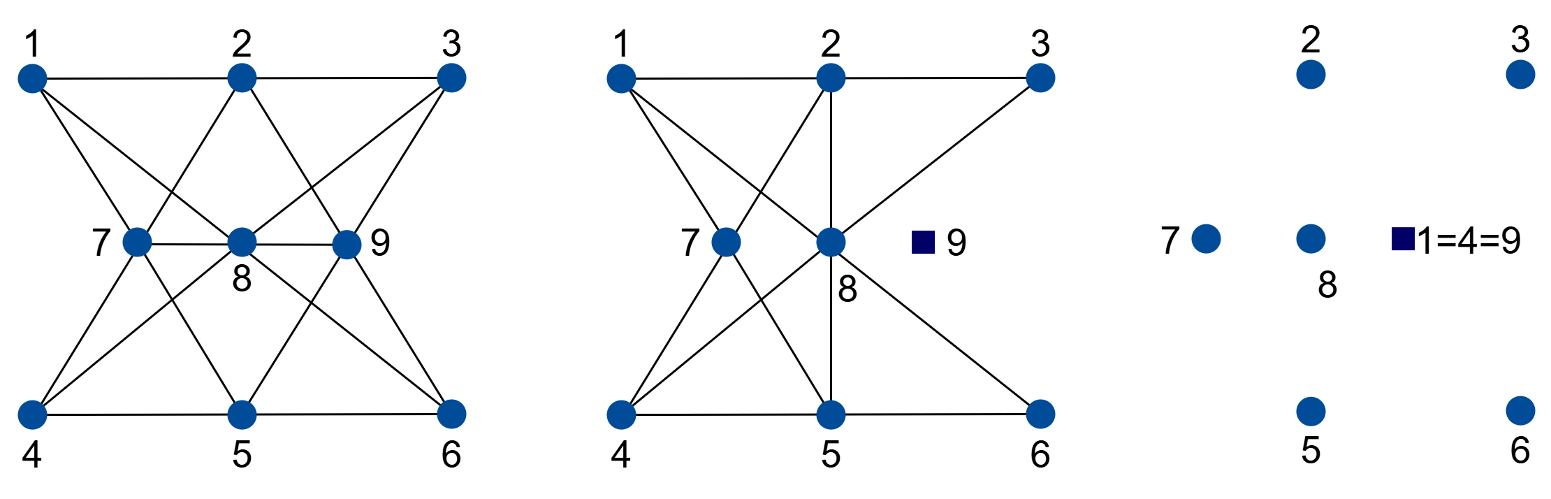
Figure 6: (Left) Pappus Configuration, (Center) $\displaystyle I_{9}$, (Right) $\displaystyle J_{1}$

In this work, we concentrate on addressing Questions 1.2 and 1.4 for three specific families of matroids of rank three: Cactus configurations, Pascal configuration, and Pappus configuration; see Definition 3.9, Figure 5 (b), and Figure 6 (Left). By applying Strategy 1, along with several additional techniques tailored to each case, we obtain the following main results:

Theorem (A).

The equality in (1.2) holds for the following matroids:

• Cactus configurations (Theorem 3.14)

• Pascal configuration (Theorem 4.14)

• Pappus configuration (Theorem 4.18)

Based on Theorem (A), one can derive explicit generating sets, up to radical, for the ideals corresponding to the Pascal and Pappus configurations. The table below summarizes the number of generators of each type: circuit polynomials, Grassmann–Cayley polynomials, and lifting polynomials. For detailed expressions and geometric interpretations of these generators, see Remarks 4.15 and 4.19.

Configuration	Circuit polynomials	Grassmann–Cayley polynomials	Lifting polynomials
Pascal	7	7	708,588
Pappus	9	9	2,361,960

The table highlights that the number of lifting polynomials in our generating sets is remarkably large, an observation that generally holds across configurations. This naturally leads to the question of whether smaller generating sets can be constructed. Although we do not pursue this direction in the present work, we pose the following as a guiding question for future research:

Question 1.5.

Develop efficient methods for constructing a minimal generating set for the ideal $\displaystyle I_{M}^{\textup{lift}}$.

Several previous works have provided complete sets of defining equations for specific families of matroids. In [21, 4, 17], it was shown that for certain families of configurations, the ideals $\displaystyle I_{\mathcal{C}(M)}$ and $\displaystyle I_{M}^{\text{lift}}$ suffice to generate the ideal $\displaystyle I_{M}$, up to radical. In [17, 3], other families were identified for which the ideals $\displaystyle I_{\mathcal{C}(M)}$ and $\displaystyle G_{M}$ generate $\displaystyle I_{M}$. To our knowledge, this is the first instance in which matroids are identified for which all three ideals $\displaystyle I_{\mathcal{C}(M)},I_{M}^{\text{lift}}$ and $\displaystyle G_{M}$ are needed to generate $\displaystyle I_{M}$.

In addition, we establish structural decomposition results for the matroid and circuit varieties associated with these configurations, namely Cactus, Pascal and Pappus configurations.

Theorem (B).

The following statements hold for cactus and Pascal configurations:

• Let $\displaystyle M$ be any cactus configuration. Then $\displaystyle M$ is realizable, and its matroid variety $\displaystyle V_{M}$ is irreducible. Moreover, if $\displaystyle Q_{M}$ denotes the set of points in $\displaystyle M$ that lie on at least three lines, the circuit variety $\displaystyle V_{\mathcal{C}(M)}$ has at most $\displaystyle 2^{\left|Q_{M}\right|}$ irredundant irreducible components, each obtained by setting a subset of points in $\displaystyle Q_{M}$ to be loops. (Theorems 3.9 and 3.16)

• The circuit variety of the Pascal configuration $\displaystyle N$ has the following irreducible decomposition:

  $$V_{\mathcal{C}(N)}=V_{N}\cup V_{U_{2,9}}\cup\bigcup_{i=7}^{9}V_{N(i)},$$

  where $\displaystyle U_{2,9}$ is the uniform matroid and $\displaystyle N(i)$ is obtained from $\displaystyle N$ by setting $\displaystyle i$ to be a loop.

Example 1.6.

Consider the cactus configuration shown in Figure 3 (Right), which determines a rank-three matroid $\displaystyle M$ on the ground set $\displaystyle[14]$. By Theorem (B), the matroid $\displaystyle M$ is realizable and the variety $\displaystyle V_{M}$ is irreducible. Moreover, since $\displaystyle Q_{M}=\{1,2,3\}$, the variety $\displaystyle V_{\mathcal{C}(M)}$ has at most eight irreducible components, each obtained by setting a subset of points in $\displaystyle\{1,2,3\}$ to be loops.

While the results presented herein may seem limited to particular families of matroids, it is important to note, as observed in [21], that determining a generating set for $\displaystyle I_{M}$ is notoriously difficult, with few general methods available for constructing such polynomials. The authors describe questions concerning the matroid ideal as having paved the road to Hell, descending into an abyss. The matroid ideals are only known for special classes of matroids. We hope that the ideas and techniques developed in this work will advance the understanding of matroid varieties and help identify the conditions under which Questions 1.2 and 1.4 have positive answers.

Before reviewing the contents of the paper we would like to comment on some related works. In [21], the authors developed an algorithm aimed at computing defining equations for the matroid variety associated with the $\displaystyle 3\times 4$ grid configuration, which contains 16 circuits of size three. Using Singular, they provided a finite generating set for the corresponding ideal. However, the computations stretch the capabilities of current computer algebra systems, and the resulting components lack a clear combinatorial interpretation. In [4], the authors obtained complete sets of defining equations for the matroid varieties of the quadrilateral set and the $\displaystyle 3\times 4$ grid, giving a geometric interpretation for such polynomials. In [17], the geometric liftability technique was used to define the ideal $\displaystyle I_{M}^{\textup{lift}}\subset I_{M}$. It was shown that, for paving matroids without points of degree greater than two, the ideal $\displaystyle I_{\mathcal{C}(M)}+I_{M}^{\textup{lift}}$ defines the associated matroid variety. In [24], the Grassmann–Cayley algebra was employed to define the ideal $\displaystyle G_{M}\subset I_{M}$. Using this approach, the authors constructed seven polynomials in the matroid ideal of Pascal configuration. In [17], it was shown that the ideal $\displaystyle I_{\mathcal{C}(M)}+G_{M}$ is equal to the associated matroid ideal of any forest configuration $\displaystyle M$, up to radical. For decomposing the circuit variety $\displaystyle V_{\mathcal{C}(M)}$, we adopt the algorithm introduced in [18, 19].

Although matroid varieties are widely studied in algebraic geometry for their intricate geometric structure, they also arise naturally in a range of other settings, including determinantal varieties [1, 3, 13, 21, 7], rigidity theory [15, 30, 10, 25], and conditional independence models [26, 6, 14, 5, 2]. In these contexts, one often encounters the problem of decomposing certain ideals such as conditional independence ideals or determinantal ideals into primary components. Notably, matroid ideals frequently appear as such primary components in such decompositions. As a result, understanding the defining equations of matroid varieties, or equivalently their associated matroid ideals, becomes essential for determining the primary decomposition of these broader classes of ideals.

We conclude the introduction with an outline of the paper. Section 2 reviews the necessary background on matroids and their associated varieties. In Section 3, we introduce and study cactus configurations. We prove that every such configuration corresponds to a nilpotent realizable matroid, and that its associated matroid variety is irreducible. Moreover, we determine a complete generating set, up to radical, for the matroid ideals of cactus configurations. Section 4 focuses on the Pascal and Pappus configurations, providing generating sets, up to radical, for their respective matroid ideals.

2 Preliminaries

This section provides a concise overview of properties of matroids and their associated varieties. For more details, we refer the reader to [20, 9, 22]. Throughout, we adopt the notation $\displaystyle[n]=\{1,\ldots,n\}$ and $\displaystyle\textstyle\binom{[d]}{n}$ to denote the set of $\displaystyle n$-element subsets of $\displaystyle[d]$.

2.1 Matroids

A matroid $\displaystyle M$ consists of a ground set $\displaystyle[d]$ together with a collection $\displaystyle\mathcal{I}$ of subsets of $\displaystyle[d]$, called independent sets, that satisfy the following three axioms: the empty set is independent, i.e., $\displaystyle\emptyset\in\mathcal{I}$; the hereditary property, meaning if $\displaystyle I\in\mathcal{I}$ and $\displaystyle I^{\prime}\subset I$, then $\displaystyle I^{\prime}\in\mathcal{I}$; and the exchange property, which states that if $\displaystyle I_{1},I_{2}\in\mathcal{I}$ with $\displaystyle|I_{1}|<|I_{2}|$, then there exists an element $\displaystyle e\in I_{2}\setminus I_{1}$ such that $\displaystyle I_{1}\cup\{e\}\in\mathcal{I}$.

The rank of $\displaystyle M$ is the size of its largest independent subset. Since we focus exclusively on matroids of rank at most three, all definitions will be stated in that context. Let $\displaystyle M$ be a matroid of rank three on the ground set $\displaystyle[d]$. We introduce the following notions:

• A subset of $\displaystyle[d]$ is called dependent if it is not independent. The collection of all dependent sets of $\displaystyle M$ is denoted by $\displaystyle\mathcal{D}(M)$.

• A subset of $\displaystyle[d]$ is called a circuit if it is a minimally dependent subset. The set of all circuits is denoted by $\displaystyle\mathcal{C}(M)$.

• A basis is an independent subset of $\displaystyle[d]$ of size three. The set of all bases is denoted by $\displaystyle\mathcal{B}(M)$.

• An element $\displaystyle x\in[d]$ is called a loop if $\displaystyle\{x\}\in\mathcal{C}(M)$.

• Two elements $\displaystyle x,y\in[d]$ are said to be parallel, or form a double point, if $\displaystyle\{x,y\}\in\mathcal{C}(M)$.

• $\displaystyle M$ is called simple if it contains no loops or parallel elements.

• The restriction of $\displaystyle M$ to $\displaystyle S$ is the matroid on $\displaystyle S$ whose independent sets are the independent sets of $\displaystyle M$ contained in $\displaystyle S$. The deletion of $\displaystyle S$, denoted $\displaystyle M\backslash S$, is defined as $\displaystyle M|([d]\backslash S)$.

• A line is defined as a maximal dependent subset of $\displaystyle[d]$, in which every subset of three elements is dependent. We denote the set of all lines of $\displaystyle M$ by $\displaystyle\mathcal{L}_{M}$, or simply $\displaystyle\mathcal{L}$ when the context is clear.

• Elements in $\displaystyle[d]$ are called points. For any point $\displaystyle p\in[d]$, let $\displaystyle\mathcal{L}_{p}$ denote the set of lines containing $\displaystyle p$. The degree of $\displaystyle p$ is defined as $\displaystyle\left|\mathcal{L}_{p}\right|$.

Example 2.1.

The uniform matroid $\displaystyle U_{2,d}$ on the ground set $\displaystyle[d]$ of rank $\displaystyle 2$ is defined as follows: each subset $\displaystyle S\subset[d]$ with $\displaystyle|S|\leq 2$ is independent, while those with $\displaystyle|S|>2$ are dependent.

Example 2.2.

Consider the configuration depicted in Figure 1 (Left). It defines a simple rank-three matroid on the ground set $\displaystyle[7]$, whose collection of lines is $\displaystyle\mathcal{L}=\{\{1,2,7\},\{3,4,7\},\{5,6,7\}\}$. The configuration in Figure 1 (Right) gives rise to a simple rank-three matroid on $\displaystyle[6]$, with set of lines $\displaystyle\{\{1,2,3\},\{1,5,6\},\{2,4,6\},\{3,4,5\}\}$. We refer to this matroid as the quadrilateral set, denoted by QS.

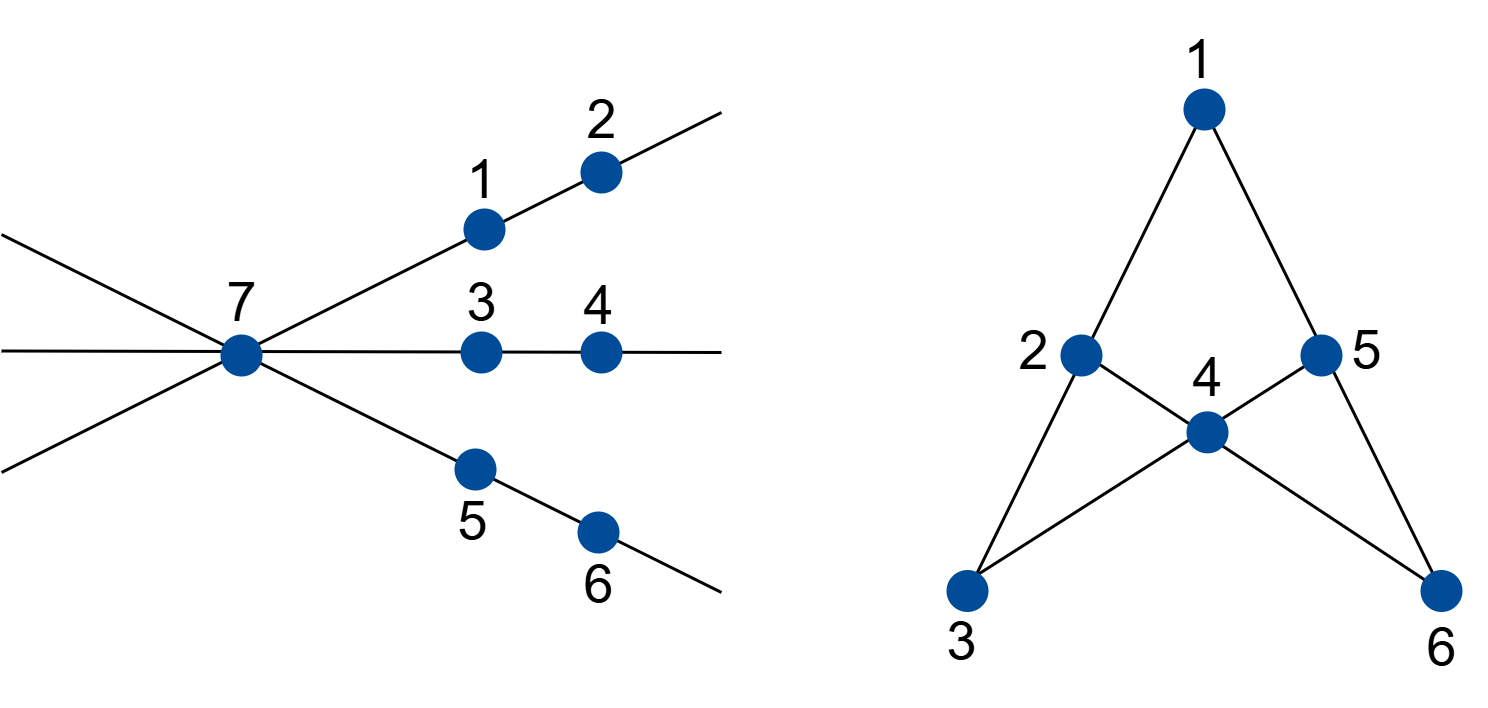
Figure 1: (Left) Three concurrent lines; (Right) Quadrilateral set.

As in the previous example, we will consistently identify each configuration with its associated rank-three matroid. We define two families of matroids that play a key role in this note; see [17].

Definition 2.3.

For a simple rank-three matroid $\displaystyle M$ on $\displaystyle[d]$, we define

$$S_{M}=\{p\in[d]:\left|\mathcal{L}_{p}\right|\geq 2\},\quad\text{and}\quad Q_{M}=\{p\in[d]:\left|\mathcal{L}_{p}\right|\geq 3\}.$$

We then consider the following chains of submatroids of $\displaystyle M$:

$$M_{0}=M,\ \quad M_{1}=M|S_{M},\quad\text{and }\quad M_{j+1}=M|S_{M_{j}}\quad\ \text{ for all $\displaystyle j\geq 1$.}$$

$$M^{0}=M,\quad M^{1}=M|Q_{M},\quad\text{and }\quad M^{j+1}=M|Q_{M^{j}}\quad\text{ for all $\displaystyle j\geq 1$.}$$

We say that $\displaystyle M$ is nilpotent if $\displaystyle M_{j}=\emptyset$ for some $\displaystyle j$, and solvable if $\displaystyle M^{j}=\emptyset$ for some $\displaystyle j$.

2.2 Matroid and circuit varieties

In this subsection, we describe several properties of the matroid and circuit varieties of a matroid $\displaystyle M$ of rank at most three, denoted $\displaystyle V_{M}$ and $\displaystyle V_{\mathcal{C}(M)}$, respectively. These varieties are defined in Definition 1.1.

Notation 2.4.

We fix the following notation that will be used throughout the paper.

1. For a $\displaystyle 3\times d$ matrix $\displaystyle X=\left(x_{i,j}\right)$ of indeterminates, we denote by $\displaystyle\mathbb{C}[X]$ the polynomial ring in the variables $\displaystyle x_{ij}$. Given subsets $\displaystyle A\subset[3]$ and $\displaystyle B\subset[d]$ with $\displaystyle\left|A\right|=\left|B\right|$, we denote by $\displaystyle[A|B]_{X}$ the minor of $\displaystyle X$ determined by the rows indexed by $\displaystyle A$ and columns indexed by $\displaystyle B$.

2. For vectors $\displaystyle v_{1},v_{2},v_{3}\subset\mathbb{C}^{3}$, we write $\displaystyle[v_{1},v_{2},v_{3}]$ for the determinant of the matrix whose columns are the vectors $\displaystyle v_{1},v_{2},v_{3}$.

3. To any matroid $\displaystyle M$ of rank at most three on $\displaystyle[d]$, we associate $\displaystyle X$, a $\displaystyle 3\times d$ matrix of indeterminates. For any subset $\displaystyle\{i_{1},\ldots,i_{k}\}\subset[d]$ with $\displaystyle k\leq 3$, and vectors $\displaystyle v_{1},\ldots,v_{3-k}\in\mathbb{C}^{3}$, we define

   $$[i_{1},\ldots,i_{k},v_{1},\ldots,v_{3-k}]\in\mathbb{C}[X],$$

   as the determinant of the $\displaystyle 3\times 3$ submatrix of $\displaystyle X$ whose columns are indexed by $\displaystyle i_{1},\ldots,i_{k}$ and $\displaystyle v_{1},\ldots,v_{3-k}$. Note that $\displaystyle[i_{1},\ldots,i_{k},v_{1},\ldots,v_{3-k}]$ is a polynomial in $\displaystyle\mathbb{C}[X]$, rather than a number.

The following introduces the circuit ideal $\displaystyle I_{\mathcal{C}(M)}$ and presents explicit equations that generate it.

Definition 2.5.

Let $\displaystyle M$ be a matroid of rank at most three on $\displaystyle[d]$. Consider the $\displaystyle 3\times d$ matrix $\displaystyle X=\left(x_{i,j}\right)$ of indeterminates. The circuit ideal, for which $\displaystyle V_{\mathcal{C}(M)}=V(I_{\mathcal{C}(M)})$, is defined as

$$I_{\mathcal{C}(M)}=\{[A|B]_{X}:\ B\in\mathcal{C}(M),\ A\subset[3],\ \text{and}\ |A|=|B|\}.$$

Remark 2.6.

Since $\displaystyle V_{M}\subset V_{\mathcal{C}(M)}$, we have $\displaystyle I_{\mathcal{C}(M)}\subset I_{M}$. Further, if $\displaystyle M$ is a simple rank-three matroid on $\displaystyle[d]$, then the ideal $\displaystyle I_{\mathcal{C}(M)}$ is generated by the following bracket polynomials defined in Notation 2.4(iii):

$$\{[i,j,k]:\{i,j,k\}\in\mathcal{C}(M)\}.$$

We recall the following result from [17], which will be used in the subsequent sections.

Theorem 2.7.

Let $\displaystyle M$ be a simple rank-three matroid on $\displaystyle[d]$.

• If $\displaystyle M$ is nilpotent and has no points of degree greater than two, then $\displaystyle V_{\mathcal{C}(M)}=V_{M}$.

• If $\displaystyle M$ is solvable, then $\displaystyle V_{M}$ is irreducible.

Since the Euclidean and Zariski closures of the realization space $\displaystyle\Gamma_{M}$ coincide, our general strategy to show that a collection of vectors $\displaystyle\gamma$ lies in $\displaystyle V_{M}$ is to demonstrate that an arbitrarily small perturbation of points can be applied to $\displaystyle\gamma$ to obtain an element in $\displaystyle\Gamma_{M}$. We formalize this in the following definition from [14], where a perturbation refers to a motion that can be made arbitrarily small. This concept will be used repeatedly throughout the paper.

Definition 2.8.

Let $\displaystyle\gamma\subset\mathbb{C}^{3}$ be a finite collection of vectors, and let $\displaystyle X$ denote a specific property. We say that a perturbation can be applied to $\displaystyle\gamma$ to obtain a new collection of vectors satisfying property $\displaystyle X$ if, for every $\displaystyle\epsilon>0$, it is possible to choose, for each vector $\displaystyle v\in\gamma$, a vector $\displaystyle\widetilde{v}$ such that $\displaystyle\lVert v-\widetilde{v}\rVert<\epsilon$, in such a way that the new collection satisfies property $\displaystyle X$.

When discussing a perturbation of a $\displaystyle k$-dimensional subspace $\displaystyle S\subset\mathbb{C}^{n}$, we consider $\displaystyle\{v_{1},\ldots,v_{k}\}$ a basis of it, and apply a perturbation to $\displaystyle\{v_{i}:i\in[k]\}$ to obtain another $\displaystyle k$-dimensional subspace.

2.3 Liftability

We now define liftable matroids. Throughout, let $\displaystyle M$ be a simple rank-three matroid on $\displaystyle[d]$.

Definition 2.9.

We introduce the following notions:

• Consider a collection of vectors $\displaystyle\gamma=\{\gamma_{i}:i\in[d]\}\subset\mathbb{C}^{3}$ and a vector $\displaystyle q\in\mathbb{C}^{3}$. We say that $\displaystyle\widetilde{\gamma}=\{\widetilde{\gamma}_{i}:i\in[d]\}\subset\mathbb{C}^{3}$ is a lifting of $\displaystyle\gamma$ from the vector $\displaystyle q$ if, for each $\displaystyle i\in[d]$, there exists $\displaystyle z_{i}\in\mathbb{C}$ such that $\displaystyle\widetilde{\gamma}_{i}=\gamma_{i}+z_{i}q$. Furthermore, we say that the lifting is non-degenerate if not all vectors of $\displaystyle\widetilde{\gamma}$ lie within the same hyperplane.

• The collection $\displaystyle\gamma$ is said to be liftable from the vector $\displaystyle q$, if the vectors $\displaystyle\gamma_{i}$ can be lifted from the point $\displaystyle q$ to a collection $\displaystyle\widetilde{\gamma}\in V_{\mathcal{C}(M)}$ with rank($\displaystyle\widetilde{\gamma})=3$.

• A simple rank-three matroid $\displaystyle M$ is liftable if, for any rank-two collection of vectors $\displaystyle\gamma=\{\gamma_{i}:i\in[d]\}$ in $\displaystyle\mathbb{C}^{3}$, there exists a non-degenerate lifting of $\displaystyle\gamma$ to a collection of vectors $\displaystyle\widetilde{\gamma}=\{\gamma_{i}+z_{i}q:i\in[d]\}\in V_{\mathcal{C}(M)}$, from any vector $\displaystyle q$ which is in general position with respect to $\displaystyle\gamma$.

In the next construction, we define the liftability matrix.

Definition 2.10.

Let $\displaystyle M$ be a simple rank-three matroid on $\displaystyle[d]$, and let $\displaystyle q\in\mathbb{C}^{3}$. We define the liftability matrix $\displaystyle\mathcal{M}_{q}(M)$ of $\displaystyle M$ and $\displaystyle q$, as the matrix with columns indexed by $\displaystyle[d]$ and rows indexed by the circuits of size three of $\displaystyle M$. The entries of this matrix are defined as follows: for each circuit $\displaystyle c=\{c_{1},c_{2},c_{3}\}\subset[d]$, the $\displaystyle c_{1}^{\text{th}},c_{2}^{\text{th}}$ and $\displaystyle c_{3}^{\text{th}}$ coordinate of the corresponding row are given by the polynomials

$$[c_{2},c_{3},q],\quad-[c_{1},c_{3},q],\quad\text{and}\quad[c_{1},c_{2},q],$$

where for the brackets we are using Notation 2.4(iii). The other entries of the row are set to $\displaystyle 0$. Note that the entries of the matrix are polynomials, not numbers. Given a collection of vectors $\displaystyle\gamma=\{\gamma_{1},\ldots,\gamma_{d}\}\subset\mathbb{C}^{3}$, we denote by $\displaystyle\mathcal{M}_{q}^{\gamma}(M)$ the matrix obtained from $\displaystyle\mathcal{M}_{q}(M)$ by substituting, for each $\displaystyle i\in[d]$, the three variables associated to index $\displaystyle i$ with the entries of $\displaystyle\gamma_{i}$.

Definition 2.11.

Consider a simple rank-three matroid $\displaystyle M$. We define the lifting ideal, denoted $\displaystyle I_{M}^{\text{lift}}$, as the ideal generated by all the $\displaystyle(|N|-2)$-minors of the liftability matrices $\displaystyle\mathcal{M}_{q}(N)$, where $\displaystyle N$ ranges over all full-rank submatroids of $\displaystyle M$ and $\displaystyle q$ varies over $\displaystyle\mathbb{C}^{3}$.

We recall some of the main properties of the lifting ideal; see Lemma 3.6 and Theorem 3.9 in [17].

Theorem 2.12.

Let $\displaystyle M$ be a simple rank-three matroid on $\displaystyle[d]$. Then $\displaystyle I_{M}^{\textup{lift}}\subseteq I_{M}$. Additionally, consider $\displaystyle\gamma=\{\gamma_{1},\ldots,\gamma_{d}\}\subset\mathbb{C}^{3}$, a collection of vectors in $\displaystyle V(I_{M}^{\text{lift}})$. Then $\displaystyle\gamma$ is liftable from any $\displaystyle q\in\mathbb{C}^{3}$, and such a lifting can be made arbitrarily small. The same holds for any full-rank submatroid of $\displaystyle M$.

2.4 Grassmann-Cayley algebra

We now review the notion of Grassmann-Cayley algebra from [28]. The Grassmann-Cayley algebra is the exterior algebra $\displaystyle\bigwedge(\mathbb{C}^{d})$, equipped with two operations: the join and the meet. The join, or extensor, of vectors $\displaystyle v_{1},\ldots,v_{k}$ is denoted by $\displaystyle v_{1}\cdots v_{k}$. The meet operation, denoted by $\displaystyle\wedge$, is defined for two extensors $\displaystyle v=v_{1}\cdots v_{k}$ and $\displaystyle w=w_{1}\cdots w_{j}$, with lengths $\displaystyle k$ and $\displaystyle j$ respectively, where $\displaystyle j+k\geq d$, as:

$$v\wedge w=\sum_{\sigma\in\mathcal{S}(k,j,d)}\left[v_{\sigma(1)}\ldots v_{\sigma(d-j)}w_{1}\ldots w_{j}\right]\cdot v_{\sigma(d-j+1)}\cdots v_{\sigma(k)}$$

where $\displaystyle\mathcal{S}(k,j,d)$ denotes the set of all permutations of $\displaystyle\left[k\right]$ that satisfy $\displaystyle\sigma(1)<\cdots<\sigma(d-j)$ and $\displaystyle\sigma(d-j+1)<\cdots<\sigma(d)$ and the bracket denotes the determinant, see Notation 2.4(ii). When $\displaystyle j+k<d$, the meet is defined as $\displaystyle 0$. There is a correspondence between the extensor $\displaystyle v=v_{1}\cdots v_{k}$ and the subspace $\displaystyle\overline{v}=\langle v_{1},\ldots,v_{k}\rangle$ that it generates. This correspondence satisfies the following properties:

Lemma 2.13.

Let $\displaystyle v=v_{1}\cdots v_{k}$ and $\displaystyle w=w_{1}\cdots w_{j}$ be two extensors with $\displaystyle j+k\geq d$. Then we have:

• The extensor $\displaystyle v$ is equal to zero if and only if the vectors $\displaystyle v_{1},\ldots,v_{k}$ are linear dependent.

• Any extensor $\displaystyle v$ is uniquely determined by $\displaystyle\overline{v}$ up to a scalar multiple.

• The meet of two extensors is again an extensor.

• We have that $\displaystyle v\wedge w\neq 0$ if and only if $\displaystyle\langle\overline{v},\overline{w}\rangle=\mathbb{C}^{d}$. In this case, we have $\displaystyle\overline{v}\cap\overline{w}=\overline{v\wedge w}.$

Example 2.14.

Consider the simple rank-three matroid depicted on Figure 5 (b). Since, in any realization, the lines $\displaystyle\{26,35,78\}$ are concurrent, the point of intersection of $\displaystyle 26$ and $\displaystyle 35$ lies on $\displaystyle 78$. Thus, the concurrency of the lines $\displaystyle\{26,35,78\}$ is equivalent to the vanishing of the following polynomial:

$$(26)\wedge(35)\vee 78=(\left[235\right]6-\left[635\right]2)\vee 78=\left[235\right]\left[678\right]-\left[635\right]\left[278\right].$$

Therefore, we know that this polynomial is contained in the ideal of the matroid variety.

2.4.1 Grassmann-Cayley ideal

We define the Grassmann-Cayley ideal using a construction outlined in [17]. Let $\displaystyle M$ be a simple rank-three matroid on $\displaystyle[d]$ and let $\displaystyle x\in[d]$. Consider distinct lines $\displaystyle l_{1}\neq l_{2}$ containing $\displaystyle x$ and points $\displaystyle p_{1},p_{2}\in l_{1}$, $\displaystyle p_{3},p_{4}\in l_{2}$. Let $\displaystyle P\in I_{M}$. Since $\displaystyle x=l_{1}\cap l_{2}$, for any realization $\displaystyle\gamma\in\Gamma_{M}$, we have:

$$\gamma_{x}=\gamma_{p_{1}}\gamma_{p_{2}}\wedge\gamma_{p_{3}}\gamma_{p_{4}}=\left[\gamma_{p_{1}},\gamma_{p_{2}},\gamma_{p_{3}}\right]\gamma_{p_{4}}-\left[\gamma_{p_{1}},\gamma_{p_{2}},\gamma_{p_{4}}\right]\gamma_{p_{3}}.$$

Consequently, the polynomial obtained from $\displaystyle P$ by replacing the variable $\displaystyle x$ with:

$$\left[p_{1},p_{2},p_{3}\right]p_{4}-\left[p_{1},p_{2},p_{4}\right]p_{3}$$

is also in $\displaystyle I_{M}$.

Definition 2.15.

Given a simple rank-three matroid $\displaystyle M$, the ideal $\displaystyle G_{M}$ is constructed as follows:

• Define the set $\displaystyle X_{0}$ as the polynomials generating the ideal $\displaystyle I_{\mathcal{C}(M)}$, i.e., the brackets corresponding to the circuits of size three of $\displaystyle M$, see Remark 2.6. For $\displaystyle j\geq 1$, recursively define the set $\displaystyle X_{j}$ as the polynomials obtained from those in $\displaystyle X_{j-1}$ by modifying some of their variables, potentially leaving them unchanged, according to the procedure described above. Note that $\displaystyle X_{0}\subset X_{1}\subset\ldots$.

• For $\displaystyle j\geq 0$, define the ideal $\displaystyle I_{j}$ as the ideal generated by the polynomials in $\displaystyle X_{j}$. Note that $\displaystyle I_{0}\subset I_{1}\subset\ldots$. Since the polynomial ring is Noetherian, this chain of ideals stabilizes. We denote the stabilized ideal by $\displaystyle G_{M}$.

We recall the following result from [17], which will be used repeatedly in the proofs that follow.

Proposition 2.16.

Let $\displaystyle M$ be a simple rank-three matroid on $\displaystyle[d]$. Then $\displaystyle G_{M}\subset I_{M}$. Moreover, let $\displaystyle l_{1},l_{2},l_{3}$ be lines of $\displaystyle M$ containing a common point $\displaystyle x\in[d]$. Then $\displaystyle\gamma_{l_{1}}\wedge\gamma_{l_{2}}\wedge\gamma_{l_{3}}=0$ for any $\displaystyle\gamma\in V_{\mathcal{C}(M)}\cap V(G_{M})$, meaning that the lines $\displaystyle\gamma_{l_{1}},\gamma_{l_{2}},\gamma_{l_{3}}$ are concurrent in $\displaystyle\mathbb{P}^{2}$. (If $\displaystyle\gamma_{x}=0$, one may redefine $\displaystyle\gamma_{x}$ to be the point in $\displaystyle\mathbb{P}^{2}$ contained in the intersection of the three lines $\displaystyle\gamma_{l_{1}},\gamma_{l_{2}}$ and $\displaystyle\gamma_{l_{3}}$).

3 Cactus configurations

In this section, we introduce cactus configurations and find a generating set for their associated matroid ideals, as well as the decomposition of their circuit varieties.

We begin by fixing the notation that will be used throughout this section. Throughout, we alternate freely between projective and affine language.

Notation 3.1.

Let $\displaystyle M$ be a simple matroid of rank three on $\displaystyle[d]$.

• For a collection of vectors $\displaystyle\gamma=\{\gamma_{1},\ldots,\gamma_{d}\}\in V_{\mathcal{C}(M)}$ and any line $\displaystyle l$ of $\displaystyle M$ we denote by $\displaystyle\gamma_{l}\subset\mathbb{C}^{3}$ the following two-dimensional subspace $\displaystyle\gamma_{l}=\operatorname{span}\{\gamma_{i}:i\in l\}$.

• The subspace $\displaystyle\gamma_{l}$ corresponds to a unique line in the projective plane $\displaystyle\mathbb{P}^{2}$, and we will therefore often refer to $\displaystyle\gamma_{l}$ simply as a line.

• Given that each nonzero vector $\displaystyle\gamma_{i}$ determines a point in $\displaystyle\mathbb{P}^{2}$, we use the terms vector and point interchangeably when $\displaystyle\gamma_{i}\neq 0$, depending on whether we are viewing it on $\displaystyle\mathbb{C}^{3}$ or $\displaystyle\mathbb{P}^{2}$.

• When two nonzero vectors $\displaystyle\gamma_{i}$ and $\displaystyle\gamma_{j}$ are linearly dependent, we may say they are the same point or that they coincide, denoted with $\displaystyle=$, reflecting that they are the same point in $\displaystyle\mathbb{P}^{2}$.

• If $\displaystyle\gamma_{i}=0$, we refer to $\displaystyle\gamma_{i}$ as a loop.

• Although it may seem natural to work entirely in the projective setting, the possible occurrence of zero vectors does not allow this simplification.

3.1 Irreducibility of matroid varieties of cactus configurations

In this subsection, we introduce the concept of cactus configurations and establish the irreducibility of their associated matroid varieties. We begin by introducing some necessary notions.

Definition 3.2.

Let $\displaystyle M$ be a simple matroid of rank at most three on $\displaystyle[d]$.

• If $\displaystyle M$ is the uniform matroid $\displaystyle U_{2,d}$, we refer to $\displaystyle M$ as a line; see Definition 2.1.

• Suppose $\displaystyle M$ has $\displaystyle n$ lines. We say that $\displaystyle M$ is a cycle if there exists a subset of points $\displaystyle\{p_{1},\ldots,p_{n}\}\subset[d]$ together with an ordering $\displaystyle\{l_{1},\ldots,l_{n}\}$ of its lines, such that:

  1. Each point $\displaystyle p_{i}$ is incident to precisely two lines, satisfying $\displaystyle\mathcal{L}_{p_{i}}=\{l_{i},l_{i+1}\}$, for each $\displaystyle i\in[n]$, where we identify $\displaystyle l_{n+1}$ with $\displaystyle l_{1}$.

  2. Every other point $\displaystyle p\in[d]\backslash\{p_{1},\ldots,p_{n}\}$ is incident to exactly one line, meaning $\displaystyle\left|\mathcal{L}_{p}\right|=1$.

Definition 3.3.

Let $\displaystyle M$ and $\displaystyle N$ be simple matroids of rank at most three on $\displaystyle[d_{1}]$ and $\displaystyle[d_{2}]$, respectively, and consider points $\displaystyle p\in[d_{1}]$ and $\displaystyle q\in[d_{2}]$. We define the free gluing of $\displaystyle M$ and $\displaystyle N$ at $\displaystyle p$ and $\displaystyle q$ as the simple rank-three matroid $\displaystyle M\amalg_{p,q}N$ on the ground set

$$([d_{1}]\backslash\{p\})\amalg([d_{2}]\backslash\{q\})\cup\{P\},$$

where $\displaystyle P$ is a new point that identifies both $\displaystyle p$ and $\displaystyle q$. The set of lines of $\displaystyle M\amalg_{p,q}N$ is given by:

$$\mathcal{L}_{M\amalg_{p,q}N}=\{(l\backslash\{p\})\cup\{P\}:l\in\mathcal{L}_{p}\}\cup\{(l\backslash\{q\})\cup\{P\}:l\in\mathcal{L}_{q}\}\cup(\mathcal{L}_{M}\backslash\mathcal{L}_{p})\cup(\mathcal{L}_{N}\backslash\mathcal{L}_{q}).$$

We now illustrate the above definition with two examples as follow.

Example 3.4.

Let $\displaystyle M$ denote the $\displaystyle 3\times 3$ grid configuration, and let $\displaystyle F$ be the Fano plane, as depicted in Figure 3. Figure 2 (Left) shows the free gluing $\displaystyle M\amalg_{7,7^{\prime}}F$ at the points $\displaystyle 7$ and $\displaystyle 7^{\prime}$.

Similarly, consider the configuration consisting of three concurrent lines and the quadrilateral set shown in Figure 1. Their free gluing along the points $\displaystyle 3$ and $\displaystyle 3^{\prime}$ is shown in Figure 2 (Right).

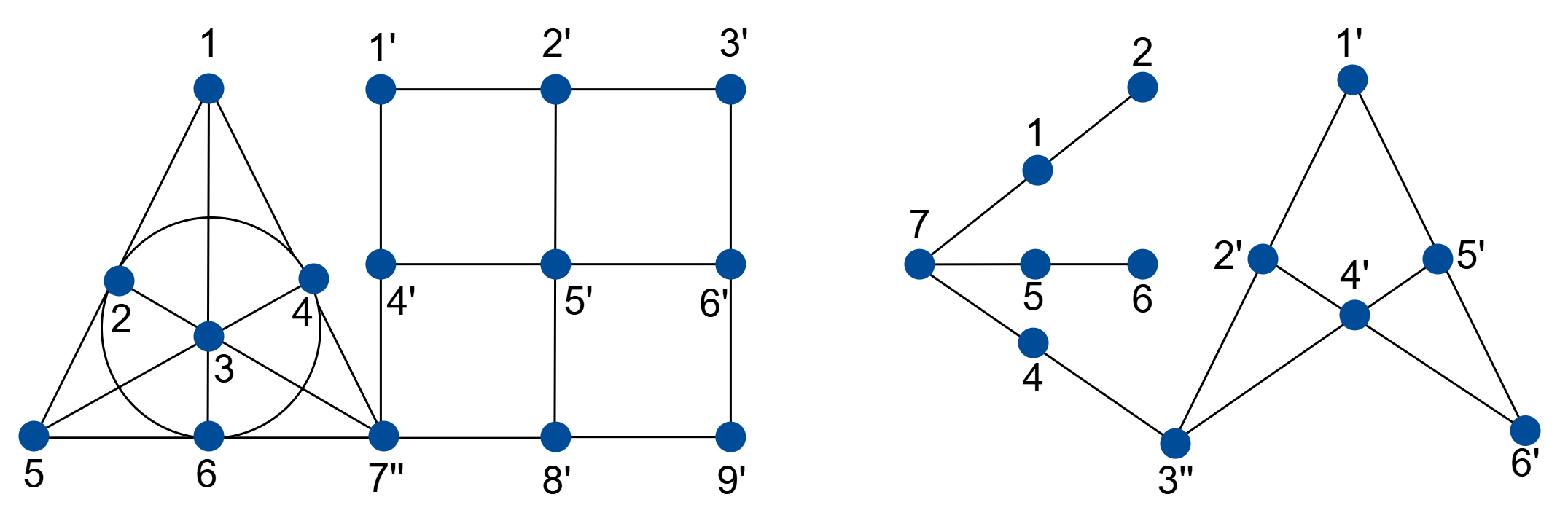
Figure 2: (Left) Free gluing of the Fano plane and the $\displaystyle 3\times 3$ grid; (Right) Free gluing of three concurrent lines and the quadrilateral set.

We can think of the free gluing $\displaystyle M\amalg_{p,q}N$ as the simple rank-three matroid obtained by gluing $\displaystyle M$ and $\displaystyle N$ at the points $\displaystyle p$ and $\displaystyle q$ in the most “free” or independent way, by preserving all dependencies of $\displaystyle M$ and $\displaystyle N$ without introducing any new ones. This notion of free gluing is closely related to the classical concept of amalgamation of matroids [23]. Given matroids $\displaystyle M$ and $\displaystyle N$ on ground sets $\displaystyle[d_{1}]$ and $\displaystyle[d_{2}]$, an amalgamation is a matroid whose restrictions to $\displaystyle[d_{1}]$ and $\displaystyle[d_{2}]$ agree with $\displaystyle M$ and $\displaystyle N$, respectively.

We are now prepared to define cactus configurations.

Definition 3.5.

A simple rank-three matroid $\displaystyle M$ is called a connected cactus configuration if it can be obtained by inductively freely gluing lines or cycles. More precisely, there exists a sequence of matroids $\displaystyle N_{1},\ldots,N_{k}$ such that:

• $\displaystyle N_{1}$ is either a line or a cycle.

• For each $\displaystyle i\in[k-1]$, $\displaystyle N_{i+1}$ is the free gluing of $\displaystyle N_{i}$ with a line or a cycle.

• $\displaystyle N_{k}=M$.

More generally, we say that a simple rank-three matroid is a cactus configuration if each of its connected components is a connected cactus configuration.

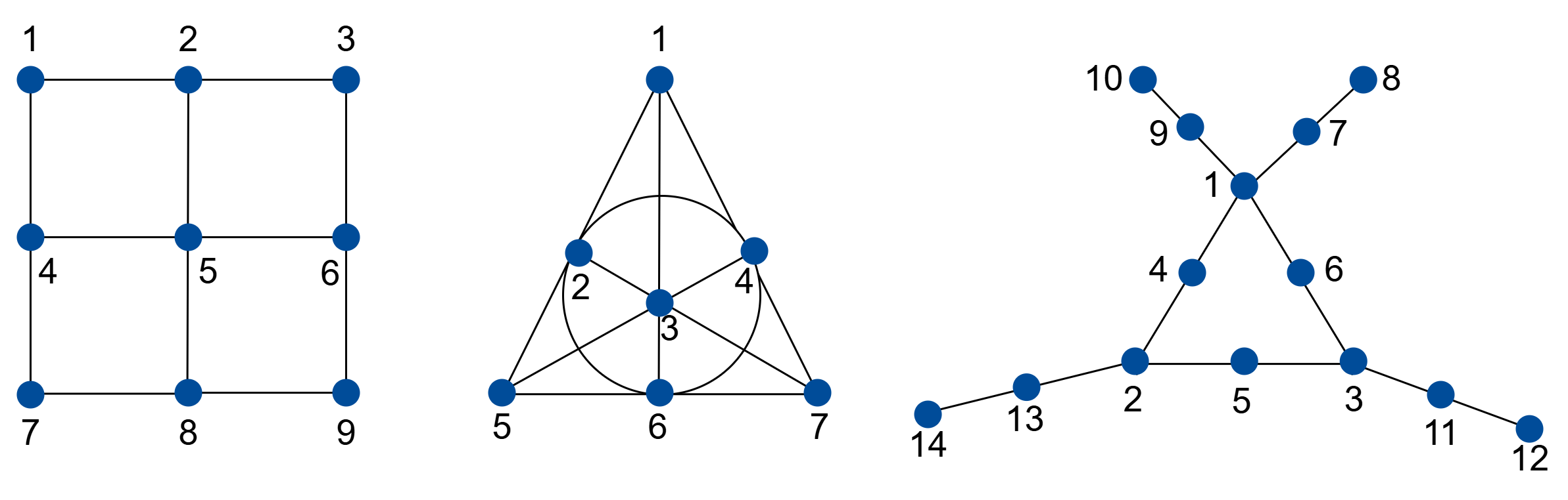
Figure 3: (Left) The $\displaystyle 3\times 3$ grid; (Center) Fano plane; (Right) Cactus configuration.

An example of a cactus configuration is shown in Figure 3 (Right). Our definition of cactus configurations is closely inspired by the notion of cactus graphs in graph theory. A cactus is a connected graph in which any two simple cycles share at most one vertex. Equivalently, it is a connected graph in which each edge is contained in at most one simple cycle. The following well-known property holds for cactus graphs.

Lemma 3.6.

Every cactus $\displaystyle G$ contains a subgraph $\displaystyle H$, which is either an edge or a cycle, such that at most one vertex of $\displaystyle H$ is adjacent to a vertex in $\displaystyle G\backslash H$.

We first provide an alternative characterization of cactus configurations in terms of cactus graphs.

Lemma 3.7.

To each simple matroid $\displaystyle M$ of rank at most three, we associate a simple graph $\displaystyle G(M)$ defined as follows:

• The vertices of $\displaystyle G(M)$ correspond to the points in $\displaystyle M$ of degree at least two.

• Two vertices of $\displaystyle G(M)$ are joined by an edge if and only if the corresponding points in $\displaystyle M$ lie on a common line.

Then $\displaystyle M$ is a cactus configuration if and only if $\displaystyle G(M)$ is a cactus graph.

Proof.

We may assume $\displaystyle M$ is connected, as the argument applies to each component separately.

First suppose that $\displaystyle G(M)$ is a cactus. We prove that $\displaystyle M$ is a cactus configuration by induction on the number of vertices of $\displaystyle G(M)$.

Base case: If $\displaystyle G(M)$ has only one vertex, then the statement is clear.

Inductive step: By Lemma 3.6, there exists a subgraph $\displaystyle H$, which is either an edge or a cycle, such that at most one of its vertices is adjacent to a vertex in $\displaystyle G(M)\backslash H$. Let $\displaystyle x$ denote this vertex. We then obtain that $\displaystyle M$ is of the form $\displaystyle M=M^{\prime}\amalg_{p,q}N$, where $\displaystyle G(M^{\prime})=H$, and $\displaystyle G(N)=(G(M)\backslash H)\cup\{x\}$, and the gluing is performed at the point corresponding to $\displaystyle\{x\}$. Since $\displaystyle H$ is an edge or a cycle in $\displaystyle G(M)$, $\displaystyle M^{\prime}$ is a line or a cycle configuration. Moreover, since $\displaystyle(G(M)\backslash H)\cup\{x\}$ is a cactus graph, the inductive hypothesis implies that $\displaystyle N$ is a cactus configuration. We thus conclude that $\displaystyle M$ is a cactus configuration.

Conversely, suppose that $\displaystyle M$ is a cactus configuration. By Definition 3.5, $\displaystyle M$ is constructed through a sequence of gluings of lines or cycles. We proceed by induction on the number $\displaystyle n$ of such gluings.

Base case: If $\displaystyle n=0$, then $\displaystyle M$ consists of a single line or cycle, in which case the statement is clear.

Inductive step: We know that $\displaystyle M$ is of the form $\displaystyle M=M^{\prime}\amalg_{p,q}N$, where $\displaystyle M^{\prime}$ is a line or a cycle and $\displaystyle N$ is a cactus configuration. Passing to the associated graphs, we see that $\displaystyle G(M^{\prime})$ and $\displaystyle G(N)$ are subgraphs of $\displaystyle G(M)$ sharing a unique vertex $\displaystyle x$ which corresponds to the point of gluing. Furthermore, $\displaystyle G(M^{\prime})$ is an edge or a cycle of $\displaystyle G(M)$ and $\displaystyle G(N)$ is a cactus graph by inductive hypothesis. Moreover, the gluing condition ensures that there is no edge in $\displaystyle G(M)$ connecting a vertex in $\displaystyle G(M^{\prime})\backslash\{x\}$ to a vertex in $\displaystyle G(N)\backslash\{x\}$. Hence, $\displaystyle G(M)$ is also a cactus graph, completing the proof. ∎

We next prove that every cactus configuration is nilpotent; recall Definition 2.3.

Proposition 3.8.

Every cactus configuration is nilpotent.

Proof.

Let $\displaystyle M$ be a cactus configuration. We may assume $\displaystyle M$ is connected, as the argument applies to each component separately. By Definition 3.5, $\displaystyle M$ is constructed through an iterative process of gluing lines or cycles. We establish the result by induction on the number $\displaystyle n$ of such gluings.

Base case: If $\displaystyle n=0$, then $\displaystyle M$ consists of a single line or cycle, in which case the statement is clear.

Induction step: Assume that the statement holds for any cactus configuration constructed from at most $\displaystyle n-1$ gluings, and consider a configuration $\displaystyle M$ obtained through $\displaystyle n$ gluings. At the $\displaystyle n^{\text{th}}$-step, $\displaystyle M$ takes the form $\displaystyle M=M^{\prime}\amalg_{p,q}N$, where $\displaystyle M^{\prime}$ is constructed from $\displaystyle n-1$ gluings, and $\displaystyle N$ is either a line or a cycle. Denote the ground sets of $\displaystyle M^{\prime}$ and $\displaystyle N$ by $\displaystyle[d_{1}]$ and $\displaystyle[d_{2}]$, respectively. The ground set of $\displaystyle M^{\prime}\amalg_{p,q}N$ is then given by $\displaystyle([d_{1}]\backslash p)\amalg([d_{2}]\backslash q)\cup\{P\}$, where $\displaystyle P$ is the point that identifies both $\displaystyle p$ and $\displaystyle q$.

Case 1. Suppose that $\displaystyle N$ is a line, or equivalently $\displaystyle N=U_{2,d_{2}}$. In this case, the points in $\displaystyle[d_{2}]\backslash P$ have degree one in $\displaystyle M^{\prime}\amalg_{p,q}N$, which implies that $\displaystyle S_{M}\subset M^{\prime}$ as a submatroid. By induction, $\displaystyle M^{\prime}$ is nilpotent, and since any submatroid of a nilpotent matroid is also nilpotent, it follows that $\displaystyle S_{M}$ is also nilpotent. Consequently, the nilpotent chain of $\displaystyle S_{M}$, as defined in Definition 2.3, eventually reaches the empty set, and the same must hold for $\displaystyle M$.

Case 2. Now assume that $\displaystyle N$ is a cycle. If $\displaystyle q$ has degree 2 in $\displaystyle N$, then for every line $\displaystyle l$ of $\displaystyle N$, we have $\displaystyle\left|S_{M}\cap l\right|=2$. Consequently, $\displaystyle S_{M}\cap[d_{2}]$ contains no lines, since a line must contain at least three points. This implies that $\displaystyle S_{S_{M}}\cap[d_{2}]\subset\{P\}$, and thus $\displaystyle S_{S_{M}}$ is a submatroid of $\displaystyle M^{\prime}$. The result then follows by applying the same argument as in the previous case. If $\displaystyle q$ has degree 1 in $\displaystyle N$, then there exists a line $\displaystyle l$ in $\displaystyle N$ for which $\displaystyle\left|S_{M}\cap l\right|=3$, and for all other lines $\displaystyle l\in\mathcal{L}_{N}$, $\displaystyle\left|S_{M}\cap l\right|=2$. Then, for each line $\displaystyle l$ of $\displaystyle N$, we have $\displaystyle\left|S_{S_{M}}\cap l\right|\leq 2$. Thus, $\displaystyle S_{S_{M}}\cap[d_{2}]$ contains no lines, and using the notation from Definition 2.3, we have $\displaystyle M_{3}\cap[d_{2}]\subset\{P\}$. The result again follows by applying the same argument as in the previous case. This completes the proof. ∎

We now prove the irreducibility of matroid varieties associated with cactus configurations.

Theorem 3.9.

Every cactus configuration $\displaystyle M$ is realizable, and its matroid variety $\displaystyle V_{M}$ is irreducible.

Proof.

By Proposition 3.8, $\displaystyle M$ is nilpotent, hence the result follows from [17, Theorem 4.12]. ∎

3.2 Matroid ideal of cactus configurations

In this subsection, we present a complete set of defining equations for the matroid varieties associated with cactus configurations, or equivalently, a finite generating set for their matroid ideals up to radical. To achieve this, we first establish a series of lemmas.

Definition 3.10.

Let $\displaystyle M$ be a matroid on $\displaystyle[d]$, and consider a subset $\displaystyle X\subset[d]$. We say that $\displaystyle X$ contains a cycle if there exist distinct points $\displaystyle x_{1},\ldots,x_{k}\in X$ and distinct lines $\displaystyle l_{1},\ldots,l_{k}$ of $\displaystyle M$ such that:

• $\displaystyle\{x_{i},x_{i+1}\}\subset l_{i}$ for every $\displaystyle i\in[k]$, where $\displaystyle x_{k+1}=x_{1}$.

Lemma 3.11.

Let $\displaystyle M$ be a simple rank-three matroid on $\displaystyle[d]$ and let $\displaystyle X\subset[d]$ be a subset of points that does not contain a cycle. Then, there exists a point $\displaystyle x\in X$ such that

$$|\{l\in\mathcal{L}_{x}:l\cap(X\backslash\{x\})\neq\emptyset\}|\leq 1.$$

Proof.

Suppose the contrary. Choose an arbitrary point $\displaystyle x_{1}\in X$. By assumption, there exists a line $\displaystyle l_{1}\in\mathcal{L}_{x_{1}}$ containing another point $\displaystyle x_{2}\in X$ with $\displaystyle x_{2}\neq x_{1}$. Applying the hypothesis again, we find a distinct line $\displaystyle l_{2}\neq l_{1}$ that contains $\displaystyle x_{2}$ and another point $\displaystyle x_{3}\neq x_{2}$. Repeating this process, we construct sequences of points $\displaystyle x_{1},x_{2},\ldots$ and lines $\displaystyle l_{1},l_{2},\ldots$ such that $\displaystyle x_{k}\neq x_{k+1}$, $\displaystyle l_{k}\neq l_{k+1}$, and $\displaystyle\{x_{k},x_{k+1}\}\subset l_{k}$. Since $\displaystyle X$ is finite, some point must eventually repeat, forming a cycle. This contradicts the assumption that $\displaystyle X$ does not contain a cycle, completing the proof. ∎

Recall from Definition 2.3 that $\displaystyle Q_{M}$ denotes the set of points in $\displaystyle M$ with degree at least three.

Lemma 3.12.

Let $\displaystyle M$ be a cactus configuration, and let $\displaystyle\gamma\in V_{\mathcal{C}(M)}$ with $\displaystyle\gamma_{p}\neq 0$ for all $\displaystyle p\in Q_{M}$. Then $\displaystyle\gamma$ can be perturbed to obtain a configuration $\displaystyle\tau\in\Gamma_{M}$.

Proof.

We may assume that $\displaystyle M$ is connected, since the argument can then be applied separately to each connected component. By Definition 3.5, $\displaystyle M$ is constructed through a sequence of gluings of lines or cycles. We prove the claim by induction on the number $\displaystyle m$ of such gluings.

Base case: If $\displaystyle m=0$, then $\displaystyle M$ is either a line or a cycle. By Theorem 2.7 (i), it follows that $\displaystyle V_{\mathcal{C}(M)}=V_{M}$, so we can perturb $\displaystyle\gamma$ to obtain $\displaystyle\tau\in\Gamma_{M}$.

Induction step: Assume that the statement holds for any cactus configuration constructed from at most $\displaystyle m-1$ gluings, and consider a cactus configuration $\displaystyle M$ obtained through $\displaystyle m$ gluings. At the $\displaystyle m^{\text{th}}$-step, $\displaystyle M$ takes the form $\displaystyle M=M^{\prime}\amalg_{p,q}N$, where $\displaystyle M^{\prime}$ is constructed from $\displaystyle m-1$ gluings, and $\displaystyle N$ is either a line or a cycle. Denote the ground sets of $\displaystyle M^{\prime}$ and $\displaystyle N$ by $\displaystyle[d_{1}]$ and $\displaystyle[d_{2}]$, respectively. The ground set of $\displaystyle M^{\prime}\amalg_{p,q}N$ is then $\displaystyle([d_{1}]\backslash p)\amalg([d_{2}]\backslash q)\cup\{P\}$, where $\displaystyle P$ is the point that identifies both $\displaystyle p$ and $\displaystyle q$.

We first show that we may assume $\displaystyle\gamma_{P}\neq 0$.

• If $\displaystyle P\in Q_{M}$, then $\displaystyle\gamma_{P}\neq 0$ by assumption.

• If $\displaystyle|\mathcal{L}_{P}|\leq 2$ and $\displaystyle\gamma_{P}=0$, consider the set $\displaystyle R=\{\gamma_{l}:l\in\mathcal{L}_{i}\textup{ and }\text{rk}(\gamma_{l})=2\}$. Since $\displaystyle i$ has degree at most two, we have $\displaystyle|R|\leq 2.$ If $\displaystyle|R|=0$, then perturb $\displaystyle\gamma$ arbitrarily away from the origin. If $\displaystyle|R|=1$, then perturb $\displaystyle\gamma$ on the unique line in $\displaystyle R$, away from the origin. If $\displaystyle|R|=2$, then perturb $\displaystyle\gamma$ on the intersection of the two distinct lines in $\displaystyle R$. In each case, the resulting configuration lies in $\displaystyle\Gamma_{M}$, as desired.

Case 1. Suppose that $\displaystyle N$ is a line. By the induction hypothesis, we can perturb the vectors $\displaystyle\{\gamma_{r}:r\in[d_{1}]\}$ to obtain a collection $\displaystyle\{\tau_{r}:r\in[d_{1}]\}$ in $\displaystyle\Gamma_{M^{\prime}}$. Since $\displaystyle\gamma_{P}\neq 0$, we can further extend $\displaystyle\tau$ to the points in $\displaystyle[d_{2}]\backslash\{q\}$ by applying a perturbation to the vectors $\displaystyle\{\gamma_{r}:r\in[d_{2}]\backslash q\}$, ensuring that these vectors remain on the same line as $\displaystyle\tau_{P}$ and on no other line. This yields a collection of vectors $\displaystyle\tau\in\Gamma_{M}$, as desired.

Case 2. Suppose that $\displaystyle N$ is a cycle. By the induction hypothesis, we can perturb the vectors $\displaystyle\{\gamma_{r}:r\in[d_{1}]\}$ to obtain a collection $\displaystyle\{\tau_{r}:r\in[d_{1}]\}$ in $\displaystyle\Gamma_{M^{\prime}}$. Similarly, as in the first case, we can perturb the vectors $\displaystyle\{\gamma_{r}:r\in[d_{2}]\}$ to obtain a collection $\displaystyle\{\beta_{r}:r\in[d_{2}]\}$ in $\displaystyle\Gamma_{N}$. Furthermore, since $\displaystyle\gamma_{p}\neq 0$, by applying a small rotation from the origin to the vectors in $\displaystyle\beta$, we can ensure that $\displaystyle\beta_{q}=\tau_{p}$. Next, we rotate $\displaystyle\beta$ infinitesimally around $\displaystyle\tau_{p}$ and observe that each $\displaystyle\beta_{r}\neq 0$ since $\displaystyle\beta\in\Gamma_{N}$. This guarantees that the vectors $\displaystyle\beta_{r}$ do not lie on any lines of the configuration other than those associated with $\displaystyle N$, for all $\displaystyle r\in[d_{2}]$. This yields a collection of vectors in $\displaystyle\Gamma_{M}$, as desired. ∎

Lemma 3.13.

Let $\displaystyle M$ be a cactus configuration, such that the points of $\displaystyle Q_{M}$ do not contain a cycle. If $\displaystyle\gamma\in V_{\mathcal{C}(M)}\cap V(G_{M})$, then there exists $\displaystyle\tau\in V_{\mathcal{C}(M)}$ such that:

• For every point $\displaystyle p\in Q_{M}$, we have $\displaystyle\tau_{p}\neq 0$.

In particular, $\displaystyle\tau$ can be chosen as a perturbation of $\displaystyle\gamma$.

Proof.

The proof follows by applying the same argument as in [17, Lemma 4.23]. ∎

We now establish the main result of this section.

Theorem 3.14.

Let $\displaystyle M$ be a cactus configuration, such that the points of $\displaystyle Q_{M}$ do not contain a cycle. Then $\displaystyle I_{M}=\sqrt{I_{\mathcal{C}(M)}+G_{M}}$.

Proof.

Denote by $\displaystyle I$ the ideal on the right-hand side, which is contained in $\displaystyle I_{M}$ by Proposition 2.16. To show the reverse inclusion, it suffices to show $\displaystyle V(I)\subseteq V_{M}$. Consider a collection of vectors $\displaystyle\gamma\in V_{\mathcal{C}(M)}\cap V(G_{M})$. By Lemma 3.13, we can perturb the vectors of $\displaystyle\gamma$ to a collection of vectors $\displaystyle\tau\in V_{\mathcal{C}(M)}$ such that $\displaystyle\tau_{p}\neq 0$ for all $\displaystyle p\in Q_{M}$. Applying Lemma 3.12, we obtain a collection of vectors $\displaystyle\tau^{\prime}\in\Gamma_{M}$ which is a perturbation of $\displaystyle\tau$. This proves that $\displaystyle\gamma\in V_{M}$, as desired. ∎

In the following example, we show that the acyclicity assumption on the points of $\displaystyle Q_{M}$ in Theorem 3.14 is essential and cannot be omitted.

Example 3.15.

Consider the matroid depicted in Figure 3 (Right), which we denote by $\displaystyle M$. Let

$$\gamma=\setcounter{MaxMatrixCols}{14}\begin{pmatrix}1&0&0&1&1&1&1&1&1&1&1&0&0&0\\ 0&1&0&1&2&4&5&6&7&9&8&0&0&0\\ 0&0&1&1&3&8&7&10&12&21&17&0&0&0\end{pmatrix},$$

where the columns correspond to the points $\displaystyle\{4,5,6,7,8,9,10,11,12,13,14,1,2,3\}$, respectively. Note that $\displaystyle\gamma\in V_{\mathcal{C}(M)}\cap V(G_{M})$. We will show that $\displaystyle\gamma\not\in V_{M}$.

Assume, for contradiction, that $\displaystyle\gamma\in V_{M}=\overline{\Gamma_{M}}$. Since the Zariski and Euclidean closures of $\displaystyle\Gamma_{M}$ coincide, it follows that for every $\displaystyle\epsilon>0$, we can choose an element $\displaystyle\gamma_{\epsilon}\in\Gamma_{M}$ such that $\displaystyle\lvert\gamma-\gamma_{\epsilon}\rvert<\epsilon$. After a perturbation, we may assume that $\displaystyle\gamma_{\epsilon}$ takes the form

$$\gamma_{\epsilon}=\setcounter{MaxMatrixCols}{14}\begin{pmatrix}1&0&0&1&1&1&1&1&1&1&1&x_{1}&x_{2}&x_{3}\\ 0&1&0&1&2+\epsilon(1)&4+\epsilon(3)&5+\epsilon(5)&6+\epsilon(7)&7+\epsilon(9)&9+\epsilon(11)&8+\epsilon(13)&y_{1}&y_{2}&y_{3}\\ 0&0&1&1&3+\epsilon(2)&8+\epsilon(4)&7+\epsilon(6)&10+\epsilon(8)&12+\epsilon(10)&21+\epsilon(12)&17+\epsilon(14)&z_{1}&z_{2}&z_{3}\end{pmatrix},$$

where the columns again correspond to $\displaystyle\{4,5,6,7,8,9,10,11,12,13,14,1,2,3\}$ and $\displaystyle\epsilon(i)\in\mathbb{C}$ satisfies $\displaystyle\lvert\epsilon(i)\rvert<\epsilon$ for all $\displaystyle i\in[14]$. Note that $\displaystyle\{1,9,10\}$ and $\displaystyle\{1,7,8\}$ are lines in $\displaystyle M$, hence the point $\displaystyle{\gamma_{\epsilon}}_{1}$ lies in the intersection of the lines spanned by $\displaystyle\{{\gamma_{\epsilon}}_{9},{\gamma_{\epsilon}}_{10}\}$ and $\displaystyle\{{\gamma_{\epsilon}}_{7},{\gamma_{\epsilon}}_{8}\}$. Therefore,

$${\gamma_{\epsilon}}_{1}={\gamma_{\epsilon}}_{9}{\gamma_{\epsilon}}_{10}\wedge{\gamma_{\epsilon}}_{7}{\gamma_{\epsilon}}_{8}.$$

Taking the limit $\displaystyle\epsilon\to 0$, we obtain $\displaystyle\lim_{\epsilon\to 0}{\gamma_{\epsilon}}_{1}=\gamma_{9}\gamma_{10}\wedge\gamma_{7}\gamma_{8}=(1,13/3,23/3)^{\top}$.

Similarly, $\displaystyle\{3,1,6\}$ and $\displaystyle\{3,11,12\}$ are lines of $\displaystyle M$, hence $\displaystyle{\gamma_{\epsilon}}_{3}$ lies in the intersection of the lines spanned by $\displaystyle\{{\gamma_{\epsilon}}_{1},{\gamma_{\epsilon}}_{6}\}$ and $\displaystyle\{{\gamma_{\epsilon}}_{11},{\gamma_{\epsilon}}_{12}\}$. Thus, $\displaystyle{\gamma_{\epsilon}}_{3}={\gamma_{\epsilon}}_{1}{\gamma_{\epsilon}}_{6}\wedge{\gamma_{\epsilon}}_{11}{\gamma_{\epsilon}}_{12}$. Taking the limit $\displaystyle\epsilon\to 0$, we obtain

$$\lim_{\epsilon\to 0}{\gamma_{\epsilon}}_{3}=\lim_{\epsilon\to 0}{\gamma_{\epsilon}}_{1}{\gamma_{\epsilon}}_{6}\wedge{\gamma_{\epsilon}}_{11}{\gamma_{\epsilon}}_{12}=(1,13/3,23/3)^{\top}\gamma_{6}\wedge\gamma_{11}\gamma_{12}=(1,13/3,20/3)^{\top}.$$

Similarly, $\displaystyle\{2,3,5\}$ and $\displaystyle\{2,13,14\}$ are lines of $\displaystyle M$. Thus, the triples of points $\displaystyle\{{\gamma_{\epsilon}}_{2},{\gamma_{\epsilon}}_{3},{\gamma_{\epsilon}}_{5}\}$ and $\displaystyle\{{\gamma_{\epsilon}}_{2},{\gamma_{\epsilon}}_{13},{\gamma_{\epsilon}}_{14}\}$ are collinear. Consequently, $\displaystyle{\gamma_{\epsilon}}_{2}={\gamma_{\epsilon}}_{3}{\gamma_{\epsilon}}_{5}\wedge{\gamma_{\epsilon}}_{13}{\gamma_{\epsilon}}_{14}$. Taking the limit $\displaystyle\epsilon\to 0$, we obtain

$$\lim_{\epsilon\to 0}{\gamma_{\epsilon}}_{2}=\lim_{\epsilon\to 0}{\gamma_{\epsilon}}_{3}{\gamma_{\epsilon}}_{5}\wedge{\gamma_{\epsilon}}_{13}{\gamma_{\epsilon}}_{14}=(1,13/3,20/3)^{\top}\gamma_{5}\wedge\gamma_{13}\gamma_{14}=(1,65/12,80/12)^{\top}.$$

Now, since $\displaystyle\{1,2,4\}$ is a line of $\displaystyle M$, and $\displaystyle\gamma_{\epsilon}\in\Gamma_{M}$, it must hold that $\displaystyle\det({\gamma_{\epsilon}}_{1},{\gamma_{\epsilon}}_{2},{\gamma_{\epsilon}}_{4})=0$. However, evaluating the limits give

$$\lim_{\epsilon\to 0}\det({\gamma_{\epsilon}}_{1},{\gamma_{\epsilon}}_{2},{\gamma_{\epsilon}}_{4}) =\det(\lim_{\epsilon\to 0}{\gamma_{\epsilon}}_{1},\lim_{\epsilon\to 0}{\gamma_{\epsilon}}_{2},\gamma_{4})$$

$$=\det((1,3/3,3/3)^{\top},(1,5/2,0/2)^{\top},\gamma_{4})$$

$$=-55\neq 0,$$

a contradiction. Thus $\displaystyle\gamma\notin V_{M}$, and so the acyclicity assumption in Theorem 3.14 is necessary.

3.3 Bound on the number of irreducible components of $\displaystyle V_{\mathcal{C}(M)}$

We now bound the number of irreducible components of the circuit variety of a cactus configuration.

Theorem 3.16.

Let $\displaystyle M$ be a cactus configuration. Then $\displaystyle V_{\mathcal{C}(M)}$ has at most $\displaystyle 2^{\lvert Q_{M}\rvert}$ irreducible components, each arising from setting a subset of $\displaystyle Q_{M}$ to be loops.

Proof.

Let $\displaystyle[d]$ be the ground set of $\displaystyle M$. For each subset $\displaystyle J\subset Q_{M}$, let $\displaystyle M(J)$ denote the matroid obtained from $\displaystyle M$ by setting the points of $\displaystyle J$ to be loops. We claim that the following equality holds:

$$V_{\mathcal{C}(M)}=\bigcup_{J\subset Q_{M}}V_{M(J)}.$$ (3.1)

The inclusion $\displaystyle\supset$ is clear since the matroids $\displaystyle M(J)$ have more dependencies than $\displaystyle M$. To establish the reverse inclusion, we must verify that every $\displaystyle\gamma\in V_{\mathcal{C}(M)}$ lies in the variety on the right-hand side of (3.1). To verify this, let us fix an arbitrary element $\displaystyle\gamma\in V_{\mathcal{C}(M)}$. Let $\displaystyle X$ be the set $\displaystyle\{x\in Q_{M}:\gamma_{x}=0\}$. The submatroid $\displaystyle M\backslash X$ is also a cactus configuration. Moreover, since $\displaystyle\gamma_{p}\neq 0$ for all $\displaystyle p\in[d]\backslash X$, it follows that $\displaystyle\gamma_{p}\neq 0$ for all $\displaystyle p\in Q_{M\backslash X}$. Therefore, by Lemma 3.12, we know that $\displaystyle{\left.\kern-1.2pt\gamma\vphantom{\small|}\right|_{[d]\backslash X}}\in V_{M\backslash X}$, which implies that $\displaystyle\gamma\in V_{M(X)}$. This proves the claim.

By Theorem 3.9, each variety on the right-hand side of (3.1) is irreducible. It follows that $\displaystyle V_{\mathcal{C}(M)}$ has at most $\displaystyle 2^{\left|Q_{M}\right|}$ irreducible components. ∎

4 Pascal and Pappus configurations

In this section, we determine a finite generating set, up to radical, for the matroid ideals of the Pascal and Pappus configurations.

4.1 A sufficient criterion for liftability

The main result of this subsection is Proposition 4.8, which establishes a sufficient condition for an affirmative answer to the following question:

Question 4.1.

Let $\displaystyle M$ be a simple rank-three matroid on $\displaystyle[d]$ and suppose $\displaystyle\{\gamma_{1},\ldots,\gamma_{d-1}\}\subset\mathbb{P}^{2}$ is a collection of points lying on a common line $\displaystyle l\subset\mathbb{P}^{2}$ which is liftable from a point $\displaystyle q\in\mathbb{P}^{2}$ to a collection in $\displaystyle V_{\mathcal{C}(M\backslash d)}$. Does there exist a point $\displaystyle\gamma_{d}\in l$ such that the extended collection $\displaystyle\{\gamma_{1},\ldots,\gamma_{d}\}$ is liftable from $\displaystyle q$ to a collection in $\displaystyle V_{\mathcal{C}(M)}$?

In the following sections, we will apply Proposition 4.8 to compute the matroid ideals associated with the Pascal and Pappus configurations. In the context of the preceding question and throughout this subsection, a lifting always refers to a non-degenerate one, that is, a lifting in which the resulting vectors span the entire space. We begin by introducing a definition.

Definition 4.2.

Let $\displaystyle M$ be a simple rank-three matroid on $\displaystyle[d]$ and let $\displaystyle\gamma$ be a collection of vectors in $\displaystyle V_{\mathcal{C}(M)}$ and $\displaystyle q\in\mathbb{C}^{3}$ a vector in general position with respect to $\displaystyle\gamma$. Following Definition 2.9, we denote by $\displaystyle\textup{Lift}_{M,q}(\gamma)\subset\mathbb{C}^{d}$ the subspace composed of all vectors $\displaystyle(z_{1},\ldots,z_{d})$ such that the collection of vectors given by $\displaystyle\widetilde{\gamma}_{i}=\gamma_{i}+z_{i}q$ belongs to $\displaystyle V_{\mathcal{C}(M)}$. We also denote

$$\operatorname{dim}_{q}^{\gamma}(M)=\operatorname{dim}(\textup{Lift}_{M,q}(\gamma)),$$

the dimension of the space of liftings of $\displaystyle\gamma$. By [17, Lemma 4.31], this number equals $\displaystyle\operatorname{dim}(\ker(\mathcal{M}_{q}^{\gamma}(M)))$, where $\displaystyle\mathcal{M}_{q}^{\gamma}(M)$ is the matrix defined in Definition 2.10. For any submatroid $\displaystyle M|S$, we denote by $\displaystyle\operatorname{dim}_{q}^{\gamma}(M|S)$ the dimension $\displaystyle\operatorname{dim}_{q}^{\gamma}(M|S):=\operatorname{dim}\big{(}\textup{Lift}_{M|S,q}({\left.\kern-1.2pt\gamma\vphantom{\small|}\right|_{S}})\big{)}$.

We now show that, under an additional natural assumption, the quantity $\displaystyle\operatorname{dim}_{q}^{\gamma}(M)$ is independent of the choice of $\displaystyle q$ and $\displaystyle\gamma$ for nilpotent matroids. Before that we introduce some notation.

Notation 4.3.

Let $\displaystyle M$ be a matroid on $\displaystyle[d]$ and let $\displaystyle w=(p_{1},\ldots,p_{d})$ be an ordering of its elements. We denote by $\displaystyle M_{w,i}$ the restriction $\displaystyle M\mid\{p_{1},\ldots,p_{i}\}$, and we define $\displaystyle w_{i}$ to be the degree of $\displaystyle p_{i}$ in $\displaystyle M_{w,i}$. Note that if $\displaystyle M$ is nilpotent, then there exists an ordering $\displaystyle w$ for which

$$\text{max}\{w_{i}:i\in[d]\}\leq 1.$$ (4.1)

Theorem 4.4.

Let $\displaystyle M$ be a nilpotent matroid on $\displaystyle[d]$ and let $\displaystyle w=(i_{1},\ldots,i_{d})$ be an ordering of its points satisfying condition (4.1). Then, for any $\displaystyle\gamma\in V_{\mathcal{C}(M)}$ with no coinciding points or loops, and for any $\displaystyle q\in\mathbb{C}^{3}$ in general position with respect to $\displaystyle\gamma$, we have

$$\operatorname{dim}_{q}^{\gamma}(M)=d-\sum_{i=1}^{d}w_{i}.$$ (4.2)

Proof.

We proceed by induction on $\displaystyle d$, the size of the ground set. The base case $\displaystyle d=3$ is immediate.

For the inductive step, assume the result holds for all nilpotent matroids with at most $\displaystyle d-1$ elements. Let $\displaystyle M$ be a nilpotent matroid on $\displaystyle[d]$, and consider an arbitrary collection of vectors $\displaystyle\gamma\in V_{\mathcal{C}(M)}$ with no coinciding points or loops. Let $\displaystyle q\in\mathbb{C}^{3}$ be in general position with respect to $\displaystyle\gamma$. Our goal is to establish (4.2). Let $\displaystyle\gamma^{\prime}$ be the restriction of $\displaystyle\gamma$ to $\displaystyle\{p_{1},\ldots,p_{d-1}\}$. By the inductive hypothesis, we have

$$\operatorname{dim}_{q}^{\gamma^{\prime}}(M_{w,d-1})=d-1-\sum_{i=1}^{d-1}w_{i}.$$ (4.3)

We consider two cases based on the value of $\displaystyle w_{d}=\deg(p_{d})$.

Case 1. Suppose that $\displaystyle\deg(p_{d})=0$. In this case, the point $\displaystyle p_{d}$ does not belong to any circuit of size three in $\displaystyle M$. Therefore, any lifting of the vectors in $\displaystyle\gamma$ is completely determined by a lifting of the vectors in $\displaystyle\gamma^{\prime}$, together with an arbitrary lifting of the vector $\displaystyle\gamma_{p_{d}}$. Hence, $\displaystyle\operatorname{dim}_{q}^{\gamma}(M)=\operatorname{dim}_{q}^{\gamma^{\prime}}(M_{w,d-1})+1$. Substituting Equation (4.3), we obtain Equation (4.2), as desired.

Case 2. Suppose that $\displaystyle\deg(p_{d})=1$. Then $\displaystyle p_{d}$ lies on a unique line $\displaystyle l$ of $\displaystyle M$. Any lifting of the vectors $\displaystyle\gamma$ is thus determined by a lifting of the vectors $\displaystyle\gamma^{\prime}$, together with a unique scalar $\displaystyle z_{p_{d}}$ such that the lifted vector $\displaystyle\gamma_{p_{d}}+z_{p_{d}}q$ belongs to the two-dimensional subspace $\displaystyle\mathrm{span}\{\gamma_{i}:i\in l\setminus\{p_{d}\}\}$. This subspace is two-dimensional because $\displaystyle\gamma\in V_{\mathcal{C}(M)}$ has no coinciding points, and the uniqueness of $\displaystyle z_{p_{d}}$ follows from the assumption that $\displaystyle\gamma$ has no loops. Therefore, the contribution from $\displaystyle p_{d}$ does not increase the dimension, and we have $\displaystyle\operatorname{dim}_{q}^{\gamma}(M)=\operatorname{dim}_{q}^{\gamma^{\prime}}(M_{w,d-1})$. Applying Equation (4.3) again yields Equation (4.2). ∎

Definition 4.5.

For a nilpotent matroid $\displaystyle M$, we denote by $\displaystyle\operatorname{dim}(M)$ the number from Equation (4.2).

The next proposition provides an affirmative answer to Question 4.1 in the case where the degree of the point $\displaystyle d$ is at most two.

Proposition 4.6.

Let $\displaystyle M$ be a simple rank-three matroid on $\displaystyle[d]$ and suppose $\displaystyle\{\gamma_{1},\ldots,\gamma_{d-1}\}\subset\mathbb{P}^{2}$ is a collection of points lying on a common line $\displaystyle l\subset\mathbb{P}^{2}$ which is liftable from a point $\displaystyle q\in\mathbb{P}^{2}$ to a collection in $\displaystyle V_{\mathcal{C}(M\backslash d)}$. Moreover, assume that $\displaystyle\deg(d)\leq 2$. Then, there exists a point $\displaystyle\gamma_{d}\in l$ such that the extended collection $\displaystyle\{\gamma_{1},\ldots,\gamma_{d}\}$ is liftable from $\displaystyle q$ to a collection in $\displaystyle V_{\mathcal{C}(M)}$.

Proof.

We divide the proof into cases depending on the degree of $\displaystyle d$.

Case 1. Suppose that $\displaystyle\deg(d)=0$. In this case, we can extend $\displaystyle\gamma$ by selecting an arbitrary point $\displaystyle\gamma_{d}\in l$. The resulting collection is liftable from $\displaystyle q$ since any lifting of $\displaystyle\{\gamma_{1},\ldots,\gamma_{d-1}\}$ to a collection in $\displaystyle V_{\mathcal{C}(M\backslash\{d\})}$ and an arbitrary lifting of the point $\displaystyle\gamma_{d}$ represents a lifting to a collection in $\displaystyle V_{\mathcal{C}(M)}$.

Case 2. Suppose that $\displaystyle\deg(d)=1$ and let $\displaystyle l$ be the unique line of $\displaystyle M$ to which it belongs. In this case, again any arbitrary point $\displaystyle\gamma_{d}\in l$ results in a collection which is liftable from $\displaystyle q$. To see this, consider the lifting of the points $\displaystyle\{\gamma_{1},\ldots,\gamma_{d-1}\}$ from $\displaystyle q$ to a collection $\displaystyle\widetilde{\gamma}$ in $\displaystyle V_{\mathcal{C}(M\backslash d)}$ and lift the point $\displaystyle\gamma_{d}$ from $\displaystyle q$ to a point in $\displaystyle\widetilde{\gamma}_{l}$ resulting in a non-degenerate collection in $\displaystyle V_{\mathcal{C}(M)}$.

Case 3. Suppose that $\displaystyle\deg(p)=2$ and let $\displaystyle l_{1}$ and $\displaystyle l_{2}$ be the lines of $\displaystyle M$ containing $\displaystyle d$. In this case, if $\displaystyle\widetilde{\gamma}\in V_{\mathcal{C}(M\backslash d)}$ is a lifting of the points $\displaystyle\{\gamma_{1},\ldots,\gamma_{d-1}\}$ from $\displaystyle q$, extending $\displaystyle\gamma$ by setting $\displaystyle\gamma_{d}$ as the projection of $\displaystyle\widetilde{\gamma}_{l_{1}}\cap\widetilde{\gamma}_{l_{2}}$ from $\displaystyle q$ on $\displaystyle l$ works by applying the same argument as in Case 2. ∎

The preceding proposition essentially establishes that if $\displaystyle\deg(d)\leq 2$, then Question 4.1 has a positive answer. We now provide a sufficient condition for obtaining a positive answer when $\displaystyle\deg(d)\geq 3$. Before introducing the final property of this section, we recall a classical result from algebraic geometry, stated as Proposition I.7.1 in [12].

Proposition 4.7.

Let $\displaystyle Y\subset\mathbb{C}^{n}$ and $\displaystyle Z\subset\mathbb{C}^{n}$ be varieties of dimensions $\displaystyle r$ and $\displaystyle s$, respectively. Then every irreducible component of $\displaystyle Y\cap Z$ has dimension at least $\displaystyle r+s-n.$

We now prove the main result of this subsection, which will be fundamental in what follows.

Proposition 4.8.

Let $\displaystyle M$ be a simple rank-three matroid on $\displaystyle[d]$. Then, within the framework of Question 4.1, the answer is affirmative under the following assumptions:

1. $\displaystyle M\backslash\{d\}$ is nilpotent and satisfies $\displaystyle\operatorname{dim}(M\backslash\{d\})\geq 1+\deg(d).$

2. $\displaystyle\gamma$ has no coinciding points.

Proof.

Let $\displaystyle\mathcal{L}_{d}$ denote the set of lines of $\displaystyle M$ containing the point $\displaystyle d$. We will first prove that there exists a vector $\displaystyle z=(z_{1},\ldots,z_{d})$ such that the lifting $\displaystyle\tau_{z}=\{\gamma_{1}+z_{1}q,\ldots,\gamma_{d-1}+z_{d-1}q\}$ of the points $\displaystyle\{\gamma_{1},\ldots,\gamma_{d-1}\}$ satisfies the following conditions:

1. $\displaystyle\tau_{z}\in V_{\mathcal{C}(M\backslash\{d\})}$.

2. The lines $\displaystyle\{(\tau_{z})_{l}:l\in\mathcal{L}_{d}\}$ are concurrent.

3. $\displaystyle\tau_{z}$ is non degenerate.

We define two varieties $\displaystyle Y,Z\subset\mathbb{C}^{d}$ as follows:

$$Y=\{z\in\mathbb{C}^{d}:\tau_{z}\in V_{\mathcal{C}(M\backslash\{d\})}\},\quad\text{and}\quad Z=\{z\in\mathbb{C}^{d}:\text{the lines $\displaystyle\{(\tau_{z})_{l}:l\in\mathcal{L}_{d}\}$ are concurrent}\}.$$

By definition, $\displaystyle Y$ is precisely the linear space $\displaystyle\textup{Lift}_{M\backslash\{d\},q}(\gamma)$ introduced in Definition 4.2, and thus

$$\operatorname{dim}(Y)=\operatorname{dim}_{q}^{\gamma}(M\backslash\{d\})=\operatorname{dim}(M\backslash\{d\}),$$

where the final equality follows from Theorem 4.4.

To describe $\displaystyle Z$, let $\displaystyle\{l_{1},\ldots,l_{\deg(d)}\}$ be the lines in $\displaystyle\mathcal{L}_{d}$, and for each $\displaystyle l_{i}$, choose two distinct points $\displaystyle p_{i_{1}}$ and $\displaystyle p_{i_{2}}$ on $\displaystyle l_{i}$. Then, $\displaystyle Z$ consists of those $\displaystyle z\in\mathbb{C}^{d}$ for which the following families of lines are concurrent:

$$\begin{array}[]{ll}\{(\tau_{z})_{l_{1}},(\tau_{z})_{l_{2}},(\tau_{z})_{l_{3}}\},\ldots,\{(\tau_{z})_{l_{1}},(\tau_{z})_{l_{2}},(\tau_{z})_{l_{\deg(d)}}\}.\end{array}$$

Using the Grassmann-Cayley algebra, we have that the concurrency of these $\displaystyle\text{deg}(d)-2$ triples of lines can be translated as the vanishing of the following $\displaystyle\text{deg}(d)-2$ polynomials:

$$((\tau_{z})_{p_{1_{1}}}\vee(\tau_{z})_{p_{1_{2}}})\wedge((\tau_{z})_{p_{2_{1}}}\vee(\tau_{z})_{p_{2_{2}}})\vee((\tau_{z})_{p_{j_{1}}}\vee(\tau_{z})_{p_{j_{2}}}),$$

for $\displaystyle 3\leq j\leq d$. Since $\displaystyle Z$ is given by the vanishing locus of $\displaystyle\deg(d)-2$ polynomials, we have $\displaystyle\operatorname{dim}(Z)\geq d+2-\deg(d)$. Note that $\displaystyle 0\in Y\cap Z$, so $\displaystyle Y\cap Z$ is nonempty. By Proposition 4.7,

$$\operatorname{dim}(Y\cap Z)\geq\operatorname{dim}(Y)+\operatorname{dim}(Z)-d\geq\operatorname{dim}(M\backslash\{d\})+2-\deg(d).$$

Since $\displaystyle\operatorname{dim}(M\backslash\{d\})\geq\deg(d)+1$ by hypothesis, it follows that $\displaystyle\operatorname{dim}(Y\cap Z)\geq 3$. Since the space of trivial liftings of $\displaystyle\gamma$, corresponding to degenerate liftings, has dimension two, we then conclude that there exists $\displaystyle z\in Y\cap Z$ such that $\displaystyle\tau_{z}$ is non-degenerate. This lifting satisfies all the desired conditions.

Finally, let $\displaystyle x$ be the unique point of intersection of the lines $\displaystyle\{(\tau_{z})_{l}:l\in\mathcal{L}_{d}\}$. We define $\displaystyle\gamma_{d}$ as the projection of $\displaystyle x$ from $\displaystyle q$ onto the line $\displaystyle l$. This yields a liftable collection with respect to $\displaystyle M$ and $\displaystyle q$. ∎

4.2 Pascal Configuration

In this section, we study the Pascal configuration, the simple rank-three matroid in Figure 5(b). Specifically, we determine the irreducible decomposition of its circuit variety and find a finite generating set for its matroid ideal, up to radical. Throughout this subsection, we denote this matroid by $\displaystyle M$.

4.2.1 Irreducible decomposition of $\displaystyle V_{\mathcal{C}(M)}$

We introduce the following notation for the remainder of the paper:

Notation 4.9.

For a matroid $\displaystyle N$ of rank at most three on $\displaystyle[d]$, we define:

• $\displaystyle\pi_{N}^{i}$ as the matroid on $\displaystyle[d]$ in which all points, except for $\displaystyle i$, lie on a single line. Moreover, points that share a common line with $\displaystyle i$ in $\displaystyle N$ are identified. See Figure 5 (a) for an illustration of $\displaystyle\pi_{M}^{1}$.

• $\displaystyle N(i)$ denotes the matroid obtained by making $\displaystyle i$ a loop. More generally, for a subset $\displaystyle\{i_{1},\ldots,i_{k}\}\subset[d]$, we define $\displaystyle N(i_{1},i_{2},\ldots,i_{k})$ as the matroid obtained by turning all points in $\displaystyle\{i_{1},i_{2},\ldots,i_{k}\}$ into loops. This matroid is isomorphic to $\displaystyle N\backslash\{i_{1},\ldots,i_{k}\}$ up to removal of loops.

• Given a collection of vectors $\displaystyle\{\gamma_{1},\ldots,\gamma_{d}\}\subset\mathbb{C}^{3}$ and a subset $\displaystyle A\subset[d]$, we denote by $\displaystyle\gamma_{A}\subset\mathbb{C}^{3}$ the linear span of the vectors $\displaystyle\{\gamma_{a}:a\in A\}$.

Moreover, the following remark will be used throughout the remainder of the paper.

Remark 4.10.

For any given configuration, there exists a sufficiently small perturbation that does not introduce new dependencies. Throughout, we assume that all perturbations satisfy this condition.

The following lemmas plays a key role in our discussion. Recall that for a matroid $\displaystyle N$, we denote by $\displaystyle N(i)$ the matroid obtained from $\displaystyle N$ by declaring $\displaystyle i$ to be a loop.

Lemma 4.11.

Let $\displaystyle M$ be a simple rank-three matroid on $\displaystyle[d]$ and assume that the point $\displaystyle i\in[d]$ has degree at most two. Then $\displaystyle V_{M(i)}\subseteq V_{M}$.

Proof.

We show that any collection $\displaystyle\gamma\in\Gamma_{M(i)}$ can be perturbed to a collection in $\displaystyle\Gamma_{M}$, hence $\displaystyle\gamma\in V_{M}$. Let $\displaystyle\gamma\in V_{\mathcal{C}(M)}$, and consider the set $\displaystyle R=\{\gamma_{l}:l\in\mathcal{L}_{i}\textup{ and }\text{rk}(\gamma_{l})=2\}$. Since $\displaystyle i$ has degree at most two, we have $\displaystyle|R|\leq 2.$ If $\displaystyle|R|=0$, then perturb $\displaystyle\gamma$ arbitrarily away from the origin. If $\displaystyle|R|=1$, then perturb $\displaystyle\gamma$ on the unique line in $\displaystyle R$, away from the origin. If $\displaystyle|R|=2$, then perturb $\displaystyle\gamma$ on the intersection of the two distinct lines in $\displaystyle R$. In each case, the resulting configuration lies in $\displaystyle\Gamma_{M}$, as desired. ∎

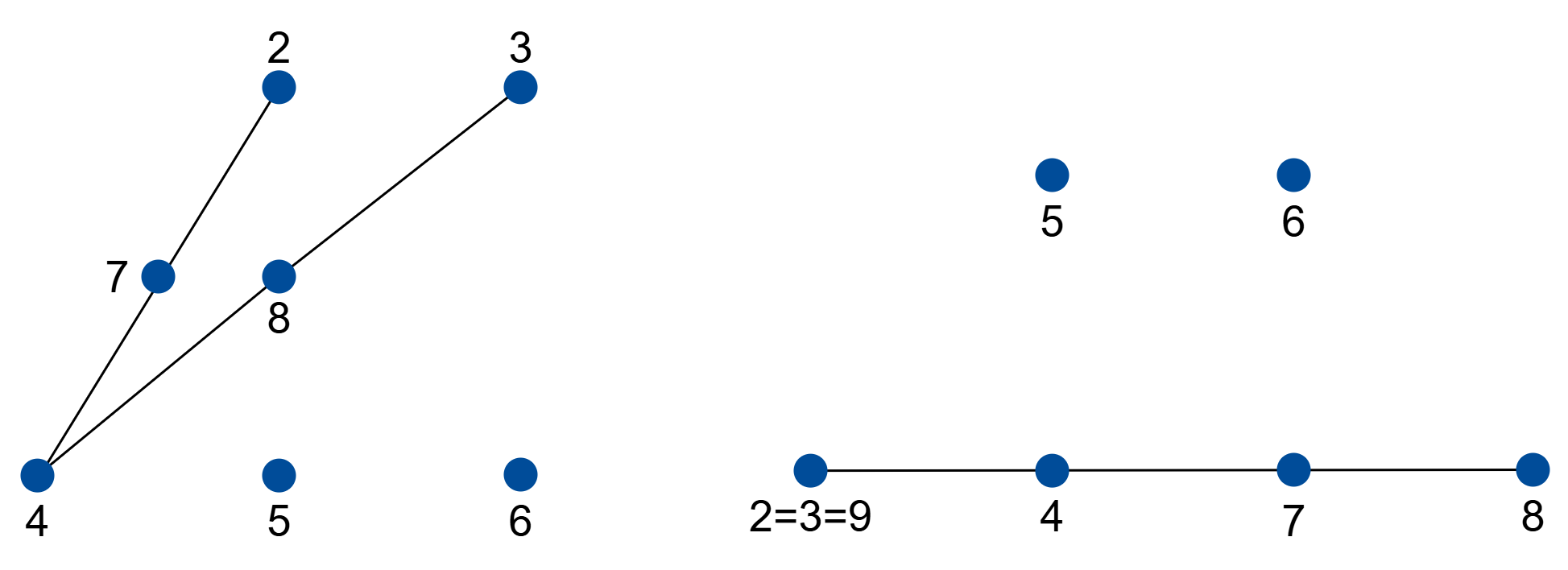
Figure 4: (Left) Matroid $\displaystyle N\backslash\{9\}$; (Right) Matroid $\displaystyle A$. Both arise in the proof of Lemma 4.12.

Lemma 4.12.

Let $\displaystyle N$ be the simple rank-three matroid depicted in Figure 5 (c). Then, we have

$$V_{\mathcal{C}(N)}=V_{N}\cup V_{N(9)}.$$ (4.4)

Proof.

Let $\displaystyle\gamma\in V_{\mathcal{C}(N)}$. We will prove that $\displaystyle\gamma$ belongs to one of the varieties on the right-hand side of (4.4). First, suppose that $\displaystyle\gamma_{9}=0$. Since $\displaystyle N\backslash\{9\}$, shown in Figure 4 (Left), is nilpotent with all points of degree at most two, Theorem 2.7 (i) implies that $\displaystyle V_{\mathcal{C}(N\backslash\{9\})}=V_{N\backslash\{9\}}$, which further implies $\displaystyle V_{\mathcal{C}(N(9))}=V_{N(9)}$. From this, we conclude that $\displaystyle\gamma\in V_{N(9)}$.

Now suppose that $\displaystyle\gamma_{9}\neq 0$. Then, by Lemma 4.11, we may assume that $\displaystyle\gamma$ has no loops.

Case 1. Suppose that $\displaystyle\gamma_{2}\neq\gamma_{9}$ or $\displaystyle\gamma_{3}\neq\gamma_{9}$. Without loss of generality, assume that $\displaystyle\gamma_{2}\neq\gamma_{9}$. By Theorem 2.7 (i), we can apply a perturbation to the vectors $\displaystyle\{\gamma_{2},\gamma_{3},\gamma_{4},\gamma_{5},\gamma_{7},\gamma_{8},\gamma_{9}\}$ to obtain a collection $\displaystyle\{\widetilde{\gamma}_{2},\widetilde{\gamma}_{3},\widetilde{\gamma}_{4},\widetilde{\gamma}_{5},\widetilde{\gamma}_{7},\widetilde{\gamma}_{8},\widetilde{\gamma}_{9}\}\in\Gamma_{N\backslash\{6\}}$. Since $\displaystyle\gamma_{2}\neq\gamma_{9}$, the line spanned by $\displaystyle\widetilde{\gamma}_{2}$ and $\displaystyle\widetilde{\gamma}_{9}$ is a perturbation of the line through $\displaystyle\gamma_{2}$ and $\displaystyle\gamma_{9}$. Since the only line in $\displaystyle N$ containing the point $\displaystyle 6$ is $\displaystyle\{2,9,6\}$, we can perturb $\displaystyle\gamma_{6}$ so that it lies on the line through $\displaystyle\widetilde{\gamma}_{2}$ and $\displaystyle\widetilde{\gamma}_{9}$. This yields a collection of vectors in $\displaystyle\Gamma_{N}$, showing that $\displaystyle\gamma\in V_{N}$.

Case 2. Suppose that $\displaystyle\gamma_{2}=\gamma_{3}=\gamma_{9}$. Since $\displaystyle\{2,7,4\},\{7,8,9\}$ and $\displaystyle\{3,4,8\}$ are dependent in $\displaystyle N$ and $\displaystyle\gamma\in V_{\mathcal{C}(N)}$, the sets of vectors $\displaystyle\{\gamma_{2},\gamma_{7},\gamma_{4}\},\{\gamma_{7},\gamma_{8},\gamma_{9}\}$ and $\displaystyle\{\gamma_{3},\gamma_{4},\gamma_{8}\}$ are dependent. Moreover, using that $\displaystyle\gamma_{2}=\gamma_{3}=\gamma_{9}$, we obtain that the sets of vectors $\displaystyle\{\gamma_{2},\gamma_{7},\gamma_{4}\},\{\gamma_{2},\gamma_{7},\gamma_{8}\},\{\gamma_{2},\gamma_{4},\gamma_{8}\}$ are dependent. Hence, $\displaystyle\{\gamma_{2},\gamma_{4},\gamma_{7},\gamma_{8}\}$ are collinear in $\displaystyle\mathbb{P}^{2}$.

Let $\displaystyle A$ be the rank-three matroid on the ground set $\displaystyle\{2,\ldots,9\}$, in which $\displaystyle 2=3=9$ and the points $\displaystyle\{2,4,7,8\}$ form a line with the points $\displaystyle 5$ and $\displaystyle 6$ lying outside of it, as in Figure 4 (Right). Given that $\displaystyle\operatorname{rk}\{\gamma_{2},\gamma_{4},\gamma_{7},\gamma_{8}\}\leq 2$, it follows that $\displaystyle\gamma\in V_{\mathcal{C}(A)}$. After the identification of the double point $\displaystyle\{2,3,9\}$ as a simple point in $\displaystyle A$, the resulting matroid is nilpotent and all of its points have degree at most two. By Theorem 2.7 (i), we conclude that $\displaystyle V_{\mathcal{C}(A)}=V_{A}$. We will end by showing that $\displaystyle V_{A}\subseteq V_{N}$, which would imply $\displaystyle\gamma\in V_{A}\subset V_{N}$, completing the proof. We will use a similar technique as in [18].

Following the constructive approach outlined in the proof of [11, Theorem 4.5], we find that any element $\displaystyle\gamma\in\Gamma_{N}$ can be written as

$$\gamma=\begin{pmatrix}1&0&0&1&1+v&1&1+v&1\\ 0&1&0&1&1&0&1+z&w+zw\\ 0&0&1&1&1&w&1&w\end{pmatrix},$$ (4.5)

where the minors corresponding to the bases are nonzero, and the columns are indexed, from left to right, by $\displaystyle\{9,4,5,6,2,3,7,8\}$. To prove that $\displaystyle V_{A}\subset V_{N}$, it suffices to show that any $\displaystyle\xi\in\Gamma_{A}$ lies in $\displaystyle V_{N}$. We will show this by seeing that we can infinitesimally perturb $\displaystyle\xi$ to obtain an element in $\displaystyle\Gamma_{N}$. Following the construction in the proof of [11, Theorem 4.5], we find that any element $\displaystyle\xi\in\Gamma_{A}$ has the form

$$\xi=\begin{pmatrix}1&0&0&1&1&1&1&1\\ 0&1&0&1&0&0&x&y\\ 0&0&1&1&0&0&0&0\end{pmatrix},$$

where, the columns correspond to $\displaystyle\{9,4,5,6,2,3,7,8\}$ and the minors corresponding with the bases are non-zero. For any $\displaystyle\epsilon$, define $\displaystyle\gamma_{\epsilon}\in\Gamma_{N}$ by substituting into the parametrization (4.5) the values

$$1+v=\frac{1}{\epsilon},\quad w=\frac{\epsilon}{x}y,\quad 1+z=\frac{x}{\epsilon}.$$

As $\displaystyle\epsilon\to 0$, we get that $\displaystyle\gamma_{\epsilon}\to\xi$, which implies $\displaystyle\xi\in V_{N}$. Since $\displaystyle\xi$ was arbitrary, it follows that $\displaystyle\Gamma_{A}\in V_{N}$, and therefore $\displaystyle V_{A}\in V_{N}$, completing the proof. ∎

We now present the irreducible decomposition of the circuit variety of the Pascal configuration.

Theorem 4.13.

The circuit variety $\displaystyle V_{\mathcal{C}(M)}$ admits the following irreducible decomposition:

$$V_{\mathcal{C}(M)}=V_{M}\cup V_{U_{2,9}}\cup_{i=7}^{9}V_{M(i)}.$$ (4.6)

Proof.

The inclusion $\displaystyle\supseteq$ is clear, since the matroids on the right-hand side contain more dependencies than $\displaystyle M$. To establish the reverse inclusion, we must show that any $\displaystyle\gamma\in V_{\mathcal{C}(M)}$ lies in the variety on the right-hand side of (4.6). First, suppose that there exists $\displaystyle i\in\{7,8,9\}$ such that $\displaystyle\gamma_{i}=0$. Without loss of generality, assume $\displaystyle i=7$. Since the matroid $\displaystyle M\backslash\{7\}$, depicted in Figure 5 (d), is nilpotent without points of degree at least three, it follows that $\displaystyle V_{\mathcal{C}(M(7))}=V_{M(7)}$. Consequently, we have $\displaystyle\gamma\in V_{M(7)}$, as desired. Hence, from this point onward, we can assume that $\displaystyle\gamma_{7},\gamma_{8},\gamma_{9}\neq 0$.

Case 1. Suppose there exists $\displaystyle p\in[6]$ such that $\displaystyle\gamma_{l_{1}}\wedge\gamma_{l_{2}}\neq 0$, where $\displaystyle\{l_{1},l_{2}\}=\mathcal{L}_{p}$. Without loss of generality, assume $\displaystyle p=1$. Since $\displaystyle M\backslash\{1\}$ is the matroid from Lemma 4.12, applying this result yields $\displaystyle{\left.\kern-1.2pt\gamma\vphantom{\small|}\right|_{\{2,\ldots,9\}}}\in V_{M\backslash\{1\}}$. Consequently, we can perturb $\displaystyle\{\gamma_{2},\ldots,\gamma_{9}\}$ to obtain a collection $\displaystyle\{\widetilde{\gamma}_{2},\ldots,\widetilde{\gamma}_{9}\}$ in $\displaystyle\Gamma_{M\backslash\{1\}}$. Extending $\displaystyle\widetilde{\gamma}$ by defining $\displaystyle\widetilde{\gamma}_{1}=\widetilde{\gamma}_{5}\widetilde{\gamma}_{7}\wedge\widetilde{\gamma}_{6}\widetilde{\gamma}_{8}$, we obtain $\displaystyle\widetilde{\gamma}\in V_{M}$, which implies $\displaystyle\gamma\in V_{M}$.

Case 2. Suppose that for all points $\displaystyle p\in[6]$, it holds that $\displaystyle\gamma_{l_{1}}\wedge\gamma_{l_{2}}=0$, where $\displaystyle\{l_{1},l_{2}\}=\mathcal{L}_{p}$.

Case 2.1. Suppose there exists $\displaystyle p\in[6]$ such that $\displaystyle\gamma_{p}=0$. Since this point lies on exactly two lines in $\displaystyle M$, we can redefine $\displaystyle\gamma_{p}$ as a nonzero vector in the intersection $\displaystyle\gamma_{l_{1}}\cap\gamma_{l_{2}}$ of the two lines it belongs to, where $\displaystyle\mathcal{L}_{p}=\{l_{1},l_{2}\}$. Thus, we may henceforth assume that $\displaystyle\gamma$ contains no loops.

Case 2.2. Suppose there exists $\displaystyle i\in[6]$ and $\displaystyle j\in[9]$ with $\displaystyle i\neq j$ such that $\displaystyle\gamma_{i}=\gamma_{j}$. Without loss of generality, assume $\displaystyle i=1$. First suppose that $\displaystyle\operatorname{rk}\{\gamma_{1},\gamma_{6},\gamma_{8}\}=2$ or $\displaystyle\operatorname{rk}\{\gamma_{1},\gamma_{5},\gamma_{7}\}=2$. By assumption, this implies that the corresponding two lines coincide. Consequently, we can perturb $\displaystyle\gamma_{1}$ to any other vector $\displaystyle\widetilde{\gamma}_{1}$ on this line, ensuring that $\displaystyle\widetilde{\gamma}_{1}\neq\gamma_{j}$, while still remaining in $\displaystyle V_{\mathcal{C}(M)}$. Now suppose that $\displaystyle\operatorname{rk}\{\gamma_{1},\gamma_{6},\gamma_{8}\}=1$ and $\displaystyle\operatorname{rk}\{\gamma_{1},\gamma_{5},\gamma_{7}\}=1$. In this case, we can perturb $\displaystyle\gamma_{1}$ to any other vector $\displaystyle\widetilde{\gamma}_{1}$, ensuring that $\displaystyle\widetilde{\gamma}_{1}\neq\gamma_{j}$, while still remaining in $\displaystyle V_{\mathcal{C}(M)}$. Thus, we may assume henceforth that there do not exist $\displaystyle i\in[6]$ and $\displaystyle j\in[9]$ with $\displaystyle i\neq j$ such that $\displaystyle\gamma_{i}=\gamma_{j}$.

Case 2.3. Suppose that Cases 2.1 and 2.2 do not apply. Observe that for every line $\displaystyle l$ of $\displaystyle M$ distinct from $\displaystyle\{7,8,9\}$, the set $\displaystyle\{\gamma_{p}:p\in l\}$ contains three different points and no loops, implying that $\displaystyle\operatorname{rk}(\gamma_{l})=2$. By our assumption in Case 2, these six lines must coincide, that is,

$$\gamma_{\{1,6,8\}}=\gamma_{\{1,5,7\}}=\gamma_{\{2,6,9\}}=\gamma_{\{2,7,4\}}=\gamma_{\{3,4,8\}}=\gamma_{\{3,5,9\}}.$$

It follows that the vectors $\displaystyle\{\gamma_{1},\ldots,\gamma_{9}\}$ all lie in a common two-dimensional subspace. Consequently, we conclude that $\displaystyle\gamma\in V_{\mathcal{C}(U_{2,9})}=V_{U_{2,9}}$.

The irreducibility of the varieties in (4.6) follows from Theorem 2.7(ii). Moreover, one can easily prove that there are no redundant components in this decomposition. This establishes that the decomposition is indeed the irredundant irreducible decomposition, thereby completing the proof. ∎

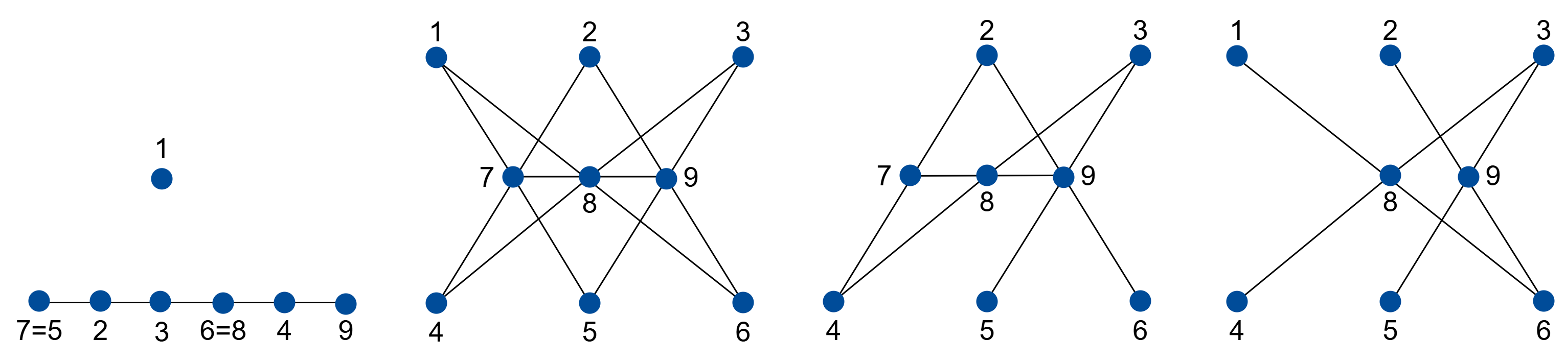
Figure 5: Form left to right: (a) $\displaystyle\pi_{M}^{1}$; (b) Pascal configuration ; (c) Pascal configuration without the point 1 ;(d) Pascal configuration without the point 7.

4.2.2 Matroid ideal of Pascal configuration

We will now provide a generating set for the matroid ideal of the Pascal configuration, up to radical.

Theorem 4.14.

Let $\displaystyle M$ be the matroid associated to the Pascal configuration. Then

$$I_{M}=\sqrt{I_{\mathcal{C}(M)}+G_{M}+I_{M}^{\textup{lift}}}.$$

Proof.

To prove the equality of the statement, we will show the following equivalent equality of varieties

$$V_{M}=V_{\mathcal{C}(M)}\cap V(G_{M})\cap V_{M}^{\textup{lift}}.$$ (4.7)

The inclusion $\displaystyle\subset$ in (4.7) follows directly from Theorem 2.12 and Proposition 2.16. To establish the reverse inclusion, let $\displaystyle\gamma\in V(G_{M})\cap V(I_{M}^{\textup{lift}})\cap V_{\mathcal{C}(M)}$. Since $\displaystyle\gamma\in V_{\mathcal{C}(M)}$, by Theorem 4.13 we have

$$\gamma\in V_{M}\cup V_{U_{2,9}}\cup_{i=7}^{9}V_{M(i)}.$$ (4.8)

Case 1. Suppose that $\displaystyle\text{rk}(\gamma)=3$.

Case 1.1. Suppose that $\displaystyle\gamma_{7},\gamma_{8},\gamma_{9}\neq 0$. Since $\displaystyle\operatorname{rk}(\gamma)=3$, we deduce that $\displaystyle\gamma\not\in V_{U_{2,9}}$. Additionally, because $\displaystyle\gamma_{7},\gamma_{8},\gamma_{9}\neq 0$, we have $\displaystyle\gamma\not\in\cup_{i=7}^{9}V_{M(i)}$. Thus, from (4.8), it follows that $\displaystyle\gamma\in V_{M}$, as desired.

Case 1.2 Suppose there exists a loop $\displaystyle\gamma_{i}$ for some $\displaystyle i\in\{7,8,9\}$. If there are at least two distinct lines $\displaystyle l\in\mathcal{L}_{i}$ with $\displaystyle\text{rk}(\gamma_{l})=2$, then, since $\displaystyle\gamma\in V(G_{M})$, Proposition 2.16 ensures that these lines intersect nontrivially. In this case, we redefine $\displaystyle\gamma_{i}$ as the intersection of these lines. After applying this procedure to all such loops, we may assume that each remaining loop has at most one line $\displaystyle l\in\mathcal{L}_{i}$ with $\displaystyle\text{rk}(l)=2$.

Now perturb $\displaystyle\gamma_{i}$ to a nonzero vector in $\displaystyle\gamma_{l}$ for some $\displaystyle l\in\mathcal{L}_{i}$ with $\displaystyle\text{rk}(l)=2$. If no such line exists, we redefine $\displaystyle\gamma_{i}$ arbitrarily. The resulting configuration remains in $\displaystyle V_{\mathcal{C}(M)}$, since any line passing through $\displaystyle\gamma_{i}$ with rank one will still have rank at most two after this perturbation. Repeating this process for all points in $\displaystyle\{7,8,9\}$, we redefine $\displaystyle\gamma$ such that $\displaystyle\gamma_{7},\gamma_{8},\gamma_{9}\neq 0$ while ensuring that the configuration remains in $\displaystyle V_{\mathcal{C}(M)}$. At this stage, we fall into Case 1.1, from which it follows that $\displaystyle\gamma\in V_{M}$, as desired.

Case 2. Suppose that $\displaystyle\text{rk}(\gamma)=2$. In this case, all vectors of $\displaystyle\gamma$ lie on a single line in the projective plane, which we denote by $\displaystyle l$.

Case 2.1. Suppose that $\displaystyle\gamma_{7},\gamma_{8},\gamma_{9}\neq 0$. Since $\displaystyle\gamma\in V(I_{M}^{\textup{lift}})$, we can use Theorem 2.12 to lift $\displaystyle\gamma$ to $\displaystyle\widetilde{\gamma}\in V_{\mathcal{C}(M)}$, such that $\displaystyle\text{rk}(\widetilde{\gamma})=3$ and $\displaystyle\widetilde{\gamma}_{7},\widetilde{\gamma}_{8},\widetilde{\gamma}_{9}\neq 0$. By Case 1.1, this ensures that $\displaystyle\widetilde{\gamma}\in V_{M}$, and consequently $\displaystyle\gamma\in V_{M}$, as desired.

Case 2.2. Suppose that at least one of $\displaystyle\gamma_{7},\gamma_{8},\gamma_{9}$ is a loop. If multiple elements in $\displaystyle\{\gamma_{7},\gamma_{8},\gamma_{9}\}$ are loops, redefine all but one of them as arbitrary points on $\displaystyle l$. Consequently, we may assume without loss of generality that the only loop in $\displaystyle\{\gamma_{7},\gamma_{8},\gamma_{9}\}$ is $\displaystyle\gamma_{7}$. Let $\displaystyle q\in\mathbb{P}^{2}$ be any point outside $\displaystyle l$. By Theorem 4.4, we obtain $\displaystyle\operatorname{dim}_{q}^{\gamma}(M\backslash\{7\})=\operatorname{dim}_{q}^{\gamma}(S_{M})=4$. Applying Proposition 4.8, we can redefine $\displaystyle\gamma_{7}$ as a point on $\displaystyle l$ such that the resulting configuration is liftable. Thus, we can perturb $\displaystyle\gamma$ to $\displaystyle\widetilde{\gamma}\in V_{M}$.

Case 3. Suppose that $\displaystyle\text{rk}(\gamma)=1$. In this case, all points either coincide at a fixed point or are loops. If at least one point is a loop, perturb the remaining points to reduce to Case 2.2. If there are no loops, then all points coincide. We will use the same technique as in [18]. By applying a projective transformation, we may assume that this common point is $\displaystyle(1,0,0)$.

Following the constructive approach outlined in the proof of [11, Theorem 4.5], we find that any element of $\displaystyle\Gamma_{M}$ can be expressed as

$$\begin{pmatrix}1&1&1&1&1+x&1+y&1+y+z&-(1+z)(x+1)+1+y+z&2x+1\\ 0&\epsilon&0&\epsilon&\epsilon&\epsilon&\epsilon+\epsilon z&0&(1+z)\epsilon\\ 0&0&\eta&\eta&0&\eta&\eta&\eta&\eta x\end{pmatrix}.$$

Letting $\displaystyle x,y,\eta,\epsilon,z\to 0$, we see that the configuration in which all points coincide can be realized as a limit of configurations in $\displaystyle\Gamma_{M}$. It follows that $\displaystyle\gamma\in V_{M}$. ∎

Although Theorem 4.14 establishes that the ideals $\displaystyle I_{\mathcal{C}(M)},G_{M}$ and $\displaystyle I_{M}^{\textup{lift}}$ generate $\displaystyle I_{M}$ up to radical, it does not present an explicit generating set. The following remark addresses this point.

Remark 4.15.

By Theorem 4.14, to find explicit generators for $\displaystyle I_{M}$, up to radical, it suffices to find explicit generators for $\displaystyle I_{\mathcal{C}(M)},G_{M}$ and $\displaystyle I_{M}^{\textup{lift}}$.

• The circuit polynomials are precisely the bracket polynomials corresponding to the circuits of $\displaystyle M$, see Remark 2.6. In this case, they are: $\displaystyle\bigl{\{}[168],[157],[247],[269],[348],[359],[789]\bigr{\}}.$

• Regarding the Grassmann–Cayley polynomials in $\displaystyle G_{M}$, an inspection of the proof of Theorem 4.14 gives that it suffices to consider the following polynomials:

  • $\displaystyle[153][142][546][326]-[154][132][536][426]$ arising from $\displaystyle(15\wedge 24)\vee(16\wedge 34)\vee(35\wedge 26)=0$.

  • $\displaystyle[526][361][734]-[326][361][754]+[326][461][753]$ corresponding to $\displaystyle 7\vee(53\wedge 26)\vee(34\wedge 61)=0$, along with the two analogous polynomials in $\displaystyle G_{M}$ obtained from the expressions

    $$8\vee(51\wedge 24)\vee(35\wedge 62)=0,\qquad\text{and}\qquad 9\vee(43\wedge 16)\vee(24\wedge 51)=0.$$

  • $\displaystyle[749][361]-[461][739]\in G_{M}$ corresponding to the expression $\displaystyle 7\vee 9\vee(34\wedge 61)=0$, together with its two analogues derived from

    $$7\vee 8\vee(35\wedge 62)=0,\qquad\text{and}\qquad 9\vee 8\vee(15\wedge 42)=0.$$

  These are precisely the seven Grassmann–Cayley polynomials identified in [24, Theorem 3.0.2]. We refer the reader to that work for the details.

• Looking into the proof of Theorem 4.14, we note that we only use the assumption $\displaystyle\gamma\in V(I_{M}^{\textup{lift}})$ to ensure the existence of a non-degenerate lifting of $\displaystyle\{\gamma_{1},\ldots,\gamma_{9}\}$ to a collection in $\displaystyle V_{\mathcal{C}(M)}$. Thus, by [17, Lemma 3.6], it suffices to consider the $\displaystyle 7\times 7$ minors of the liftability matrices $\displaystyle\mathcal{M}_{q}(M)$.

  Although the set of all such minors is not finite, since $\displaystyle q$ ranges over $\displaystyle\mathbb{C}^{3}$, the discussion in [17, §6] shows that one obtains a finite generating set by selecting vectors $\displaystyle q_{1},\ldots q_{9}\in\mathbb{C}^{3}$ and replacing the vector $\displaystyle q$ appearing in the brackets of column $\displaystyle i$ with $\displaystyle q_{i}$. This also gives us a polynomial inside $\displaystyle I_{M}$. By multilinearity of the determinant, it is enough to take each $\displaystyle q_{i}$ from the canonical basis $\displaystyle\{e_{1},e_{2},e_{3}\}$ of $\displaystyle\mathbb{C}^{3}$. The resulting polynomials are the $\displaystyle 7\times 7$ minors of the matrices

  $$\begin{pmatrix}[68q_{1}]&0&0&0&0&-[18q_{6}]&0&[16q_{8}]&0\\ [57q_{1}]&0&0&0&-[17q_{5}]&0&[15q_{7}]&0&0\\ 0&[47q_{2}]&0&-[27q_{4}]&0&0&[24q_{7}]&0&0\\ 0&[69q_{2}]&0&0&0&-[29q_{6}]&0&0&[26q_{9}]\\ 0&0&[48q_{3}]&-[38q_{4}]&0&0&0&[34q_{8}]&0\\ 0&0&[59q_{3}]&0&-[39q_{5}]&0&0&0&[35q_{9}]\\ 0&0&0&0&0&0&[89q_{7}]&-[79q_{8}]&[78q_{9}]\\ \end{pmatrix},$$

  where $\displaystyle q_{1},\ldots,q_{9}\in\{e_{1},e_{2},e_{3}\}$. The total number of such polynomials is $\displaystyle\textstyle\binom{9}{7}3^{9}=708{,}588$.

4.3 Pappus configuration

We now study the Pappus configuration, the simple rank-three matroid in Figure 6 (Left). Specifically, we find a finite generating set for its matroid ideal. In this subsection, we denote this matroid by $\displaystyle M$.

We first state the following result from [18, §5.4].

Theorem 4.16.

The circuit variety of $\displaystyle M$ admits the following irreducible decomposition

$$V_{\mathcal{C}(M)}=V_{M}\cup V_{U_{2,9}}\cup_{i=1}^{18}V_{I_{i}}\cup_{i=1}^{3}V_{J_{i}}\cup_{i=1}^{9}V_{\pi_{M}^{i}},$$ (4.9)

where the matroids in the decomposition are the following:

• $\displaystyle U_{2,9}$ denotes the uniform matroid of rank two on the ground set $\displaystyle[9]$, see Definition 2.1.

• We denote by $\displaystyle I_{i}$ for $\displaystyle i\in[18]$ the matroid obtained from $\displaystyle M$ by making one of its points a loop and adding one of the circuits $\displaystyle\{1,4,9\},\{2,5,8\}$ or $\displaystyle\{3,6,7\}$, see Figure 6 (Center).

• We denote $\displaystyle J_{1},J_{2},J_{3}$ for the matroids derived from $\displaystyle M$ by making loops all three points of one of the triples $\displaystyle\{1,4,9\},\{3,6,7\}$ or $\displaystyle\{2,5,8\}$, see Figure 6 (Right).

• The matroids $\displaystyle\pi_{M}^{i}$ are defined in Notation 4.9. See Figure 7 (Left) for an illustration.

To determine the defining equations of $\displaystyle M$, we use the following proposition, which decomposes the circuit variety of the matroids $\displaystyle M(i)$ obtained from $\displaystyle M$ by making one point a loop. Since all cases are analogous, we focus on $\displaystyle i=9$ in the proposition below.

Proposition 4.17.

The circuit variety of $\displaystyle M(9)$ from Figure 7 (Center) satisfies:

$$V_{\mathcal{C}(M(9))}=V_{M(9)}\cup V_{U_{2,9}(9)}\cup_{j=1,4}V_{M(9,j)}\cup V_{M(1,4,9)}.$$ (4.10)

Proof.

The decomposition of $\displaystyle V_{\mathcal{C}(M(9))}$ corresponds to that of $\displaystyle V_{\mathcal{C}(M\backslash\{9\})}$, so it suffices to decompose $\displaystyle V_{\mathcal{C}(M\backslash\{9\})}$. For simplicity, denote $\displaystyle N:=M\backslash\{9\}$. With this notation, it is enough to prove that:

$$V_{\mathcal{C}(N)}=V_{N}\cup V_{U_{2,8}}\cup\bigcup_{j\in\{1,4\}}V_{N(j)}\cup V_{N(1,4)}.$$ (4.11)

The inclusion $\displaystyle\supseteq$ in (4.11) is immediate since each matroid variety on the right-hand side corresponds to matroids with strictly more dependencies than $\displaystyle N$. To prove the reverse inclusion, we will show that any collection $\displaystyle\gamma\in V_{\mathcal{C}(N)}$ must lie in one of the varieties appearing on the right-hand side of (4.11).

Suppose first that either $\displaystyle\gamma_{1}=0$ or $\displaystyle\gamma_{4}=0$, and without loss of generality, assume that $\displaystyle\gamma_{1}=0$. The matroid $\displaystyle M(1,9)$ is illustrated in Figure 7 (Right). By Lemma 5.5 (iv) of [18], we have $\displaystyle V_{\mathcal{C}(N(1))}=V_{N(1)}\cup V_{N(1,4)}$, which implies $\displaystyle\gamma\in V_{N(1)}\cup V_{N(1,4)}$.

Now assume that $\displaystyle\gamma_{1},\gamma_{4}\neq 0$. Then, by Lemma 4.11, we may assume that $\displaystyle\gamma$ has no loops.

Case 1. There exists $\displaystyle p\in[8]\backslash\{1,4\}$ such that $\displaystyle\gamma_{l_{1}}\wedge\gamma_{l_{2}}\neq 0$, where $\displaystyle\{l_{1},l_{2}\}=\mathcal{L}_{p}$.

In this case, since $\displaystyle N\backslash\{p\}$ is nilpotent and all its points have degree at most two, Theorem 2.7 (i) allows us to perturb the collection $\displaystyle\{\gamma_{i}:i\in[8]\backslash\{p\}\}$ to obtain vectors $\displaystyle\{\widetilde{\gamma}_{i}:i\in[8]\backslash\{p\}\}\in\Gamma|_{N\backslash\{p\}}$. We then extend $\displaystyle\widetilde{\gamma}$ by defining $\displaystyle\widetilde{\gamma}_{p}$ as $\displaystyle\widetilde{\gamma}_{l_{1}}\wedge\widetilde{\gamma}_{l_{2}}$, where $\displaystyle\mathcal{L}_{p}=\{l_{1},l_{2}\}$, thereby obtaining a collection $\displaystyle\widetilde{\gamma}\in V_{N}$. Since $\displaystyle\widetilde{\gamma}$ is a perturbation of $\displaystyle\gamma$, it follows that $\displaystyle\gamma\in V_{N}$, as desired.

Case 2. For all $\displaystyle p\in[8]\backslash\{1,4\}$ it holds that $\displaystyle\gamma_{l_{1}}\wedge\gamma_{l_{2}}=0$, where $\displaystyle\{l_{1},l_{2}\}=\mathcal{L}_{p}$.

Case 2.1. Suppose there exist distinct $\displaystyle i,j\in[8]$ such that either $\displaystyle i,j\in[8]\setminus\{1,4\}$ or $\displaystyle i\in[8]\setminus\{1,4\}$ and $\displaystyle j\in\{1,4\}$, for which $\displaystyle\gamma_{i}=\gamma_{j}$. Assume without loss of generality that $\displaystyle i=1$ and $\displaystyle j=2$. Since $\displaystyle\gamma_{4}\gamma_{7}\wedge\gamma_{1}\gamma_{3}=0$, the pairs $\displaystyle\{\gamma_{4},\gamma_{7}\}$ and $\displaystyle\{\gamma_{1},\gamma_{3}\}$ cannot span distinct lines in $\displaystyle\mathbb{P}^{2}$. If both pairs span the same line, then $\displaystyle\gamma_{2}$ can be perturbed to any point on that line away from $\displaystyle\gamma_{1}$, yielding a collection that remains in $\displaystyle V_{\mathcal{C}(N)}$. If both pairs span a one-dimensional space, then $\displaystyle\gamma_{2}$ can be perturbed to an arbitrary point away from $\displaystyle\gamma_{1}$, producing a collection still in $\displaystyle V_{\mathcal{C}(N)}$. Repeating this argument as needed, we may assume without loss of generality that the collection in $\displaystyle V_{\mathcal{C}(N)}$ does not present this type of double points. We now analyze this case.

Case 2.2. Suppose that $\displaystyle\gamma_{i}\neq\gamma_{j}$ for all distinct $\displaystyle i,j\in[8]\setminus\{1,4\}$, as well as for all $\displaystyle i\in[8]\setminus\{1,4\}$ and $\displaystyle j\in\{1,4\}$. Under the assumption of Case 2, we have the following equalities:

$$\gamma_{\{1,2,3\}}=\gamma_{\{2,7,4\}}=\gamma_{\{3,4,8\}}=\gamma_{\{1,6,8\}}=\gamma_{\{4,5,6\}}=\gamma_{\{1,5,7\}},$$

which imply that the vectors $\displaystyle\{\gamma_{1},\ldots,\gamma_{8}\}$ are all collinear in $\displaystyle\mathbb{P}^{2}$. Hence, $\displaystyle\gamma\in V_{U_{2,8}}$, as desired.

∎

We now present the main result of this subsection, a generating set for the matroid ideal $\displaystyle I_{M}$.

Theorem 4.18.

Let $\displaystyle M$ be the matroid associated to the Pappus configuration. Then

$$I_{M}=\sqrt{I_{\mathcal{C}(M)}+G_{M}+I_{M}^{\textup{lift}}}.$$

Proof.

To prove the equality of the statement, we will show the following equivalent equality of varieties

$$V_{M}=V_{\mathcal{C}(M)}\cap V(G_{M})\cap V_{M}^{\textup{lift}}.$$ (4.12)

The inclusion $\displaystyle\subset$ in (4.12) follows directly from Theorem 2.12 and Proposition 2.16. To prove the reverse inclusion, let $\displaystyle\gamma\in V(G_{M})\cap V_{M}^{\text{lift}}\cap V_{\mathcal{C}(M)}$. To show that $\displaystyle\gamma\in V_{M}$, we consider the following cases:

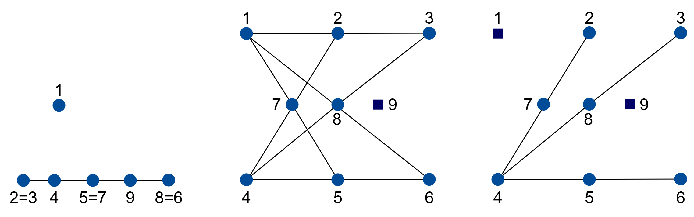
Figure 7: (Left) $\displaystyle\pi_{M}^{i}$; (Center) $\displaystyle M(9)$; (Right) $\displaystyle M(1,9)$.

Case 1. $\displaystyle\gamma$ has no loops.

In this case, Theorem 4.16 shows that $\displaystyle\gamma\in V_{U_{2,9}}$ or $\displaystyle\gamma\in V_{\pi_{M}^{i}}$ for some $\displaystyle i\in[9]$ or $\displaystyle\gamma\in V_{M}$. Since we must prove that $\displaystyle\gamma\notin V_{M}$, it remains to consider the first two possibilities.

Case 1.1. Suppose that $\displaystyle\gamma\in V_{\pi_{M}^{i}}$ for some $\displaystyle i\in[9]$. Then, all vectors of $\displaystyle\gamma$, except one, lie on a line in $\displaystyle\mathbb{P}^{2}$. Without loss of generality, assume this exceptional vector corresponds to the point $\displaystyle 1$. Since $\displaystyle M\backslash\{1\}$ is a full-rank submatroid of $\displaystyle M$, Theorem 2.12 allows us to infinitesimally lift the vectors $\displaystyle\{\gamma_{2},\ldots,\gamma_{9}\}$ from $\displaystyle\gamma_{1}$, to obtain vectors $\displaystyle\{\widetilde{\gamma}_{2},\ldots,\widetilde{\gamma}_{9}\}\in V_{\mathcal{C}(M\backslash\{1\})}$ with $\displaystyle\operatorname{rank}\{\gamma_{2},\ldots,\gamma_{9}\}=3$. Letting $\displaystyle\widetilde{\gamma}$ denote the resulting modified collection, we have $\displaystyle\widetilde{\gamma}\in V_{\mathcal{C}(M)}$. Since $\displaystyle\widetilde{\gamma}$ has no loops and every subset of eight vectors has rank three, it follows from Theorem 4.16 that $\displaystyle\widetilde{\gamma}\in V_{M}$.

Case 1.2. Suppose that $\displaystyle\gamma\in V_{U_{2,9}}$. Since $\displaystyle\gamma\in V_{M}^{\text{lift}}$, we can infinitesimally lift the configuration from an arbitrary point to obtain a non-degenerate configuration $\displaystyle\widetilde{\gamma}\in V_{\mathcal{C}(M)}$. If $\displaystyle\widetilde{\gamma}\in V_{M}$, the claim follows. Otherwise, $\displaystyle\widetilde{\gamma}\in V_{\pi_{M}^{i}}$ for some $\displaystyle i\in[9]$. Without loss of generality, assume $\displaystyle i=1$. Since arbitrarily small perturbations do not create new dependencies, this forces the original configuration to satisfy $\displaystyle\gamma_{2}=\gamma_{3},\gamma_{5}=\gamma_{7},\gamma_{6}=\gamma_{8}$. By perturbing $\displaystyle\gamma_{1}$ slightly so that it no longer lies on the line spanned by $\displaystyle\{\gamma_{2},\cdots,\gamma_{9}\}$, we reduce to the setting of Case 1.1, which implies that $\displaystyle\gamma\in V_{M}$.

Case 2. $\displaystyle\gamma$ has exactly one loop.

Without loss of generality, assume that the loop corresponds to $\displaystyle 9$. By Lemma 5.5 (iii) of [18], we have $\displaystyle V_{M(9)}\subseteq V_{M}$, so it suffices to prove that $\displaystyle\gamma\in V_{M(9)}$. The matroid $\displaystyle M(9)$ is shown in Figure 7 (Center). According to Equation (4.10), either $\displaystyle\gamma\in V_{M(9)}$ or $\displaystyle\gamma\in V_{U_{2,9}(9)}$. If the former holds, then $\displaystyle\gamma\in V_{M}$, as desired. Otherwise, assume $\displaystyle\gamma\in V_{U_{2,9}(9)}$. Since $\displaystyle\gamma\in V_{M}^{\text{lift}}$, we can infinitesimally lift the vectors $\displaystyle\{\gamma_{1},\ldots,\gamma_{8}\}$ from an arbitrary vector $\displaystyle q$ outside their span, yielding a non-degenerate collection $\displaystyle\{\widetilde{\gamma}_{1},\ldots,\widetilde{\gamma}_{8}\}$ of rank three in $\displaystyle V_{\mathcal{C}(M\backslash\{9\})}$. Denote by $\displaystyle\widetilde{\gamma}$ the perturbed collection of vectors, where $\displaystyle\widetilde{\gamma}_{9}=0$. Then $\displaystyle\widetilde{\gamma}$ does not have any loops apart from $\displaystyle\widetilde{\gamma}_{9}$ and is non-degenerate, so it must be in $\displaystyle V_{M(9)}$. Since $\displaystyle V_{M(9)}\subseteq V_{M}$ and $\displaystyle\widetilde{\gamma}$ is a perturbation of $\displaystyle\gamma$, we conclude that $\displaystyle\gamma\in V_{M}$.

Case 3. $\displaystyle\gamma$ has exactly two loops.

Case 3.1. Suppose the two loops correspond to elements in $\displaystyle[9]$ that do not lie on a common line in $\displaystyle M$. Without loss of generality, assume these loops correspond to $\displaystyle 1$ and $\displaystyle 9$. The matroid $\displaystyle M(1,9)$ is illustrated in Figure 7 (Right).

Case 3.1.1. Assume that the vectors $\displaystyle\gamma_{2},\ldots,\gamma_{8}$ are collinear. By applying a small perturbation within the line they span, we may further assume that they are pairwise distinct. By Theorem 4.4, $\displaystyle\operatorname{dim}_{q}^{\gamma}(M\backslash\{1,9\})=1+3=4$, where $\displaystyle q\in\mathbb{C}^{3}$ is any vector in general position with respect to $\displaystyle\gamma$. Moreover, $\displaystyle M\backslash\{1,9\}$ is nilpotent, the point $\displaystyle 1$ has degree three in $\displaystyle M$, and all the $\displaystyle\gamma_{i}$ are pairwise distinct and nonzero for $\displaystyle i\in\{2,\ldots,8\}$. We may then apply Proposition 4.8 to redefine $\displaystyle\gamma_{1}$ along the line spanned by $\displaystyle\gamma_{2},\ldots,\gamma_{8}$, so that $\displaystyle\gamma|_{[8]}\in V_{M\backslash\{9\}}^{\mathrm{lift}}$. This reduces to Case 2, from which we conclude that $\displaystyle\gamma\in V_{M}$.

Case 3.1.2. Suppose now that $\displaystyle\operatorname{rank}\{\gamma_{2},\ldots,\gamma_{8}\}=3$. One can redefine $\displaystyle\gamma_{1}$ from zero to a point lying on all the lines $\displaystyle\gamma_{l}\subset\mathbb{P}^{2}$ for which $\displaystyle l$ is a line of $\displaystyle M$ containing $\displaystyle 1$. Since $\displaystyle\gamma\in V(G_{M})$, Proposition 2.16 ensures that these lines intersect nontrivially in $\displaystyle\mathbb{P}^{2}$. Then the collection of vectors remains within $\displaystyle V_{\mathcal{C}(M(9))}$. Let $\displaystyle\widetilde{\gamma}$ denote this modified collection. Given that $\displaystyle\widetilde{\gamma}\in V_{\mathcal{C}(M(9))}$, has rank three, and contains only one loop, it follows from Equation (4.10) that $\displaystyle\widetilde{\gamma}\in V_{M(9)}$. Since $\displaystyle V_{M(9)}\subset V_{M}$, we deduce that $\displaystyle\widetilde{\gamma}\in V_{M}$. Because $\displaystyle\widetilde{\gamma}$ is a perturbation of $\displaystyle\gamma$, it follows that $\displaystyle\gamma\in V_{M}$.

Case 3.2. Suppose the two loops correspond to elements of $\displaystyle[9]$ that lie on a common line in $\displaystyle M$. In this case, by Lemma 5.5 (ii) of [18], the circuit variety of this matroid is contained within that of $\displaystyle V_{M}$.

Case 4. There are three loops.

Case 4.1. Suppose that two of the three loops correspond to elements of $\displaystyle[9]$ that lie on a common line in $\displaystyle M$. In this case, by Lemma 5.5 (ii) of [18], the circuit variety of $\displaystyle M$ is a subset of $\displaystyle V_{M}$.

Case 4.2. Suppose that no two of the three loops correspond to elements of $\displaystyle[9]$ that lie on a common line in $\displaystyle M$. In this case, we may assume, without loss of generality, that the loops correspond to the elements $\displaystyle 1$, $\displaystyle 4$, and $\displaystyle 9$. Since $\displaystyle\gamma\in V(G_{M})$, we can redefine $\displaystyle\gamma_{4}$ as a nonzero vector while keeping the collection of vectors within $\displaystyle V_{\mathcal{C}(M)}$. This reduces us to Case 3, where the argument relies only on the concurrency of the lines $\displaystyle\gamma_{\{1,2,3\}}$, $\displaystyle\gamma_{\{1,6,8\}}$, and $\displaystyle\gamma_{\{1,5,7\}}$, a property that holds after the perturbation.

Case 5. There are at least four loops.

In this case, at least two of these four loops correspond to elements in $\displaystyle[9]$ that belong to a common line in $\displaystyle M$. It then follows from Lemma 5.5(ii) of [18] that the circuit variety of $\displaystyle M$ is a subset of $\displaystyle V_{M}$.

We have established that $\displaystyle\gamma\in V_{M}$ in each of the possible cases, thereby completing the proof. ∎

Although Theorem 4.18 establishes that the ideals $\displaystyle I_{\mathcal{C}(M)}$, $\displaystyle G_{M}$, and $\displaystyle I_{M}^{\textup{lift}}$ generate $\displaystyle I_{M}$ up to radical, it does not provide an explicit generating set. The following remark addresses this point.

Remark 4.19.

By Theorem 4.14, to find explicit generators for $\displaystyle I_{M}$, up to radical, it suffices to find explicit generators for $\displaystyle I_{\mathcal{C}(M)},G_{M}$ and $\displaystyle I_{M}^{\textup{lift}}$.

• The circuit polynomials are: $\displaystyle\bigl{\{}[123],[168],[157],[247],[269],[789],[456],[348],[359]\bigr{\}}.$

• Concerning the Grassmann–Cayley polynomials, by the proof of Theorem 4.18, it suffices to consider the nine polynomials arising from the nine triples of concurrent lines in $\displaystyle M$ given by:

  $$\bigl{\{} [35][68]-[37][68],[34][69]-[37][69],[24][59]-[28][59],$$

  $$[41][89]-[45][89],[91][34]-[96][34],[63][78]-[65][78],$$

  $$[73][56]-[78][56],[61][39]-[67][39],[91][45]-[98][45]\bigr{\}}.$$

• From the proof of Theorem 4.18, we observe that the only instances where the assumption $\displaystyle\gamma\in V(I_{M}^{\textup{lift}})$ is used are: (1) to guarantee the existence of a non-degenerate lifting of the vectors $\displaystyle\{\gamma_{1},\ldots,\gamma_{9}\}$ to a collection in $\displaystyle V_{\mathcal{C}(M)}$, and (2) to ensure that for each $\displaystyle i\in[9]$, the eight vectors $\displaystyle\{\gamma_{1},\ldots,\gamma_{i-1},\hat{\gamma}_{i},\gamma_{i+1},\ldots,\gamma_{9}\}$ have a non-degenerate lifting to a collection in $\displaystyle V_{\mathcal{C}(M\backslash\{i\})}$. Thus, by [17, Lemma 3.6], it suffices to consider the $\displaystyle 7\times 7$ minors of the liftability matrices $\displaystyle\mathcal{M}_{q}(M)$, together with the $\displaystyle 6\times 6$ minors of the liftability matrices $\displaystyle\mathcal{M}_{q}(M\backslash\{i\})$ for $\displaystyle i\in[9]$.

  Although the set of all such minors is not finite, since $\displaystyle q$ ranges over $\displaystyle\mathbb{C}^{3}$, we may adopt the same strategy used in Remark 4.15 to obtain a finite generating set. Namely, we select vectors $\displaystyle q_{1},\ldots,q_{9}\in\{e_{1},e_{2},e_{3}\}$ and replace the vector $\displaystyle q$ appearing in the bracket of column $\displaystyle i$ with $\displaystyle q_{i}$. The resulting polynomials are the $\displaystyle 7\times 7$ minors of the matrices

  $$\begin{pmatrix}[23q_{1}]&[-13q_{2}]&[12q_{3}]&0&0&0&0&0&0\\ [68q_{1}]&0&0&0&0&-[18q_{6}]&0&[16q_{8}]&0\\ [57q_{1}]&0&0&0&-[17q_{5}]&0&[15q_{7}]&0&0\\ 0&[47q_{2}]&0&-[27q_{4}]&0&0&[24q_{7}]&0&0\\ 0&[69q_{2}]&0&0&0&-[29q_{6}]&0&0&[26q_{9}]\\ 0&0&[48q_{3}]&-[38q_{4}]&0&0&0&[34q_{8}]&0\\ 0&0&[59q_{3}]&0&-[39q_{5}]&0&0&0&[35q_{9}]\\ 0&0&0&0&0&0&[89q_{7}]&-[79q_{8}]&[78q_{9}]\\ 0&0&0&[56q_{4}]&-[46q_{5}]&[45q_{6}]&0&0&0\end{pmatrix},$$

  where $\displaystyle q_{1},\ldots,q_{9}\in\{e_{1},e_{2},e_{3}\}$, and the $\displaystyle 6\times 6$ minors of the matrices

  $$\begin{pmatrix}[23q_{1}]&[-13q_{2}]&[12q_{3}]&0&0&0&0&0\\ [68q_{1}]&0&0&0&0&-[18q_{6}]&0&[16q_{8}]\\ [57q_{1}]&0&0&0&-[17q_{5}]&0&[15q_{7}]&0\\ 0&[47q_{2}]&0&-[27q_{4}]&0&0&[24q_{7}]&0\\ 0&0&[48q_{3}]&-[38q_{4}]&0&0&0&[34q_{8}]\\ 0&0&0&[56q_{4}]&-[46q_{5}]&[45q_{6}]&0&0\end{pmatrix},$$

  where $\displaystyle q_{1},\ldots,q_{8}\in\{e_{1},e_{2},e_{3}\}$, along with the $\displaystyle 6\times 6$ minors of the matrices analogous to this, corresponding to omitting each index $\displaystyle i=1,\ldots,8$. The total number of such polynomials is:

  $$\textstyle\binom{9}{7}3^{9}+\binom{8}{6}3^{10}=2{,}361{,}960.$$

Acknowledgement. This work is based on the Master’s thesis of the third author. F.M and E.L were partially supported by the FWO grants G0F5921N (Odysseus) and G023721N, and the grant iBOF/23/064 from KU Leuven. E.L. was supported by PhD fellowship 1126125N.

Authors’ addresses

Emiliano Liwski, KU Leuven emiliano.liwski@kuleuven.be
Fatemeh Mohammadi, KU Leuven fatemeh.mohammadi@kuleuven.be
Lisa Vandebrouck, KU Leuven lisa.vandebrouck@student.kuleuven.be

References

- [1] W. Bruns and A. Conca. Gröbner bases and determinantal ideals. In Commutative Algebra, Singularities and Computer Algebra, pages 9–66. Springer Netherlands, 2003.
- [2] P. Caines, F. Mohammadi, E. Sáenz-de Cabezón, and H. Wynn. Lattice conditional independence models and Hibi ideals. Transactions of the London Mathematical Society, 9(1):1–19, 2022.
- [3] O. Clarke, K. Grace, F. Mohammadi, and H. Motwani. Matroid stratifications of hypergraph varieties, their realization spaces, and discrete conditional independence models. International Mathematics Research Notices, page rnac268, 2022.
- [4] O. Clarke, G. Masiero, and F. Mohammadi. Liftable point-line configurations: Defining equations and irreducibility of associated matroid and circuit varieties. Mathematics, 12(19):3041, 2024.
- [5] O. Clarke, F. Mohammadi, and H. Motwani. Conditional probabilities via line arrangements and point configurations. Linear and Multilinear Algebra, 70(20):5268–5300, 2022.
- [6] M. Drton, B. Sturmfels, and S. Sullivant. Lectures on Algebraic Statistics, volume 39. Birkhäuser, Basel, first edition, 2009.
- [7] V. Ene, J. Herzog, T. Hibi, and F. Mohammadi. Determinantal facet ideals. Michigan Mathematical Journal, 62(1):39–57, 2013.
- [8] L. M. Fehér, A. Némethi, and R. Rimányi. Equivariant classes of matrix matroid varieties. Commentarii Mathematici Helvetici, 87(4):861–889, 2012.
- [9] I. Gelfand, M. Goresky, R. MacPherson, and V. Serganova. Combinatorial geometries, convex polyhedra, and schubert cells. Advances in Mathematics, 63(3):301–316, 1987.
- [10] J. E. Graver, B. Servatius, and H. Servatius. Combinatorial rigidity. Number 2 in Mathematical Sciences Series. American Mathematical Soc., 1993.
- [11] B. Guerville-Ballé and J. Viu-Sos. Connectedness and combinatorial interplay in the moduli space of line arrangements, 2023.
- [12] R. Hartshorne. Algebraic geometry, volume 52. Springer Science & Business Media, 2013.
- [13] J. Herzog, T. Hibi, F. Hreinsdóttir, T. Kahle, and J. Rauh. Binomial edge ideals and conditional independence statements. Advances in Applied Mathematics, 3(45):317–333, 2010.
- [14] S. Hoşten and S. Sullivant. Ideals of adjacent minors. Journal of Algebra, 277(2):615–642, 2004.
- [15] B. Jackson and S.-i. Tanigawa. Maximal matroids in weak order posets. Journal of Combinatorial Theory, Series B, 165:20–46, 2024.
- [16] A. Knutson, T. Lam, and D. E. Speyer. Positroid varieties: juggling and geometry. Compositio Mathematica, 149(10):1710–1752, 2013.
- [17] E. Liwski and F. Mohammadi. Paving matroids: defining equations and associated varieties. arXiv preprint arXiv:2403.13718, 2024.
- [18] E. Liwski and F. Mohammadi. Minimal matroids in dependency posets: algorithms and applications to computing irreducible decompositions of circuit varieties. arXiv preprint arXiv:2502.00799, 2025.
- [19] E. Liwski, F. Mohammadi, and R. Prébet. Efficient algorithms for minimal matroid extensions and irreducible decompositions of circuit varieties. arXiv preprint arXiv:2504.16632, 2025.
- [20] J. Oxley. Matroid Theory. Second edition, Oxford University Press, 2011.
- [21] G. Pfister and A. Steenpass. On the primary decomposition of some determinantal hyperedge ideal. Journal of Symbolic Computation, 103:14–21, 2019.
- [22] M. J. Piff and D. J. Welsh. On the vector representation of matroids. Journal of the London Mathematical Society, 2(2):284–288, 1970.
- [23] S. Poljak and D. Turzík. Amalgamation over uniform matroids. Czechoslovak Mathematical Journal, 34(2):239–246, 1984.
- [24] J. Sidman, W. Traves, and A. Wheeler. Geometric equations for matroid varieties. Journal of Combinatorial Theory, Series A, 178:105360, 2021.
- [25] M. Sitharam and A. Vince. The maximum matroid of a graph. arXiv preprint arXiv:1910.05390.
- [26] M. Studený. Probabilistic conditional independence structures. Springer, London, 2005.
- [27] B. Sturmfels. On the matroid stratification of Grassmann varieties, specialization of coordinates, and a problem of N. White. Advances in Mathematics, 75(2):202–211, 1989.
- [28] B. Sturmfels. Algorithms in invariant theory. Springer-Verlag, Berlin, Heidelberg, 1993.
- [29] R. Vakil. The Rising Sea, Foundations of Algebraic Geometry. Available at http://math.stanford.edu/~vakil/216blog/FOAGnov1817public, 2017.
- [30] W. Whiteley. Some matroids from discrete applied geometry. Contemporary Mathematics, 197:171–312, 1996.
- [31] H. Whitney. On the abstract properties of linear dependence. Amer. J. Math., 57(3):509, jul 1935.