Anomalous diffusion and directed coalescence of condensates in driven media

Abstract

The formation of domains via phase transitions is ubiquitous across physical systems from metallic alloys to biomolecular condensates in cells. We show that when the boundaries between such domains are forced to move, for example by external electrical fields or concentration gradients, this motion internally generates dipole force fields. This translation-induced polarization leads to emergent dipole-dipole interactions that drive directed coalescence of domains, even in the absence of Brownian motion. We then ask how the stochastic motion of individual condensates is driven by active and passive stresses in viscoelastic media such as the cell cytoplasm. Our analysis reveals that active stirring can suppress or enhance the size dependence of diffusion. Together, these findings shed new light on the dynamics of condensates in viscoelastic media and conserved order parameters in general.

Phase separation contributes to intracellular organization by sorting molecules according to their relative miscibility [1, 2, 3, 4, 5, 6, 7]. The resulting biomolecular condensates have been implicated in vital processes such as gene transcription [8, 9, 10, 11, 12], splicing [13], and ribosomal subunit assembly [14, 15]. The functions of many intracellular condensates involve interactions with chromatin [16, 17] or the cytoskeleton [18, 19, 20]. This coupling to viscoelastic materials leads to passive stresses that affect the dynamics of condensates by mechanically driving ripening or arresting coarsening [21, 22, 23, 24, 25, 26]. How do active stresses generated by the cytoskeleton [27] and the correlated motion of chromatin [28, 29, 30] affect condensates? Active forces are known to accelerate diffusion [31] and are expected to facilitate the coalescence of biomolecular condensates [32]. However, stirring can also suppress phase separation [33, 34] as observed in active nematic fluids [35, 36]. Despite these recent advances, the Brownian motion of condensates in viscoelastic media is much less understood than that of rigid inclusions.

To better understand how active fluctuations in viscoelastic media drive the motion of condensates, we developed an exact analytical framework. Surprisingly, the theory universally predicts that motion induces dipole-dipole interactions between pairs of condensates. These emergent dipole-dipole interactions suggest that pairs of condensates moving according to an external concentration gradient undergo directed coalescence. This phenomenon, which we refer to as translation-induced polarization, has not been considered in prior work on phase separation in external concentration gradients [37, 38]. Translation-induced polarization is a consequence of the conservation of condensate mass under sufficiently high tension to preserve condensate shape, and is therefore not tied to any model details or nonequilibrium mechanisms. Beyond biomolecular condensates, these findings provide a new perspective on classical phase-separation kinetics [39] such as in the conserved Ising model.

Our framework is an ideal starting point for studying the dynamics of condensates in actively fluctuating viscoelastic media. We derive how the mean squared displacement of condensates will grow over time, taking into account the memory of the medium. As a specific example, we discuss how active stress fluctuations in a viscoelastic Maxwell fluid can modify the Brownian motion of the condensates. Active stresses can break the Stokes-Einstein relation by suppressing or amplifying the size dependence of condensate motion, thereby enabling greater control over condensate dynamics.

I Moving droplets generate dipole force fields

We consider condensates of biomolecules with negligible turnover on relevant timescales. This mass conservation imposes a continuity equation for the concentration $c(\bm{x},t)$ of biomolecules,

$$\partial_{t}c=\bm{\nabla}\cdot\left[M\bm{\nabla}\mu+M\bm{\nabla}\Psi-\bm{j}\right]\,,$$ (1)

with mobility $M$. In their most general form, the externally driven currents of biomolecules can be decomposed into a potential flux $-M\bm{\nabla}\Psi$, and a nonpotential flux $\bm{j}$. This general formalism can also be applied beyond the dynamics of condensates to conserved Ising models, or active matter, to name a few examples. The chemical potential, $\mu$, usually encodes a trade-off between entropy and enthalpy which depends on molecular details. Following Ref. [40], here we interpret Eq. (1) as a control problem and, therefore, the chemical potential as an unknown. Thus, all of the results in the following are independent of microscopic details.

For sufficiently high surface tension, the condensate shape is spherical with radius $R$. Assuming stable condensates, their domains $\mathcal{D}$ will change mainly due to translation and rotation, and will therefore be approximately conserved. The role of the chemical potential is to maintain phase separation with a high concentration $c(\bm{x},t)=c_{-}+\Delta c$ inside, $\bm{x}\in\mathcal{D}$, and a low concentration $c(\bm{x},t)=c_{-}$ outside the condensate. In that sense, the chemical potential can be interpreted as a Lagrangian multiplier that enforces the conservation of the shape of the condensate boundary during translation, similar to how the pressure field guarantees incompressibility in fluids. As a consequence of this conservation law, and based on the analogy to fluid mechanics, we expect that perturbations in the condensate interface propagate non-locally and induce long-range forces.

To better understand these forces, we discuss how the chemical potential $\mu$ responds to perturbations of the concentration $c$. The chemical potential satisfies a Laplace equation (1), where mass exchange enters as a source or sink. For example, a local production or degradation of biomolecules with a net rate $k(\bm{x},t)\coloneqq\partial_{t}c(\bm{x},t)$ is analogous to an electric monopole inducing an electrostatic potential [41, 42]. For a moving phase boundary, the source term $-\bm{\nabla}\cdot[\bm{v}(t)c(\bm{x},t)]=\partial_{t}c(\bm{x},t)$ is analogous to a local electric dipole—mass is removed from one point and added to a nearby point. Hence, we expect that translation will induce dipole force fields, whereas shape changes will lead to higher-order multipole fields.

In agreement with this reasoning, moving the condensate with velocity $\bm{v}(t)=\partial_{t}\bm{r}(t)$ induces an effective long-range force (Fig. 1A, Appendix A)

$$-\bm{\nabla}\mu(\bm{x},t)=\bm{\nabla}\Psi(\bm{x},t)-\frac{\Delta c}{M}\,\mathcal{B}(\bm{x}-\bm{r})\cdot\bm{v}(t)+\mathcal{O}[\bm{j}]\,,$$ (2)

where $\mathcal{B}(\bm{z})=R^{d}[\hat{\bm{z}}\otimes\hat{\bm{z}}-\bm{I}/d]/|\bm{z}|^{d}$ for large distances $|\bm{z}|\gg R$ is the Green’s tensor for a dipole field and $\mathcal{O}[\bm{j}]$ is a functional of order $\bm{j}$. Thus, we conclude that the motion of condensates, regardless of the underlying driving force, generally induces dipole force fields. We term this phenomenon translation-induced polarization as opposed to motion that arises from pre-existing polarity. Importantly, we universally predict translation-induced polarization whenever external fields are used to control domain walls.

II Motion of condensates due to potential and nonpotential forces

So far, we have focused on the emergent forces that the motion of a condensate implies. To understand how pairs of condensates interact, we now turn the tables in our framework and analyze how external forces drive the motion of a condensate. Independently of microscopic details, the velocity of the condensate is given by [40, 43]

$$\bm{v}(t)=\partial_{t}\bm{r}(t)=-\frac{d}{\Delta c}\int_{\mathcal{D}(t)}\!\frac{d^{d}\bm{x}}{V_{\mathcal{D}}}\,M\bm{\nabla}\Psi(\bm{x},t)\\ -\frac{d}{\Delta c}\int\!\frac{d^{d}\bm{x}}{V_{\mathcal{D}}}\,\mathcal{B}(\bm{x})\cdot\,\bm{j}(\bm{x},t)\,.$$ (3)

where $\mathcal{D}(t)$ indicates the time-dependent domain of a condensate centered around $\bm{r}(t)$ and $V_{\mathcal{D}}$ is its volume. This force-response relation directly follows from the chemical potential gradient, Eq. (2), together with the thermodynamic consistency criterion [40]

$$\int_{\mathcal{D}(t)}d^{d}\bm{x}\,\bm{\nabla}\mu(\bm{x})=0\,,$$ (4)

which can also be interpreted as conservation of momentum for the condensate (Appendix A). Thus, we have quantified the motion of condensates in response to locally applying potential and nonpotential forces, as well as the long-range couplings that this motion induces.

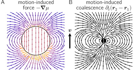
Figure 1: Emergent phenomena induced by translation with typical velocity $\bm{v}$ (black arrow) of biomolecular condensates and domain-forming systems. A) Translation leads to the emergence of long-ranged forces due to mass conservation. B) Translation leads to directed coalescence, where smaller condensates circle around and flow towards the leading edge of larger condensates.

III Pairs of moving droplets exhibit dipole-dipole interactions

Our results so far illuminate that the flow field around self-propelling condensates with nonuniform mobility, which was reported in Ref. [40], is a manifestation of the dipole force field. On the basis of these results, we predict that pairs of moving condensates show dipole-dipole interactions according to their direction of motion. These interactions emerge due to the conservation of the total mass of the phase-separating biomolecules, while the dipole and quadrupole interactions seen in active matter are mediated by the surrounding medium [44, 45, 46, 47]. What is the consequence of these emergent pairwise interactions between droplets?

For self-propelling magnetic dipoles in external flow, long-range interactions can lead to clustering [48]. We expect a similar effect for droplets in external flow, which show emergent dipolar interactions. The theory predicts that inducing condensate motion with velocity $\bm{v}$ will cause condensates of different sizes $R_{1}$ and $R_{2}$ to move relative to each other according to (Fig. 1B)

$$\partial_{t}(\bm{r}_{2}-\bm{r}_{1})\approx\left(R_{2}^{3}-R_{1}^{3}\right)\bm{\nabla}\otimes\bm{\nabla}\,\frac{1}{|\bm{r}_{2}-\bm{r}_{1}|}\cdot\bm{v}\,,$$ (5)

where $\bm{r}_{1}$ and $\bm{r}_{2}$ are the centers of mass. The smaller condensate will be drawn towards the leading side of the larger condensate, so that even passive condensates undergo directed coalescence under external potential gradients. This prediction will be tested in future experiments on condensates in external chemical gradients [49], and is consistent with the observation that diffusiophoresis of biomolecules promotes phase separation [50].

Condensate motion can also emerge as a consequence of chemical reactions without applying an external concentration gradient. Such chemical reactions can lead to effective (screened) monopole interactions [51, 41, 15], whereas the motion of condensates leads to dipole interactions. By combining these two mechanisms, we hypothesize that chemically active, self-propelling condensates [52, 53] can form stable flocks. These ideas can find potential application to mass-conserved reaction-diffusion systems if one can map them to a generalized Cahn-Hilliard model [54]. This has potentially far-reaching consequences for understanding the formation of dynamical patterns in reaction-diffusion systems.

IV Brownian motion of condensates

IV.1 Condensates in random fluid flows

Our next goal is to understand how active and passive fluctuations in the viscoelastic solvent affect condensate motion. If one zooms out to macroscopic length scales, biomolecular condensates become point-like objects defined by their positions $\bm{r}(t)$ and velocities $\bm{v}(t)=\partial_{t}\bm{r}(t)$. The motion of these point-like objects is driven by potential and nonpotential currents. In the present manuscript, we consider a fluctuating potential $\Psi$ that drives random thermal currents $\bm{j}_{th}\coloneqq-M\bm{\nabla}\Psi$ with zero mean and covariance $\langle\bm{j}_{th}(\bm{x},t)\otimes\bm{j}_{th}(\bm{x}^{\prime},t^{\prime})\rangle=2Mk_{B}T\bm{I}\delta(\bm{x}-\bm{x}^{\prime})\,\delta(t-t^{\prime})$, which is sometimes referred to as Model B [55]. Advection due to fluid flow, with flow velocity $\bm{v}_{f}$, cannot be cast as a gradient and enters through the nonpotential flux $\bm{j}\coloneqq c\,\bm{v}_{f}$. Taken together, the resulting velocity of the condensate is given by

$$\bm{v}=\frac{d}{\Delta c}\int_{\mathcal{D}(t)}\!\!\frac{d^{d}\bm{x}}{V_{\mathcal{D}}}\,\bm{j}_{th}(\bm{x},t)+\int_{\mathcal{D}(t)}\!\!\frac{d^{d}\bm{x}}{V_{\mathcal{D}}}\,\bm{v}_{f}(\bm{x},t)\,.$$ (6)

Our main focus, namely the second term in Eq. (6), intuitively states that the condensate is advected by the average flow. In the present manuscript, we neglect the feedback of condensate motion on the fluid, which is of the order $\mathcal{O}(\Delta c^{2})$ and decays as $1/M$ for large mobilities (Appendix C). Future work will investigate the resulting Casimir-like forces between condensates, and their interplay with the long-range force induced by condensate motion [Eq. (2)]. This is particularly interesting because the long-range force [Eq. (2)] only weakly affects fluid flow far away from boundaries (Appendix C), and is therefore challenging to measure.

For simplicity, we will assume that the fluid flow and the random thermal currents are independent random variables. We characterize the random Brownian motion of the condensate via the velocity autocorrelation function

$$\frac{1}{2}\partial_{t}^{2}\operatorname{MSD}(t-t^{\prime})=\langle\bm{v}(t)\cdot\bm{v}(t^{\prime})\rangle=D_{c}\,\delta(t-t^{\prime})\\ +\iint_{\mathcal{D}}\frac{d^{d}\bm{z}}{V_{\mathcal{D}}}\frac{d^{d}\bm{z}^{\prime}}{V_{\mathcal{D}}}\,\left\langle\bm{v}_{f}(\bm{r}+\bm{z},t)\cdot\bm{v}_{f}(\bm{r}^{\prime}+\bm{z}^{\prime},t^{\prime})\right\rangle\,,$$ (7)

where $\operatorname{MSD}(t-t^{\prime})\coloneqq\langle|\bm{r}(t)-\bm{r}(t^{\prime})|^{2}\rangle$ is the mean squared displacement and $D_{c}\coloneqq 2d^{3}Mk_{B}T/(\Delta c^{2}V_{\mathcal{D}})$ is an effective macroscopic diffusion coefficient. Here and in the following, we frequently use the shorthand notation $\bm{r}\equiv\bm{r}(t)$ and $\bm{r}^{\prime}\equiv\bm{r}(t^{\prime})$ for the displacement of the condensate. Note that terms lacking temporal correlations have been simplified using $\bm{r}(t)\sim\bm{r}(t^{\prime})$ because they are nonzero only for $t=t^{\prime}$. In contrast, the second line of Eq. (7) requires a more careful analysis because temporal correlations can effectively quench the flow landscape navigated by the condensates.

IV.2 Random flows at random locations

The difficulty in analyzing Eq. (7) is that not only the fluid flow but also the droplet center $\bm{r}(t)$ around which the fluid flow is evaluated are time-dependent random variables. To better understand the consequences of this geometric coupling, we consider a series expansion of the fluid flow velocity field around the midpoint $\bar{\bm{r}}\coloneqq(\bm{r}+\bm{r}^{\prime})/2$ of the condensate trajectory. The full series expansion in Appendix D, together with the approximation that the fluid fluctuates much faster than the condensate, shows:

$$\langle\bm{v}_{f}(\bm{r}+\bm{z},t)\cdot\bm{v}_{f}(\bm{r}^{\prime}+\bm{z}^{\prime},t^{\prime})\rangle\\ \approx\exp\biggl{[}\frac{1}{2d}\left\langle[\bm{r}-\bm{r}^{\prime}]^{2}\right\rangle\bm{\nabla}_{\bm{z}}^{2}\biggr{]}\,\mathcal{C}_{f}(\bm{z}-\bm{z}^{\prime},t-t^{\prime})\,,$$ (8)

where $\mathcal{C}_{f}(\bm{z}-\bm{z}^{\prime},t-t^{\prime})\coloneqq\langle\bm{v}_{f}(\bm{z},t)\cdot\bm{v}_{f}(\bm{z}^{\prime},t^{\prime})\rangle$ quantifies the hydrodynamic fluctuations. In essence, this result describes how the stochastic motion of the condensate effectively smears out the correlations in the fluid flow. Using this approximation, in the following we will study fluid flows with finite correlation times.

IV.3 Dynamics of the condensate center

Instead of the velocity autocorrelation function, it is more convenient to track the mean squared displacement. The memory effects arising from the interplay between condensate motion and hydrodynamic fluctuations, Eq. (7) and Eq. (8), lead to the following second-order differential equation [Appendix E]:

$$\frac{1}{2}\partial_{t}^{2}\operatorname{MSD}(t)=\left\langle\exp\biggl{[}\frac{\operatorname{MSD}(t)}{2d}\bm{\nabla}^{2}\biggr{]}\mathcal{C}_{f}(\bm{z}-\bm{z}^{\prime},t)\right\rangle_{\mathcal{D}},$$ (9)

for $t>0$, where $\langle\dots\rangle_{\mathcal{D}}$ indicates spatial averaging over the coordinates $\bm{z}$ and $\bm{z}^{\prime}$ inside the condensate domain $\mathcal{D}$. This can be solved numerically, for spherical condensates with radius $R$, by using the Fourier transform $\widehat{\mathcal{C}}_{f}(|\bm{q}|,\omega)\coloneqq\int d^{d}\bm{z}\int dt\,e^{-i\bm{q}\cdot\bm{z}-i\omega t}\,\mathcal{C}_{f}(|\bm{z}|,t)$ of the hydrodynamic fluctuations. The initial conditions are given by $\text{MSD(0)}=0$ and $\partial_{t}\operatorname{MSD}(0^{+})=D_{0}$, where

$$D_{0}=D_{c}+\frac{d\,\Gamma\bigl{(}1+\tfrac{d}{2}\bigr{)}}{\pi^{d/2}R^{d}}\int_{0}^{\infty}\!\frac{dq}{q}\,J_{d/2}^{2}(qR)\,\widehat{\mathcal{C}}_{f}(q,\infty)\,,$$ (10)

characterizes the fluctuations of the condensate center of mass on short timescales due to temporally independent kicks. Here, the Bessel function of the first kind, $J_{d/2}$, accounts for the geometry of the condensate.

On long timescales, the motion of the condensate is characterized by the effective diffusion coefficient [Appendix F]

$$D_{\infty}=D_{c}+\int_{-\infty}^{\infty}dt\left\langle\exp\biggl{[}\frac{\operatorname{MSD}(t)}{2d}\bm{\nabla}^{2}\biggr{]}\mathcal{C}_{f}(\bm{z}-\bm{z}^{\prime},t)\right\rangle_{\mathcal{D}},$$ (11)

where we make the approximation that the smearing out of the fluid flow is dominated by condensate motion on short timescales, $\operatorname{MSD}(t)\approx D_{0}\,|t|$. The dynamics on long timescales can be either faster, or actually slower than the motion on short timescales determined by $D_{0}$.

The intuition for the theoretical framework discussed so far is as follows. Without temporal correlations in the fluid flow, the motion of the condensate from coordinate $\bm{r}(t)$ to $\bm{r}(t^{\prime})$ is accompanied by a complete loss of information about the flow landscape. In that case, the dynamics of the condensate motion will resemble an equilibrium system, with diffusion coefficient $D_{0}=D_{\infty}$ given by Eq. (10). In contrast, in the case of a persistent fluid flow landscape, the condensate has a memory of its past trajectory. This memory can either amplify the motion of the condensate by “surfing” along the most likely currents or suppress transport by “trapping” the condensate. In summary, the theory describes how the memory introduced by active forces, for example, due to cytoskeletal stirring, will affect the dynamics of condensates.

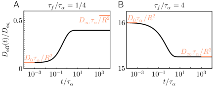
Figure 2: Effective diffusion coefficient of a condensate in a viscoelastic medium, $D_{\text{eff}}(t)\coloneqq\partial_{t}\operatorname{MSD}(t)$, relative to thermal equilibrium, $D_{\text{eq}}\coloneqq 6k_{B}T/(5\pi\eta R)$, for $\gamma\approx 0$. Solid lines indicate numerical solution of Eq. (9), red lines indicate (approximate) asymptotic limits [Eqs. (10) and (11)]. In both panels, the Péclet number is $\text{Pe}=D_{\text{eq}}\tau_{\alpha}/R^{2}=100$. A) For $\tau_{\alpha}>\tau_{f}>0$, condensate motion is suppressed compared to thermal equilibrium. The approximation for $D_{\infty}$ is worse for larger $\tau_{f}/\tau_{\alpha}$ where the decay of $\exp[-q^{2}\operatorname{MSD}(t)/6]$ in Eq. (9) is not mainly set by the early dynamics of $\operatorname{MSD}(t)$. B) For $\tau_{\alpha}<\tau_{f}$, condensate motion is enhanced relative to thermal equilibrium. The diffusivity depends only weakly on the timescale.

IV.4 Condensates in an active Maxwell fluid

The theory discussed so far is independent of the material properties of the condensate and the solvent. We will now apply this framework to a specific model system. To this end, we characterize the hydrodynamic fluctuations encoded in the correlation function $\mathcal{C}_{f}$. We consider an incompressible viscoelastic fluid with hydrodynamic screening borrowed from the Brinkman model [56]. The corresponding balance of forces reads

$$\bm{\nabla}\cdot\bm{\sigma}-\bm{\nabla}p-\eta\gamma\bm{v}_{f}+[\bm{\nabla}\cdot\bm{\alpha}-c\bm{\nabla}\mu]=0\,.$$ (12)

The pressure $p$ enforces incompressibility, $\bm{\nabla}\cdot\bm{v}_{f}=0$ similar to how the chemical potential $\mu$ enforces droplet cohesion in Eq. (1). We incorporate viscoelastic effects through the Maxwell model, $\tau_{f}\partial_{t}\bm{\sigma}+\bm{\sigma}=\eta\,[\bm{\nabla}\otimes\bm{v}_{f}+(\bm{\nabla}\otimes\bm{v}_{f})^{T}]$, with viscosity $\eta$ and elastic relaxation time $\tau_{f}$. For this model, the following Fourier-transformed Green’s function,

$$\widehat{\mathcal{G}}(\bm{q},\omega)=\frac{1}{\eta}\left[\frac{q^{2}}{1+i\tau_{f}\omega}+\gamma\right]^{-1}\left[\bm{I}-\frac{\bm{q}\otimes\bm{q}}{q^{2}}\right]\,,$$ (13)

relates applied forces and the resulting fluid flows. Although we have made the specific choice of a Maxwell fluid in the present manuscript, in general one can use the same framework to study other complex fluids or even solids such as the Kelvin-Voigt model.

Fluid flows are driven by the random stress tensor $\bm{\alpha}$ which can have passive and active parts. To interpolate between thermal-like and active stresses, we consider a random stress tensor with exponential memory,

$$\langle\alpha_{ij}(\bm{x},t)\alpha_{kl}(\bm{x}^{\prime},t^{\prime})\rangle=\frac{k_{B}T\eta}{\tau_{\alpha}}\,e^{-\frac{|t-t^{\prime}|}{\tau_{\alpha}}}\,\delta(\bm{x}-\bm{x}^{\prime})\color[rgb]{.5,.5,.5}\times\color[rgb]{0,0,0}\\ \color[rgb]{.5,.5,.5}\times\color[rgb]{0,0,0}\left[\delta_{ik}\delta_{jl}+\delta_{il}\delta_{jk}-\frac{2}{d}\delta_{ij}\delta_{kl}\right]\,.$$ (14)

In the limit $\tau_{\alpha}\to 0$, this converges to the fluctuating hydrodynamic stresses expected in a Stokes fluid [57], $\tau_{f}\to 0$. From the perspective of the generalized Langevin equation, the scenario $\tau_{\alpha}=\tau_{f}$ satisfies the fluctuation-dissipation theorem [58] and thus corresponds to thermal equilibrium. Therefore, we now have a handle on tuning the nonequilibrium dynamics of the viscoelastic fluid and the embedded condensate.

In the following, we make the approximation that the condensates do not significantly perturb the fluid flow. Relaxing this approximation [Appendix C] would allow us to calculate fluctuation-induced interactions between condensates, which is reserved for future work. The linear response [Eq. (13)] to the active stress fluctuations [Eq. (14)] predicts that the fluctuations in the viscoelastic fluid are characterized by

$$\frac{\eta\,\widehat{\mathcal{C}}_{f}(\bm{q},\omega)}{k_{B}T}=\frac{2(d-1)\,q^{2}}{(q^{2}+\gamma)^{2}+\gamma^{2}\tau_{f}^{2}\omega^{2}}\frac{1+\tau_{f}^{2}\omega^{2}}{1+\tau_{\alpha}^{2}\omega^{2}}\,.$$ (15)

Note that for spatially uncorrelated active forces with exponential memory, as opposed to active stresses [Eq. (14)], this expression would be modified by dividing by $q^{2}$. In this case, Eq. (9) predicts that the growth rate of the mean squared displacement would, on short timescales, diverge as $\propto\gamma^{-2+d/2}$. Physically, this implies that, in the absence of hydrodynamic screening, spherical condensates are in $d<4$ dimensions always unstable with respect to active forces, leading to either condensate splitting or shape fluctuations.

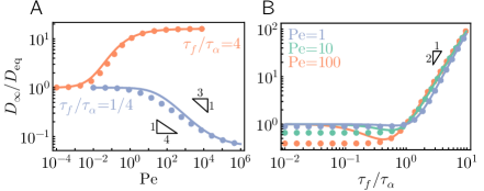
Figure 3: Diffusion coefficient of condensates on long timescales, relative to thermal equilibrium ($\tau_{f}=\tau_{\alpha}$), as a function of A) the Péclet number $\text{Pe}\coloneqq 6k_{B}T\tau_{\alpha}/(5\pi\eta R^{3})$ and B) the ratio between the fluid relaxation time $\tau_{f}$ and the stress correlation time $\tau_{\alpha}$. Solid lines represent analytical approximations, dots represent numerical calculations. For simplicity, we have neglected hydrodynamic screening, $\gamma\approx 0$.

IV.5 Active stirring can enhance or suppress motion

To make concrete predictions, we will now specialize the theory to spherical condensates with radius $R$ in $d=3$ dimensions. Henceforth, we will consider a simplified scenario where the screening length is large compared to the condensate size, $\sqrt{\gamma}R\ll 1$, on sufficiently long timescales so that $\gamma R^{2}\tau_{f}/t\ll 1$. With these approximations, the flow correlations of the viscoelastic fluid [Eq. (15)] can be simplified to

$$\frac{\eta\,\widehat{\mathcal{C}}_{f}(\bm{q},\omega)}{k_{B}T}\approx\frac{4\,q^{2}}{q^{4}+2\gamma q^{2}}\frac{1+\tau_{f}^{2}\omega^{2}}{1+\tau_{\alpha}^{2}\omega^{2}}\,.$$ (16)

For $\tau_{\alpha}=\tau_{f}$, which satisfies the fluctuation-dissipation theorem, the last term in Eq. (16) vanishes. Hence, there can only be a difference in condensate motion between short and long timescales, $D_{0}\neq D_{\infty}$, if $\tau_{\alpha}\neq\tau_{f}$. Figure 2 shows the slope of the mean squared displacement for two scenarios, $\tau_{\alpha}<\tau_{f}$ and $\tau_{\alpha}>\tau_{f}$.

Initially, the mean squared displacement of the condensate grows with the effective diffusion coefficient [Eq. (10)]

$$D_{0}\approx D_{c}+\frac{6k_{B}T}{5\pi\eta R}\frac{\tau_{f}^{2}}{\tau_{\alpha}^{2}}\left[1-\frac{5\sqrt{\gamma}R}{3\sqrt{2}}\right]\,,$$ (17)

to lowest order in $\sqrt{\gamma}R$. For small condensates, $R<$35\text{\,}\mathrm{nm}$$ estimated in Appendix G, motion is dominated by $D_{c}\propto 1/R^{3}$, and is independent of fluctuations in the viscoelastic fluid. Since one can assume that the condensates exceed this threshold size in practice, in the following we make the approximation $D_{c}\approx 0$. For large condensates, taking into account fluid stresses recovers the size dependence of the Stokes-Einstein relation, $D_{0}\propto 1/R$, in agreement with recent Cahn-Hilliard-Navier-Stokes simulations [59]. Compared to a solid object, the hydrodynamic radius of liquid biomolecular condensates is reduced by the factor $5/36$. Importantly, shorter stress correlation times $\tau_{\alpha}$, or longer fluid relaxation times $\tau_{f}$, amplify the Brownian motion of condensates relative to thermal equilibrium $\tau_{\alpha}=\tau_{f}$.

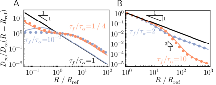
Figure 4: Effective diffusion coefficient of a condensate with radius $R$, compared to a reference condensate with radius $R_{\text{ref}}$. Solid lines indicate analytical approximations, dots represent numerical calculations for $\text{Pe}=1000$. A) For $\tau_{f}<\tau_{\alpha}$, there is a crossover regime where the diffusion coefficient is largely independent of condensate radius. Note that the analytical approximation fails when $\tau_{f}\ll\tau_{\alpha}$. B) For $\tau_{f}>\tau_{\alpha}$, there is a crossover regime where the diffusion coefficient departs from the Stokes-Einstein scaling. The width of this crossover regime increases with $\tau_{f}/\tau_{\alpha}$. We have here neglected hydrodynamic screening, $\gamma\approx 0$.

Next, we analyze the fluctuations of the center of mass of the condensate on long timescales [Eq. (11)], to lowest order in $\sqrt{\gamma}R$. For large condensates, $R\gg\sqrt{D_{0}\tau_{\alpha}}$, one approximately has

$$D_{\infty}\approx D_{0}+\frac{6k_{B}T}{5\pi\eta R}\left[1-\frac{\tau_{f}^{2}}{\tau_{\alpha}^{2}}\right]\left[1-\frac{5\sqrt{\gamma}R}{3\sqrt{2}}\right]\,.$$ (18)

Substituting Eq. (17) into Eq. (18) eliminates the dependence on $\tau_{f}/\tau_{\alpha}$, thus suggesting that large condensates show thermal-like dynamics on long timescales. In summary, for longer stress correlation times $\tau_{\alpha}$ or shorter fluid relaxation times $\tau_{f}$, condensate motion on long timescales ($D_{\infty}$) is faster than condensate motion on short timescales ($D_{0}$). This prediction is corroborated by Fig. 2, where we have solved Eq. (9) numerically for $\gamma\approx 0$ and by Fig. 3 where we compare the numerical results with analytical approximations.

For sufficiently small condensates, $R\ll\sqrt{D_{0}\tau_{\alpha}}$, the scaling of the effective diffusion coefficient with condensate size changes qualitatively. The analytical approximation,

$$D_{\infty}\approx D_{0}+\frac{\sqrt{6}k_{B}T}{\pi\eta\sqrt{D_{0}\tau_{\alpha}}}\left[1-\frac{\tau_{f}^{2}}{\tau_{\alpha}^{2}}\right]\left[1-\sqrt{\frac{\gamma D_{0}\tau_{\alpha}}{3}}\right]\,,$$ (19)

suggests a potential nonmonotonicity as a function of $D_{0}$ and thus condensate radius if $\tau_{\alpha}>\tau_{f}$. Our numerical calculations clarify that, instead of nonmonotonicity, there is a wide range of condensate sizes where the diffusion coefficient on long timescales, $D_{\infty}$, is actually insensitive to the condensate radius (Fig. 4A). Hence, active stirring of the viscoelastic medium has a qualitative effect on the Brownian motion of condensates with potentially far-reaching implications for coalescence—in addition to the motion-induced dipole interactions discussed above.

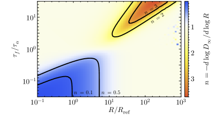
Figure 5: Scaling of the effective diffusion coefficient with condensate radius, $D_{\infty}\sim 1/R^{n}$. In the blue region of the phase diagram, condensate motion is almost independent of condensate size. In the red region of the phase diagram, the dependence of motion on condensate size is amplified. In all other regions (bright yellow), the Stokes-Einstein relation $D_{\infty}\sim 1/R$ holds.

When the effective diffusion coefficient $D_{\infty}$ is independent of the size of the condensates due to active fluctuations with $\tau_{\alpha}>\tau_{f}$ (Fig. 5), the average condensate radius has an increased scaling exponent $\langle R\rangle\sim t^{1/2}$ as a function of time. As the condensates grow in size, the effective diffusion coefficient recovers its size dependence $D_{\infty}\propto 1/R$ so that further growth follows the standard $\langle R\rangle\sim t^{1/3}$ scaling. In contrast, for $\tau_{\alpha}<\tau_{f}$, the effective diffusion coefficient scales over a wide range of condensate sizes as $D_{\infty}\propto 1/R^{n}$ with $n>1$ (Fig. 4B, Fig. 5), leading to a reduced scaling exponent $\langle R\rangle\sim t^{1/(2+n)}$. We expect that the rate of coalescence will initially be higher for $\tau_{\alpha}<\tau_{f}$ due to a larger effective diffusion coefficient $D_{\infty}$ which increases the rate of collisions (Fig. 3B). With increasing condensate radius, Brownian motion will be rapidly suppressed (Fig. 4B), thereby creating a bottleneck and skewing the droplet size distribution. These arguments neglect the fact that moving condensates show dipole-dipole interactions, which could further accelerate coalescence and will be investigated in future work.

V Discussion

In summary, we developed a framework for studying the Brownian motion of biomolecular condensates in actively driven viscoelastic environments. We have introduced active stress fluctuations by breaking the fluctuation dissipation theorem and have discovered that, in doing so, condensate motion can be either enhanced or suppressed. The theory predicts how condensate motion can be uncoupled from condensate size, thereby lifting a fundamental limitation on the frequency of collisions in polydisperse solutions. This could potentially find applications in the development of chemical reactors.

It would also be interesting to compare the predictions of the analytical theory with experiments. For example, recent work has shown that cytoskeletal activity quantitatively increases the frequency of collisions between biologically relevant condensates in the cell nucleus, such as speckles, leading to accelerated coalescence [32]. To interrogate this system further, one could tune the correlation time $\tau_{\alpha}$ of the active stress fluctuations by changing the residence time of molecular motors, or the relaxation time of the viscoelastic fluid $\tau_{f}$ by tuning the turnover of actin or actin crosslinkers. In addition, tracking the mean squared displacement and size distribution of condensates over time would yield complementary information. This would allow testing whether cells typically operate in the $\tau_{\alpha}>\tau_{f}$ or in the $\tau_{\alpha}>\tau_{f}$ regime and open new avenues for controlling intracellular organization.

Appendix A Derivation of force-velocity relation

First, we determine the chemical potential profile by solving the continuity equation, Eq. (1), using a traveling wave ansatz, $c(\bm{x},t)=c(\bm{z})$ with $\bm{z}\coloneqq\bm{x}-\bm{v}t$. For a condensate moving with velocity $\bm{v}$, this leads to the following chemical potential:

$$\mu(\bm{z})=-\Psi(\bm{z})+\frac{\Delta c}{M}\,\bm{v}\cdot\int_{\mathcal{D}}d^{d}\bm{z}^{\prime}\,\bm{\nabla}\mathcal{L}(\bm{z}-\bm{z}^{\prime})\\ -\frac{1}{M}\int d^{d}\bm{z}^{\prime}\,\bm{j}(\bm{z}^{\prime})\cdot\bm{\nabla}\mathcal{L}(\bm{z}-\bm{z}^{\prime})\,,$$ (20)

where we have defined the fundamental solution $\mathcal{L}(\bm{z})$ to the Laplace equation $\bm{\nabla}^{2}\mathcal{L}(\bm{z})=-\delta(\bm{z})$. Note that $\bm{\nabla}\equiv\bm{\nabla}_{\bm{z}}$ refers to the gradient with respect to the first argument and that $\mathcal{D}$ without time dependence is the condensate domain in the comoving and corotating frame. The gradient of the chemical potential in the co-moving and co-rotating frame is given by

$$\bm{\nabla}\mu(\bm{z})=-\bm{\nabla}\Psi(\bm{z})+\frac{\Delta c}{M}\,\mathcal{B}(\bm{z})\cdot\bm{v}\\ -\frac{1}{M}\,\int d^{d}\bm{z}^{\prime}\,\left[\bm{\nabla}\otimes\bm{\nabla}\mathcal{L}(\bm{z}-\bm{z}^{\prime})\right]\cdot\bm{j}(\bm{z}^{\prime})\,,$$ (21)

where we have defined the coupling tensor

$$\mathcal{B}(\bm{z})\equiv\mathcal{B}(\bm{z}|\mathcal{D})\coloneqq\bm{\nabla}\otimes\bm{\nabla}\int_{\mathcal{D}}d^{d}\bm{z}^{\prime}\,\mathcal{L}(\bm{z}-\bm{z}^{\prime})\,.$$ (22)

For spherical condensates with radius $R$, the integral can be evaluated:

$$\mathcal{B}(\bm{z})=-\begin{cases}\frac{\bm{I}}{d}\,,&|\bm{z}|\leq R\,,\\ \left[\frac{\bm{I}}{d}-\hat{\bm{z}}\otimes\hat{\bm{z}}\right](|\bm{z}|/R)^{-d}\,,&|\bm{z}|>R\,.\end{cases}$$ (23)

In essence, this is identical to the Green’s tensor for a dipolar electrostatic field. Transforming Eq. (21) into the laboratory frame, with shorthand notation $\bm{r}\equiv\bm{r}(t)$ for the position of the condensate moving with velocity $\bm{v}=\partial_{t}\bm{r}$, leads to Eq. (2) in the main text.

Using the thermodynamic consistency criterion [40],

$$\int_{\mathcal{D}}d^{d}\bm{z}\,\bm{\nabla}\mu(\bm{z})=0\,,$$ (24)

where $\mathcal{D}$ is the condensate domain in the co-moving and co-rotating frame, the chemical potential can be eliminated:

$$0=-\int_{\mathcal{D}}d^{d}\bm{z}\,M\bm{\nabla}\Psi(\bm{z})+\Delta c\,\int_{\mathcal{D}}d^{d}\bm{z}\,\mathcal{B}(\bm{z})\,\cdot\bm{v}\\ -\int d^{d}\bm{z}\,\mathcal{B}(\bm{z})\cdot\bm{j}(\bm{z})\,,$$ (25)

Next, we substitute Eq. (23). Note that the result for $\bm{z}\in\mathcal{D}$ can also be derived for general geometries by using isotropy, which implies $\mathcal{B}=\operatorname{tr}(\mathcal{B})\,\bm{I}/d$. Hence, without loss of generality, one has

$$\frac{\Delta cV_{\mathcal{D}}}{d}\,\bm{v}=-\int_{\mathcal{D}}d^{d}\bm{z}\,M\bm{\nabla}\Psi(\bm{z})-\int d^{d}\bm{z}\,\mathcal{B}(\bm{z})\cdot\,\bm{j}(\bm{z})\,.$$ (26)

where we have defined the condensate volume $V_{\mathcal{D}}\coloneqq\int_{\mathcal{D}}d^{d}\bm{z}$. The main insight here is that, in contrast to gradient flow dynamics, currents that cannot be represented by the gradient of a potential generically lead to nonlocal couplings.

Next, we substitute random thermal currents for the potential flux, $\bm{j}_{th}\coloneqq-M\bm{\nabla}\Psi$, and advection through the fluid for the nonpotential flux, $\bm{j}\coloneqq c\,\bm{v}_{f}$:

$$\frac{\Delta cV_{\mathcal{D}}}{d}\,\bm{v}=\int_{\mathcal{D}}d^{d}\bm{z}\,\bm{j}_{th}(\bm{z})-\int d^{d}\bm{z}\,c(\bm{z})\,\mathcal{B}(\bm{z})\cdot\bm{v}_{f}(\bm{z})\,.$$ (27)

Using $c(\bm{x},t)=c_{-}+\Delta c$ for $\bm{x}\in\mathcal{D}$, else $c_{-}$, to split the domain integral, leads to:

$$\frac{\Delta cV_{\mathcal{D}}}{d}\,\bm{v}=\int_{\mathcal{D}}d^{d}\bm{z}\,\bm{j}_{th}(\bm{z})-\Delta c\,\int_{\mathcal{D}}d^{d}\bm{z}\,\mathcal{B}(\bm{z})\cdot\bm{v}_{f}(\bm{z})\\ -c_{-}\,\int d^{d}\bm{z}\,\mathcal{B}(\bm{z})\cdot\bm{v}_{f}(\bm{z})\,,$$ (28)

To simplify the first line, we use Eq. (23). The second line can be eliminated via integration by parts and invoking fluid incompressibility, $\bm{\nabla}\cdot\bm{v}_{f}=0$:

$$\bm{v}=\frac{d}{\Delta c}\int_{\mathcal{D}}\frac{d^{d}\bm{z}}{V_{\mathcal{D}}}\,\bm{j}_{th}(\bm{z})+\int_{\mathcal{D}}\frac{d^{d}\bm{z}}{V_{\mathcal{D}}}\,\bm{v}_{f}(\bm{z})\,,$$ (29)

Note that the first term generalizes the result of Ref. [43] to arbitrary dimensions. The second term intuitively states that the condensate is advected by the average current of the fluid.

Appendix B Pairwise interactions between condensates

In this section, we will consider a generalized scenario in which two condensates interact through translation-induced polarization. We start from the premise that each condensate moves with the same velocity $\bm{v}$ when far away from other condensates. It does not matter how this motion is induced—potential mechanisms include phoresis, advection, or even optical trapping. What is important is that the motion of each condensate introduces a dipole force field. For example, consider the first condensate whose domain $\mathcal{D}_{1}$ is centered around $\bm{r}_{1}(t)$ and moves with velocity $\partial_{t}\bm{r}_{1}(t)\coloneqq\bm{v}+\delta\bm{v}_{1}$. Here, $\delta\bm{v}_{1}$ is the perturbation in which we are interested. According to Eq. (2), the motion of the condensate gives rise to an additive contribution to the chemical potential profile:

$$\bm{\nabla}\delta\mu_{1}(\bm{x},t)=\frac{\Delta c}{M}\,\mathcal{B}(\bm{x}-\bm{r}_{1}|\mathcal{D}_{1})\cdot[\bm{v}+\delta\bm{v}_{1}]\,,$$ (30)

where $\mathcal{B}(\bm{x}-\bm{r}_{1}|\mathcal{D}_{1})$ is given by Eq. (22). Using the same notation, we will now discuss the response of the second condensate.

The additional contribution to the chemical potential profile drives a potential flux. Consequently, the second condensate will move according to Eq. (26):

$$\delta\bm{v}_{2}=-\frac{d}{\Delta c}\int_{\mathcal{D}_{2}}\frac{d^{d}\bm{z}}{V_{\mathcal{D}_{2}}}\,M\bm{\nabla}\delta\mu_{1}(\bm{r}_{2}+\bm{z},t)\,.$$ (31)

Like before, $\mathcal{D}_{2}$ is the domain of the second condensate centered at $\bm{r}_{2}(t)$ and moving with velocity $\partial_{t}\bm{r}_{2}(t)\coloneqq\bm{v}+\delta\bm{v}_{2}$. Substituting Eq. (30) in Eq. (31) and using Eq. (22) leads to

$$\delta\bm{v}_{2}=\bm{M}_{21}\cdot[\bm{v}+\delta\bm{v}_{1}]\,,$$ (32)

where we have defined

$$\bm{M}_{21}=\frac{d}{V_{\mathcal{D}_{2}}}\oint_{\partial\mathcal{D}_{2}}\!\!d\bm{S}\,\otimes\,\oint_{\partial\mathcal{D}_{1}}\!\!d\bm{S}^{\prime}\,\mathcal{L}(\bm{r}_{2}-\bm{r}_{1}+\bm{z}-\bm{z}^{\prime})\,.$$ (33)

In the last step, we used Gauss’ theorem to simplify the integral. For small condensates that do not overlap, one can make the following approximation:

$$\bm{M}_{21}\approx-d\,V_{\mathcal{D}_{1}}\bm{\nabla}\otimes\bm{\nabla}\,\mathcal{L}(\bm{r}_{2}-\bm{r}_{1})\,.$$ (34)

The response of the first condensate to the motion of the second condensate is analogous, just with flipped indices $1\leftrightarrow 2$.

To understand under which conditions the two condensates will begin to approach or repel each other, we calculate $\partial_{t}(\bm{r}_{2}-\bm{r}_{1})$. Based on the above approximation for small condensate sizes, we assume that $\bm{M}_{21}$ and $\bm{M}_{12}$ commute. The separation between the two condensates will then gradually change according to

$$\delta\bm{v}_{2}-\delta\bm{v}_{1}\approx[\bm{I}-\bm{M}_{21}\cdot\bm{M}_{12}]^{-1}\cdot\left(\bm{M}_{21}-\bm{M}_{12}\right)\cdot\bm{v}\,.$$ (35)

For large separations between the condensates, the term in square brackets is approximately equal to the identity matrix. Thus, for large separations compared to the condensate size, one can further simplify:

$$\partial_{t}(\bm{r}_{2}-\bm{r}_{1})\approx d\left(V_{\mathcal{D}_{2}}-V_{\mathcal{D}_{1}}\right)\bm{\nabla}\otimes\bm{\nabla}\,\mathcal{L}(\bm{r}_{2}-\bm{r}_{1})\cdot\bm{v}\,.$$ (36)

where we have substituted Eq. (34). For spherical condensates in $d=3$ dimensions, one has $\mathcal{L}(\bm{z})=1/(4\pi|\bm{z}|)$ and $V_{\mathcal{D}_{1}}=4\pi/3\,R_{1}^{3}$, leading to

$$\partial_{t}(\bm{r}_{2}-\bm{r}_{1})\approx\left(R_{2}^{3}-R_{1}^{3}\right)\bm{\nabla}\otimes\bm{\nabla}\,\frac{1}{|\bm{r}_{2}-\bm{r}_{1}|}\cdot\bm{v}\,.$$ (37)

Appendix C Interdependence of fluid flow on condensates

We consider the dynamics of a viscoelastic fluid according to Eq. (12). Using the Green’s function, Eq. (13), the fluid flow is given by:

$$\bm{v}_{f}(\bm{x},t)=\int d^{d}\bm{x}^{\prime}\int_{-\infty}^{t}dt^{\prime}\,\mathcal{G}(\bm{x}-\bm{x}^{\prime},t-t^{\prime})\cdot\bm{f}(\bm{x}^{\prime},t^{\prime})\,,$$ (38)

with driving force $\bm{f}\coloneqq\bm{\nabla}\cdot\bm{\alpha}-c\bm{\nabla}\mu$. We split the flow into two contributions, $\bm{v}_{f}=\bm{v}_{f}^{\star}+\delta\bm{v}_{f}$, where

$$\bm{v}_{f}^{\star}(\bm{x},t)=\int d^{d}\bm{x}^{\prime}\int_{-\infty}^{t}\!\!dt^{\prime}\,\mathcal{G}(\bm{x}-\bm{x}^{\prime},t-t^{\prime})\cdot\bm{\nabla}\cdot\bm{\alpha}(\bm{x}^{\prime},t^{\prime})$$ (39)

arises from active and passive forces that are independent of the condensates, and

$$\delta\bm{v}_{f}(\bm{x},t)=-\int d^{d}\bm{x}^{\prime}\int_{-\infty}^{t}\!\!dt^{\prime}\,\mathcal{G}(\bm{x}-\bm{x}^{\prime},t-t^{\prime})\cdot c\bm{\nabla}\mu(\bm{x}^{\prime},t^{\prime})$$ (40)

models the perturbation of the fluid flow due to the presence of condensates. In the present section, we analyze the latter.

First, we use $c(\bm{x},t)=c_{-}+\Delta c$ for $\bm{x}\in\mathcal{D}(t)$, else $c_{-}$, to split the domain integral:

$$\delta\bm{v}_{f}(\bm{x},t)=-\int_{-\infty}^{t}\!\!dt^{\prime}\Biggl{[}\\ +c_{-}\int d^{d}\bm{x}^{\prime}\,\mathcal{G}(\bm{x}-\bm{x}^{\prime},t-t^{\prime})\cdot\bm{\nabla}\mu(\bm{x}^{\prime},t^{\prime})\\ +\Delta c\int_{\mathcal{D}(t^{\prime})}d^{d}\bm{x}^{\prime}\,\mathcal{G}(\bm{x}-\bm{x}^{\prime},t-t^{\prime})\cdot\bm{\nabla}\mu(\bm{x}^{\prime},t^{\prime})\Biggr{]}\,.$$ (41)

The second line can be eliminated via integration by parts, by using fluid incompressibility $\bm{\nabla}\cdot\mathcal{G}=0$ and the fact that the Green’s function decays to zero in the far field:

$$\delta\bm{v}_{f}(\bm{x},t)=-\Delta c\int_{-\infty}^{t}\!\!dt^{\prime}\color[rgb]{.75,.75,.75}\times\color[rgb]{0,0,0}\\ \color[rgb]{.75,.75,.75}\times\color[rgb]{0,0,0}\int_{\mathcal{D}(t^{\prime})}d^{d}\bm{x}^{\prime}\,\mathcal{G}(\bm{x}-\bm{x}^{\prime},t-t^{\prime})\cdot\bm{\nabla}\mu(\bm{x}^{\prime},t^{\prime})\,.$$ (42)

Now, we need to substitute the gradient of the chemical potential, Eq. (2), where we use $\bm{j}\coloneqq c\,\bm{v}_{f}$.

As before, we split the domain integral using $c(\bm{x},t)=c_{-}+\Delta c$ for $\bm{x}\in\mathcal{D}(t)$, else $c_{-}$. The term proportional to $c_{-}$ is eliminated via integration by parts, after replacing $\bm{\nabla}_{\bm{x}}\mathcal{L}(\bm{x}-\bm{x}^{\prime})=-\bm{\nabla}_{\bm{x}^{\prime}}\mathcal{L}(\bm{x}-\bm{x}^{\prime})$, by using fluid incompressibility and the fact that $\mathcal{L}$ decays to zero in the far field. Taken together, the chemical potential profile in the laboratory frame is given by:

$$\bm{\nabla}\mu(\bm{x},t)=-\bm{\nabla}\Psi(\bm{x},t)+\frac{\Delta c}{M}\,\mathcal{B}(\bm{x}-\bm{r})\cdot\bm{v}(t)\\ -\frac{\Delta c}{M}\,\int_{\mathcal{D}(t)}d^{d}\bm{x}^{\prime}\,\left[\bm{\nabla}\otimes\bm{\nabla}\mathcal{L}(\bm{x}-\bm{x}^{\prime})\right]\cdot\bm{v}_{f}(\bm{x}^{\prime},t)\,,$$ (43)

where $\bm{r}\equiv\bm{r}(t)$. This result illuminates that the effect of condensate motion on fluid flow is $\mathcal{O}(\Delta c^{2})$ and that it decays with the mobility of biomolecules, $\propto 1/M$. In the present manuscript, we neglect these higher-order corrections to the fluid flow. Nevertheless, we will briefly comment on how to make such corrections for spherical condensates with radius $R$, center of mass position $\bm{r}(t)\in\mathcal{D}(t)$ and velocity $\bm{v}\equiv\bm{v}(t)$.

In essence, in Eq. (42), we insert the chemical potential gradient generated by each condensate, Eq. (43). Here, the second term demonstrates how the motion of the condensate, with velocity $\bm{v}$, induces a force on the fluid, with the tensor $\mathcal{B}$ defined by Eq. (23). This result indicates that, in contrast to the motion of rigid inclusions, condensate motion induces long-range forces on the fluid. Substituting Eq. (43) into Eq. (42) results in

$$\delta\bm{v}_{f}(\bm{x},t)=\frac{\Delta c^{2}}{M}\int_{-\infty}^{t}\!\!dt^{\prime}\int_{\mathcal{D}(t^{\prime})}d^{d}\bm{x}^{\prime}\Biggl{\{}\\ +\mathcal{G}(\bm{x}-\bm{x}^{\prime},t-t^{\prime})\cdot\Biggl{[}\frac{\bm{v}(t^{\prime})}{d}+\frac{M\bm{\nabla}\Psi(\bm{x}^{\prime},t^{\prime})}{\Delta c}\Biggr{]}\\ +\mathcal{G}^{\prime}(\bm{x}-\bm{r}^{\prime},\bm{x}^{\prime}-\bm{r}^{\prime},t-t^{\prime})\cdot\bm{v}_{f}(\bm{x}^{\prime},t^{\prime})\Biggr{\}}\,,$$ (44)

where the time-dependent domain $\mathcal{D}(t^{\prime})$ of the droplet is centered around $\bm{r}^{\prime}\equiv\bm{r}(t^{\prime})$ and $\mathcal{B}(\bm{x}^{\prime}-\bm{r}^{\prime})=-\bm{I}/d$ for $|\bm{x}^{\prime}-\bm{r}^{\prime}|\leq R$. Moreover, we have defined

$$\mathcal{G}^{\prime}(\bm{x},\bm{x}^{\prime},t)\coloneqq\int_{\mathcal{D}}\!d^{d}\bm{z}\,\mathcal{G}(\bm{x}-\bm{z},t)\cdot\bm{\nabla}\otimes\bm{\nabla}\mathcal{L}(\bm{z}-\bm{x}^{\prime})\,,$$ (45)

where $\mathcal{D}$ is the time-independent domain of the condensate in the comoving and corotating frame. In future studies, these results can be used to derive an equivalent of the Rotne-Prager-Yamakawa tensor [60, 61] to study fluid-mediated interactions in the context of biomolecular condensates.

Appendix D Expansion of the fluid flow correlation function

To characterize the correlation of the fluid flow evaluated at randomly fluctuating locations, we consider a series expansion of the fluid flow field around the midpoint $\bar{\bm{r}}\coloneqq(\bm{r}+\bm{r}^{\prime})/2$ of the condensate trajectory in the time window $[t,t^{\prime}]$:

$$\bm{v}_{f}(\bm{z}+\bm{r},t)=\sum_{n}\frac{1}{n!}[(\bm{r}-\bar{\bm{r}})\cdot\bm{\nabla}_{\bm{z}}]^{n}\bm{v}_{f}(\bm{z}+\bar{\bm{r}},t)\,,$$ (46)

where $\bm{r}\equiv\bm{r}(t)$ and $\bm{r}^{\prime}\equiv\bm{r}(t^{\prime})$ are random variables corresponding to the condensate center of mass. The covariance of the fluid velocity is then given by:

$$\langle\bm{v}_{f}(\bm{z}+\bm{r},t)\cdot\bm{v}_{f}(\bm{z}^{\prime}+\bm{r}^{\prime},t^{\prime})\rangle=\sum_{nm}\frac{1}{n!m!}\Bigl{\langle}\left[\tfrac{\bm{r}-\bm{r}^{\prime}}{2}\cdot\bm{\nabla}_{\bm{z}}\right]^{n}\color[rgb]{.75,.75,.75}\times\color[rgb]{0,0,0}\\ \color[rgb]{.75,.75,.75}\times\color[rgb]{0,0,0}\left[\tfrac{\bm{r}^{\prime}-\bm{r}}{2}\cdot\bm{\nabla}_{\bm{z}^{\prime}}\right]^{m}\bm{v}_{f}(\bm{z}+\bar{\bm{r}},t)\cdot\bm{v}_{f}(\bm{z}^{\prime}+\bar{\bm{r}},t^{\prime})\Bigr{\rangle}\,,$$ (47)

where we have substituted the midpoint. Next, we will split the correlations of the condensate motion and the correlations of the fluid flow. To that end, we argue that the fluid flow fluctuates much faster than the condensate motion, so that one can make the preaveraging approximation $\bm{v}_{f}(\bm{z}+\bar{\bm{r}},t)\cdot\bm{v}_{f}(\bm{z}^{\prime}+\bar{\bm{r}},t^{\prime})\approx\langle\bm{v}_{f}(\bm{z}+\bar{\bm{r}},t)\cdot\bm{v}_{f}(\bm{z}^{\prime}+\bar{\bm{r}},t^{\prime})\rangle$. Another way to see this is from Eq. (6), which states that the fluid flow is averaged over the condensate size, so that condensate motion is almost independent of the fluid flow through an infinitesimally small region. After substituting the definition of the covariance of the hydrodynamic fluctuations, $\mathcal{C}_{f}(\bm{z}-\bm{z}^{\prime},t-t^{\prime})\coloneqq\langle\bm{v}_{f}(\bm{z},t)\cdot\bm{v}_{f}(\bm{z}^{\prime},t^{\prime})\rangle$, and using $\bm{\nabla}_{\bm{z}^{\prime}}\mathcal{C}_{f}(\bm{z}-\bm{z}^{\prime},t-t^{\prime})=-\bm{\nabla}_{\bm{z}}\mathcal{C}_{f}(\bm{z}-\bm{z}^{\prime},t-t^{\prime})$, one has:

$$\langle\bm{v}_{f}(\bm{z}+\bm{r},t)\cdot\bm{v}_{f}(\bm{z}^{\prime}+\bm{r}^{\prime},t^{\prime})\rangle\approx\sum_{nm}\frac{1}{n!m!}\color[rgb]{.75,.75,.75}\times\color[rgb]{0,0,0}\\ \color[rgb]{.75,.75,.75}\times\color[rgb]{0,0,0}\left\langle\left[\frac{\bm{r}-\bm{r}^{\prime}}{2}\cdot\bm{\nabla}_{\bm{z}}\right]^{n+m}\right\rangle\,\mathcal{C}_{f}(\bm{z}-\bm{z}^{\prime},t-t^{\prime})\,.$$ (48)

We continue our analysis by using Wick’s theorem:

$$\langle\bm{v}_{f}(\bm{z}+\bm{r},t)\cdot\bm{v}_{f}(\bm{z}^{\prime}+\bm{r}^{\prime},t^{\prime})\rangle\approx\sum_{\begin{subarray}{c}nm\\ n+m\text{ even}\end{subarray}}\frac{1}{n!m!}\frac{(n+m)!}{\left(\frac{n+m}{2}\right)!}\color[rgb]{.75,.75,.75}\times\color[rgb]{0,0,0}\\ \color[rgb]{.75,.75,.75}\times\color[rgb]{0,0,0}\frac{1}{2^{\frac{n+m}{2}}}\left\langle\left[\frac{\bm{r}-\bm{r}^{\prime}}{2}\cdot\bm{\nabla}_{\bm{z}}\right]^{2}\right\rangle^{\frac{n+m}{2}}\,\mathcal{C}_{f}(\bm{z}-\bm{z}^{\prime},t-t^{\prime})\,.$$ (49)

Next, we define the integer $l=\frac{n+m}{2}$ to reorder the summation and exploit isotropy, $\langle\Delta\bm{r}\otimes\Delta\bm{r}\rangle=\langle|\Delta\bm{r}|^{2}\rangle\,\bm{I}/d$, leading to:

$$\langle\bm{v}_{f}(\bm{z}+\bm{r},t)\cdot\bm{v}_{f}(\bm{z}^{\prime}+\bm{r}^{\prime},t^{\prime})\rangle\approx\sum_{l}\sum_{n=0}^{2l}\frac{(2l)!}{n!(2l-n)!}\color[rgb]{.75,.75,.75}\times\color[rgb]{0,0,0}\\ \color[rgb]{.75,.75,.75}\times\color[rgb]{0,0,0}\frac{1}{l!}\frac{1}{2^{l}}\left[\frac{1}{4d}\left\langle[\bm{r}-\bm{r}^{\prime}]^{2}\right\rangle\bm{\nabla}_{\bm{z}}^{2}\right]^{l}\,\mathcal{C}_{f}(\bm{z}-\bm{z}^{\prime},t-t^{\prime})\,.$$ (50)

Finally, after evaluating the inner sum, one arrives at the equation in the main text:

$$\langle\bm{v}_{f}(\bm{z}+\bm{r},t)\cdot\bm{v}_{f}(\bm{z}^{\prime}+\bm{r}^{\prime},t^{\prime})\rangle\\ \approx\sum_{l}\frac{1}{l!}\left[\frac{1}{2d}\left\langle[\bm{r}-\bm{r}^{\prime}]^{2}\right\rangle\bm{\nabla}_{\bm{z}}^{2}\right]^{l}\,\mathcal{C}_{f}(\bm{z}-\bm{z}^{\prime},t-t^{\prime})\\ =\exp\biggl{[}\frac{1}{2d}\left\langle[\bm{r}-\bm{r}^{\prime}]^{2}\right\rangle\bm{\nabla}_{\bm{z}}^{2}\biggr{]}\,\mathcal{C}_{f}(\bm{z}-\bm{z}^{\prime},t-t^{\prime})\,.$$ (51)

Appendix E Differential equation for mean-squared displacement

Substituting Eq. (8) into Eq. (7) leads to

$$\langle\bm{v}(t)\cdot\bm{v}(t^{\prime})\rangle=D_{c}\,\delta(t-t^{\prime})+\iint_{\mathcal{D}}\frac{d^{d}\bm{z}}{V_{\mathcal{D}}}\frac{d^{d}\bm{z}^{\prime}}{V_{\mathcal{D}}}\,\color[rgb]{.75,.75,.75}\times\color[rgb]{0,0,0}\\ \color[rgb]{.75,.75,.75}\times\color[rgb]{0,0,0}\exp\biggl{[}\frac{1}{2d}\left\langle[\bm{r}(t)-\bm{r}(t^{\prime})]^{2}\right\rangle\bm{\nabla}_{\bm{z}}^{2}\biggr{]}\,\mathcal{C}_{f}(\bm{z}-\bm{z}^{\prime},t-t^{\prime})\,.$$ (52)

Next, we use the identity $\partial_{t}\partial_{t^{\prime}}\langle|\bm{r}(t)-\bm{r}(t^{\prime})|^{2}\rangle=-2\langle\bm{v}(t)\cdot\bm{v}(t^{\prime})\rangle$ and define the mean squared displacement, $\operatorname{MSD}(t-t^{\prime})\coloneqq\langle|\bm{r}(t)-\bm{r}(t^{\prime})|^{2}\rangle$, to arrive at the following nonlinear differential equation:

$$\frac{1}{2}\partial_{t}^{2}\operatorname{MSD}(t)=D_{c}\,\delta(t)+\iint_{\mathcal{D}}\frac{d^{d}\bm{z}}{V_{\mathcal{D}}}\frac{d^{d}\bm{z}^{\prime}}{V_{\mathcal{D}}}\,\color[rgb]{.75,.75,.75}\times\color[rgb]{0,0,0}\\ \color[rgb]{.75,.75,.75}\times\color[rgb]{0,0,0}\exp\biggl{[}\frac{1}{2d}\operatorname{MSD}(t)\bm{\nabla}_{\bm{z}}^{2}\biggr{]}\,\mathcal{C}_{f}(\bm{z}-\bm{z}^{\prime},t)\,.$$ (53)

In the following, we will consider spherical condensates with radius $R$. In this case, the differential equation Eq. (53) can be cast into a numerically more convenient form via a Fourier transform in space and time,

$$\widehat{\mathcal{C}}_{f}(|\bm{q}|,\omega) \coloneqq\int d^{d}\bm{z}\int dt\,e^{-i\bm{q}\cdot\bm{z}-i\omega t}\,\mathcal{C}_{f}(\bm{z},t)\,,$$ (54)

$$\mathcal{C}_{f}(\bm{z},t) \coloneqq\int\frac{d^{d}\bm{q}}{(2\pi)^{d}}\int\frac{d\omega}{2\pi}\,e^{i\bm{q}\cdot\bm{z}+i\omega t}\,\widehat{\mathcal{C}}_{f}(|\bm{q}|,\omega)\,,$$ (55)

where we have taken into account the isotropy of the correlation function. This leads to the following equation:

$$\frac{1}{2}\partial_{t}^{2}\operatorname{MSD}(t)=D_{c}\,\delta(t)+\frac{d\,\Gamma\bigl{(}1+\tfrac{d}{2}\bigr{)}}{\pi^{d/2}R^{d}}\int\frac{d\omega}{2\pi}e^{i\omega t}\,\color[rgb]{.75,.75,.75}\times\color[rgb]{0,0,0}\\ \color[rgb]{.75,.75,.75}\times\color[rgb]{0,0,0}\int_{0}^{\infty}\!\frac{dq}{q}\,\exp\biggl{[}-\frac{q^{2}}{2d}\operatorname{MSD}(t)\biggr{]}\,J_{d/2}^{2}(qR)\,\widehat{\mathcal{C}}_{f}(q,\omega)\,,$$ (56)

with the form factor given by the Bessel function of the first kind,

$$J_{d/2}(q)=\frac{q^{d/2}}{2^{d/2}\Gamma\bigl{(}1+\tfrac{d}{2}\bigr{)}}\int_{|\bm{x}|\leq 1}\frac{d^{d}\bm{x}}{V_{1}}e^{i\bm{q}\cdot\bm{x}}\,,$$ (57)

where $V_{1}$ is the volume of the 1-sphere.

Importantly, if the high-frequency modes of the fluid flow do not decay to zero

$$\widehat{\mathcal{C}}_{f}(q,\infty)\coloneqq\lim_{\omega\to\infty}\widehat{\mathcal{C}}_{f}(q,\omega)\neq 0\,,$$ (58)

then this will lead to an additional $\delta$-correlated contribution to the transformed differential equation, Eq. (56). Hence, we split the correlation function of the fluid flow,

$$\widehat{\mathcal{C}}_{f}(q,\omega)=\widehat{\mathcal{C}}_{f}(q,\infty)+\left[\widehat{\mathcal{C}}_{f}(q,\omega)-\widehat{\mathcal{C}}_{f}(q,\infty)\right]\,,$$ (59)

and use the trivial initial condition $\operatorname{MSD}(0)=0$ to rewrite the differential equation, Eq. (56):

$$\frac{1}{2}\partial_{t}^{2}\operatorname{MSD}(t)=D_{c}\,\delta(t)\\ +\frac{d\,\Gamma\bigl{(}1+\tfrac{d}{2}\bigr{)}}{\pi^{d/2}R^{d}}\int_{0}^{\infty}\!\frac{dq}{q}\,J_{d/2}^{2}(qR)\,\widehat{\mathcal{C}}_{f}(q,\infty)\,\delta(t)\\ +\frac{d\,\Gamma\bigl{(}1+\tfrac{d}{2}\bigr{)}}{\pi^{d/2}R^{d}}\int\frac{d\omega}{2\pi}e^{i\omega t}\,\int_{0}^{\infty}\!\frac{dq}{q}\exp\biggl{[}-\frac{q^{2}}{2d}\operatorname{MSD}(t)\biggr{]}\color[rgb]{.75,.75,.75}\times\color[rgb]{0,0,0}\\ \color[rgb]{.75,.75,.75}\times\color[rgb]{0,0,0}J_{d/2}^{2}(qR)\,\left[\widehat{\mathcal{C}}_{f}(q,\omega)-\widehat{\mathcal{C}}_{f}(q,\infty)\right]\,.$$ (60)

Note that the mean squared displacement is a symmetric function under time reversal. By integrating Eq. (60) within an infinitesimally small region around the origin, one can now derive the second initial condition, $\partial_{t}\operatorname{MSD}(0^{+})=D_{0}$, where

$$D_{0}=D_{c}+\frac{d\,\Gamma\bigl{(}1+\tfrac{d}{2}\bigr{)}}{\pi^{d/2}R^{d}}\int_{0}^{\infty}\!\frac{dq}{q}\,J_{d/2}^{2}(qR)\,\widehat{\mathcal{C}}_{f}(q,\infty)\,.$$ (61)

For $t>0$, where the $\delta$-distributions vanish, one has:

$$\frac{1}{2}\partial_{t}^{2}\operatorname{MSD}(t)=\frac{d\,\Gamma\bigl{(}1+\tfrac{d}{2}\bigr{)}}{\pi^{d/2}R^{d}}\int_{0}^{\infty}\!\frac{dq}{q}\exp\biggl{[}-\frac{q^{2}}{2d}\operatorname{MSD}(t)\biggr{]}\color[rgb]{.75,.75,.75}\times\color[rgb]{0,0,0}\\ \color[rgb]{.75,.75,.75}\times\color[rgb]{0,0,0}J_{d/2}^{2}(qR)\,\int\!\frac{d\omega}{2\pi}e^{i\omega t}\left[\widehat{\mathcal{C}}_{f}(q,\omega)-\widehat{\mathcal{C}}_{f}(q,\infty)\right]\,.$$ (62)

Note that since the $\delta$-distributions do not matter for $t>0$, one can also drop the corresponding terms in Eqs. (62) and (53), leading to the expression reported in the main text [Eq. (9)].

Appendix F Asymptotic limits: short and long timescale dynamics

The dynamics on short timescales are dominated by the initial condition on the slope of the mean squared displacement, $\partial_{t}\operatorname{MSD}(0^{+})=D_{0}$, with the effective diffusion coefficient Eq. (10). Hence, the mean squared displacement grows linearly with time, $\operatorname{MSD}(t)\approx D_{0}|t|$.

To understand the dynamics on long timescales, we integrate Eq. (56) forward in time:

$$\partial_{t}\operatorname{MSD}(t)=2\int_{0}^{t}dt^{\prime}\Biggl{[}D_{c}\,\delta(t^{\prime})+\frac{d\,\Gamma\bigl{(}1+\tfrac{d}{2}\bigr{)}}{\pi^{d/2}R^{d}}\int\frac{d\omega}{2\pi}e^{i\omega t^{\prime}}\color[rgb]{.75,.75,.75}\times\color[rgb]{0,0,0}\\ \color[rgb]{.75,.75,.75}\times\color[rgb]{0,0,0}\int_{0}^{\infty}\!\frac{dq}{q}\,\exp\biggl{[}-\frac{q^{2}}{2d}\operatorname{MSD}(t^{\prime})\biggr{]}\,J_{d/2}^{2}(qR)\,\widehat{\mathcal{C}}_{f}(q,\omega)\Biggr{]}\,.$$ (63)

First, we symmetrize the integration domain, which is enabled by the time-reversal symmetry of the mean squared displacement. Moreover, we note that the exponential in the second line has its peak at $t^{\prime}=0$ and then monotonically decays. This decay is dominated by the dynamics on short timescales, where $\operatorname{MSD}(t)\approx D_{0}|t|$. Hence, the growth of the mean squared displacement on large timescales is governed by another effective diffusion coefficient:

$$D_{\infty}\approx D_{c}+\int_{-\infty}^{\infty}dt^{\prime}\frac{d\,\Gamma\bigl{(}1+\tfrac{d}{2}\bigr{)}}{\pi^{d/2}R^{d}}\int\frac{d\omega}{2\pi}e^{i\omega t^{\prime}}\color[rgb]{.75,.75,.75}\times\color[rgb]{0,0,0}\\ \color[rgb]{.75,.75,.75}\times\color[rgb]{0,0,0}\int_{0}^{\infty}\!\frac{dq}{q}\,\exp\biggl{[}-\frac{q^{2}}{2d}D_{0}|t^{\prime}|\biggr{]}\,J_{d/2}^{2}(qR)\,\widehat{\mathcal{C}}_{f}(q,\omega)\,,$$ (64)

where we have defined $D_{\infty}\coloneqq\lim_{t\to\infty}\partial_{t}\operatorname{MSD}(t)$. Splitting the correlation function of the fluid flow according to Eq. (59), and performing the Fourier transform, one finds:

$$D_{\infty}\approx D_{0}+\frac{d\,\Gamma\bigl{(}1+\tfrac{d}{2}\bigr{)}}{\pi^{d/2}R^{d}}\int_{0}^{\infty}\!\frac{dq}{q}\,J_{d/2}^{2}(qR)\,\color[rgb]{.75,.75,.75}\times\color[rgb]{0,0,0}\\ \color[rgb]{.75,.75,.75}\times\color[rgb]{0,0,0}\int\frac{d\omega}{2\pi}\frac{4dD_{0}q^{2}}{4d^{2}\omega^{2}+D_{0}^{2}q^{4}}\left[\widehat{\mathcal{C}}_{f}(q,\omega)-\widehat{\mathcal{C}}_{f}(q,\infty)\right]\,.$$ (65)

The second term determines whether condensate motion on large timescales is faster or slower than condensate motion on short timescales.

Appendix G Parameter estimation

For a spherical condensate in $d=3$ dimensions, the dimensionless ratio

$$\frac{6k_{B}T}{5\pi\eta R\,D_{c}}=\frac{2\Delta\phi^{2}R^{2}}{15a^{2}}\,,$$ (66)

determines which term in Eq. (17) is dominant. Here, we have used Stokes’ law, $M\nu=1/(6\pi\eta a)$, for the mobility of a molecule with radius $a\sim$2.5\text{\,}\mathrm{nm}$$ and molecular volume $\nu=\frac{4\pi}{3}a^{3}$, and defined the volume fraction difference $\Delta\phi\coloneqq\Delta c\,\nu$. Assuming a volume fraction difference of $\Delta\phi=0.2$, the second term in Eq. (17) will dominate if the condensate is larger than

$$R\gg\sqrt{\frac{15}{2}}\frac{a}{\Delta\phi}\sim$35\text{\,}\mathrm{nm}$\,.$$ (67)

For all practical purposes, this can be considered to always be the case. Otherwise, the condensate size would be on the length scale of the phase-separating molecules.

Appendix H Numerical calculations

This section details the numerical calculation of the mean squared displacement of spherical condensates with radius $R$ in $d=3$ dimensions. As discussed in the previous section, the first term in Eq. (17) is negligible for most practical scenarios. Hence, in the following, we make the approximation $D_{c}\approx 0$. Moreover, for simplicity, we also neglect hydrodynamic screening, $\gamma\approx 0$. With these simplifications, one has

$$D_{0}\approx\frac{6k_{B}T}{5\pi\eta R}\frac{\tau_{f}^{2}}{\tau_{\alpha}^{2}}\,,$$ (68)

which sets the initial condition $\partial_{t}\operatorname{MSD}(0^{+})=D_{0}$. The second initial condition, as discussed before, is given by $\text{MSD(0)}=0$. In the following, we define the ratio between the fluid relaxation time and the stirring time, $\Lambda\coloneqq\tau_{f}/\tau_{\alpha}$, and the Péclet number, $\text{Pe}\coloneqq\frac{6k_{B}T\tau_{\alpha}}{5\pi\eta R^{3}}$. For a condensate with radius $R=$100\text{\,}\mathrm{nm}$$, and a stirring time of $\tau_{\alpha}=$1\text{\,}\mathrm{s}$$, the Péclet number is $\text{Pe}\sim 1600$. For a condensate with radius $R=$1\text{\,}\mathrm{\SIUnitSymbolMicro m}$$, the Péclet number is $\text{Pe}\sim 1.6$. Finally, we define $s\coloneqq t/\tau_{\alpha}$ as the nondimensionalized time and $X(t)\coloneqq\operatorname{MSD}(t)/R^{2}$ as the nondimensionalized mean squared displacement.

To summarize, we solve the following nondimensionalized differential equation:

$$\frac{1}{2}\partial_{s}^{2}X=\frac{15}{4}\text{Pe}\,\left[1-\Lambda^{2}\right]e^{-s}K(X)\,,$$ (69)

where

$$K(X)\coloneqq\int_{0}^{\infty}\!\frac{dq}{q^{3}}\exp\biggl{[}-\frac{q^{2}}{6}X\biggr{]}J_{3/2}^{2}(q)\,.$$ (70)

The initial condition is

$$\partial_{s}X(0^{+})=\text{Pe}\,\Lambda^{2}\,,$$ (71)

and $X(0)=0$.

The asymptotic dynamics on short timescales are given by

$$\frac{D_{0}\tau_{\alpha}}{R^{2}}\approx\text{Pe}\,\Lambda^{2}\,,$$ (72)

and on long timescales are given by

$$\frac{D_{\infty}\tau_{\alpha}}{R^{2}}\approx\text{Pe}\,\Lambda^{2}\Biggl{[}1+45\frac{1-\Lambda^{2}}{\Lambda^{2}}\,\int_{0}^{\infty}\!\frac{dq}{q^{3}}\,\frac{J_{3/2}^{2}(q)}{6+\text{Pe}\,\Lambda^{2}q^{2}}\Biggr{]}\,.$$ (73)