E-LDA: Toward Interpretable LDA Topic Models with Strong Guarantees
in Logarithmic Parallel Time

Abstract

In this paper, we provide the first practical algorithms with provable guarantees for the problem of inferring the topics assigned to each document in an LDA topic model. This is the primary inference problem for many applications of topic models in social science, data exploration, and causal inference settings. We obtain this result by showing a novel non-gradient-based, combinatorial approach to estimating topic models. This yields algorithms that converge to near-optimal posterior probability in logarithmic parallel computation time (adaptivity)—exponentially faster than any known LDA algorithm. We also show that our approach can provide interpretability guarantees such that each learned topic is formally associated with a known keyword. Finally, we show that unlike alternatives, our approach can maintain the independence assumptions necessary to use the learned topic model for downstream causal inference methods that allow researchers to study topics as treatments. In terms of practical performance, our approach consistently returns solutions of higher semantic quality than solutions from state-of-the-art LDA algorithms, neural topic models, and LLM-based topic models across a diverse range of text datasets and evaluation parameters.

[name=Theorem, sibling=theorem]rThm [name=Lemma, sibling=theorem]rLem [name=Corollary, sibling=theorem]rCor

1 Introduction

Topic models such as Latent Dirichlet Allocation (LDA) (Blei et al., 2003) have become central to numerous high-profile streams of social science research ranging from the history of science to economics and political science (Ash and Hansen, 2023; Barberá et al., 2019; Bybee et al., 2024; Djourelova, 2023; Blanes i Vidal et al., 2012; Catalinac, 2016; Griffiths and Steyvers, 2004; Hall et al., 2008; Lauderdale and Clark, 2014; Martin and McCrain, 2019; Dietrich et al., 2019; Mueller and Rauh, 2018; Pan and Chen, 2018; Tingley, 2017). These models seek to learn the latent thematic structure that describes the content of a text dataset. Specifically, topic models posit that each document’s words were drawn from a (latent) document-specific mixture of (latent) topics, where each topic is a distribution over all words in a vocabulary.

For many applications of topic models, the primary goal is to estimate the set of latent topics, which provides a simple yet semantically rich summary of the data. In contrast, for the majority of applications in social science and data exploration, practitioners’ primary goal is to infer each document’s most probable assigned topics. These document-level topic assignments are then used as document labels that can be piped into downstream document-level regression analysis or causal inference methods.

Social scientists continue to strongly prefer LDA for this task over recent neural and LLM/BERT-based topic models for two reasons. First, social science research designs favor parametric models that are amenable to analysis. This is particularly important when using topic model outputs as labels for downstream models whose theoretic guarantees require that labels are well-estimated, consistent, conditionally independent, etc. Second, social scientists assume that the latent LDA topic space is semantically interpretable. However, there are three key challenges.

There are no known provable guarantees for the topic assignment problem. First, it is well-known that full posterior inference of LDA parameters is NP-hard even with just $2$ topics (Arora et al., 2012). Under various assumptions, it is possible to approximate LDA’s set of topics in poly-time (Anandkumar et al., 2012; Arora et al., 2012, 2013, 2016a, 2018). However, even if these latent topics are known, it is still NP-hard in general to learn LDA’s Maximum A Posteriori (MAP) assignments (i.e., which topic probably generated each word in a given document) (Sontag and Roy, 2011). Practitioners therefore resort to heuristic inference techniques such as variational inference (Blei et al., 2003) or Gibbs samplers (Griffiths and Steyvers, 2004). These approaches are well-motivated, but they seek only locally modal solutions and produce poorly fit results on some datasets (Gerlach et al., 2018).

Existing algorithms are generally incompatible with causal inference. Second, there has been much recent interest in causal inference frameworks that consider documents’ topics as treatments or outcomes (Egami et al., 2022; Feder et al., 2021, 2022; Fong and Grimmer, 2016, 2023; Hu and Li, 2021; Veitch et al., 2020). Obtaining documents’ topic assignments for these frameworks requires a 2nd round of inference using out-of-sample inference algorithms. However, out-of-sample algorithms also lack approximation guarantees, which undermines the usual guarantees for causal inference and yields spurious inferences with unbounded bias (Battaglia et al., 2024).

Existing algorithms learn and assign some uninterpretable topics. Finally, social scientists continue to prefer parametric topic models like LDA over neural and LLM-based models because they assume that the latent LDA topic space is interpretable. However, practitioners who wish to understand LDA results must manually parse topics that are arbitrary distributions over e.g. $20{,}000$ words in search of semantic meaning, then subjectively choose a topic ‘label’ (e.g. “this topic is about ‘physics’”)—a burdensome and subjective process that was famously compared to ‘reading tea leaves’ (Chang et al., 2009; Lau et al., 2014). In practice, researchers find that 10% of the topics learned by standard algorithms are fully nonsensical, and many more are partially nonsensical (Mimno et al., 2011). These problems have led to vast research on post-hoc evaluation of topics’ semantic quality and inspired recent excitement about algorithms that attempt to heuristically associate topics with keywords (Eshima et al., 2020; Doshi-Velez et al., 2015; Mimno et al., 2011; Röder et al., 2015). However, we lack a formal means to guarantee that each topic ascribes probability mass in an interpretable way, such as via a known function of a known keyword.

These various problems make LDA an outlier among related ML techniques. Seminal work of Blei et al. (2003) shows that LDA is a hierarchical extension of clustering (e.g. ‘mixture of unigrams’). Yet unlike LDA, clustering models have recently benefited from theoretic breakthroughs in combinatorial optimization that yielded fast algorithms with near-optimal approximation guarantees. These include exemplar-based problem formulations that convey additional interpretability advantages and other desirable properties (Breuer et al., 2020; Balkanski et al., 2019; Liu et al., 2013; Mirzasoleiman et al., 2013, 2015).

$\diamond\ \diamond\ \diamond$
Can the breakthroughs in optimization that recently revolutionized clustering algorithms also yield similarly fast, near-optimal, interpretable topic models? $\diamond\ \diamond\ \diamond$

Our contribution. We show the first practical algorithms that near-optimally solve the Maximum A Posteriori (MAP) topic-word assignment problem for LDA—that is, we provably obtain the near-optimal topic from which each word (and document) in the dataset was probably drawn.

We contrast our approach with standard LDA algorithms, which fix a small set of topics and use gradients to adjust them incrementally towards a local mode. That standard approach relies on hyperparameters to encourage a desirably sparse set of topics in document’s underlying distributions. Then, after fitting a model, practitioners typically compute topics’ coherence scores, prune low-coherence topics, and manually label topics with heuristic keywords.

We invert this approach to develop a combinatorial approach to estimating topic models. Suppose we have a very large ‘candidate set’ of topics from which the sparse set of topics in the solution are selected. It is easy to obtain this candidate set from other algorithms. Alternatively, we show we can simply initialize it to all feasible topics that meet standard interpretability criteria, so any topic selected for the solution will ascribe mass via a known function of some keyword. Then, instead of relying on gradients and heuristic sparsity-encouraging hyperparameters, we proceed combinatorially. Specifically, we consider the MAP assignment problem under an explicit sparsity constraint that upper-bounds the mean number of topics from which each document was drawn. This approach conveys multiple theoretic advantages for social science applications as we discuss below, and it brings LDA into line with recent techniques in clustering and data summarization.

Provable guarantees. Our algorithm obtains a deterministic worst-case $1$-$1/e$ approximation of the constrained log MAP probability objective (i.e. the most probable topic from which each word was drawn) in a number of iterations that is linear in the count of documents, where each iteration’s runtime is just logarithmic in the count of documents. We also give a parallel algorithm that converges w.p. in logarithmic iterations (adaptivity). This is exponentially faster than any known LDA algorithm. Because our algorithms can also perform out-of-sample inference, they also provide a means to use LDA for causal inference with provable approximation guarantees.

Practical performance. Finally, we show that our algorithms consistently learn solutions of higher semantic quality (coherence) than those found by state-of-the-art LDA algorithms, neural topic models, and LLM/BERT-based topic models. These improvements hold across a diverse set of text datasets and evaluation parameters.

Technical overview. From a purely technical perspective, there are four major challenges addressed in this work. The first is to show that under certain conditions, the classic LDA MAP assignment problem can be cast as a combinatorial optimization problem whose objective function exhibits the key diminishing returns property known as monotone submodularity. Submodularity is heavily studied in clustering, data summarization, and NLP problems, but surprisingly, its connection to topic models remained undiscovered (Gomes and Krause, 2010; Mirzasoleiman et al., 2015, 2016; Lin and Bilmes, 2011). Due to this property, the problem admits near-optimal solutions via generic Greedy algorithms (Nemhauser et al., 1978). Unfortunately, vanilla Greedy algorithms are practically infeasible for this objective because their runtime complexity scales as a third order polynomial in terms of the number of documents. In fact, because this objective is defined on sets of topic-to-document connections (links), not documents, solving it for even modest text corpora requires us to solve some of the largest combinatorial optimization problems considered in any academic research in terms of the sizes of the ground set (potential links) and solution set. Therefore, our second challenge is to design a fast serial algorithm for this problem with the same near-optimal Greedy approximation guarantee by leveraging the special independence structure of LDA’s probabilistic model. We then show that our techniques also apply to very recent parallel adaptive sampling algorithms (Balkanski and Singer, 2018; Breuer et al., 2020). We leverage this to obtain near-optimal MAP solutions w.h.p. in logarithmic parallel time.

Because our techniques are combinatorial, they permit the researcher to define the (possibly very large) ‘candidate set’ of topics from which the solution topics will be selected. This set can be obtained from existing algorithms, but this does not address the interpretability problems described above. Therefore, our third challenge is to show that it is possible to efficiently generate this candidate set of topics via standard coherence functions that are widely used to measure topics’ interpretive quality ex-post. Finally, our fourth challenge is to show that our techniques enforce document independences (SUTVA, etc.) required for downstream causal inference frameworks. This enables causal inference research designs on documents’ LDA topics that inherit near-optimal approximation guarantees.

2 LDA MAP topic-word assignment problem

The LDA model states that the data is a corpus (set) $D$ of documents and each document $d\in D$ is a multiset of words: $d=[w_{1},\dots,w_{|d|}]$. Suppose there are $k$ topics, where each topic is a distribution over all words in the vocabulary. LDA states that the text corpus is generated as follows: For each document $d$, we sample a document length $|d|$ and a document mixture distribution $\theta_{d}\sim Dirichlet(\alpha)$ over the $k$ topics. Then, to draw each of the $|d|$ words in $d$, we sample a topic $z_{d,i}\in\{1,\dots,k\}$, where $z_{d,i}\sim Categorical(\theta_{d})$, and from this topic we sample a word $w_{d,i}\sim Categorical(\phi_{z_{d,i}})$, where $\phi_{z}$ is the distribution over all words corresponding to topic $z$.

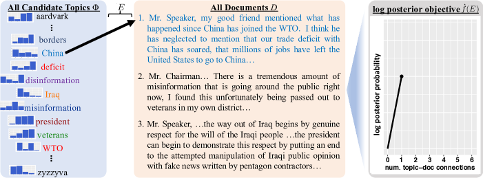
(a) Top: Objective $\dot{f}$ after 1 Greedy iteration. Note that $1$ topic-to-document link was added to solution set $E$.

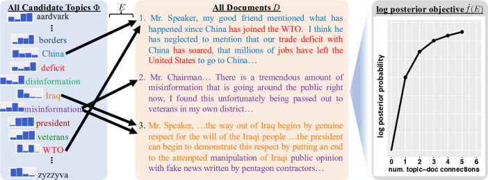
(b) Bottom: $\dot{f}$ after 5 iterations. Each word is (re-)assigned (see colors) to its most likely topic of those linked to its document per eq. 2.

Figure 1: Illustration of E-LDA approach to topic modeling. Note submodular ‘diminishing returns’ in $\dot{f}$.

We refer to the $k$ topics as candidate topics to distinguish them from realized topics that are actually sampled. Denote by $\Phi$ the set of candidate topic distributions $\{\phi_{1},\dots,\phi_{k}\}$; by $Z$ all latent realized topics $z_{d,i}$ assigned to each word in $d\in D$; by $\Theta$ all documents’ topic mixtures $\{\theta_{1},\dots,\theta_{|D|}\}$; and by $n_{d,\tau}$ the count of words in $d$ that are drawn from topic $\tau$. After integrating $\Theta$ out of the joint model probability, and assuming $\Phi$ is fixed (i.e. topics are already estimated), we obtain the canonical MAP topic-word assignment problem studied by Sontag and Roy (2011) (App. A):

$$\vskip-15.00002pt\log \ \text{P}(Z|D)\propto$$ (1)

$$\sum_{d\in D}\Big{(}\underbrace{\sum^{|d|}_{i=1}\log Cat(w_{d,i}|z_{d,i},\phi_{z_{d,i}})}_{likelihood}+\underbrace{\sum^{k}_{\tau=1}\log\Gamma(\text{$n_{d,\tau}$$+$$\alpha_{\tau}$})}_{sparsity}$$

$$\enspace+\underbrace{\log\Gamma(\sum^{k}_{\tau=1}\alpha_{\tau})-\log\Gamma(\sum^{k}_{\tau=1}\text{$\alpha_{\tau}$$+$$|d|$})-\sum^{k}_{\tau=1}\log\Gamma(\alpha_{\tau})}_{constant}\Big{)}$$

MAP assignments are desirable for data exploration & causal inference. Maximizing eq. 1 for a set $\Phi$ of topics gives the MAP assignment i.e. the topic $z_{d,i}$ that each word in the dataset was probably drawn from. This is concrete, easy to interpret, and well-defined as a causal treatment.

MAP assignment is NP-hard even for 1 document, and we lack a practical approximation (Sontag and Roy, 2011). Instead, standard data exploration and causal inference applications resort to using documents’ underlying topic mixtures $\theta_{d}$, which are considered more tractable (Sontag and Roy, 2011; Arora et al., 2016b). This is disadvantageous, as interpreting $\theta_{d}$ requires manually inspecting a per-document $k$-dimensional distribution-over-all topic-distributions (incl. many unrealized topics). Also, $\theta_{d}$ is ill-defined as a causal treatment (Fong and Grimmer, 2016).

3 MAP problem with realized topic sparsity

In this work, we take inspiration from recent techniques in clustering and feature selection (Askari et al., 2020; Khanna et al., 2017; Qian and Singer, 2019) to show that LDA’s MAP assignment problem is tractable in the infinite limit of documents’ topic sparsity prior $\alpha$ under explicit sparsity (cardinality) constraints. In other LDA use-cases that seek documents’ underlying topic mixtures $\theta_{d}$, it is standard to choose a uniform prior over $\theta_{d}$ by setting $\alpha$=$1$. In contrast, $\theta_{d}$ are nuisance parameters in our use-case, whereas $\alpha\rightarrow\infty$ corresponds to uniform probability over our parameters of interest: the realized MAP topic assignments from which words were drawn. Thus, we do not have the user choose a prior $\alpha$ to heuristically push each document’s underlying distribution to favor few topics. Instead, we say (by $\alpha\rightarrow\infty$) that all topics were equally likely a priori (each document’s underlying topic distribution becomes a point centered on the topic simplex), but for each document only a few topics (e.g., an avg. of $4$ per document) were actually drawn. This choice also conveys a linguistic advantage, as the conventional reliance on $\alpha$ is known to drive degenerate unimodal solutions—a main source of linguistic criticism (Gerlach et al., 2018; Wallach et al., 2009a). We now give Theorem 1, which forms the basis of our approach. We defer the proof to App. B.

Theorem 1.

$\displaystyle\lim_{\alpha\rightarrow\infty}\big{(}\underset{Z}{\mathrm{argmax}}\ \log\text{P}(Z|D)\big{)}\\ \phantom{Theorem1.lim}=\underset{Z}{\mathrm{argmax}}\sum_{d\in D}\sum^{|d|}_{i=1}\log Cat(w_{i,d}|z_{i,d},\ \phi_{z_{i,d}})$

Our goal is now to describe a combinatorial objective function that admits a fast and near-optimal solution to the above expression under the explicit sparsity constraint that each document’s words should be assigned to few topics on average. Absent this constraint, App. D shows that sparsity (expected number of topics per document) is well approximated by $(\Phi/|D|)\sum_{d\in D}(1-e^{-|d|/|\Phi|})$, yet we desire to explicitly compel sparse solutions. First, observe that if we knew the subset $T_{d}\subseteq\Phi$ of candidate topics that were realized in a single document $d$, then finding document $d$’s MAP topic-word assignments, $\operatorname{argmax}_{Z_{d}}\text{P}(Z_{d}|d,T_{d})$, is easy: just assign each word to the topic in $T_{d}$ with the highest probability of drawing it: $z_{d,i}=\operatorname{argmax}_{\tau\in T_{d}}\phi_{\tau}[w_{d,i}]$. Summing these gives $d$’s max conditional log posterior:

$$\max_{Z_{d}}\big{[}\log P(Z_{d}|T_{d})\big{]}=\sum_{i=1}^{|d|}\ \max_{\tau\in T_{d}}(\log\phi_{\tau}[w_{d,i}])\vskip-10.00002pt$$ (2)

It is intractable to try all subsets $T_{d}$ for each document to find the unconditional MAP $Z_{d}$, yet we can approximate this solution for all documents. Consider a bipartite graph between topics $\tau\in\Phi$ and documents $d\in D$. Denote a set of links $E:=\{\tau\Rightarrow d\}$ (Figs. 1(a) & 1(b) arrows), and let $E_{d}$ denote topics with links to $d$. We will say that words in $d$ may only have been drawn from topic $\tau$ if $E$ includes a link from $\tau$ to $d$. Now we see that the solution to the expression in Theorem 1 is equivalent to maximizing the following set function:

$$\vskip-16.99998pt\text{\emph{Objective function:} }f(E) =\max\big{[}\log P(Z|D,E)\big{]}$$ (3)

$$=\sum_{d\in D}\sum_{i=1}^{|d|}\ \max_{\tau\in E_{d}}(\log\phi_{\tau}[w_{d,i}])$$

$$\text{find }\underset{{\{\tau\Rightarrow d\},\tau\in\Phi,d\in D}}{\operatorname{argmax}}f(E) \text{\ s.t.}\ |E|\leq\kappa|D|;\ |E_{d}|\geq 1,\forall d\vskip-55.00008pt$$

As LDA is a hierarchical extension of clustering (Blei et al., 2003), note that $f$ is a hierarchical generalization of an objective that is well-studied in (exemplar) clustering, data summarization, and facility location (Gomes and Krause, 2010; Lindgren et al., 2016; Mirzasoleiman et al., 2015; Pokutta et al., 2020). By maximizing $f$ subject to the cardinality constraint $|E|\leq\kappa|D|$, we seek a MAP solution where documents have varying counts of topics, but the average number of topics linked to each document is bounded by $\kappa$. Thus, choosing a smaller $\kappa$ yields a sparser solution.

One challenge is that $f$ is undefined when some document has no links in $E$. We address this by extending the initialization technique of Gomes and Krause (2010) by linking each document to a single improper placeholder topic $p$ with infinitesimal probability on each word, then maximizing $\dot{f}$ (equivalent to maximizing $f$): $\dot{f}(E)=f(E\cup P)-f(P)$, where $P$ is the set of placeholder topics.

Objective $\dot{f}(E)$ is a monotone submodular function. Observe that $\dot{f}$ is monotone, as adding more links to $E$ cannot decrease $\dot{f}(E)$ due to the $\max$ function in $f$. $\dot{f}$ is also submodular (see App. C): Consider the marginal value $\dot{f}_{E}(A)\coloneqq\dot{f}(E\cup A)-\dot{f}(E)$ of adding links $A=\{[\tau$$\Rightarrow$$d]\}$ to $E$. As the set of topics linked to $d$ in $E$ grows, any topic $\tau\in A$ will be the maximum-probability topic for (weakly) fewer words in $d$, so it will contribute fewer terms to $\dot{f}$, and the marginal value of adding it to $E$ is weakly decreasing: $\dot{f}_{E}(A)\geq\dot{f}_{E^{\prime}}(A),\forall\tau\in A\subseteq\Phi,d\in D,E\subseteq E^{\prime}$.

4 Greedy guarantees a near-optimal global & per-doc solution but is practically infeasible

Consider the simple Greedy algorithm that iteratively adds to $E$ the link with the greatest marginal value. Because $\dot{f}$ is monotone submodular, it is well-known that Greedy returns a list of topic-document links $E$, where the first $j$ links in $E$ are a near-optimal $1-1/e$ approximation to the MAP topic-word assignments s.t. $|E|\leq j$. Thus, one chooses sparsity constraint $\kappa|D|$ as an upper bound, then a single run of Greedy gives near-optimal solutions for any number of topics from an average of $1$ to $\kappa$ per document. Also, as $\dot{f}$ is a sum of (per-document) monotone submodular functions, the topics $E_{d}$ that Greedy assigns to each document $d$ obtain a $1-1/e$ approximation to $d$’s optimal MAP value for any $|E_{d}|$ topics (see App. E). Unfortunately, Greedy is practically infeasible, as each of its $\kappa|D|$ iterations is $O(|d|\kappa|\Phi||D|^{2})$ (see App. F).

5 Fast practical algorithms for big data

We now describe how to leverage LDA’s independence assumptions to obtain serial and parallel algorithms that find MAP solutions with these same near-optimal guarantees faster than mainstream LDA algorithms find locally modal solutions. Our algorithms solve some of the largest submodular optimization problems studied anywhere in terms of the size of the ground set and solution set (see App. P). We call our approach Exemplar-LDA (E-LDA) to reflect the inspiration of exemplar data summarization.

We now describe FastGreedy-E-LDA, FastInitialize, and the subroutine UpdateHeap. FastGreedy-E-LDA computes the ordered set $E$ of near optimal topics assigned to documents, which implies (via eq. 2) the near-optimal topic $z_{d,i}$ from which each word was drawn. It inherits the deterministic near-optimal guarantees of Greedy, but its iterations are exponentially faster.

In brief, the key idea that enables each speedup is that the marginal value (increase in the log probability objective $\dot{f}$) of one link to document $d$ is independent of everything except the current best topic associated with each word in $d$. With suitable memoizations and a heap data structure, we replace an $O(|\Phi||D|^{2})$ runtime factor with an $O(\log|D|)$ factor. We can also initialize each document with its best link. App. G details our strategies for leveraging LDA’s structure to obtain fast convergence.

In this algorithm, $\mathbf{P}_{|D|\times|V|}$ memoizes the log probability of each word in the data per the current iteration’s topic-word assignments $Z$; $\mathbf{p}_{1\times|D|}$ memoizes the current summed log probability of each document per the current $Z$; $\mathbf{M}_{|D|\times|\Phi|}$ memoizes all current marginal values of links; and $\mathbb{m}$ memoizes each document’s best not-yet-added topic and its marginal value in a max-heap, so the best link can be accessed in $O(\log|D|).$ We denote by $\odot$ the Hadamard product, and by $\mathbb{1}$ a matrix of $1$’s, and we denote all entries corresponding to document $d$ by e.g. $[d,:]$. We denote by Emax$(a,b)$ the elementwise maximum of $a$ and $b$.

FastInitialize: Compute each document’s first linked topic.

0: Doc-word matrix $\mathbf{D}_{|D|\times|V|}$, topic matrix $\mathbf{\Phi}_{|\Phi|\times|V|}$

 $\mathbf{P}_{|D|\times|V|}\leftarrow\log(\epsilon)\cdot\mathbf{D}$

 $\mathbf{p}_{1\times|D|}\leftarrow\mathbb{1}_{1\times|V|}\cdot\mathbf{P}^{T}$

 $\mathbf{M}_{|D|\times|\Phi|}\leftarrow\mathbf{D}\cdot\mathbf{\Phi}^{T}-\mathbf{P}\cdot\mathbb{1}_{|V|\times|\Phi|}$

 $E\leftarrow$ the $|D|$ links $[\tau^{*}_{d^{*}=1}\text{$\Rightarrow$}1],\dots,[\tau^{*}_{d^{*}=|D|}\text{$\Rightarrow$}|D|]$ E arrocorresp. to the max value per row of $\mathbf{M}$

 for link $[t^{*}\text{$\Rightarrow$}d^{*}]\in E$ do:

      $\mathbf{P},\mathbf{p},\mathbf{M},\mathbb{m}\leftarrow$Update($[\tau^{*}\text{$\Rightarrow$}d^{*}],\mathbf{D},\mathbf{\Phi},\mathbf{P},\mathbf{p},\mathbf{M},\mathbb{m}$)

 return  $E,\mathbf{P},\mathbf{p},\mathbf{M},\mathbb{m}$

FastGreedy-E-LDA: Main routine.

0: Doc-word matrix $\mathbf{D}_{|D|\times|V|}$, topic matrix $\mathbf{\Phi}_{|\Phi|\times|V|}$, putttsparsity upper-bound $\kappa$

 $E,\mathbf{P},\mathbf{p},\mathbf{M},\mathbb{m}\leftarrow$ FastInitialize$(\mathbf{D},\mathbf{\Phi})$

 for $(\kappa-1)|D|$ steps do

      $t^{*},d^{*}\leftarrow\text{ the topic and doc. corresp. to \emph{extract }}\max(\mathbb{m})$

      $E\leftarrow[\tau^{*}\text{$\Rightarrow$}d^{*}]$

      $\mathbf{P},\mathbf{p},\mathbf{M},\mathbb{m}\leftarrow$Update($[\tau^{*}\text{$\Rightarrow$}d^{*}],\mathbf{D},\mathbf{\Phi},\mathbf{P},\mathbf{p},\mathbf{M},\mathbb{m}$)

 return  $E$

Update: Update the heap with the current log prob. of $d$ and each word in $d$ after adding a new link to the solution, then update marginal values of each link that includes $d$.

0: Doc-word matrix $\mathbf{D}_{|D|\times|V|}$, topic matrix $\mathbf{\Phi}_{|\Phi|\times|V|}$, putttlink $[\tau^{*}\text{$\Rightarrow$}d^{*}]$, storage $\mathbf{P},\mathbf{p},\mathbf{M},\mathbb{m}$

 $\mathbf{p}[d^{*}]\leftarrow\mathbf{p}[d^{*}]+\mathbf{M}[d^{*},t^{*}]$

 $\mathbf{P}[d^{*},:]\leftarrow\textsc{Emax}(\mathbf{P}[d^{*},:],\ \ \ \mathbf{\Phi}[t^{*},:]\odot\mathbf{D}[d^{*},:])$

 $\mathbf{\sigma}_{d^{*}}\leftarrow\mathbf{\Phi}\odot[\mathbf{D}[d^{*},:];\dots;\mathbf{D}[d^{*},:]])$

 $\mathbf{M}[d^{*},:]\leftarrow\mathbb{1}_{|V|\times 1}\cdot\textsc{Emax}(\mathbf{P}[d^{*},:],\ \ \mathbf{\sigma}_{d^{*}})-\mathbf{p}[d^{*}]$

 $\mathbb{m}\leftarrow insert\max\mathbf{M}[d^{*},:]$

 return  $\mathbf{P},\mathbf{p},\mathbf{M},\mathbb{m}$

Theorem 2.

FastGreedy-E-LDA returns a solution $E$ in $\kappa|D|$ iterations each of complexity $O(\log|D|+\ell|\Phi|)$. In the worst-case, $f(E)$ is a $1-1/e$ approximation to the log posterior value of the (optimal) LDA MAP topic-word assignments (eq. 3) subject to the user-chosen sparsity (cardinality) constraint $|E|\leq\kappa|D|$;   The value $f(E[{:}{j}])$ of the first $j$ links in $E$ is a $1-1/e$ approximation to the log posterior value of the optimal LDA log MAP topic-word assignments, eq. 3, subject to $|E|\leq j$;   The topics $E_{d}$ connected to each document $d$ obtain a log posterior value $\sum_{i=1}^{|d|}\ \max_{\tau\in E_{d}}(\log\phi_{\tau}[w_{d,i}])$ that is a $1-1/e$ approximation to the log posterior value of the single-document MAP topic-word assignments for document $d$ that contain no more than $|E_{d}|$ topics;   The first $j$ links in $E_{d}$ give a $1-1/e$ approximation to the log posterior value of the MAP topic-word assignments for $d$ subject to $|E_{d}|\leq j$. We defer the proof to App. G.

6 Near optimal solutions in log parallel time

Because we have proven that $\dot{f}$ is monotone submodular, we could in theory use the recent breakthrough in low-adaptivity parallel algorithms to obtain near-optimal solutions in logarithmic parallel time (adaptivity) (Balkanski and Singer, 2018; Balkanski et al., 2019; Breuer et al., 2020; Chekuri and Quanrud, 2019; Ene et al., 2019; Fahrbach et al., 2019). The challenge is that simulating a single query for $\dot{f}$ is $O(\ell\kappa|\Phi||D|^{2})$ in a vanilla implementation, yielding infeasible runtimes in practice. By extending our techniques, we show we can in fact simulate each query in time that is both practically fast and independent of the size of the data $|D|$, enabling fast parallel solutions in practice. We focus on the FAST algorithm (Breuer et al., 2020) because it is practical and because it evaluates one link at a time, not sets of links, so our techniques above apply. We defer the full algorithm and analysis to App. I and J.

Theorem 3.

Breuer et al. (2020). For $\kappa|D|\geq\frac{2\log(2\delta^{-1}\ell)}{\varepsilon^{2}(1-5\varepsilon)}$ and $\varepsilon\in(0,0.1)$, where $\ell=\log(\frac{\log\kappa|D|}{\varepsilon})$, Fast  with sample complexity $m=\frac{2+\varepsilon}{\varepsilon^{2}(1-3\varepsilon)}\log(\frac{4\ell\log|\Phi||D|}{\delta\varepsilon^{2}})$ has at most $\varepsilon^{-2}\log(|\Phi||D|)\ell^{2}$ adaptive rounds, $2\varepsilon^{-2}\ell|\Phi||D|+\varepsilon^{-4}\log(|\Phi||D|)\ell^{2}m$ queries, and achieves a $1-\frac{1}{e}-4\varepsilon$ approximation to the log MAP topic-word assignments (eq. 3) s.t. sparsity constraint $|E|\leq\kappa|D|$ with prob. $1-\delta$.

Theorem 4.

For the MAP objective $\dot{f}$, each query in Fast can be simulated in runtime that is either $O(\ell)$ or $O(\ell|\Phi|)$ with suitable memoization. We defer analysis to App. J.

7 Exemplar-LDA: Learning LDA on a candidate set of interpretable topics

While we can obtain the candidate set $\Phi$ of topics from existing algorithms (see Arora et al. (2018)), this does not address the interpretability problems described above. We now show that our algorithms enable a new way to solve topic models by learning LDA from the large candidate set of all topics that meet standard interpretability criteria. Specifically, we generate interpretable candidate topics via coherence functions that are already widely used to assess topic quality post hoc. For example, UMass coherence (Mimno et al., 2011) measures the raw similarity $s$ between a word-of-interest $w^{*}$ and any other word $v\in V$ as the ratio of documents $D_{w^{*}}$ that contain $w^{*}$ to documents $D_{w^{*},v}$ that contain both $w^{*}$ and $v$. $s$:$\ s(w^{*},v)^{\textsc{UMass}}=\frac{|D_{w^{*},v}|+\epsilon}{|D_{w^{*}}|}$. Any such similarity function can be used to define a new topic ‘about’ a word of interest $w^{*}$ by ascribing distributional mass to each word $v\in V$ in proportion to $s(w^{*},v)$. For example, to generate a new topic $\phi_{w^{*}=\text{`physics'}}$ about the word of interest ‘physics’, we set $\phi[v]\propto s(\text{`physics'},v)$ for each word $v$ in the vocabulary. A topic generated in this way has a formal interpretation, as it ascribes mass per a simple function that is known to the researcher. At a high level, such a topic is ‘rigorously labeled’ by its word. To obtain a candidate set $\Phi$ of topics, we simply generate a topic for every word $w^{*}\in V$ (or for every phrase e.g. $w^{*}\in(V\cup 2$-grams $\cup$ 3-grams$)$). We emphasize that we don’t require all topics to be good, but merely that the topics we want to learn are included in this large candidate set. We consider three topic generating functions:

UMass: $\phi_{w^{*}}[v]\propto s(w^{*},v)^{\textsc{UMass}}$. This ironically yields low-coherence solutions—see Section 9 and App. Q.

Exp-UMass: $\phi_{w^{*}}[v]\propto\exp(s(w^{*},v)^{\textsc{UMass}})$. This approach generates high quality sparse topics.

Co-occurrence: In exemplar clustering and data summarization, it is standard to measure points’ similarity via their features’ dot product. We extend this to LDA, and the result is highly performant. In LDA ‘points’ are documents, ‘features’ are words, and the dot product counts word co-occurrences. So, we generate topics via: $\phi^{\text{co-occurrence}}_{w^{*}}[v]\propto\exp(|D_{w^{*},v}|+\epsilon)$. Recall that Theorem 1 had all $\alpha$ priors equal for simplicity, yielding $\theta[\tau]\rightarrow 1/|\Phi|,\forall\tau$. Instead, consider the case where the probability of drawing the topic associated with word $w^{*}$ is proportional to $w^{*}$’s overall popularity (total co-occurrences): if $\phi^{\text{co-occurrence}}_{w^{*}}$ is the $\tau$’th topic, then $\theta[\tau]\propto\sum_{v\in V}\exp(|D_{w^{*},v}|+\epsilon).$ Now, $f$ simplifies to a (hierarchical extension of a) familiar data summarization objective with topics as the ‘exemplars’, and we optimize on the raw dot products (App. O gives details):

$$f(\mathtt{E})\text{$=$}\max\big{[}\log P(Z|D,\mathtt{E})\big{]}\text{$=$}\sum_{d\in D}\sum_{i=1}^{|d|}\max_{\tau\in\mathtt{E}_{d}}(|D_{w^{*},w_{d,i}}|)\vskip-10.00002pt$$

8 Near-optimal out-of-sample inference & downstream causal inference:

We now highlight an important application for our results. There is now great excitement in the social sciences about using LDA topics as treatments for downstream causal inference frameworks that infer how topics cause outcomes. A key challenge is that these frameworks require (1) that treatments (topics) are independent of topic assignments, and (2) that each document’s causal response is independent of other documents’ assigned topics (SUTVA). To enforce this, the gold-standard approach splits documents into training/test sets, learns a topic model on the training set, then infers test set documents’ topics using (separate) out-of-sample algorithms (Egami et al., 2022). However, even if the training set LDA model is optimally fit, standard out-of-sample algorithms used for the test set have no guarantees. They are also too complex to manually vet, and they are known to exhibit bias and sensitivity to random initialization (Wallach et al., 2009b; Egami et al., 2022). This results in spurious and/or biased causal inferences.

In contrast, we can modify $\dot{f}$ to enforce the required independences for the out-of-sample test set inference. We then obtain the near-optimal $1-1/e$ approximation to each document’s $d$’s log MAP assignments in $\kappa_{d}$ iterations each of complexity that is just $O(\ell|\Phi|)$. To do this, we solve:

Out-of-sample objective $$f^{+}$$:

$$f^{+}(E_{d})\text{$=$}\max\big{[}\log P(Z_{d}|d,E_{d})\big{]}\text{$=$}\sum_{i=1}^{|d|}\ \max_{\tau\in E_{d}}(\log\phi_{\tau}[w_{d,i}])$$

$$\text{find \ }\underset{{\{\tau\Rightarrow d\},\tau\in\Phi}}{\operatorname{argmax}}f^{+}(E_{d})\text{\ s.t. \ }|E_{d}|\leq\kappa_{d};\ |E_{d}|\geq 1$$ (4)

Appendices K & M give details. The resulting MAP assignments are well-defined as treatments (unlike documents’ underlying topic mixtures $\theta_{d}$). This approach also conveys the interpretability advantages of our topic generators, which are paramount in the causal inference setting.

9 Experiments

Our goal in this section is to show that beyond its provable guarantees and interpretability properties, E-LDA outperforms baselines in the two dimensions that social science researchers prioritize: posterior probability and topic coherence. We conduct two sets of experiments. In the first set, we solve LDA models using the main variations of the MALLET Gibbs LDA baseline (McCallum, ) that is standard in social science. We test whether our algorithms obtain better topic-word assignments in terms of posterior probability even when constrained to use the Gibbs topics and keep the same avg. sparsity as the Gibbs assignments.

In the second set of experiments, we add neural and LLM/BERT-based topic model baselines, and we compare the semantic quality of baselines’ topics to the topics that E-LDA learns when its candidate set is initialized by our topic generators. We measure topics’ semantic quality via standard UMass coherence, which correlates with human quality judgments (Mimno et al., 2011; Röder et al., 2015).

Code. Python code & data (see App. P) can be found at: https://github.com/BreuerLabs/E-LDA

Baselines. We consider three LDA baseline algorithms, each run with $k=100$ topics and averaged over $10$ runs per dataset: (1) Gibbs – The MALLET Gibbs LDA solver with the usual uninformative prior $\alpha$=$1$;  (2) Gibbs-Bayes (G-B) – Gibbs with Bayesian $\alpha_{\tau}$ tuning;   (3) Gibbs-Sparse (G-S) – A Gibbs solver with $\alpha$=$0.1$. For the log posterior experiments, we also give a rand$\kappa$ baseline equal to the log posterior of the Gibbs assignments after randomly permuting topics (mean of $30$ permutations/run). For topic coherence experiments (Experiments Set $2$), we add recent neural and LLM-based baselines: BERTopic (Grootendorst, 2022), AVITM (Srivastava and Sutton, 2017), ETM (Dieng et al., 2020), and FASTopic (Wu et al., 2024b).

Datasets. We consider three well-studied social science datasets: Reuters news articles (Lewis, 1997), US Congressional speeches (Thomas et al., 2006), and social media posts from political news discussion boards (Lang, 1995).

Experiments Set 1 Results. Table 1 and App. P give the log posterior values of the assignments ($\dot{f}$ values). Our algorithms obtain uniformly higher probability assignments ($p<10^{-10}$) on all $90$ experiments ($3$ datasets$\times$$3$ baselines$\times$$10$ runs). E-LDA obtains these results despite using baselines’ topics and constraining its solution to the same assignment sparsity chosen by baselines’ algorithms.

	Gibbs	E-LDA	rand$\kappa$	G-B	E-LDA	rand$\kappa$	G-S	E-LDA	rand$\kappa$
Congress	-2.05	-1.78	-10.92	-2.47	-2.22	-10.22	-2.43	-2.14	-10.31
Reuters	-2.80	-2.52	-16.54	-3.66	-3.43	-15.19	-3.49	-3.13	-15.41
NewsGroups	-1.57	-1.40	-6.71	-1.70	-1.61	-6.57	-1.68	-1.55	-6.52

Table 1: Log posterior of assignments ($\dot{f}$ value) with same topics & sparsity (10 run avg., values $\times 10^{6}$, see App. P).

Runtimes. The research-grade Python codes of our non-parallel algorithm take $2$-$3$ sec., approximately the same time it takes for the highly optimized MALLET Java Gibbs algorithm to run just $1$-$2$ of its $\sim$$8$ outer loop iterations.

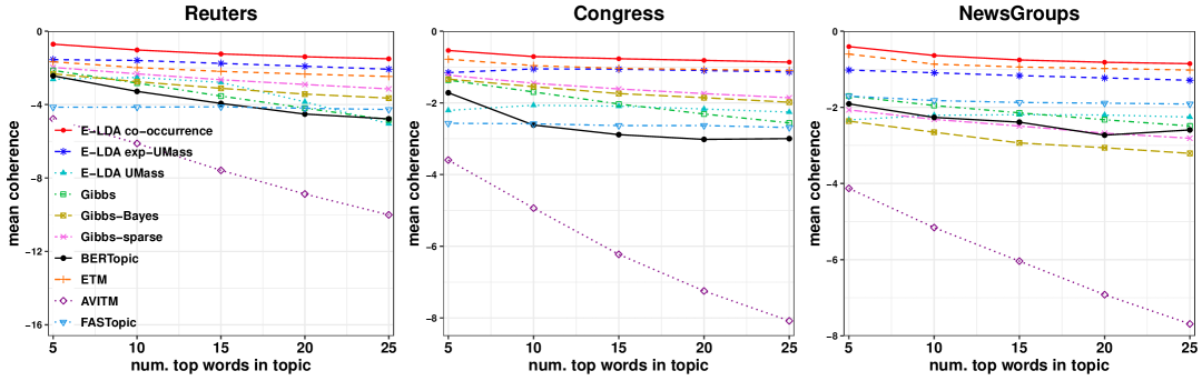
(a) Experiments Set 2: E-LDA topic coherence vs. baselines for various num. top words $h^{*}$ (10 run avg.).

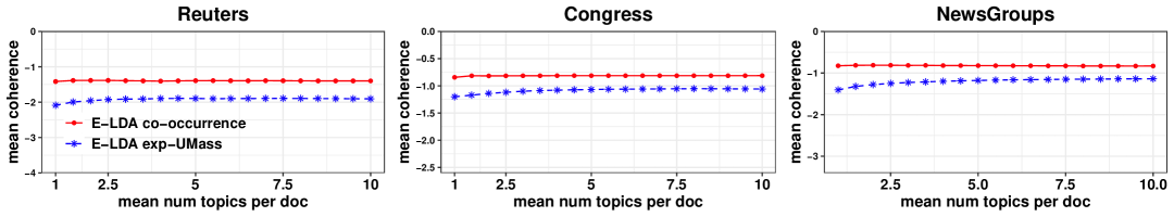
(b) Consistency of E-LDA’s coherence as solutions grow from sparse to dense, $1$$\rightarrow$$10$ topics-per-document.

Experiments Set 2 Results: Topics’ Semantic Quality. Fig. 2(a) compares the mean topic coherence of our solutions to baselines. E-LDA co-occurrence and exp-UMass solutions obtain $2.53$-$4.20$ and $1.18$-$1.67$ times better mean coherence, respectively, compared to the Gibbs topics when coherence scores computed based on the $5$ top words per topic (leftmost points in Fig. 2(a)). This suggests that E-LDA’s topics are significantly better than Gibbs topics at conveying a small and closely-related set of ‘keywords’ that are more semantically evocative of their topic’s subject matter. As we recompute coherence based on $h^{*}=10,\dots,25$ top words per topic (rightmost points in Fig. 2(a)), E-LDA co-occurrence and exp-UMass topics outperform Gibbs by a factor that increases to $2.92$-$3.21$ and $1.93$-$2.33$, respectively. This suggests that each E-LDA topic also captures more subtle semantic relationships beyond a handful of keywords, whereas Gibbs topics tend to exhibit more noise as we move down the list of their top words. Because coherence is a logarithmic measure, E-LDA’s several-fold improvement may be viewed as an exponential improvement in the degree to which E-LDA topics emphasize co-appearing words. Sparse and Bayesian variants of the Gibbs baselines improve slightly over the standard Gibbs on $2$ of the $3$ datasets, but neither obtains the semantic quality of co-occurrence and exp-UMass. Disaggregating the results, we note that (i) E-LDA co-occurrence’s plotted mean topic coherence outperforms the best single topic’s coherence of all Gibbs baselines’ topics; and (ii) E-LDA co-occurrence worst topic’s coherence outperforms the mean topic coherence of all Gibbs baselines. This holds regardless of $h^{*}$.

Considering neural and LLM-based baselines, E-LDA co-occurrence outperforms BERTopic, AVITM, and FASTopic by factors of $3.04$-$4.70$, $5.96$-$10.17$, and $2.24$-$5.84$, respectively. It also outperforms ETM by factors of $1.19$-$2.36$, despite the fact that ETM was designed as a coherence-improving algorithm. E-LDA exp-UMass outperforms BERTopic, AVITM, and FASTopic by factors of $1.46$-$2.72$, $3.08$-$7.09$, $1.48$-$2.67$ resp., and compares well to ETM (better on Reuters, slightly worse on NewsGroups).

Fig. 2(a) also plots the coherence of E-LDA initialized with an unmodified UMass topic generator. This basic approach performs relatively poorly (see App. Q), suggesting that E-LDA’s high coherence obtained via co-occurrence and exp-UMass topics are indicative of high semantic quality and not simply due to their generating function’s similarity to the function used to compute post hoc coherence. We note that the candidate sets of all three of our topic generators have identical mean coherence (coherence only depends on ranking, which is invariant to the exponential). The mean coherence of the candidate sets is -$2.9$, -$1.9$, -$1.8$ for Reuters, Congress, and NewsGroups. Observe that these mean coherences are significantly worse than the mean coherence of co-occurrence and exp-UMass solutions topics in Fig. 2(a). This is because our algorithms tend to select high-coherence topics from the candidate set under these (sparser) topic generators.

Consistency of E-LDA’s semantic quality advantage across sparse and dense solutions. Fig. 2(b) plots the consistency of E-LDA’s topic coherences as we grow its solutions from a maximally sparse arrangement of $1$ topic-per-document (equivalent to a document clustering) to a relatively dense $10$ topics-per-document. Here, we observe that E-LDA’s solutions exhibit remarkable consistency in terms of their high coherence regardless of the sparsity of the desired solution size. In short, E-LDA returns solutions of consistently high semantic quality regardless of whether researchers set them to produce a simple and sparse summary of their text data or a nuanced and dense one.

10 Conclusion

In this paper, we showed a novel combinatorial approach to topic modeling that efficiently and near-optimally solves LDA topic-word assignments under explicit sparsity constraints. We also showed that our approach permits practitioners to restrict the learned topics to those that meet standard interpretability criteria. Importantly, these guarantees and interpretability properties also apply when topics are used for causal inference. Finally, we showed that this approach learns topics of high semantic quality.

We have focused on LDA and sparsity constraints because these are the most practical tools for social science research. However, we emphasize that our techniques generalize to many topic model variations. They can also be solved under more sophisticated constraints such as packing or matroid constraints that permit significant flexibility compared to standard algorithms in terms of encoding domain-specific information into text models.

Impact statement

Mainstream social science applications for topic models models include text modeling for ethically fraught areas. For decisionmaking in such areas, it is ethically desirable and, increasingly, legally mandated to adopt models with strong guarantees and/or interpretability properties (Madiega, 2021). While neural and LLM/BERT-based topic models have recently shown impressive fidelity for text modeling in general, they lack such properties. We see our work as addressing this important gap.

Appendix A The LDA Model & Integrating out $\theta_{d}$

The LDA model states that the data is a corpus (set) $D$ of documents, where each document $d\in D$ is a multiset of words: $d=[w_{1},\dots,w_{|d|}]$. Suppose there are $k$ topics, where each topic is a distribution over all words in the vocabulary. LDA states that the text corpus is generated as follows: For each document $d$, we sample a document length $|d|$ and a document mixture distribution $\theta_{d}\sim Dirichlet(\alpha)$ over the $k$ topics. Then, to draw each of the $|d|$ words in $d$, we sample a topic $z_{d,i}\in\{1,\dots,k\}$, where $z_{d,i}\sim Categorical(\theta_{d})$, and from this topic we sample a word $w_{d,i}\sim Categorical(\phi_{z_{d,i}})$, where $\phi_{z}$ is the distribution over all words corresponding to topic $z$:

LDA generative model

0: Corpus $D$ of empty documents (multisets) $d_{1},\dots,d_{|D|}$, topics $\phi_{1}\dots\phi_{k}$, parameters $\alpha,\lambda$

 for document $d\in D$

     draw document length $|d|\sim\text{Poisson}(\lambda)$

     draw document distribution over topics $\theta_{d}\sim\text{Dirichlet}(\alpha)$

     for document-word index $i=1,\dots,|d|$

         draw topic $z_{d,i}\sim\text{Categorical}(\theta_{d})$

         draw word $w_{d,i}\sim\text{Categorical}(\phi_{z_{d,i}})$

         $d[i]\leftarrow w_{d,i}$

 return $D$

Now, denote by $Z$ all latent topics $z_{d,i}$ corresponding to each word in $D$; by $\Theta$ all documents’ topic mixtures $\{\theta_{1},\dots,\theta_{|D|}\}$; and by $\Phi$ the set of all topics $\{\phi_{1},\dots,\phi_{k}\}$. The joint model probability is:

$$\text{P}(D,Z,\Theta,\Phi\ |\alpha,\beta,\lambda)=\prod_{d\in D}\prod^{|d|}_{i=1}Cat(z_{d,i}|\theta_{d})\times c_{1}\prod_{d\in D}Dir(\theta_{d}|\alpha)$$ (5)

$$\ \ \ \ \ \ \ \ \ \ \ \ \ \ \ \ \ \ \ \ \ \ \ \ \ \ \ \ \ \ \ \ \ \ \ \ \ \ \ \ \times\prod_{d\in D}\prod^{|d|}_{i=1}Cat(w_{d,i}|z_{d,i},\ \phi_{z_{d,i}})\times c_{2}\prod^{k}_{\tau=1}Dir(\phi_{k}|\beta_{\tau})\times\prod_{d\in D}Poi(|d|\ |\ \lambda)$$

The second $Dir$ term is the $Dirichlet(\beta)$ prior on topics, and $c_{1}$ and $c_{2}$ are normalizing constants.

Documents’ topic mixtures $\theta_{d}$ can be integrated out of LDA’s joint probability as follows. We seek:

$$\text{P}(Z,\Phi\ |D,\alpha,\beta)\propto\int\underbrace{\prod_{d\in D}\prod^{|d|}_{i=1}Cat(z_{d,i}|\theta_{d})\times c_{1}\prod_{d\in D}Dir(\theta_{d}|\alpha)}\ d\theta_{d}$$

$$\ \ \ \ \ \ \ \ \ \ \ \ \ \ \ \ \ \ \ \ \ \ \ \ \ \ \ \ \ \ \ \ \ \ \ \ \ \ \ \ \times\prod_{d\in D}\prod^{|d|}_{i=1}Cat(w_{d,i}|z_{d,i},\ \phi_{z_{d,i}})\times c_{2}\prod^{k}_{\tau=1}Dir(\phi_{k}|\beta_{\tau})\times\prod_{d\in D}Poi(|d|\ |\ \lambda)$$

Documents are conditionally independent from each other. Denote the last three terms by $\Omega$:

$$=\prod_{d\in D}\int\prod^{|d|}_{i=1}Cat(z_{d,i}|\theta_{d})\times c_{1}\prod_{d\in D}Dir(\theta_{d}|\alpha)\ d\theta_{d}\times\Omega$$

Now, denote by $\theta_{d},\tau$ and $\alpha_{\tau}$ the $\tau$’th elements of $\theta_{d}$ and $\alpha$, respectively. Substituting the standard Dirichlet prior, we have:

$$=\prod_{d\in D}\int\frac{\Gamma(\sum^{k}_{\tau=1}\alpha_{\tau})}{\prod^{k}_{\tau=1}\Gamma(\alpha_{\tau})}\prod^{k}_{\tau=1}\theta_{d,\tau}^{a_{\tau}-1}\prod^{|d|}_{i=1}\theta_{d,z_{d}}\ d\theta_{d}\times\Omega$$

Changing variables in the product over each documents’ words, and letting $n_{d,\tau}$ denote the count of words in document $d$ that are assigned to topic $\tau$, so $\forall d,t,$ we have $0\leq n_{d,\tau}\leq|d|;\ \ \forall|d|,\sum^{k}_{\tau=1}n_{d,\tau}=|d|$. We have:

$$=\prod_{d\in D}\int\frac{\Gamma(\sum^{k}_{\tau=1}\alpha_{\tau})}{\prod^{k}_{\tau=1}\Gamma(\alpha_{\tau})}\prod^{k}_{\tau=1}\theta_{d,\tau}^{a_{\tau}-1}\prod^{k}_{\tau=1}\theta^{n_{d,\tau}}_{d,\tau}\ d\theta_{d}\times\Omega$$

$$=\prod_{d\in D}\int\frac{\Gamma(\sum^{k}_{\tau=1}\alpha_{\tau})}{\prod^{k}_{\tau=1}\Gamma(\alpha_{\tau})}\prod^{k}_{\tau=1}\theta_{d,\tau}^{a_{\tau}+n_{d,\tau}-1}\ d\theta_{d}\times\Omega$$

Multiplying by a fraction that is equal to $1$:

$$=\prod_{d\in D}\frac{\Gamma(\sum^{k}_{\tau=1}\alpha_{\tau})}{\prod^{k}_{\tau=1}\Gamma(\alpha_{\tau})}\frac{\prod^{k}_{\tau=1}\Gamma(n_{d,\tau}+\alpha_{\tau})}{\Gamma(\sum^{k}_{\tau=1}n_{d,\tau}+\alpha_{\tau})}\int\frac{\Gamma(\sum^{k}_{\tau=1}n_{d,\tau}+\alpha_{\tau})}{\prod^{k}_{\tau=1}\Gamma(n_{d,\tau}+\alpha_{\tau})}\prod^{k}_{\tau=1}\theta_{d,\tau}^{a_{\tau}+n_{d,\tau}-1}\ d\theta_{d}\times\Omega$$

Observe that the integral is now over the entire domain of a Dirichlet PDF, so it evaluates to $1$:

$$=\prod_{d\in D}\frac{\Gamma(\sum^{k}_{\tau=1}\alpha_{\tau})}{\prod^{k}_{\tau=1}\Gamma(\alpha_{\tau})}\frac{\prod^{k}_{\tau=1}\Gamma(n_{d,\tau}+\alpha_{\tau})}{\Gamma(\sum^{k}_{\tau=1}n_{d,\tau}+\alpha_{\tau})}$$

$$\ \ \ \ \ \ \ \ \ \ \ \ \ \ \ \ \ \ \ \ \ \ \ \ \times\prod_{d\in D}\prod^{|d|}_{i=1}Cat(w_{d,i}|z_{d,i},\ \phi_{z_{d,i}})\times c_{2}\prod^{k}_{\tau=1}Dir(\phi_{k}|\beta_{\tau})\times\prod_{d\in D}Poi(|d|\ |\ \lambda)$$ (6)

Ignoring the nuisance document length term (which is standard [Blei et al., 2003]), then for a fixed set of topics $\Phi$ we arrive at the canonical MAP topic assignment inference problem studied in seminal work by Sontag and Roy [2011]. Taking logarithms of the following gives the expression in Section 2:

$$\text{P}(Z|D)\propto\displaystyle\prod_{d\in D}\Big{(}\frac{\Gamma(\sum^{k}_{\tau=1}\alpha_{\tau})\prod^{k}_{\tau=1}\Gamma(n_{d,\tau}+\alpha_{\tau})}{\Gamma(\sum^{k}_{\tau=1}\alpha_{\tau}+|d|)\prod^{k}_{\tau=1}\Gamma(\alpha_{\tau})}\prod^{|d|}_{i=1}Cat(w_{d,i}|z_{d,i},\ \phi_{z_{d,i}})\Big{)}$$ (7)

Appendix B Deferred proof of Theorem 1

Theorem.

$$\displaystyle\lim_{\alpha\rightarrow\infty}\big{(}\underset{Z}{\mathrm{argmax}}\ \log\text{P}(Z|D)\big{)}=\underset{Z}{\mathrm{argmax}}\sum_{d\in D}\sum^{|d|}_{i=1}\log Cat(w_{i,d}|z_{i,d},\ \phi_{z_{i,d}})$$ (8)

Proof. From Section 1 we have:

$$\log\text{P}(Z|D)\propto\sum_{d\in D}\Big{(} \underbrace{\sum^{|d|}_{i=1}\log Cat(w_{d,i}|z_{d,i},\phi_{z_{d,i}})}_{likelihood}+\underbrace{\sum^{k}_{\tau=1}\log\Gamma(n_{d,\tau}+\alpha_{\tau})}_{sparsity}$$

$$\enspace+\underbrace{\log\Gamma(\sum^{k}_{\tau=1}\alpha_{\tau})-\log\Gamma(\sum^{k}_{\tau=1}\alpha_{\tau}+|d|)-\sum^{k}_{\tau=1}\log\Gamma(\alpha_{\tau})}_{constant}\Big{)}$$ (9)

We will use the following well-known asymptotic property of $\Gamma$ functions: for $r\in\mathbb{C}$, $lim_{r\rightarrow\infty}\Gamma(q+r)=\Gamma(q)q^{r}$. After taking logs and rearranging, we have the property $lim_{r\rightarrow\infty}\left[\log\frac{\Gamma(kq+r)}{\log(\Gamma(kq))}-r\log(kq)\right]=0$ for $k>0$.

Consider the limit for a single document, and let $\mathcal{L}$ denote the likelihood term that is independent of $\alpha$. Rearranging, we have:

$$\lim_{\alpha\rightarrow\infty}\Big{[}-\log\frac{\Gamma(\sum_{\tau=1}^{k}\alpha_{i}+|d|)}{\Gamma(\sum_{\tau=1}^{k}\alpha_{i})}+\sum^{k}_{\tau=1}\log\frac{\Gamma(\alpha_{i}+n_{d,\tau})}{\Gamma(\alpha_{i})}+\mathcal{L}\Big{]}$$

$$= \lim_{\alpha\rightarrow\infty}\Big{[}-\log\frac{\Gamma(k\alpha+|d|)}{\Gamma(k\alpha)}+\sum^{k}_{\tau=1}\log\frac{\Gamma(\alpha+n_{d,\tau})}{\Gamma(\alpha)}+0-\sum^{k}_{\tau=1}0\Big{]}+\mathcal{L}$$

Applying our asymptotic property with $$q=k\alpha,\ r=|d| k>0$$ and noting we have:

$$= \lim_{\alpha\rightarrow\infty}\Big{[}-\log\frac{\Gamma(k\alpha+|d|)}{\Gamma(k\alpha)}+\sum^{k}_{\tau=1}\log\frac{\Gamma(\alpha+n_{d,\tau})}{\Gamma(\alpha)}$$

$$\ \ \ \ \ \ \ \ \ \ \ \ \ \ \ \ \ \ \ \ \ +\Big{(}\log\frac{\Gamma(k\alpha+|d|)}{\Gamma(k\alpha)}-|d|\log(k\alpha)\Big{)}-\sum^{k}_{\tau=1}0\Big{]}+\mathcal{L}$$

$$= \lim_{\alpha\rightarrow\infty}\Big{[}\sum^{k}_{\tau=1}\log\frac{\Gamma(\alpha+n_{d,\tau})}{\Gamma(\alpha)}-|d|\log(k\alpha)-\sum^{k}_{\tau=1}0\Big{]}+\mathcal{L}$$

Applying our asymptotic property $$k q=\alpha,\ r=n_{d,\tau} \tau=1\dots k$$ times with for we have:

$$= \lim_{\alpha\rightarrow\infty}\Big{[}\sum^{k}_{\tau=1}\log\frac{\Gamma(\alpha+n_{d,\tau})}{\Gamma(\alpha)}-|d|\log(k\alpha)-\Big{(}\sum_{\tau=1}^{k}\Big{(}\log\frac{\Gamma(\alpha+n_{d,\tau})}{\Gamma(\alpha)}-n_{d,\tau}\log\alpha\Big{)}\Big{)}\Big{]}+\mathcal{L}$$

$$= \lim_{\alpha\rightarrow\infty}\Big{[}-|d|\log(k\alpha)+\sum_{\tau=1}^{k}n_{d,\tau}\log\alpha\Big{]}+\mathcal{L}$$

$$= \lim_{\alpha\rightarrow\infty}\Big{[}-|d|\log(k\alpha)+|d|\log\alpha\Big{]}+\mathcal{L}$$

$$= \lim_{\alpha\rightarrow\infty}\Big{[}-|d|\log k\Big{]}+\mathcal{L}$$

$$= -|d|\log k+\mathcal{L}$$

After substituting for $$\mathcal{L}$$ and adding up this single-document limit over all documents we have:

$$\displaystyle\lim_{\alpha\rightarrow\infty}\big{(}\underset{Z}{\mathrm{argmax}}\ \log\text{P}(Z|D)\big{)}=\underset{Z}{\mathrm{argmax}}\Big{[}-\log(k)\cdot\displaystyle\sum_{d\in D}|d|+\displaystyle\sum_{d\in D}\displaystyle\sum^{|d|}_{i=1}\log Cat(w_{i,d}|z_{i,d},\ \phi_{z_{i,d}})\Big{]}$$

$$=\underset{Z}{\mathrm{argmax}}\displaystyle\sum_{d\in D}\displaystyle\sum^{|d|}_{i=1}\log Cat(w_{i,d}|z_{i,d},\ \phi_{z_{i,d}})\text{ \ \ as the left term above is const. independent of $\alpha$.}$$

Appendix C Deferred proof of submodularity

Recall that original objective function $f$ from eq. 3 is:

$$\text{\emph{Objective function:} }f(E) =\max\big{[}\log P(Z|D,E)\big{]}$$ (10)

$$=\sum_{d\in D}\sum_{i=1}^{|d|}\ \max_{\tau\in E_{d}}(\log\phi_{\tau}[w_{d,i}])$$

$$\text{find }\underset{{\{\tau\Rightarrow d\},\tau\in\Phi,d\in D}}{\operatorname{argmax}}f(E) \text{\ s.t.}\ |E|\leq\kappa|D|;\ |E_{d}|\geq 1,\forall d$$

We noted that one challenge is that $f$ is undefined when some document has no links in $E$. We addressed this by extending the initialization technique of Gomes and Krause [2010] by linking each document to a single improper placeholder topic $p$ with infinitesimal probability on each word, then maximizing $\dot{f}$ (equivalent to maximizing $f$): $\dot{f}(E)=f(E\cup P)-f(P)$, where $P$ is the set of placeholder topics.

We now show that objective $\dot{f}(E)$ is a monotone submodular function. First, observe that the objective $\dot{f}$ is monotone, as adding more links to $E$ cannot decrease $\dot{f}(E)$ due to the $\max$ function. Now, consider the marginal value $\dot{f}_{E}(A)\coloneqq\dot{f}(E\cup A)-\dot{f}(E)$ of adding links $A=\{[\tau\Rightarrow d]\}$ to $E$.

$$\dot{f}_{E}(A)\coloneqq \dot{f}(E\cup A)-\dot{f}(E)\ \ \text{\ \ \ \ \ is our marginal value function}.$$

$$= f(E\cup A\cup P)-f(P)-\big{(}f(E\cup P)-f(P)\big{)}$$

$$= \sum_{d\in D}\sum_{i=1}^{|d|}\ \max_{\tau^{{}^{\prime}}\in(E_{d}\cup A\cup P)}(\log\phi_{\tau^{{}^{\prime}}}[w_{d,i}])-\sum_{d\in D}\sum_{i=1}^{|d|}\ \max_{\tau^{{}^{\prime\prime}}\in P}(\log\phi_{\tau^{{}^{\prime\prime}}}[w_{d,i}])$$

$$\ \ \ \ \ \ \ -\Big{(}\sum_{d\in D}\sum_{i=1}^{|d|}\ \max_{\tau\in(E_{d}\cup P)}(\log\phi_{\tau}[w_{d,i}])-\sum_{d\in D}\sum_{i=1}^{|d|}\ \max_{\tau^{{}^{\prime\prime}}\in P}(\log\phi_{\tau^{{}^{\prime\prime}}}[w_{d,i}])\Big{)}$$

$$= \sum_{d\in D}\sum_{i=1}^{|d|}\ \max_{\tau^{{}^{\prime}}\in(E_{d}\cup A\cup P)}(\log\phi_{\tau^{{}^{\prime}}}[w_{d,i}])-\sum_{d\in D}\sum_{i=1}^{|d|}\ \max_{\tau\in(E_{d}\cup P)}(\log\phi_{\tau}[w_{d,i}])$$ (11)

For a single document $$d$$, we have:

$$= \sum_{i=1}^{|d|}\ \max_{\tau^{{}^{\prime}}\in(E_{d}\cup A\cup P)}(\log\phi_{\tau^{{}^{\prime}}}[w_{d,i}])-\sum_{i=1}^{|d|}\ \max_{\tau\in(E_{d}\cup P)}(\log\phi_{\tau}[w_{d,i}])$$

$$= \sum_{i=1}^{|d|}\Big{(}\ \max_{\tau^{{}^{\prime}}\in(E_{d}\cup A\cup P)}(\log\phi_{\tau^{{}^{\prime}}}[w_{d,i}])-\max_{\tau\in(E_{d}\cup P)}(\log\phi_{\tau}[w_{d,i}])\Big{)}$$

Denote by $$\mathbf{1}(\cdot) 1 0$$ a function that takes the value of if its argument is true and otherwise. Now:

$$= \sum_{i=1}^{|d|}\Big{(}\big{(}\ \max_{\tau^{{}^{\prime}}\in A}(\log\phi_{\tau^{{}^{\prime}}}[w_{d,i}])-\max_{\tau\in(E_{d}\cup P)}(\log\phi_{\tau}[w_{d,i}])\big{)}\cdot\mathbf{1}\big{(}\max_{\tau^{{}^{\prime}}\in A}(\phi_{\tau^{{}^{\prime}}}[w_{d,i}])>\max_{\tau\in(E_{d}\cup P)}(\phi_{\tau}[w_{d,i}])\big{)}\Big{)}$$ (12)

Observe that as the set $E_{d}$ grows (i.e. $E_{d}$ is expanded to include more topics linked to $d$), the first term, $\max_{\tau^{{}^{\prime}}\in A}(\log\phi_{\tau^{{}^{\prime}}}[w_{d,i}])$ is fixed and the second term, $\max_{\tau\in(E_{d}\cup P)}(\log\phi_{\tau}[w_{d,i}])$, is nondecreasing. Therefore, observe (1) the sum $\sum_{i=1}^{|d|}\big{(}\ \max_{\tau^{{}^{\prime}}\in A}(\log\phi_{\tau^{{}^{\prime}}}[w_{d,i}])-\max_{\tau\in(E_{d}\cup P)}(\log\phi_{\tau}[w_{d,i}])\big{)}$ is nonincreasing. Then observe (2) that any topic $\tau\in A$ will be the maximum-probability topic for (weakly) fewer words in $d$, thus it will contribute (weakly) fewer terms to $\dot{f}$ due to the $\mathbf{1}(\cdot)$ function. Putting these together, we have that the marginal value of adding $A$ to $E_{d}$ is weakly decreasing as $E_{d}$ grows: $\dot{f}_{E_{d}}(A)\geq\dot{f}_{E^{\prime}_{d}}(A),\ \ \forall E_{d}\subseteq E^{\prime}_{d},\ \tau\in A\subseteq\Phi,\text{ and }d\in D$.

Finally, this analysis supposed a corpus of a single document. However, per line 11, $\dot{f}$ is a sum of $|D|$ per-document submodular functions. Sums of submodular functions are also submodular.

Appendix D Unconstrained problem formulations & expected number of unique topics per document

Observe that in the unconstrained case (i.e. where each document can have unlimited topics up to one unique topic per word), then finding $d$’s MAP topic-word assignments, $\operatorname{argmax}_{Z_{d}}\text{P}(Z_{d}|d)$, is easy. In that case, we just assign each word in the data to the topic in $\Phi$ with the highest probability of drawing it: $z_{d,i}=\operatorname{argmax}_{\tau\in\Phi}\phi_{\tau}[w_{d,i}]$. Summing these, we have:

$$\max_{Z}\big{[}\log P(Z|D)\big{]}=\sum_{d\in D}\sum_{i=1}^{|d|}\ \max_{\tau\in\Phi}(\log\phi_{\tau}[w_{d,i}])$$ (13)

However, this unconstrained problem returns practically unusable, maximally overfit solutions where each word in a document may be associated with a different topic. In the analysis below, we show below that in the unconstrained problem, the expected number of unique topics-per-document is well-approximated by $|\Phi|(1-e^{-|d|/|\Phi|})$. For practical-sized datasets such as (for example) Twitter datasets commonly used in social science research, $|\Phi|$ exceeds the word count of any single document (Tweet). In that case, the unconstrained MAP solution assigns each document a number of unique topics that approaches one unique topic-per-word. In other words, the unconstrained MAP solution returns a ‘worst-case overfit’. Even when the number of topics is the same as the wordcount of a document (e.g. $100$), the unconstrained problem’s MAP solution assigns each $100$-word tweet $|\Phi|(1-e^{-|d|/|\Phi|})=100(1-e^{-100/100})\approx 63.2$ unique topics per $100$-word document in expectation. As such, the unconstrained problem formulation yields unusably dense solutions for practical problem instances.

Indeed, as we discussed in Section 2, one of the primary problems with using documents’ underlying distributions $\theta_{d}$ for downstream social science analysis is that for many practical datasets such as Twitter data, the number of topics required to adequately model the dataset exceeds the length of any document: $k>|d|$. As such, a document’s underlying topic distribution vector $\theta_{d}$ is not a dimensionality reduction (which is often the goal of using LDA in social science application domains), but a dimensionality expansion. Absent a sparsity constraint, the MAP topic-word assignments exhibit similarly undesirable dimensionality. These issues motivate our sparsity-constrained problem formulation.

More formally, we obtain the expected average number of topics per document in the MAP solution for a given unconstrained problem (i.e. where each document can have unlimited topics up to one unique topic per word) as follows. For a single document, in the infinite limit of $\alpha$ the probability of drawing zero words from topic $\tau$ is $\Big{(}\frac{(|\Phi|-1)}{|\Phi|}\Big{)}^{|d|}$. The probability of drawing at least one word from topic $\tau$ is the complement $1-\Big{(}\frac{(|\Phi|-1)}{|\Phi|}\Big{)}^{|d|}$. Therefore the expected number of unique topics in document $d$ is $|\Phi|\Big{[}1-\Big{(}\frac{(|\Phi|-1)}{|\Phi|}\Big{)}^{|d|}\Big{]}$. To understand how this scales, we can rearrange and use the standard limit approximation to obtain the useful approximation $|\Phi|\Big{[}1-\Big{(}\frac{(|\Phi|-1)}{|\Phi|}\Big{)}^{|d|}\Big{]}\approx|\Phi|(1-e^{-|d|/|\Phi|})$.

To obtain the expected average number of unique topics per document in the corpus, we just take the expectation over all documents, $\frac{1}{|D|}\sum_{d\in D}|\Phi|\Big{[}1-\Big{(}\frac{(|\Phi|-1)}{|\Phi|}\Big{)}^{|d|}\Big{]}=|\Phi|(1-1/|D|)\sum_{d\in D}(1-1/|\Phi|)^{|d|}$. Applying this to our approximation gives $|\Phi|(1-1/|D|)\sum_{d\in D}(1-1/|\Phi|)^{|d|}\approx\frac{\Phi}{|D|}\sum_{d\in D}(1-e^{-|d|/|\Phi|})$.

Unconstrained problem with known $\theta$. Alternatively one could also consider a variant of the unconstrained problem formulation where we assume that documents’ underlying topic distributions $\theta_{d}$ are also known. In that case, we could easily obtain the MAP topic-word assignments by maximizing:

$$\max_{Z}\big{[}\log P(Z|D)\big{]}=\sum_{d\in D}\sum_{i=1}^{|d|}\ \max_{\tau\in\Phi}(\log\theta_{d}[\tau]\cdot\phi_{\tau}[w_{d,i}])$$ (14)

However, the assumption that $\theta_{d}$ are known is very strong. Mainstream algorithms such as Gibbs provide no guarantees for $\theta_{d}$. It is possible to obtain estimates of $\theta_{d}$ via e.g. the algorithms of Arora et al. [2016b], but these algorithms yield $\theta_{d}$ with errors that are $o(1/|E_{d}|)$. In other words, for that approach, solutions that are more desirably sparse exhibit more errors in terms of $\theta_{d}$, yielding more errors in terms of the resulting MAP topic-word assignments. We contrast these problems with the near optimal deterministic guarantees of our approach.

Appendix E Simple Greedy Algorithm

Consider the simple Greedy algorithm that grows the solution set of topic-to-document links $E$ by iteratively adding the link with the greatest marginal contribution to $\dot{f}$. We formalize this algorithm and derive its complexity below. While it is practically infeasible, it has near-optimal global and per-document approximation guarantees. Our optimized FastGreedy-E-LDA algorithm accelerates this simple Greedy algorithm while maintaining the same guarantees.

Simple-Greedy-E-LDA

0: Corpus $D$, Candidate topic set $\Phi$, Sparsity constraint upper-bound $\kappa$, Phantom topic links $\mathcal{P}$

 initialize $E\leftarrow\mathcal{P}$

 for $\kappa|D|$ steps do

      $[\tau^{*}\Rightarrow d^{*}]\leftarrow$ the topic-doc link that adds the highest marginal value, $\underset{\tau\in\Phi,d\in D}{\operatorname{argmax}}\ f_{E}([\tau\Rightarrow d])$

      $E\leftarrow[\tau^{*}\Rightarrow d^{*}]$

 return    $E\backslash\mathcal{P}$

Where each phantom topic $\phi_{phantom}$ in the phantom topic links $\mathcal{P}$ is a topic with constant (improper) small probability on all words, e.g. $[1^{-10}]^{|V|}$.

1-1/e Approximation Guarantee.

For completeness, we show Simple-Greedy’s $1-1/e$ approximation guarantee via the classic result of Nemhauser and Wolsey [1978]. Let $E^{OPT}$ denote the optimal (maximum value) solution of size $\kappa|D|$, with value $\dot{f}(E^{OPT})=OPT$. Let $E^{i}$ denote Simple-Greedy’s solution at iteration $i$. We claim via induction that for its iterations $0\leq i\leq\kappa|D|$:

$$\dot{f}(E^{OPT})-\dot{f}(E^{i})\leq\Big{(}1-\frac{1}{\kappa|D|}\Big{)}^{i}\dot{f}(E^{OPT})$$ (15)

This is trivially true for $i=0$. First, consider Simple-Greedy’s solution $E^{i-1}$ at a previous iteration $i-1$. Because there are $|O\backslash E^{i-1}|\leq\kappa|D|$ more elements in $E^{OPT}$ than in $E^{i-1}$, and the ‘best’ one we can add to $E^{i-1}$ now is what Simple-Greedy will add first, then we have (by subadditivity):

$$\dot{f}(E^{OPT})-\dot{f}(E^{i-1})\leq\sum_{a\in E^{OPT}\backslash E^{i-1}}\dot{f}_{E^{i-1}}(a)$$

$$\frac{1}{\kappa|D|}\big{(}\dot{f}(E^{OPT})-\dot{f}(E^{i-1})\big{)}\leq\dot{f}_{E^{i-1}}(a_{i})$$ (16)

Now, returning to our hypothesis, we can expand left-hand-side (i.e. ‘separate out’ the last link that was added to Simple-Greedy’s solution at iteration $i$):

$$\dot{f}(E^{OPT})-\dot{f}(E^{i}) =\dot{f}(E^{OPT})-\dot{f}(E^{i-1})-\dot{f}_{E^{i-1}}(a_{i})$$

$$\leq\dot{f}(E^{OPT})-\dot{f}(E^{i-1})-\frac{1}{\kappa|D|}\big{(}\dot{f}(E^{OPT})-\dot{f}(E^{i-1})\big{)}\text{ \ substituting eq. \ref{useful}}$$

$$=\big{(}1-\frac{1}{\kappa|D|}\big{)}\big{(}\dot{f}(E^{OPT})-\dot{f}(E^{i-1})\big{)}$$

$$\leq\big{(}1-\frac{1}{\kappa|D|}\big{)}^{i}\dot{f}(E^{OPT})$$

Now set $i=\kappa|D|$, rearrange, and use $(1-\frac{1}{\kappa|D|})^{\kappa|D|}\leq 1/e$ to obtain $\dot{f}(E)\geq(1-1/e)OPT$.

Appendix F Complexity of Simple-Greedy

We now derive the complexity of the vanilla Simple-Greedy algorithm described in Section 4 and compare it to the Accelerated-Greedy-E-LDA algorithm described here:

Simple-Greedy completes in $\kappa|D|$ iterations. Each iteration $i$ of Simple-Greedy computes the marginal value of $|\Phi||D|-i$ links. Without the speedups described in FastGreedy-E-LDA, computing one of these marginal values entails solving $f(E^{i}\cup[\tau\Rightarrow d])-f(E^{i})$, where $[\tau\Rightarrow d]$ is a new topic-doc link (where $E^{i}$ denotes the solution at iteration $i$). Computing a value of $f$ requires, for each document in $D$, finding the max log probability of each word in $d$ among $E_{d}$ topics (or $E_{d}+1$ topics for $f(E^{i}\cup[\tau\Rightarrow d])$), then summing the result. Denote the number of words in the longest document by $\ell$. Thus each marginal value requires $O(\ell|E_{d}||D|)$ which is $O(\ell\kappa|D|)$. An iteration of Simple-Greedy requires computing $O(|\Phi||D|)$ such marginal values, so each iteration is $O(\ell\kappa|\Phi||D|^{2})$.

Appendix G FastGreedy-E-LDA details and analysis

We now describe the main ideas we use to obtain FastGreedy-E-LDA’s fast theoretic and practical runtimes while maintaining the deterministic near-optimal guarantees of the vanilla SimpleGreedy algorithm. We analyze complexity below.

• Improving the per-iteration complexity by the first $|D|$-factor. Simple-Greedy evaluates the marginal value of all $|D||\Phi|$ links each iteration. These costly operations can be avoided through thoughtful design. Specifically, after a link $[\tau^{*}\Rightarrow d^{*}]$ is added to the solution set $E$, the topic-word assignments for document $d^{*}$ may be updated, but these are independent of all other documents’ assignments in LDA. Therefore, the marginal value of all links that do not include $d^{*}$ are unchanged in the next iteration. These may be memoized [Iyer and Bilmes, 2019] rather than recomputed, so each iteration we only need to recompute marginal values of at most $|\Phi|$ remaining links to $d^{*}$. Then, rather than check the maximum marginal valued link out of the $|\Phi||D|$ links to add to our solution each iteration, we save and update the best link for each document in a max-heap. Thus, we extract the best element in $O(\log|D|)$ instead of $O(|\Phi||D|)$.

• Improving the per-iteration complexity by another $2|D|$-factor. In a vanilla implementation, computing a single marginal value of a new link $[\tau\Rightarrow d]$ requires summing over the log-probabilities of all $|D|$ documents. However, due to the conditional independence of documents in LDA, only the log probability of $d^{*}$ changes each iteration. After cancelling these terms from the difference $f_{E}([\tau\Rightarrow d])=f(E\cup[\tau\Rightarrow d])-f(E)$, we can compute the marginal value of $f_{E}([\tau\Rightarrow d])$ by summing only over the words in $d$, which accelerates computation by a factor of $2|D|$ each iteration.

• Improving the per-iteration complexity by another $\kappa$-factor. We can also memoize the log probabilities associated with the current topic-word assignments $z_{i,d}$. Then, when we compute a marginal value, we need not find the max log probability for each word among the $E_{d}$ topics connected to $d$, which saves an additional $\kappa$ factor per iteration.

• Fast start. Because documents in LDA are conditionally independent and each document must be drawn from at least one topic, we can efficiently initialize the set $E$ by adding a link between each document and the highest marginal value topic for that document. This yields the first $|D|$ links after computing a single round of marginal values (equivalent to one step of the for-loop instead of $|D|$ rounds). Moreover, this first round of marginal values can be efficiently computed as the product of the document-word matrix and $\Phi^{T}$ minus the phantom topic values (see the FastInitialize subroutine).

• Lazy updates. Our approach can also leverage lazy updates. Lazy updates offer no provable improvement in the worst-case, but often result in dramatic practical speedups [Minoux, 1978, Mirzasoleiman et al., 2015]. In particular, it is practically advantageous to lazily update the marginal values $M[d^{*},:]$, as we do not need to know all marginal values, but just the best one, which in the best case removes an $O(|\Phi|)$ factor of computation each iteration. Also, when recomputing the marginal value of a link over various iterations, if the link does not improve the log probability of a word in an iteration then it will not improve the log probability of that word in any subsequent iteration, so we can skip the word in the marginal value summation.

• Fast indexing via the heap. In a practical fast implementation, each row of $\mathbf{P}$ and $\mathbf{M}$ can be stored in the heap $\mathbb{m}$ attached (e.g. in a tuple) to their corresponding elements to avoid the cost of indexing into $|D|$-sized storage.

Complexity of FastGreedy-E-LDA.

To simplify analysis, we will regard the addition of each of the $|D|$ initial links added by FastInitialize as ‘iterations’ of FastGreedy-E-LDA, despite the fact that these initial ‘iterations’ are slightly faster. FastGreedy-E-LDA completes in $\kappa|D|$ iterations. Each iteration extracts the maximum-marginal-valued link $[t^{*}\Rightarrow d^{*}]$ from the max-heap $\mathbb{m}$, which is $O(\log|D|)$. The next line updates the current log probabilities corresponding to $d^{*}$’s current topic-word assignments $z_{d,1},\dots,z_{d,|d|}$, which is bounded by the wordcount of the longest document, $O(\ell)$. The total log probability of document $d$ is then updated in constant time (via memoization). Then the marginal values for all remaining links to $d^{*}$ are updated, and we also check which of these links has the greatest marginal value, which has complexity $O(\ell|\Phi|)$. Finally, we insert this link with the greatest marginal value for $d^{*}$ into the max-heap $\mathbb{m}$, which is $O(\log|D|)$. We have a total per-iteration complexity of just $O(\log|D|+\ell|\Phi|)$.

Appendix H Comparison with Lazier-Than-Lazier-Greedy

We now show that FastGreedy-E-LDA has better complexity than the fastest generic serial algorithm for submodular optimization, Lazier-than-lazy-greedy (LTLG) [Mirzasoleiman et al., 2015], despite the fact that FastGreedy-E-LDA obtains deterministically near-optimal solutions whereas LTLG’s guarantees hold only in expectation.

Lazier-Than-Lazy-Greedy (LTLG)

0: Corpus $D$, Candidate topic set $\Phi$, Sparsity constraint upper-bound $\kappa$, Phantom topic links $\mathcal{P}$

 initialize $E\leftarrow\mathcal{P}$

 for $i\in\{1,\dots,\kappa|D|\}$ steps do

     $R\leftarrow$ a random subset of remaining topic-document links $[\tau\Rightarrow d]$ not in $E$, $\tau\in\Phi,d\in\mathcal{D}$

      $[\tau^{*}\Rightarrow d^{*}]\leftarrow$ the topic-doc link in $R$ with the highest marginal value, $\underset{\tau\in\Phi,d\in D}{\operatorname{argmax}}\ f_{E}([\tau\Rightarrow d])$

      $E\leftarrow[\tau^{*}\Rightarrow d^{*}]$

 return    $E\backslash\mathcal{P}$

Complexity of Lazier-Than-Lazy-Greedy [Mirzasoleiman et al., 2015].

LTLG is the fastest generic probabilistic serial algorithm for maximizing a submodular function [Mirzasoleiman et al., 2015]. It obtains a $(1-1/e-\epsilon)$ approximation guarantee in expectation, where $\epsilon$ is user-chosen. To accomplish this, LTLG proceeds identically to Simple-Greedy, except that at each of its $\kappa|D|$ iterations rather than evaluating the marginal value of all remaining links, it evaluates a random set of only $\frac{|\Phi||D|}{\kappa|D|}log(1/\epsilon)=\frac{|\Phi|}{\kappa}log(1/\epsilon)$ links sampled uniformly at random from the remaining links not yet added to the solution. It then adds the highest marginal value link in this random sample to the solution.

When applied to our objective $\dot{f}$, LTLG can also be accelerated via our memoization techniques ($\mathbf{P}$ and $\mathbf{p}$ in FastGreedy-E-LDA), which alleviate the need to sum over all $|D|$ documents’ log probabilities and maximize over all already-linked topics for each marginal value. After applying these speedups, each marginal value can be computed at a cost of $O(\ell)$. Finding the best sample of all marginal values for an iteration is O($\frac{|\Phi|}{\kappa}log(1/\epsilon)$) (i.e. the sample complexity per iteration).

The result is a per-iteration complexity of $O((\ell|\Phi|/\kappa)\log(1/\epsilon))$ for each of the $\kappa|D|$ iterations. However, this ignores the additional complexity of drawing $\frac{|\Phi|}{\kappa}\log(1/\epsilon)$ random samples each iteration, as well as the complexity of indexing into the memoized values each iteration. In practice, these random generation and indexing costs are significant, as the ground set is large. Also, unlike in the FastGreedy-E-LDA algorithm, the elements accessed each iteration by LTLG are non-proximal in memory (and associated with many different documents) due to the uniform random sampling, so there is no obvious way to apply the heap technique to improve indexing costs.

Appendix I Deferred description of the FAST parallel algorithm

We reprint the FAST-FULL outer-loop and FAST algorithms from Breuer et al. [2020] below using our E-LDA notation for completeness. As in that paper, the purpose of the outer loop algorithm is to generate various guesses $v\in V$ of the optimal constrained E-LDA objective value, which is denoted by $\texttt{OPT}\coloneqq\max\dot{f}(E)$ s.t. $|E|\leq\kappa|D|$. These guesses of OPT are then used to instantiate the inner FAST algorithm. This inner FAST algorithm then binary searches over these guesses for the largest guess $v$ that obtains a solution $E$ that is a $1-1/e$ approximation to $v$, resulting in an overall E-LDA solution that is near optimal.

Algorithm 1 Fast-Full: the full algorithm

0: function $f$, cardinality constraint $\kappa$, accuracy parameter $\varepsilon$

 $S\leftarrow$ the highest value $\kappa|D|$ links $[\tau\Rightarrow d]$

 $V\leftarrow\textsc{Geom}(f([\tau^{*}\Rightarrow d^{*}]),\max_{|S|\leq\kappa|D|}\sum_{[\tau\Rightarrow d]\in S}f([\tau\Rightarrow d]),1-\varepsilon)$

 $v^{\star}\leftarrow$ B-Search$(\max\{v\in V:f(E_{v})\geq(1-1/e)v\})$

      where $E_{v}\leftarrow\textsc{Fast}(v)$

 return $E_{v^{\star}}$

The main routine Fast   generates at every iteration a uniformly random sequence $a_{1},\ldots,a_{|X|}$ of the remaining set $X$ of topic-document links that have not yet been discarded. After the preprocessing step which adds to the current solution $E$ some topic-document links guaranteed to have high marginal contribution, the algorithm identifies the maximum sequence prefix length $i^{*}$ (i.e. the first $i^{*}$ links of the sequence) such that there is a large fraction of not-yet-added links in $X$ with high contribution to $E\cup A_{i^{\star}-1}$, and adds this sequence prefix of topic-document links to the current solution $E$.

Algorithm 2 Fast: the Fast Adaptive Sequencing Technique algorithm

0: $f$, constraint $\kappa|D|$, guess $v$ for OPT, accuracy parameter $\varepsilon$, sample complexity $m$

 $E\leftarrow\emptyset$

 while $|E|<\kappa|D|$ and number of iterations $<\varepsilon^{-1}$ do

       $X\leftarrow(\{[\tau\Rightarrow d]\},\tau\in 1\dots|\Phi|,d\in D),\hat{t}\leftarrow(1-\varepsilon)(v-f(E))/(\kappa|D|)$

       while $X\neq\emptyset$ and $|E|<\kappa|D|$ do

            (Denote single links $[t\Rightarrow d]$ by $\ a\$ to simplify notation)

             $a_{1},\ldots,a_{|X|}\leftarrow\textsc{Sequence}(X,|X|)$

             $A_{i}\leftarrow a_{1},\ldots,a_{i}$

             $E\leftarrow E\cup\{a_{i}:f_{E\cup A_{i-1}}(a_{i})\geq\hat{t}\}$

            $X_{0}\leftarrow\{a\in X:f_{E}(a)\geq\hat{t}\}$

             if $|X_{0}|\leq(1-\varepsilon)|X|$ then

                   $X\leftarrow X_{0}$ and continue to next iteration

             $R\leftarrow\textsc{Sample}(X,{m})$,

            $I\leftarrow\textsc{Geom}(1,\kappa|D|-|E|,1-\varepsilon)$

            $R_{i}\leftarrow\left\{a\in R:f_{E\cup A_{i-1}}(a)\geq\hat{t}\right\},$ for $i\in I$

             $i^{\star}\leftarrow$ B-Search$(\max\{i:|R_{i}|\geq(1-2\varepsilon)|R|\})$

             $E\leftarrow E\cup A_{i^{\star}}$

 return $E$

Appendix J Deferred analysis of simulating Fast

As described in Theorem 3 [Breuer et al., 2020] and above, the parallel Fast algorithm obtains near-optimal solutions w.p. in a number of parallel rounds of objective function evaluations that is logarithmic in the number of documents. However, each E-LDA objective function evaluation in Fast is $O(\ell|\Phi||D|)$ in a vanilla implementation, which results in computationally infeasible runtimes for Fast in practice (note that, whereas Simple-Greedy-E-LDA computes objective function evaluations on no more than $\kappa|D|$ links, Fast computes objective function evaluations on sets up to and including the entire ground set of $|\Phi||D|$ links). Our goal in this section is to describe how the same optimizations described for the serial algorithms above can also be applied to Fast when solving E-LDA. The result is a log-time parallel algorithm with near-optimal approximation guarantees where each parallel round of function evaluations is practically fast, with runtime that is independent of the size of the data $|D|$. Specifically, after applying speedups, each function evaluation has worst-case complexity bounded by either just $O(\ell)$ or $O(\ell|\Phi|)$.

The key idea necessary to obtain fast simulated queries practically fast on the E-LDA objective is to observe that all steps of Fast except the sequence preprocessing and the binary search require function evaluations of the marginal values of single topic-document links, not sets of links, to the current solution $E$. As such, for these steps of the Fast algorithm, the same memoization strategies described above may be applied. Specifically, we memoize (as in $\mathbf{P}_{|D|\times|V|}$ above) the log probability of each word in the data per the current iteration’s topic-word assignments $Z$; we memoize (as in in $\mathbf{p}_{1\times|D|}$ above) the current summed log probability of each document per the current $Z$; we memoize (as in $\mathbf{M}_{|D|\times|\Phi|}$ above) all current marginal values of links. Note that unlike in the serial FastGreedy-E-LDA algorithm, there is no need to memoize each document’s best not-yet-added topic and its marginal value in a max-heap $\mathbb{m}$ (Fast does not seek the highest marginal valued link). By the same arguments as above, these memoizations permit the marginal value of any single link to be simulated in runtime just $O(\ell)$ as before.

However, in sequence preprocessing steps ($E\leftarrow E\cup\{a_{i}:f_{E\cup A_{i-1}}(a_{i})\geq\hat{t}\}$) and binary search ($i^{*}\leftarrow\textsc{B-Search}\dots$) steps, Fast evaluates the marginal value of singleton links to a union of the current solution $E$ and a new sequence $A$ of other links. Due to documents’ independence in LDA, the marginal value of a link to document $d$ is independent of all links to other documents. A new sequence $A$ of links cannot contain more than $|\Phi|$ links to document $d$, so we have a worst-case complexity bounded by $O(\ell|\Phi|)$ to simulate a query of the marginal value of any link in these Fast steps. We note that because it is very unlikely that a randomly drawn sequence will contain all links to the same document, in expectation the runtime complexity of each simulated marginal value query is far less. We thus obtain a practically efficient fast parallel algorithm capable of solving E-LDA near-optimally for truly enormous information-age datasets.

Appendix K LDA for downstream causal inference: Topics as treatments

We review the main problems that prevent researchers from studying the topics inferred by mainstream LDA algorithms as treatments or outcomes in downstream causal inference frameworks:

1. Fundamental Problem of Causal Inference with Latent Variables (FPCILV). First, causal inference frameworks assume that the set of treatments is fixed and the treatment assignments are randomized. However, in LDA we infer the treatments (topics) from the dataset. This means that under a different random treatment assignment, the texts would be different, and thus the treatments (topics) we infer would also be different. As such, topics qua treatments are not well-defined. Egami et al. [2022] has recently described this problem as the Fundamental Problem of Causal Inference with Latent Variables (FPCILV).

2. Stable Unit Treatment Variable Assumption (SUTVA). Second, causal inference frameworks such as Potential Outcomes [Rubin, 1974] and Directed Acyclic Graphs (DAGs) [Pearl, 2009] require the data to conform to the Stable Unit Treatment Variable Assumption (SUTVA) [Rubin, 1980], which is satisfied when the response of an observation depends only on its own treatment assignment, not other observations’ treatment assignments. However, even when the documents themselves exhibit this independence, the topics that any mainstream LDA algorithm (Gibbs, Variational Inference, etc.) ascribes to one document depend on the other documents in the dataset, which violates SUTVA. Thus, documents’ topic assignments that are inferred by mainstream LDA algorithms cannot be directly used by a downstream causal inference framework [Egami et al., 2022].

3. Out-of-sample LDA algorithms have unbounded mismeasurement, high computational cost, and lack interpretability. These techniques also highlight another problem: To enforce FPCILV and SUTVA, the gold-standard approach splits documents into training/test sets, learns a topic model on the training set, then infers test set documents’ topics using (separate) out-of-sample algorithms [Egami et al., 2022]. However, standard LDA inference algorithms designed for out-of-sample inferences have unbounded mismeasurement in theory, and it is well known that they are biased and/or highly sensitive to random initializations in practice [Wallach et al., 2009b, Egami et al., 2022]. In other words, even if the original LDA algorithm run on the training set correctly infers the topics and training set document mixtures, the (different) out-of-sample LDA algorithm run on test set documents may mismeasure documents’ topics in the test set, leading to spurious causal inferences [Battaglia et al., 2024]. Mismeasurement is particularly problematic in this setting because most valid treatment effects in the social sciences are small.

4. Topic mixtures are not well-defined treatments. Practitioners seeking to use documents’ underlying topic mixtures $\theta_{d}$ as treatments have noted that such treatments are not well-defined for a separate reason [Fong and Grimmer, 2016]. Specifically, documents’ underlying topic mixtures must sum to $1$ (i.e. $||\theta_{d}||_{1}=1,\forall\theta_{d}$), so an observation (document) cannot have more [or less] of a topic-of-interest without a proportional decrease [or increase] in the various other topics, which may be accomplished in infinite ways.

When topics are instead used as outcomes instead of treatments, analogous versions of many of these problems continue to apply [Modarressi et al., 2025].

Appendix L MAP topic assignments are well-defined as treatments

Rather than considering documents underlying topic mixtures $\theta_{d}$ as treatments (which are ill-defined as they must sum to 1), it is natural to consider topic-word assignments. For example, define the treatment as a document’s count of words assigned to a topic of interest. This treatment is well-defined, as it is natural to imagine a counterfactual document that is shorter or longer (e.g. where fewer or additional words were added from a topic-of-interest), while holding constant the counts of words drawn from each other topic. Alternatively, one could instead define treatments as the presence or absence of a topic of interest in a document’s MAP assignments.

Appendix M Exemplar-LDA for downstream causal inference

We now describe how to modify our approach to perform out-of-sample inference such that we can infer the topic assignments for ‘test-set’ (held-out) documents without violating FPCILV and SUTVA. Specifically, we optimize the E-LDA objective subject to the modified sparsity constraint that no single document $d$ is generated by more than $|E_{d}|\leq\kappa_{d}$ topics, where $\kappa_{d}$ is a user-chosen sparsity constraint that can be document-specific. Formally, we seek

Out-of-sample objective $$f^{+} f^{+}(E_{d})=\max\big{[}\log P(Z_{d}|d,E_{d})\big{]}=\sum_{i=1}^{|d|}\ \max_{\tau\in E_{d}}(\log\phi_{\tau}[w_{d,i}])$$:

$$\text{find \ }\underset{{\{\tau\Rightarrow d\},\tau\in\Phi}}{\operatorname{argmax}} f^{+}(E_{d})\text{\ subject to \ }|E_{d}|\leq\kappa_{d};\ \ \ \ |E_{d}|\geq 1$$ (17)

In this case, it is natural to use information from the ‘training set’ to inform the choice of the out-of-sample document’s topic sparsity constraint $\kappa_{d}$. For example, this may be accomplished via a simple regression (e.g. Tobit regression) of the count of assignments in the training set solution documents as a function of their length. This predictor can then be applied to each held-out document to obtain an appropriate $\kappa_{d}$ for each test-set document.

Appendix N Out-of-Sample-FastGreedy-E-LDA

For completeness, we now give the accelerated version of Out-of-Sample-FastGreedy-E-LDA, which applies the same speedups used in FastGreedy-E-LDA to out-of-sample inference of assignments for each document independently. The main difference is that Out-of-Sample-FastGreedy-E-LDA can be computed independently for each document (in parallel), and there is no need for a heap data structure to keep track of the best marginal value link across all documents. Note we explicitly write the loop over $|D|$ documents (which can be computed in parallel) as it is convenient to initialize all documents’ first links at the same time.

Out-of-Sample-FastGreedy-E-LDA

0: Doc-word matrix $\mathbf{D}_{|D|\times|V|}$, topic matrix $\mathbf{\Phi}_{|\Phi|\times|V|}$, documents’ sparsity upper-bounds $\{\kappa_{d}\}$

 $E,\mathbf{P},\mathbf{p},\mathbf{M},-\leftarrow$ FastInitialize$(\mathbf{D},\mathbf{\Phi})$

 for each document $d$ do (in parallel)

      for $\kappa_{d}$ steps do

           $E_{d}\leftarrow[\tau^{*}\Rightarrow d]\text{ where }t^{*}\text{ is the topic corresp. to }max\ \mathbf{M}[d,:]$

           $\mathbf{P}[d,:]\leftarrow\text{elementwise max of }\mathbf{P}[d,:]\text{ and }\mathbf{\Phi}[t^{*},:]\odot\mathbf{D}[d,:]$

           $\mathbf{p}[d]\leftarrow\mathbf{p}[d]+\mathbf{M}[d,t^{*}]$

           $\mathbf{M}[d,:]\leftarrow\mathbb{1}_{|V|\times 1}\cdot\text{ (elementwise max of }\mathbf{P}[d,:]\text{ and }\mathbf{\Phi}\odot[\mathbf{D}[d,:];\dots;\mathbf{D}[d,:]])-\mathbf{p}[d]$

      $E_{d}\leftarrow E_{d}\cup E_{d}$

 return  $E$

Importantly, these changes preserve the per-document near-optimal approximation guarantee that is relevant to causal inference applications (where it is advantageous to have a guarantee that each observation i.e. document is near-optimally measured). Finally, this approach conveys the additional advantage that each document can be optimized independently in parallel and we no longer pay the runtime cost of maintaining the max heap. This yields a parallel algorithm that not only preserves SUTVA independence, but also obtains this near-optimal solution in just $\max_{d}(\kappa_{d})$ parallel iterations, each of improved complexity that is just $O(\ell|\Phi|)$.

Appendix O Deferred analysis of objective $\dot{f}$ with Co-occurrence topics

We now show that with topics $\phi_{w^{*}}[v]\propto\exp(|D_{w^{*},v}|+\epsilon)$ and $\theta[\tau]\propto\sum_{v\in V}\exp(|D_{w^{*},v}|+\epsilon)$ where $\tau$ is the topic generated about word $w^{*},v$ then the E-LDA objective simplifies to an hierarchical extension of a familiar submodular objective function used in data summarization: $f(\mathtt{E})=\max\big{[}\log P(Z|D,\mathtt{E})\big{]}=\sum_{d\in D}\sum_{i=1}^{|d|}\ \max_{\tau\in\mathtt{E}_{d}}(|D_{w^{*},w_{d,i}}|)$.

Proof.

$$\text{P}(D,Z,\ |\alpha,\beta,\Theta,\Phi) \propto\prod_{d\in D}\prod^{|d|}_{i=1}Cat(w_{d,i}|z_{d,i})\ Cat(z_{d,i}|\theta_{d})$$

$$=\prod_{d\in D}\prod^{|d|}_{i=1}\Big{(}\frac{\exp(|D_{w^{*},w_{d,i}}|+\epsilon)}{\sum_{v\in V}\exp(|D_{w^{*},v}|+\epsilon)}\Big{)}\Big{(}\frac{\sum_{v\in V}\exp(|D_{w^{*},v}|+\epsilon)}{\sum_{\tau=1}^{k}\sum_{v\in V}\exp(|D_{w^{*},v}|+\epsilon)}\Big{)}$$

simplifying and taking logs:

$$\log\text{P}(D,Z,\ |\alpha,\beta,\Theta,\Phi) \propto\sum_{d\in D}\sum^{|d|}_{i=1}|D_{w^{*},w_{d,i}}|+\epsilon-\log\Big{(}\sum_{\tau=1}^{k}\sum_{v\in V}\exp(|D_{w^{*},v}|+\epsilon)\Big{)}$$

$$=\sum_{d\in D}\sum^{|d|}_{i=1}|D_{w^{*},w_{d,i}}|\ \ -const.$$

After dropping constants, the E-LDA MAP objective becomes:

$$f(\mathtt{E})=\max\big{[}\log P(Z|D,\mathtt{E})\big{]}=\sum_{d\in D}\sum_{i=1}^{|d|}\ \max_{\tau\in\mathtt{E}_{d}}(|D_{w^{*},w_{d,i}}|)$$ (18)

Appendix P Experiments: Additional details

Datasets: Additional details. We select the three datasets in these experiments because they reflect a diverse range of styles and genres that capture mainstream data of interest in social science applications. Reuters new article briefs [Lewis, 1997] have a vocabulary of $|V|=24{,}035$ words and mean document length of $80.6$ words; US Congressional speeches [Thomas et al., 2006] have a vocabulary of $|V|=13{,}857$ and a mean document length of $149.0$ (though document lengths vary widely in that dataset); and NewsGroups social media discussion board posts [Lang, 1995] have a vocabulary of $|V|=20{,}254$ and a mean document length of $228.4$.

For second set of experiments, we initialize $\Phi$ to contain one topic generated for each word $w^{*}\in|V|$ for each of the topic generators.

Monotone convergence to near-optimal solutions. Figs. 3(a) and 3(b) plot the convergence of E-LDA’s objective values $\dot{f}$ using the (top row) exp-UMass topic generator and the (bottom row) co-occurrence topic generator. Note that unlike benchmarks, our algorithms converge monotonically as we increase the number of topics assigned to each document from a sparse $1$ per document (equivalent to a document clustering) to a relatively dense $10$ per document (note the labels on top of the $x$-axes).

	Gibbs	E-LDA	rand$\kappa$
Congress ($\times 10^{6}$)	-2.05 (0.00834)	-1.78 (0.00631)	-10.92 (0.0926)
Reuters ($\times 10^{6}$)	-2.80 (0.0114)	-2.52 (0.00948)	-16.54 (0.226)
NewsGroups ($\times 10^{6}$)	-1.57 (0.00536)	-1.40 (0.00450)	-6.71 (0.0754)
	G-B	E-LDA	rand$\kappa$
Congress ($\times 10^{6}$)	-2.47 (0.00948)	-2.22 (0.00941)	-10.22 (0.344)
Reuters ($\times 10^{6}$)	-3.66 (0.0107)	-3.43 (0.0128)	-15.19 (0.126)
NewsGroups ($\times 10^{6}$)	-1.70 (0.00399)	-1.61 (0.00428)	-6.57 (0.0879)
	G-S	E-LDA	rand$\kappa$
Congress ($\times 10^{6}$)	-2.43 (0.00349)	-2.14 (0.00338)	-10.31 (0.0156)
Reuters ($\times 10^{6}$)	-3.49 (0.0111)	-3.13 (0.00956)	-15.41 (0.170)
NewsGroups ($\times 10^{6}$)	-1.68 (0.00347)	-1.55 (0.00247)	-6.52 (0.0770)

Table 2: Experiments set 1: Log posterior of assignments ($\dot{f}$ value) with same topics & sparsity (10 run avg.), values reprinted from Table 1 with added standard deviations in parentheses. All means and standard deviations are scaled by $\times 10^{6}$ for comparability.

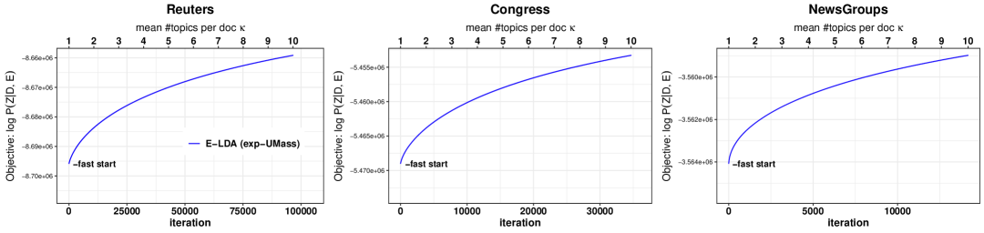
(a) Convergence of E-LDA’s objective values using the exp-UMass topic generator.

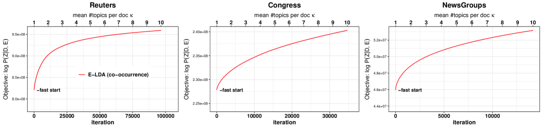
(b) Convergence using the co-occurrence topic generator.

Figure 3: Convergence of E-LDA’s objective values $\dot{f}$ using the (top row) exp-UMass topic generator and the (bottom row) co-occurrence topic generator.

Experiments Set 1: Objective values over multiple experimental runs. Table 2 reprints the $\dot{f}$ values from Experiments Set 1 with standard deviations added in parentheses. We excluded these from the body of the paper in the interest of making each baseline’s $\dot{f}$ values visually easier to compare across the table. For each baseline (Gibbs, Gibbs-Bayes, Gibbs-Sparse), E-LDA’s objective values are higher for all $90$ experiments, and the difference for each benchmark and each dataset is statistically significant at the $p$$<10^{-10}$ level per standard $2$-sided t-tests.

Experiments Set 2: evaluating the semantic quality of learned topics. In Experiments Set 2, we are interested in comparing the semantic quality of topics generated by E-LDA to those generated by state-of-the-art Gibbs-based LDA solvers. We measure topic quality via the widely-used UMass coherence measure [Mimno et al., 2011, Röder et al., 2015]. Recall that UMass coherence measures the (log) probability that the top (i.e. highest-probability) $h^{*}$ words in a topic co-appear in documents in the corpus. Specifically, for a given topic $\tau$, the normalized coherence is:

$$C(\tau,h^{*})=\frac{2}{h^{*}(h^{*}-1)}\sum_{h=2}^{h^{*}}\sum_{\ell=1}^{h-1}\log\frac{|D_{\tau_{h},\tau_{\ell}}|+\epsilon}{|D_{\tau_{\ell}|}}$$ (19)

where $D_{\tau_{h}}$ is the set of documents that contain the $h$’th most probable word according to topic $\tau$, $D_{\tau_{h},\tau_{\ell}}$ is the set that contain both the $h$’th and $\ell$’th most probable words according to topic $\tau$, and $\epsilon$ is a small constant that precludes the $\log(0)$ case. We choose the normalized variant that includes the $\frac{2}{h^{*}(h^{*}-1)}\sum_{h=2}^{h^{*}}$ factor because it render coherence scores comparable across different choices of $h^{*}$, as in Figs. 2(a) ($x$-axes).

Experiments Set 2: Baseline coherence variation over multiple runs. FastGreedy-E-LDA is deterministic, so its performance is always consistent across multiple runs. In contrast, Gibbs baselines’ solution quality varies from one run to the next. Fig. 4 reprints the main Gibbs baseline’s mean coherence scores from Fig 2(a) with added error bars showing its best and worst mean-coherence-per-run over $10$ re-runs to show the range of its typical performance. Observe that even by re-running the baseline $10$ times, no single run obtains coherence comparable to either of the E-LDA solutions.

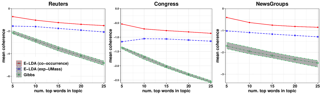
Figure 4: We reprint the main Gibbs baseline from Experiments Set 2 (Fig 2(a)) with added error bars showing its best and worst mean-coherence-per-run over the $10$ experimental runs.

Experiments Set 2: Additional baselines. For topic coherence experiments (Set $2$), we add recent neural and LLM-based baselines: BERTopic [Grootendorst, 2022], AVITM [Srivastava and Sutton, 2017], ETM [Dieng et al., 2020], and FASTopic [Wu et al., 2024b]. We use the authors’ codebases for each of these baselines (note that ETM and AVITM are now integrated with the OCTIS library [Terragni et al., 2021], and FASTopic is now integrated with the Topmost library [Wu et al., 2024c], and we set all parameters to be identical to the parameters in their respective papers. In terms of performance, ETM is the best-performing baseline. This matches expectations, as ETM was explicitly designed as a coherence-improving algorithm per [Dieng et al., 2020] (see also, e.g., Wu et al. [2024a]). We note that AVITM’s poor coherence matches anecdotal experience that this algorithm obtains good coherence on some datasets but requires customized parameter tuning to obtain competitive performance on others.

Scale of experiments. We note that the largest submodular problems in the literature are social network problems with ground sets of $\sim$$10^{7}$ elements. Our experiments described above consider $>10^{8}$ links. See Breuer et al. [2020], Mirzasoleiman et al. [2013], and Guestrin et al. [2005].

Appendix Q Deferred discussion of unmodified UMass topic generator

We include the UMass topic generator both to build intuition, and also because its poor post-hoc coherence scores provide a clear illustration that other topic generators are not obtaining high post-hoc coherence merely due to their similarity with the UMass coherence function. In particular, we note that the unmodified UMass generator produces topics that each assign probability mass too uniformly across the vocabulary, resulting in un-sparse topics with unfocused semantic meaning. We note that a comparable property is referred to as ”topic collapsing” when it arises in the context of recent neural topic modeling algorithms [Wu et al., 2023].

To be clear, post-hoc coherence scores only weigh the ranking of words in a topic according to their probability mass, so order-preserving transformations of topic distributions have no effect on a topic’s post-hoc coherence. Thus, the generated set of candidate topics using the UMass generator has the same coherence score as exp-UMass and Co-occurrence topics. However, UMass’s too-uniform topics cause our algorithm to do a poor job of selecting (for each document) a small, diverse set of focused topics that each well-represent a subset of the document’s words. This explains why the exponential transformations in exp-UMass and Co-occurrence produce much more focused topics, and also why the solution set of topics using these generators has far better post-hoc coherence scores than alternatives.

Appendix R Co-occurrence vs. exp-UMass topic generators in practice

We briefly note some practical experiences with the results of using co-occurrence vs. exp-UMass topic generators. Because co-occurrence favors topics associated with rigorous topic labels $w^{*}$ that are more popular, this results in fewer unique topics overall, and in topics that are more focused on familiar/popular concepts. In contrast, using exp-UMass topics tends to result in solutions that reflect more subtlety, including a wider variety of topics and less-common topic labels $w^{*}$. In practice, we prefer to use co-occurrence as a ‘first cut’ to familiarize ourselves with an unknown dataset, and then to apply exp-UMass to tease out subtler meanings for final analysis.

Appendix S Interpretability & simulateability: Additional discussion

We briefly note a separate interpretability advantage of our approach that is particularly relevant to practitioners working on problem instances in social science and causal inference. Specifically, because all mainstream topic modeling algorithms are gradient-based, their routines are too complex for a human researcher to vet. Put differently, a practitioner cannot look into the algorithm’s operations to obtain an answer to the question “Why did the algorithm assign the ‘physics’ topic to this document?”. This aspect of interpretability is variously referred to as ‘simulateability’ [Lipton, 2018]. We note that this problem is also a focal point of recent social science methodology discussions—see, e.g., Grimmer et al. [2022], Ying et al. [2022], and Ke et al. [2024].

In contrast, our Greedy-based algorithms are intuitively familiar to the human process of connecting topics to documents. Therefore, it is easy to answer such a question for a solution obtained by our algorithms. For example, the answer will be “The ‘physics’ topic was assigned to this document because it most improved the description of the document, which was previously described only by ‘space’ and ‘particle’ topics (i.e. the topics that were linked in $E_{d}$ before ‘physics’).” By ‘most improved’, we mean that the ‘physics’ topic offered the greatest increase in the probability of that document’s words compared to all remaining topics.

References

- Anandkumar et al. (2012) Anima Anandkumar, Dean P Foster, Daniel J Hsu, Sham M Kakade, and Yi-Kai Liu. A spectral algorithm for latent dirichlet allocation. Advances in neural information processing systems, 25, 2012.
- Arora et al. (2012) Sanjeev Arora, Rong Ge, and Ankur Moitra. Learning topic models–going beyond svd. In 2012 IEEE 53rd annual symposium on foundations of computer science, pages 1–10. IEEE, 2012.
- Arora et al. (2013) Sanjeev Arora, Rong Ge, Yonatan Halpern, David Mimno, Ankur Moitra, David Sontag, Yichen Wu, and Michael Zhu. A practical algorithm for topic modeling with provable guarantees. In International conference on machine learning, pages 280–288. PMLR, 2013.
- Arora et al. (2016a) Sanjeev Arora, Rong Ge, Ravi Kannan, and Ankur Moitra. Computing a nonnegative matrix factorization—provably. SIAM Journal on Computing, 45(4):1582–1611, 2016a.
- Arora et al. (2016b) Sanjeev Arora, Rong Ge, Frederic Koehler, Tengyu Ma, and Ankur Moitra. Provable algorithms for inference in topic models. In International Conference on Machine Learning, pages 2859–2867. PMLR, 2016b.
- Arora et al. (2018) Sanjeev Arora, Rong Ge, Yoni Halpern, David Mimno, Ankur Moitra, David Sontag, Yichen Wu, and Michael Zhu. Learning topic models provably and efficiently. volume 61, pages 85–93. ACM, 2018.
- Ash and Hansen (2023) Elliott Ash and Stephen Hansen. Text algorithms in economics. Annual Review of Economics, 15(1):659–688, 2023.
- Askari et al. (2020) Armin Askari, Alexandre d’Aspremont, and Laurent El Ghaoui. Naive feature selection: Sparsity in naive bayes. In International Conference on Artificial Intelligence and Statistics, pages 1813–1822. PMLR, 2020.
- Balkanski and Singer (2018) Eric Balkanski and Yaron Singer. The adaptive complexity of maximizing a submodular function. In Proceedings of the 50th annual ACM SIGACT symposium on theory of computing, pages 1138–1151, 2018.
- Balkanski et al. (2019) Eric Balkanski, Aviad Rubinstein, and Yaron Singer. An optimal approximation for submodular maximization under a matroid constraint in the adaptive complexity model. In Proceedings of the 51st Annual ACM SIGACT Symposium on Theory of Computing, pages 66–77, 2019.
- Barberá et al. (2019) Pablo Barberá, Andreu Casas, Jonathan Nagler, Patrick J Egan, Richard Bonneau, John T Jost, and Joshua A Tucker. Who leads? who follows? measuring issue attention and agenda setting by legislators and the mass public using social media data. American Political Science Review, 113(4):883–901, 2019.
- Battaglia et al. (2024) Laura Battaglia, Timothy Christensen, Stephen Hansen, and Szymon Sacher. Inference for regression with variables generated by ai or machine learning. arXiv preprint arXiv:2402.15585, 2024.
- Blanes i Vidal et al. (2012) Jordi Blanes i Vidal, Mirko Draca, and Christian Fons-Rosen. Revolving door lobbyists. The American Economic Review, 102(7):3731, 2012.
- Blei et al. (2003) David M Blei, Andrew Y Ng, and Michael I Jordan. Latent dirichlet allocation. Journal of machine Learning research, 3(Jan):993–1022, 2003.
- Breuer et al. (2020) Adam Breuer, Eric Balkanski, and Yaron Singer. The fast algorithm for submodular maximization. In International Conference on Machine Learning, pages 1134–1143. PMLR, 2020.
- Bybee et al. (2024) Leland Bybee, Bryan Kelly, Asaf Manela, and Dacheng Xiu. Business news and business cycles. The Journal of Finance, 79(5):3105–3147, 2024.
- Catalinac (2016) Amy Catalinac. From pork to policy: The rise of programmatic campaigning in Japanese elections. The Journal of Politics, 78(1):1–18, 2016.
- Chang et al. (2009) Jonathan Chang, Sean Gerrish, Chong Wang, Jordan Boyd-Graber, and David Blei. Reading tea leaves: How humans interpret topic models. Advances in neural information processing systems, 22, 2009.
- Chekuri and Quanrud (2019) Chandra Chekuri and Kent Quanrud. Submodular function maximization in parallel via the multilinear relaxation. SODA, 2019.
- Chib (1995) Siddhartha Chib. Marginal likelihood from the gibbs output. Journal of the American statistical association, 90(432):1313–1321, 1995.
- Dieng et al. (2020) Adji B Dieng, Francisco JR Ruiz, and David M Blei. Topic modeling in embedding spaces. Transactions of the Association for Computational Linguistics, 8:439–453, 2020.
- Dietrich et al. (2019) Bryce J Dietrich, Matthew Hayes, and Diana Z O’brien. Pitch perfect: Vocal pitch and the emotional intensity of congressional speech. American Political Science Review, 113(4):941–962, 2019.
- Djourelova (2023) Milena Djourelova. Persuasion through slanted language: Evidence from the media coverage of immigration. American economic review, 113(3):800–835, 2023.
- Doshi-Velez et al. (2015) Finale Doshi-Velez, Byron C Wallace, and Ryan Adams. Graph-sparse lda: a topic model with structured sparsity. In Twenty-Ninth AAAI conference on artificial intelligence, 2015.
- Egami et al. (2022) Naoki Egami, Christian J Fong, Justin Grimmer, Margaret E Roberts, and Brandon M Stewart. How to make causal inferences using texts. Science Advances, 8(42):eabg2652, 2022.
- Ene et al. (2019) Alina Ene, Huy L Nguyen, and Adrian Vladu. Submodular maximization with matroid and packing constraints in parallel. STOC, 2019.
- Eshima et al. (2020) Shusei Eshima, Kosuke Imai, and Tomoya Sasaki. Keyword assisted topic models. arXiv preprint arXiv:2004.05964, 2020.
- Fahrbach et al. (2019) Matthew Fahrbach, Vahab Mirrokni, and Morteza Zadimoghaddam. Submodular maximization with optimal approximation, adaptivity and query complexity. SODA, 2019.
- Feder et al. (2021) Amir Feder, Nadav Oved, Uri Shalit, and Roi Reichart. Causalm: Causal model explanation through counterfactual language models. Computational Linguistics, 47(2):333–386, 2021.
- Feder et al. (2022) Amir Feder, Katherine A Keith, Emaad Manzoor, Reid Pryzant, Dhanya Sridhar, Zach Wood-Doughty, Jacob Eisenstein, Justin Grimmer, Roi Reichart, Margaret E Roberts, et al. Causal inference in natural language processing: Estimation, prediction, interpretation and beyond. Transactions of the Association for Computational Linguistics, 10:1138–1158, 2022.
- Fong and Grimmer (2016) Christian Fong and Justin Grimmer. Discovery of treatments from text corpora. In Proceedings of the 54th Annual Meeting of the Association for Computational Linguistics (Volume 1: Long Papers), pages 1600–1609, 2016.
- Fong and Grimmer (2023) Christian Fong and Justin Grimmer. Causal inference with latent treatments. American Journal of Political Science, 67(2):374–389, 2023.
- Gerlach et al. (2018) Martin Gerlach, Tiago P Peixoto, and Eduardo G Altmann. A network approach to topic models. Science advances, 4(7):eaaq1360, 2018.
- Gomes and Krause (2010) Ryan Gomes and Andreas Krause. Budgeted nonparametric learning from data streams. In ICML, volume 1, page 3. Citeseer, 2010.
- Griffiths and Steyvers (2004) Thomas L Griffiths and Mark Steyvers. Finding scientific topics. Proceedings of the National academy of Sciences, 101(suppl 1):5228–5235, 2004.
- Grimmer et al. (2022) Justin Grimmer, Margaret E Roberts, and Brandon M Stewart. Text as data: A new framework for machine learning and the social sciences. Princeton University Press, 2022.
- Grootendorst (2022) Maarten Grootendorst. Bertopic: Neural topic modeling with a class-based tf-idf procedure. arXiv preprint arXiv:2203.05794, 2022.
- Guestrin et al. (2005) Carlos Guestrin, Andreas Krause, and Ajit Paul Singh. Near-optimal sensor placements in gaussian processes. In Proceedings of the 22nd international conference on Machine learning, pages 265–272, 2005.
- Hall et al. (2008) David Hall, Dan Jurafsky, and Christopher D Manning. Studying the history of ideas using topic models. In Proceedings of the 2008 conference on empirical methods in natural language processing, pages 363–371, 2008.
- Hu and Li (2021) Zhiting Hu and Li Erran Li. A causal lens for controllable text generation. Advances in Neural Information Processing Systems, 34:24941–24955, 2021.
- Iyer and Bilmes (2019) Rishabh Iyer and Jeffrey Bilmes. A memoization framework for scaling submodular optimization to large scale problems. In The 22nd International Conference on Artificial Intelligence and Statistics, pages 2340–2349. PMLR, 2019.
- Ke et al. (2024) Zheng Tracy Ke, Pengsheng Ji, Jiashun Jin, and Wanshan Li. Recent advances in text analysis. Annual Review of Statistics and Its Application, 11(1):annurev, 2024.
- Khanna et al. (2017) Rajiv Khanna, Ethan Elenberg, Alex Dimakis, Sahand Negahban, and Joydeep Ghosh. Scalable greedy feature selection via weak submodularity. In Artificial Intelligence and Statistics, pages 1560–1568. PMLR, 2017.
- Lang (1995) Ken Lang. Newsweeder: Learning to filter netnews. In Machine learning proceedings 1995, pages 331–339. Elsevier, 1995.
- Lau et al. (2014) Jey Han Lau, David Newman, and Timothy Baldwin. Machine reading tea leaves: Automatically evaluating topic coherence and topic model quality. In Proceedings of the 14th Conference of the European Chapter of the Association for Computational Linguistics, pages 530–539, 2014.
- Lauderdale and Clark (2014) Benjamin E Lauderdale and Tom S Clark. Scaling politically meaningful dimensions using texts and votes. American Journal of Political Science, 58(3):754–771, 2014.
- Lewis (1997) David Lewis. Reuters-21578 text categorization test collection. Distribution 1.0, AT&T Labs-Research, 1997.
- Li and McCallum (2006) Wei Li and Andrew McCallum. Pachinko allocation: Dag-structured mixture models of topic correlations. In Proceedings of the 23rd international conference on Machine learning, pages 577–584, 2006.
- Lin and Bilmes (2011) Hui Lin and Jeff Bilmes. A class of submodular functions for document summarization. In Proceedings of the 49th annual meeting of the association for computational linguistics: human language technologies, pages 510–520, 2011.
- Lindgren et al. (2016) Erik Lindgren, Shanshan Wu, and Alexandros G Dimakis. Leveraging sparsity for efficient submodular data summarization. Advances in Neural Information Processing Systems, 29, 2016.
- Lipton (2018) Zachary C Lipton. The mythos of model interpretability: In machine learning, the concept of interpretability is both important and slippery. Queue, 16(3):31–57, 2018.
- Liu et al. (2013) Ming-Yu Liu, Oncel Tuzel, Srikumar Ramalingam, and Rama Chellappa. Entropy-rate clustering: Cluster analysis via maximizing a submodular function subject to a matroid constraint. IEEE Transactions on Pattern Analysis and Machine Intelligence, 36(1):99–112, 2013.
- Madiega (2021) Tambiama Madiega. Artificial intelligence act. European Parliament: European Parliamentary Research Service, 2021.
- Martin and McCrain (2019) Gregory J Martin and Joshua McCrain. Local news and national politics. American Political Science Review, 113(2):372–384, 2019.
- (55) Andrew Kachites McCallum. Mallet: A machine learning for languagetoolkit. http://mallet. cs. umass. edu.
- Mimno et al. (2011) David Mimno, Hanna Wallach, Edmund Talley, Miriam Leenders, and Andrew McCallum. Optimizing semantic coherence in topic models. In Proceedings of the 2011 conference on empirical methods in natural language processing, pages 262–272, 2011.
- Minoux (1978) Michel Minoux. Accelerated greedy algorithms for maximizing submodular set functions. In Optimization techniques, pages 234–243. Springer, 1978.
- Mirzasoleiman et al. (2013) Baharan Mirzasoleiman, Amin Karbasi, Rik Sarkar, and Andreas Krause. Distributed submodular maximization: Identifying representative elements in massive data. In Advances in Neural Information Processing Systems, pages 2049–2057, 2013.
- Mirzasoleiman et al. (2015) Baharan Mirzasoleiman, Ashwinkumar Badanidiyuru, Amin Karbasi, Jan Vondrák, and Andreas Krause. Lazier than lazy greedy. In Twenty-Ninth AAAI Conference on Artificial Intelligence, 2015.
- Mirzasoleiman et al. (2016) Baharan Mirzasoleiman, Ashwinkumar Badanidiyuru, and Amin Karbasi. Fast constrained submodular maximization: Personalized data summarization. In ICML, pages 1358–1367, 2016.
- Modarressi et al. (2025) Iman Modarressi, Jann Spiess, and Amar Venugopal. Causal inference on outcomes learned from text. arXiv preprint arXiv:2503.00725, 2025.
- Mueller and Rauh (2018) Hannes Mueller and Christopher Rauh. Reading between the lines: Prediction of political violence using newspaper text. American Political Science Review, 112(2):358–375, 2018.
- Nemhauser and Wolsey (1978) George L Nemhauser and Laurence A Wolsey. Best algorithms for approximating the maximum of a submodular set function. Mathematics of operations research, 3(3):177–188, 1978.
- Nemhauser et al. (1978) George L Nemhauser, Laurence A Wolsey, and Marshall L Fisher. An analysis of approximations for maximizing submodular set functions—i. Mathematical Programming, 14(1):265–294, 1978.
- Newton and Raftery (1994) Michael A Newton and Adrian E Raftery. Approximate bayesian inference with the weighted likelihood bootstrap. Journal of the Royal Statistical Society Series B: Statistical Methodology, 56(1):3–26, 1994.
- Pan and Chen (2018) Jennifer Pan and Kaiping Chen. Concealing corruption: How chinese officials distort upward reporting of online grievances. The American Political Science Review, 112(3):602–620, 2018.
- Pearl (2009) Judea Pearl. Causality. Cambridge university press, 2009.
- Pokutta et al. (2020) Sebastian Pokutta, Mohit Singh, and Alfredo Torrico. On the unreasonable effectiveness of the greedy algorithm: Greedy adapts to sharpness. In International Conference on Machine Learning, pages 7772–7782. PMLR, 2020.
- Qian and Singer (2019) Sharon Qian and Yaron Singer. Fast parallel algorithms for statistical subset selection problems. In Advances in Neural Information Processing Systems, pages 5073–5082, 2019.
- Röder et al. (2015) Michael Röder, Andreas Both, and Alexander Hinneburg. Exploring the space of topic coherence measures. In Proceedings of the eighth ACM international conference on Web search and data mining, pages 399–408, 2015.
- Rubin (1974) Donald B Rubin. Estimating causal effects of treatments in randomized and nonrandomized studies. Journal of educational Psychology, 66(5):688, 1974.
- Rubin (1980) Donald B Rubin. Randomization analysis of experimental data: The fisher randomization test comment. Journal of the American statistical association, 75(371):591–593, 1980.
- Sontag and Roy (2011) David Sontag and Dan Roy. Complexity of inference in latent dirichlet allocation. Advances in neural information processing systems, 24, 2011.
- Srivastava and Sutton (2017) Akash Srivastava and Charles Sutton. Autoencoding variational inference for topic models. arXiv preprint arXiv:1703.01488, 2017.
- Terragni et al. (2021) Silvia Terragni, Elisabetta Fersini, Bruno Giovanni Galuzzi, Pietro Tropeano, and Antonio Candelieri. Octis: Comparing and optimizing topic models is simple! In Proceedings of the 16th Conference of the European Chapter of the Association for Computational Linguistics: System Demonstrations, pages 263–270, 2021.
- Thomas et al. (2006) Matt Thomas, Bo Pang, and Lillian Lee. Get out the vote: determining support or opposition from congressional floor-debate transcripts. In Proceedings of the 2006 Conference on Empirical Methods in Natural Language Processing, pages 327–335, 2006.
- Tingley (2017) Dustin Tingley. Rising power on the mind. International Organization, pages S165–S188, 2017.
- Veitch et al. (2020) Victor Veitch, Dhanya Sridhar, and David Blei. Adapting text embeddings for causal inference. In Conference on Uncertainty in Artificial Intelligence, pages 919–928. PMLR, 2020.
- Wallach et al. (2009a) Hanna Wallach, David Mimno, and Andrew McCallum. Rethinking lda: Why priors matter. Advances in neural information processing systems, 22, 2009a.
- Wallach et al. (2009b) Hanna M Wallach, Iain Murray, Ruslan Salakhutdinov, and David Mimno. Evaluation methods for topic models. In Proceedings of the 26th annual international conference on machine learning, pages 1105–1112, 2009b.
- Wallach (2008) Hanna Megan Wallach. Structured topic models for language. PhD thesis, University of Cambridge Cambridge, UK, 2008.
- Wu et al. (2023) Xiaobao Wu, Xinshuai Dong, Thong Thanh Nguyen, and Anh Tuan Luu. Effective neural topic modeling with embedding clustering regularization. In International Conference on Machine Learning, pages 37335–37357. PMLR, 2023.
- Wu et al. (2024a) Xiaobao Wu, Thong Nguyen, and Anh Tuan Luu. A survey on neural topic models: methods, applications, and challenges. Artificial Intelligence Review, 57(2):18, 2024a.
- Wu et al. (2024b) Xiaobao Wu, Thong Nguyen, Delvin Zhang, William Yang Wang, and Anh Tuan Luu. Fastopic: Pretrained transformer is a fast, adaptive, stable, and transferable topic model. Advances in Neural Information Processing Systems, 37:84447–84481, 2024b.
- Wu et al. (2024c) Xiaobao Wu, Fengjun Pan, and Luu Anh Tuan. Towards the topmost: A topic modeling system toolkit. In Proceedings of the 62nd Annual Meeting of the Association for Computational Linguistics (Volume 3: System Demonstrations), pages 31–41, 2024c.
- Ying et al. (2022) Luwei Ying, Jacob M Montgomery, and Brandon M Stewart. Topics, concepts, and measurement: A crowdsourced procedure for validating topics as measures. Political Analysis, 30(4):570–589, 2022.