Interface Fragmentation via Horizontal Vibration: A Pathway to Scalable Monodisperse Emulsification

Abstract

We present a scalable method for producing monodisperse microscale emulsions in a container holding two stably stratified layers of immiscible liquids by applying horizontal vibration. Our experiments and theoretical modelling show that the critical non-dimensional acceleration for regular droplet formation is governed by a shear-dominated breakup mechanism, which scales as $N^{-1/2}\omega^{*3/2}$, where $N$ is the viscosity ratio and $\omega^{*}$ is the frequency of forcing on the viscous-capillary scale. The droplet diameter can be easily controlled by varying the forcing parameters, thus demonstrating this vibrational configuration as a scalable alternative to microfluidics.

Emulsification, a powerful technique for dispersing a liquid in a second immiscible phase, underpins a wide range of practical applications from food processing [1] and drug delivery systems [2, 3] to solvent extraction [4]. Although the processes used in these applications are different, they typically demand precise control of the emulsion properties. For example, droplet size and production rate are key determinants of the mass transfer rate of the solvent to be extracted using emulsion-liquid-membrane technology in wastewater treatment [5]. However, controlling emulsification at application scale remains a significant technical challenge.

The fundamental route to droplet formation is through the fragmentation of a liquid interface subject to shear or impact stresses [6, 7]. Primary instabilities give rise to corrugated liquid threads or ligaments, whose breakup in turn determines the drop-size distribution. Polydispersity stems principally from the dynamics and fragmentation of these ligaments, including phenomena such as ligament-turbulence interactions, satellite drop ejection, and subsequent coalescence events—all of which are difficult to control due to their sensitivity to local flow conditions and interfacial instabilities.

Rotor stators and homogenisers provide “top-down” high-energy methods of emulsification [8], where fluctuations in local shear stress across the system result in compositional heterogeneity [9, 10]. These methods suit large-scale production but offer little control over individual droplet formation, resulting in a broad size distribution of the dispersed phase. To improve control over droplet size and size variation, controlled-shear emulsification techniques, such as membrane emulsification [11] and microfluidic methods [12] have gained momentum over the past two decades [13]. The latter provides a “bottom-up” approach to emulsification via the production of droplets of tuneable size from controlled interface break-up in confined flow geometries, e.g., Y or T-junctions, co-flowing, flow-focusing or cross-flow configurations [14, 15, 13, 16, 17, 18], as well as in ”chip-free” microfluidic systems [19, 20] . Furthermore, tuneable interfacial tension has recently been used to reconfigure complex emulsions dynamically [21]. However, although microfluidic devices can achieve upscaled production of monodisperse emulsion through parallelization [13], they rarely provide a viable option for practical applications because of their high cost of installation and maintenance [22].

Figure 1: (a) Schematic diagram of the experimental set-up. The blue rectangle shows a close-up snapshot of subharmonic waves localised near the right end wall captured in angled top-view. The pink arrow indicates subharmonic wave tips and the orange arrow points to the edge of the subharmonic waves below the onset of droplet formation, which occurs at the threshold amplitude $A_{c}$. (b) Top-view image of the formation of regular droplet trains at the end wall (see Movie 1 in Supplemental Materials [23]). (c) Different vibrational parameters generate droplets of different size, visualized from in angled top-view (end wall indicated by yellow line).

In this letter, we propose an alternative scalable method for the production of monodisperse droplets with tuneable size, by harnessing an interfacial instability that arises near the end walls of a horizontally vibrated vessel containing two layers of immiscible liquids. Horizontal vibration differentially accelerates two superposed, immiscible fluid layers confined by end walls into a counterflow [24, 25], thus providing an alternative strategy for controlling shear in the context of interface fragmentation. An advantage of this method is that we can generate on-demand stabilizer-free emulsions through external forcing, which are sustained under vibration but rapidly return to separated phases upon interruption of the forcing. Alternatively, the emulsion may be stabilized by introducing surfactants [9, 12] for use after vibration cessation. We establish universal scalings for the vibrational parameters required for onset of droplets and identify a regime for monodisperse droplet formation and associated scalings to predict droplet size.

We performed experiments in a sealed rectangular Perspex container with inner dimensions of $170\times 75\times 40\,\mathrm{mm}^{3}$ containing two stably stratified, immiscible liquids of equal volume; see Fig.1(a). For the upper layer, we used four grades of silicone oils (polydimethylsiloxane fluid, 10 cS, 20 cS, 50 cS, 100 cS, Basildon Chemicals Ltd) and for the lower layer, two perfluorinated polyethers (Galden^® HT135 and HT270, Solvay), with respective densities, $\rho_{\mathrm{u}}$, $\rho_{\mathrm{l}}$, and viscosities, $\nu_{\mathrm{u}}$, $\nu_{\mathrm{l}}$ listed in . In this letter, we show that monodisperse droplet formation is governed by the viscosity ratio $N=\nu_{\mathrm{u}}/\nu_{\mathrm{l}}$, and thus we will use this parameter to identify the fluid pairs.

The container was subject to horizontal harmonic oscillations imposed with a horizontal vibration system, with a prescribed velocity $A\omega\cos(\omega t)$, where the amplitude, $A$, and the angular frequency, $\omega=2\pi F$, varied in the ranges $A\leq 3.50$ mm and $20\,\mathrm{Hz}\leq F\leq 60\,\mathrm{Hz}$ (see End Matter for technical specifications). We imaged the interface dynamics in the near-endwall region (orange rectangle in Fig.1(a)) with a high-speed camera (Photron FASTCAM mini AX100) and a CMOS camera (Teledyne DALSA Inc, Genie HC1400). The Photron camera was used to capture time-resolved images in top view and angled top view (Fig.1(a)), with respective resolutions of 15.1 and 48.8 pixels/mm and a minimum rate of 4000 frames per second (fps). The droplet formation was monitored by recording top-view movies at 10 fps with the Dalsa Genie camera with a maximum resolution of 75.4 pixels/mm. The interface was visible due to the difference in refractive indices between the two liquid layers. We extracted the wavenumber $k=2\pi/\lambda$ of the interfacial instability, where $\lambda$ is the wavelength of the periodic interface deformation, and the diameter of the droplet $D$ from raw images using image processing, see End Matter for details.

Figure 2: (a-c) Experimental snapshots of three distinguished types of interfacial breakups: (a) breakup Ia in $N$=9.2, (b) breakup Ib and (c) breakup II, both in $N$=48.9. Red and blue boxes in (c) highlight the snapshots before and after interface disintegration. (d) Schematic illustration of the representative breakup mechanisms. Red and blue arrows indicate fluid velocity directions in the upper and lower layers, respectively. Blue and red dots indicate the container reaches its far-left and far-right positions (see Fig.A2(a) in the End Matter).

Figure 3: (a) Critical acceleration measured with different forcing frequencies $F$ and viscous ratios $N$, marked with different symbols. (b) Log-Log plot of non-dimensional acceleration vs non-dimensional frequency. The linear regression yields $a_{\mathrm{c}}^{*}\sim\omega^{*1.498\pm 0.007}$ (solid line) and $a_{\mathrm{c}}^{*}\sim\omega^{*1.336\pm 0.004}$(dashed line), respectively. $\omega_{\mathrm{int}}$ denotes the intersection point of the two lines. (c) The ratio of interfacial Stoke boundary layer thickness to the onset wavelength $\delta/\lambda_{\mathrm{c}}$ plotted against non-dimensional frequency, where $\omega_{r}^{*}$ marks the location of which $\delta/\lambda_{\mathrm{c}}\cong 0.16$.

Fig.1(a) shows a regular array of subharmonic standing waves which was excited near the end walls of the container via a Faraday instability, by incrementally increasing the forcing amplitude beyond a critical value [27]. The onset of waves occurs because the inertial counterflow induced by the differential acceleration of the fluid layers and the presence of end walls, redirects horizontal oscillatory forcing into vertical oscillation of a localised interfacial front, which becomes unstable at a critical value of forcing. However, a further small amplitude increase beyond the onset of subharmonic waves leads to onset of droplet detachment at a threshold value $A_{c}$. Droplet shedding occurs periodically from the crests of the subharmonic waves resulting in regular droplets trains of lower-layer liquid (Fig.1(b)) dispersing in the continuous upper layer liquid. The droplets in each train are approximately monodisperse, and their size can be adjusted by varying the amplitude and frequency of the applied horizontal forcing (Fig.1(c)).

However, we find that monodisperse droplet formation is not the norm, and that the nature of interfacial breakup varies significantly with variations of $N$, $F$ and $A$, as illustrated in the End Matter for fluid pairs with $N$=9.2 and 48.9 at different forcing frequencies. We observed three types of interfacial breakup (Ia, Ib, II) which each occur within different parameter ranges following the elongation into a ligament of the subharmonic wave tip made of lower-layer fluid, but only type II enables regular formation of monodisperse droplets. Figure 2 shows detailed time-sequences in angled top-view, of the elongation of the wave tip until breakup. The different types of interfacial breakup are distinguished by the orientation along which the wave tip elongates, as shown in the schematics of Fig.2(d). The green arrows indicate the thin liquid threads which result from the necking of the elongating ligaments, immediately prior to droplet detachment from the interface. These thin threads rupture as the external forcing transmitted through the motion of the upper liquid (EF) becomes sufficiently strong. Horizontal EF (along the $x$-axis) dominates the regular formation of monodisperse droplets associated with type II breakup (Fig.2(c)). In contrast, irregular droplet formation is associated with non-horizontal EF, where for type Ia (Fig.2(a)), the ligament orientation is close to vertical, and for type Ib (Fig.2(b)), it has both horizontal and vertical components.

To gain physical insight into these breakup mechanisms, we quantify in Fig. 3(a) the threshold acceleration of forcing, $a_{\mathrm{c}}=A_{\mathrm{c}}\omega^{2}$, beyond which droplets appear as a function of the forcing frequency for different fluid pairs. Measurements were made by imposing forcing frequency and gradually increasing the forcing amplitude in increments of 0.01 mm until the first appearance of droplets at the threshold amplitude $A_{c}$. We recorded at least 750 oscillation cycles to monitor the collection of droplets at onset (see Movie 2 in Supplemental Materials [23]) and ensured that all droplets coalesced back into the lower layer before taking the next measurement. The lower edge of the shaded bands marks the threshold for droplet formation near the end wall boundaries, while the upper edge indicates the threshold for droplet formation away from these boundaries. We find that the threshold acceleration increases monotonically with increasing forcing frequency for each fluid pair. The onset datasets are stacked sequentially in order of increasing viscosity ratio, with the bottom dataset corresponding to $N=9.2$ (HT135 & 10cS). For the fluid pair with the lowest $N=4.7$ (HT270 & 50cS), we did not observe droplet formation, only regular wall-confined subharmonic waves. The waves tips elongated into ligaments oriented horizontally, consistent with type II breakup (Fig.2(d)), but not sufficiently to cause rupture. This is because the ratio of the ligament breakup time ($\sim\lambda\rho_{\mathrm{l}}\nu_{\mathrm{l}}/\sigma$, where $\sigma$ is the interfacial tension ) [28, 29] to the timescale of EF ($\sim(\omega)^{-1}$) increases in proportion to the lower layer viscosity from $O(10^{-1})$ to $O(10^{0})$, when the fluid HT270 is used as the lower layer instead of HT135. Given the role of viscous forces in the upper layer on the breakup of the interface, we introduce a viscous-capillary length, $l_{\mathrm{vc}}=\nu_{\mathrm{u}}^{2}/(\sigma/\rho_{\mathrm{u}})$, and a viscous-capillary frequency, $\Omega_{\mathrm{vc}}=(\sigma/\rho_{\mathrm{u}})^{2}/(\nu_{\mathrm{u}}^{3})$ [30, 27], which we use to scale the critical acceleration, $a_{\mathrm{c}}^{*}=a_{\mathrm{c}}/(l_{\mathrm{vc}}\Omega_{\mathrm{vc}}^{2})$, and frequency, $\omega^{*}=\omega/\Omega_{\mathrm{vc}}$. The scaled data from Fig.3(a) collapses onto two distinct master curves in Fig.3(b), which cross over at approximately $\omega_{\mathrm{int}}^{*}\cong 0.19$. For $\omega^{*}\geq\omega_{\mathrm{int}}^{*}$, $a_{\mathrm{c}}^{*}\propto\omega^{*3/2}$ is associated with regular droplet formation of type II, while for $\omega^{*}<\omega_{\mathrm{int}}^{*}$, $a_{\mathrm{c}}^{*}\propto\omega^{*4/3}$, which indicates irregular droplet formation.

We can separate the different types of droplet formation more accurately along the $\omega^{*}$ axis in Fig. 3(c) by plotting as a function of $\omega^{*}$, the ratio of the interfacial Stokes boundary layer thickness of the upper layer, $\delta\equiv(2\nu_{u}/\omega)^{1/2}$ to the wavelength of the subharmonic waves at the onset of droplet formation, $\lambda_{\mathrm{c}}=2\pi/k_{\mathrm{c}}$. The symbols used to indicate different values of $N$ are the same as in Fig.3(a). Each data point represents the mean value obtained from several separate experiments, with the error bars indicating the corresponding standard deviation. We find that trains of regular droplets form only when the ratio $\delta/\lambda_{\mathrm{c}}$ is greater than about 0.16 where the non-dimensional forcing frequency, log$(\omega_{r}^{*})\approx-0.14$ ($\omega_{r}^{*}\approx 0.72$). This indicates that a thicker interfacial Stokes boundary layer is required in the upper layer to induce type II breakup. Thus, we suggest that breakup II is dominant for $\omega^{*}\geq\omega_{r}^{*}$ (‘regular region’), while for $\omega^{*}\leq\omega_{r}^{*}$ (‘irregular region’) type Ia and Ib breakups lead to the formation of irregular droplets in $\omega^{*}\leq\omega_{\mathrm{int}}^{*}$ and $\omega_{\mathrm{int}}^{*}<\omega^{*}<\omega_{r}^{*}$, respectively, as shown in Fig.3(c).

To understand the physics governing both irregular and regular interfacial breakup, we develop models of the elongated fluid ligament based on a simple force balance in the first case and an energy balance in the second, using suitable scaling arguments [30]. The model for type Ia breakup is based on the assumption of capillary instability [31]: as the wave tip with the most unstable wavelength $\lambda_{m}$ elongates into a thin ligament with a minimum diameter $d_{m}$ due to EF mediated by vertical shear forces in the upper fluid layer, the ligament can rupture when the viscous shear force overcomes the capillary restoring force. The capillary force per unit mass on the droplet-forming ligament with a mean diameter $d_{o}$ is $F_{\sigma}=\sigma\pi d_{o}/(\pi\rho_{l}d_{o}^{3}/6)$. The mean diameter is typically proportional to the most unstable wavelength, $d_{o}\sim\lambda_{m}$, which can be characterized by the onset wavelength ($\lambda_{c}$) at droplet formation [32, 30, 33, 34]. Hence, $F_{\sigma}\sim\sigma/(\rho_{l}\lambda_{c}^{2})$, where $\lambda_{c}=2\pi/k_{c}$ in the capillary limit is given by $\omega^{2}=4\sigma(k_{c})^{3}/(\rho_{l}+\rho_{u})$ [27]. The vertical shear force exerted by the fluid in the upper layer in the end wall region is estimated using the vibrational velocity $A\omega$ and the thickness of the Stokes layer $\delta$ such that $F_{V}=\nu_{u}\nabla^{2}u\sim\nu_{u}(A\omega)/(\delta)^{2}\sim A\omega^{2}$. The threshold for droplet detachment is $F_{V}\sim F_{\sigma}$ at $A=A_{\mathrm{c}}$. Hence, the critical acceleration on the viscous-capillary scale for the onset of type Ia breakup is given by

$$a_{\mathrm{c}}^{*}\sim(\rho_{u}/\rho_{l})^{1/3}{(\frac{\rho_{l}+\rho_{u}}{\rho_{l}}})^{2/3}\omega^{*4/3},$$ (1)

with a frequency dependence in $\omega^{*4/3}$ which matches our experimental observations of type Ia breakup (see Fig.3(b)).

Figure 4: Variation of non-dimensional droplet diameter $D^{*}$ with non-dimensional forcing amplitude $A^{*}$ for $N$=48.9 across different frequencies $F$ in the regular region. The solid line is a linear fit to the data. Inset: raw data of the droplet diameter vs forcing acceleration. Error bars denote the standard deviations of several separate measurements.

For type II breakup (Fig.2(d)), we argue that the energy received to create regular droplets ($E_{s}$) is set by the balance between the work of the horizontal shear force exerted by the upper layer fluid ($E$) and the energy dissipation due to the resistance to extension of the droplet-forming ligament. For fixed forcing, the constant rate of droplet production indicates that the rate of energy transfer to the droplet-forming ligament $\dot{E_{s}}$ is zero. Hence, the onset of regular droplet formation can be predicted by balancing the rate of work of the horizontal shear force and the rate of energy dissipation. The rate of work per unit mass can be written as $\dot{E}=F_{H}A\omega$, where $F_{H}\sim A\omega^{2}$ is the horizontal viscous shear force per unit mass which takes a form similar to $F_{V}$ above. The rate of energy dissipation per unit mass is generally estimated as $\varepsilon=\nu_{l}(u_{\mathrm{s}}/l)^{2}$, where $\nu_{l}$ is the kinematic viscosity of the droplet-forming ligament, $u_{\mathrm{s}}$ and $l$ represent the stretching velocity and length of the ligament, respectively [30, 34]. Using $\omega^{-1}$ as the time scale of the stretched ligament, the stretching velocity is $u_{\mathrm{s}}=l\omega$ and, thus, the energy dissipation rate is given by $\varepsilon\sim\nu_{l}\omega^{2}$ [30, 34]. Balancing $\dot{E}$ and $\varepsilon$ on the viscous-capillary scale yields an expression for the critical acceleration,

$$a_{\mathrm{c}}^{*}\sim(\nu_{l}/\nu_{u})^{1/2}\omega^{*3/2}=N^{-1/2}\omega^{*3/2},$$ (2)

with a frequency dependence in $\omega^{*3/2}$ which matches our experiments in the region of type II breakup (see Fig.3(b)). Expression (2) indicates that the threshold acceleration is governed by the viscosity ratio, rather than the viscosity of the upper fluid layer or the mean viscosity that governs the onset of subharmonic waves, as shown in Fig.3. This model also shows that for breakup II, the extensional viscous forces in the droplet-forming ligament dominate over capillary forces. We refer to this mechanism as a shear-dominated breakup. Type Ib breakup is likely caused by a more complex competition between inertia, capillary, viscous and gravitational forces (see Mechanism Ib in Fig.2(d)), which differs from type Ia and II breakups; a model for type Ib breakup is beyond the scope of this Letter.

We have shown that the onset wavelength and Stokes layer thickness dominate the size of the droplet-forming ligament and the effect of viscous shear forces in the upper fluid layer at the interface, respectively. Fig.4 shows the scaled droplet diameter, $D^{*}=D/\lambda_{c}$ as a function of the non-dimensional forcing amplitude, $A^{*}=A/\delta$ in the regular region. We find that all droplet diameter data collapse onto a straight line with a slope of $0.197\pm 0.015$, which we obtained by linear regression of the experimental data. We find that the smaller droplets form with larger $F$ and increasing acceleration at a fixed $F$ can monotonically increase the diameter of the droplet (see inset in Fig.4). Our measured minimum $D$ at $F$=50 Hz is about $167.0\pm 32.7$ µm. Note that the ratio of the standard deviation of the droplet diameter to the mean diameter is smaller than 25% in each dataset, which complies with a monodisperse criterion in emulsions [3].

In summary, we have studied the formation of a monodisperse emulsion in confined two-layer immiscible liquids subject to horizontal vibrations. Depending on the combined effect of the viscosity and forcing frequency, $\omega^{*}$, we have identified that monodisperse microscale emulsions are generated for $\omega^{*}\geq$ 0.72 through a shear-dominated breakup mechanism. The simple dependence of the non-dimensional droplet diameter on the non-dimensional forcing amplitude indicates that the diameter of monodisperse droplets can be easily controlled by adjusting the forcing frequency and amplitude. A key advantage of our method is that clogging, which is common in microfluidics [13, 22], can be avoided during the generation of monodisperse droplets. This means that parallelization can be used, e.g., by simultaneously vibrating multiple containers (increasing $N_{wall}$), to scale up production in practical applications while reducing installation and maintenance costs compared to microfluidics. The shear-induced instability we reveal may also offer new insights into the mechanisms underlying sea spray generation from breaking surface waves [35] and expiratory droplet formation during speech [36].

This research was supported by a Horizon Europe Guarantee MSCA Postdoctoral Fellowship through EPSRC (EP/X023176/1).

Appendix A End Matter

A.1 Horizontal vibration system

As illustrated in Fig. A1, the horizontal vibration system comprises a permanent magnet shaker (LDS-V450), a linear amplifier (LDS, PA1000L), a vibration controller (LDS-COMET USB), a laptop or PC, and a linear air-bearing slide. The container is rigidly mounted on a linear air-bearing slide, which is connected to the shaker via a steel driving shaft (a thin rod) with a diameter of 2 mm. Driven by a linear amplifier, the shaker imposes horizontal vibration on the container with a prescribed velocity. The harmonic content of the container’s motion, measured using a calibrated accelerometer (PCB Piezotronics, model 353B43), remained below 0.1% across the entire frequency range. This vibration system has previously been employed to investigate wave instabilities [24, 25, 27].

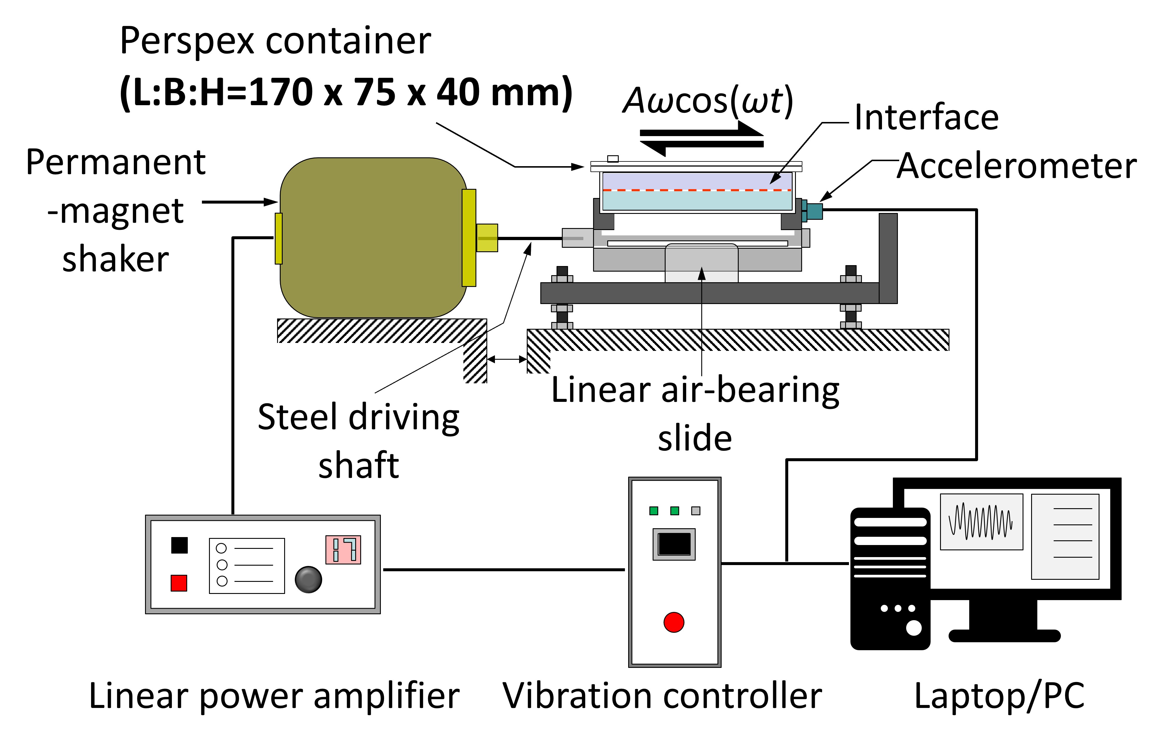
Figure A1: Schematic diagram of the horizontal vibration system.

A.2 Measurement of wavenumber and droplet diameter

To obtain precise wavenumber information, a pattern with 12 black lines parallel to the end walls was placed below the transparent bottom boundary of the container to assist measurements. The lines have a thickness of 0.2 mm and an interline spacing of 1 mm. The visualisation in top-view of the image of this line pattern, refracted by the fluid interface, enabled the detection of small interface deformations along the $y$-direction (Fig.1(a))) down to 0.1 mm, by measuring the distortion of the line. The wavenumber of the periodic deformation, $k=2\pi/\lambda=2\pi M/(W/2)$ [27], was determined by measuring $M$, the number of wavelengths ($\lambda$) spanning the half-width ($W/2$) of the container. $M$ was obtained by Fast Fourier Transform of the edge of the wave pattern along the $y$-direction tracked using MATLAB’s Canny algorithm.

The boundaries of dispersed droplets obtained from our experimental images exhibit strong contrast and clear definition. Therefore, we extracted the edge of the droplet and calculated its diameter $D=\frac{2}{J}\Sigma_{i=1}^{J}\sqrt{(x_{i}-x_{\mathrm{c}})^{2}+(y_{i}-y_{\mathrm{c}})^{2}}$, where $J$ is the number of edge points, ($x_{i},y_{i}$) the coordinates of an edge point and ($x_{\mathrm{c}},y_{\mathrm{c}}$) the centre of the droplet.

A.3 Regular versus irregular droplet formation

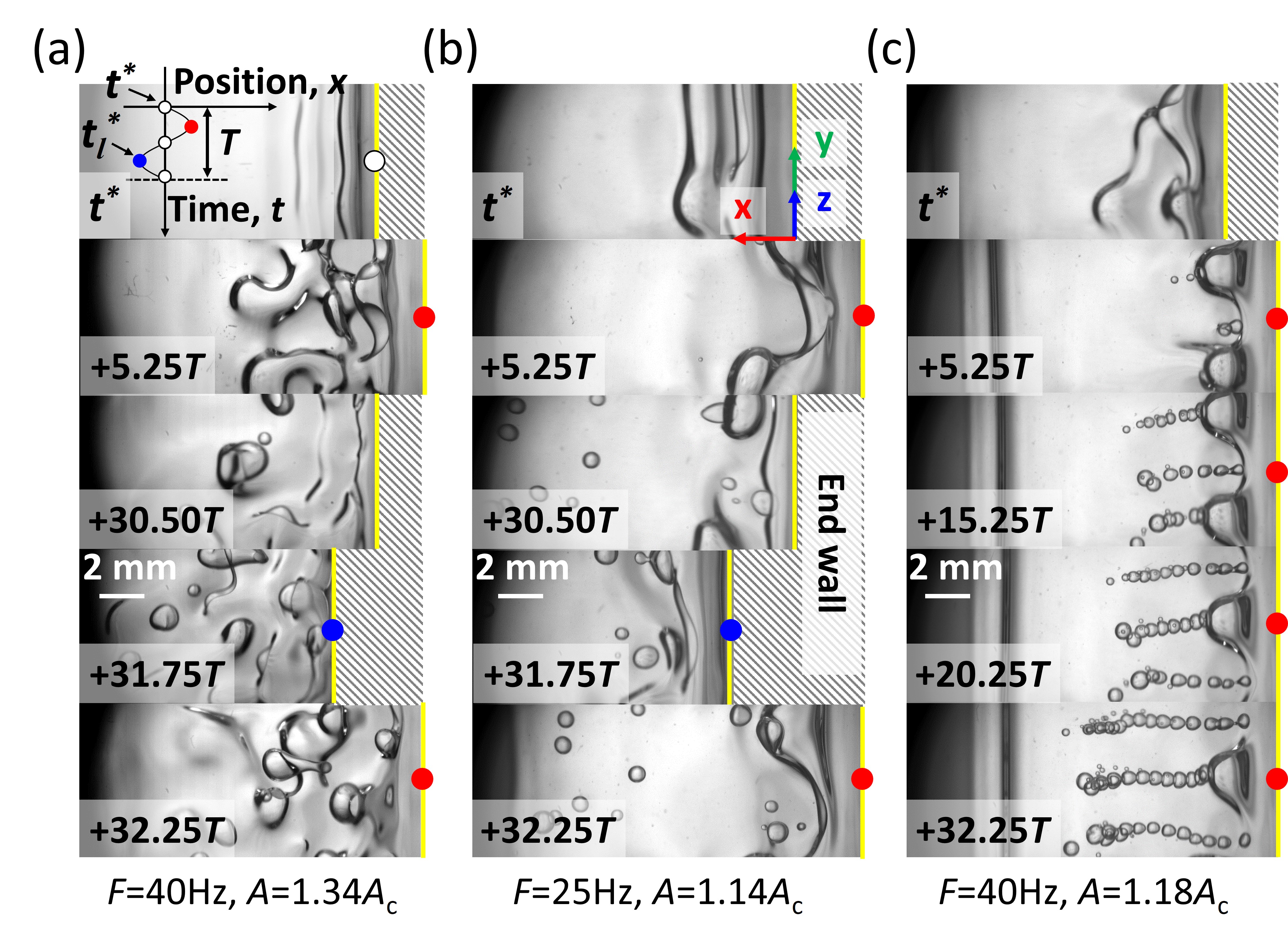
Figure A2: Representative images of droplet formation localised near the end walls under different forcing conditions and fluid pairs: (a) $N$=9.2 (HT135 & 10cS) and (b, c) $N$=48.9 (HT135 & 50cS). Inset in (a) shows a schematic of the container’s center x-position over one period. The $x$ displacement of the end wall (vertical yellow line) indicates the instantaneous displacement of the vessel. All images are shown in the angled top view (Fig.1(a)).

Regular versus irregular droplet formation is associated with the properties of the subharmonic waves excited near the end walls, which differ depending on the relative magnitude of viscous and capillary effects, imposed in our experiments by vibrational parameters and fluid viscosities [27]. In Fig.A2, we present angled top-view snapshots captured every quarter period across multiple cycles of oscillation. Fig.A2(a,b) shows that irregular interfacial breakup can occur for widely different values of $N$. Droplets form irregularly for $N$=9.2 regardless of forcing frequency, while for $N$=48.9 droplet formation is only irregular at moderate frequencies. For this more viscous system, an increase in forcing frequency yields a transition from irregular to regular droplet train formation (Fig.A2(b,c)). The snapshots in Fig.A2(c) indicate that droplets shed periodically from regular subharmonic waves form lines of droplet trains and move far away from the end wall. Hence, the production rate ($f_{\mathrm{p}}$) of regular droplets near each end wall is proportional to the vibration frequency for a fluid pair with a higher viscosity ratio, with $f_{p}=\frac{1}{2}FM$. Note that since the recording begins near $t$=0 when the vibration is first initiated, some early irregular droplets in Fig. A2(c) are attributed to the transient phase before the system reaches a stable oscillatory state. For less viscous fluid pairs or low frequencies of forcing, a slight increase in forcing amplitude beyond the onset of subharmonic waves suffices to generate wave interactions which yield irregular patterns spreading away from the end wall [27]. These irregular wave patterns in turn break up in a disorderly manner to produce strongly polydisperse droplets of uncontrolled size distribution.

References

- McClements [2004] D. J. McClements, Food Emulsions: Principles, Practices, and Techniques, Second Edition (CRC Press, 2004).
- Washington [1996] C. Washington, Adv. Drug Deliv. Rev. 20, 131 (1996).
- Ho et al. [2022] T. M. Ho, A. Razzaghi, A. Ramachandran, and K. S. Mikkonen, Adv. Colloid Interface Sci. 299, 102541 (2022).
- Ahmad et al. [2011] A. L. Ahmad, A. Kusumastuti, C. J. C. Derek, and B. S. Ooi, J. Chem. Eng. 171, 870 (2011).
- Kumar and Panesar [2019] A. Kumar, A.and Thakur and P. S. Panesar, Rev. Environ. Sci. Biotechnol. 18, 153 (2019).
- Villermaux [2007] E. Villermaux, Annu. Rev. Fluid Mech. 39, 419 (2007).
- Barrero and Loscertales [2007] A. Barrero and I. G. Loscertales, Annu. Rev. Fluid Mech. 39, 89 (2007).
- Håkansson [2019] A. Håkansson, Annu. Rev. Food Sc. Tech. 10, 239 (2019).
- Anna et al. [2003] S. L. Anna, N. Bontoux, and H. A. Stone, Appl. Phys. Lett. 82, 364 (2003).
- Evangelio et al. [2016] A. Evangelio, F. Campo-Cortés, and J. M. Gordillo, J. Fluid Mech. 804, 550 (2016).
- Meyer and Crocker [2009] R. F. Meyer and J. C. Crocker, Phys. Rev. Lett. 102, 194501 (2009).
- Link et al. [2004] D. R. Link, S. L. Anna, D. A. Weitz, and H. A. Stone, Phys. Rev. Lett. 92, 054503 (2004).
- Shah et al. [2008] R. K. Shah, H. C. Shum, A. C. Rowat, D. Lee, J. J. Agresti, A. S. Utada, L. Y. Chu, J. W. Kim, A. Fernandez-Nieves, C. J. Martinez, and D. A. Weitz, Mater. Today 11, 18 (2008).
- Garstecki et al. [2006] P. Garstecki, M. J. Fuerstman, H. A. Stone, and G. M. Whitesides, Lab Chip 6, 437 (2006).
- De Menech et al. [2008] M. De Menech, P. Garstecki, F. Jousse, and H. A. Stone, J. Fluid Mech. 595, 141 (2008).
- Anna [2016] S. L. Anna, Annu. Rev. Fluid Mech. 48, 285 (2016).
- Fryd and Mason [2012] M. M. Fryd and T. G. Mason, Annu. Rev. Phys. Chem. 63, 493 (2012).
- Chen et al. [2023] Q. Chen, N. Singh, K. Schirrmann, Q. Zhou, I. L. Chernyavsky, and A. Juel, Soft Matter 19, 5249 (2023).
- Visser et al. [2018] C. W. Visser, T. Kamperman, L. P. Karbaat, D. Lohse, and M. Karperien, Sci. Adv. 4, eaao1175 (2018).
- Su et al. [2025] Y. Y. Su, D. W. Pan, T. X. Zhang, R. Xie, X. J. Ju, Z. Liu, N. N. Deng, W. Wang, and L. Y. Chu, Sci. Adv. 11, eads1065 (2025).
- Zarzar et al. [2015] L. D. Zarzar, V. Sresht, E. M. Sletten, J. A. Kalow, D. Blankschtein, and T. M. Swager, Nature 518, 521 (2015).
- Quintero et al. [2018] E. S. Quintero, A. Evangelio, and J. M. Gordillo, J. Fluid Mech. 846, R3 (2018).
- [23] See Supplemental Material at URL-will-be-inserted-by-publisher for movies of regular droplet formation.
- Talib et al. [2007] E. Talib, S. V. Jalikop, and A. Juel, J. Fluid Mech. 584, 45 (2007).
- Jalikop and Juel [2009] S. V. Jalikop and A. Juel, J. Fluid Mech. 640, 131 (2009).
- Note [1] Density and viscosity of silicone oils 10cS (), 20cS (), 50cS (), 100cS (), and for HT135 () and HT270 ().
- Piao and Juel [2025] L. Piao and A. Juel, J. Fluid Mech. 1002, R1 (2025).
- Eggers and Fontelos [2015] J. Eggers and M. A. Fontelos, in Singularities: Formation, Structure, and Propagation, Vol. 53 (Cambridge University Press, 2015) Chap. 7.
- Lister and Stone [1998] J. R. Lister and H. A. Stone, Phys. Fluids 10, 2758 (1998).
- Goodridge et al. [1997] C. L. Goodridge, W. T. Shi, H. G. E. Hentschel, and D. P. Lathrop, Phys. Rev. E. 56, 472 (1997).
- Eggers and Villermaux [2008] J. Eggers and E. Villermaux, Rep. Prog. Phys. 71, 036601 (2008).
- Lang [1962] R. J. Lang, J. Acoust. Soc. Am. 34, 6 (1962).
- Marmottant and Villermaux [2004] P. Marmottant and E. Villermaux, J. Fluid Mech. 498, 73 (2004).
- Piao and Park [2021] L. Piao and H. Park, J. Fluid Mech. 924, A32 (2021).
- Veron [2015] M. Veron, Annu. Rev. Fluid Mech. 47, 507 (2015).
- Abkarian and Stone [2020] M. Abkarian and H. A. Stone, Phys. Rev. Fluids 5, 102301 (2020).