Bloch Waves, Magnetization and Domain Walls:
The Case of the Gluon Propagator

Abstract

We expand our previous study Cucchieri:2016qyc of replicated gauge configurations in lattice SU($N_{c}$) Yang-Mills theory — employing Bloch’s theorem, from condensed-matter physics — to construct gauge-fixed field configurations on significantly larger lattices than the original, or primitive, one. We present a comprehensive discussion of the general gauge-fixing problem, identifying advantages of the replicated-lattice approach. In particular, the consideration of Bloch waves leads us to a visualization of the extended gauge-fixed configurations in terms of (color) magnetization domains. Moreover, we are able to explore features of the method to optimize the evaluation of gauge fields in momentum space, furthering our knowledge of the “allowed momenta”, an issue that has hindered wider applications of this approach up to now. Interestingly, our analysis yields both a better conceptual understanding of the problem and a more efficient way to compute the desired large-volume observables.

In memory and recognition of Daniel Zwanziger

1 Introduction

We study the problem of fixing the so-called minimal Landau gauge in Yang-Mills theory using a replicated gauge-field configuration on an extended lattice $\Lambda_{z}$, obtained by copying — $m$ times along each direction — the link configuration defined on the original lattice $\Lambda_{x}$ Cucchieri:2016qyc . We employ periodic boundary conditions (PBCs), both for the original and for the extended lattice. This setup is then used for the evaluation of the gluon propagator in pure gauge theory, aiming at explaining and understanding the results obtained from numerical simulations of the propagator in the infrared regime for two, three and four space-time dimensions Cucchieri:2009xxr ; Cucchieri:2012cb ; Cucchieri:2011ig . We recall that this method was first proposed by D. Zwanziger in ref. Zwanziger:1993dh , as a way to take the infinite-volume limit in lattice gauge theory in two steps.

In a previous study Cucchieri:2016qyc , we have worked out the numerical implementation of the method and conducted a feasibility test — in two and three dimensions — applying it to the gauge-fixing problem and evaluating the lattice gluon propagator in momentum space $D(\vec{k}\mkern 2.0mu)$ for the SU(2) case. We thus obtained results for two- and three-dimensional lattices of sides up to 16 times larger than the original one, corresponding to lattice volumes respectively up to a few hundred and a thousand times larger than the starting one. We also verified good agreement when comparing $D(\vec{k}\mkern 2.0mu)$ with numerical data obtained by working directly on a large lattice of the same size as the extended lattice $\Lambda_{z}$. This exercise proved very promising, since the computational cost could be greatly reduced, but there were a few unresolved issues, which we now address. More specifically, we found that a nonzero gluon propagator could be obtained only for certain values of momenta. These allowed momenta included the ones given by the discretization on the original (small) lattice $\Lambda_{x}$, but it was not clear to us if (and which) other momenta could also produce a nonzero value for $D(\vec{k}\mkern 2.0mu)$. We also obtained that the gluon propagator at zero momentum was strongly suppressed when evaluated on $\Lambda_{z}$, a result that we interpreted just qualitatively, as a peculiar effect due to the extended gauge transformations. At that time, we could not offer, for either of these two results, a robust analytic explanation, which would complete our conceptual description of the proposed approach. In point of fact, achieving such a comprehension is essential also for a more efficient application of the method. Indeed, in ref. Cucchieri:2016qyc , while thermalization and gauge fixing were carried out — in the numerical code — using only the original lattice $\Lambda_{x}$, we still needed to use the (gauge-fixed) gauge field defined on the extended lattice $\Lambda_{z}$ for the evaluation of the gluon propagator. Clearly, a better understanding of the setup and its properties must allow the entire numerical implementation of the method to be based on variables defined solely on $\Lambda_{x}$, in order for the computational cost to be independent of the replica factor $m$. This is the main goal of the present work.

The manuscript is organized as follows. In section 2, we review — for general SU($N_{c}$) gauge theory in the $d$-dimensional case — the numerical problem of imposing the minimal-Landau-gauge condition for a thermalized link configuration $\{U_{\mu}(\vec{x}\mkern 1.0mu)\}$ on a lattice $\Lambda_{x}$, with PBCs, as well as the definition of the (lattice) gluon propagator in momentum space $D(\vec{k}\mkern 2.0mu)$. Even though most of the topics discussed in this section are well known, the presentation is useful in order to set the notation and prepare the ground for our analysis of the replicated-lattice case. In particular, we explicitly address the invariance of the lattice formulation under translations and global gauge transformations, which will be important for our later discussion. Then, in section 3, we extend the analysis to the case of a replicated field configuration, i.e. we discuss the minimal Landau gauge on the extended lattice $\Lambda_{z}$ with PBCs, providing a more detailed description than the one presented in ref. Cucchieri:2016qyc . Specifically, after recalling the usual demonstration of Bloch’s theorem for a crystalline solid and its more relevant consequences, we review the proof presented in refs. Cucchieri:2016qyc ; Zwanziger:1993dh , highlighting the properties of the translation operator ${\cal T}$ and the role played by global transformations. This analysis naturally suggests a new interpretation of the gauge-fixing condition for the extended lattice $\Lambda_{z}$, which is presented in section 4. It also permits the visualization of the gauge-fixed configurations in terms of domains, which will be later identified with different values of an effective (color) magnetization. Afterwards, we show, in section 5, which gauge-fixed link variables are nonzero on the extended lattice when evaluated in momentum space. This is, of course, the essential ingredient to predict which momenta have a nonzero gluon propagator $D(\vec{k}\mkern 2.0mu)$. From our presentation it will be clear that, for the majority of the momenta $\vec{k}\mkern 2.0mu$, the gluon propagator is indeed equal to zero. On the other hand, the allowed momenta, i.e. the momenta for which a nonzero $D(\vec{k}\mkern 2.0mu)$ is obtained, include, but are not limited to, the momenta determined by the discretization on the original (small) lattice $\Lambda_{x}$. However, as we will see, allowed momenta that are not defined on $\Lambda_{x}$ depend on the outcome of the numerical gauge fixing, i.e. they are usually different for different gauge-fixed configurations. Hence, in a numerical simulation, they usually show very poor statistics. We also carefully analyze, in section 5.4, the evaluation of the gluon propagator at zero momentum, as well as its limit for large values of the parameter $m$. Some of the analytic results presented in section 5 are tested numerically in section 6, where we also illustrate the color-magnetization domains for the different lattice replicas and we present our conclusions. Finally, details about the Cartan sub-algebra for the SU($N_{c}$) group are reported in appendix A.

2 Minimal Landau gauge with PBCs

Let us first consider the usual minimal-Landau-gauge condition for Yang-Mills theory in the $d$-dimensional case and for the SU($N_{c}$) gauge group, on a lattice $\Lambda_{x}$ with volume $V=N^{d}$ and PBCs (see for example ref. Giusti:2001xf ). The gauge-fixing condition is imposed by minimizing — with respect to the gauge transformation $\{h(\vec{x}\mkern 1.0mu)\}$ — the functional Zwanziger:1993dh

$${\cal E}_{\scriptscriptstyle U}[h]\, \equiv \,\frac{\operatorname{Tr}}{2\,N_{c}\,d\,V}\,\sum_{\mu=1}^{d}\,\sum_{\vec{x}\in\Lambda_{x}}\,\left[\,1\!\!\!\bot\,-\,U_{\mu}(h;\vec{x}\mkern 1.0mu)\,\right]\,\left[\,1\!\!\!\bot\,-\,U_{\mu}(h;\vec{x}\mkern 1.0mu)\,\right]^{\dagger}$$ (1)

$$= \,\frac{\Re\,\operatorname{Tr}}{N_{c}\,d\,V}\,\sum_{\mu=1}^{d}\,\sum_{\vec{x}\in\Lambda_{x}}\,\left[\,1\!\!\!\bot\,-\,U_{\mu}(h;\vec{x}\mkern 1.0mu)\,\right]\,.$$ (2)

Here, $\operatorname{Tr}$ is the trace (in color space), ^† stands for the Hermitian conjugate, $\Re$ selects the real part, the vector $\vec{x}$ has integer components $x_{\mu}$ from $1$ to $N$, the transformed gauge link is given by

$$U_{\mu}(h;\vec{x}\mkern 1.0mu)\,\equiv\,h(\vec{x}\mkern 1.0mu)\,U_{\mu}(\vec{x}\mkern 1.0mu)\,h(\vec{x}+\hat{e}_{\mu})^{\dagger}\,,$$ (3)

where the (thermalized) link configuration $\{U_{\mu}(\vec{x}\mkern 1.0mu)\}$ is kept fixed, and $\hat{e}_{\mu}$ is the unit vector in the positive $\mu$ direction. Both $U_{\mu}(\vec{x}\mkern 1.0mu)$ and the gauge-transformation variable $h(\vec{x}\mkern 1.0mu)$ are SU($N_{c}$) matrices in the fundamental $N_{c}\times N_{c}$ representation and we denote by $1\!\!\!\bot$ the $N_{c}\times N_{c}$ identity matrix. As discussed below, this ensures a lattice implementation of the familiar Landau-gauge condition in the continuum, i.e. the condition of null divergence for the gauge field.

Let us impose periodicity, by requiring that

$$U_{\mu}(\vec{x}+N\hat{e}_{\nu})\,=\,U_{\mu}(\vec{x}\mkern 1.0mu)$$ (4)

and

$$h(\vec{x}+N\hat{e}_{\nu})\,=\,h(\vec{x}\mkern 1.0mu)$$ (5)

for $\mu,\nu=1,\ldots,d$. Combining these two conditions in (3), we obtain that

$$U_{\mu}(h;\vec{x}+N\hat{e}_{\nu})\,=\,U_{\mu}(h;\vec{x}\mkern 1.0mu)\;,$$ (6)

i.e. the gauge-transformed link variables $U_{\mu}(h;\vec{x}\mkern 1.0mu)$ are also periodic on $\Lambda_{x}$.

Note that the minimizing functional ${\cal E}_{\scriptscriptstyle U}[h]$ is non-negative and, due to cyclicity of the trace, it is invariant under global gauge transformations $h(\vec{x}\mkern 1.0mu)=v\in$ SU($N_{c}$). At the same time, eq. (1) tells us that the minimal-Landau-gauge condition selects on each gauge orbit — defined by the original link configuration $\{U_{\mu}(\vec{x}\mkern 1.0mu)\}$ — the configuration whose distance from the trivial vacuum $U_{\mu}(\vec{x}\mkern 1.0mu)=1\!\!\!\bot$ is minimal Zwanziger:1993dh . Of course, there may be more than one minimum $\{U_{\mu}(h;\vec{x}\mkern 1.0mu)\}$ of ${\cal E}_{\scriptscriptstyle U}[h]$ for a given $\{U_{\mu}(\vec{x}\mkern 1.0mu)\}$, corresponding to different solutions of the minimization problem. Indeed, it is well-known that — both on the lattice and in the continuum formulation — there are multiple solutions to the general Landau-gauge-fixing problem along each gauge orbit, i.e. multiple configurations $\{U_{\mu}(h;\vec{x}\mkern 1.0mu)\}$ corresponding to a null divergence of the gauge field Gribov:1977wm ; Zwanziger:1982na ; DellAntonio:1989wae ; Vandersickel:2012tz . These are called Gribov copies. Let us remark that not all such copies will be also (local, or relative) minima of ${\cal E}_{\scriptscriptstyle U}[h]$, since the minimal-Landau-gauge condition is more restrictive than the general one. The set of all local minima of the functional ${\cal E}_{\scriptscriptstyle U}[h]$ defines the first Gribov region $\Omega$. It includes representative configurations of all gauge orbits, as well as some of their Gribov copies, while the remaining ones lie outside of $\Omega$.

Clearly, if the configuration $\{U_{\mu}(h;\vec{x}\mkern 1.0mu)\}$ is a local minimum of the functional ${\cal E}_{\scriptscriptstyle U}[h]$, the stationarity condition implies that its first variation with respect to the matrices $\{h(\vec{x}\mkern 1.0mu)\}$ be zero. This variation may be conveniently obtained Zwanziger:1993dh ; Cucchieri:2005yr from a gauge transformation $h(\vec{x}\mkern 1.0mu)\to R(\tau;\vec{x}\mkern 1.0mu)\,h(\vec{x}\mkern 1.0mu)$, with $R(\tau;\vec{x}\mkern 1.0mu)$ close to the identity and taken in a one-parameter subgroup of the gauge group SU($N_{c}$). We thus write

$$R(\tau;\vec{x}\mkern 1.0mu)\,\equiv\,\exp{\Bigl{[}\,i\,\tau\!\sum_{b=1}^{N_{c}^{2}-1}\!\gamma^{b}(\vec{x}\mkern 1.0mu)\,t^{b}\,\Bigr{]}}\,\approx\,1\!\!\!\bot\,+\,i\,\tau\!\sum_{b=1}^{N_{c}^{2}-1}\!\gamma^{b}(\vec{x}\mkern 1.0mu)\,t^{b}\,,$$ (7)

where the parameter $\tau$ is real and small. Here, $t^{b}$ are the $N_{c}^{2}-1$ traceless Hermitian generators of the SU($N_{c}$) gauge group and the factors $\gamma^{b}(\vec{x}\mkern 1.0mu)$ are also real. About this, we recall that SU($N_{c}$) is a real Lie group and that its Lie algebra $su(N_{c})$ is also real Cornwell . Then, we can write any element $g\in$ SU($N_{c}$) as $g=\exp{\left(i\,\sum_{b}\gamma^{b}\,t^{b}\right)}$, with $\gamma^{b}\in\mathbb{R}$, ensuring that $g^{\dagger}=g^{-1}$. At the same time, the condition $\operatorname{Tr}\,(t^{b})=0$ implies that $\det(g)=1$. We consider generators $t^{b}$ normalized such that

$$\operatorname{Tr}\,(t^{b}t^{c})\,=\,2\,\delta^{bc}\;,$$ (8)

which is the usual normalization condition satisfied by the Pauli matrices, in the SU($2$) case, and by the Gell-Mann matrices, in the SU($3$) case.

Using this one-parameter subgroup, we may regard ${\cal E}_{\scriptscriptstyle U}[h]$ as a function ${\cal E}_{\scriptscriptstyle U}[h](\tau)$ of $\tau$. Its first derivative with respect to $\tau$ is then given, at $\tau=0$, by

$${\cal E}_{\scriptscriptstyle U}[h]^{{}^{\prime}}\!(0)\, = \,\frac{\Re\,\operatorname{Tr}}{N_{c}\,d\,V}\,\sum_{b,\,\mu,\,\vec{x}}\,-i\,\left[\,\gamma^{b}(\vec{x}\mkern 1.0mu)\,t^{b}\,U_{\mu}(h;\vec{x}\mkern 1.0mu)\,-\,U_{\mu}(h;\vec{x}\mkern 1.0mu)\,\gamma^{b}(\vec{x}+\hat{e}_{\mu})\,t^{b}\,\right]\phantom{\mbox{oioi}}$$ (9)

$$= \,\frac{2\,\Re\,\operatorname{Tr}}{N_{c}\,d\,V}\,\sum_{b,\,\mu,\,\vec{x}}\,\frac{\gamma^{b}(\vec{x}\mkern 1.0mu)\,t^{b}}{2\,i}\,\Big{[}\,U_{\mu}(h;\vec{x}\mkern 1.0mu)\,-\,U_{\mu}(h;\vec{x}-\hat{e}_{\mu})\,\Big{]}\;,$$

where $\vec{x}\in\Lambda_{x}$, the color index $b$ takes values $1,\ldots,N_{c}^{2}-1$ and $\mu=1,\ldots,d$. At the same time, we define the gauge-fixed (lattice) gauge field $A_{\mu}(h;\vec{x}\mkern 1.0mu)$ using the relation

$$A_{\mu}(h;\vec{x}\mkern 1.0mu)\, \equiv \,\frac{1}{2\,i}\,\left[\,U_{\mu}(h;\vec{x}\mkern 1.0mu)-U_{\mu}^{\dagger}(h;\vec{x}\mkern 1.0mu)\,\right]_{\rm traceless}$$ (10)

$$= \,\frac{1}{2\,i}\,\left[\,U_{\mu}(h;\vec{x}\mkern 1.0mu)-U_{\mu}^{\dagger}(h;\vec{x}\mkern 1.0mu)\,\right]\,-\,1\!\!\!\bot\,\frac{\operatorname{Tr}}{2\,i\,N_{c}}\,\left[\,U_{\mu}(h;\vec{x}\mkern 1.0mu)-U_{\mu}^{\dagger}(h;\vec{x}\mkern 1.0mu)\,\right]$$ (11)

$$= \,\frac{1}{2\,i}\,\left[\,U_{\mu}(h;\vec{x}\mkern 1.0mu)-U_{\mu}^{\dagger}(h;\vec{x}\mkern 1.0mu)\,\right]\,-\,1\!\!\!\bot\,\frac{\Im\,\operatorname{Tr}}{N_{c}}\,\left[\,U_{\mu}(h;\vec{x}\mkern 1.0mu)\,\right]\;,$$ (12)

where $\Im$ selects the imaginary part of a complex number. Also, we write

$$A_{\mu}(h;\vec{x}\mkern 1.0mu)\,\equiv\,\sum_{b}\,A_{\mu}^{b}(h;\vec{x}\mkern 1.0mu)\,t^{b}\,,$$ (13)

so that, recalling eq. (8), the color components $A_{\mu}^{b}(h;\vec{x}\mkern 1.0mu)$ are given by

$$A_{\mu}^{b}(h;\vec{x}\mkern 1.0mu)\,=\,\frac{1}{2}\,\operatorname{Tr}\left[\,A_{\mu}(h;\vec{x}\mkern 1.0mu)\,t^{b}\,\right]\;.$$ (14)

Then, since the generators $t^{b}$ are traceless, it is evident that the term proportional to the identity matrix $1\!\!\!\bot$ in eqs. (11)–(12) does not contribute to $A_{\mu}^{b}(h;\vec{x}\mkern 1.0mu)$, see eq. (14), i.e.

$$A_{\mu}^{b}(h;\vec{x}\mkern 1.0mu)\,=\,\operatorname{Tr}\;\left\{\,t^{b}\,\left[\,\frac{U_{\mu}(h;\vec{x}\mkern 1.0mu)-U_{\mu}^{\dagger}(h;\vec{x}\mkern 1.0mu)}{4\,i}\,\right]\,\right\}\,=\,\Re\,\operatorname{Tr}\;\left[\,t^{b}\,\frac{U_{\mu}(h;\vec{x}\mkern 1.0mu)}{2\,i}\,\right]\;.$$ (15)

We may thus rewrite the first derivative of the minimizing functional from eq. (9) as

$${\cal E}_{\scriptscriptstyle U}[h]^{{}^{\prime}}\!(0)\,=\,\frac{2}{N_{c}\,d\,V}\,\sum_{b,\,\mu,\,\vec{x}}\,\gamma^{b}(\vec{x}\mkern 1.0mu)\,\left[\,A_{\mu}^{b}(h;\vec{x}\mkern 1.0mu)\,-\,A_{\mu}^{b}(h;\vec{x}-\hat{e}_{\mu})\,\right]\;,$$ (16)

which provides a nice analogy with the continuum case, as shown next.

Of course, if $\{U_{\mu}(h;\vec{x}\mkern 1.0mu)\}$ is a stationary point of ${\cal E}_{\scriptscriptstyle U}[h](\tau)$ at $\tau=0$, we must have

$${\cal E}_{\scriptscriptstyle U}[h]^{{}^{\prime}}\!(0)\,=\,0$$ (19)

“along” any direction $\sum_{b}\gamma^{b}(\vec{x}\mkern 1.0mu)t^{b}$, i.e. for every set of $\gamma^{b}(\vec{x}\mkern 1.0mu)$ factors. This implies that the lattice divergence

$$\left(\nabla\!\cdot\!A^{b}\right)\!(h;\vec{x}\mkern 1.0mu)\;\equiv\;\sum_{\mu=1}^{d}\;\Bigl{[}A_{\mu}^{b}(h;\vec{x}\mkern 1.0mu)-A_{\mu}^{b}(h;\vec{x}-\hat{e}_{\mu})\Bigr{]}$$ (20)

of the gauge-fixed gauge field $A_{\mu}(h;\vec{x}\mkern 1.0mu)$ is zero, i.e.

$$\left(\nabla\!\cdot\!A^{b}\right)\!(h;\vec{x}\mkern 1.0mu)\,=\,0\qquad\qquad\forall\;\,\vec{x},b\;\;\;,$$ (21)

and the gauge field $A_{\mu}(h;\vec{x}\mkern 1.0mu)$ is transverse. The above eqs. (20) and (21) give the lattice formulation of the usual Landau gauge-fixing condition in the continuum and, due to eq. (8), are clearly equivalent to

$$\left(\nabla\!\cdot\!A\right)\!(h;\vec{x}\mkern 1.0mu)\,=\,0\quad\quad\forall\;\,\vec{x}$$ (22)

with, see eqs. (13) and (20),

$$\left(\nabla\!\cdot\!A\right)\!(h;\vec{x}\mkern 1.0mu)\,\equiv\,\sum_{\mu=1}^{d}\;\Bigl{[}A_{\mu}(h;\vec{x}\mkern 1.0mu)-A_{\mu}(h;\vec{x}-\hat{e}_{\mu})\Bigr{]}\,=\,\sum_{b=1}^{N_{c}^{2}-1}\,t^{b}\,\left(\nabla\!\cdot\!A^{b}\right)\!(h;\vec{x}\mkern 1.0mu)\;.$$ (23)

Let us stress that the gauge transformation $\{h(\vec{x}\mkern 1.0mu)\}$ depends on ${\cal N}_{p}\equiv V\,(N_{c}^{2}-1)$ free parameters $\gamma^{b}(\vec{x}\mkern 1.0mu)$ and the minimization process enforces the corresponding ${\cal N}_{p}$ constraints (21).

Clearly, since the link variables $U_{\mu}(h;\vec{x}\mkern 1.0mu)$ satisfy PBCs, the same is true for the gauge fields $A_{\mu}(h;\vec{x}\mkern 1.0mu)$, defined in eqs. (10)–(12). Thus, it is convenient to consider the Fourier transform (see, e.g. Leinweber:1998uu )

$${\widetilde{A}}_{\mu}^{b}(h;\vec{k}\mkern 2.0mu)\,\equiv\,\sum_{\vec{x}\in\Lambda_{x}}\,A_{\mu}^{b}(h;\vec{x}\mkern 1.0mu)\,\exp{\left[-\frac{2\pi i}{N}\left(\vec{k}\!\cdot\!\vec{x}+\frac{k_{\mu}}{2}\right)\right]}\;,$$ (24)

where the wave-number vectors $\vec{k}$ have integer components $k_{\mu}$, which are usually restricted to the so-called first Brillouin zone $k_{\mu}=0,1,\ldots,N\!-\!1$. Let us notice that, according to this definition, the contribution to the Fourier transform coming from the link between $\vec{x}$ and $\vec{x}+\hat{e}_{\mu}$ is calculated at its midpoint $\vec{x}+\hat{e}_{\mu}/2$. For later convenience, let us also define the Fourier transform of the gauge link

$${\widetilde{U}}_{\mu}(h;\vec{k}\mkern 2.0mu)\,\equiv\,\sum_{\vec{x}\in\Lambda_{x}}\,U_{\mu}(h;\vec{x}\mkern 1.0mu)\,\exp{\left[-\frac{2\pi i}{N}\left(\vec{k}\!\cdot\!\vec{x}\right)\right]}\;.$$ (25)

Now, in order to write down the inverse Fourier transform, we recall that, in one dimension (and with $k$ taking values $0,1,\ldots,N\!-\!1$), we find Smit ; Gattringer:2010zz

$$\sum_{x=1}^{N}\,e^{-\frac{2\pi i}{N}\,k\,x}\;=\;\sum_{x=0}^{N-1}\,\left(e^{-\frac{2\pi i}{N}\,k}\right)^{x}\;=\;\frac{1\,-\,\left[\,\exp{\left(-2\pi i\,k/N\right)}\,\right]^{N}}{1\,-\,\exp{\left(-2\pi i\,k/N\right)}}\,=\,0$$ (26)

for $k\neq 0$. Thus, the above expression is equal to $\,N\,\delta(k,0)$, where $\delta(\,,\,)$ stands for the Kronecker delta function. Analogously, in the $d$-dimensional case, we have

$$\sum_{\vec{x}\in\Lambda_{x}}\,e^{-\frac{2\pi i}{N}\,\vec{k}\cdot\vec{x}}\;=\;\prod_{\nu=1}^{d}\,\Biggl{[}\,\sum_{x_{\nu}=1}^{N}\,e^{-\frac{2\pi i}{N}\,k_{\nu}x_{\nu}}\,\Biggr{]}\;=\;N^{d}\,\delta(\vec{k},\vec{0}\mkern 2.0mu)\,=\,V\,\delta(\vec{k},\vec{0}\mkern 2.0mu)\;,$$ (27)

where $\delta(\vec{k},\vec{0}\mkern 2.0mu)$ is a shorthand for $\prod_{\nu=1}^{d}\delta(k_{\nu},0)$. Conversely, we have

$$\sum_{\vec{k}\in{\widetilde{\Lambda}}_{x}}\,e^{\frac{2\pi i}{N}\,\vec{k}\cdot\vec{x}}\,=\,V\,\delta(\vec{x},\vec{0}\mkern 2.0mu)\;,$$ (28)

where ${\widetilde{\Lambda}}_{x}$ stands for the first Brillouin zone (for the $\Lambda_{x}$ lattice). Hence, it is straightforward to verify that the inverse Fourier transform, corresponding to eq. (24), is given by

$$A_{\mu}^{b}(h;\vec{x}\mkern 1.0mu)\,\equiv\,\frac{1}{V}\,\sum_{\vec{k}\in{\widetilde{\Lambda}}_{x}}\,{\widetilde{A}}_{\mu}^{b}(h;\vec{k}\mkern 2.0mu)\,\exp{\left[\frac{2\pi i}{N}\left(\vec{k}\!\cdot\!\vec{x}+\frac{k_{\mu}}{2}\right)\right]}\;.$$ (29)

As mentioned above, the term $\,i\pi k_{\mu}/N\,$ in the exponent of eq. (24) is obtained by considering the gauge field at the midpoint $\vec{x}+\hat{e}_{\mu}/2$ of a lattice link. This term is essential in order to show that, in momentum space, eq. (21) becomes

$$0\,=\,\frac{1}{V}\,\sum_{\vec{k}\in{\widetilde{\Lambda}}_{x}}\,\sum_{\mu=1}^{d}\,{\widetilde{A}}_{\mu}^{b}(h;\vec{k}\mkern 2.0mu)\,\exp{\left(\frac{2\pi i}{N}\vec{k}\!\cdot\!\vec{x}\right)}\,2\,i\,\sin{\left(\frac{\pi\,k_{\mu}}{N}\right)}\;,$$ (30)

yielding (for each $\vec{k}\mkern 2.0mu$) the lattice transversality condition

$$\sum_{\mu=1}^{d}\,{\widetilde{A}}_{\mu}^{b}(h;\vec{k}\mkern 2.0mu)\,p_{\mu}(\vec{k}\mkern 2.0mu)\,=\,0\;,$$ (31)

where

$$p_{\mu}(\vec{k}\mkern 2.0mu)\,\equiv\,2\,\sin{\left(\frac{\pi\,k_{\mu}}{N}\right)}$$ (32)

are the components of the lattice momentum $\vec{p}\mkern 1.5mu(\vec{k}\mkern 2.0mu)$ Smit ; Gattringer:2010zz . Indeed, without the factor $\exp{(i\pi k_{\mu}/N)}$, we would obtain the condition

$$\sum_{\mu=1}^{d}\,{\widetilde{A}}_{\mu}^{b}(h;\vec{k}\mkern 2.0mu)\,\left[\,1\,-\,\cos{\left(\frac{2\,\pi\,k_{\mu}}{N}\right)}\,+\,i\,\sin{\left(\frac{2\pi\,k_{\mu}}{N}\right)}\,\right]\,=\,0\;,$$ (33)

which looks very different from the Landau gauge condition in the continuum.

Actually, one can verify that eqs. (31) and (33) have the same (formal) continuum limit Leinweber:1998uu , but with different discretization errors. To this end, we write

$$\frac{2\,\pi\,k_{\mu}}{N}\,=\,a\,\frac{2\,\pi\,k_{\mu}}{a\,N}\,\equiv\,a\,{\hat{p}}_{\mu}\;,$$ (34)

where $a$ is the lattice spacing and ${\hat{p}}_{\mu}$ is now a continuum momentum in physical units, and take the limit $a\to 0$ with ${\hat{p}}_{\mu}$ kept fixed. We find, in both cases, that the term multiplying ${\widetilde{A}}_{\mu}^{b}(h;\vec{k}\mkern 2.0mu)$ is proportional to ${\hat{p}}_{\mu}$, yielding the desired transversality condition. However, in the first case the discretization error is of order $a^{2}$, while in the second it is of order $a$. Moreover, eq. (32) provides a more natural definition of the lattice-momentum components than the expression in square brackets in eq. (33), since

$$p^{2}(\vec{k}\mkern 2.0mu)\,=\,\sum_{\mu=1}^{d}\,p_{\mu}^{2}(\vec{k}\mkern 2.0mu)\,\equiv\,\sum_{\mu=1}^{d}\,4\,\sin^{2}{\left(\frac{\pi\,k_{\mu}}{N}\right)}$$ (35)

are the eigenvalues of (minus) the usual lattice Laplacian

$$-\Delta(\vec{x},\vec{y}\mkern 1.0mu)\,\equiv\,\sum_{\mu=1}^{d}\,\left[\,2\,\delta(\vec{x},\vec{y})\,-\,\delta(\vec{x}+\hat{e}_{\mu},\vec{y})\,-\,\delta(\vec{x}-\hat{e}_{\mu},\vec{y})\,\right]\;,$$ (36)

corresponding to the plane-wave eigenvectors $\exp{\left(-2\pi i\vec{k}\!\cdot\!\vec{y}/N\right)}$.

2.1 Numerical gauge fixing

In order to minimize ${\cal E}_{\scriptscriptstyle U}[h]$ numerically, it is sufficient to implement an iterative algorithm that monotonically decreases the value of the minimizing functional. Indeed, since ${\cal E}_{\scriptscriptstyle U}[h]$ is bounded from below, an algorithm of this kind is expected to converge. As the simplest approach, one can sweep through the lattice $\Lambda_{x}$ and apply — for each lattice site $\vec{x}$ — a convenient update

$$h(\vec{x}\mkern 1.0mu)\,\to\,h^{\prime}(\vec{x}\mkern 1.0mu)=r(\vec{x}\mkern 1.0mu)\,h(\vec{x}\mkern 1.0mu)\;,$$ (37)

where $r(\vec{x}\mkern 1.0mu)\in$ SU($N_{c}$), while keeping all the other matrices $h(\vec{x}\mkern 1.0mu)$ fixed. In other words, a single-site update at $\vec{x}\mkern 1.0mu$ corresponds to $\{h(\vec{x}\mkern 1.0mu)\}\to\{h^{\prime}(\vec{x}\mkern 1.0mu)\}$, where the new set of gauge transformations is unaltered except for applying $r(\vec{x}\mkern 1.0mu)$ to $h(\vec{x}\mkern 1.0mu)$ as above. From eqs. (2) and (3) we see that the corresponding change ${\cal E}_{\scriptscriptstyle U}[h^{\prime}]\,-\,{\cal E}_{\scriptscriptstyle U}[h]$ in the minimizing functional due to this update is given by

$$\frac{\Re\,\operatorname{Tr}}{N_{c}\,d\,V}\,\sum_{\mu=1}^{d}\,\left[\,U_{\mu}(h;\vec{x}\mkern 1.0mu)\,+\,U_{\mu}(h;\vec{x}\!-\!\hat{e}_{\mu})^{\dagger}\,-\,r(\vec{x}\mkern 1.0mu)\,U_{\mu}(h;\vec{x}\mkern 1.0mu)\,-\,U_{\mu}(h;\vec{x}\!-\!\hat{e}_{\mu})\,r(\vec{x}\mkern 1.0mu)^{\dagger}\,\right]$$ (38)

$$\,=\, \frac{\Re\,\operatorname{Tr}\,\left[\,w(\vec{x}\mkern 1.0mu)\,\right]}{N_{c}\,d\,V}\,-\,\frac{\Re\,\operatorname{Tr}\,\left[\,r(\vec{x}\mkern 1.0mu)\,w(\vec{x}\mkern 1.0mu)\,\right]}{N_{c}\,d\,V}\,,$$

with

$$w(\vec{x}\mkern 1.0mu)\,\equiv\,\sum_{\mu=1}^{d}\,\left[\,U_{\mu}(h;\vec{x}\mkern 1.0mu)\,+\,U_{\mu}(h;\vec{x}\!-\!\hat{e}_{\mu})^{\dagger}\,\right]\;.$$ (39)

Then, for the change to be negative, the single-site update must satisfy the inequality

$$-\!\Re\,\operatorname{Tr}\,\left[\,r(\vec{x}\mkern 1.0mu)\,w(\vec{x}\mkern 1.0mu)\,\right]\,\leq\,-\Re\,\operatorname{Tr}\,\left[\,w(\vec{x}\mkern 1.0mu)\,\right]\,.$$ (40)

Common possible choices for $r(\vec{x}\mkern 1.0mu)$ — usually written as a linear combination of the identity matrix $1\!\!\!\bot$ and of the matrix $w(\vec{x}\mkern 1.0mu)$ — can be found in refs. Suman:1993mg ; Cucchieri:1995pn ; Cucchieri:1996jm ; Cucchieri:2003fb ; Leal:2022ojc . In particular, in the SU(2) case, the matrix $w(\vec{x}\mkern 1.0mu)$ is proportional to an SU(2) matrix. On the contrary, in the general SU($N_{c}$) case, it is simply an $N_{c}\times N_{c}$ complex matrix and one needs to project this matrix onto the gauge group (see, e.g., refs. Suman:1993mg and Leal:2022ojc ). Let us note that, from the point of view of the organization of the numerical algorithm, one does not need to store both the gauge transformation $\{h(\vec{x}\mkern 1.0mu)\}$ and the link configuration $\{U_{\mu}(\vec{x}\mkern 1.0mu)\}$. Indeed, every time a single-site update (37) is performed, one can modify the gauge configuration directly, by evaluating the products

$$U_{\mu}(h;\vec{x}\mkern 1.0mu)\,\to\,r(\vec{x}\mkern 1.0mu)\,U_{\mu}(h;\vec{x}\mkern 1.0mu)\;\qquad\mbox{and}\ \qquad U_{\mu}(h;\vec{x}-\hat{e}_{\mu})\,\to\,U_{\mu}(h;\vec{x}-\hat{e}_{\mu})\,r(\vec{x}\mkern 1.0mu)^{\dagger}\;,$$ (41)

for each direction $\mu=1,\ldots,d$. An iteration of the method corresponds to a full sweep of the lattice, applying the above single-site updates at each point $\vec{x}\mkern 1.0mu$.

As a check of convergence of the (iterative) minimization algorithm after $t$ sweeps over the lattice, one can “monitor” the behavior of several different quantities Cucchieri:1995pn ; Cucchieri:1996jm ; Cucchieri:2003fb , e.g.

$$\Delta{\cal E}\, \equiv \,{\cal E}_{\scriptscriptstyle U}[h;t]\,-\,{\cal E}_{\scriptscriptstyle U}[h;t-1]\,,$$ (42)

$$(\nabla A)^{2}\, \equiv \,\frac{1}{(N_{c}^{2}-1)\,V}\,\sum_{b}\,\sum_{\vec{x}\in\Lambda_{x}}\,\Big{[}\left(\nabla\!\cdot\!A^{b}\right)\!(h;\vec{x}\mkern 1.0mu)\,\Big{]}^{2}\,,$$ (43)

$$\Sigma_{Q}\, \equiv \,\frac{1}{N}\,\sum_{b,\,\mu,\,x_{\mu}}\,\left[\,Q_{\mu}^{b}(h;x_{\mu})-{\widehat{Q}}_{\mu}^{b}(h)\,\right]^{2}\;/\;\;\;\sum_{b,\,\mu}\left[{\widehat{Q}}_{\mu}^{b}(h)\right]^{2}\;,$$ (44)

where all quantities are evaluated using the gauge-transformed configuration $\{U_{\mu}(h;\vec{x}\mkern 1.0mu)\}$, the color index $b$ takes values $1,\ldots,N_{c}^{2}-1$ and, as always throughout this work, $\mu=1,\ldots,d$ and $x_{\mu}=1,\ldots,N$. In eq. (44) above, we have defined

$$Q_{\mu}^{b}(h;x_{\mu})\,\equiv\,\sum_{\begin{subarray}{c}x_{\nu}\\[0.85358pt] \nu\neq\mu\end{subarray}}A_{\mu}^{b}(h;\vec{x}\mkern 1.0mu)$$ (45)

and

$${\widehat{Q}}_{\mu}^{b}(h)\,\equiv\,\frac{1}{N}\,\sum_{x_{\mu}}\,Q_{\mu}^{b}(h;x_{\mu})\,=\,\frac{1}{N}\,\sum_{\vec{x}\mkern 1.0mu}\,A_{\mu}^{b}(h;\vec{x}\mkern 1.0mu)\;.$$ (46)

One can check that, if the Landau-gauge-fixing condition (21) is satisfied, then $Q_{\mu}^{b}(h;x_{\mu})$ must be independent of $x_{\mu}$. Indeed, from eqs. (20) and (21) we obtain

$$0\, = \,\sum_{\begin{subarray}{c}\,x_{\nu}\\[0.85358pt] \nu\neq\mu\end{subarray}}\left(\nabla\!\cdot\!A^{b}\right)\!(h;\vec{x}\mkern 1.0mu)\,=\,\sum_{\begin{subarray}{c}x_{\nu}\\[0.85358pt] \nu\neq\mu\end{subarray}}\sum_{\sigma=1}^{d}\left[\,A_{\sigma}^{b}(h;\vec{x}\mkern 1.0mu)-A_{\sigma}^{b}(h;\vec{x}-\hat{e}_{\sigma})\,\right]$$ (47)

$$= \sum_{\begin{subarray}{c}x_{\nu}\\[0.85358pt] \nu\neq\mu\end{subarray}}\!\left[A_{\mu}^{b}(h;\vec{x}\mkern 1.0mu)-A_{\mu}^{b}(h;\vec{x}-\hat{e}_{\mu})\right]+\!\sum_{\begin{subarray}{c}x_{\nu}\\[0.85358pt] \nu\neq\mu\end{subarray}}\sum_{\sigma\neq\mu}\left[A_{\sigma}^{b}(h;\vec{x}\mkern 1.0mu)-A_{\sigma}^{b}(h;\vec{x}-\hat{e}_{\sigma})\right]\;,$$

for any $\mu=1,\ldots,d\,$ and $x_{\mu}=1,\ldots,N$. Here, the first term on the r.h.s. is simply given by $\,Q_{\mu}^{b}(h;x_{\mu})-Q_{\mu}^{b}(h;x_{\mu}-1)\,$, while the second one may be written as

$$\sum_{\sigma\neq\mu}\,\left\{\,\sum_{\begin{subarray}{c}x_{\nu}\\[0.85358pt] \nu\neq\mu,\sigma\end{subarray}}\sum_{x_{\sigma}}\left[\,A_{\sigma}^{b}(h;\vec{x}\mkern 1.0mu)-A_{\sigma}^{b}(h;\vec{x}-\hat{e}_{\sigma})\,\right]\,\right\}\;.$$ (48)

Let us stress that, in the above formulae, the coordinate $x_{\mu}$ is fixed and all other coordinates are summed over. In particular, in eq. (48), we have singled out the sum over the coordinate $x_{\sigma}$. This makes it evident that, with respect to this coordinate, one has a telescopic sum, yielding (for each direction $\sigma\neq\mu$)

$$\sum_{\begin{subarray}{c}x_{\nu}\\[0.85358pt] \nu\neq\mu,\sigma\end{subarray}}\Biggl{[}\,\left.A_{\sigma}^{b}(h;\vec{x}\mkern 1.0mu)\,\right|_{x_{\sigma}=N}-\left.A_{\sigma}^{b}(h;\vec{x}\mkern 1.0mu)\,\right|_{x_{\sigma}=0}\,\Biggr{]}\;.$$ (49)

Then, when PBCs are imposed along the direction $\sigma$, the last expression cancels out and we get

$$Q_{\mu}^{b}(h;x_{\mu})\,=\,Q_{\mu}^{b}(h;x_{\mu}-1)\,,$$ (50)

i.e. the “charges” $Q_{\mu}^{b}(h;x_{\mu})$ are constant, they do not depend on $x_{\mu}$, for any direction $\mu$.

Also, note that the quantity $(\nabla A)^{2}$ is invariant under global gauge transformations $v\in$ SU($N_{c}$). Indeed, from eqs. (3) and (11) we have that, for $h(\vec{x}\mkern 1.0mu)\to v\,h(\vec{x}\mkern 1.0mu)$, the gauge field $A_{\mu}(h;\vec{x}\mkern 1.0mu)$ changes as

$$A_{\mu}(h;\vec{x}\mkern 1.0mu)\,\to\,v\,A_{\mu}(h;\vec{x}\mkern 1.0mu)\,v^{\dagger}$$ (51)

and the same form holds for the transformation of $\left(\nabla\!\cdot\!A\right)\!(h;\vec{x}\mkern 1.0mu)$, see eq. (23). The above statement then follows if we write, see eq. (8),

$$(\nabla A)^{2}\,\equiv\,\frac{\operatorname{Tr}}{2\,(N_{c}^{2}-1)\,V}\,\sum_{\vec{x}\in\Lambda_{x}}\,\Big{[}\left(\nabla\!\cdot\!A\right)\!(h;\vec{x}\mkern 1.0mu)\,\Big{]}^{2}$$ (52)

and use the cyclicity of the trace. This result is expected if we interpret eq. (16) as a directional derivative of the minimizing functional ${\cal E}_{\scriptscriptstyle U}[h]$ along the “direction” specified by the vector with components $\gamma^{b}(\vec{x})$, so that $\left(\nabla\!\cdot\!A^{b}\right)\!(h;\vec{x}\mkern 1.0mu)$ are the (color) components of its gradient. Then, since ${\cal E}_{\scriptscriptstyle U}[h]$ is invariant under global gauge transformations, one should have that the magnitude of its gradient — which quantifies the steepness of the minimizing function at a given point in the link-configuration space — is also invariant under such global transformations, even though its components $\left(\nabla\!\cdot\!A^{b}\right)\!(h;\vec{x}\mkern 1.0mu)$ are not.

Similarly, we can write $\Sigma_{Q}$ as

$$\Sigma_{Q}\,=\,\frac{1}{N}\,\sum_{\mu=1}^{d}\,\sum_{x_{\mu}=1}^{N}\,\operatorname{Tr}\,\left[\,Q_{\mu}(h;x_{\mu})-{\widehat{Q}}_{\mu}(h)\,\right]^{2}\;/\;\;\;\sum_{\mu=1}^{d}\,\operatorname{Tr}\,\left[{\widehat{Q}}_{\mu}(h)\right]^{2}\,,$$ (53)

with

$$Q_{\mu}(h;x_{\mu})\,\equiv\,\sum_{b=1}^{N_{c}^{2}-1}\,t^{b}\,Q_{\mu}^{b}(h;x_{\mu})\qquad\quad\mbox{and}\qquad\quad{\widehat{Q}}_{\mu}(h)\,\equiv\,\sum_{b=1}^{N_{c}^{2}-1}\,t^{b}\,{\widehat{Q}}_{\mu}^{b}(h)\;.$$ (54)

Then, clearly we have invariance under a global gauge transformation $v$, see eqs. (45) and (46), since $Q_{\mu}(h;x_{\mu})\to v\,Q_{\mu}(h;x_{\mu})\,v^{\dagger}$ and ${\widehat{Q}}_{\mu}(h)\,\to\,v\,{\widehat{Q}}_{\mu}(h)\,v^{\dagger}$.

We see, therefore, that all the three quantities proposed to monitor the convergence of the algorithm, given in eqs. (42)–(44), are invariant under a global gauge transformation, just as the minimizing functional in eq. (1).

2.2 Gluon propagator

The lattice space-time gluon propagator is defined as

$$D_{\mu\nu}^{bc}(\vec{x}_{1},\vec{x}_{2})\,\equiv\,\Bigl{<}A^{b}_{\mu}(h;\vec{x}_{1})\,A^{c}_{\nu}(h;\vec{x}_{2})\Bigr{>}\;,$$ (55)

where $\langle\,\cdot\,\rangle$ stands for the path-integral (Monte Carlo) average. If we impose translational invariance, i.e. if we consider the quantity $D_{\mu\nu}^{bc}(\vec{x}_{1}\!-\!\vec{x}_{2})\equiv D_{\mu\nu}^{bc}(\vec{x}_{1},\vec{x}_{2})$, corresponding to total momentum conservation, we can also write

$$D_{\mu\nu}^{bc}(\vec{x})\,=\,\Bigl{<}A_{\mu}^{b}(h;\vec{x}\mkern 1.0mu)\,A_{\nu}^{c}(h;\vec{0}\mkern 2.0mu)\Bigr{>}\,=\,\frac{1}{V}\,\sum_{\vec{x}_{2}\in\Lambda_{x}}\Bigl{<}A_{\mu}^{b}(h;\vec{x}+\vec{x}_{2})\,A_{\nu}^{c}(h;\vec{x}_{2})\Bigr{>}\;.$$ (56)

Then, the associated (double) Fourier transform $D_{\mu\nu}^{bc}(\vec{k}_{1},\vec{k}_{2})$ is diagonal in momentum space, see eq. (24), i.e.

$$D_{\mu\nu}^{bc}(\vec{k}_{1},\vec{k}_{2})\, = \,\sum_{\vec{x}_{1},\vec{x}_{2}}D_{\mu\nu}^{bc}(\vec{x}_{1}\!-\!\vec{x}_{2})\,\exp{\left\{-\frac{2\pi i}{N}\left[\vec{k}_{1}\!\cdot\!\Bigl{(}\vec{x}_{1}+\frac{{\hat{e}}_{\mu}}{2}\Bigr{)}+\vec{k}_{2}\!\cdot\!\Bigl{(}\vec{x}_{2}+\frac{{\hat{e}}_{\nu}}{2}\Bigr{)}\right]\right\}}$$

$$= \,\sum_{\vec{x},\,\vec{x}_{2}}D_{\mu\nu}^{bc}(\vec{x}\mkern 1.0mu)\,\exp{\left\{-\frac{2\pi i}{N}\left[\vec{k}_{1}\!\cdot\!\Bigl{(}\vec{x}+\frac{{\hat{e}}_{\mu}}{2}\Bigr{)}+\left(\vec{k}_{2}+\vec{k}_{1}\right)\!\cdot\!\vec{x}_{2}+\vec{k}_{2}\!\cdot\!\frac{{\hat{e}}_{\nu}}{2}\right]\right\}}$$

$$= \,V\,\delta(\vec{k}_{1}+\vec{k}_{2},\vec{0}\mkern 2.0mu)\,\sum_{\vec{x}}\,D_{\mu\nu}^{bc}(\vec{x}\mkern 1.0mu)\,\exp{\left\{-\frac{2\pi i}{N}\left[\vec{k}_{1}\!\cdot\!\Bigl{(}\vec{x}+\frac{{\hat{e}}_{\mu}}{2}\Bigr{)}+\vec{k}_{2}\!\cdot\!\frac{{\hat{e}}_{\nu}}{2}\right]\right\}}$$

$$= \,V\,\delta(\vec{k}_{1},-\vec{k}_{2})\,\sum_{\vec{x}}\,D_{\mu\nu}^{bc}(\vec{x}\mkern 1.0mu)\,\exp{\left[-\frac{2\pi i}{N}\,\vec{k}_{1}\!\cdot\!\left(\vec{x}+\frac{{\hat{e}}_{\mu}}{2}-\frac{{\hat{e}}_{\nu}}{2}\right)\right]}\;,$$ (57)

where we defined $\vec{x}\equiv\vec{x}_{1}-\vec{x}_{2}\,$ (with $\vec{x},\vec{x}_{1},\vec{x}_{2}\in\Lambda_{x}$) and we used eq. (27). Thus, after setting $\vec{k}\equiv\vec{k}_{1}=-\vec{k}_{2}$, we can write

$$D_{\mu\nu}^{bc}(\vec{k},-\vec{k}\mkern 2.0mu)\,=\,V\,\sum_{\vec{x}}\,D_{\mu\nu}^{bc}(\vec{x}\mkern 1.0mu)\,\exp{\left[-\frac{2\pi i}{N}\,\left(\vec{k}\!\cdot\!\vec{x}+\frac{k_{\mu}-k_{\nu}}{2}\right)\right]}\,\equiv\,V\,D_{\mu\nu}^{bc}(\vec{k}\mkern 2.0mu)$$ (58)

and

$$D_{\mu\nu}^{bc}(\vec{x}\mkern 1.0mu)\,=\,\Bigl{<}\,A^{b}_{\mu}(h;\vec{x}\mkern 1.0mu)\,A^{c}_{\nu}(h;\vec{0}\mkern 2.0mu)\,\Bigr{>}\,=\,\frac{1}{V}\,\sum_{\vec{k}\in{\widetilde{\Lambda}}_{x}}\,D_{\mu\nu}^{bc}(\vec{k}\mkern 2.0mu)\,\exp{\left[\frac{2\pi i}{N}\left(\vec{k}\!\cdot\!\vec{x}+\frac{k_{\mu}-k_{\nu}}{2}\right)\right]}\;,$$ (59)

as can be seen by substituting the rightmost expression above into eq. (58) and using eq. (27). This defines, in a natural way, the inverse Fourier transform for the gluon propagator. Note that it is also in agreement with the corresponding definition given in the case of the gauge field in eq. (29), since it is equivalent to

$$D_{\mu\nu}^{bc}(\vec{k}\mkern 2.0mu,-\vec{k}\mkern 2.0mu)\, = \,\sum_{\vec{x},\vec{x}_{2}}\>\biggl{<}\,A_{\mu}^{b}(h;\vec{x}+\vec{x}_{2})\,A_{\mu}^{b}(h;\vec{x}_{2})\,\biggr{>}\,\exp{\!\left\{\!-\frac{2\pi i}{N}\left[\vec{k}\!\cdot\!(\vec{x}+\vec{x}_{2}-\vec{x}_{2})+\frac{k_{\mu}-k_{\nu}}{2}\,\right]\right\}}$$ (60)

$$= \,\Bigl{<}\,{\widetilde{A}}^{b}_{\mu}(h;\vec{k}\mkern 2.0mu)\,{\widetilde{A}}^{c}_{\nu}(h;-\vec{k}\mkern 2.0mu)\,\Bigr{>}\,,$$

where we substituted (56) into eq. (58), applied the translation $\vec{x}+\vec{x}_{2}\to\vec{x}$ (with $\vec{x}_{2}$ fixed) before summing over $\vec{x}\in\Lambda_{x}$, and used (24).

At the same time, due to global color invariance and to the transversality condition (31), the Landau-gauge propagator must be given by (see, e.g., ref. Zwanziger:1991gz )

$$D_{\mu\nu}^{bc}(\vec{x}\mkern 1.0mu)\,=\,\frac{\delta^{bc}}{V}\,\Biggl{\{}\,D(\vec{0}\mkern 2.0mu)\,\delta_{\mu\nu}\,+\,\sum_{\begin{subarray}{c}\vec{k}\in{\widetilde{\Lambda}}_{x}\\ \vec{k}\neq\vec{0}\end{subarray}}\,D(\vec{k}\mkern 2.0mu)\,\exp{\left(\frac{2\pi i}{N}\,\vec{k}\!\cdot\!\vec{x}\right)}\,P_{\mu\nu}(\vec{k}\mkern 2.0mu)\,\exp{\left[\frac{\pi i\left(k_{\mu}-k_{\nu}\right)}{N}\right]}\,\Biggr{\}}\;,$$ (61)

where $\vec{0}$ is the wave-number vector with all null components, $\delta_{\mu\nu}$ stands for the Kronecker delta function of the lattice directions and

$$P_{\mu\nu}(\vec{k}\mkern 2.0mu)\,\equiv\,\left[\,\delta_{\mu\nu}\,-\,\frac{p_{\mu}(\vec{k}\mkern 2.0mu)\,p_{\nu}(\vec{k}\mkern 2.0mu)}{p^{2}(\vec{k}\mkern 2.0mu)}\,\right]$$ (62)

is the usual transverse projector, see eq. (32). In particular, note that

$$D_{\mu\mu}^{bb}(\vec{x}\mkern 1.0mu)\,=\,\frac{D(\vec{0}\mkern 2.0mu)}{V}\,+\,\sum_{\begin{subarray}{c}\vec{k}\in{\widetilde{\Lambda}}_{x}\\ \vec{k}\neq\vec{0}\end{subarray}}\,\frac{D(\vec{k}\mkern 2.0mu)}{V}\,\exp{\left(\frac{2\pi i}{N}\,\vec{k}\!\cdot\!\vec{x}\right)}\,P_{\mu\mu}(\vec{k}\mkern 2.0mu)\;,$$ (63)

where the repeated indices do not imply summation. Then, the scalar function $D(\vec{0}\mkern 2.0mu)$ can be evaluated, for example, using eqs. (63) and (27), yielding

$$D(\vec{0}\mkern 2.0mu)\, \equiv \,\frac{1}{d\,(N_{c}^{2}-1)}\sum_{b,\,\mu}\,\sum_{\vec{x}}D_{\mu\mu}^{bb}(\vec{x}\mkern 1.0mu)\,=\,\frac{1}{\cal N}\sum_{b,\mu}\sum_{\vec{x},\,\vec{x}_{2}}\,\Bigl{<}A_{\mu}^{b}(h;\vec{x}\!+\!\vec{x}_{2})\,A_{\mu}^{b}(h;\vec{x}_{2})\Bigr{>}\hskip 8.53581pt$$ (64)

$$= \,\frac{1}{\cal N}\,\sum_{b,\,\mu}\,\Bigl{<}\,\Bigl{[}\,\sum_{\vec{x}}\,A_{\mu}^{b}(h;\vec{x}\mkern 1.0mu)\,\Bigr{]}^{2}\Bigr{>}\;,$$

where we also used eq. (56) and, in the last step, we applied again the translation $\vec{x}+\vec{x}_{2}\to\vec{x}$ (with $\vec{x}_{2}$ fixed). As always, in the sums we have $\mu=1,\ldots,d\,$, the color index $b$ takes values $1,\ldots,N_{c}^{2}-1$ and $\vec{x},\vec{x}_{2}\in\Lambda_{x}$. We also defined the normalization factor ${\cal N}\equiv d(N_{c}^{2}-1)V$. Similarly, we have

$$\!\!\!\!\!D(\vec{k}\mkern 2.0mu)\, \equiv \,\frac{1}{(d-1)\,(N_{c}^{2}-1)}\,\sum_{b,\mu}\,\sum_{\vec{x}}\,D_{\mu\mu}^{bb}(\vec{x}\mkern 1.0mu)\,\exp{\!\left(\!-\frac{2\pi i}{N}\>\vec{k}\!\cdot\!\vec{x}\,\right)}$$ (65)

$$= \,\frac{1}{{\cal N}^{\prime}}\,\sum_{b,\mu}\,\sum_{\vec{x},\vec{x}_{2}}\>\biggl{<}\,A_{\mu}^{b}(h;\vec{x}+\vec{x}_{2})\,A_{\mu}^{b}(h;\vec{x}_{2})\,\biggr{>}\,\exp{\!\left[-\frac{2\pi i}{N}\;\vec{k}\!\cdot\!(\vec{x}+\vec{x}_{2}-\vec{x}_{2})\right]}$$

$$= \,\frac{1}{{\cal N}^{\prime}}\,\sum_{b,\mu}\,\biggl{<}\,\sum_{\vec{x}}A_{\mu}^{b}(h;\vec{x}\mkern 1.0mu)\,\exp{\!\left(\!-\frac{2\pi i}{N}\>\vec{k}\!\cdot\!\vec{x}\right)}\;\sum_{\vec{x}_{2}}A_{\mu}^{b}(h;\vec{x}_{2})\,\exp{\!\left(\frac{2\pi i}{N}\>\vec{k}\!\cdot\!\vec{x}_{2}\right)}\biggr{>}$$

$$= \,\frac{1}{{\cal N}^{\prime}}\sum_{b,\mu}\Biggl{<}\>\!\left[\,\sum_{\vec{x}}A_{\mu}^{b}(h;\vec{x}\mkern 1.0mu)\cos{\!\left(\frac{2\pi}{N}\vec{k}\!\cdot\!\vec{x}\right)}\right]^{2}\!\!+\left[\,\sum_{\vec{x}}A_{\mu}^{b}(h;\vec{x}\mkern 1.0mu)\sin{\!\left(\frac{2\pi}{N}\vec{k}\!\cdot\!\vec{x}\right)}\right]^{2}\>\!\Biggr{>}\;,\hskip 22.76219pt$$ (66)

where we used one more time the translation $\vec{x}+\vec{x}_{2}\to\vec{x}$ and we have defined ${\cal N}^{\prime}\equiv(d-1)(N_{c}^{2}-1)V$.

Let us remark that the above expressions, obtained in the lattice formulation, are essentially the same as in the continuum, with only a few subtleties. In particular, in the continuum, the scalar quantities $D(\vec{0}\mkern 2.0mu)$ and $D(\vec{k}\mkern 2.0mu)$ depend only on the magnitude $k$ of the wave-number vector $\vec{k}$ (or of the corresponding momentum $p\propto k$) and are usually denoted by $D(0)$ and $D(k)$. This notation is also very often employed in lattice studies. Here, however, we prefer to keep explicitly the dependence of the gluon propagator on the components of $\vec{k}$ for two (related) reasons. Firstly, due to the breaking of the rotational symmetry deSoto:2022scb , it is no longer true that the lattice results for the gluon propagator are just a function of $k$. Secondly, when representing $D(\vec{k}\mkern 2.0mu)$ as a function of $p^{2}(\vec{k}\mkern 2.0mu)$, see eq. (35), it is necessary to consider all the components of $\vec{k}$ — and not simply its magnitude $k$ — since $p^{2}$ is not proportional to $k^{2}$. Let us also recall Cucchieri:1997dx that the factor $d\!-\!1$ in the denominator of the expression for $D(\vec{k}\mkern 2.0mu)$ comes from

$$\sum_{\mu=1}^{d}\,P_{\mu\mu}(\vec{k}\mkern 2.0mu)\,=\,d\!-\!1$$ (67)

and tells us that, for each value of $b$, there are only $d\!-\!1$ linearly independent components ${\widetilde{A}}_{\mu}^{b}(h;\vec{k}\mkern 2.0mu)$, due to the Landau-gauge-fixing condition, see eq. (31). At the same time, the factor $d$ in the denominator of the expression for $D(\vec{0}\mkern 2.0mu)$ reflects the fact that the same equation does not impose any constraint on the gauge field for $\vec{k}=\vec{0}$. Also note that eq. (66) is invariant under the reflection $\vec{k}\to-\vec{k}$ or, more generally, under the reflection $\vec{k}\to-\vec{k}+N\hat{e}_{\mu}$.

The gluon-propagator functions $D(\vec{0}\mkern 2.0mu)$ and $D(\vec{k}\mkern 2.0mu)$ can also be written in terms of the momentum-space gauge field ${\widetilde{A}}_{\mu}^{b}(h;\vec{k}\mkern 2.0mu)$, see eq. (24), yielding

$$D(\vec{0}\mkern 2.0mu)\,=\,\frac{1}{\cal N}\sum_{b,\,\mu}\,\Bigl{<}\,{{\widetilde{A}}_{\mu}^{b}(h;\vec{0}\mkern 2.0mu)}^{2}\,\Bigr{>}\,=\,\frac{1}{2\,{\cal N}}\,\sum_{\mu}\,\operatorname{Tr}\,\Bigl{<}\,{{\widetilde{A}}_{\mu}(h;\vec{0}\mkern 2.0mu)}^{2}\,\Bigr{>}$$ (68)

and, see eq. (65),

$$D(\vec{k}\mkern 2.0mu)\! =\! \frac{1}{{\cal N}^{\prime}}\!\sum_{b,\,\mu,\,\vec{x},\vec{x}_{2}}\!\biggl{<}\!A_{\mu}^{b}(h;\vec{x})\exp{\!\left[\!-\frac{2\pi i}{N}\!\left(\!\vec{k}\!\cdot\!\vec{x}\!+\!\frac{k_{\mu}}{2}\!\right)\!\right]}A_{\mu}^{b}(h;\vec{x}_{2})\exp{\!\left[\frac{2\pi i}{N}\!\left(\!\vec{k}\!\cdot\!\vec{x}_{2}\!+\!\frac{k_{\mu}}{2}\!\right)\!\right]}\biggr{>}$$ (69)

$$= \,\frac{1}{{\cal N}^{\prime}}\,\sum_{b,\,\mu}\,\Bigl{<}{\widetilde{A}}_{\mu}^{b}(h;\vec{k}\mkern 2.0mu)\,{\widetilde{A}}_{\mu}^{b}(h;-\vec{k}\mkern 2.0mu)\Bigr{>}\,=\,\frac{1}{2\,{\cal N}^{\prime}}\,\sum_{\mu}\,\operatorname{Tr}\,\Bigl{<}{\widetilde{A}}_{\mu}(h;\vec{k}\mkern 2.0mu)\,{\widetilde{A}}_{\mu}(h;-\vec{k}\mkern 2.0mu)\Bigr{>}\;,$$

where we used (8) and the definition

$${\widetilde{A}}_{\mu}(h;\vec{k}\mkern 2.0mu)\,\equiv\,\sum_{b=1}^{N_{c}^{2}-1}t^{b}\,{\widetilde{A}}_{\mu}^{b}(h;\vec{k}\mkern 2.0mu)\;,$$ (70)

in analogy with eq. (13). At the same time, eq. (24) implies that

$${\widetilde{A}}_{\mu}(h;\vec{k}\mkern 2.0mu)\,=\,\sum_{b=1}^{N_{c}^{2}-1}t^{b}\,\sum_{\vec{x}\in\Lambda_{x}}\,A_{\mu}^{b}(h;\vec{x}\mkern 1.0mu)\,\exp{\left[-\frac{2\pi i}{N}\left(\vec{k}\!\cdot\!\vec{x}+\frac{k_{\mu}}{2}\right)\right]}\,.$$ (71)

Then, given that the generators $t^{b}$ of the SU($N_{c}$) group have been chosen to be Hermitian and the components $A_{\mu}^{b}(h;\vec{x}\mkern 1.0mu)$ are real, see comment below eq. (7) [or eq. (15)], we have

$$\left[\,{\widetilde{A}}_{\mu}(h;\vec{k}\mkern 2.0mu)\,\right]^{\dagger}\,=\,{\widetilde{A}}_{\mu}(h;-\vec{k}\mkern 2.0mu)\;.$$ (72)

Thus, we can also write eq. (69) as

$$D(\vec{k}\mkern 2.0mu)\,=\,\frac{1}{2\,{\cal N}^{\prime}}\,\sum_{\mu=1}^{d}\,\operatorname{Tr}\;\Bigl{<}\,{\widetilde{A}}_{\mu}(h;\vec{k}\mkern 2.0mu)\,\left[\,{\widetilde{A}}_{\mu}(h;\vec{k}\mkern 2.0mu)\,\right]^{\dagger}\,\Bigr{>}\;.$$ (73)

Finally, when considering a global gauge transformation $v$, ${\widetilde{A}}_{\mu}(h;\vec{k}\mkern 2.0mu)$ transforms, see eqs. (13), (51) and (71), as

$${\widetilde{A}}_{\mu}(h;\vec{k}\mkern 2.0mu)\,\to\,v\,{\widetilde{A}}_{\mu}(h;\vec{k}\mkern 2.0mu)\,v^{\dagger}\;,$$ (74)

so that the scalar functions $D(\vec{0}\mkern 2.0mu)$ and $D(\vec{k}\mkern 2.0mu)$ are invariant under such (global) gauge transformations. In other words, the Landau-gauge gluon propagator has the same invariance of the minimal-Landau-gauge condition and of the quantities (42)–(44), shown in the last section.

3 Minimal Landau gauge on the extended lattice

Here we define the extended-lattice version of the gauge-fixing problem presented in the previous section, highlighting the similarities with Bloch’s theorem and discussing the corresponding result for the minimal Landau gauge in Yang-Mills theory. More specifically, after describing the setup, we review, in section 3.1, the statement of the theorem in solid-state physics, summarizing its demonstration. Then, in section 3.2, we outline the analogous result for the gauge-fixing case, while in section 3.3 we present its proof. Our notation for Cartan sub-algebras and other mathematical details that are relevant in the gauge-theory case are given in the appendix.

Following refs. Cucchieri:2016qyc ; Zwanziger:1993dh we consider a thermalized link configuration $\{U_{\mu}(\vec{x}\mkern 1.0mu)\}$, for the SU($N_{c}$) gauge group in $d$ dimensions, defined on a lattice $\Lambda_{x}$ with volume $V=N^{d}$ and PBCs. Then, we extend this configuration by replicating it $m$ times along each direction, yielding a configuration on the extended lattice $\Lambda_{z}$, with lattice volume $m^{d}V$. We parametrize the sites of $\Lambda_{z}$ by

$$\vec{z}\,\equiv\,\vec{x}\,+\,N\,\vec{y}\;,$$ (75)

where $\vec{x}\in\Lambda_{x}$ and $\vec{y}$ belongs to the index lattice $\{\Lambda_{y}$: $y_{\mu}=0,1,\ldots,m-1\}$, so that the components $z_{\mu}$ take values $1,2,\ldots,mN$. We also denote by ${\Lambda_{x}}^{\!\!(\vec{y}\mkern 1.0mu)}$ each of the $m^{d}$ (identical) replicas of the original lattice $\Lambda_{x}$, specified by the $\vec{y}$ index coordinates. By construction, $\{U_{\mu}(\vec{z}\mkern 2.0mu)\}$ is invariant under translations by $N$ in any direction.

Then, as was done in the previous section for the original lattice $\Lambda_{x}$, we impose the minimal-Landau-gauge condition on $\Lambda_{z}$, i.e. we minimize the functional

$${\cal E}_{\scriptscriptstyle U}[g]\, \equiv \,\frac{\Re\,\operatorname{Tr}}{N_{c}\,d\,m^{d}\,V}\,\sum_{\mu=1}^{d}\,\sum_{\vec{z}\in\Lambda_{z}}\,\left[\,1\!\!\!\bot\,-\,U_{\mu}(g;\vec{z}\mkern 2.0mu)\,\right]\,,$$ (76)

$$U_{\mu}(g;\vec{z}\mkern 2.0mu)\, \equiv \,g(\vec{z}\mkern 2.0mu)\,U_{\mu}(\vec{z}\mkern 2.0mu)\,g(\vec{z}+\hat{e}_{\mu})^{\dagger}\;$$ (77)

with respect to the gauge transformation $\{g(\vec{z}\mkern 2.0mu)\}$, while keeping the link configuration $\{U_{\mu}(\vec{z}\mkern 2.0mu)\}$ fixed. Here, $g(\vec{z}\mkern 2.0mu)$ are SU($N_{c}$) matrices subject to PBCs on the extended lattice $\Lambda_{z}$, i.e.

$$g(\vec{z}+mN\hat{e}_{\mu})\,=\,g(\vec{z}\mkern 2.0mu)\;.$$ (78)

The resulting gauge-fixed field configuration is, of course, transverse on $\Lambda_{z}$, and it is also invariant under a translation by $mN\hat{e}_{\mu}$. Indeed, as mentioned above, by construction of $\Lambda_{z}$ we have $U_{\nu}(\vec{z}+N\hat{e}_{\mu})=U_{\nu}(\vec{z}\mkern 2.0mu)=U_{\nu}(\vec{z}+mN\hat{e}_{\mu})$ for $\mu,\nu=1,\ldots,d$. Then, from eqs. (77) and (78) we get

$$U_{\nu}(g;\vec{z}+mN\hat{e}_{\mu})\,=\,U_{\nu}(g;\vec{z}\mkern 2.0mu)\;.$$ (79)

We thus have invariance under a translation by $mN\hat{e}_{\mu}$ — i.e. PBCs on $\Lambda_{z}$ — for the transformed gauge field. On the other hand, the original invariance under a translation by $N\hat{e}_{\mu}$ is lost after the gauge-fixing process, since the gauge transformation $\{g(\vec{z}\mkern 2.0mu)\}$ does not have it.

3.1 Bloch’s theorem for a crystalline solid

As explained in ref. Cucchieri:2016qyc , the extended-lattice problem defined above on $\Lambda_{z}$ is very similar to the setup usually considered in the proof of Bloch’s theorem AM for an (ideal) crystalline solid in $d$ dimensions. Indeed, the index lattice $\Lambda_{y}$ corresponds to a finite cubic Bravais lattice, with $m$ unit cells in each direction, equipped with PBCs. Equivalently, this Bravais lattice is a simple cubic lattice, with cells indexed by vectors $\vec{y}\mkern 1.0mu\in\Lambda_{y}$. At the same time, the original lattice $\Lambda_{x}$ may be viewed as a primitive cell of the Bravais lattice. Let us recall that, in state-solid physics, the primitive cell is defined as the $d$-dimensional volume spanned by the (orthogonal) primitive vectors $l\hat{e}_{\mu}$, where $l$ is the length of the cell, i.e. a vector $\vec{r}$ restricted to the primitive cell is written as $\,l\sum_{\mu=1}^{d}\,r_{\mu}\hat{e}_{\mu}$, with $r_{\mu}\in[0,1)$. Finally, the thermalized lattice configuration $\{U_{\mu}(\vec{z}\mkern 2.0mu)\}$, invariant under translation by $N\,\vec{y}=N\sum_{\mu=1}^{d}y_{\mu}\hat{e}_{\mu}$ with $\vec{y}\in\Lambda_{y}$, corresponds (for example) to a periodic electrostatic potential $U(\vec{r}\mkern 2.0mu)$, invariant under translations by any vector $\vec{R}=l\,\sum_{\mu=1}^{d}R_{\mu}{\hat{e}}_{\mu}$ of the Bravais lattice, where the integer components $R_{\mu}$ take values $0,1,\ldots,m-1$.

Bloch’s theorem states that the solution of the Schrödinger equation for this problem, i.e. the wave function $\psi(\vec{r}\mkern 2.0mu)$ for an electron in such a periodic potential, can be expressed as a combination of so-called Bloch states — or Bloch waves — given by a plane wave (over the whole lattice) modulated by a function, which is obtained as a (periodic) solution to the restricted unit-cell problem. More precisely, let us denote by $\psi(\vec{r}\mkern 2.0mu)$ any function defined on the considered crystalline cubic lattice and by $L=lm$ the physical size of the lattice. Then, the use of PBCs, i.e. the condition $\psi(\vec{r}\mkern 2.0mu)=\psi(\vec{r}+L\hat{e}_{\mu})$ for any direction $\mu$, implies that $\psi(\vec{r}\mkern 2.0mu)$ can be (Fourier) expanded in plane waves $\exp{(2\pi i\,\vec{k}\mkern 2.0mu\!\cdot\!\vec{r}/L)}$ with

$$\exp{\left(2\pi i\,\frac{\vec{k}\mkern 2.0mu\!\cdot\!L\hat{e}_{\mu}}{L}\right)}\,=\,\exp{\left(2\pi i\,k_{\mu}\right)}\,=\,1\;.$$ (80)

This tells us that the components of $\vec{k}\mkern 2.0mu$ are integer numbers (i.e. $k_{\mu}\in{\cal Z})$ and that, when they are restricted to the first Brillouin zone, we have $k_{\mu}\in[-m/2,m/2)$, yielding discrete Fourier momenta $\widetilde{k}_{\mu}\equiv 2\pi k_{\mu}/(lm)\in[-\pi/l,\pi/l)$. Then, with this restriction, the allowed plane waves have components $k_{\mu}+mK_{\mu}$, with $K_{\mu}\in{\cal Z}$, i.e. they can be written as $\exp{[2\pi i\,(\vec{k}\mkern 2.0mu+m\,\vec{K}\mkern 2.0mu)\!\cdot\!\vec{r}/L\,]}$. Here, the vector $\,m\,\vec{K}/L=\sum_{\mu=1}^{d}\,K_{\mu}\hat{e}_{\mu}/l$ corresponds to the so-called reciprocal lattice, i.e. it is such that

$$\exp{\left(2\pi i\;\frac{m\,\vec{K}}{L}\!\cdot\!\vec{R}\mkern 1.0mu\,\right)}\,=\,\exp{\left(2\pi i\,\sum_{\mu=1}^{d}\,K_{\mu}\,R_{\mu}\right)}\,=\,1$$ (81)

for any translation vector $\vec{R}$ of the Bravais lattice, yielding

$$\exp{\left[2\pi i\left(\frac{\vec{k}\mkern 2.0mu+m\,\vec{K}\mkern 2.0mu}{L}\right)\!\cdot\!\vec{R}\mkern 1.0mu\right]}\,=\,\exp{\left(2\pi i\,\frac{\vec{k}\mkern 2.0mu}{L}\!\cdot\!\vec{R}\mkern 1.0mu\,\right)}\,=\,\exp{\left(2\pi i\,\sum_{\mu=1}^{d}\,\frac{k_{\mu}\,R_{\mu}}{m}\right)}\;,$$ (82)

with $\vec{k}\mkern 2.0mu$ in the first Brillouin zone.

With this setup, one can prove Bloch’s theorem (see, e.g., the first proof in ref. AM ) by using the properties of the translation operator

$${\cal T}(\vec{R}\mkern 1.0mu)\,\psi(\vec{r}\mkern 2.0mu)\,=\,\psi(\vec{r}+\vec{R}\mkern 1.0mu)\;.$$ (83)

In particular, we need to recall the relation

$${\cal T}(\vec{R}\mkern 1.0mu)\,{\cal T}(\vec{R}^{\mkern 1.0mu\prime}\mkern 1.0mu)\,=\,{\cal T}(\vec{R}^{\mkern 1.0mu\prime}\mkern 1.0mu)\,{\cal T}(\vec{R}\mkern 1.0mu)\,=\,{\cal T}(\vec{R}+\vec{R}^{\mkern 1.0mu\prime}\mkern 1.0mu)\;,$$ (84)

valid for all vectors $\vec{R}$ and $\vec{R}^{\mkern 1.0mu\prime}$ on the Bravais lattice. Hence, the translation operators form an Abelian group, with the trivial identity element ${\cal T}(\vec{0}\mkern 2.0mu)$ and the inverse element ${\cal T}^{\mkern 1.0mu-1}(\vec{R}\mkern 1.0mu)={\cal T}(-\vec{R}\mkern 1.0mu)$. At the same time, it is evident that any plane wave $\exp{[2\pi i\,(\vec{k}\mkern 2.0mu+m\,\vec{K}\mkern 2.0mu)\!\cdot\!\vec{r}/L]}$ — with fixed $\vec{k}\mkern 2.0mu$ (restricted to the first Brillouin zone) and $\vec{K}\mkern 2.0mu$ as above — is an eigenfunction of ${\cal T}(\vec{R}\mkern 1.0mu)$ with eigenvalue $\exp{(2\pi i\vec{k}\mkern 2.0mu\!\cdot\!\vec{R}\mkern 1.0mu/L)}$, see eq. (82). Thus, in the most general case, we have the eigenvectors

$${\cal T}(\vec{R}\mkern 1.0mu)\,\psi_{\vec{k}\mkern 2.0mu}(\vec{r}\mkern 2.0mu)\,=\,\psi_{\vec{k}\mkern 2.0mu}(\vec{r}+\vec{R}\mkern 1.0mu)\,=\,\exp{\left(2\pi i\,\frac{\vec{k}\mkern 2.0mu}{L}\!\cdot\!\vec{R}\mkern 1.0mu\right)}\,\psi_{\vec{k}\mkern 2.0mu}(\vec{r}\mkern 2.0mu)$$ (85)

with

$$\psi_{\vec{k}\mkern 2.0mu}(\vec{r}\mkern 2.0mu)\,=\,\sum_{\vec{K}}\,c_{\vec{k}\mkern 2.0mu}(\vec{K}\mkern 2.0mu)\,\exp{\left[2\pi i\left(\frac{\vec{k}\mkern 2.0mu+m\,\vec{K}\mkern 2.0mu}{L}\right)\!\cdot\!\vec{r}\,\right]}\;,$$ (86)

where $\vec{k}\mkern 2.0mu$ is fixed and taken in the first Brillouin zone, while $\vec{K}\mkern 2.0mu$ refers to vectors of the reciprocal lattice. The last result is usually written as

$$\psi_{\vec{k}\mkern 2.0mu}(\vec{r}\mkern 2.0mu)\,=\,\exp{\!\left(2\pi i\,\frac{\vec{k}\mkern 2.0mu}{L}\!\cdot\!\vec{r}\right)}\,\sum_{\vec{K}\mkern 2.0mu}c_{\vec{k}\mkern 2.0mu}(\vec{K}\mkern 2.0mu)\exp{\!\left(2\pi i\frac{m\,\vec{K}\mkern 2.0mu}{L}\!\cdot\vec{r}\right)}\;\equiv\;\exp{\!\left(2\pi i\,\frac{\vec{k}\mkern 2.0mu}{L}\!\cdot\!\vec{r}\right)}\,u_{\vec{k}\mkern 2.0mu}(\vec{r}\mkern 2.0mu)\;,$$ (87)

where the function $u_{\vec{k}\mkern 2.0mu}(\vec{r}\mkern 2.0mu)$ trivially satisfies, see eq. (81), the condition

$$u_{\vec{k}\mkern 2.0mu}(\vec{r}+\vec{R}\mkern 1.0mu)\,=\,u_{\vec{k}\mkern 2.0mu}(\vec{r}\mkern 2.0mu)\;.$$ (88)

Hence, $u_{\vec{k}\mkern 2.0mu}(\vec{r}\mkern 2.0mu)$ is effectively specified by vectors $\vec{r}\mkern 2.0mu$ in the primitive cell and may be obtained from a restricted version of the original problem.

The proof of Bloch’s theorem goes as follows. The Hamiltonian ${\cal H}$ for the crystalline solid is, by hypothesis, invariant under a translation by $\vec{R}$, i.e. ${\cal H}$ commutes with ${\cal T}(\vec{R}\mkern 1.0mu)$. Then, one can choose the eigenstates $\psi_{\vec{k}\mkern 2.0mu}(\vec{r}\mkern 2.0mu)$ of ${\cal T}(\vec{R}\mkern 1.0mu)$ to also be eigenstates of ${\cal H}$, i.e.

$${\cal H}\,\psi_{\vec{k}\mkern 2.0mu}(\vec{r}\mkern 2.0mu)\,=\,\lambda_{\vec{k}\mkern 2.0mu}\,\psi_{\vec{k}\mkern 2.0mu}(\vec{r}\mkern 2.0mu)\;.$$ (89)

Equivalently, by using eq. (87), one can define AM

$${\cal H}\,\psi_{\vec{k}\mkern 2.0mu}(\vec{r}\mkern 2.0mu)\,=\,\lambda_{\vec{k}\mkern 2.0mu}\,\exp{\!\left(2\pi i\,\frac{\vec{k}\mkern 2.0mu}{L}\!\cdot\!\vec{r}\right)}\,u_{\vec{k}\mkern 2.0mu}(\vec{r}\mkern 2.0mu)\;\,\equiv\,\exp{\!\left(2\pi i\,\frac{\vec{k}\mkern 2.0mu}{L}\!\cdot\!\vec{r}\right)}\;{\cal H}_{\vec{k}\mkern 2.0mu}\,u_{\vec{k}\mkern 2.0mu}(\vec{r}\mkern 2.0mu)$$ (90)

and consider, instead of the original problem (89) on the Bravais lattice and with the Hamiltonian ${\cal H}$, the new problem

$${\cal H}_{\vec{k}\mkern 2.0mu}\,u_{\vec{k}\mkern 2.0mu}(\vec{r}\mkern 2.0mu)\,=\,\lambda_{\vec{k}\mkern 2.0mu}\,u_{\vec{k}\mkern 2.0mu}(\vec{r}\mkern 2.0mu)\;,$$ (91)

which is restricted to a single primitive cell and subject to the BCs (88). In the general case, one expects the last eigenvalue problem to have infinite solutions (indexed by $n$), i.e. we can write

$${\cal H}_{\vec{k}\mkern 2.0mu}\,u_{\vec{k}\mkern 2.0mu,n}(\vec{r}\mkern 2.0mu)\,=\,\lambda_{\vec{k}\mkern 2.0mu,n}\,u_{\vec{k}\mkern 2.0mu,n}(\vec{r}\mkern 2.0mu)\;.$$ (92)

Clearly, ${\cal H}_{\vec{k}\mkern 2.0mu}$ depends on the (discretized) components $\widetilde{k}_{\mu}\equiv 2\pi k_{\mu}/(lm)\in[-\pi/l,\pi/l)$. Hence, when one considers the infinite-volume limit $m\to+\infty$, the new Hamiltonian depends on the (now continuous) parameters $\widetilde{k}_{\mu}$ and one expects the energy levels $\lambda_{\vec{k}\mkern 2.0mu,n}$ to be also a continuous function of these parameters. Then, for each $n$, these values constitute a so-called energy band, leading to the description of the solid in terms of a band structure.

3.2 Bloch’s theorem for the gauge-fixing problem

The above setup applies — in a rather straightforward manner — also to the gauge link configuration on the extended lattice $\Lambda_{z}$. The main difference is that, here, the primitive cell, i.e. the original lattice $\Lambda_{x}$, is also discretized, since it is given by the vectors $\vec{x}=a\sum_{\mu=1}^{d}\,x_{\mu}\hat{e}_{\mu}$, where $a$ is the lattice spacing and the components $x_{\mu}$ take integer values in $[1,N]$. Thus, in the above formulae for the crystalline solid, we just have to substitute the magnitude $l$ with $Na$ (and, therefore, $L$ with $mNa$). Then, after setting the lattice spacing equal to 1, as usually done in lattice gauge theory, we find that the vectors of the Bravais lattice become $\vec{R}=N\sum_{\mu=1}^{d}\,R_{\mu}\hat{e}_{\mu}$, with $R_{\mu}=0,1,\ldots,m-1$. Finally, by combining the original lattice $\Lambda_{x}$ with the index lattice $\Lambda_{y}$, we recover our notation for $\Lambda_{z}$, identifying the components $R_{\mu}$ with $y_{\mu}$ and $\vec{r}$ with $\vec{z}=\vec{x}+N\vec{y}$. In particular, we find that the generic plane waves $\,\exp{[2\pi i\,\vec{k}^{\mkern 1.0mu\prime}\!\cdot\!\vec{z}\mkern 2.0mu/(mN)]}$ are written in terms of wave-number vectors with components $k_{\mu}^{\prime}=k_{\mu}+m\,K_{\mu}$, as above. However, as stressed before (see footnote 5), instead of the symmetric interval around $0$ usually taken for the first Brillouin zone, here we consider integers $k_{\mu}$ in the interval $[0,m-1]$ and $K_{\mu}$ in $[0,N\!-\!1]$.

In analogy with the Bloch theorem described in the previous section, one can prove (see appendix F of ref. Zwanziger:1993dh and section 3.3 below) that the gauge transformation $g(\vec{z}\mkern 2.0mu)$ that minimizes the functional ${\cal E}_{\scriptscriptstyle U}[g]$, see eqs. (76) and (77), defined for the extended lattice through $\vec{z}=\vec{x}+N\vec{y}$, can be written as

$$g(\vec{z}\mkern 2.0mu)\,=\,\exp{\left(i\sum_{\mu=1}^{d}\,\frac{\Theta_{\mu}\,z_{\mu}}{N}\right)}\,h(\vec{x}\mkern 1.0mu)\;,$$ (93)

where $h(\vec{x}\mkern 1.0mu)=h(\vec{x}\mkern 1.0mu+N\vec{y})$ has the periodicity of the original lattice $\Lambda_{x}$ and the matrices $\Theta_{\mu}$ belong to a Cartan sub-algebra of the $su(N_{c})$ Lie algebra, i.e. they commute. In appendix A we discuss the main properties of these matrices, which can be written as

$$\Theta_{\mu}\,=\,\sum_{b=1}^{N_{c}-1}\,\theta^{b}_{\mu}\,t^{b}_{\scriptscriptstyle C}\,,$$ (94)

where $\theta^{b}_{\mu}$ ($\mu=1,\ldots,d$) are real parameters and the matrices $t^{b}_{\scriptscriptstyle C}$ are the generators of the Cartan sub-algebra of $su(N_{c})$, which has dimension $N_{c}\!-\!1$.

As a result of eq. (93) above and the cyclicity of the trace, the minimizing functional ${\cal E}_{\scriptscriptstyle U}[g]$ in eq. (76) becomes

$${\cal E}_{\scriptscriptstyle U}[g]\,=\,\frac{\Re\,\operatorname{Tr}}{N_{c}\,d\,m^{d}\,V}\,\sum_{\mu=1}^{d}\,\sum_{\vec{z}\in\Lambda_{z}}\,\left[\,1\!\!\!\bot\,-\,U_{\mu}(h;\vec{x}\mkern 1.0mu)\,e^{-i\frac{\Theta_{\mu}}{N}}\,\right]\;,$$ (95)

which is independent of $\vec{y}$. Thus, we can write

$${\cal E}_{\scriptscriptstyle U}[g]\,\equiv\,{\cal E}_{\scriptscriptstyle U,\scriptscriptstyle\Theta}[h]\,=\,\,\frac{\Re\,\operatorname{Tr}}{N_{c}\,d\,V}\,\sum_{\mu=1}^{d}\,\sum_{\vec{x}\in\Lambda_{x}}\,\left[\,1\!\!\!\bot\,-\,U_{\mu}(h;\vec{x}\mkern 1.0mu)\,e^{-i\frac{\Theta_{\mu}}{N}}\,\right]\;$$ (96)

and define

$${\cal E}_{\scriptscriptstyle U,\scriptscriptstyle\Theta}[h]\,\equiv\,\,\frac{\Re\,\operatorname{Tr}}{N_{c}\,d}\,\sum_{\mu=1}^{d}\,\left[\,1\!\!\!\bot\,-\,Z_{\mu}(h)\,\frac{e^{-i\frac{\Theta_{\mu}}{N}}}{V}\,\right]\;,$$ (97)

where

$$Z_{\mu}(h)\,\equiv\,\sum_{\vec{x}\in\Lambda_{x}}\,U_{\mu}(h;\vec{x}\mkern 1.0mu)$$ (98)

is the zero mode of the (gauge-transformed) link variable $U_{\mu}(h;\vec{x}\mkern 1.0mu)$ in a given direction, and it is evident that the numerical minimization can now be carried out on the original lattice $\Lambda_{x}$. At the same time, imposing PBCs on $\Lambda_{z}$ in eq. (93), we see that the expression (with no summation over the index $\mu$)

$$\exp{\left(i\,\frac{\Theta_{\mu}\,z_{\mu}}{N}\right)}\;,$$ (99)

evaluated for $z_{\mu}=mN$, should be equal to

$$\exp{\left(im\Theta_{\mu}\right)}\,=\,\left[\,\exp{\left(i\Theta_{\mu}\right)}\,\right]^{m}\,=\,1\!\!\!\bot\;.$$ (100)

Thus, the matrices $\Theta_{\mu}$ have eigenvalues of the type $2\pi n_{\mu}/m$, where $n_{\mu}$ is an integer. Equivalently, the matrices $\exp{(i\Theta_{\mu})}$ have eigenvalues $\exp{(2\pi in_{\mu}/m)}$.

By comparing eq. (93) with eq. (87), and also eq. (100) with eq. (80), its is evident that the matrices $\Theta_{\mu}$ play the role of the momentum $\vec{k}\mkern 2.0mu$ in the crystalline-solid problem. It is also interesting to observe that, from the numerical point of view, the minimizing functional (97)–(98) can be interpreted as the usual minimizing functional (2) on the lattice $\Lambda_{x}$, using a periodic gauge transformation $h(\vec{x}\mkern 1.0mu)$, together with an “extended” (i.e. nonperiodic) gauge transformation $\exp{(i\sum_{\nu=1}^{d}\,\Theta_{\nu}\,x_{\nu}/N)}$. The functional ${\cal E}_{\scriptscriptstyle U,\scriptscriptstyle\Theta}[h]$, however, still depends (implicitly) on the size $m$ of the index lattice $\Lambda_{y}$ through eq. (100). One should also note that the substitution of the original minimizing function ${\cal E}_{\scriptscriptstyle U}[g]$ — which considers the gauge transformation $g(\vec{z}\mkern 2.0mu)$ on the extended lattice $\Lambda_{z}$ — with the modified minimizing function ${\cal E}_{\scriptscriptstyle U,\scriptscriptstyle\Theta}[h]$ — which is restricted to the original lattice $\Lambda_{x}$ and depends on the $\Theta_{\mu}$ matrices, see again eqs. (97) and (98) — is completely analogous to the substitution of the eigenvalue problem (89) with the problem (91). The main difference is that, while the vector $\vec{k}\mkern 2.0mu$ is fixed in the Hamiltonian ${\cal H}_{\vec{k}\mkern 2.0mu}$, the matrices $\Theta_{\mu}$ are chosen by the minimization algorithm (see section 6 below). On the other hand, one could also consider — in analogy with the usual condensed-matter approach — a given (fixed) set of matrices $\Theta_{\mu}$ and look (for example) at the different Gribov copies corresponding to different solutions $\{h(\vec{x}\mkern 1.0mu)\}$ of the small-lattice problem (96) defined by the $\Theta_{\mu}$’s.

We should note here that we are using the same notation as in section 2 for the solution $\{h(\vec{x}\mkern 1.0mu)\}$, meaning a periodic gauge transformation — i.e. effectively restricted to the small lattice $\Lambda_{x}$ — that solves the optimization problem defined by the minimizing functional on $\Lambda_{x}$. However, one must remember that, in the extended-lattice problem, the corresponding functional does not depend only on $\{U_{\mu}(\vec{x}\mkern 1.0mu)\}$ and $\{h(\vec{x}\mkern 1.0mu)\}$, but also on $\{\Theta_{\mu}\}$. In fact, as it is evident from eq. (93), here the gauge transformation $h(\vec{x}\mkern 1.0mu)$ is not just the restriction of $g(\vec{z}\mkern 2.0mu)$ to the small lattice $\Lambda_{x}$, but it is the solution to the modified small-lattice problem (96). Hence, if we want to relate the two objects, we might say that the transformation $\{h(\vec{x}\mkern 1.0mu)\}$ in section 2 is the minimum of ${\cal E}_{\scriptscriptstyle U,\scriptscriptstyle\Theta}[h]$ with all matrices $\Theta_{\mu}$ trivially given by $1\!\!\!\bot$. This distinction will be made clearer in the next few sections.

3.3 Proof of equation (93)

Expression (83) can of course be applied also to the lattice setup considered in section 3.2. For example, the translation operator ${\cal T}(N\hat{e}_{\mu})$ acts on $U_{\nu}(\vec{z}\mkern 2.0mu)$ and $g(\vec{z}\mkern 2.0mu)$ by shifting them to the site $\vec{z}+N\hat{e}_{\mu}$, i.e.

$${\cal T}(N\hat{e}_{\mu})\,U_{\nu}(\vec{z}\mkern 2.0mu)\, = \,U_{\nu}(\vec{z}+N\hat{e}_{\mu})\,,$$ (101)

$${\cal T}(N\hat{e}_{\mu})\,g(\vec{z}\mkern 2.0mu)\, = \,g(\vec{z}+N\hat{e}_{\mu})\;.$$ (102)

Moreover, the use of PBCs, see eqs. (78)–(79), implies that

$${\cal T}(mN\hat{e}_{\mu})\,=\,\left[\ {\cal T}(N\hat{e}_{\mu})\ \right]^{\,m}\ =\,1\!\!\!\bot\;,$$ (103)

where $1\!\!\!\bot$ is the identity operator. Also, with our setup, the effect of ${\cal T}(N\hat{e}_{\mu})$ in eq. (101) is simply that of the identity.

In order to prove eq. (93), a key point is that the minimizing problem for the extended lattice, defined by the functional in eq. (76), is invariant if we consider a shift of the lattice sites $\vec{z}$ by $N$ in any direction $\mu$, since this amounts to a simple redefinition of the origin for the extended lattice $\Lambda_{z}$. This implies that, if $g(\vec{z}\mkern 2.0mu)$ is a solution of the minimizing problem satisfying the BCs (78), then $g^{\mkern 1.0mu\prime}(\vec{z}\mkern 2.0mu)=g(\vec{z}+N{\hat{e}}_{\mu})$ is (trivially) a solution too, satisfying the same BCs. Moreover, these two solutions select the same local minimum within the first Gribov region. At the same time, as already stressed above, due to cyclicity of the trace, ${\cal E}_{\scriptscriptstyle U}[g]$ is invariant under global gauge transformations $v$ and the same is true for the quantities introduced in eqs. (42)–(44), when applied to the extended lattice $\Lambda_{z}$. Note that this corresponds to left multiplication of the solution to the gauge-fixing problem by a fixed group element, mapping $\{g(\vec{z}\mkern 2.0mu)\}$ onto $\{v\,g(\vec{z}\mkern 2.0mu)\}$. Thus, the gauge transformation $\{g(\vec{z}\mkern 2.0mu)\}$ — i.e. a given minimum solution — is always determined modulo a global (left) transformation, and (with our setup) remains a solution under translations by $N$ in any direction.

The above observation needs some comments. In particular, we recall that, in ref. Zwanziger:1993dh , the proof of eq. (93) is presented only for the absolute minima (of the minimizing functional) that belong to the interior of the so-called fundamental modular region. Indeed, as shown in the appendix A of the same reference, these minima are unique, i.e. non degenerate, implying that the gauge transformation $\{g(\vec{z}\mkern 2.0mu)\}$ connecting the (unfixed) thermalized configuration $\{U_{\mu}(\vec{z}\mkern 2.0mu)\}$ to the (gauge-fixed) absolute minimum $\{U_{\mu}(g;\vec{z}\mkern 2.0mu)\}$ is unique, modulo a global gauge transformation. However, as stressed at the end of the Bloch waves section of ref. Cucchieri:2016qyc , even in the case of local minima one can make the (reasonable) hypothesis that a specific realization of one of these minima also corresponds to a specific and unique transformation $\{g(\vec{z}\mkern 2.0mu)\}$ (up to a global transformation) when considering a given configuration $\{U_{\mu}(\vec{z}\mkern 2.0mu)\}$. Indeed, this has been verified numerically (see, e.g., ref. Marinari:1991zv ) for small lattice volumes and for the local minima of the minimizing functional (2). We thus assume, as in ref. Cucchieri:2016qyc , that local minima of ${\cal E}_{\scriptscriptstyle U}[g]$ also define unique gauge transformations. In other words, here we are considering truly degenerate local minima, i.e. connected by a nontrivial gauge transformation, as different minima. Also, we assume that — at least for numerical simulations on finite lattice volumes — these degenerate minima will not have identical values of the quantities characterizing the minimum solution, such as ${\cal E},\Delta{\cal E},(\nabla A)^{2}$ and $\Sigma_{Q}$, described in section 2 (see also section 4.3 below). As a matter of fact, at the numerical level, the only degeneracy that can likely occur is the trivial one, i.e. when the corresponding link configurations are related by a global gauge transformation.

Based on the above discussion, we proceed to prove eq. (93) by writing

$${\cal T}(N\hat{e}_{\mu})\,g(\vec{z}\mkern 2.0mu)\,=\,\left[\ {\cal T}(\hat{e}_{\mu})\ \right]^{N}\,g(\vec{z}\mkern 2.0mu)\,=\,g(\vec{z}+N\hat{e}_{\mu})\,=\,g^{\mkern 1.0mu\prime}(\vec{z}\mkern 2.0mu)\,=\,s_{\mu}\,g(\vec{z}\mkern 2.0mu)\;,$$ (104)

where $s_{\mu}$ is a $\vec{z}$-independent SU($N_{c}$) matrix. This is the main hypothesis considered in refs. Zwanziger:1993dh ; Cucchieri:2016qyc and it is supported by our arguments above, i.e. that a shift of $\{g(\vec{z}\mkern 2.0mu)\}$ by $N$ along a given direction $\mu$ produces an equivalent solution, and can therefore be parametrized as left multiplication by a fixed element $s_{\mu}$ of the group. Then, due to eq. (84), we have that the $s_{\mu}$’s are commuting SU($N_{c}$) matrices, i.e. they can be written as $\exp{(i\Theta_{\mu})}$, with $\Theta_{\mu}$ given in eq. (94). Also, due to the PBCs for $\Lambda_{z}$, we need to impose the condition (103). Hence, the relations

$${\cal T}(mN\hat{e}_{\mu})\,g(\vec{z}\mkern 2.0mu)\,=\,\left[\,{\cal T}(N\hat{e}_{\mu})\,\right]^{m}\,g(\vec{z}\mkern 2.0mu)\,=\,s_{\mu}^{m}\,g(\vec{z}\mkern 2.0mu)$$ (105)

and

$${\cal T}(mN\hat{e}_{\mu})\,g(\vec{z}\mkern 2.0mu)\,=\,g(\vec{z}+mN\hat{e}_{\mu})\,=\,g(\vec{z}\mkern 2.0mu)$$ (106)

yield

$$s_{\mu}^{m}\,=\,1\!\!\!\bot\;.$$ (107)

We stress that the action of the translation operator ${\cal T}(N\hat{e}_{\mu})$ in eq. (104), i.e. the matrix $s_{\mu}=\exp{(i\Theta_{\mu})}$, depends on the solution $\{g(\vec{z}\mkern 2.0mu)\}$ to which it is applied, i.e. the parametrization of the matrices $\Theta_{\mu}$ is determined by the considered solution of the gauge-fixing problem, see also the comment below eq. (110).

The above eq. (104) is the matrix analogue of the eigenvalue equation (85) [for $\vec{R}=N\hat{e}_{\mu}$ and $l\to N$, so that $L\to mN$]. Indeed, instead of the wavefunction $\psi_{\vec{k}\mkern 2.0mu}(\vec{r}\mkern 2.0mu)$, eq. (104) applies to a solution $\{g(\vec{z}\mkern 2.0mu)\}$ of the minimizing problem ${\cal E}_{\scriptscriptstyle U}[g]$, corresponding to a specific local minimum. Also, on the r.h.s. of the equation, the matrix $s_{\mu}$ appears instead of the phase $\exp{(2\pi i\,k_{\mu}/m)}$, i.e. the corresponding eigenvalue in eq. (85). Moreover, the action of the translation operators ${\cal T}(N\hat{e}_{\mu})$ in eq. (104) can likewise be expressed in terms of phase factors, if we write the gauge transformation $g(\vec{z}\mkern 2.0mu)$ as

$$g(\vec{z}\mkern 2.0mu)\,=\,\sum_{i,j=1}^{N_{c}}\,g^{{\textstyle\mathstrut}ij}(\vec{z}\mkern 2.0mu)\;{\bf W}^{ij}\;,$$ (108)

where the matrices ${\bf W}^{ij}=w_{i}w_{j}^{\dagger}$ are defined in section A.2 of the appendix and $g^{{\textstyle\mathstrut}ij}(\vec{z}\mkern 2.0mu)$ denotes the coefficient of ${\bf W}^{ij}$ in the expansion of $g(\vec{z}\mkern 2.0mu)$. Then, we immediately find

$${\cal T}(N\hat{e}_{\mu})\,g(\vec{z}\mkern 2.0mu)\,=\,s_{\mu}\,g(\vec{z}\mkern 2.0mu)\,=\,\exp{(i\Theta_{\mu})}\,g(\vec{z}\mkern 2.0mu)\,=\,\sum_{i,j=1}^{N_{c}}\,e^{2\pi in_{\mu}^{i}/m}\,g^{{\textstyle\mathstrut}ij}(\vec{z}\mkern 2.0mu)\;{\bf W}^{ij}\;,$$ (109)

with integer $n_{\mu}^{i}$, so that each coefficient $g^{{\textstyle\mathstrut}ij}(\vec{z}\mkern 2.0mu)\,{\bf W}^{ij}$ gains a phase factor $\,\exp{(2\pi i\,n_{\mu}^{i}/m)}$. These factors are the usual eigenvalues $\tau_{\mu}$ of the translation operator ${\cal T}(N\hat{e}_{\mu})$ that satisfy the relation $(\tau_{\mu})^{m}=1$, implying that they can be written as $\tau_{\mu}=\exp{\left(2\pi i\,k_{\mu}^{\mkern 1.0mu\prime}/m\right)}$ with $k_{\mu}^{\mkern 1.0mu\prime}\in{\cal Z}$. In particular, in the first Brillouin zone, we have $\tau_{\mu}=\exp{\left(2\pi i\,k_{\mu}/m\right)}$ with $k_{\mu}=k_{\mu}^{\mkern 1.0mu\prime}\pmod{m}$.

The above result

$$g(\vec{z}\mkern 2.0mu+N\hat{e}_{\mu})\,=\,\exp(i\Theta_{\mu})\,g(\vec{z}\mkern 2.0mu)$$ (110)

is already equivalent to one of the usual formulations of the Bloch theorem (see, e.g., eq. (8.6) in ref. AM ). Indeed, by paraphrasing the statement in ref. Ziman , we can say that

For any solution $g(\vec{z}\mkern 2.0mu)$ of the minimizing problem ${\cal E}_{\scriptscriptstyle U}[g]$ there exists a set of commuting matrices $\Theta_{\mu}$ such that the translation by a vector $N\hat{e}_{\mu}$ is equivalent to multiplying the solution by the factor $\exp(i\Theta_{\mu})$.

This provides a way to construct the solution $g(\vec{z}\mkern 2.0mu)$ — at a point $\vec{z}\mkern 2.0mu$ of the extended lattice $\Lambda_{z}$ — as the successive application of $\exp(i\Theta_{\mu})$ to $g(\vec{x}\mkern 1.0mu)$, which is the same solution but restricted to the primitive cell ${\Lambda_{x}}$. Hence, by taking into account the displacement, from point $\vec{x}\mkern 1.0mu$, along each direction $\mu$ — given by the indices $y_{\mu}$ — we can write

$$g(\vec{z}\mkern 2.0mu)\,=\,g(\vec{x}+N\vec{y}\mkern 1.0mu)\,=\,\exp{\left(i\sum_{\nu=1}^{d}\,\Theta_{\nu}\,y_{\nu}\right)}\,g(\vec{x}\mkern 1.0mu)\;.$$ (111)

We stress that the above expression tells us that the extended-lattice solution $g(\vec{z}\mkern 2.0mu)$ is obtained by successive “block-rotations” of the primitive-cell portion of the solution $g(\vec{x}\mkern 1.0mu)$: each time we move to a neighboring cell along the direction $\mu$, the solution picks up a factor $\exp(i\Theta_{\mu})$. As a consequence, by substituting eq. (111) into the expressions (76)–(77) and in analogy with the discussion presented in Section 3.2 above, the minimization problem is broken down (due to cyclicity of the trace) into $m^{d}$ copies of the minimization problem

$$\frac{\Re\,\operatorname{Tr}}{N_{c}\,d\,V}\,\sum_{\mu=1}^{d}\,\sum_{\vec{x}\in\Lambda_{x}}\,\left[\,1\!\!\!\bot\,-\,g(\vec{x}\mkern 1.0mu)\,U_{\mu}(\vec{x}\mkern 1.0mu)\,g(\vec{x}+\hat{e}_{\mu})^{\dagger}\,\right]\;.$$ (112)

For each of these copies, it corresponds to the minimization of the original functional for the lattice $\Lambda_{x}$, i.e. the expression in eq. (2) [with $g(\vec{x}\mkern 1.0mu)$ instead of $h(\vec{x}\mkern 1.0mu)$], but with the boundary condition, see eq. (110) with $\vec{z}\mkern 2.0mu=\vec{x}\mkern 1.0mu$,

$$g(\vec{x}\mkern 1.0mu+N\hat{e}_{\mu})\,=\,\exp(i\Theta_{\mu})\,g(\vec{x}\mkern 1.0mu)\,.$$ (113)

Thus, the function $g(\vec{x}\mkern 1.0mu)$ is not a solution to the usual gauge-fixing problem restricted to the primitive cell $\Lambda_{x}$ — which would correspond to a periodic function under translations by $N$ in all directions — but is closely related to it by the above rotations.

We now note that the BCs (113) may be incorporated automatically if we write, in analogy with the usual proof of the Bloch theorem AM ; Ziman ,

$$g(\vec{x}\mkern 1.0mu)\,=\,\exp{\left(i\sum_{\nu=1}^{d}\,\frac{\Theta_{\nu}\,x_{\nu}}{N}\right)}\,h(\vec{x}\mkern 1.0mu)\;,$$ (114)

where $h(\vec{x}\mkern 1.0mu)$ is a solution to the gauge-fixing problem restricted to $\Lambda_{x}$, redefined in terms of a modified gauge-transformed link configuration $\{U_{\mu}(h;\vec{x}\mkern 1.0mu)\exp(-i\Theta_{\mu}/N)\}$, see eq. (96). In this way, the condition (113) is clearly satisfied. Moreover, it is straightforward to verify that the function $h(\vec{x}\mkern 1.0mu)$ is periodic on $\Lambda_{x}$. Indeed, by inverting (114), i.e., by writing

$$h(\vec{x}\mkern 1.0mu)\,=\,\exp{\left(-i\sum_{\nu=1}^{d}\,\frac{\Theta_{\nu}\,x_{\nu}}{N}\right)}\,g(\vec{x}\mkern 1.0mu)\,,$$ (115)

we have that

$$h(\vec{x}\mkern 1.0mu+N\hat{e}_{\mu})\, = \,\exp{\left(-i\sum_{\nu=1}^{d}\,\frac{\Theta_{\nu}\,x_{\nu}}{N}\right)}\exp{(-i\Theta_{\mu})}\,g(\vec{x}\mkern 1.0mu+N\hat{e}_{\mu})$$ (116)

$$= \,\exp{\left(-i\sum_{\nu=1}^{d}\,\frac{\Theta_{\nu}\,x_{\nu}}{N}\right)}\,g(\vec{x}\mkern 1.0mu)\,=\,h(\vec{x}\mkern 1.0mu)\;,$$

where we used (113) and the fact that the matrices $\Theta_{\nu}$ commute with each other. Therefore, the above eq. (114) provides the desired solution to the modified minimization problem on $\Lambda_{x}$, written in terms of the periodic function $h(\vec{x}\mkern 1.0mu)$, up to choice of parameters for the $\Theta_{\mu}$ matrices, which are also fixed by the minimization problem.

This completes our proof of eq. (93), which may also be written as

$$g(\vec{z}\mkern 2.0mu)\,=\,\exp{\left(i\sum_{\nu=1}^{d}\,\frac{\Theta_{\nu}\,z_{\nu}}{N}\right)}\,h(\vec{z}\mkern 2.0mu)\;,$$ (117)

where the function $h(\vec{z}\mkern 2.0mu)$ is defined on the extended lattice but has periodicity under translations by $N$ in all directions, i.e. it is a “clone” of the primitive-cell solution $h(\vec{x}\mkern 1.0mu)$ above. Hence, as done for the original Bloch theorem, we can write the solution $g(\vec{z}\mkern 2.0mu)$ as a product of a “plane wave” by a (periodic) solution of a modified version of the primitive-cell problem.

4 The minimizing problem revisited

Using the analogue of Bloch’s theorem, i.e. eq. (93), the gauge-transformed link variable (77) is given by

$$U_{\mu}(g;\vec{z}\mkern 2.0mu)\,=\,\exp{\left(i\sum_{\nu=1}^{d}\,\frac{\Theta_{\nu}\,z_{\nu}}{N}\right)}\,U_{\mu}(h;\vec{x}\mkern 1.0mu)\,\exp{\left(-i\,\frac{\Theta_{\mu}}{N}\right)}\,\exp{\left(-i\sum_{\nu=1}^{d}\,\frac{\Theta_{\nu}\,z_{\nu}}{N}\right)}\;,$$ (118)

with $h(\vec{x}\mkern 1.0mu)$ discussed in the previous two sections and recalling the general expression for a gauge-transformed link, eq. (3). Since $h(\vec{x}\mkern 1.0mu)$ satisfies PBCs with respect to the original lattice $\Lambda_{x}$, it is clear that $\{U_{\mu}(h;\vec{x}\mkern 1.0mu)\}$ is also a periodic, gauge-transformed link configuration on $\Lambda_{x}$. Thus, the effect of the index lattice is completely encoded in the exponential factors and in the matrices $\Theta_{\mu}$. Let us stress that, even though we use the same notation considered in Sec. 2, in the present case $\{U_{\mu}(h;\vec{x}\mkern 1.0mu)\}$ is not transverse on $\Lambda_{x}$. Indeed, transversality applies to $\{U_{\mu}(g;\vec{z}\mkern 2.0mu)\}$, taken for the extended lattice $\Lambda_{z}$. By considering the relation (75) we can, however, rewrite the above result in a different way, i.e.

$$U_{\mu}(g;\vec{z}\mkern 2.0mu)\,=\,U_{\mu}(g;\vec{x},\vec{y}\mkern 1.0mu)\,=\,\exp{\left(i\sum_{\nu=1}^{d}\,\Theta_{\nu}\,y_{\nu}\right)}\,U_{\mu}(l;\vec{x}\mkern 1.0mu)\,\exp{\left(-i\sum_{\nu=1}^{d}\,\Theta_{\nu}\,y_{\nu}\right)}\;,$$ (119)

where the $\vec{y}$ coordinates characterize the replicated lattice $\Lambda_{x}^{(\vec{y}\mkern 1.0mu)}$ and we have defined a “local” version of the transformed gauge link

$$U_{\mu}(l;\vec{x}\mkern 1.0mu)\, = \,l(\vec{x}\mkern 1.0mu)\,U_{\mu}(\vec{x}\mkern 1.0mu)\,l(\vec{x}+{\hat{e}}_{\mu})^{\dagger}$$ (120)

$$\equiv \,\exp\!{\left(i\sum_{\nu=1}^{d}\,\frac{\Theta_{\nu}\,x_{\nu}}{N}\right)}\Biggl{[}\,U_{\mu}(h;\vec{x}\mkern 1.0mu)\,\exp\!{\left(-i\,\frac{\Theta_{\mu}}{N}\right)}\,\Biggr{]}\,\exp\!{\left(-i\sum_{\nu=1}^{d}\,\frac{\Theta_{\nu}\,x_{\nu}}{N}\right)}\;\;\;\;\;$$

where the gauge transformation restricted to $\Lambda_{x}$, see eq. (93), is given as

$$l(\vec{x}\mkern 1.0mu)\, = \,\exp{\left(i\sum_{\nu=1}^{d}\,\frac{\Theta_{\nu}\,x_{\nu}}{N}\right)}\,h(\vec{x}\mkern 1.0mu)\;.$$ (121)

Similarly, we can write

$$U_{\mu}(l;\vec{x}-\hat{e}_{\mu})\,\equiv\,\exp\!{\left(i\sum_{\nu=1}^{d}\,\frac{\Theta_{\nu}\,x_{\nu}}{N}\right)}\left[\,\exp\!{\left(-i\,\frac{\Theta_{\mu}}{N}\right)}\,U_{\mu}(h;\vec{x}-\hat{e}_{\mu})\,\right]\,\exp\!{\left(-i\sum_{\nu=1}^{d}\,\frac{\Theta_{\nu}\,x_{\nu}}{N}\right)}\;.$$ (122)

Let us point out that the quantity $l(\vec{x}\mkern 1.0mu)$ is actually a redefinition of $g(\vec{x}\mkern 1.0mu)$ in (114), which is however never extended to $\Lambda_{z}$. This is done to single out the $\Lambda_{x}$ portion of the solution $g(\vec{z}\mkern 2.0mu)$ and will be important from now on in our analysis. In particular, we make use of the fact that both $l(\vec{x}\mkern 1.0mu)$ and $h(\vec{x}\mkern 1.0mu)$ “exist” only on $\Lambda_{x}$, and are therefore simply replicated identically to other cells ${\Lambda_{x}}^{\!\!(\vec{y}\mkern 1.0mu)}$. We stress, however, that the properties of these two small-lattice gauge transformations differ: indeed, while $l(\vec{x}\mkern 1.0mu)$ is the nonperiodic solution of the minimization problem defined by the original functional ${\cal E}_{\scriptscriptstyle U}[l]$ on $\Lambda_{x}$, see eq. (128) below, $h(\vec{x}\mkern 1.0mu)$ is the periodic solution of the modified minimization problem (96), which depends on the $\Theta_{\mu}$’s. Thus, $\{U_{\mu}(l;\vec{x}\mkern 1.0mu)\}$ is transverse on $\Lambda_{x}$ and $\{U_{\mu}(h;\vec{x}\mkern 1.0mu)\}$ is not, as already mentioned above.

The definition of $l(\vec{x}\mkern 1.0mu)$ implies that, see eq. (113),

$$l(\vec{x}+N\hat{e}_{\mu})\, = \,\exp{(i\Theta_{\mu})}\,\exp{\left(i\sum_{\nu=1}^{d}\,\frac{\Theta_{\nu}\,x_{\nu}}{N}\right)}\,h(\vec{x}+N\hat{e}_{\mu})$$ (123)

$$= \,\exp{(i\Theta_{\mu})}\,\exp{\left(i\sum_{\nu=1}^{d}\,\frac{\Theta_{\nu}\,x_{\nu}}{N}\right)}\,h(\vec{x}\mkern 1.0mu)\,=\,\exp{(i\Theta_{\mu})}\,l(\vec{x}\mkern 1.0mu)\;,$$

yielding

$$U_{\mu}(l;\vec{x}+N\hat{e}_{\nu})\, = \,l(\vec{x}+N\hat{e}_{\nu})\,U_{\mu}(\vec{x}+N\hat{e}_{\nu})\,l(\vec{x}+N\hat{e}_{\nu}+{\hat{e}}_{\mu})^{\dagger}$$ (124)

$$= \,\exp{(i\Theta_{\nu})}\,l(\vec{x}\mkern 1.0mu)\,U_{\mu}(\vec{x}\mkern 1.0mu)\,l(\vec{x}+{\hat{e}}_{\mu})^{\dagger}\exp{(-i\Theta_{\nu})}$$

$$= \,\exp{(i\Theta_{\nu})}\,U_{\mu}(l;\vec{x}\mkern 1.0mu)\,\exp{(-i\Theta_{\nu})}\;,$$

which is reminiscent of the so-called twisted BCs Gonzalez-Arroyo:1997ugn with constant transition matrices $\Omega_{\nu}=\exp{(i\Theta_{\nu})}$. One should also note that, if we expand the link variable $U_{\mu}(l;\vec{x}\mkern 1.0mu)$ in terms of the ${\bf W}^{ij}$ matrices, as done in the previous section for the $g(\vec{z}\mkern 2.0mu)$ matrices, we can rewrite eq. (124) as

$$\!\!\!U_{\mu}(l;\vec{x}+N\hat{e}_{\nu})=\sum_{i,j=1}^{N_{c}}\,U^{ij}_{\mu}(l;\vec{x}+N\hat{e}_{\nu})\;{\bf W}^{ij}=\sum_{i,j=1}^{N_{c}}e^{2\pi i(n_{\nu}^{i}-n_{\nu}^{j})/m}\,\,U^{ij}_{\mu}(l;\vec{x}\mkern 1.0mu)\;{\bf W}^{ij}\;,$$ (125)

where $n_{\nu}^{i}$, $n_{\nu}^{j}$ are integers. Hence, the coefficients of $U_{\mu}(l;\vec{x}\mkern 1.0mu)$ satisfy toroidal BCs (see appendix A.3 in ref. Gattringer:2010zz )

$$U^{ij}_{\mu}(l;\vec{x}+N\hat{e}_{\nu})\,=\,e^{2\pi i(n_{\nu}^{i}-n_{\nu}^{j})/m}\,U^{ij}_{\mu}(l;\vec{x}\mkern 1.0mu)\;,$$ (126)

which, depending on the values of $n_{\nu}^{i}$ and $n_{\nu}^{j}$, include periodic as well as anti-periodic BCs, given respectively by $e^{2\pi i(n_{\nu}^{i}-n_{\nu}^{j})/m}=1$ and $e^{2\pi i(n_{\nu}^{i}-n_{\nu}^{j})/m}=-1$.

The above eq. (119) implies that gauge-fixed configurations in different replicated lattices $\Lambda_{x}^{(\vec{y}\mkern 1.0mu)}$ differ only by the exponential factors $\exp{(\pm i\sum_{\nu=1}^{d}\,\Theta_{\nu}\,y_{\nu})}$, which correspond to a global gauge transformation within each $\Lambda_{x}^{(\vec{y}\mkern 1.0mu)}$. Moreover, we have that $\{U_{\mu}(l;\vec{x}\mkern 1.0mu)\}$ is transverse on each replicated lattice $\Lambda_{x}^{(\vec{y}\mkern 1.0mu)}$. Indeed, by noting that

$$\operatorname{Tr}\,\Bigl{[}\,U_{\mu}(l;\vec{x}\mkern 1.0mu)\,\Bigr{]}\,=\,\operatorname{Tr}\,\Biggl{[}\,U_{\mu}(h;\vec{x}\mkern 1.0mu)\,\exp{\left(-i\,\frac{\Theta_{\mu}}{N}\right)}\,\Biggr{]}\;,$$ (127)

we can rewrite eq. (96) as

$${\cal E}_{\scriptscriptstyle U}[g]\,=\,{\cal E}_{\scriptscriptstyle U,\scriptscriptstyle\Theta}[h]\,=\,{\cal E}_{\scriptscriptstyle U}[l]\,\equiv\,\frac{\Re\,\operatorname{Tr}}{N_{c}\,d\,V}\,\sum_{\mu=1}^{d}\,\sum_{\vec{x}\in\Lambda_{x}}\,\Bigl{[}\,1\!\!\!\bot\,-\,U_{\mu}(l;\vec{x}\mkern 1.0mu)\,\Bigr{]}$$ (128)

and, therefore, $\{U_{\mu}(l;\vec{x}\mkern 1.0mu)\}$ is transverse when the functional ${\cal E}_{\scriptscriptstyle U}[l]$ is minimized.

We can summarize these results by saying that, with the consideration of the extended lattice $\Lambda_{z}$, we trade the periodic transverse link configuration $\{U_{\mu}(h;\vec{x}\mkern 1.0mu)\}$ on the original lattice $\Lambda_{x}$ — in the small-lattice problem — with the nonperiodic, but still transverse, link configuration $\{U_{\mu}(l;\vec{x}\mkern 1.0mu)\}$, also defined on $\Lambda_{x}$. Moreover, this transverse link configuration is replicated on each $\Lambda_{x}^{(\vec{y}\mkern 1.0mu)}$, indexed by the $y_{\mu}$ coordinates, and then globally rotated using the gauge transformation $\,\exp{(i\sum_{\nu=1}^{d}\,\Theta_{\nu}\,y_{\nu})}$, see eq. (119), in such a way that PBCs are satisfied on $\Lambda_{z}$. One could visualize this lattice setup by making an analogy with some of the works by M.C. Escher, such as those called Metamorphosis I, II and III (see, for example, Escher ), in which one starts from a simple geometrical form, e.g. a square, and replicates it several times on a plane, by adding a small rotation (and a distortion) at each step. As already stressed in footnote 22, the description of the gauge-fixed configuration — in terms of $\{U_{\mu}(l;\vec{x}\mkern 1.0mu)\}$ and of global rotations $\exp{(i\sum_{\nu=1}^{d}\,\Theta_{\nu}\,y_{\nu})}$ — naturally singles out domains, which can be characterized (for example) in terms of color magnetization, as done in section 6.

The above observations have important consequences also for the type of Gribov copies that one can obtain when using the extended lattice $\Lambda_{z}$. Indeed, they are essentially given by the Gribov copies that can be found on the original lattice $\Lambda_{x}$ where, however, the transverse link configuration $\{U_{\mu}(l;\vec{x}\mkern 1.0mu)\}$ is now nonperiodic. As a consequence, the set of local minima generated by the usual small-lattice gauge-fixing procedure, i.e. by the gauge transformation $\{h(\vec{x}\mkern 1.0mu)\}$ as in section 2, are (in principle) not related to the local minima generated by the new gauge-fixing approach, i.e. by the gauge transformation $\{l(\vec{x}\mkern 1.0mu)\}$. In fact, one should recall that $\{h(\vec{x}\mkern 1.0mu)\}$ in the extended problem is also (implicitly) determined by the $\Theta_{\nu}$ matrices, and vice versa, through the minimization process. Moreover, due to the extra freedom allowed by the Bloch waves (see footnote 24), we expect

$${\cal E}_{\scriptscriptstyle U}[l]\,=\,{\cal E}_{\scriptscriptstyle U,\scriptscriptstyle\Theta}[h]\,\leq\,{\cal E}_{\scriptscriptstyle U}[h]\;$$ (129)

for a fixed (thermalized) gauge-link configuration $\{U_{\mu}(\vec{x}\mkern 1.0mu)\}$. At the same time, not much can be said about a comparison of different Gribov copies due to the $\{l(\vec{x}\mkern 1.0mu)\}$ gauge transformation and those obtained by gauge fixing a configuration that is directly thermalized on the extended lattice $\Lambda_{z}$, i.e. which has (at any step) an invariance under translation by $mN\hat{e}_{\mu}$ only.

4.1 The transversality condition

We turn now to the constraints imposed by the minimization of the functional ${\cal E}_{\scriptscriptstyle U}[l]$. Our goal is to obtain expressions for observables constructed from the transformed gauge links $U_{\mu}(l;\vec{x}\mkern 1.0mu)$, both to characterize the transversality condition, i.e. to obtain the gauge-fixing criteria from the minimizing functional ${\cal E}_{\scriptscriptstyle U}[l]$, and to define the quantities that will be measured in our simulations. However, since we want to explore the similarities between the minimization problem on the extended lattice and the original problem on the small lattice $\Lambda_{x}$ (as addressed in section 2), we also express our results in terms of the periodic transformation $\{h(\vec{x}\mkern 1.0mu)\}$, stressing that it now refers to the modified minimization condition depending on the matrices $\Theta_{\mu}$. To this end, we note that these matrices (detailed in appendix A) are conveniently parametrized in terms of an $SU(N_{c})$ matrix $v$ and a set of integers $\{n_{\mu}^{j}\}$ characterizing the plane waves.

We first recall that, see eqs. (97)–(98),

$$\!\!\!\!\!\!\!\!\!\!\!\!{\cal E}_{\scriptscriptstyle U}[g]\,=\,{\cal E}_{\scriptscriptstyle U}[l]\, = \,{\cal E}_{\scriptscriptstyle U,\scriptscriptstyle\Theta}[h]$$ (130)

$$= \,\frac{\Re\,\operatorname{Tr}}{N_{c}\,d}\,\sum_{\mu=1}^{d}\,\left\{\,1\!\!\!\bot\,-\,\left[\,\sum_{\vec{x}\in\Lambda_{x}}h(\vec{x}\mkern 1.0mu)\,U_{\mu}(\vec{x}\mkern 1.0mu)\,h^{\dagger}(\vec{x}+\hat{e}_{\mu})\,\right]\,\frac{e^{-i\frac{\Theta_{\mu}}{N}}}{V}\,\right\}$$

and that, when the matrices $\Theta_{\mu}$ are written in the basis $\{{\bf W}^{ij}=w_{i}\,w_{j}^{\dagger}=v^{\dagger}\,{\bf M}^{ij}\,v\}$ introduced in section A.2, we have, see eq. (278),

$$e^{-i\frac{\Theta_{\mu}}{N}}\,=\,v^{\dagger}\,T_{\mu}(mN;\{n_{\mu}^{j}\})\,v\;,$$ (131)

where the diagonal matrix $T_{\mu}(mN;\{n_{\mu}^{j}\})$ has elements

$${T_{\mu}}^{jj}\,\equiv\,\exp{\left(\!-2\pi i\;\frac{n_{\mu}^{j}}{m\,N}\!\right)}\,.$$ (132)

Then, from the above equations it is evident that, when analyzing the consequences of the gauge-fixing condition, we have to treat differently the gauge transformations $h(\vec{x}\mkern 1.0mu)$ and $v$, which depend on real parameters, and the transformation $T(mN;\{n_{\mu}^{j}\})$, which is defined in terms of the integer parameters $n_{\mu}^{j}$. In particular, the minimizing functional (130) is quadratic with respect to the matrix elements $h_{ij}(\vec{x}\mkern 1.0mu)$ (see also appendix C.3 in ref. Grabenstein:1994jk ) and $v_{ij}$, and has to satisfy the (also quadratic) constraints $h(\vec{x}\mkern 1.0mu)\,h^{\dagger}(\vec{x}\mkern 1.0mu)=v\,v^{\dagger}=1\!\!\!\bot$. At the same time, ${\cal E}_{\scriptscriptstyle U,\scriptscriptstyle\Theta}[h]$ depends nonlinearly on the (integer) parameters $n_{\mu}^{j}$, which are subject to the linear constraint (285). Thus, the minimizing problem we are interested in is a mixed-integer nonlinear optimization problem, which can be formulated as Floudas

$$\min_{x,\,n}\,f(x,n)$$ (133)

with

$$f:\left[\,{\cal R}^{d_{r}}\times{\cal Z}^{d_{i}}\right],\;\;\;x\,\in\,\Omega_{r}\,\subset\,{\cal R}^{d_{r}},\;\;\mbox{and}\;\;n\,\in\,\Omega_{i}\,\subset\,{\cal Z}^{d_{i}}\;,$$ (134)

where the subsets $\Omega_{r}$ and $\Omega_{i}$ (respectively of dimensions $d_{r}$ and $d_{i}$) are determined by the constraints imposed on the real variables $x$ and on the integer variables $n$. It is important to stress that, in these cases, the determination of the global minimum is, in general, an NP-hard problem.

In order to obtain an explicit expression for the stationarity condition imposed by the minimization of ${\cal E}_{\scriptscriptstyle U,\scriptscriptstyle\Theta}[h]$, let us first examine the case in which the matrices $\Theta_{\mu}$ are fixed. For this, we can repeat the analysis carried out in section 2 and consider the gauge transformation $h(\vec{x}\mkern 1.0mu)\to R(\tau;\vec{x}\mkern 1.0mu)\,h(\vec{x}\mkern 1.0mu)$ with the one-parameter subgroup (7). Hence, we obtain, see eq. (130),

$$\thinspace{\cal E}_{\scriptscriptstyle U,\scriptscriptstyle\Theta}[h]^{{}^{\prime}}\!(0) = \frac{\Re\,\operatorname{Tr}}{N_{c}\,d\,V}\,\sum_{b,\,\mu,\,\vec{x}}\!-i\,\Bigl{[}\gamma^{b}(\vec{x}\mkern 1.0mu)\,t^{b}\,U_{\mu}(h;\vec{x}\mkern 1.0mu)\,e^{-i\frac{\Theta_{\mu}}{N}}-e^{-i\frac{\Theta_{\mu}}{N}}U_{\mu}(h;\vec{x}\mkern 1.0mu)\gamma^{b}(\vec{x}+\hat{e}_{\mu})\,t^{b}\Bigr{]}\qquad$$ (135)

$$= \frac{2\,\Re\,\operatorname{Tr}}{N_{c}\,d\,V}\,\sum_{b,\,\mu,\,\vec{x}}\,\frac{\gamma^{b}(\vec{x}\mkern 1.0mu)\,t^{b}}{2\,i}\,\Bigr{[}\,U_{\mu}(h;\vec{x}\mkern 1.0mu)\,e^{-i\frac{\Theta_{\mu}}{N}}\,-\,e^{-i\frac{\Theta_{\mu}}{N}}\,U_{\mu}(h;\vec{x}-\hat{e}_{\mu})\,\Bigr{]}\;,$$

which should be compared to eq. (9). Here, as usual, $\vec{x}\in\Lambda_{x}$, the color index $b$ takes values $1,\ldots,N_{c}^{2}-1$ and $\mu=1,\ldots,d$. The above expression is also equal to

$$\thinspace\frac{2\,\Re\,\operatorname{Tr}}{N_{c}\,d\,V}\sum_{b,\,\mu,\,\vec{x}}\frac{\gamma^{b}(\vec{x}\mkern 1.0mu)}{2\,i}\,e^{i\sum_{\nu}\!\!\frac{\Theta_{\nu}x_{\nu}}{N}}\Bigr{[}\,t^{b}\,U_{\mu}(h;\vec{x}\mkern 1.0mu)\,e^{-i\frac{\Theta_{\mu}}{N}}-e^{-i\frac{\Theta_{\mu}}{N}}\,U_{\mu}(h;\vec{x}-\hat{e}_{\mu})t^{b}\,\Bigr{]}e^{-i\sum_{\nu}\!\!\frac{\Theta_{\nu}x_{\nu}}{N}}\,,\quad$$ (136)

since the external factors $\exp{(\pm i\sum_{\nu=1}^{d}\,\Theta_{\nu}\,x_{\nu}/N)}$ are simplified by using the cyclicity of the trace. Then, the first derivative of the minimizing functional — with respect to $\{h(\vec{x}\mkern 1.0mu)\}$ and considering fixed $\Theta_{\mu}$’s — can be written in terms of the link variables $U_{\mu}(l;\vec{x}\mkern 1.0mu)$, see eq. (120), as

$$\thinspace{\cal E}_{\scriptscriptstyle U,\scriptscriptstyle\Theta}[h]^{{}^{\prime}}\!(0) = \frac{2\,\Re\,\operatorname{Tr}}{N_{c}\,d\,V}\sum_{b,\,\mu,\,\vec{x}}\,\frac{\gamma^{b}(\vec{x}\mkern 1.0mu)}{2\,i}\,\Bigr{[}\,\tilde{t}^{\,b}(\vec{x}\mkern 1.0mu)\,U_{\mu}(l;\vec{x}\mkern 1.0mu)\,-\,U_{\mu}(l;\vec{x}-\hat{e}_{\mu})\,\tilde{t}^{\,b}(\vec{x}\mkern 1.0mu)\,\Bigr{]}$$ (137)

$$= \frac{2\,\Re\,\operatorname{Tr}}{N_{c}\,d\,V}\sum_{b,\,\mu,\,\vec{x}}\,\frac{\gamma^{b}(\vec{x}\mkern 1.0mu)\,\tilde{t}^{\,b}(\vec{x}\mkern 1.0mu)}{2\,i}\,\Bigr{[}\,U_{\mu}(l;\vec{x}\mkern 1.0mu)\,-\,U_{\mu}(l;\vec{x}-\hat{e}_{\mu})\,\Bigr{]}\,,$$

where we have defined the new set of Hermitian and traceless generators

$$\tilde{t}^{\,b}(\vec{x}\mkern 1.0mu)\,\equiv\,\exp{\left(i\sum_{\nu=1}^{d}\,\frac{\Theta_{\nu}\,x_{\nu}}{N}\right)}\,t^{b}\,\exp{\left(-i\sum_{\nu=1}^{d}\,\frac{\Theta_{\nu}\,x_{\nu}}{N}\right)}\,.$$ (138)

Now, we impose the stationarity condition ${\cal E}_{\scriptscriptstyle U,\scriptscriptstyle\Theta}[h]^{{}^{\prime}}\!(0)=0$, which must hold for any set of parameters $\gamma^{b}(\vec{x}\mkern 1.0mu)$. Clearly, this means that, for each lattice site $\vec{x}\mkern 1.0mu$ and color index $b$, we have the condition

$$\Re\,\operatorname{Tr}\,\sum_{\mu=1}^{d}\,\frac{\tilde{t}^{\,b}(\vec{x}\mkern 1.0mu)}{2\,i}\,\Bigr{[}\,U_{\mu}(l;\vec{x}\mkern 1.0mu)\,-\,U_{\mu}(l;\vec{x}-\hat{e}_{\mu})\,\Bigr{]}\,=\,0\,.$$ (139)

In analogy with eqs. (10) and (23), let us define

$$\thinspace A_{\mu}(l;\vec{x}\mkern 1.0mu)\, \equiv \,\frac{1}{2\,i}\,\left[\,U_{\mu}(l;\vec{x}\mkern 1.0mu)\,-\,U_{\mu}^{\dagger}(l;\vec{x}\mkern 1.0mu)\,\right]_{\rm traceless}\;$$ (140)

$$= \,\frac{1}{2\,i}\,\left[\,U_{\mu}(l;\vec{x}\mkern 1.0mu)-U_{\mu}^{\dagger}(l;\vec{x}\mkern 1.0mu)\,\right]\,-\,1\!\!\!\bot\,\frac{\operatorname{Tr}}{2\,i\,N_{c}}\,\left[\,U_{\mu}(l;\vec{x}\mkern 1.0mu)-U_{\mu}^{\dagger}(l;\vec{x}\mkern 1.0mu)\,\right]$$ (141)

and

$$\left(\nabla\!\cdot\!A\right)\!(l;\vec{x}\mkern 1.0mu)\;\equiv\;\sum_{\mu=1}^{d}\;\Bigl{[}A_{\mu}(l;\vec{x}\mkern 1.0mu)-A_{\mu}(l;\vec{x}-\hat{e}_{\mu})\Bigr{]}\,.$$ (142)

We can now write the minimization condition (139) above in terms of color components of the gauge-field gradient, using the site-dependent generators in eq. (138), as

$$\left(\nabla\!\cdot\!A^{b}\right)\!(l;\vec{x}\mkern 1.0mu)\,=\,\operatorname{Tr}\left[\,\tilde{t}^{\,b}(\vec{x}\mkern 1.0mu)\,\frac{\left(\nabla\!\cdot\!A\right)\!(l;\vec{x}\mkern 1.0mu)}{2}\,\right]\,=\,0\quad\quad\forall\;\,\vec{x},b\;\;\;\;,$$ (143)

by noting, see eq. (141), that

$$\operatorname{Tr}\!\left[\,\tilde{t}^{\,b}(\vec{x}\mkern 1.0mu)\,\frac{A_{\mu}(l;\vec{x}\mkern 1.0mu)}{2}\,\right]\,=\,\operatorname{Tr}\left\{\,\tilde{t}^{\,b}(\vec{x}\mkern 1.0mu)\left[\frac{U_{\mu}(l;\vec{x}\mkern 1.0mu)\,-\,U_{\mu}^{\dagger}(l;\vec{x}\mkern 1.0mu)}{4\,i}\right]\right\}=\Re\,\operatorname{Tr}\!\left[\,\tilde{t}^{\,b}(\vec{x}\mkern 1.0mu)\,\frac{U_{\mu}(l;\vec{x}\mkern 1.0mu)}{2\,i}\,\right]\;\quad\;$$ (144)

and

$$\operatorname{Tr}\!\left[\,\tilde{t}^{\,b}(\vec{x}\mkern 1.0mu)\,\frac{A_{\mu}(l;\vec{x}\mkern 1.0mu-\hat{e}_{\mu})}{2}\,\right]\,=\,\Re\,\operatorname{Tr}\!\left[\,\tilde{t}^{\,b}(\vec{x}\mkern 1.0mu)\,\frac{U_{\mu}(l;\vec{x}\mkern 1.0mu-\hat{e}_{\mu})}{2\,i}\,\right]\;.$$ (145)

Hence, the ${\cal N}_{p}=V\,(N_{c}^{2}-1)$ constraints needed to characterize the stationary point of ${\cal E}_{\scriptscriptstyle U,\scriptscriptstyle\Theta}[h](\tau)$, with respect to the gauge transformation $\{h(\vec{x}\mkern 1.0mu)\}$ — obtained in eq. (139) and rewritten in eq. (143) — may be interpreted as a transversality condition for the color components of the gauge-transformed gauge field $A_{\mu}(l;\vec{x}\mkern 1.0mu)$, as will be defined below. Actually, as already mentioned, to implement these conditions in practice, it is convenient to write the above expressions in terms of $U_{\mu}(h;\vec{x}\mkern 1.0mu)$ and $\Theta_{\mu}$. We then get, from eq. (144),

$$\operatorname{Tr}\!\left[\,\tilde{t}^{\,b}(\vec{x}\mkern 1.0mu)\,\frac{A_{\mu}(l;\vec{x}\mkern 1.0mu)}{2}\,\right] = \,\operatorname{Tr}\left\{\frac{t^{b}}{4\,i}\!\left[U_{\mu}(h;\vec{x}\mkern 1.0mu)\,e^{-i\frac{\Theta_{\mu}}{N}}-\,e^{i\frac{\Theta_{\mu}}{N}}\,U_{\mu}^{\dagger}(h;\vec{x}\mkern 1.0mu)\right]\right\}$$ (146)

$$= \,\Re\operatorname{Tr}\left[t^{b}\,\frac{U_{\mu}(h;\vec{x}\mkern 1.0mu)\,e^{-i\frac{\Theta_{\mu}}{N}}}{2i}\right]\;,$$

using eq. (120) and the definition (138). In like manner, see eqs. (122) and (145), we have

$$\thinspace\operatorname{Tr}\!\left[\,\tilde{t}^{\,b}(\vec{x}\mkern 1.0mu)\,\frac{A_{\mu}(l;\vec{x}\mkern 1.0mu-\hat{e}_{\mu})}{2}\,\right] = \operatorname{Tr}\,\Biggl{\{}\frac{t^{b}}{4\,i}\left[\,e^{-i\frac{\Theta_{\mu}}{N}}\,U_{\mu}(h;\vec{x}-\hat{e}_{\mu})-U_{\mu}^{\dagger}(h;\vec{x}-\hat{e}_{\mu})\,e^{i\frac{\Theta_{\mu}}{N}}\,\right]\,\Biggr{\}}$$ (147)

$$= \Re\,\operatorname{Tr}\left[\,t^{b}\,\frac{e^{-i\frac{\Theta_{\mu}}{N}}\,U_{\mu}(h;\vec{x}-\hat{e}_{\mu})}{2\,i}\,\right]\;.$$

Notice that, contrary to eqs. (144) and (145), the expressions on the r.h.s. of eqs. (146) and (147) are written in terms of the original (site-independent) generators $\{t^{b}\}$ and involve only $U_{\mu}(h;\vec{x}\mkern 1.0mu)$ and $\Theta_{\mu}$. They are the natural choice to be employed in a numerical simulation. Of course, the above connection between the expressions in terms of $\{\tilde{t}^{\,b}(\vec{x}\mkern 1.0mu)\}$ and of $\{t^{\,b}\}$ can also be seen directly after rewriting eq. (143) as

$$0\,=\,\operatorname{Tr}\left[\,\tilde{t}^{\,b}(\vec{x}\mkern 1.0mu)\,\frac{\left(\nabla\!\cdot\!A\right)\!(l;\vec{x}\mkern 1.0mu)}{2}\,\right]\,=\,\operatorname{Tr}\left[\,t^{b}\;\frac{e^{-i\sum_{\nu}\!\!\!\frac{\Theta_{\nu}\,x_{\nu}}{N}}\!\left(\nabla\!\cdot\!A\right)\!(l;\vec{x}\mkern 1.0mu)\;e^{i\sum_{\nu}\!\!\!\frac{\Theta_{\nu}\,x_{\nu}}{N}}}{2}\right]\;,$$ (148)

where the r.h.s. is in agreement with eq. (135), see also eqs. (120) and (122).

Using the above results and in analogy with section 2, we can define the color components of the gauge-transformed gauge field as

$$A_{\mu}^{b}(l;\vec{x}\mkern 1.0mu)\,\equiv\operatorname{Tr}\!\left[\,\tilde{t}^{\,b}(\vec{x}\mkern 1.0mu)\,\frac{A_{\mu}(l;\vec{x}\mkern 1.0mu)}{2}\,\right]\,=\,\Re\,\operatorname{Tr}\!\left[\,\tilde{t}^{\,b}(\vec{x}\mkern 1.0mu)\,\frac{U_{\mu}(l;\vec{x}\mkern 1.0mu)}{2\,i}\,\right]\,=\,\Re\operatorname{Tr}\left[t^{b}\,\frac{U_{\mu}(h;\vec{x}\mkern 1.0mu)\,e^{-i\frac{\Theta_{\mu}}{N}}}{2i}\right]$$ (149)

and

$$A_{\mu}^{b}(l;\vec{x}\mkern 1.0mu-\hat{e}_{\mu}) \equiv \operatorname{Tr}\!\left[\,\tilde{t}^{\,b}(\vec{x}\mkern 1.0mu)\,\frac{A_{\mu}(l;\vec{x}\mkern 1.0mu-\hat{e}_{\mu})}{2}\,\right]\,=\,\Re\,\operatorname{Tr}\!\left[\,\tilde{t}^{\,b}(\vec{x}\mkern 1.0mu)\,\frac{U_{\mu}(l;\vec{x}\mkern 1.0mu-\hat{e}_{\mu})}{2\,i}\,\right]$$ (150)

$$= \,\Re\,\operatorname{Tr}\left[\,t^{b}\,\frac{e^{-i\frac{\Theta_{\mu}}{N}}\,U_{\mu}(h;\vec{x}-\hat{e}_{\mu})}{2\,i}\,\right]\;,$$

which imply the relations

$$A_{\mu}(l;\vec{x}\mkern 1.0mu)\,=\,\sum_{b=1}^{N_{c}^{2}-1}\,A_{\mu}^{b}(l;\vec{x}\mkern 1.0mu)\,\tilde{t}^{\,b}(\vec{x}\mkern 1.0mu)\quad\quad{\rm and}\quad\quad A_{\mu}(l;\vec{x}\mkern 1.0mu-\hat{e}_{\mu})\,=\,\sum_{b=1}^{N_{c}^{2}-1}\,A_{\mu}^{b}(l;\vec{x}\mkern 1.0mu-\hat{e}_{\mu})\,\tilde{t}^{\,b}(\vec{x}\mkern 1.0mu)\;,$$ (151)

since $\{\tilde{t}^{\,b}(\vec{x}\mkern 1.0mu)\}$ is a basis of the $su(N_{c})$ Lie algebra. Then, eq. (143) can be written as

$$\sum_{\mu=1}^{d}\;\Bigl{[}A_{\mu}^{b}(l;\vec{x}\mkern 1.0mu)-A_{\mu}^{b}(l;\vec{x}-\hat{e}_{\mu})\Bigr{]}\,=\,0\quad\quad\forall\;\,\vec{x},b$$ (152)

and it is also equivalent to the transversality condition

$$\left(\nabla\!\cdot\!A\right)\!(l;\vec{x}\mkern 1.0mu)\;=\;\sum_{\mu=1}^{d}\;\Bigl{[}A_{\mu}(l;\vec{x}\mkern 1.0mu)-A_{\mu}(l;\vec{x}-\hat{e}_{\mu})\Bigr{]}\,=\,0\quad\quad\forall\;\,\vec{x}\;\;\;\;.$$ (153)

One should stress that the above expressions are valid only “locally”, i.e. when evaluating the lattice divergence of the gauge field at site $\vec{x}\mkern 1.0mu$, and that they have to be modified accordingly when moving to the next site, e.g. when evaluating $\left(\nabla\!\cdot\!A^{b}\right)\!(l;\vec{x}\mkern 1.0mu+\hat{e}_{\mu})$. In particular, we consider a new set of generators $\{\tilde{t}^{\,b}(\vec{x}\mkern 1.0mu)\}$ for each site $\vec{x}\mkern 1.0mu$, where the divergence is evaluated, and these generators are used both to define $A_{\mu}^{b}(l;\vec{x}\mkern 1.0mu)$ and $A_{\mu}^{b}(l;\vec{x}\mkern 1.0mu-\hat{e}_{\mu})$, in terms of the matrices $U_{\mu}(l;\vec{x}\mkern 1.0mu)$ and $U_{\mu}(l;\vec{x}\mkern 1.0mu-\hat{e}_{\mu})$. Indeed, the lattice divergence is just a simple (backward) discretization of the usual continuum divergence and, when written explicitly for the color components of the gauge field, it should be based on the same generators at points $\vec{x}\mkern 1.0mu$ and $\vec{x}-\hat{e}_{\mu}$, namely $\{\tilde{t}^{\,b}(\vec{x}\mkern 1.0mu)\}$. This is the origin of the different expressions obtained for the gauge field at site $\vec{x}\mkern 1.0mu$ and at site $\vec{x}\mkern 1.0mu-\hat{e}_{\mu}$ — respectively eqs. (144) and (145), or eqs. (146) and (147) — considering that the generators $\tilde{t}^{\,b}(\vec{x}\mkern 1.0mu)$ are defined as a function of $\vec{x}\mkern 1.0mu$, and that the generators $t^{b}$ do not generally commute with the matrices $\Theta_{\mu}$. At the same time, note that the combination $U_{\mu}(h;\vec{x}\mkern 1.0mu)\,e^{-i\frac{\Theta_{\mu}}{N}}$ or, equivalently, $e^{-i\frac{\Theta_{\mu}}{N}}\,U_{\mu}(h;\vec{x}\mkern 1.0mu)$, also appears in the minimizing functional (96), which enforces the transversality condition on the lattice $\Lambda_{x}$, but applied to this modified link configuration, see comment below eq. (114).

Of course, as done in section 5, a more natural approach would be to consider an expansion in the basis $\{{\bf W}^{ij}\}$, which is constructed using the common eigenvectors of the matrices $\Theta_{\mu}$. Then the matrices $\,\Theta_{\mu}$ are diagonal, see eq. (277), and we get a unique definition of the gauge-field components at $\vec{x}\mkern 1.0mu$ and $\vec{x}\mkern 1.0mu-\hat{e}_{\mu}$. Here, however, we work with the color components, in order to obtain expressions that can be easily compared with those presented in section 2. Indeed, all the expressions above clearly reduce to the ones in section 2 in the trivial case $\,\Theta_{\mu}=1\!\!\!\bot$ for all $\mu$.

As for the minimization with respect to the matrices $\Theta_{\mu}$, it does not introduce any other constraint, even though — when varying the parameters $v_{ij}$ and $n_{\mu}^{j}$, see eqs. (131) and (132) — we need to verify the inequalities imposed by the considered definition of local minimum, see eqs. (133)–(134). This becomes evident if we consider the stationarity condition for the whole (extended) lattice $\Lambda_{z}$, i.e.

$$0\,=\,\left(\nabla\!\cdot\!A\right)\!(g;\vec{z}\mkern 2.0mu)\, = \,\left(\nabla\!\cdot\!A\right)\!(g;\vec{x}+\vec{y}N)$$ (154)

$$= \,\sum_{\mu=1}^{d}\,A_{\mu}(g;\vec{x}+\vec{y}N)\,-\,A_{\mu}(g;\vec{x}+\vec{y}N-\hat{e}_{\mu})\;,$$

which enforces the ${\cal N}_{p,m}=Vm^{d}(N_{c}^{2}-1)$ constraints expected from the minimization of ${\cal E}_{\scriptscriptstyle U}[g]$. At the same time, we know that

$$\!\!\!\!\!\!\!\!\!\!A_{\mu}(g;\vec{z}\mkern 2.0mu)\, = \,A_{\mu}(g;\vec{x}+\vec{y}N)$$ (155)

$$\equiv \,\frac{1}{2\,i}\,\left[\,U_{\mu}(g;\vec{x}+\vec{y}N)-U_{\mu}^{\dagger}(g;\vec{x}+\vec{y}N)\,\right]_{\rm traceless}$$

$$= \,\exp{\left(i\sum_{\nu=1}^{d}\,\Theta_{\nu}\,y_{\nu}\right)}\,\left[\frac{U_{\mu}(l;\vec{x}\mkern 1.0mu)-U_{\mu}^{\dagger}(l;\vec{x}\mkern 1.0mu)}{2\,i}\right]_{\rm traceless}\!\!\!\exp{\left(-i\sum_{\nu=1}^{d}\,\Theta_{\nu}\,y_{\nu}\right)}$$ (156)

$$= \,\exp{\left(i\sum_{\nu=1}^{d}\,\Theta_{\nu}\,y_{\nu}\right)}\,A_{\mu}(l;\vec{x}\mkern 1.0mu)\,\exp{\left(-i\sum_{\nu=1}^{d}\,\Theta_{\nu}\,y_{\nu}\right)}\;\;\;\;\;$$ (157)

where we used eqs. (119), (120) and (140), and similarly for $A_{\mu}(g;\vec{z}\mkern 2.0mu-\hat{e}_{\mu})=A_{\mu}(g;\vec{x}+\vec{y}N-\hat{e}_{\mu})$. Hence, we find that

$$\left(\nabla\!\cdot\!A\right)\!(g;\vec{z}\mkern 2.0mu)\,=\,\exp{\left(i\sum_{\nu=1}^{d}\,\Theta_{\nu}\,y_{\nu}\right)}\,\,\left(\nabla\!\cdot\!A\right)\!(l;\vec{x}\mkern 1.0mu)\,\,\exp{\left(-i\sum_{\nu=1}^{d}\,\Theta_{\nu}\,y_{\nu}\right)}$$ (158)

and it is evident that eq. (154) does not add any information to eq. (153).

In summary, the transversality condition for the lattice gauge field $A_{\mu}(g;\vec{z}\mkern 2.0mu)$ defined in (155) is imposed by requiring the small-lattice field $A_{\mu}(l;\vec{x}\mkern 1.0mu)$, defined in (140), to be transverse. This can be verified by using the expressions in eqs. (143), (152) or (153).

4.2 The limit $m\to+\infty$

We consider now the limit of $m$ going to infinity, i.e. when the eigenvalues $\exp{(2\pi i\bar{n}_{\mu}/m)}$ of the matrices $\exp{(i\Theta_{\mu})}$ — with $\bar{n}_{\mu}=n_{\mu}\pmod{m}\in[0,m-1]$ — can be written as $\exp{(2\pi i\epsilon_{\mu})}$ with the real (continuous) parameters $\epsilon_{\mu}\equiv\bar{n}_{\mu}/m$ taking values in the interval $[0,1)$. Then, as noticed in ref. Zwanziger:1993dh , the minimization process imposes also the stationarity condition with respect to variation of the $\Theta_{\mu}$ matrices. In this case, it is convenient to consider eq. (130) with the matrices $\Theta_{\mu}$ written in terms of the Cartan generators $\{t^{b}_{\scriptscriptstyle C}\}$, as in eq. (94). Next, we can consider small variations of the parameters $\theta^{b}_{\mu}$, i.e. write the matrices

$$\Theta_{\mu}^{\mkern 1.0mu\prime}\,=\,\sum_{b=1}^{N_{c}-1}\,t^{b}_{\scriptscriptstyle C}\,\left(\,\theta^{b}_{\mu}\,+\,\tau\,\eta^{b}_{\mu}\,\right)\,=\,\Theta_{\mu}\,+\,\tau\,\sum_{b=1}^{N_{c}-1}\,t^{b}_{\scriptscriptstyle C}\,\eta^{b}_{\mu}\,,$$ (159)

where $\eta^{b}_{\mu}$ are general parameters and $\tau$ is small, so that

$$e^{-i\frac{\Theta_{\mu}^{\mkern 1.0mu\prime}}{N}}\,\approx\,e^{-i\frac{\Theta_{\mu}}{N}}\,\left(\,1\!\!\!\bot\,-\,i\,\frac{\tau}{N}\,\sum_{b=1}^{N_{c}-1}\,t^{b}_{\scriptscriptstyle C}\,\eta^{b}_{\mu}\,\right)\;.$$ (160)

Hence, by imposing a null first variation of the minimizing functional with respect to $\tau$, as above, we must have, see eqs. (97) and (98),

$$0\,=\,\frac{\Re\,\operatorname{Tr}}{N_{c}\,d}\sum_{\mu=1}^{d}\left[i\,Z_{\mu}(h)\,\frac{e^{-i\frac{\Theta_{\mu}}{N}}}{V\,N}\sum_{b=1}^{N_{c}-1}t^{b}_{\scriptscriptstyle C}\,\eta^{b}_{\mu}\right]=\frac{\Re\,\operatorname{Tr}}{N_{c}\,d\,N\,V}\sum_{\mu,\,b}\,t^{b}_{\scriptscriptstyle C}\,\eta^{b}_{\mu}\,\left[\,i\,Z_{\mu}(h)\,e^{-i\frac{\Theta_{\mu}}{N}}\,\right]$$ (161)

and we find

$$0\,=\,\Re\,\operatorname{Tr}\,\left\{\,t^{b}_{\scriptscriptstyle C}\left[\,i\,Z_{\mu}(h)\,e^{-i\frac{\Theta_{\mu}}{N}}\right]\right\}=\,\frac{1}{2}\operatorname{Tr}\left\{\,i\,t^{b}_{\scriptscriptstyle C}\left[\,Z_{\mu}(h)\,e^{-i\frac{\Theta_{\mu}}{N}}-\,e^{i\frac{\Theta_{\mu}}{N}}\,Z^{\dagger}_{\mu}(h)\,\right]\right\}\;$$ (162)

for all $\mu$ and $b$, since the equality must hold for any set of parameters $\{\eta^{b}_{\mu}\}$. Finally, using eq. (98) we obtain

$$0\,=\,\operatorname{Tr}\,\left\{\,\frac{t^{b}_{\scriptscriptstyle C}}{2i}\sum_{\vec{x}\in\Lambda_{x}}\,\left[\,U_{\mu}(h;\vec{x}\mkern 1.0mu)\,e^{-i\frac{\Theta_{\mu}}{N}}\,-\,e^{i\frac{\Theta_{\mu}}{N}}\,U^{\dagger}_{\mu}(h;\vec{x}\mkern 1.0mu)\,\right]\right\}\;,$$ (163)

which can be written as, see eq. (146),

$$Q_{\mu}^{b}(l)\,\equiv\,\sum_{\vec{x}\in\Lambda_{x}}\,A_{\mu}^{b}(l;\vec{x}\mkern 1.0mu)\,=\,0\;.$$ (164)

At the same time, we can define, see eq. (140),

$$Q_{\mu}(l)\,\equiv\,\sum_{\vec{x}\in\Lambda_{x}}A_{\mu}(l;\vec{x}\mkern 1.0mu)$$ (165)

so that

$$Q_{\mu}^{b}(l)\,=\,\frac{\operatorname{Tr}}{2}\,\left[\,t^{b}_{\scriptscriptstyle C}\;Q_{\mu}(l)\,\right]\;,$$ (166)

where we used eq. (149) and the definition (138).

The above gauge-fixing condition tells us that the color components of the gauge field $A_{\mu}(l;\vec{x}\mkern 1.0mu)$, corresponding to the generators $t^{b}_{\scriptscriptstyle C}$ of the Cartan sub-algebra, have zero constant mode in the infinite-volume limit $m\to+\infty$, yielding

$$\sum_{b=1}^{N_{c}-1}\,Q_{\mu}^{b}(l)\,t^{b}_{\scriptscriptstyle C}\,=\,0\;.$$ (167)

Then, using the result obtained at the end of section A.2 of the appendix, see eqs. (297)–(299), which relates the coefficients $m^{i}$ — in the expansion of a matrix $M_{\scriptscriptstyle C}$ of the Cartan sub-algebra, such as the (null) expression in eq. (167), relative to the generators $t^{i}_{\scriptscriptstyle C}$ — with its coefficients $a^{jj}$ in the basis of the matrices ${\bf W}^{jj}$, we can also write, see eq. (164),

$$Q_{\mu}^{jj}(l)\,=\,\sum_{i=1}^{N_{c}-1}\,Q_{\mu}^{i}(j)\,\left[\,R^{ij}\,\xi^{j}\,-\,R^{i(j-1)}\,\xi^{j-1}\right]\,=\,0$$ (168)

for the coefficients $Q_{\mu}^{jj}(l)$ of $Q_{\mu}(l)$, which implies

$$\sum_{j=1}^{N_{c}}\,Q_{\mu}^{jj}(l)\,{\bf W}^{jj}\,=\,0\;.$$ (169)

We will comment again on this outcome in section 5.4. For the moment we only stress that the condition (164) — or (167) — is weaker than the one presented in ref. Zwanziger:1993dh , which, however, has been obtained considering the absolute minimum of the minimizing functional ${\cal E}_{\scriptscriptstyle U,\scriptscriptstyle\Theta}[h]$. Per contra, here we prefer to focus on a minimizing condition that can be verified in a numerical simulation, given that — in the general case — we have access only to local minima of ${\cal E}_{\scriptscriptstyle U,\scriptscriptstyle\Theta}[h]$.

4.3 Convergence of the numerical minimization

The numerical convergence of a gauge-fixing algorithm can be checked, also when using the extended lattice $\Lambda_{z}$, by considering the three quantities defined in eqs. (42)–(44). Moreover, as for the minimizing functional ${\cal E}_{\scriptscriptstyle U}[l]={\cal E}_{\scriptscriptstyle U,\scriptscriptstyle\Theta}[h]$, they can be evaluated on the original lattice $\Lambda_{x}$, (essentially) without the need to consider the whole extended lattice $\Lambda_{z}$. For the quantity $\Delta{\cal E}$, this has already been proven in eq. (97). In the case of $(\nabla A)^{2}$ we can write, as in eq. (52),

$$(\nabla A)^{2}\, \equiv \,\frac{\operatorname{Tr}}{2\,(N_{c}^{2}-1)\,m^{d}\,V}\,\sum_{\vec{z}\in\Lambda_{z}}\,\Big{[}\left(\nabla\!\cdot\!A\right)\!(g;\vec{z}\mkern 2.0mu)\Big{]}^{2}$$ (170)

$$= \,\frac{1}{m^{d}}\,\sum_{\vec{y}\in\Lambda_{y}}\,\Biggl{\{}\,\frac{\operatorname{Tr}}{2\,(N_{c}^{2}-1)\,V}\,\sum_{\vec{x}\in\Lambda_{x}}\,\Big{[}\left(\nabla\!\cdot\!A\right)\!(g;\vec{x}+\vec{y}N)\Big{]}^{2}\,\Biggr{\}}$$

and use the expression for $\left(\nabla\!\cdot\!A\right)\!(g;\vec{x}+\vec{y}N)$ reported in the previous section, see eq. (158). Then, due to the trace, it is clear that the exponential factors $\exp{(\pm i\sum_{\nu=1}^{d}\Theta_{\nu}y_{\nu})}$ cancel for each site $\vec{x}\mkern 1.0mu$. In particular — after evaluating the trace — there is no dependence on the $\vec{y}$ coordinates in eq. (170) and we have

$$(\nabla A)^{2}\,=\,\frac{\operatorname{Tr}}{2\,(N_{c}^{2}-1)\,V}\,\sum_{\vec{x}\in\Lambda_{x}}\,\Big{[}\left(\nabla\!\cdot\!A\right)\!(l;\vec{x}\mkern 1.0mu)\Big{]}^{2}\,=\,\frac{1}{(N_{c}^{2}-1)\,V}\,\sum_{\vec{x}\in\Lambda_{x}}\!\sum_{b=1}^{N_{c}^{2}-1}\,\Big{[}\left(\nabla\!\cdot\!A^{b}\right)\!(l;\vec{x}\mkern 1.0mu)\Big{]}^{2}\;,$$ (171)

with $\left(\nabla\!\cdot\!A^{b}\right)\!(l;\vec{x}\mkern 1.0mu)$ defined in section 4.1. The above result is, of course, expected, since the gauge-fixed gauge configuration $\{A_{\mu}(l;\vec{x}\mkern 1.0mu)\}$ is transverse on each replicated lattice, for any lattice site $\vec{x}\mkern 1.0mu$.

Finally, see eqs. (44) and (53), for the quantity

$$\Sigma_{Q}\, = \,\frac{1}{mN}\,\sum_{\mu=1}^{d}\,\sum_{b\,=1}^{N_{c}^{2}-1}\,\sum_{z_{\mu}=1}^{mN}\,\left[\,Q_{\mu}^{b}(g;z_{\mu})-{\widehat{Q}}_{\mu}^{b}(g)\,\right]^{2}\;/\;\;\;\sum_{\mu=1}^{d}\,\sum_{b\,=1}^{N_{c}^{2}-1}\,\left[{\widehat{Q}}_{\mu}^{b}(g)\right]^{2}$$ (172)

$$= \,\frac{1}{mN}\,\sum_{\mu=1}^{d}\,\,\sum_{z_{\mu}=1}^{mN}\,\operatorname{Tr}\,\left[\,Q_{\mu}(g;z_{\mu})-{\widehat{Q}}_{\mu}(g)\,\right]^{2}\;/\;\;\;\sum_{\mu=1}^{d}\,\operatorname{Tr}\,\left[{\widehat{Q}}_{\mu}(g)\right]^{2}\;,$$

we define

$$Q_{\mu}^{b}(g;z_{\mu})\,\equiv\,\sum_{\begin{subarray}{c}z_{\nu}\\ \nu\neq\mu\end{subarray}}A^{b}_{\mu}(g;\vec{z}\mkern 2.0mu)\quad\quad\mbox{and}\quad\quad{\widehat{Q}}_{\mu}^{b}(g)\,\equiv\,\frac{1}{mN}\,\sum_{z_{\mu}=1}^{mN}\,Q_{\mu}^{b}(g;z_{\mu})\;,$$ (173)

in analogy with section 2.1. On the other hand, similarly to eq. (15), we can write

$$Q_{\mu}^{b}(g;z_{\mu})\,=\,\Re\,\operatorname{Tr}\,\sum_{\begin{subarray}{c}z_{\nu}\\ \nu\neq\mu\end{subarray}}\,\frac{U_{\mu}(g;\vec{z}\mkern 2.0mu)\,t^{b}}{2\,i}\,$$ (174)

so that we can use the expression

$$Q_{\mu}^{b}(g;z_{\mu})\,=\,\Re\,\operatorname{Tr}\;\left[\,\frac{Q_{\mu}(g;z_{\mu})\,t^{b}}{2\,i}\,\right]$$ (175)

with, see eq. (119),

$$Q_{\mu}(g;z_{\mu}=x_{\mu}\!+\!Ny_{\mu})=\sum_{\begin{subarray}{c}z_{\nu}\\ \nu\neq\mu\end{subarray}}U_{\mu}(g;\vec{z}\mkern 2.0mu)=\!\!\!\sum_{\begin{subarray}{c}y_{\nu}=1,m\\ \nu\neq\mu\end{subarray}}\!\!\!\exp{\!\left(\!i\sum_{\rho=1}^{d}\Theta_{\rho}\,y_{\rho}\!\right)\!}\,Q_{\mu}(l;x_{\mu})\exp{\!\left(\!\!-i\sum_{\rho=1}^{d}\Theta_{\rho}\,y_{\rho}\!\right)}$$ (176)

and

$$Q_{\mu}(l;x_{\mu})\,\equiv\,\sum_{\begin{subarray}{c}x_{\nu}=1,N\\ \nu\neq\mu\end{subarray}}U_{\mu}(l;\vec{x}\mkern 1.0mu)\;.$$ (177)

Then, it is evident from the above equations that, in the evaluation of $\Sigma_{Q}$, we do not need a full loop over the extended lattice $\Lambda_{z}$, but it suffices to consider a loop over $\Lambda_{x}$ (see the last equation), followed by a loop over $\Lambda_{y}$, see the r.h.s. of eq. (176). Thus, the computational cost is still of order $V$ (if $m^{d}\mathrel{\hbox to0.0pt{\lower 3.0pt\hbox{$\mathchar 536\relax$}\hss}\raise 2.0pt\hbox{$\mathchar 316\relax$}}V$). Let us stress that the quantities $Q_{\mu}(l;x_{\mu})$ are not constant on $\Lambda_{x}$, since the transverse gauge-fixed link configuration $\{U_{\mu}(l;\vec{x}\mkern 1.0mu)\}$ is nonperiodic and, therefore, when repeating the steps in eq. (47), the second term is different from zero, see also eqs. (48) and (49). As a consequence, we cannot expect to write $\Sigma_{Q}$ by averaging only over the fluctuations $\left[Q_{\mu}^{b}(l;x_{\mu})-{\widehat{Q}}_{\mu}^{b}(l)\right]^{2}$, where

$$Q_{\mu}^{b}(l;x_{\mu})\,\equiv\,\sum_{\begin{subarray}{c}x_{\nu}\\ \nu\neq\mu\end{subarray}}A^{b}_{\mu}(l;\vec{x}\mkern 1.0mu)\quad\quad\mbox{and}\quad\quad{\widehat{Q}}_{\mu}^{b}(l)\,\equiv\,\frac{1}{N}\,\sum_{x_{\mu}=1}^{N}\,Q_{\mu}^{b}(l;x_{\mu})\;.$$ (178)

On the contrary, the quantities $Q_{\mu}^{b}(g;z_{\mu})$ in eq. (175) are independent of $z_{\mu}$, since $U_{\mu}(g;\vec{z}\mkern 2.0mu)$ is periodic in $\Lambda_{z}$ and the gauge field $A_{\mu}(g;\vec{z}\mkern 2.0mu)$ is transverse. Therefore, for the evaluation of $\Sigma_{Q}$ we need to consider the global rotations $\exp{\left(i\sum_{\rho=1}^{d}\Theta_{\rho}y_{\rho}\right)}$, on each replicated lattice $\Lambda_{x}^{(\vec{y}\mkern 1.0mu)}$, see eq. (176), and we cannot avoid the double sum, i.e. the sum over the $y_{\nu}$ coordinates in eq. (176) and the sum over the $x_{\nu}$ coordinates in eq. (177).

5 Link variables in momentum space and the gluon propagator

The formulae discussed in section 2.2 for the gluon propagator in momentum space $D(\vec{k}\mkern 2.0mu)$ — when the usual lattice $\Lambda_{x}$ is considered — clearly apply also to the case of the extended lattice $\Lambda_{z}$, simply by exchanging the sum over $\vec{x}\in\Lambda_{x}$ with the sum over $\vec{z}\in\Lambda_{z}$ and, correspondingly, the sum over $\vec{k}\in{\widetilde{\Lambda}}_{x}$ with the sum over $\vec{k}^{\mkern 1.0mu\prime}\in{\widetilde{\Lambda}}_{z}$, i.e. the wave-number vectors have now components $k_{\mu}^{\mkern 1.0mu\prime}=0,1,\ldots,mN\!-\!1$ (when restricted to the first Brillouin zone). However, in order to understand the impact of the extended lattice on the evaluation of the gluon propagator (see section 5.4 below), it is useful to first evaluate the Fourier transform

$${\widetilde{U}}_{\mu}(g;\vec{k}^{\mkern 1.0mu\prime}\mkern 1.0mu)\,\equiv\,\sum_{\vec{z}\in\Lambda_{z}}\,U_{\mu}(g;\vec{z}\mkern 2.0mu)\,\exp{\left[-\frac{2\pi i}{m\,N}\left(\vec{k}^{\mkern 1.0mu\prime}\!\cdot\!\vec{z}\right)\right]}$$ (179)

of $U_{\mu}(g;\vec{z}\mkern 2.0mu)$, for $\mu=1,\ldots,d$. Notice that this definition is based on the extended lattice, differing from the small-lattice definition (25) in the range of the sum and in the exponential factor. Also, it is natural to consider the coefficients

$$U^{ij}_{\mu}(g;\vec{z}\mkern 2.0mu)\,\equiv\,w_{i}^{\dagger}\,U_{\mu}(g;\vec{z}\mkern 2.0mu)\,w_{j}\qquad\qquad(\mbox{with}\;\;\;i,j=1,2,\ldots,N_{c})$$ (181)

in the basis of the common eigenvectors $w_{j}$ of the Cartan generators and of the matrices $\Theta_{\mu}$, see eqs. (274) and (282)–(283). More exactly, we use

$$\exp{\left(-i\,\Theta_{\mu}\right)}\,w_{j}\,=\,\exp{\biggl{[}-\frac{2\pi i}{m}\,n_{\mu}^{j}\biggr{]}}\,w_{j}$$ (182)

as well as

$$w_{i}^{\dagger}\,\exp{\left(i\,\Theta_{\mu}\right)}\,=\,w_{i}^{\dagger}\,\exp{\biggl{[}\frac{2\pi i}{m}\,n_{\mu}^{i}\biggr{]}}\;,$$ (183)

and find, see also eqs. (75) and (119),

$$U^{ij}_{\mu}(g;\vec{z}\mkern 2.0mu) = \,w_{i}^{\dagger}\,\exp{\left(i\sum_{\nu=1}^{d}\,\Theta_{\nu}\,y_{\nu}\right)}\,U_{\mu}(l;\vec{x}\mkern 1.0mu)\,\exp{\left(-i\sum_{\nu=1}^{d}\,\Theta_{\nu}\,y_{\nu}\right)}\,w_{j}$$ (184)

$$= \,\exp{\biggl{[}-\frac{2\pi i}{m}\,\sum_{\nu=1}^{d}\,\left(\,n_{\nu}^{j}-n_{\nu}^{i}\,\right)\,y_{\nu}\biggr{]}}\,w_{i}^{\dagger}\,U_{\mu}(l;\vec{x}\mkern 1.0mu)\,w_{j}$$

$$\equiv \,\exp{\biggl{[}-\frac{2\pi i}{m}\,\sum_{\nu=1}^{d}\,\left(\,n_{\nu}^{j}-n_{\nu}^{i}\,\right)\,y_{\nu}\biggr{]}}\,U^{ij}_{\mu}(l;\vec{x}\mkern 1.0mu)$$

where, recalling eq. (120) and that the $\Theta_{\mu}$’s commute with each other,

$$U^{ij}_{\mu}(l;\vec{x}\mkern 1.0mu)\, = \,w_{i}^{\dagger}\,\exp{\left(i\sum_{\nu=1}^{d}\,\frac{\Theta_{\nu}\,x_{\nu}}{N}\right)}\,U_{\mu}(h;\vec{x}\mkern 1.0mu)\,\exp{\left(-i\,\frac{\Theta_{\mu}}{N}\,-i\sum_{\nu=1}^{d}\,\frac{\Theta_{\nu}\,x_{\nu}}{N}\right)}\,w_{j}\mbox{\phantom{oioi}}$$ (185)

$$= \,\exp{\Biggl{\{}-\frac{2\pi i}{m\,N}\,\Biggl{[}\,\sum_{\nu=1}^{d}\,\left(\,n_{\nu}^{j}-n_{\nu}^{i}\,\right)\,x_{\nu}\,+n_{\mu}^{j}\,\Biggr{]}\,\Biggr{\}}}\,w_{i}^{\dagger}\,U_{\mu}(h;\vec{x}\mkern 1.0mu)\,w_{j}$$

$$= \,\exp{\Biggl{\{}-\frac{2\pi i}{m\,N}\,\Biggl{[}\,\sum_{\nu=1}^{d}\,\left(\,n_{\nu}^{j}-n_{\nu}^{i}\,\right)\,x_{\nu}\,+n_{\mu}^{j}\,\Biggr{]}\,\Biggr{\}}}\,U^{ij}_{\mu}(h;\vec{x}\mkern 1.0mu)\;.$$

Then, we obtain

$$\!\!\!\!{\widetilde{U}}^{ij}_{\mu}(g;\vec{k}^{\mkern 1.0mu\prime}\mkern 1.0mu)\, \equiv \,w_{i}^{\dagger}\,{\widetilde{U}}_{\mu}(g;\vec{k}^{\mkern 1.0mu\prime}\mkern 1.0mu)\,w_{j}$$ (186)

$$= \,\sum_{\vec{z}\in\Lambda_{z}}\,U^{ij}_{\mu}(g;\vec{z}\mkern 2.0mu)\,\exp{\left[-\frac{2\pi i}{m\,N}\left(\vec{k}^{\mkern 1.0mu\prime}\!\cdot\!\vec{z}\right)\right]}$$ (187)

$$= \,{\widetilde{U}}^{ij}_{\mu}\!\left(l;\,\frac{\vec{k}^{\mkern 1.0mu\prime}\mkern 1.0mu}{m}\right)\,\sum_{\vec{y}\in\Lambda_{y}}\,\exp{\biggl{[}\,-\frac{2\pi i}{m}\,\sum_{\nu=1}^{d}\,\left(\,k_{\nu}^{\mkern 1.0mu\prime}+n_{\nu}^{j}-n_{\nu}^{i}\,\right)y_{\nu}\,\biggr{]}}$$ (188)

$$= \,{\widetilde{U}}^{ij}_{\mu}\!\left(l;\,\frac{\vec{k}^{\mkern 1.0mu\prime}\mkern 1.0mu}{m}\right)\,\prod_{\nu=1}^{d}\,\Biggl{\{}\,\sum_{y_{\nu}=0}^{m-1}\,\exp{\biggl{[}\,-\frac{2\pi i}{m}\,\left(\,k_{\nu}^{\mkern 1.0mu\prime}+n_{\nu}^{j}-n_{\nu}^{i}\,\right)y_{\nu}\,\biggr{]}}\,\Biggr{\}}\;,\mbox{\phantom{oioi}}$$ (189)

where we used eqs. (179) and (184). We also introduced the coefficients of the Fourier transform ${\widetilde{U}}_{\mu}(l;\vec{k}^{\mkern 1.0mu\prime}\mkern 1.0mu/m)$ of the matrix $U_{\mu}(l;\vec{x}\mkern 1.0mu)$ on the $\Lambda_{x}$ lattice, see eq. (25), given by

$${\widetilde{U}}^{ij}_{\mu}\!\left(l;\,\frac{\vec{k}^{\mkern 1.0mu\prime}\mkern 1.0mu}{m}\right) = \sum_{\vec{x}\in\Lambda_{x}}\,U^{ij}_{\mu}(l;\vec{x}\mkern 1.0mu)\,\exp{\left[-\frac{2\pi i}{m\,N}\left(\vec{k}^{\mkern 1.0mu\prime}\!\cdot\!\vec{x}\right)\right]}$$ (190)

$$= \sum_{\vec{x}\in\Lambda_{x}}\,U^{ij}_{\mu}(h;\vec{x}\mkern 1.0mu)\,\exp{\Biggl{\{}-\frac{2\pi i}{m\,N}\,\Biggl{[}\,\sum_{\nu=1}^{d}\,\left(\,k_{\nu}^{\mkern 1.0mu\prime}+n_{\nu}^{j}-n_{\nu}^{i}\,\right)\,x_{\nu}\,+n_{\mu}^{j}\,\Biggr{]}\,\Biggr{\}}}\;,\quad$$

where we make use of the expression (185). Thus, from eqs. (189) and (27), we find that ${\widetilde{U}}^{ij}_{\mu}(g;\vec{k}^{\mkern 1.0mu\prime}\mkern 1.0mu)$ is zero unless the quantity $k_{\nu}^{\mkern 1.0mu\prime}+n_{\nu}^{j}-n_{\nu}^{i}$ is a multiple of $m$, for every direction $\nu$, and in this case we have

$${\widetilde{U}}^{ij}_{\mu}(g;\vec{k}^{\mkern 1.0mu\prime}\mkern 1.0mu)\;=\;m^{d}\,\,{\widetilde{U}}^{ij}_{\mu}\!\left(l;\,\frac{\vec{k}^{\mkern 1.0mu\prime}\mkern 1.0mu}{m}\right)\;.$$ (191)

In order to better understand the above result, we note that the integers $k_{\nu}^{\mkern 1.0mu\prime}$ can be written as

$$k_{\nu}^{\mkern 1.0mu\prime}\,=\,k_{\nu}+K_{\nu}\,m\,,$$ (192)

where $k_{\nu}\in[0,m-1]$ and $K_{\nu}\in{\cal Z}$. This is the decomposition we choose for representing the wave numbers of the Fourier momenta on the extended lattice for the gauge-fixing problem, as explained at the beginning of section 3.2, and it is completely analogous to the one introduced for the crystalline-solid problem in section 3.1. In particular, for $\vec{k}^{\mkern 1.0mu\prime}\mkern 1.0mu$ in the first Brillouin zone, corresponding to $k_{\nu}^{\mkern 1.0mu\prime}\in[0,mN\!-\!1]$, we have $K_{\nu}$ in the interval $[0,N\!-\!1]$. Indeed, this implies that the vector with components $2\pi k_{\nu}^{\mkern 1.0mu\prime}/(mN)$ becomes the sum of two terms, $2\pi k_{\nu}/(mN)$ and $2\pi K_{\nu}/N$, with the latter one — corresponding to $2\pi\vec{K}/N$ (with $K_{\nu}=0,1,\ldots,N\!-\!1$) — belonging to the reciprocal lattice, since $\exp{(2\pi i\,\vec{K}\!\cdot\!\vec{R}\mkern 1.0mu/N)}=1$ for any translation vector $\vec{R}=N\vec{y}=N\sum_{\mu=1}^{d}y_{\mu}\hat{e}_{\mu}$. At the same time, the former one — i.e. $2\pi\vec{k}/(mN)$ (with $k_{\nu}=0,1,\ldots,m-1$) — is generated by the translation operator ${\mathcal{T}}$. In fact, as already noted in section 3.3, the coefficients $g^{{\textstyle\mathstrut}ij}(\vec{z}\mkern 2.0mu)$ of $g(\vec{z}\mkern 2.0mu)$ in the ${\bf W}^{ij}$ basis get multiplied by the phase $\exp{\left(2\pi in^{i}_{\mu}/m\right)}$ under a translation by $\vec{R}=N\hat{e}_{\mu}$, see eq. (109), in agreement with the above observation if we identify $k_{\mu}$ with $n^{i}_{\mu}$.

The same observation applies to the integers $n_{\nu}^{j}$ and $n_{\nu}^{i}$, so that we can write

$$n_{\nu}^{j}\,\equiv\,\bar{n}_{\nu}^{j}+m\,\widetilde{n}_{\nu}^{j}\,,$$ (193)

with $\bar{n}_{\mu}^{j}\in[0,m-1]$ and $\widetilde{n}_{\nu}^{j}\in{\cal Z}$ (and similarly for $n_{\nu}^{i}$). This implies that the quantity

$$\chi_{\nu}\;\equiv\;k_{\nu}\,+\,\bar{n}_{\nu}^{j}\,-\,\bar{n}_{\nu}^{i}\;=\!\!\!\!\mod{\!\!\left(\,k_{\nu}^{\mkern 1.0mu\prime},\,m\right)}\,+\!\!\!\!\mod{\!\!\left(n_{\nu}^{j}\,-\,n_{\nu}^{i},\,m\right)}\;,$$ (194)

where the difference $\bar{n}_{\nu}^{j}-\bar{n}_{\nu}^{i}$ is a fixed integer in the interval $[-m+1,m-1]$, must be an integer multiple of $m$, in order to produce a nonzero value in eq. (189). Therefore, since $k_{\nu}$ is non-negative and smaller than $m$, we may have

$$\chi_{\nu}\,=\,\begin{cases}0&\quad\qquad\text{if $\,\bar{n}_{\nu}^{j}-\bar{n}_{\nu}^{i}\leq 0$}\,,\\[5.69054pt] m&\quad\qquad\text{if $\,\bar{n}_{\nu}^{j}-\bar{n}_{\nu}^{i}$ is positive}\,.\end{cases}$$ (196)

Clearly, in both cases there is only one value of $k_{\nu}=\chi_{\nu}-(\bar{n}_{\nu}^{j}-\bar{n}_{\nu}^{i})$ that makes $k_{\nu}^{\mkern 1.0mu\prime}+n_{\nu}^{j}-n_{\nu}^{i}$ an integer multiple of $m$, i.e. such that

$$k_{\nu}^{\mkern 1.0mu\prime}\,+\,n_{\nu}^{j}\,-\,n_{\nu}^{i}\,=\,m\,\left(\,K_{\nu}\,+\,\frac{\chi_{\nu}}{m}\,+\,\widetilde{n}_{\nu}^{j}\,-\,\widetilde{n}_{\nu}^{i}\,\right)\;,$$ (197)

with $\chi_{\nu}/m$ equal to $0$ or $1$. It is also evident that, for any direction $\nu$, this result does not depend on the value of $K_{\nu}$ and we have, for any given vector $\vec{K}$, a set of nonzero coefficients. In this sense, for the purpose of determining which coefficients ${\widetilde{U}}^{ij}_{\mu}(g;\vec{k}^{\mkern 1.0mu\prime}\mkern 1.0mu)$ are nonzero, see eq. (189), we can think of $\chi_{\nu}$ as a “function” of $\bar{n}_{\nu}^{j}-\bar{n}_{\nu}^{i}$, as detailed above (see also footnote 41), in such a way that momenta $\vec{k}^{\mkern 1.0mu\prime}\mkern 1.0mu=\vec{k}\mkern 2.0mu+m\vec{K}\mkern 2.0mu$ corresponding to nonzero coefficients will have general $\vec{K}\mkern 2.0mu$ and specific combinations for $\vec{k}\mkern 2.0mu$, determined from (194). Thus, if we define

$${\widetilde{U}}^{ij}_{\mu}\!\left(l;\,\frac{\vec{k}^{\mkern 1.0mu\prime}\mkern 1.0mu}{m}\right)\,\equiv\,{\widetilde{U}}^{ij}_{\mu}(l;\vec{k},\vec{K}\mkern 2.0mu)\;,$$ (198)

we can collect these nonzero coefficients — with different values of $\vec{k}$ — in families indexed by the vectors $\vec{K}$. Finally, when the relation (197) is satisfied (for any direction $\nu$ — with a suitable choice for $k_{\nu}^{\mkern 1.0mu\prime}$ — and with $\chi_{\nu}/m=0,1$) we can write, see eq. (190),

$${\widetilde{U}}^{ij}_{\mu}\!\left(l;\,\frac{\vec{k}^{\mkern 1.0mu\prime}\mkern 1.0mu}{m}\right)\,=\,\exp{\!\Biggl{(}\!-\frac{2\pi i\,n_{\mu}^{j}}{m\,N}\!\Biggr{)}}\sum_{\vec{x}\in\Lambda_{x}}U^{ij}_{\mu}(h;\vec{x}\mkern 1.0mu)\,\exp{\!\Biggl{[}-\frac{2\pi i}{N}\,\sum_{\nu=1}^{d}\!\left(K_{\nu}\,+\,\frac{\chi_{\nu}}{m}\,+\,\widetilde{n}_{\nu}^{j}\,-\,\widetilde{n}_{\nu}^{i}\,\right)\!x_{\nu}\Biggr{]}}.$$ (199)

Thus, considering the above result and eq. (191), we see that, if the Fourier transform ${\widetilde{U}}_{\mu}(g;\vec{k}^{\mkern 1.0mu\prime}\mkern 1.0mu)$ of the link variables on the extended lattice $\Lambda_{z}$, evaluated for the wave-number vector $\vec{k}^{\mkern 1.0mu\prime}$, is nonzero, i.e. if eq. (197) is verified, then its evaluation is always reduced to a Fourier transform on the original lattice $\Lambda_{x}$ for a modified wave-number vector, with components $K_{\nu}+\chi_{\nu}/m+\widetilde{n}_{\nu}^{j}-\widetilde{n}_{\nu}^{i}$. It is important to stress again that — while we can choose $\vec{K}$ freely — the vector $\vec{\chi}$ depends on the considered indices $i$ and $j$ of the coefficients.

5.1 The diagonal elements

The results obtained in the previous section greatly simplify when $i=j$, i.e. when $n_{\nu}^{j}-n_{\nu}^{i}=0$, so that the coefficients ${\widetilde{U}}^{jj}_{\mu}(g;\vec{k}^{\mkern 1.0mu\prime}\mkern 1.0mu)$ are nonzero for, see eq. (194),

$$\chi_{\nu}\,=\,k_{\nu}\,=\,0\,,$$ (200)

yielding $k_{\nu}^{\prime}=0,\,m,\,2\mkern 1.0mum,\,\ldots,\,(N\!-\!1)\,m=K_{\nu}\,m$. Then, we find, see eq. (199),

$${\widetilde{U}}^{jj}_{\mu}\!\left(l;\,\frac{\vec{k}^{\mkern 1.0mu\prime}\mkern 1.0mu}{m}\right)=\exp{\!\Biggl{(}\!\!-\frac{2\pi i\,n_{\mu}^{j}}{m\,N}\Biggr{)}}\!\!\sum_{\vec{x}\in\Lambda_{x}}\!\!U^{jj}_{\mu}(h;\vec{x}\mkern 1.0mu)\,\exp{\!\Biggl{(}\!\!-\frac{2\pi i}{N}\vec{K}\mkern 2.0mu\!\cdot\!\vec{x}\mkern 1.0mu\Biggr{)}}=\exp{\!\Biggl{(}\!\!-\frac{2\pi i\,n_{\mu}^{j}}{m\,N}\Biggr{)}}{\widetilde{U}}^{jj}_{\mu}(h;\vec{K}\mkern 2.0mu\!\,),$$ (201)

where

$${\widetilde{U}}^{jj}_{\mu}(h;\vec{K}\mkern 2.0mu)\,\equiv\,\sum_{\vec{x}\in\Lambda_{x}}\,U^{jj}_{\mu}(h;\vec{x}\mkern 1.0mu)\,\exp{\left[-\frac{2\pi i}{N}\left(\vec{K}\!\cdot\!\vec{x}\right)\right]}$$ (202)

is the usual Fourier transform (on the original lattice $\Lambda_{x}$) of $U^{jj}_{\mu}(h;\vec{x}\mkern 1.0mu)$, see eq. (25). At the same time, the components of the lattice momenta are given by

$$p_{\nu}(\vec{k}^{\mkern 1.0mu\prime}\mkern 1.0mu)\,\equiv\,2\,\sin{\left(\frac{\pi\,k_{\nu}^{\prime}}{mN}\right)}\,=\,2\,\sin{\left(\frac{\pi\,K_{\nu}}{N}\right)}\;,$$ (203)

i.e. they coincide exactly with the values allowed on the original $\Lambda_{x}$ lattice, see eq. (32) with $k_{\nu}$ substituted by $K_{\nu}$.

One should also note that the case $i=j$ is the only one relevant for the evaluation of the minimizing functional — see (in this order) eqs. (128), (282), (279), (190) and (202) — since

$$\thinspace{\cal E}_{\scriptscriptstyle U}[l]\, = \,1-\frac{\Re\,\operatorname{Tr}}{N_{c}\,d\,V}\sum_{\mu,\>\!\vec{x}}U_{\mu}(l;\vec{x}\mkern 1.0mu)\,=\,1-\frac{\Re\,\operatorname{Tr}}{N_{c}\,d\,V}\sum_{\mu,\>\!\vec{x}}\,\sum_{i,j=1}^{N_{c}}\,U^{ij}_{\mu}(l;\vec{x}\mkern 1.0mu)\,{\bf W}^{ij}\;\;$$ (205)

$$= \,1-\sum_{\mu,\>\!\vec{x}}\,\sum_{j=1}^{N_{c}}\frac{\Re\,U^{jj}_{\mu}(l;\vec{x}\mkern 1.0mu)}{N_{c}\,d\,V}=\,1-\!\frac{\Re}{N_{c}\,d\,V}\sum_{\mu}\sum_{j=1}^{N_{c}}\exp{\!\biggl{(}\!-\frac{2\pi i\,n_{\mu}^{j}}{m\,N}\biggr{)}}{\widetilde{U}}^{jj}_{\mu}(h;\vec{0}\mkern 2.0mu),\;\;\;$$

where $\mu=1,\ldots,d\,$ and $\vec{x}\in\Lambda_{x}$.

5.2 Fixed wave-number vectors

The above results clarify for which values of $\vec{k}^{\mkern 1.0mu\prime}$ a given coefficient ${\widetilde{U}}^{ij}_{\mu}(g;\vec{k}^{\mkern 1.0mu\prime}\mkern 1.0mu)$ is nonzero. Now we can invert the question and try to understand which coefficients are nonzero for a given (chosen) momentum $\vec{k}^{\mkern 1.0mu\prime}$. Indeed, note that, in a numerical evaluation of the gluon propagator using lattice simulations, the considered momenta $\vec{k}^{\mkern 1.0mu\prime}$ are usually fixed a priori. The integers $n^{i}_{\nu}$, on the other hand, will be selected to minimize the functional ${\cal E}_{U}[l]$ and we can analyze which combinations are expected to produce a nonzero value for the propagator. For example, if (at least) one component $k_{\nu}^{\mkern 1.0mu\prime}$ of $\vec{k}^{\mkern 1.0mu\prime}$ is equal to zero, it is evident that only the diagonal elements (i.e., $i=j$) are usually different from zero, given that the factor, see eq. (189),

$$\sum_{y_{\nu}=0}^{m-1}\exp{\biggl{[}\,-\frac{2\pi i}{m}\,\left(\,n_{\nu}^{j}-n_{\nu}^{i}\,\right)y_{\nu}\,\biggr{]}}\,=\,\sum_{y_{\nu}=0}^{m-1}\exp{\biggl{[}\,-\frac{2\pi i}{m}\,\left(\,\bar{n}_{\nu}^{j}-\bar{n}_{\nu}^{i}\,\right)y_{\nu}\,\biggr{]}}$$ (206)

is always equal to zero for $i\neq j$, unless $\bar{n}_{\nu}^{i}=\bar{n}_{\nu}^{j}$, see again eq. (26). This result is even stronger when $k_{\nu}^{\mkern 1.0mu\prime}=0$ for more than one direction, i.e. it would be even more unlikely in this case to have a nonzero coefficient when $i\neq j$. Thus, when evaluating the zero-momentum gluon propagator, one should recall that, except in a fortuitous event with $\bar{n}_{\nu}^{i}=\bar{n}_{\nu}^{j}$ for all $\nu=1,\ldots,d$, when $i\neq j$, usually the only nonzero coefficients of the zero-momentum link variables are the diagonal ones (i.e. $i=j$), given by, see eqs. (191) and (201) with $\vec{K}\mkern 2.0mu=\vec{0}$,

$${\widetilde{U}}^{jj}_{\mu}(g;\vec{0}^{\mkern 2.0mu\prime}\mkern 1.0mu)\,=\,m^{d}\,\exp{\biggl{(}-\frac{2\pi i\,n_{\mu}^{j}}{m\,N}\,\biggr{)}}\,{\widetilde{U}}^{jj}_{\mu}(h;\vec{0}\mkern 2.0mu)\;.$$ (207)

For the same reason, if the vector $\vec{k}^{\mkern 1.0mu\prime}\mkern 1.0mu$ has (for example) all equal components, i.e.

$$k_{\nu}^{\mkern 1.0mu\prime}=k+K\,m\qquad\qquad\quad\mbox{for}\;\;\nu=1,2,\ldots,d\;,$$ (208)

where $k$ and $K$ are fixed integers with values (respectively) in $[0,m-1]$ and $[0,N\!-\!1]$, then a nondiagonal coefficient ${\widetilde{U}}^{ij}_{\mu}(g;\vec{k}^{\mkern 1.0mu\prime}\mkern 1.0mu)$ (with $i\neq j$) could be nonzero only in the unlikely event that, for all $\nu=1,\ldots,d$, the differences $\bar{n}_{\nu}^{j}-\bar{n}_{\nu}^{i}$ are either equal to $-k$ or to $m\!-\!k$, so that the value of $\chi_{\nu}=k_{\nu}+\bar{n}_{\nu}^{j}-\bar{n}_{\nu}^{i}=k+\bar{n}_{\nu}^{j}-\bar{n}_{\nu}^{i}$, see eq. (196), is either $0$ or $m$ for all directions $\nu$. On the other hand, as seen in the previous section, all the diagonal elements are (always) different from zero for $k_{\nu}^{\mkern 1.0mu\prime}=K\,m$ (i.e. $k=0$), since the factors in eq. (189) become

$$\sum_{y_{\nu}=0}^{m-1}\exp{\biggl{(}\,-\frac{2\pi i}{m}\,k_{\nu}^{\mkern 1.0mu\prime}\,y_{\nu}\,\biggr{)}}\,=\,\sum_{y_{\nu}=0}^{m-1}\exp{\biggl{(}\,-2\pi i\,K_{\nu}\,y_{\nu}\,\biggr{)}}\,=\,m\;.$$ (209)

5.3 Gauge field in momentum space

We can now apply the outcomes obtained in the previous section to the evaluation of the gauge field, given in terms of the gauge-transformed gauge link, see eqs. (10) and (140), as

$$A_{\mu}(g;\vec{z}\mkern 2.0mu)\, \equiv \,\frac{1}{2\,i}\,\left[\,U_{\mu}(g;\vec{z}\mkern 2.0mu)-U_{\mu}^{\dagger}(g;\vec{z}\mkern 2.0mu)\,\right]_{\rm traceless}$$ (210)

$$= \,\frac{1}{2\,i}\,\left[\,U_{\mu}(g;\vec{z}\mkern 2.0mu)-U_{\mu}^{\dagger}(g;\vec{z}\mkern 2.0mu)\,\right]\,-\,1\!\!\!\bot\,\frac{\operatorname{Tr}}{N_{c}}\,\left[\,U_{\mu}(g;\vec{z}\mkern 2.0mu)-U_{\mu}^{\dagger}(g;\vec{z}\mkern 2.0mu)\,\right]$$

— or of its coefficients $A^{ij}_{\mu}(g;\vec{z}\mkern 2.0mu)$ — in momentum space. As a first step, we need to consider how eqs. (186)–(190) get modified when evaluating the Fourier transform of the coefficients, see for example eq. (283),

$$\left[U_{\mu}^{\dagger}(g;\vec{z}\mkern 2.0mu)\right]^{ij}\,=\,w_{i}^{\dagger}\,U_{\mu}^{\dagger}(g;\vec{z}\mkern 2.0mu)\,w_{j}\,=\,\left[w_{j}^{\dagger}\,U_{\mu}(g;\vec{z}\mkern 2.0mu)\,w_{i}\right]^{*}\,=\,\Big{[}{U^{ji}_{\mu}(g;\vec{z}\mkern 2.0mu)}\Big{]}^{*}\;.$$ (211)

In particular, using eq. (184) we can write

$$\left[U_{\mu}^{\dagger}(g;\vec{z}\mkern 2.0mu)\right]^{ij}\,=\,\exp{\biggl{[}-\frac{2\pi i}{m}\,\sum_{\nu=1}^{d}\,\left(\,n_{\nu}^{j}-n_{\nu}^{i}\,\right)y_{\nu}\biggr{]}}\,\Big{[}U_{\mu}^{ji}(l;\vec{x}\mkern 1.0mu)\Big{]}^{*}\;,$$ (212)

with, see eq. (185),

$$\Big{[}U^{ji}_{\mu}(l;\vec{x}\mkern 1.0mu)\Big{]}^{*}\,=\,\exp{\biggl{\{}-\frac{2\pi i}{m\,N}\,\Bigl{[}\,\sum_{\nu=1}^{d}\,\left(\,n_{\nu}^{j}-n_{\nu}^{i}\,\right)\,x_{\nu}\,-n_{\mu}^{i}\,\Bigr{]}\,\biggr{\}}}\,\Big{[}U^{ji}_{\mu}(h;\vec{x}\mkern 1.0mu)\Big{]}^{*}\,\;.$$ (213)

Then, the difference

$$\left[\,U_{\mu}(g;\vec{z}\mkern 2.0mu)\,-\,U_{\mu}^{\dagger}(g;\vec{z}\mkern 2.0mu)\,\right]^{ij}$$ (214)

is simply given, see eqs. (184) and (212), by

$$\exp{\biggl{[}-\frac{2\pi i}{m}\,\sum_{\nu=1}^{d}\,\left(\,n_{\nu}^{j}-n_{\nu}^{i}\,\right)\,y_{\nu}\biggr{]}}\,\left[\,U^{ij}_{\mu}(l;\vec{x}\mkern 1.0mu)\,-\,{U^{ji}_{\mu}(l;\vec{x}\mkern 1.0mu)}^{*}\,\right]\;.$$ (215)

Thus, if we write, in analogy with eq. (24),

$$\!\!\!\!{\widetilde{A}}_{\mu}(g;\vec{k}^{\mkern 1.0mu\prime}\mkern 1.0mu)\,\equiv\,\sum_{\vec{z}\in\Lambda_{z}}\,A_{\mu}(g;\vec{z}\mkern 2.0mu)\,\exp{\left[-\frac{2\pi i}{m\,N}\left(\vec{k}^{\mkern 1.0mu\prime}\!\cdot\!\vec{z}\,+\,\frac{k_{\mu}^{\mkern 1.0mu\prime}}{2}\,\right)\right]}\;,$$ (216)

and similarly for the coefficients ${\widetilde{A}}^{ij}_{\mu}(g;\vec{k}^{\mkern 1.0mu\prime}\mkern 1.0mu)$, we find that, see eqs. (210), (283), (188) and (215),

$${\widetilde{A}}^{ij}_{\mu}(g;\vec{k}^{\mkern 1.0mu\prime}\mkern 1.0mu) = \sum_{\vec{z}\in\Lambda_{z}}\,\frac{\left[U_{\mu}(g;\vec{z}\mkern 2.0mu)-U_{\mu}^{\dagger}(g;\vec{z}\mkern 2.0mu)\right]^{ij}\!\!\!-\,\delta^{ij}\frac{\operatorname{Tr}}{N_{c}}\left[U_{\mu}(g;\vec{z}\mkern 2.0mu)-U_{\mu}^{\dagger}(g;\vec{z}\mkern 2.0mu)\right]}{2i}\;e^{-\frac{2\pi i}{m\,N}\left(\vec{k}^{\mkern 1.0mu\prime}\!\cdot\!\vec{z}\,+\,\frac{k_{\mu}^{\mkern 1.0mu\prime}}{2}\,\right)}$$ (217)

$$\propto \sum_{\vec{y}\in\Lambda_{y}}\,\exp{\biggl{[}-\frac{2\pi i}{m}\,\sum_{\nu=1}^{d}\,\left(\,k_{\nu}^{\mkern 1.0mu\prime}+n_{\nu}^{j}-n_{\nu}^{i}\,\right)\,y_{\nu}\biggr{]}}\;,$$

which is again null, see eq. (197), unless the relation

$$k_{\nu}^{\mkern 1.0mu\prime}\,+\,n_{\nu}^{j}\,-\,n_{\nu}^{i}\,=\,m\,\left(\,K_{\nu}\,+\,\frac{\chi_{\nu}}{m}\,+\,\widetilde{n}_{\nu}^{j}\,-\,\widetilde{n}_{\nu}^{i}\,\right)$$ (218)

is verified (for every direction $\nu$) with $\chi_{\nu}/m=0,1$ determined by $\bar{n}_{\nu}^{j}-\bar{n}_{\nu}^{i}$, see eq. (195). In this case, the r.h.s. in eq. (217) is equal to $m^{d}$. Here we used the fact that the trace term is multiplied by the identity, see eq. (210), which has coefficients $\delta^{ij}$. Also note that we are writing the gauge field in momentum space as a linear combination of the ($N_{c}\times N_{c}$) matrices ${\bf W}^{ij}=w_{i}\,w_{j}^{\dagger}$ (with $i,j=1,\ldots,N_{c}$) and that $\operatorname{Tr}\left(w_{i}\,w_{j}^{\dagger}\right)=\delta^{ij}$, see eq. (279). Also, as detailed below, the trace term does not depend on $\vec{y}\mkern 1.0mu$, in agreement with the overall exponential factor in (217).

As for the second factor in eq. (215), it is equal to

$$\exp{\!\Biggl{[}-\frac{2\pi i}{m\,N}\sum_{\nu=1}^{d}\left(n_{\nu}^{j}-n_{\nu}^{i}\right)x_{\nu}\Biggr{]}}\,\Bigg{[}\,e^{-\frac{2\pi in_{\mu}^{j}}{m\,N}}\,U^{ij}_{\mu}(h;\vec{x}\mkern 1.0mu)\,-\,e^{\frac{2\pi i\,n_{\mu}^{i}}{m\,N}}\,{U^{ji}_{\mu}(h;\vec{x}\mkern 1.0mu)}^{*}\,\Bigg{]}\,,$$ (219)

where we used eqs. (185) and (213). At the same time, for the trace term in (210) and (217) we have, see eqs. (119) and (120),

$$\frac{1}{2i}\operatorname{Tr}\left[U_{\mu}(g;\vec{z}\mkern 2.0mu)-U_{\mu}^{\dagger}(g;\vec{z}\mkern 2.0mu)\right]\, = \,\frac{1}{2i}\operatorname{Tr}\left[U_{\mu}(l;\vec{x}\mkern 1.0mu)-U_{\mu}^{\dagger}(l;\vec{x}\mkern 1.0mu)\right]$$ (220)

$$= \frac{1}{2i}\operatorname{Tr}\left[U_{\mu}(h;\vec{x}\mkern 1.0mu)\,e^{-i\frac{\Theta_{\mu}}{N}}\!-e^{i\frac{\Theta_{\mu}}{N}}U_{\mu}^{\dagger}(h;\vec{x}\mkern 1.0mu)\right]\;.$$

Hence, noting again $\operatorname{Tr}\left({\bf W}^{ij}\right)=\delta^{ij}$, the above trace can be written as

$$\sum_{j=1}^{N_{c}}\frac{1}{2i}\left[U^{jj}_{\mu}(h;\vec{x}\mkern 1.0mu)\,e^{-\frac{2\pi in_{\mu}^{j}}{mN}}-e^{\frac{2\pi in_{\mu}^{j}}{mN}}\,{U^{jj}_{\mu}(h;\vec{x}\mkern 1.0mu)}^{*}\right]\,=\,\sum_{j=1}^{N_{c}}\Im\left[U^{jj}_{\mu}(h;\vec{x}\mkern 1.0mu)\exp{\!\left(\!\frac{-2\pi i\,n_{\mu}^{j}}{mN}\!\right)}\!\right]\;,$$ (221)

which can also be obtained by summing eq. (219) for $j=i$ and dividing the result by $2\,i$. This yields

$$A^{ij}_{\mu}(l;\vec{x}\mkern 1.0mu)\, = \,w_{i}^{\dagger}\,A_{\mu}(l;\vec{x}\mkern 1.0mu)\,w_{j}\,=\,w_{i}^{\dagger}\,\frac{1}{2\,i}\,\left[\,U_{\mu}(l;\vec{x}\mkern 1.0mu)\,-\,U_{\mu}^{\dagger}(l;\vec{x}\mkern 1.0mu)\,\right]_{\rm traceless}\,w_{j}$$ (222)

$$= \,\exp\!{\left[-\frac{2\pi i}{mN}\sum_{\nu=1}^{d}\,(n_{\nu}^{j}\,-\,n_{\nu}^{i})\,x_{\nu}\right]}\,\Biggl{\{}\,\frac{1}{2i}\,\Bigl{[}\,U^{ij}_{\mu}(h;\vec{x}\mkern 1.0mu)\,e^{-\frac{2\pi in_{\mu}^{j}}{mN}}$$

$$\qquad\quad-\,e^{\frac{2\pi in_{\mu}^{i}}{mN}}{U^{ji}_{\mu}(h;\vec{x}\mkern 1.0mu)}^{*}\,\Bigr{]}\,-\,\frac{\delta^{ij}}{N_{c}}\,\sum_{l=1}^{N_{c}}\Im\!\left[U^{ll}_{\mu}(h;\vec{x}\mkern 1.0mu)\,e^{\frac{-2\pi in_{\mu}^{l}}{mN}}\!\right]\;,\Biggr{\}}$$

where we used eqs. (219) and (221). Then, by recalling eq. (157), it is evident that the coefficient of proportionality in eq. (217) is given by

$${\widetilde{A}}^{ij}_{\mu}\!\left(l;\,\frac{\vec{k}^{\mkern 1.0mu\prime}\mkern 1.0mu}{m}\right)\,=\,\sum_{\vec{x}\in\Lambda_{x}}\,\exp{\left[-\frac{2\pi i}{mN}\;\vec{k}^{\mkern 1.0mu\prime}\mkern 1.0mu\!\cdot\!\left(\vec{x}+\frac{\hat{e}_{\mu}}{2}\right)\right]}\,A^{ij}_{\mu}(l;\vec{x}\mkern 1.0mu)\;,$$ (223)

which is the usual small-lattice definition of the Fourier transform of $A^{ij}_{\mu}(l;\vec{x}\mkern 1.0mu)$, i.e. eq. (24), for the wave-number vector $\vec{k}^{\mkern 1.0mu\prime}\mkern 1.0mu/m$. By collecting the above results we end up with the expression

$${\widetilde{A}}^{ij}_{\mu}(g;\vec{k}^{\mkern 1.0mu\prime}\mkern 1.0mu)\, = \,m^{d}\,{\widetilde{A}}^{ij}_{\mu}\!\left(l;\,\frac{\vec{k}^{\mkern 1.0mu\prime}\mkern 1.0mu}{m}\right)\,=\,m^{d}\,\sum_{\vec{x}\in\Lambda_{x}}\!e^{-\frac{2\pi i}{N}\left(\frac{\vec{k}^{\mkern 1.0mu\prime}\mkern 1.0mu}{m}\right)\,\!\cdot\!\,\left(\vec{x}+\frac{\hat{e}_{\mu}}{2}\right)}\,A^{ij}_{\mu}(l;\vec{x}\mkern 1.0mu)\;.$$ (225)

Therefore, beside the factor $m^{d}$ and the modified wave-number vector $\vec{k}^{\mkern 1.0mu\prime}\mkern 1.0mu/m$ with components, see eqs. (218) and (193),

$$k_{\mu}^{\mkern 1.0mu\prime}\,=\,m\,\left(\,K_{\mu}\,+\,\frac{\chi_{\mu}}{m}\,+\,\widetilde{n}_{\mu}^{j}\,-\,\widetilde{n}_{\mu}^{i}\right)\,-\,n_{\mu}^{j}\,+\,n_{\mu}^{i}\,=\,m\,\left(\,K_{\mu}\,+\,\frac{\chi_{\mu}}{m}\,\right)\,-\,\bar{n}_{\mu}^{j}\,+\,\bar{n}_{\mu}^{i}\;,$$ (226)

the only difference — with respect to the computation on the original lattice $\Lambda_{x}$, see eqs. (24) and (12) — is represented by the phase factors in eq. (222), which are a direct consequence of the dependence of the gauge transformation on the $\Theta_{\mu}$ matrices.

Finally, as already stressed in section A.2, see comment below eq. (280), the $N_{c}^{2}$ coefficients entering the linear combination of the ${\bf W}^{ij}=w_{j}\,w_{i}^{\dagger}$ matrices are not all independent, when considering an element of the $su(N_{c})$ Lie algebra. Moreover, with our convention, the gauge field is Hermitian. Then, if we write

$$A_{\mu}(l;\vec{x}\mkern 1.0mu)\,=\,\sum_{i,j=1}^{N_{c}}\,{\bf W}^{ij}A^{ij}_{\mu}(l;\vec{x}\mkern 1.0mu)$$ (227)

we obtain, see eq. (288), that the coefficients $A^{ij}_{\mu}(l;\vec{x}\mkern 1.0mu)$ are complex numbers such that

$${A^{ij}_{\mu}(l;\vec{x}\mkern 1.0mu)}^{*}\,=\,A^{ji}_{\mu}(l;\vec{x}\mkern 1.0mu)\;,$$ (228)

which can be verified directly from eq. (222). The above result gives, see eq. (225),

$${{\widetilde{A}}^{ij}_{\mu}(g;\vec{k}^{\mkern 1.0mu\prime}\mkern 1.0mu)}^{*}\,=\,m^{d}\,{{\widetilde{A}}^{ij}_{\mu}(l;\vec{k}^{\mkern 1.0mu\prime}\mkern 1.0mu/m)}^{*}\,=\,m^{d}\,{\widetilde{A}}^{ji}_{\mu}(l;-\vec{k}^{\mkern 1.0mu\prime}\mkern 1.0mu/m)\,=\,{\widetilde{A}}^{ji}_{\mu}(g;-\vec{k}^{\mkern 1.0mu\prime}\mkern 1.0mu)\;.$$ (229)

At the same time, we have

$$\left[\,{\widetilde{A}}_{\mu}(l;\vec{k}^{\mkern 1.0mu\prime}\mkern 1.0mu/m)\right]^{\dagger}\, = \,\sum_{i,j=1}^{N_{c}}\,{{\widetilde{A}}^{ij}_{\mu}(l;\vec{k}^{\mkern 1.0mu\prime}\mkern 1.0mu/m)}^{*}\;{{\bf W}^{ij}}^{\dagger}$$ (230)

$$= \,\sum_{i,j=1}^{N_{c}}{\widetilde{A}}^{ji}_{\mu}(l;-\vec{k}^{\mkern 1.0mu\prime}\mkern 1.0mu/m)\;{\bf W}^{ji}\,=\,{\widetilde{A}}_{\mu}(l;-\vec{k}^{\mkern 1.0mu\prime}\mkern 1.0mu/m)\qquad$$

and

$$\left[{\widetilde{A}}_{\mu}(g;\vec{k}^{\mkern 1.0mu\prime}\mkern 1.0mu)\right]^{\dagger}\,=\,m^{d}\,\left[{\widetilde{A}}_{\mu}(l;\vec{k}^{\mkern 1.0mu\prime}\mkern 1.0mu/m)\right]^{\dagger}\,=\,m^{d}\,{\widetilde{A}}_{\mu}(l;-\vec{k}^{\mkern 1.0mu\prime}\mkern 1.0mu/m)\,=\,{\widetilde{A}}_{\mu}(g;-\vec{k}^{\mkern 1.0mu\prime}\mkern 1.0mu)\;,$$ (231)

i.e. eq. (72) is verified also on the extended lattice $\Lambda_{z}$.

5.4 Gluon propagator on the extended lattice

In order to evaluate the gluon propagator on $\Lambda_{z}$, it is convenient to start from eqs. (68) and (69), which now are written as

$$D(\vec{0}^{\mkern 2.0mu\prime}\mkern 1.0mu)\,=\,\frac{\operatorname{Tr}}{2\,{\cal N}\,m^{d}}\,\sum_{\mu=1}^{d}\,\Bigl{<}\left[\,{\widetilde{A}}_{\mu}(g;\vec{0}^{\mkern 2.0mu\prime}\mkern 1.0mu)\,\right]^{2}\Bigr{>}$$ (232)

and

$$D(\vec{k}^{\mkern 1.0mu\prime}\mkern 1.0mu)\,=\,\frac{\operatorname{Tr}}{2\,{\cal N}^{\prime}\,m^{d}}\,\sum_{\mu=1}^{d}\,\Bigl{<}{\widetilde{A}}_{\mu}(g;\vec{k}^{\mkern 1.0mu\prime}\mkern 1.0mu)\,{\widetilde{A}}_{\mu}(g;-\vec{k}^{\mkern 1.0mu\prime}\mkern 1.0mu)\Bigr{>}\;,$$ (233)

where the normalization factors ${\cal N}$ and ${\cal N}^{\prime}$ have been defined in section 2.2. At the same time, one can easily evaluate the trace after expanding the gauge-field matrices in the basis ${\bf W}^{ij}=w_{i}\,w_{j}^{\dagger}$, yielding

$$\!\!\!\!\!\!D(\vec{k}^{\mkern 1.0mu\prime}\mkern 1.0mu)\, = \,\frac{1}{2\,{\cal N}^{\prime}\,m^{d}}\,\sum_{\mu=1}^{d}\,\sum_{i,j=1}^{N_{c}}\Bigl{<}{\widetilde{A}}^{ij}_{\mu}(g;\vec{k}^{\mkern 1.0mu\prime}\mkern 1.0mu)\,{\widetilde{A}}^{ji}_{\mu}(g;-\vec{k}^{\mkern 1.0mu\prime}\mkern 1.0mu)\Bigr{>}$$

$$= \,\frac{m^{d}}{2\,{\cal N}^{\prime}}\,\sum_{\mu=1}^{d}\,\sum_{i,j=1}^{N_{c}}\Bigl{<}{\widetilde{A}}^{ij}_{\mu}(l;\vec{k}^{\mkern 1.0mu\prime}\mkern 1.0mu/m){\widetilde{A}}^{ji}_{\mu}(l;-\vec{k}^{\mkern 1.0mu\prime}\mkern 1.0mu/m)\Bigr{>}$$

$$= \,\frac{m^{d}}{2\,{\cal N}^{\prime}}\,\sum_{\mu=1}^{d}\,\sum_{i,j=1}^{N_{c}}\Bigl{<}\;\left|\,{\widetilde{A}}^{ij}_{\mu}(l;\vec{k}^{\mkern 1.0mu\prime}\mkern 1.0mu/m)\,\right|^{2}\,\Bigr{>}\;,$$ (234)

where we used (in this order) eqs. (280), (225) and (229). However, as discussed above — in order to be different from zero — each coefficient ${\widetilde{A}}^{ij}_{\mu}(l;\vec{k}^{\mkern 1.0mu\prime}\mkern 1.0mu/m)$ requires a specific value for the wave-number vector $\vec{k}$ and, hence, for the wave-number vector $\vec{k}^{\mkern 1.0mu\prime}=\vec{k}+m\vec{K}$, for a given $\vec{K}\mkern 2.0mu$, see eqs. (194), (218) and (226). Conversely, for fixed $\vec{k}$, only some of the coefficients entering the expression (234) contribute to the gluon propagator. On the other hand, for each choice of $\vec{k}$, we have the freedom to choose among $N^{d}$ different vectors $\vec{K}$. In particular, as shown in section 5.2, if we consider $k_{\nu}^{\mkern 1.0mu\prime}=m\,K_{\nu}$, with $K_{\nu}$ either equal to zero or to a fixed value $K$ in the interval $[1,N\!-\!1]$, then (most likely) the gluon propagator is given by

$$D(\vec{k}^{\mkern 1.0mu\prime}\mkern 1.0mu)\,\approx\,\frac{m^{d}}{2\,(d-1)\,(N_{c}^{2}-1)\,V}\,\sum_{\mu=1}^{d}\,\sum_{j=1}^{N_{c}}\Bigl{<}\left|\,{{\widetilde{A}}^{jj}_{\mu}(l;\vec{K}\mkern 2.0mu)}\,\right|^{2}\Bigr{>}\;,$$ (235)

i.e. only the diagonal elements contribute to it, with a null vector $\vec{\chi}$, see again eq. (194). At the same time, from eq. (203), we also know that the corresponding gluon propagator can be considered as a function of the lattice momenta with components

$$p_{\nu}(\vec{k}^{\mkern 1.0mu\prime}\mkern 1.0mu)\,=\,2\,\sin{\left(\frac{\pi\,K_{\nu}}{N}\right)}\,=\,\begin{cases}0\,,\ {\rm or}\,,\\ 2\,\sin{\left(\frac{\pi\,K}{N}\right)}\,.\end{cases}\;$$ (236)

This observation is in agreement with our findings in ref. Cucchieri:2016qyc , where indeed momenta $\vec{k}^{\mkern 1.0mu\prime}$ of the type $(k^{\mkern 1.0mu\prime},0,0,\ldots,0),\,(k^{\mkern 1.0mu\prime},k^{\mkern 1.0mu\prime},0,\ldots,0),\,\ldots,(k^{\mkern 1.0mu\prime},k^{\mkern 1.0mu\prime},k^{\mkern 1.0mu\prime},\ldots,k^{\mkern 1.0mu\prime})$, with $k^{\mkern 1.0mu\prime}=k+mK$, have produced nonzero results only for $k=0$. From eq. (235) it is also evident that, in order to compare a result obtained on the extended lattice $\Lambda_{z}$ with a result obtained on the original lattice $\Lambda_{x}$, we have to consider $D(\vec{k}^{\mkern 1.0mu\prime}\mkern 1.0mu)/m^{d}$, which is again in agreement with the findings presented in the same reference.

Similarly, for the case of zero momentum, we have

$$D(\vec{0}\mkern 2.0mu)\,=\,\frac{m^{d}}{2\,{\cal N}}\,\sum_{\mu=1}^{d}\,\sum_{i,j=1}^{N_{c}}\Bigl{<}\,\left|\,{\widetilde{A}}^{ij}_{\mu}(l;\vec{0}\mkern 2.0mu)\,\right|^{2}\,\Bigr{>}$$ (237)

and each matrix element appearing on the r.h.s. is nonzero, see eq. (194), only if $\bar{n}_{\nu}^{i}=\bar{n}_{\nu}^{j}$ (for any $\nu=1,\ldots,d$). Thus, also in this case, the main contribution to the gluon propagator comes from the diagonal coefficients, i.e.

$$D(\vec{0}\mkern 2.0mu)\,\approx\,\frac{m^{d}}{2\,d\,(N_{c}^{2}-1)\,V}\,\sum_{\mu=1}^{d}\,\sum_{j=1}^{N_{c}}\Bigl{<}\,{{\widetilde{A}}^{jj}_{\mu}(l;\vec{0}\mkern 2.0mu)}^{2}\,\Bigr{>}\;,$$ (238)

where we used the result, see below eq. (288), that the coefficients $A^{jj}_{\mu}(l;\vec{x}\mkern 1.0mu)$ are real. Note that the above approximation should become more and more valid in the limit of $m\to+\infty$, given that the probability of having $\bar{n}_{\nu}^{i}=\bar{n}_{\nu}^{j}$ is equal to $1/m$, if we imagine that both $\bar{n}_{\nu}^{i}$ and $\bar{n}_{\nu}^{j}$ have equal probability of taking one of the possible values $0,1,\ldots,m-1$. Moreover, using eq. (223) we can write

$${\widetilde{A}}^{jj}_{\mu}(l;\vec{0}\mkern 2.0mu)=\,\sum_{\vec{x}\in\Lambda_{x}}\,A^{jj}_{\mu}(l;\vec{x}\mkern 1.0mu)\,,$$ (239)

which are the $jj$ coefficients of the matrix $Q_{\mu}(l)$, defined in eq. (165), so that

$${\widetilde{A}}^{jj}_{\mu}(l;\vec{0}\mkern 2.0mu)\,=\,w_{j}^{\dagger}\,Q_{\mu}(l)\,w_{j}\,=\,Q_{\mu}^{jj}(l)\;.$$ (240)

Therefore, eq. (168) [see also eq. (164)] implies that all gauge-fixed configurations (on the extended lattice $\Lambda_{z}$, for $m\to+\infty$) should be characterized by a gauge field with almost null zero-mode coefficients ${\widetilde{A}}^{jj}_{\mu}(l;\vec{0}\mkern 2.0mu)$ and, consequently, by a strongly suppressed zero-momentum gluon propagator $D(\vec{0}\mkern 2.0mu)$. This result was already proven in ref. Zwanziger:1993dh for the case of an absolute minimum of the minimizing functional ${\cal E}_{\scriptscriptstyle U}[g]$. Here, we have shown that it applies also to any local minimum of ${\cal E}_{\scriptscriptstyle U}[g]$, in agreement with our numerical findings in ref. Cucchieri:2016qyc . However, as already suggested in the caption of fig. 1 of the same reference, this suppression is simply a peculiar effect of the extended gauge transformations in the limit of large $m$ — as shown above — and not a physically significant result. To further support this conclusion, we recall that null zero modes for the gauge fields in minimal Landau gauge are also obtained on a finite lattice with free boundary conditions (FBCs) Schaden:1994in . In the present work, the BCs for the link variables $U_{\mu}(l;\vec{x}\mkern 1.0mu)$ are given by eq. (124), i.e. they are not free but they are more general than the usual PBCs. In particular, as $m\to+\infty$, we find that the toroidal BCs (126) applied to the coefficients of the link variables yield

$$U^{ij}_{\mu}(l;\vec{x}+N\bar{e}_{\nu})\, = \,e^{\frac{2\pi i}{m}\left(n_{\mu}^{j}-n_{\mu}^{i}\right)}\,U^{ij}_{\mu}(l;\vec{x}\mkern 1.0mu)\,=\,e^{\frac{2\pi i}{m}\left(\bar{n}_{\mu}^{j}-\bar{n}_{\mu}^{i}\right)}\,U^{ij}_{\mu}(l;\vec{x}\mkern 1.0mu)$$ (241)

$$\to \,e^{2\pi i\left(\epsilon_{\mu}^{j}-\epsilon_{\mu}^{i}\right)}\,U^{ij}_{\mu}(l;\vec{x}\mkern 1.0mu)\;,$$

where the real parameters $\epsilon_{\mu}^{j},\epsilon_{\mu}^{i}\in[0,1)$ have already been defined in section 4.2 and we used eq. (193). Clearly, for each direction $\mu$ and for each coefficient (with indices $i$ and $j$), there are — in principle — different BCs, even though they are not completely independent of each other. Hence, the BCs considered for the gauge field $U_{\mu}(l;\vec{x}\mkern 1.0mu)$ are somewhat in between the PBCs for the gauge field $U_{\mu}(h;\vec{x}\mkern 1.0mu)$ and the FBCs of ref. Schaden:1994in , and it seems reasonable to us that one finds the zero modes of the nonperiodic gauge field $U_{\mu}(l;\vec{x}\mkern 1.0mu)$ to be (much) more suppressed than those of the periodic gauge field $U_{\mu}(h;\vec{x}\mkern 1.0mu)$.

6 Numerical simulations and conclusions

Numerical simulations can be easily implemented using the Bloch setup considered in this work (see also ref. Cucchieri:2016qyc ). To this end, one just needs to generate a thermalized $d$-dimensional link configuration $\{U_{\mu}(x)\}$ with periodicity $N$, i.e. for a lattice volume $V=N^{d}$ with PBCs. As for the minimization of the functional ${\cal E}_{\scriptscriptstyle U}[g]={\cal E}_{\scriptscriptstyle U,\scriptscriptstyle\Theta}[h]$, defined in eqs. (97), (98) and (3), it can be done recursively, using two alternating steps:

• The matrices $\Theta_{\mu}$ are kept fixed as one updates the matrices $h(\vec{x})$ by sweeping through the lattice using a standard gauge-fixing algorithm Suman:1993mg ; Cucchieri:1995pn ; Cucchieri:1996jm ; Cucchieri:2003fb ; Leal:2022ojc . In particular, one can again consider a single-site update (37), where the matrix $r(\vec{x})$ should satisfy the inequality (40) with, see eq. (135),

  $$w(\vec{x})\,\equiv\,\sum_{\mu=1}^{d}\,\left[\,U_{\mu}(h;\vec{x})\,e^{-i\Theta_{\mu}/N}+\,U_{\mu}^{\dagger}(h;\vec{x}-\hat{e}_{\mu})\,e^{i\Theta_{\mu}/N}\,\right]\;,$$ (242)

  which should be compared to eq. (39).

• The matrices $Z_{\mu}(h)$ are kept fixed in eq. (97) as one selects the matrices $\Theta_{\mu}$, belonging to the Cartan sub-algebra, see eq. (94), in such a way that they minimize the quantities

  $$-\,\Re\,\operatorname{Tr}\,\frac{e^{-i\Theta_{\mu}/N}}{V}\,Z_{\mu}(h)$$ (243)

  and satisfy the condition (100), as in eq. (278). We note that, for this minimization step, one usually does not employ a simple multiplicative update, as in eq. (37). The main problem is that the minimizing functional is quadratic in the matrix $v$. On the other hand, the dependence on the integer parameters $n_{\mu}^{j}$ is rather trivial.

From the above discussion is also evident that, contrary to the situation described in section 2.1 (for the implementation of the usual minimal-Landau-gauge condition), the organization of the numerical algorithm is slightly more complicated, when considering the extended lattice $\Lambda_{z}$. Indeed, since the gauge transformation $h(\vec{x}\mkern 1.0mu)$ and its update $r(\vec{x}\mkern 1.0mu)$ do not commute (in general) with the $\Theta_{\mu}$ matrices, it is no longer true that we can write the single-site update as

$$\exp{\left(i\sum_{\nu=1}^{d}\,\frac{\Theta_{\nu}\,x_{\nu}}{N}\right)}\,h(\vec{x}\mkern 1.0mu)\,=\,l(\vec{x}\mkern 1.0mu)\,\to\,r(\vec{x}\mkern 1.0mu)\,l(\vec{x}\mkern 1.0mu)\;.$$ (244)

Instead, we need to consider the update

$$l(\vec{x}\mkern 1.0mu)\,\to\,\exp{\left(i\sum_{\nu=1}^{d}\,\frac{\Theta_{\nu}\,x_{\nu}}{N}\right)}\,r(\vec{x}\mkern 1.0mu)\,h(\vec{x}\mkern 1.0mu)\;,$$ (245)

which preserves the Bloch-function structure. Thus, we can still make use of the multiplicative updates reported in eq. (41) but, beside the link configuration $\{U_{\mu}(h;\vec{x})\}$, we need to store (separately) the matrices $\Theta_{\mu}$. In fact, eq. (95) illustrates that it is sufficient (and necessary) to know $\{U_{\mu}(h;\vec{x})\}$ and $\{\Theta_{\mu}\}$ in order to carry out the minimization process.

More details about the numerical implementation of this algorithm will be discussed in a future work. Here, we only present the numerical checks we have done to confirm the results obtained in section 5. In particular, in Figs. 1 and 2 we show the “spectrum” of the gluon propagator or, to be more specific, the allowed momenta, i.e. the momenta for which a nonzero gluon propagator $D(\vec{k}\mkern 2.0mu)$ is obtained. To this end we recall that — when considering $\Lambda_{x}$ — the lattice momenta $p^{2}(\vec{k})=\sum_{\mu=1}^{d}p_{\mu}^{2}(\vec{k}\mkern 2.0mu)$ have components $p_{\mu}(\vec{k}\mkern 2.0mu)=2\sin{\left(\pi\,k_{\mu}/N\right)}$, see eqs. (32) and (35), where $N$ is the lattice side and — due to the symmetry of $p^{2}(\vec{k})$ under the reflection $\vec{k}\to-\vec{k}+N\hat{e}_{\mu}$ (see section 2.2) — we just need to consider $k_{\mu}=0,1,\ldots,N/2$ (when $N$ is even). Then, it is easy to verify that, for $N=4$ and $d=3$, there are only $7$ different momenta (with degeneracy). Similarly, for $N=8$ and $d=3$, there are $25$ different momenta (with degeneracy). These momenta — which we call here original momenta — are shown (in blue) in the right column of plots a) and b) of Figs. 1 and 2, respectively for the $N=4$ and $N=8$ case. At the same time, for $N=128$ (and again $d=3$), there are about $45000$ different momenta (with degeneracy), which are shown (in magenta) in the left column of plots a) and b) of both figures. Finally, on the right column of plot b) of Figs. 1 and 2 we show, in green and in red, the allowed momenta obtained by considering two different configurations for, respectively, the lattice $V=(4\times 32)^{3}$ and $V=(8\times 16)^{3}$, using the Bloch-wave setup described above. As one can easily see, the allowed momenta always include the original momenta, as well as other momenta that are configuration-dependent. Moreover, we have considered the condition $k_{\nu}^{\mkern 1.0mu\prime}\,+\,n_{\nu}^{j}\,-\,n_{\nu}^{i}\propto m$, see eq. (197), which should be satisfied by the allowed momenta. This has been checked using one configuration for the lattice volumes $V=(16\times 8)^{3}$ and $V=(32\times 4)^{3}$, and two configurations for each of the setups $V=(8\times 16)^{3}$ and $V=(4\times 32)^{3}$. In total, for these six configurations we have found that there were slightly more than 16,000 allowed momenta. Of these, a little less than 6,000 are the lattice momenta that can be considered also on the small (original) lattice. In all cases we have checked that eq. (197) is indeed verified for the nonzero values of the gluon propagator.

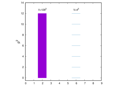
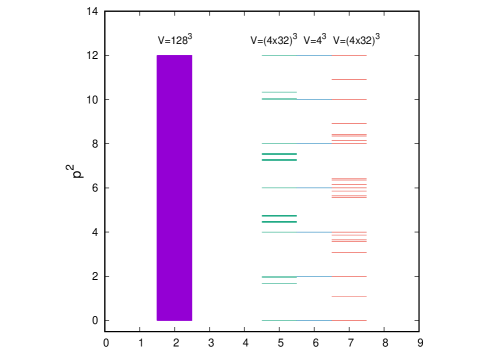
Figure 1: In plot a), on the left, we show the original momenta for the lattices $V=128^{3}$ (left column) and $V=4^{3}$ (right column). The same momenta are reported in plot b), on the right, together with the allowed momenta, obtained by considering two different configurations for the lattice setup $V=(4\times 32)^{3}$, i.e. with $N=4$ and $m=32$. All simulations have been done using the SU(2) gauge group at $\beta=3.0$.

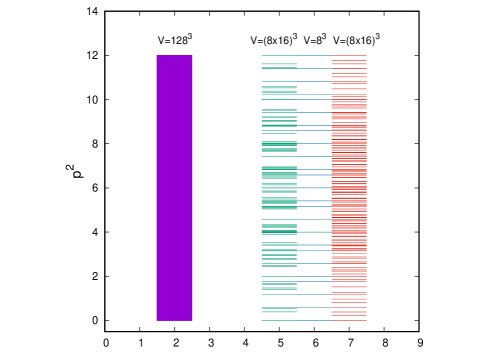
Figure 2: In plot a), on the left, we show the original momenta for the lattices $V=128^{3}$ (left column) and $V=8^{3}$ (right column). The same momenta are reported in plot b), on the right, together with the allowed momenta, obtained by considering two different configurations for the lattice setup $V=(8\times 16)^{3}$, i.e. with $N=8$ and $m=16$. All simulations have been done using the SU(2) gauge group at $\beta=3.0$.

We also stress that the explanation presented in section 5.4 about the suppression of $D(\vec{0}\mkern 2.0mu)$, in the limit $m\to\infty$, is essentially in agreement with the intuitive argument presented in ref. Cucchieri:2016qyc . To see this, using eqs. (239) and (222), we can write

$$\;{\widetilde{A}}^{jj}_{\mu}(l;\vec{0}\mkern 2.0mu)=\sum_{\vec{x}\in\Lambda_{x}}\!\Biggl{\{}\frac{1}{2i}\Bigl{[}U^{jj}_{\mu}(h;\vec{x}\mkern 1.0mu)e^{-\frac{2\pi in_{\mu}^{j}}{mN}}\!-\,e^{\frac{2\pi in_{\mu}^{j}}{mN}}{U^{jj}_{\mu}(h;\vec{x}\mkern 1.0mu)}^{*}\Bigr{]}-\frac{1}{N_{c}}\!\sum_{l=1}^{N_{c}}\Im\!\left[U^{ll}_{\mu}(h;\vec{x}\mkern 1.0mu)\,e^{\frac{-2\pi in_{\mu}^{l}}{mN}}\!\right]\Biggr{\}}\,,\;\;$$ (246)

i.e., we are evaluating the diagonal $jj$ coefficients of the matrix, see eq. (98),

$$\,\frac{1}{2i}\,\Bigl{[}\,Z_{\mu}(h)\,e^{-i\frac{\Theta_{\mu}}{N}}\,-\,e^{i\frac{\Theta_{\mu}}{N}}\,Z_{\mu}^{\dagger}(h)\,\Bigr{]}\,-\,1\!\!\!\bot\,\frac{\Im\operatorname{Tr}}{N_{c}}\!\left[\,Z_{\mu}(h)e^{-i\frac{\Theta_{\mu}}{N}}\,\right]$$ (247)

$$= \,\frac{1}{2i}\,\Bigl{[}\,Z_{\mu}(h)\,v^{\dagger}\,T_{\mu}\,v-\,v^{\dagger}\,T_{\mu}^{\dagger}\,v\,Z_{\mu}^{\dagger}(h)\,\Bigr{]}\,-\,1\!\!\!\bot\,\frac{\Im\operatorname{Tr}}{N_{c}}\!\left[\,Z_{\mu}(h)\,v^{\dagger}\,T_{\mu}\,v\,\right]\,,$$

where $T_{\mu}$ is a shorthand notation for the diagonal matrices $T_{\mu}(mN;\{n_{\mu}^{j}\})$, see eqs. (131) and (132). Hence, with $w_{j}=v^{\dagger}\,\hat{e}_{j}$, we end up with the expression

$${\widetilde{A}}^{jj}_{\mu}(l;\vec{0}\mkern 2.0mu)\, = \,\hat{e}_{j}^{\dagger}\;\frac{v\,Z_{\mu}(h)\,v^{\dagger}\,T_{\mu}\,-\,T_{\mu}^{\dagger}\,v\,Z_{\mu}^{\dagger}(h)v^{\dagger}}{2\,i}\,\hat{e}_{j}\,-\,\frac{\Im\operatorname{Tr}}{N_{c}}\!\left[\,Z_{\mu}(h)\,v^{\dagger}\,T_{\mu}\,v\,\right]$$ (248)

$$= \,\hat{e}_{j}^{\dagger}\;\frac{V_{\mu}\,-\,V_{\mu}^{\dagger}}{2\,i}\,\hat{e}_{j}\,-\,\frac{\Im\operatorname{Tr}}{N_{c}}\,V_{\mu}\;,$$

where we defined $V_{\mu}\equiv v\,Z_{\mu}(h)\,v^{\dagger}\,T_{\mu}$. At the same time, in order to impose the gauge-fixing condition, we need to maximize the quantity, see eq. (97),

$$\Re\,\operatorname{Tr}\,\sum_{\mu=1}^{d}\,Z_{\mu}(h)\,e^{-i\frac{\Theta_{\mu}}{N}}\,=\,\Re\,\operatorname{Tr}\,\sum_{\mu=1}^{d}\,Z_{\mu}(h)\,v^{\dagger}\,T_{\mu}\,v\,=\,\Re\,\operatorname{Tr}\,\sum_{\mu=1}^{d}\,V_{\mu}\,.$$ (249)

Intuitively, this maximization can be easily achieved if one finds a global rotation $v$ such that the (rotated) zero modes $v\,Z_{\mu}(h)\,v^{\dagger}$ become close to diagonal matrices. Then, given that in the limit $m\to\infty$ the discretized parameters $n_{\mu}^{j}/mN$ become continuous, one should be able to use the diagonal matrices $T_{\mu}=T_{\mu}(mN;\{n_{\mu}^{j}\})$ — whose elements are ${T_{\mu}}^{jj}=\exp{(-2\pi in_{\mu}^{j}/m\,N})$ — to bring the matrices $V_{\mu}$ as close as possible to real diagonal matrices. As a consequence, both terms in eq. (248) should be close to zero, implying ${\widetilde{A}}^{jj}_{\mu}(l;\vec{0}\mkern 2.0mu)\approx 0$ and $D(\vec{0}\mkern 2.0mu)\approx 0$, see eqs. (238).

As we noted in section 4, gauge-fixed link configurations within each replicated lattice $\Lambda_{x}^{(\vec{y}\mkern 1.0mu)}$ are rotated, transformed by global group elements defined by the cell index ${\vec{y}}$, see eq. (119). The same applies to the gauge-fixed gauge-field configurations $\{A_{\mu}(l;\vec{x}\mkern 1.0mu)\}$, see eq. (157). It is then natural to consider, on each replicated lattice $\Lambda_{x}^{(\vec{y}\mkern 1.0mu)}$, the average color magnetization $\vec{M}_{\mu}(\vec{y})$ with (color) components

$$M_{\mu}^{b}(\vec{y})\,=\,\frac{1}{V}\,\sum_{\vec{x}\in\Lambda_{x}}\,A_{\mu}^{b}(g;\vec{x}+\vec{y}N)\;,$$ (251)

which is related to the gluon propagator at zero momentum since, see eq. (216),

$${\widetilde{A}}_{\mu}^{b}(g;\vec{0}^{\mkern 2.0mu\prime}\mkern 1.0mu)\,=V\,\sum_{\vec{y}\in\Lambda_{y}}\,M_{\mu}^{b}(\vec{y})\;,$$ (252)

so that eq. (232) implies by the expression

$$D(\vec{0}^{\mkern 2.0mu\prime}\mkern 1.0mu)\,=\,\frac{\operatorname{Tr}}{2\,m^{d}\,{\cal N}}\,\sum_{\mu=1}^{d}\,\Bigl{<}\left[\,{\widetilde{A}}_{\mu}(g;\vec{0}^{\mkern 2.0mu\prime}\mkern 1.0mu)\,\right]^{2}\Bigr{>}\,=\,\frac{V^{2}}{m^{d}\,{\cal N}}\,\sum_{\mu=1}^{d}\,\sum_{b=1}^{N_{c}^{2}-1}\,\Biggl{<}\biggl{[}\;\sum_{\vec{y}\mkern 1.0mu\in\Lambda_{y}}M_{\mu}^{b}(\vec{y}\mkern 1.0mu)\;\biggr{]}^{2}\Biggr{>}\,,$$ (253)

where ${\cal N}\equiv d(N_{c}^{2}-1)V$ has been defined in section 2.2. We show in Figs. 3 and 4 the vectors $\vec{M}_{3}(\vec{y})$ of the color magnetization, obtained in a simulation for the $SU(2)$ case and with lattice volume $V=(64\times 4)^{3}$ at $\beta=3.0$. The vector components stand for the different values of the color index, i.e. $M^{b}_{3}(\vec{y}\mkern 1.0mu)$, for $b=1,2,3$. One can clearly see the effect of the Bloch waves. In particular, the average magnetization may appear “smooth” along a certain direction when moving from one cell to the next, but a suitably chosen projection reveals the modulated behavior, as expected. For example, in Fig. 4, $M_{\mu}^{3}(\vec{y})$ does not change when crossing a boundary, while $M_{\mu}^{1}(\vec{y})$ and $M_{\mu}^{2}(\vec{y})$ are rotated (see Fig. 5). Thus, each cell $\Lambda_{x}^{(\vec{y}\mkern 1.0mu)}$ may be seen as a domain, and the domain walls are characterized by the cell boundaries.

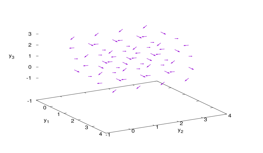
Figure 3: Average color “magnetization” $\vec{M}_{3}(\vec{y})$ on each replicated lattice $\Lambda_{x}^{(\vec{y}\mkern 1.0mu)}$ for the pure-$SU(2)$ case and lattice volume $V=(64\times 4)^{3}$, at $\beta=3.0$. In this case the index lattice $\Lambda_{y}$ is a $4^{3}$ lattice and $\vec{y}\mkern 1.0mu$ has components $y_{\mu}=0,1,2,3$ with $\mu=1,2,3$. Also note that the color components $M_{3}^{b}(\vec{y})$ (with $b=1,2$ and $3$) are represented along the corresponding spatial directions $\mu=1,2,3$.

Finally, we present our conclusions. Our main finding is that the gluon propagator $D(\vec{k}^{\mkern 1.0mu\prime}\mkern 1.0mu)$ is nonzero only for the allowed momenta and, in these cases, its value comes from some of the coefficients ${\widetilde{A}}^{ij}_{\mu}(g;\vec{k}^{\mkern 1.0mu\prime}\mkern 1.0mu)$, with all the other coefficients being equal to zero. Hence, we now completely understand the math behind the use of Bloch waves in minimal Landau gauge and we can perform the whole simulation (thermalization, gauge fixing and evaluation of the gluon propagator) in the small “unit cell” $\Lambda_{x}$. This should permit us to produce large ensembles of data for the infrared gluon propagator, even when we consider small unit cells and large values of $m$. We hope this can give us some hints about the role of the $\{U_{\mu}(h,\Theta;\vec{x})\}$ “domains” and of the “magnetization” described above. In particular, we want to find the minimum value of the lattice size $N$ of $\Lambda_{x}$ for which the momentum-space gluon propagator $D(\vec{k}^{\mkern 1.0mu\prime}\mkern 1.0mu)$, evaluated on $\Lambda_{z}$ using the Bloch setup with a factor $m$, is still in agreement with numerical data obtained by working directly on a lattice of size $mN$. More in general, we want to check the dependence of $D(\vec{k}^{\mkern 1.0mu\prime}\mkern 1.0mu)$ on $N$, while keeping the product $mN$ fixed. Clearly, since we know that finite-size effects in the gluon propagator are relevant only in the infrared regime, it is essential to consider all allowed momenta in these numerical simulations. Indeed, the momenta given by the discretization on the original (small) lattice $\Lambda_{x}$ are insufficient to adequately probe the infrared limit when $N$ is small. We also plan to extend this analysis to the ghost propagator.

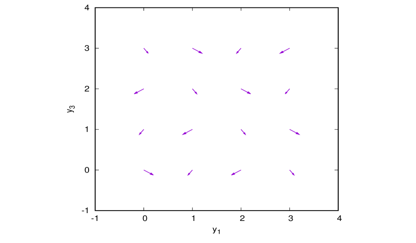
Figure 4: Average color “magnetization” $\vec{M}_{3}(\vec{y})$ on each replicated lattice $\Lambda_{x}^{(\vec{y}\mkern 1.0mu)}$ for the pure-$SU(2)$ case and lattice volume $V=(64\times 4)^{3}$, at $\beta=3.0$. In this case the index lattice $\Lambda_{y}$ is a $4^{3}$ lattice and $\vec{y}\mkern 1.0mu$ has components $y_{\mu}=0,1,2,3$ with $\mu=1,2,3$. Also note that the color components $M_{3}^{b}(\vec{y})$ (with $b=1,2$ and $3$) are represented along the corresponding spatial directions $\mu=1,2,3$. Here we show the data presented in Fig. 3 with coordinate $y_{2}=0$, projected on the $y_{1}\!-\!y_{3}$ plane. Consequently, we are also showing only the $b=1,3$ color components.

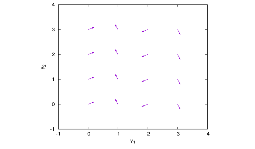
Figure 5: Average color “magnetization” $\vec{M}_{3}(\vec{y})$ on each replicated lattice $\Lambda_{x}^{(\vec{y}\mkern 1.0mu)}$ for the pure-$SU(2)$ case and lattice volume $V=(64\times 4)^{3}$, at $\beta=3.0$. In this case the index lattice $\Lambda_{y}$ is a $4^{3}$ lattice and $\vec{y}\mkern 1.0mu$ has components $y_{\mu}=0,1,2,3$ with $\mu=1,2,3$. Also note that the color components $M_{3}^{b}(\vec{y})$ (with $b=1,2$ and $3$) are represented along the corresponding spatial directions $\mu=1,2,3$. Here we show the data presented in Fig. 3 with coordinate $y_{3}=0$, projected on the $y_{1}\!-\!y_{2}$. Consequently, we are also showing only the $b=1,2$ color components.

Appendix A Cartan sub-algebra

In this appendix we discuss properties related to the matrices $\Theta_{\mu}$, introduced in section 3.2, see eq. (94). Recall that these matrices belong to the Cartan sub-algebra of $su(N_{c})$ and must satisfy the periodicity condition (100), which implies that their eigenvalues be given by $2\pi n_{\mu}/m$, where $n_{\mu}$ is an integer. We start by describing a general parametrization for the $N_{c}-1$ generators of the Cartan sub-algebra in the SU($N_{c}$) case Cornwell ; vanEgmond:2021wlt ; Zuber , and then comment on possible advantages of other bases. We also compare our setup with that considered in ref. Zwanziger:1993dh . As can be seen in section 5, and in particular in subsections 5.3 and 5.4, some of these properties are central to obtain an analytic expression for the gluon propagator using the gauge-fixed configuration on the extended lattice $\Lambda_{z}$.

We recall that we have chosen the $N_{c}^{2}-1$ traceless generators $t^{b}$ of the $su(N_{c})$ Lie algebra to be Hermitian. Since the Cartan generators $\{t_{\scriptscriptstyle C}\}$ are mutually commuting, i.e. $[t^{a}_{\scriptscriptstyle C},t^{b}_{\scriptscriptstyle C}]=0$ (for $a,b=1,\ldots,N_{c}-1$), they can be simultaneously diagonalized. For example, in the SU($N_{c}$) case, we can consider as diagonal Cartan generators (in the fundamental representation) the $N_{c}-1$ linearly independent, $N_{c}\times N_{c}$ Hermitian and traceless matrices $H^{i}$ ($i=1,\ldots,N_{c}-1$) defined by Zuber

$$H^{i}_{jk}\,=\,\xi^{i}\,\delta^{jk}\,\left[\delta^{ij}-\delta^{(i+1)j}\right]\,,$$ (254)

with $\xi^{i}$ real and $j,k=1,\ldots,N_{c}$. Note that, beside being diagonal, the matrix $H^{i}$ only has nonzero elements in rows/columns $i$ and $i+1$ and these two elements have opposite signs, enforcing the tracelessness condition. In particular, for $N_{c}=2$, the matrix $H^{1}$ is given by $\xi^{1}$ times the third Pauli matrix $\sigma_{3}$. For the SU($3$) case, after setting $\xi^{1}=\xi^{2}=1$, we have

$$H^{1}\,=\,\begin{pmatrix}1&0&0\\ 0&-1&0\\ 0&0&0\end{pmatrix}\qquad\mbox{and}\qquad H^{2}\,=\,\begin{pmatrix}0&0&0\\ 0&1&0\\ 0&0&-1\end{pmatrix}\;.$$ (255)

Since they are diagonal, the above generators $H^{i}$ have — as common eigenvectors — the unit vectors $\hat{e}_{j}$ [whose components are given by $(\hat{e}_{j})_{k}=\delta^{jk}$], with eigenvalues $\lambda^{i}_{j}=\xi^{i}\left[\delta^{ij}-\delta^{(i+1)j}\right]$, where again $j=1,\ldots,N_{c}$.

More in general, since the matrices $H^{i}$ are diagonal, we may define the Cartan generators by any combination

$$D^{i}\,=\,\sum_{l=1}^{N_{c}-1}\,R^{il}\,H^{l}\;,$$ (256)

where $R$ is an invertible $(N_{c}\!-\!1)\times(N_{c}\!-\!1)$ matrix. For example, in the SU($3$) case, with the Gell-Mann choice for the generators of the group algebra, the Cartan sub-algebra is spanned by the matrices $D^{1}=H^{1}$ and $D^{2}=(H^{1}+2H^{2})/\sqrt{3}$ — usually denoted by $\lambda_{3}$ and $\lambda_{8}$ — instead of $H^{1}$ and $H^{2}$ given in eq. (255). This corresponds to changing the basis with the matrix

$$R\,=\,\begin{pmatrix}1&0\\ \frac{1}{\sqrt{3}}&\frac{2}{\sqrt{3}}\end{pmatrix}\;.$$ (257)

In order to generalize the above bases containing Pauli and Gell-Mann matrices to the SU($N_{c})$ case (see, e.g., appendix A1 in ref. Smit ), we may consider the matrices

$$D^{i}\,=\,\sqrt{\frac{2}{i(i+1)}}\,\left[\,\sum_{l=1}^{i}\,l\,H^{l}\,\right]\;,$$ (259)

with $i=1,\ldots,N_{c}\!-\!1$. Note that, just as $H^{i}$, the matrices $D^{i}$ are diagonal. Their eigenvectors are also $\hat{e}_{j}$, but with eigenvalues

$$\alpha^{i}_{j}\,=\,\sum_{l=1}^{N_{c}-1}\,R^{il}\,\lambda^{l}_{j}\,=\,R^{ij}\,\xi^{j}-R^{i(j-1)}\,\xi^{j-1}\;.$$ (260)

Also, recall that, while $j$ takes values from $1$ to $N_{c}$, the indices of the matrix $R^{il}$ and of the constants $\xi^{i}$ only go from $1$ to $N_{c}\!-\!1$. Thus, for $j=1$ we have $\alpha^{i}_{1}=R^{i1}\,\xi^{1}$ and for $j=N_{c}$ we find $\alpha^{i}_{N_{c}}=-R^{i(N_{c}-1)}\,\xi^{N_{c}-1}$.

Finally, it is rather evident Cornwell ; Zuber that, if $H_{\scriptscriptstyle C}$ is a Cartan sub-algebra and $v$ is any element of the Lie group, the conjugate $v^{-1}\,H_{\scriptscriptstyle C}\,v$ is another Cartan sub-algebra. Thus, for the SU($N_{c})$ group we can consider as matrices $t_{\scriptscriptstyle C}^{b}$ the set $\{v^{\dagger}\,D^{b}\,v\}$, with common eigenvectors $\{w_{j}=v^{\dagger}\,\hat{e}_{j}\;\mbox{for}\;j=1,\ldots,N_{c}\}$ — which are orthonormal, since $w_{j}^{\dagger}\,w_{k}=\hat{e}_{j}^{\dagger}\,\hat{e}_{k}\,=\,\delta^{jk}$ — and the eigenvalues $\alpha^{b}_{j}$ given above, where we switched back to the usual index $b$ for the color degrees of freedom. This illustrates the expansion in eq. (94).

A.1 Comparison with reference Zwanziger:1993dh

We note that ref. Zwanziger:1993dh defines the $\Theta_{\mu}$ matrices, belonging to a generic Cartan sub-algebra, as an expansion in terms of the generators $t^{b}$ of the SU($N_{c}$) algebra, i.e.,

$$\Theta_{\mu}\,=\,\sum_{b=1}^{N_{c}^{2}-1}\,\theta_{\mu}^{b}\,t^{b}\,,$$ (261)

with real parameters $\theta_{\mu}^{b}$ ($\mu=1,\ldots,d$), subject to the condition

$$\left[\,\Theta_{\mu},\,\Theta_{\nu}\,\right]\,=\,\sum_{b,c=1}^{N_{c}^{2}-1}\,\,\theta_{\mu}^{b}\,\theta_{\nu}^{c}\,\left[\,t^{b},\,t^{c}\,\right]\,=\,2\,i\,\sum_{a,b,c=1}^{N_{c}^{2}-1}\,\,f^{abc}\,\theta_{\mu}^{b}\,\theta_{\nu}^{c}\;t^{a}\,\,=\,0\;,$$ (262)

where we denote by $f^{abc}$ the structure constants of the $su(N_{c})$ Lie algebra. Now, since the matrices $t^{a}$ are linearly independent, the above equality implies that

$$\sum_{b,c=1}^{N_{c}^{2}-1}\,f^{abc}\,\theta_{\mu}^{b}\,\theta_{\nu}^{c}\,=\,0\;,$$ (263)

for any $a=1,\ldots,N_{c}^{2}-1$.

In the SU($2$) case, for example, for which the Cartan sub-algebra is one-dimensional and the structure constants $f^{abc}$ are given by the completely anti-symmetric tensor $\epsilon^{abc}$, we find that the above condition is equivalent to saying that the three-dimensional vectors $\vec{\theta}_{\mu}$ and $\vec{\theta}_{\nu}$ must be parallel for any $\mu,\nu$. This can be easily achieved Zwanziger:1993dh with

$$\Theta_{\mu}\,=\,r_{\mu}\,\sum_{b=1}^{3}\,\,q^{b}\,t^{b}\;,$$ (264)

where $r_{\mu}$ and $q^{b}$ are real parameters. As a matter of fact, by factoring $\,\theta^{b}_{\mu}=\,r_{\mu}\,q^{b}$, i.e. by imposing that the vectors $\vec{\theta}_{\mu}$ are all proportional to the vector $\vec{q}$, it is evident that eq. (263) is satisfied, since $\sum_{b,c=1}^{3}f^{abc}q^{b}q^{c}=0$. Note that matrices $\Theta_{\mu}$ defined in this way are not necessarily diagonal. On the other hand, they are mutually commuting since they are proportional to the same matrix $\sum_{b=1}^{3}\,\,q^{b}\,t^{b}$. One can also write

$$\Theta_{\mu}\,=\,r_{\mu}\,v^{\dagger}\,\sigma_{3}\,v\;,$$ (265)

where $v\in$ SU(2) and $\sigma_{3}$ is the third Pauli matrix, which is diagonal. Indeed, eqs. (264) and (265) are completely equivalent. Hence, the above parametrization (265) is clearly in agreement with the previously discussed setup and we can say that the expansion used in ref. Zwanziger:1993dh corresponds to a transformation $v^{-1}\,H_{\scriptscriptstyle C}\,v$ of the Cartan sub-algebra given by $\sigma_{3}$. Note that, using eq. (265), the matrices $\Theta_{\mu}$ trivially have eigenvectors

$$v^{\dagger}\begin{pmatrix}1\\ 0\end{pmatrix}$$ (267)

and

$$v^{\dagger}\begin{pmatrix}0\\ 1\end{pmatrix}$$ (268)

with eigenvalues $\pm\,r_{\mu}$.

In like manner, in the SU(3) case, which has rank two, we can write Zwanziger:1993dh

$$\Theta_{\mu}\,=\,r_{\mu,3}\,\sum_{b=1}^{8}\,\,q^{b}_{3}\,t^{b}\,+\,r_{\mu,8}\,\sum_{b=1}^{8}\,\,q^{b}_{8}\,t^{b}$$ (269)

with real parameters $r_{\mu,3},\,r_{\mu,8},\,q^{b}_{3}$ and $q^{b}_{8}$, i.e. we now factored $\,\theta^{b}_{\mu}=r_{\mu,3}\,q^{b}_{3}+r_{\mu,8}\,q^{b}_{8}$. This yields, see eq. (263),

$$\sum_{b,c=1}^{8}\,f^{abc}\,q^{b}_{3}\,q^{c}_{8}\,\left(\,r_{\mu,3}\,r_{\nu,8}\,-\,r_{\mu,8}\,r_{\nu,3}\,\right)\,=\,0\;,$$ (270)

where we used the (obvious) relation $f^{abc}=-f^{acb}$. Clearly, since the above expression must be valid for any values of the parameters $r_{\mu,3}$ and $r_{\mu,8}$, we must select two commuting matrices

$$\widetilde{\lambda}_{3}\,=\,\sum_{b=1}^{8}\,\,q^{b}_{3}\,t^{b}\qquad\qquad\mbox{and}\qquad\qquad\widetilde{\lambda}_{8}\,=\,\sum_{c=1}^{8}\,\,q^{c}_{8}\,t^{c}$$ (271)

to parametrize the expansion of $\Theta_{\mu}$, so that

$$\frac{1}{2}\,\operatorname{Tr}\,\left\{\,t^{a}\,\left[\,\widetilde{\lambda}_{3},\,\widetilde{\lambda}_{8}\,\right]\right\}\,=\,\sum_{b,c=1}^{8}\,f^{abc}\,q^{b}_{3}\,q^{c}_{8}\,=\,0\;.$$ (272)

Then, we recover again our definition for $\Theta_{\mu}$ — in terms of diagonal matrices and the transformation $v^{-1}\,H_{\scriptscriptstyle C}\,v$ — if we consider

$$\Theta_{\mu}\,=\,r_{\mu,3}\,\widetilde{\lambda}_{3}\,+\,r_{\mu,8}\,\widetilde{\lambda}_{8}\,=\,\,v^{\dagger}\,\left(\,r_{\mu,3}\,\lambda_{3}\,+\,r_{\mu,8}\,\lambda_{8}\,\right)\,v\;,$$ (273)

where $\lambda_{3}$ and $\lambda_{8}$ are the two diagonal Gell-Mann matrices and $v\in$ SU(3).

A.2 New basis for the Lie algebra

As already noted above, the matrices $\Theta_{\mu}$ — which belong to the Cartan sub-algebra and are written in terms of the basis $\,t_{\scriptscriptstyle C}^{b}=v^{\dagger}D^{b}v$ — have eigenvectors $w_{j}=v^{\dagger}\,\hat{e}_{j}$ (for $j=1,\ldots,N_{c}$), with eigenvalues given by

$$\Theta_{\mu}\,w_{j}\,=\,\left[\,\sum_{b=1}^{N_{c}-1}\,\theta_{\mu}^{b}\,\alpha^{b}_{j}\,\right]\,w_{j}\,\equiv\,\beta_{\mu}^{j}\,w_{j}\,=\,\frac{2\pi\,n_{\mu}^{j}}{m}\,w_{j}\;,$$ (274)

where the parameters $\theta_{\mu}^{b}$ refer to the expansion in eq. (94), $\alpha^{b}_{j}$ is defined in eq. (260) and, in the last step, we imposed the constraint (100), i.e. that $n_{\mu}^{j}$ be integers.

Then, it is natural to consider a new basis for $\Theta_{\mu}$, with matrices defined as an outer product of these eigenvectors, i.e.,

$${\bf W}^{ij}\equiv w_{i}\,w_{j}^{\dagger}\,=\,v^{\dagger}\,\hat{e}_{i}\,\hat{e}_{j}^{\dagger}\,v\,\equiv\,v^{\dagger}\,{\bf M}^{ij}\,v\,,$$ (275)

where the matrix element $\,lm\,$ of ${\bf W}^{ij}$ is given by $(w_{i})_{l}\,(w_{j}^{\dagger})_{m}$ (for $l,m=1,\ldots,N_{c}$). Similarly, we have also defined the $N_{c}\times N_{c}$ matrix ${\bf M}^{ij}=\hat{e}_{i}\,\hat{e}_{j}^{\dagger}$, whose elements are simply $({\bf M}^{ij})_{lm}=\delta^{il}\delta^{jm}$. In this way, considering $\,\Theta_{\mu}=\sum_{i,j}c_{\mu}^{ij}\,{\bf W}^{ij}$, we can left multiply eq. (274) by $w_{i}^{\dagger}$ to obtain the expansion parameters

$$c_{\mu}^{ij}\,=\,w_{i}^{\dagger}\,\Theta_{\mu}\,w_{j}\,=\,\beta_{\mu}^{i}\,\delta^{ij}\,=\,\frac{2\pi\,n_{\mu}^{i}}{m}\,\delta^{ij}$$ (276)

in the ${\bf W}^{ij}$ basis. As expected, they are nonzero only for $i=j$, since the eigenvectors $w_{i}$ form an orthonormal set. Thus, we can write

$$\Theta_{\mu}\,=\,\sum_{j=1}^{N_{c}}\beta_{\mu}^{j}\;{\bf W}^{jj}\,=\,\sum_{j=1}^{N_{c}}\,\frac{2\pi\,n_{\mu}^{j}}{m}\,v^{\dagger}\,{\bf M}^{jj}\,v$$ (277)

and

$$\exp{\left(i\,\frac{\Theta_{\mu}}{N}\right)}\,=\,v^{\dagger}\,\exp{\left(\sum_{j=1}^{N_{c}}\,\frac{2\pi i\,n_{\mu}^{j}}{mN}\,{\bf M}^{jj}\,\right)}\,v\;,$$ (278)

which are important results for our analysis in sections 3.3 and 4. Of course, when $v=1\!\!\!\bot$ — or, equivalently, when considering the basis ${\bf M}^{ij}$ — the matrices in eqs. (277) and (278) are diagonal.

Let us stress that the matrices ${\bf W}^{ij}$ trivially satisfy the trace condition

$$\operatorname{Tr}\left({\bf W}^{ij}\right)\,=\,\operatorname{Tr}\left(w_{i}\,w_{j}^{\dagger}\right)\,=\,w_{j}^{\dagger}\,w_{i}\,=\,\delta^{ij}$$ (279)

and the orthonormality relations

$$\operatorname{Tr}\left({\bf W}^{ij}\,{{\bf W}^{lm}}^{\dagger}\,\right)=\,\operatorname{Tr}\left({\bf W}^{ij}\,{\bf W}^{ml}\right)=\operatorname{Tr}\left(w_{i}\,w_{j}^{\dagger}\,w_{m}\,w_{l}^{\dagger}\,\right)\,=\,\delta^{jm}\,\operatorname{Tr}\left(w_{i}\,w_{l}^{\dagger}\,\right)=\,\delta^{jm}\,\delta^{il}\;,$$ (280)

where we used ${{\bf W}^{lm}}^{\dagger}={\bf W}^{ml}$, the orthonormality of the $w$’s and (279). Hence, the $N_{c}^{2}$ matrices ${\bf W}^{ij}$ are indeed a basis for any $N_{c}\times N_{c}$ matrix, which is — as seen in section 5 — the most natural one to consider when analyzing the impact of the index lattice on the evaluation of the gluon propagator. On the other hand, elements of the (real) SU($N_{c}$) Lie group — as well as of the corresponding $su(N_{c})$ Lie algebra — are written in terms of $N_{c}^{2}\!-\!1$ real independent parameters. Therefore, when using this basis, the $N_{c}^{2}$ coefficients entering the linear combination of the ${\bf W}^{ij}$ matrices are not all independent. As a matter of fact, a generic matrix

$$A\,=\,\sum_{i,j=1}^{N_{c}}A^{\mkern 1.0muij}\,{\bf W}^{ij}\,,$$ (282)

where the coefficients $A^{ij}$ are given, see eq. (276), by

$$A^{ij}\,=\,w_{i}^{\dagger}\,A\,w_{j}\;,$$ (283)

is (in general) not traceless, due to eq. (279). Thus, for the $su(N_{c})$ Lie algebra we have to enforce the constraint

$$0\,=\,\operatorname{Tr}A\,=\,\sum_{j=1}^{N_{c}}\,A^{\mkern 1.0mujj}\;,$$ (284)

yielding the relation, see eq. (277),

$$0\,=\,\sum_{j=1}^{N_{c}}\,\beta_{\mu}^{j}\,=\,\frac{2\pi}{m}\,\sum_{j=1}^{N_{c}}\,n_{\mu}^{j}$$ (285)

for the $\Theta_{\mu}$ matrices. Of course, this condition is automatically satisfied if the $\beta_{\mu}^{j}$ eigenvalues are given, see eqs. (274) and (260), by

$$\beta_{\mu}^{j}\,=\,\sum_{b=1}^{N_{c}-1}\,\theta_{\mu}^{b}\,\alpha^{b}_{j}\,=\,\sum_{b=1}^{N_{c}-1}\,\theta_{\mu}^{b}\,\left[\,R^{bj}\,\xi^{j}-R^{b(j-1)}\,\xi^{j-1}\,\right]\;,$$ (286)

which implies

$$\sum_{j=1}^{N_{c}}\,\beta_{\mu}^{j}\,=\,\sum_{j=1}^{N_{c}-1}\,\sum_{b=1}^{N_{c}-1}\,\theta_{\mu}^{b}\,R^{bj}\,\xi^{j}\,-\,\sum_{j=2}^{N_{c}}\,\sum_{b=1}^{N_{c}-1}\,\theta_{\mu}^{b}\,R^{b(j-1)}\,\xi^{j-1}\,=\,0\;.$$ (287)

Indeed, when written in terms of the coefficients $\theta_{\mu}^{b}$, see eq. (94), the matrices $\Theta_{\mu}$ depend on $d\,(N_{c}\!-\!1)$ free parameters; on the other hand, when they are written using the $n_{\mu}^{j}$ coefficients, see eq. (277), we have $d\,N_{c}$ free parameters, subject to the $d$ constraints (285).

Beside being traceless, an element of the SU($N_{c})$ Lie algebra should also be (with our convention) Hermitian. Hence, if we impose $A^{\dagger}=A$ in eq. (282), we find

$$\left(A^{\mkern 1.0muij}\right)^{*}\,=\,A^{\mkern 1.0muji}\;,$$ (288)

given that $\left({\bf W}^{ij}\right)^{\dagger}={\bf W}^{ji}$, see footnote 60. (Here, ^∗ denotes complex conjugation.) The last result, together with eq. (284), implies that the diagonal coefficients $A^{\mkern 1.0mujj}$ are real and that only $N_{c}\!-\!1$ of them are independent. At the same time, from eq. (288) we find that there are only $N_{c}\,(N_{c}\!-\!1)/2$ independent complex off-diagonal elements, yielding a total of $(N_{c}-1)+(N_{c}^{2}-N_{c})=N_{c}^{2}\!-\!1$ free real parameters (as expected). We stress that the coefficients $A^{\mkern 1.0muij}$ are not the matrix elements of $A$, which are given by the expression

$$A_{lm}\,=\,\sum_{i,j=1}^{N_{c}}\left({\bf W}^{ij}\right)_{lm}\;A^{\mkern 1.0muij}$$ (289)

with

$$\left({\bf W}^{ij}\right)_{lm}\,=\,\sum_{k,n=1}^{N_{c}}\left(v^{\dagger}\right)_{lk}\,\left({\bf M}^{ij}\right)_{kn}\,v_{nm}\,=\,\left(v^{\dagger}\right)_{li}\,v_{jm}\,=\,v_{il}^{*}\,v_{jm}\;,$$ (290)

so that one has (as always for a Hermitian matrix)

$$A_{lm}^{*}\, = \,\sum_{i,j=1}^{N_{c}}\,\left({\bf W}^{ij}\right)_{lm}^{*}\,\left(A^{\mkern 1.0muij}\right)^{*}\,=\,\sum_{i,j=1}^{N_{c}}\,\left[\,v_{il}^{*}\,v_{jm}\,\right]^{*}\,\left(A^{\mkern 1.0muij}\right)^{*}$$ (291)

$$= \,\sum_{i,j=1}^{N_{c}}\,v_{jm}^{*}\,v_{il}\,A^{\mkern 1.0muji}\,=\,\sum_{j,i=1}^{N_{c}}\,\left({\bf W}^{ji}\right)_{ml}\,A^{\mkern 1.0muji}\,=\,A_{ml}\;.$$

Finally, eq. (277) tells us that we can easily relate the Cartan sub-algebra, defined by the diagonal matrices in eqs. (254) and (256) above, with the matrices ${\bf M}^{jj}$ (or the matrices ${\bf W}^{jj}$). Indeed, given that $({\bf M}^{jj})_{lm}=\delta^{jl}\delta^{jm}$, we can write (for $i=1,\ldots,N_{c}\!-\!1$)

$$H^{i}\,=\,\xi^{i}\,\left[\,{\bf M}^{ii}\,-\,{\bf M}^{(i+1)(i+1)}\,\right]$$ (292)

so that

$$D^{i}\,=\,\sum_{j=1}^{N_{c}-1}R^{ij}\;\xi^{j}\,\left[\,{\bf M}^{jj}\,-\,{\bf M}^{(j+1)(j+1)}\,\right]$$ (293)

and

$$t_{\scriptscriptstyle C}^{i}\,=\,v^{\dagger}\,D^{i}\,v\,=\,\sum_{j=1}^{N_{c}-1}R^{ij}\,\xi^{j}\,\left[\,{\bf W}^{jj}\,-\,{\bf W}^{(j+1)(j+1)}\,\right]\;.$$ (294)

In particular, if we set $\xi^{j}=1$ in eq. (293) and we use the matrix $R$ defined in eq. (258), the matrices $D^{i}$ recover the generalized diagonal Gell-Matrices matrices, see eq. (259). It is interesting that, using the matrices ${\bf M}^{ij}$, we can easily define also the generalized nondiagonal Gell-Matrices matrices (see again appendix A1 in ref. Smit ):

$$t^{b}\,=\,{\bf M}^{ij}\,+\,{\bf M}^{ji}$$ (295)

and

$$t^{b}\,=\,-i\,\left(\,{\bf M}^{ij}\,-\,{\bf M}^{ji}\,\right)\;,$$ (296)

with $i,j=1,\ldots,N_{c}$ and $i<j$. Note that there are $N_{c}(N_{c}\!-\!1)/2$ symmetric matrices (295), $N_{c}(N_{c}\!-\!1)/2$ anti-symmetric matrices (296) and $N_{c}\!-\!1$ diagonal matrices $t_{\scriptscriptstyle C}^{i}=D^{i}$, for a total of $N_{c}^{2}-1$ (Hermitian and traceless) generators.

The above results imply that the (generic) matrix

$$M_{\scriptscriptstyle C}\,\equiv\,\sum_{i=1}^{N_{c}-1}\,m^{i}\,t_{\scriptscriptstyle C}^{i}\,=\,\sum_{i=1}^{N_{c}-1}\,m^{i}\,\sum_{j=1}^{N_{c}-1}R^{ij}\;\xi^{j}\,\left[\,{\bf W}^{jj}\,-\,{\bf W}^{(j+1)(j+1)}\,\right]\;,$$ (297)

which is in the Cartan sub-algebra, can also be written as

$$M_{\scriptscriptstyle C}\,=\,\sum_{j=1}^{N_{c}}\,a^{jj}\,{\bf W}^{jj}$$ (298)

with

$$a^{jj}\,=\,\sum_{i=1}^{N_{c}-1}\,m^{i}\,\left[\,R^{ij}\,\xi^{j}\,-\,R^{i(j-1)}\,\xi^{j-1}\right]\;.$$ (299)

However, one should stress that, on the l.h.s. of the above equation, the index $j$ takes (integer) values in the interval $[1,N_{c}]$, while, on the r.h.s., the indices $j$ and $j\!-\!1$ of $R$ and of $\xi$ are always restricted to the interval $[1,N_{c}-1]$. This implies the relations

$$a^{11}\, = \,\sum_{i=1}^{N_{c}-1}\,m^{i}\,R^{i1}\,\xi^{1}$$ (300)

$$a^{22}\, = \,\sum_{i=1}^{N_{c}-1}\,m^{i}\,\left(\,R^{i2}\,\xi^{2}\,-\,R^{i1}\,\xi^{1}\right)$$ (301)

$$a^{33}\, = \,\sum_{i=1}^{N_{c}-1}\,m^{i}\,\left(\,R^{i3}\,\xi^{3}\,-\,R^{i2}\,\xi^{2}\,\right)$$ (302)

$$\ldots$$ (303)

$$a^{\scriptscriptstyle{(N_{c}-1)(N_{c}-1)}}\, = \,\sum_{i=1}^{N_{c}-1}\,m^{i}\,\left[\,R^{i(N_{c}-1)}\,\xi^{N_{c}-1}\,-\,R^{i(N_{c}-2)}\,\xi^{N_{c}-2}\,\right]$$ (304)

$$a^{\scriptscriptstyle{N_{c}N_{c}}}\, = \,-\,\sum_{i=1}^{N_{c}-1}\,m^{i}\,R^{i(N_{c}-1)}\,\xi^{N_{c}-1}\;,$$ (305)

which trivially ensure the constraint (284).

References

• (1) A. Cucchieri and T. Mendes, Bloch Waves in Minimal Landau Gauge and the Infinite-Volume Limit of Lattice Gauge Theory, Phys. Rev. Lett. 118, no.19, 192002 (2017).
• (2) A. Cucchieri and T. Mendes, Numerical test of the Gribov-Zwanziger scenario in Landau gauge, PoS QCD-TNT09, 026 (2009).
• (3) A. Cucchieri, D. Dudal and N. Vandersickel, The No-Pole Condition in Landau gauge: Properties of the Gribov Ghost Form-Factor and a Constraint on the 2d Gluon Propagator, Phys. Rev. D85, 085025 (2012).
• (4) A. Cucchieri, D. Dudal, T. Mendes and N. Vandersickel, Modeling the Gluon Propagator in Landau Gauge: Lattice Estimates of Pole Masses and Dimension-Two Condensates, Phys. Rev. D85, 094513 (2012).
• (5) D. Zwanziger, Fundamental modular region, Boltzmann factor and area law in lattice gauge theory, Nucl. Phys. B412, 657 (1994).
• (6) L. Giusti, M. L. Paciello, C. Parrinello, S. Petrarca and B. Taglienti, Problems on lattice gauge fixing, Int. J. Mod. Phys. A16, 3487 (2001).
• (7) J. Greensite, The Confinement problem in lattice gauge theory, Prog. Part. Nucl. Phys. 51, 1 (2003).
• (8) V. N. Gribov, Quantization of Nonabelian Gauge Theories, Nucl. Phys. B139, 1 (1978).
• (9) D. Zwanziger, Nonperturbative Modification of the Faddeev-popov Formula and Banishment of the Naive Vacuum, Nucl. Phys. B209, 336 (1982).
• (10) G. Dell’Antonio and D. Zwanziger, Ellipsoidal Bound on the Gribov Horizon Contradicts the Perturbative Renormalization Group, Nucl. Phys. B326, 333 (1989).
• (11) N. Vandersickel and D. Zwanziger, The Gribov problem and QCD dynamics, Phys. Rept. 520, 175 (2012).
• (12) A. Cucchieri, T. Mendes and A. Mihara, Ghost condensation on the lattice, Phys. Rev. D72, 094505 (2005).
• (13) J. F. Cornwell, Group Theory in Physics: An Introduction, Academic Press, San Diego, U.S.A. (1997).
• (14) D. B. Leinweber et al. [UKQCD], Asymptotic scaling and infrared behavior of the gluon propagator, Phys. Rev. D60, 094507 (1999) [Erratum: Phys. Rev. D61, 079901 (2000)].
• (15) J. Smit, Introduction to Quantum Fields on a Lattice, Cambridge University Press, Cambridge, U.K. (2002).
• (16) C. Gattringer and C. B. Lang, Quantum chromodynamics on the lattice (An Introductory Presentation), Lect. Notes Phys. 788, Springer, Berlin, Germany (2010).
• (17) H. J. Rothe, Lattice Gauge Theories : An Introduction (Fourth Edition), World Sci. Lect. Notes Phys. 82, 1-606 (2012).
• (18) H. Suman and K. Schilling, A Comparative study of gauge fixing procedures on the connection machines CM2 and CM5, [arXiv:hep-lat/9306018 [hep-lat]].
• (19) A. Cucchieri and T. Mendes, Critical slowing down in SU(2) Landau gauge fixing algorithms, Nucl. Phys. B471, 263 (1996).
• (20) A. Cucchieri and T. Mendes, Study of critical slowing down in SU(2) Landau gauge fixing, Nucl. Phys. Proc. Suppl. 53, 811 (1997).
• (21) A. Cucchieri and T. Mendes, Critical slowing down in SU(2) Landau gauge fixing algorithms at $\beta=\infty$, Comput. Phys. Commun. 154, 1 (2003).
• (22) J. M. Leal, M. Cerqueira and T. Mendes, Efficiency Study of Overrelaxation and Stochastic Overrelaxation Algorithms for SU(3) Landau Gauge-Fixing, PoS LATTICE2021, 057 (2022).
• (23) D. Zwanziger, Vanishing of zero momentum lattice gluon propagator and color confinement, Nucl. Phys. B364, 127 (1991).
• (24) F. de Soto, Restoring rotational invariance for lattice QCD propagators, JHEP 10, 069 (2022).
• (25) A. Cucchieri, Gribov copies in the minimal Landau gauge: The Influence on gluon and ghost propagators, Nucl. Phys. B508, 353 (1997).
• (26) N. W. Ashcroft and N. D. Mermin, Solid State Physics, Harcourt Brace College Publishers, New York, U.S.A. (1976).
• (27) E. Marinari, C. Parrinello and R. Ricci, Evidence for the existence of Gribov copies in Landau gauge lattice QCD, Nucl. Phys. B362, 487 (1991).
• (28) J. M. Ziman, PRINCIPLES OF THE Theory of Solids, Cambridge University Press, Cambridge, UK, second edition (1972).
• (29) A. Gonzalez-Arroyo, Yang-Mills fields on the four-dimensional torus. Part 1.: Classical theory, in *Peniscola 1997, Advanced school on non-perturbative quantum field physics* 57-91, and [arXiv:hep-th/9807108 [hep-th]].
• (30) https://www.escherinhetpaleis.nl/story-of-escher/metamorphosis-i-ii-iii/ (last accessed 2nd of May 2025).
• (31) M. Grabenstein, Analysis and development of stochastic multigrid methods in lattice field theory, [arXiv:hep-lat/9401024 [hep-lat]].
• (32) C. A. Floudas, Nonlinear and Mixed-Integer Optimization. Fundamentals and Applications, Oxford University Press (Topics in Chemical Engineering), New York, NY, USA (1995).
• (33) M. Schaden and D. Zwanziger, Horizon condition holds pointwise on finite lattice with free boundary conditions, in *Paris 1994, Proceedings, Quantum infrared physics* 10-17, and [hep-th/9410019].
• (34) D. Zwanziger, Vanishing color magnetization in lattice Landau and Coulomb gauges, Phys. Lett. B257, 168-172 (1991).
• (35) A. Cucchieri and T. Mendes, Constraints on the IR behavior of the gluon propagator in Yang-Mills theories, Phys. Rev. Lett. 100, 241601 (2008).
• (36) D. M. van Egmond and U. Reinosa, SU($N$) Cartan-Weyl bases and color factors, [arXiv:2104.12139 [hep-th]].
• (37) J.-B. Zuber, Invariances in Physics and Group Theory, https://www.lpthe.jussieu.fr/ ˜zuber/Cours/InvariancesGroupTheory-2014.pdf (last accessed 2nd of May 2025).