Random Exclusion Codes: Quantum Advantages of Single-Shot Communication

Abstract

Identifying information tasks that offer advantages over their classical counterparts by exploiting quantum resources finds the usefulness of quantum information technologies. In this work, we introduce a two-party communication primitive, random exclusion code (REC), which is a single-shot prepare-and-measure protocol where a sender encodes a random message into a shorter sequence and a receiver attempts to exclude a randomly chosen letter in the original message. We present quantum advantages in RECs in two ways: probability and dimension. We show that RECs with quantum resources achieve higher success probabilities than classical strategies. We verify that the quantum resources required to describe detection events of RECs have a smaller dimension than classical ones. We also show that a guessing counterpart, random access codes (RACs), may not have a dimension advantage over classical resources. Our results elucidate various possibilities of achieving quantum advantages in two-party communication.

One of the key challenges in Quantum Information Theory is to address information tasks that demonstrate the distinct nature of quantum and classical resources. A gap appearing from the distinction, even if it is small, may be amplified toward practical applications, namely, quantum advantages in communication Winter (2013). It is hence of both fundamental and practical importance to identify a simplest information scenario, such as a point-to-point communication protocol, such that quantum advantages are present. The Holevo theorem is the first attempt along this line, considering a channel capacity with i.i.d. quantum states, but showing no quantum advantage Holevo (2011, 1998); Schumacher and Westmoreland (1997).

It is random access codes (RACs) that have verified the existence of quantum advantages in two-party communication Ambainis et al. (2009, 2024); Tavakoli et al. (2015); Carmeli et al. (2020). We emphasize that it is a single-shot scenario in which a single outcome is obtained from a detection event, from which a receiver learns about a message. Then, the guess is correct with some probability. The quantum advantage is demonstrated by the fact that the guessing probability in RACs is higher with quantum resources than classical strategies.

Although the connection is not direct, RACs are closely related to quantum state discrimination Helstrom (1969), see also Bae and Kwek (2015); Barnett and Croke (2009); Bergou (2007). Interestingly, quantum state anti-discrimination, which efficiently excludes a state from an ensemble, has been used as an effective tool to clarify the distinctions between quantum and classical resources in a single-shot experiment Caves et al. (2002); Pusey et al. (2012); Bandyopadhyay et al. (2014a); Heinosaari and Kerppo (2018). Quantum advantages can be obtained in terms of a success probability Uola et al. (2020); Ducuara et al. (2020), and a quantum-classical gap is also present in detection events. For instance, the Pusey-Barrett-Rudolph (PBR) theorem Pusey et al. (2012) rules out an impossible interpretation of quantum states by deriving a detection event that cannot happen with quantum resources.

Upon examining the fundamental tasks closely, it becomes clear that discrimination and exclusion are distinct in nature. Perfect discrimination of states achieves perfect exclusion by assigning an item from perfect guessing to another one. The converse does not generally hold. Thus, quantum state exclusion is operationally more general. Then, state exclusion may lead to even greater possibilities of quantum advantages.

As discussed above, efforts to distinguish quantum and classical resources in a single-shot scenario take one of the approaches. One is comparing the success probability for a single detection event; the probability with quantum resources is higher than that of classical ones, e.g., RACs. The other is to take into account the detection events. For instance, the PBR theorem signifies a detection event that is impossible to occur with quantum resources but is possible with independent ontic preparations Pusey et al. (2012); Harrigan and Spekkens (2010). Note that the Bell theorem is comparable to the latter in that it also rules out an ontic interpretation of quantum states; in contrast to the PBR result, two parties repeat a Bell experiment for estimating joint probabilities Bell (1964); Brunner et al. (2014). Then, it is worth mentioning that the quantum-classical gap from the Bell theorem has been developed as a practical tool for device-independent quantum information processing, such as randomness extraction Pironio et al. (2010), quantum key distribution Acín et al. (2007), state certification Šupić and Bowles (2020); Šupić et al. (2021), etc.

In this work, we present random exclusion codes (RECs) that leverage quantum state anti-discrimination to a communication primitive. Throughout, an $(n,m)$ REC of interest is a single-shot and prepare-and-measure protocol where a sender, Alice, encodes a random message of length $n$ using a set of $m$ letters into a $d$-dimensional system and transmits it. Bob, a receiver, realizes a decoding to exclude a chosen letter in the original message.

We show quantum advantages of RECs in two ways: one is the probability advantage for a single detection event, and the other is the dimension advantage for a collection of possible detection events. Firstly, a higher success probability in the exclusion task of a REC can be achieved with quantum resources than with classical ones. Secondly, quantum resources in a smaller Hilbert space achieve RECs that can be realized only in a larger classical dimension. Note that a classical dimension denotes the minimal number of distinguishable letters of an alphabet.

The importance of the results is twofold. On the one hand, we relate state exclusion, a fundamental tool for verifying distinctions between the elements of quantum and classical theories Caves et al. (2002); Bandyopadhyay et al. (2014b); Crickmore (2020); Pusey et al. (2012), to a communication primitive that may find practical applications. On the other hand, we demonstrate the quantum-classical gap within a single-shot framework by highlighting the differences between quantum and classical supports for detection events, see also Pusey et al. (2012). We also find that a RAC may not have a dimension advantage.

We begin with notations for an $(n,m)$ REC. A message of Alice is written by $a=a_{1}...a_{n}$ where each is chosen from a set of $m$ distinguishable letters, $a_{i}\in\{0,\cdots,m-1\}$. An encoding prepares a $d$-dimensional system, and let $b_{j}$ denote Bob’s decoding of $a_{j}$ once he decides to read out $a_{j}$, see also Fig. 1. With an REC, Bob wants to find $b_{j}$ that is not equal to $a_{j}$. In this case, the probability of successfully excluding a correct value on average is given,

$${p}^{\mathrm{(REC)}}=\frac{1}{nm^{n}}\sum_{a}\sum_{i=1}^{n}\leavevmode\nobreak\ \mathrm{Prob}[b_{i}\neq a_{i}].$$ (1)

A quantum realization signifies a preparation of a $d$-dimensional quantum state and $m$-outcome measurements for Bob to obtain $b_{j}$.

In contrast to RECs, Bob for RACs wants to guess Alice’s message. The average success probability is found,

$${p}^{\mathrm{(RAC)}}=\frac{1}{nm^{n}}\sum_{a}\sum_{i=1}^{n}\leavevmode\nobreak\ \mathrm{Prob}[b_{i}=a_{i}].$$ (2)

In both cases above in Eqs. (1) and (2), parties aim to maximize the success probability in all strategies with given resources.

Note that state discrimination and state exclusion are equivalent for an alphabet of two letters: guessing one immediately excludes the other, and vice versa. For example, for binary messages $a_{i}\in\{0,1\}$, Bob is with two-state discrimination and it holds that

$$\max_{S}{p}^{\mathrm{(RAC)}}=\max_{S}{p}^{\mathrm{(REC)}},$$ (3)

where the maximization runs over all strategies $S$. From above, one immediately concludes that RECs bear quantum advantages of RACs in the $(2,2)$ instance. However, the relation above no longer holds when an alphabet contains more than two letters; excluding a correct value does not yield a single outcome, but rather multiple ones.

Let us then consider the next simplest case, the $(2,3)$ REC, where two-trit messages $a=a_{1}a_{2}$ for $a_{i}\in\{0,1,2\}$ are encoded to a binary system, for which a quantum realization is a single qubit. We then demonstrate that Bob has a higher probability of excluding a message sent by Alice with quantum resources than classical ones.

We first compute the average success probability with classical resources. The maximum is obtained as follows,

$$\max_{C}p^{(\mathrm{REC})}=\frac{8}{9},$$ (4)

where $C$ denotes all classical strategies. A detailed analysis is provided in the Appendix. An optimal classical strategy is to encode messages $a\in\{00,\cdots,22\}$ based on the classification,

$$\mathbb{P}_{0}=\{11,12,21,22\}\leavevmode\nobreak\ \mathrm{and}\leavevmode\nobreak\ \mathbb{P}_{1}=\{00,01,02,10,20\}.$$

For $a\in\mathbb{P}_{0}$, the encoding of Alice is $c=0$, which is sent to Bob. For $a\in\mathbb{P}_{1}$, it is $c=1$. Then, Bob applies his decoding $b_{i}=c$ for $i=1,2$. This classical strategy achieves an average success probability above.

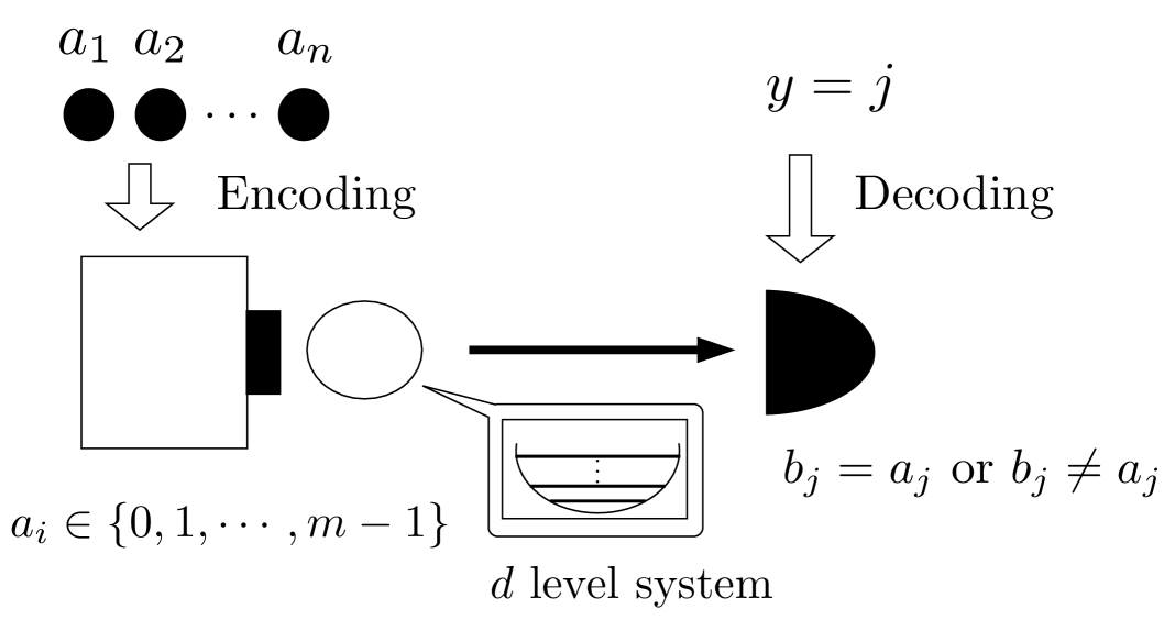
Figure 1: In an $(n,m)$ REC, a sender prepares a message, $a=a_{1}\cdots a_{n}$, of length $n$ where each is chosen from an alphabet of $m$ letters $a_{i}\in\{0,1,\cdots,m-1\}$. An encoding corresponds to a preparation of a single system of cadinality $d$, which is sent to Bob, who first decides which letter he will read, say the $j$-th one, and reads $b_{j}$. Bob wants to exclude the message sent by Alice, i.e., $b_{j}\neq a_{j}$. In RACs, parties want to have $b_{j}=a_{j}$. For these purposes, parties optimize strategies with quantum or classical resources.

We next present a $(2,3)$ REC with single qubit states in the following,

$$\rho_{a}:=\rho_{a_{1}a_{2}}=|\psi_{a_{1}a_{2}}\rangle\langle\psi_{a_{1}a_{2}}|\leavevmode\nobreak\ \mathrm{for}\leavevmode\nobreak\ a_{i}\in\{0,1,2\}$$ (5)

where

$$|\psi_{00}\rangle = \frac{|0\rangle+e^{i\pi/4}|1\rangle}{\sqrt{2}},\leavevmode\nobreak\ \leavevmode\nobreak\ |\psi_{01}\rangle=\frac{|0\rangle+e^{-i\pi/4}|1\rangle}{\sqrt{2}},$$

$$|\psi_{10}\rangle = \frac{|0\rangle+e^{i3\pi/4}|1\rangle}{\sqrt{2}},\leavevmode\nobreak\ \leavevmode\nobreak\ |\psi_{11}\rangle=\frac{|0\rangle+e^{-i3\pi/4}|1\rangle}{\sqrt{2}},$$

$$|\psi_{20}\rangle = \frac{|0\rangle+e^{i\pi/2}|1\rangle}{\sqrt{2}},\leavevmode\nobreak\ \leavevmode\nobreak\ |\psi_{21}\rangle=\frac{|0\rangle+e^{-i\pi/2}|1\rangle}{\sqrt{2}}$$

$$|\psi_{02}\rangle = \frac{|0\rangle+|1\rangle}{\sqrt{2}},\leavevmode\nobreak\ |\psi_{12}\rangle=\frac{|0\rangle-|1\rangle}{\sqrt{2}},\leavevmode\nobreak\ \mathrm{and}\leavevmode\nobreak\ \rho_{22}=\mathds{1}/2.$$

We construct a decoding with two-outcome measurements,

$$\mathcal{M}_{1}=\{M_{10},M_{11},M_{12}\}\leavevmode\nobreak\ \mathrm{and}\leavevmode\nobreak\ \mathcal{M}_{2}=\{M_{20},M_{21},M_{22}\}\leavevmode\nobreak\ \leavevmode\nobreak\ \leavevmode\nobreak\ \leavevmode\nobreak\$$ (6)

where

$$M_{10}=|+\rangle\langle+|,\leavevmode\nobreak\ M_{11}=|-\rangle\langle-|,\leavevmode\nobreak\ M_{12}=0$$

$$M_{20}=|+i\rangle\langle+i|,\leavevmode\nobreak\ M_{21}=|-i\rangle\langle-i|,\leavevmode\nobreak\ \mathrm{and}\leavevmode\nobreak\ M_{22}=0,$$

and $|\pm\rangle=(|0\rangle\pm|1\rangle)/\sqrt{2}$ and $|\pm i\rangle=(|0\rangle\pm i|1\rangle)/\sqrt{2}$. Notice that the states and measurements above are on a half-plane in a Bloch sphere.

The quantum protocol works as follows. Alice sends a state $\rho_{a_{1}a_{2}}$ and Bob first decides which one, $a_{1}$ or $a_{2}$, he is going to read. For the first trit $a_{1}$, he applies measurement $\mathcal{M}_{1}$, and for the second, $a_{2}$, he applies $\mathcal{M}_{2}$. The probability of successfully excluding a one-bit message of Alice is given by,

$$p^{\mathrm{(REC)}}_{Q} = \frac{1}{18}\sum_{a}\sum_{i=1}^{2}{\rm Tr}[(M_{i(a_{i}\oplus 1)}+M_{i(a_{i}\oplus 2)})\leavevmode\nobreak\ \rho_{a_{1}a_{2}}]\leavevmode\nobreak\ \leavevmode\nobreak\$$ (7)

where $\oplus$ represents addition modulo three. It follows that

$$p^{\mathrm{(REC)}}_{Q}=\frac{7+\sqrt{2}}{9}$$ (8)

which is larger than the classical value in Eq. (4). Thus, the usefulness of quantum resources in RECs is shown.

There may exist states and measurements other than those in Eqs. (5) and (6), in particular non-zero positive-operator-value-measure (POVM) elements, such that the success probability is even higher. That is, one can ask if the bound in Eq. (8) is maximal. Our answer is in the affirmative. Firstly, we find that to maximize the success probability with qubit transmission, it suffices to restrict states and measurements to a half-plane on a Bloch sphere. This also holds true even if parties aim at a guessing task, and hence, applies to RACs with qubits. Secondly, extensive numerical optimization of the average success probability finds Eq. (8) with two POVM elements are zeros. We detail the derivations in the Appendix. The gap between quantum and classical bounds is,

$$\Delta_{QC}^{(\mathrm{REC})}=\max_{Q}p^{(\mathrm{REC})}-\max_{C}p^{(\mathrm{REC})}=\frac{\sqrt{2}-1}{9},$$ (9)

which is about $0.046$.

For comparisons, let us also consider a $(2,3)$ RAC with single-qubit transmission. An upper bound to success probabilities with classical strategies is known as $5/9$ Saha et al. (2023). We compute the maximum average probability with quantum resources, applying the aforementioned result of reducing to a half-plane. We find that a relabeling of our quantum protocol for the REC gives the quantum maximum for the RAC; messages $a=a_{1}a_{2}$ are encoded in the states orthogonal to ones given in Eq. (5) and the same measurements as in Eq. (6) are applied for decoding. The quantum bound is obtained as $(4+\sqrt{2})/9$. Interestingly, the gap is identical to Eq. (9), i.e.,

$$\Delta_{QC}^{(\mathrm{RAC})}=\Delta_{QC}^{(\mathrm{REC})}$$ (10)

for the considered $(2,3)$ RAC and $(2,3)$ REC.

In what follows, we are motivated by the observation that a single-shot scenario gives an outcome among possible events. We investigate the minimal quantum and classical resources required to describe possible detection events in the $(2,3)$ REC, and present a dimensional advantage of quantum resources over classical ones. To this end, we exploit communication matrices, a tool that characterizes detection events of a two-party protocol.

A communication matrix is defined for an input $\alpha$ and an outcome $\beta$ as follows Heinosaari and Kerppo (2019); Frenkel and Weiner (2015); Heinosaari et al. (2020),

$$C_{\alpha\beta}={\rm Prob}_{M|P}(\beta|\alpha)$$

where $P$ and $M$ denote preparation and measurement, respectively. For instance, a communication matrix of a guessing task for an alphabet of two letters in a noiseless manner corresponds to a diagonal matrix, $S_{2}=\mathrm{diag}[1,1]$. As for an exclusion task for three letters $\{a,b,c\}$, the communication matrix with the unit success probability is given as

$$A_{3}=\frac{1}{2}\begin{bmatrix}0&1&1\\ 1&0&1\\ 1&1&0\end{bmatrix},$$ (11)

meaning that once a letter is sent, say $a$, a receiver decodes others, i.e., $b$ or $c$, with equal probabilities $1/2$. In the following, we investigate the quantum and classical dimensions required for constructing a communication matrix. We recall that a quantum dimension is referred to as the Hilbert space, and a classical one is defined by the number of distinguishable letters.

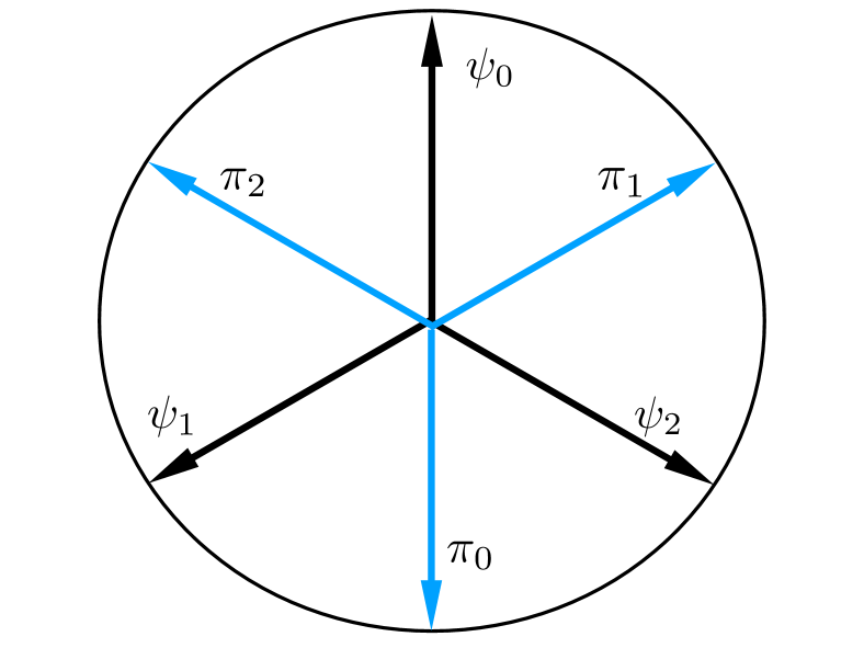
Figure 2: Trine states (black) in Eq. (12) and an anti-trine measurement (blue) in Eq. (13) can realize an unbiased exclusion task, see its communication matrix in Eq. (11). For instance, an outcome $\pi_{0}$ concludes state $\psi_{1}$ or state $\psi_{2}$ with equal probabilities $1/2$ excluding $\psi_{0}$ unambiguously.

To illustrate the approach for quantifying minimal dimensions, let us consider a communication matrix in Eq. (11). A quantum realization can be constructed with trine states, see also Fig. 2

$$|\psi_{\alpha}\rangle=\frac{1}{\sqrt{2}}\left(|0\rangle+e^{i2\pi\alpha/3}|1\rangle\right)\,\,\,\alpha=0,1,2\,,$$ (12)

and anti-trine measurements,

$$\pi_{\beta}=\frac{2}{3}|{\psi}_{\beta}^{\perp}\rangle\langle{\psi}_{\beta}^{\perp}|\,\,\,{\beta}=0,1,2$$ (13)

where $\langle\psi_{k}|{\psi}_{\beta}^{\perp}\rangle=0$. States and measurements above can reproduce a communication matrix in Eq. (11); the Hilbert space of quantum resources has dimension two. Classically, however, it is necessary to have three distinguishable letters to describe the matrix in Eq. (11) as the matrix is of rank three. Therefore, a dimensional advantage of quantum resources is shown.

In general, a communication matrix may have different cardinalities for inputs and outputs. Let us consider an $n\times m$ communication matrix $C$. The minimal dimension of classical resources corresponds to the nonnegative rank, denoted by $\mathrm{rank}_{+}(C)$, as a minimal value of $k$ such that there exist an $n\times k$ nonnegative matrix $L$ and a $k\times m$ nonnegative matrix $R$ that satisfy $LR=C$ Cohen and Rothblum (1993). As for the quantum case, it has been shown that the minimal dimension of quantum resources is given by the positive semidefinite (psd) rank, denoted by $k=\mathrm{rank}_{psd}({C})$, defined as the smallest integer $k$ such that there exists a positive semidefinite $k\times k$ matrices $A_{1},\ldots,A_{n}$ and $B_{1},\ldots,B_{m}$ satisfying $C_{ij}={\rm Tr}[A_{i}B_{j}]$ Fawzi et al. (2015). In the following, we compute the nonnegative and semidefinite ranks of a communication matrix.

The communication matrix for the considered $(2,3)$ REC with the unit success probability, such that exclusion is realized in an unbiased manner, can be obtained as follows,

$$D_{3} =\frac{1}{4}\begin{bmatrix}0&0&0&0&1&1&0&1&1\\ 0&0&0&1&0&1&1&0&1\\ 0&0&0&1&1&0&1&1&0\\ 0&1&1&0&0&0&0&1&1\\ 1&0&1&0&0&0&1&0&1\\ 1&1&0&0&0&0&1&1&0\\ 0&1&1&0&1&1&0&0&0\\ 1&0&1&1&0&1&0&0&0\\ 1&1&0&1&1&0&0&0&0\\ \end{bmatrix}.$$ (14)

It turns out that we have $D_{3}=A_{3}\otimes A_{3}$ and it follows that we have $\mathrm{rank}_{+}(D_{3})=9$ Heinosaari et al. (2020).

A minimal quantum dimension can be found by upper and lower bounds to the positive-semidefinite rank. We consider a quantum realization to ensure an upper bound and then compute a general lower bound. We show that they coincide.

A quantum realization using two qubits is as follows. Alice encodes $a_{1}$ of her string into one qubit, and $a_{2}$ into another, as one of the three trine states in Eq. (12). On receiving the systems, Bob applies an anti-trine measurement (see Eq. (13)) onto the relevant qubit and can hence exclude the state unambiguously. Furthermore, due to the symmetry in the ensemble, the remaining outcomes occur equiprobably. A two-qubit space with a dimension of four, therefore, suffices for the purpose. We have

$$\mathrm{rank}_{psd}(D_{3})\leq 4.$$ (15)

In Ref. Lee et al. (2017), a lower bound to psd ranks for positive doubly stochastic matrices is shown. Applying the bound to $D_{3}$, we have

$$\mathrm{rank}_{psd}({D_{3}})\geq\max_{q}\frac{1}{\sum_{i,j}q_{i}q_{j}F(\mathrm{col}_{i}(D_{3}),\mathrm{col}_{j}(D_{3}))^{2}}$$

where $\mathrm{col}_{i}(D_{3})$ is the $i$-th column of $D_{3}$, the maximum runs over probability vectors $q=[q_{1},\cdots,q_{9}]$ and $F(a,b)=\sum_{i}\sqrt{a_{i}b_{i}}$. We compute that the lower bound is

$$\mathrm{rank}_{psd}({D_{3}})\geq 4,$$

which occurs if $q_{i}=1/9$ for $i=1,\cdots,9$. As upper and lower bounds coincide, we conclude a minimal quantum dimension $4$. The $(2,3)$ REC can be realized on a smaller quantum dimension than a classical one, showing a distinction in quantum and classical supports for detection events.

We also consider quantum and classical dimensions for a $(2,3)$ RAC protocol. Notice that the matrix for noiseless communication is given by

$$\mathbf{1}_{9}=\mathrm{diag}[1,1,1,1,1,1,1,1,1]$$

which is on the support of a dimension $9$. For this matrix, it can be shown that $\mathrm{rank}_{+}(\mathbf{1}_{9})=\mathrm{rank}_{psd}(\mathbf{1}_{9})=9$ Fawzi et al. (2015). Hence, no dimensional advantage is achieved between the quantum and classical dimensions in the RAC. In other words, if a protocol can implement random access perfectly, we can implement exclusion perfectly by relabeling outcomes. The converse, however, is not true: one cannot realize random access with certainty on the quantum support where random exclusion is perfect.

Finally, RECs can be generalized to higher dimensions. We detail in the Appendix the analysis about the $(2,m)$ REC with a single qubit and show quantum advantages for all values of $m\geq 2$. Namely, we have the maximum of the success probability with classical resources,

$$\max_{C}p^{(REC)}=1-\frac{1}{m^{2}}.$$

We extend the quantum strategy considered for $m=3$ to a larger $m$ and have,

$$p_{Q}^{(REC)}=1-\frac{2-\sqrt{2}}{m^{2}},$$

which is strictly higher than the classical one. Thus, quantum advantages remain for all $m\geq 2$.

In conclusion, we have presented a framework for identifying quantum advantages of a single-shot protocol by introducing a communication primitive, RECs, which relies on an exclusion task. A single-shot scenario has a detection event where outcomes occur probabilistically. Quantum advantages are provided by a probability and a dimension. Firstly, the probability that the exclusion task is successful from a single detection event is higher with quantum strategies than with classical ones. Secondly, by exploiting communication matrices, we have shown that the quantum resources of a smaller dimension can realize RECs with a larger alphabet. The dimensional quantum advantage may be lacking in RACs; a protocol for a RAC implies an implementation of a REC by relabeling, but the converse does not hold, similarly to the distinction between state discrimination and state exclusion.

In future directions, it would be interesting to investigate general properties of $(n,m)$ RECs and their relations to quantum state exclusion. In particular, we leave it open to characterize optimal measurements for RECs and quantum state exclusion to find general relations between them. We also conjecture that RECs may have quantum advantages for all $n,m\geq 2$. In addition, it is also interesting to combine the probability and the dimension advantages of quantum resources to amplify the usefulness. We envisage that our results would lead to practical quantum information applications that outperform their classical counterparts.

This work is supported by Business Finland funded project BEQAH, the National Research Foundation of Korea (Grant No. NRF-2021R1A2C2006309, NRF-2022M1A3C2069728, RS-2024-00408613, RS-2023-00257994) and the Institute for Information & Communication Technology Promotion (IITP) (RS-2023-00229524, RS-2025-02304540).

Appendix A Optimal success with classical resource in $(2,3)$ REC

Proposition 1.

The maximum classical average success probability in the simplest random exclusion task, consisting of length $n=2$ words made from size $m=3$ alphabet and dimension of the communicated system $d=2$, is $8/9$.

Proof.

Let us begin by calculating the optimal value over all deterministic protocols. The two stages of a deterministic protocol are as follows: (i) The set of all possible words $\{a_{1}a_{2}:a_{1},a_{2}\in\{0,1,2\}\}$ is partitioned into two parts $\{\mathbb{P}_{0},\mathbb{P}_{1}\}$; if a word to Alice belongs to the part $\mathbb{P}_{0}$ ($\mathbb{P}_{1}$), she communicates to Bob $c=0$ ($c=1$). (ii) Bob, on receiving a question $i\in\{1,2\}$, answers $b_{i}^{c}\in\{0,1,2\}$ following a deterministic strategy, i.e., a map $\{b_{1}^{0},b_{2}^{0},b_{1}^{1},b_{2}^{1}\}\mapsto\{0,1,2\}$.

Let us first note that, for a given deterministic strategy of Bob, two specific words follow, namely, the word $b_{1}^{0}b_{2}^{0}$ and the word $b_{1}^{1}b_{2}^{1}$. Now, let us consider that Alice receives either of these words. The message she communicates will then be determined by her partition, and there are four cases to consider:

1. $b_{1}^{0}b_{2}^{0},b_{1}^{1}b_{2}^{1}\in\mathbb{P}_{0}$,

2. $b_{1}^{0}b_{2}^{0},b_{1}^{1}b_{2}^{1}\in\mathbb{P}_{1}$,

3. $b_{1}^{0}b_{2}^{0}\in\mathbb{P}_{0}$ and $b_{1}^{1}b_{2}^{1}\in\mathbb{P}_{1}$,

4. $b_{1}^{0}b_{2}^{0}\in\mathbb{P}_{1}$ and $b_{1}^{1}b_{2}^{1}\in\mathbb{P}_{0}$.

We study each case in turn. In Case 1, when Alice receives the word $a=b_{1}^{0}b_{2}^{0}$ she will communicate the value $c=0$ to Bob. For each question $i$ that he is asked he will output $b_{i}^{0}$, which was the value he aimed to exclude. Therefore, the protocol fails two times. Note that, in this case, if instead she received the message $a=b_{1}^{1}b_{2}^{1}$, Bob will end up answering $b_{1}^{0}$ and $b_{2}^{0}$ which need not be the same as the initial string; he can therefore succeed in these cases. Case 2 follows the same argument as Case 1. For Case 3, when Alice receives $a=b_{1}^{0}b_{2}^{0}$, her message is $c=0$ and Bob’s output will therefore be $b_{i}^{0}$, so he fails for both questions. Similarly, he will be incorrect whenever $b_{1}^{1}b_{2}^{1}$ is the message received by Alice. Thus, in Case 3, Bob fails in at least four instances of the protocol.

In Case 4, as in Case 3, it can never follow that $b_{1}^{0}b_{2}^{0}=b_{1}^{1}b_{2}^{1}$ as this would mean that Alice puts the same word into two sides of the partition. Let us first suppose that $b_{1}^{0}b_{2}^{1}\neq b_{2}^{0}b_{1}^{1}$. Then, when Alice receives $a=b_{1}^{0}b_{2}^{1}$ she will communicate either $c=0$ or $c=1$ depending on which partition it belongs to. In the former case, Bob’s answer is in the string when his question is $i=1$ and in the latter case it is in the string when his question is $i=0$. Similarly, he will be incorrect in at least one position $i$ when the initial string is $a=b_{2}^{0}b_{1}^{1}$. Case 4 therefore fails at least four times if $b_{1}^{0}b_{2}^{0}=b_{1}^{1}b_{2}^{1}$. The final situation is that $b_{1}^{0}b_{2}^{1}=b_{2}^{0}b_{1}^{1}$. This implies further that $b_{1}^{0}=b_{2}^{0}$ and $b_{1}^{1}=b_{2}^{1}$. On considering the words $a=b_{1}^{0}b_{1}^{1}$ and $a=b_{1}^{1}b_{1}^{0}$ , irrespective of which partition they belong to the protocol will fail at least once for each. Therefore, in Case 4 as well it is observed that the protocol fails to exclude in at least two instances.

We can hence see that, in all four cases, for any deterministic strategy Bob answers incorrectly in at least two out of eighteen instances of the protocol. The maximal average success probability with deterministic strategies is therefore upper bounded by ${p}^{\mathrm{(REC)}}\leq 16/18=8/9$. This bound is, in fact, tight and can be achieved if Alice uses the partition $\mathbb{P}_{0}=\{11,12,21,22\}$ and $\mathbb{P}_{1}=\{00,01,02,10,20\}$, and if Bob’s decoding is $b_{i}^{c}=c$. One can easily verify that this strategy gives the desired value.

Finally, we show that probabilistic strategies cannot perform better. Let’s assume that there are $K$ deterministic strategies $S_{j}$ where $j\in\{1,\cdots,K\}$ and the parties have access to shared random variables $\{\lambda_{j}\}_{j=1}^{K}$ with probability distribution $p(\lambda_{j})=p_{j}$. Note that any probabilistic strategy can be implemented with access to these random variables. If Alice and Bob apply strategy $S_{j}$ with probability $p_{j}$ we get a probabilistic strategy $S=\{p_{j},S_{j}\}_{j=1}^{K}$. The average success probability with any such strategy $S$ is ${p}^{\mathrm{(REC)}}_{S}=\sum_{j}p_{j}{p}^{\mathrm{(REC)}}_{S_{j}}\leq\sum_{j}p_{j}(8/9)=8/9$. This completes the proof. ∎

Appendix B Maximum quantum success probability in $(2,3)$ REC

Proposition 2.

The maximum average success probability in the quantum random exclusion task for a two-outcome POVM is $\frac{7+\sqrt{2}}{9}$.

Proof.

Without loss of generality, we consider the two 2-outcome POVMs applied in the protocol are: $M_{1}\equiv M_{10}+M_{11}=\mathbb{I}$  (we take $M_{12}=0$) and $M_{2}\equiv M_{20}+M_{21}=\mathbb{I}$  (we take $M_{22}=0$). Let us partition the set of all words $a=a_{1}a_{2}\in\mathcal{A}^{2}$ into two parts: $\mathbb{P}=\{00,01,10,11\}$ and $\mathbb{P}^{c}=\{02,20,12,21,22\}$. Then, from the Eq. (7) we get

$${p}^{\mathrm{(REC)}}_{Q} \!=\!\frac{1}{18}\sum_{a}\sum_{i=1}^{2}{\rm Tr}[(\mathbb{I}-M_{ia_{i}})\rho_{a_{1}a_{2}}]$$

$$=\frac{4}{9}\left\{\frac{1}{8}\sum\limits_{a\in\mathbb{P}}\sum\limits_{i=1}^{2}{\rm Tr}\left[(\mathbb{I}-M_{ia_{i}})\rho_{a_{1}a_{2}}\right]\right\}$$

$$+\frac{1}{18}\sum\limits_{a\in\mathbb{P}^{c}}\left\{\sum\limits_{i=1}^{2}{\rm Tr}[(\mathbb{I}-M_{ia_{i}})\rho_{a_{1}a_{2}}]\right\}$$

$$\leq\frac{4}{9}\left\{\frac{1}{8}\sum\limits_{a\in\mathbb{P}}\sum\limits_{i=1}^{2}{\rm Tr}\left[(\mathbb{I}-M_{ia_{i}})\rho_{a_{1}a_{2}}\right]\right\}+\frac{5}{9}$$

$$\leq\frac{4}{9}\left\{\max\limits_{\{\begin{subarray}{c}M_{ia_{i}},\\ \rho_{a_{1}a_{2}}\end{subarray}\}}\leavevmode\nobreak\ \frac{1}{8}\sum\limits_{a\in\mathbb{P}}\sum\limits_{i=1}^{2}{\rm Tr}\left[(\mathbb{I}-M_{ia_{i}})\rho_{a_{1}a_{2}}\right]\right\}\!+\!\frac{5}{9}$$

$$=\frac{4}{9}\left\{\max\limits_{\{\begin{subarray}{c}\tilde{M}_{ia_{i}},\\ \rho_{a_{1}a_{2}}\end{subarray}\}}\leavevmode\nobreak\ \frac{1}{8}\sum\limits_{a\in\mathbb{P}}\sum\limits_{i=1}^{2}{\rm Tr}\left[\tilde{M}_{ia_{i}}\leavevmode\nobreak\ \rho_{a_{1}a_{2}}\right]\right\}+\frac{5}{9}$$

$$\leavevmode\nobreak\ \leavevmode\nobreak\ \leavevmode\nobreak\ \leavevmode\nobreak\ \leavevmode\nobreak\ \leavevmode\nobreak\ \leavevmode\nobreak\ (\mbox{we\leavevmode\nobreak\ rewrite}\leavevmode\nobreak\ \mathbb{I}-M_{ia_{i}}=\tilde{M}_{ia_{i}}\leavevmode\nobreak\ ),$$

$$\leq\frac{4}{9}\left\{\frac{1}{2}\left(1+\frac{1}{\sqrt{2}}\right)\right\}+\frac{5}{9}=\frac{7+\sqrt{2}}{9}.$$ (16)

In the last step above, we simply apply the known result, i.e., in a $(2,2)$ RAC, the quantum maximum for the average success probability is $(1+1/\sqrt{2})/2$. Since our quantum protocol reaches the derived quantum upper bound, we find an optimal over the set of all two-outcome measurement protocols.

∎

In general, the optimization problem consists of maximizing the figure of merit over all possible three-outcome POVMs on a qubit space. To find optimal states and measurements for the purpose, let us rewrite the average success probability as follows,

$${p}^{\mathrm{(REC)}}_{Q} = \frac{1}{36}\sum_{a}{\rm Tr}[\sum_{i=1}^{2}[(\mathbb{I}-M_{ia_{i}})\otimes\rho_{a_{1}a_{2}}^{T})|\phi^{+}\rangle\langle\phi^{+}|],$$

where $|\phi^{+}\rangle=(|00\rangle+|11\rangle)/\sqrt{2}$. Note that a state $|\phi^{+}\rangle$ is permutationally invariant, which means that the states and the measurements that maximise the success probability should be in a symmetric subspace, supported by a quantum $2$-design. This implies that optimal states and measurements fulfil the condition,

$$\sum_{i=1}^{2}(\mathbb{I}-M_{ia_{i}})\propto\rho_{a_{1}a_{2}}^{*}.$$ (17)

Applying the above, we will then show that to achieve the maximal success probability, it is sufficient to optimize a function which depends only on the measurement parameters (i.e., for any given decoding measurements, one can always choose an optimal set of states derived from the measurement). All these simplify the construction of states and measurements.

First, recall that we need to maximize ${p}^{\mathrm{(REC)}}_{Q}$ in Eq. (7) in the main text. From the objective function, one can see that the maximum is achieved with extremal (pure) states and measurements. Then let us consider a set of nine pure qubit states

$$\rho_{a_{1}a_{2}} = \frac{1}{2}(\mathbb{I}+\hat{n}_{a_{1}a_{2}}\cdot\vec{\sigma}),$$ (18)

where $\hat{n}_{a_{1}a_{2}}$ for $a_{1},a_{2}\in\{0,1,2\}$ are unit vectors on the Bloch sphere, and two measurements corresponding to extremal POVMs which are given by rank one projectors, i.e.,

$$M_{1a_{1}} = r_{1a_{1}}\left(\frac{\mathbb{I}+\hat{m}_{1a_{1}}\cdot\vec{\sigma}}{2}\right),$$ (19)

$$M_{2a_{2}} = r_{2a_{2}}\left(\frac{\mathbb{I}+\hat{m}_{2a_{2}}\cdot\vec{\sigma}}{2}\right),$$ (20)

where $\hat{m}_{1a_{1}}$ ($\hat{m}_{2a_{2}}$) are unit vectors on the Bloch sphere in a plane passing through the origin such that weights $0\leq r_{1a_{1}}\leq 1$ ($0\leq r_{2a_{2}}\leq 1$) and $\sum_{a_{1}}r_{1a_{1}}=2$  ($\sum_{a_{2}}r_{2a_{2}}=2$). On rearranging the terms in ${p}^{\mathrm{(REC)}}_{Q}$ in Eq. (7), the expression for quantum success probability becomes

$${p}^{\mathrm{(REC)}}_{Q} = 1-\frac{1}{18}\sum_{a}{\rm Tr}\left[(M_{1a_{1}}+M_{2a_{2}})\rho_{a_{1}a_{2}}\right]$$

$$= \frac{2}{3}-\frac{1}{36}\sum_{a}\left\{\hat{n}_{a_{1}a_{2}}\cdot(r_{1a_{1}}\hat{m}_{1a_{1}}+r_{2a_{2}}\hat{m}_{2a_{2}})\right\},$$

then application of Eq. (17) gives

$${p}^{\mathrm{(REC)}}_{Q} \leq \frac{2}{3}+\frac{1}{36}\leavevmode\nobreak\ \sum_{a}|r_{1a_{1}}\!\hat{m}_{1a_{1}}\!+\!r_{2a_{2}}\hat{m}_{2a_{2}}|.$$ (21)

Note that very similar to the the considered REC task, on analysing the corresponding RAC, through Eq. (2), for maximum quantum success, we get an achievable upper bound function as follows:

$${p}^{\mathrm{(RAC)}}_{Q} \leq \frac{1}{3}+\frac{1}{36}\leavevmode\nobreak\ \sum_{a}|r_{1a_{1}}\!\hat{m}_{1a_{1}}\!+\!r_{2a_{2}}\hat{m}_{2a_{2}}|.$$ (22)

Thus, the optimization problems both for the quantum REC and RAC reduces to maximizing the same objective function.

From the steps above one can easily see that for arbitrarily fixed measurements, one can always choose states such that the upper bound is attained. Therefore, it is sufficient to maximize the quantity

$$f\! = \!\sum_{a_{2}\!=\!0}^{2}\!\sum_{a_{1}\!=\!0}^{2}|r_{1a_{1}}\hat{m}_{1a_{1}}\!+\!r_{2a_{2}}\hat{m}_{2a_{2}}|,$$

$$= \!\sum_{a_{2}\!=\!0}^{2}\!\sum_{a_{1}\!=\!0}^{2}\!\!\left\{r_{1a_{1}}^{2}\!\!+\!r_{2a_{2}}^{2}\!\!+\!2r_{1a_{1}}\!r_{2a_{2}}\!\cos(\phi_{1a_{1}}\!\!-\!\phi_{2a_{2}})\sin\theta_{2a_{2}}\right\}^{\frac{1}{2}},$$

which is a function of the two measurements derived from the extremal POVMs $M_{i}$, where $i\in\{1,2\}$ and $(\theta_{ia_{i}},\phi_{ia_{i}})$ are spherical polar coordinates of the Bloch vector $\hat{m}_{ia_{i}}$. The weight parameters of the three-outcome (corresponding to indices $\kappa\in\{0,1,2\}$) POVMs, can be written by

$$r_{i\kappa}\! = \!\frac{2\sin\alpha_{i\kappa}}{\sin\alpha_{i0}\!+\!\sin\alpha_{i1}\!+\!\sin\alpha_{i2}},$$ (24)

$$\alpha_{i0}+\alpha_{i1}+\alpha_{i2}=2\pi,$$ (25)

$$0\leq\alpha_{i0},\leavevmode\nobreak\ \alpha_{i1},\leavevmode\nobreak\ \alpha_{i2}\leq\pi.$$ (26)

See Fig. 3 to visualize the measurements.

Figure 3: Illustration of a three-outcome extremal POVM (on a qubit) on a plane passing through the origin of the Bloch sphere.

In general, the Bloch vectors corresponding to two different measurements may live in two different planes. We choose, without loss of generality, the Bloch plane of the measurement $M_{1}$ as the $XY$-plane. We choose the $Y$-axis along the line where the planes of the two measurements $M_{1}$ and $M_{2}$ intersect. Let us denote angle of the unit vector normal to the plane of the measurement $M_{2}$ with the $Z$-axis by $0\leq\Theta\leq\pi$. Further, without loss of generality, for the second measurement $M_{2}$ we set the angle of the Bloch vector of the first outcome $\phi_{20}=0$, and for the first measurement let us denote the angle of the Bloch vector of the first outcome $\phi_{10}=\Phi$. Now the objective function in Eq. (LABEL:eq:f) can be re-written in terms of the variables $\alpha_{ia_{i}}$, $\Theta$, and $\Phi$ by applying Eq. (24) and transforming the variables $(\theta_{ia_{i}},\phi_{ia_{i}})$ to the new variables.

Let us then choose a vector orthonormal to the plane $M_{2}$ as $\hat{\mathbf{n}}_{2}=(-\sin\Theta,\leavevmode\nobreak\ 0,\leavevmode\nobreak\ \cos\Theta)$ and a reference vector in the plane $M_{2}$ as $\hat{\mathbf{p}}_{2}=(\sin(\pi/2-\Theta),\leavevmode\nobreak\ 0,\leavevmode\nobreak\ \cos(\pi/2-\Theta))$. The Bloch vectors of the POVM elements $M_{2j}$, where $j\in\{0,1,2\}$ is given by

$$\hat{m}_{2j}=(\sin\theta_{2j}\cos\phi_{2j},\leavevmode\nobreak\ \sin\theta_{2j}\sin\phi_{2j},\leavevmode\nobreak\ \cos\theta_{2j})$$ (27)

One can solve the system of equations

$$\hat{\mathbf{n}}_{2}\cdot\hat{m}_{2j} = 0$$ (28)

$$\hat{\mathbf{p}}_{2}\cdot\hat{m}_{2j} = \cos\alpha_{2j}$$ (29)

to find the variables $\theta_{2j}$ and $\phi_{2j}$ in terms of the variable $\Theta$ and $\alpha_{2j}$. Thus, the objective function $f$ in Eq. (LABEL:eq:f) is now written in terms of six free variables: i.e., $f(\Theta,\Phi,\alpha_{10},\alpha_{12},\alpha_{20},\alpha_{22})$ (here we have applied Eq. (25) to eliminate the two dependent variables $\alpha_{11}$ and $\alpha_{21}$). Then the following proposition holds.

Proposition 3.

The optimal value of $f$ in Eq. (LABEL:eq:f) is achieved with both the three outcome POVMs $M_{1}$ and $M_{2}$ in the $XY$-plane of the Bloch sphere, that is, when variable $\Theta=0$.

Proof.

—We omit the lengthy expressions and steps, but the idea is simple. Objective function in Eq. (LABEL:eq:f) is written in terms of $\Theta$ and the remaining variables. Then we analyze the effect of changing the angle $\Theta$ (angle between the two measurement planes). This is done by taking the partial derivative of the objective function $f$ with respect to the variable $\Theta$. We find that for an arbitrarily fixed value of all the other variables, the partial derivative with respect to $\Theta$ is either always nonnegative or always nonpositive, i.e., the function is either increasing or decreasing. Then a maximum (for any fixed value of all the other variables) will be achieved at an end point in the interval $0\leq\Theta\leq\pi$, implying that the optimal measurement $M_{2}$ lies in the $XY$-plane of the Bloch sphere (i.e., both the measurements are in the same plane). ∎

Applying the above lemma, now the optimization problem is reduced to maximizing

$$\!\!\!\!\!\!f^{\ast}\! = \!\!\sum_{a_{2}\!=\!0}^{2}\!\sum_{a_{1}\!=\!0}^{2}\!\!\left\{\!r_{1a_{1}}^{2}\!\!+\!r_{2a_{2}}^{2}\!\!+\!2r_{1a_{1}}\!r_{2a_{2}}\!\cos(\phi_{1a_{1}}\!\!-\!\phi_{2a_{2}})\right\}^{\frac{1}{2}\!}$$

where both the three outcome measurements are from the $XY$-plane. In Fig. (4) two three outcome extremal POVMs in the XY-plane is shown.

Figure 4: Illustration of three outcome extremal POVMs on the $XY$-plane of the Bloch sphere.

In Eq. (LABEL:eq:fstar), for $i\in\{1,2\}$, we substitute

$$r_{i0} = \frac{2\sin\alpha_{i0}}{\sin\alpha_{i0}-\sin(\alpha_{i0}+\alpha_{i2})+\sin\alpha_{i2}},$$ (31)

$$r_{i1} = \frac{-2\sin(\alpha_{i0}+\alpha_{i2})}{\sin\alpha_{i0}-\sin(\alpha_{i0}+\alpha_{i2})+\sin\alpha_{i2}},$$ (32)

$$r_{i2} = \frac{2\sin\alpha_{i2}}{\sin\alpha_{i0}-\sin(\alpha_{i0}+\alpha_{i2})+\sin\alpha_{i2}};$$ (33)

$$\phi_{i0} = (2-i)\leavevmode\nobreak\ \Phi,$$ (34)

$$\phi_{i1} = (2-i)\leavevmode\nobreak\ \Phi+\alpha_{i2},$$ (35)

$$\phi_{i2} = (2-i)\leavevmode\nobreak\ \Phi+\alpha_{i2}+\alpha_{i0}.$$ (36)

The free variables in the optimization problem are now explicit; constraints on these variables are given by

$$0\leq\alpha_{i0},\leavevmode\nobreak\ \alpha_{i2}\leq\pi\leavevmode\nobreak\ \mbox{and}\leavevmode\nobreak\ \pi\leq\alpha_{i0}+\alpha_{i2}\leq 2\pi,$$ (37)

$$0\leq\Phi\leq\pi.$$ (38)

Proposition 4.

The optimal value of $f^{\ast}$ in Eq. (LABEL:eq:fstar) is given by $4(1+\sqrt{2})$ and it is achieved when both measurements $M_{1}$ and $M_{2}$ are two outcome projective measurements in orthogonal directions. Consequently, the optimal quantum success probability for the REC task is $(7+\sqrt{2})/9$ (and that for the corresponding RAC task is $(4+\sqrt{2})/9$); in particular, the quantum protocol presented in the main text is an optimal one for the REC task.

Our proposition is supported by our analytical simplification (reduction) of the optimization problem stated in proposition (3), followed by numerical optimization implemented on Mathematica. We get an approximate maximum value $\max(f^{\ast})\approx 9.65685\approx 4(1+\sqrt{2})$.

Appendix C Bounds on random exclusion task for alphabet size m

Proposition 5.

The maximum classical average success probability for the random exclusion task with alphabet size $m$ is $\max_{C}\leavevmode\nobreak\ {p}^{\mathrm{(REC)}}=(1-\frac{1}{m^{2}})$.

Proof.

Let us first find the optimal value over all the deterministic protocols. The two stages of any deterministic protocol are as follows. (i) Alice sending one bit information $c\in\{0,1\}$ corresponds to some two partition $\mathbb{P}_{0},\mathbb{P}_{1}$ of the set of all possible words $\mathcal{A}^{2}:=\{a_{1}a_{2}:a_{1},a_{2}\in\{0,1,2,\dots,m-1\}\}$; if the received word $a=a_{1}a_{2}\in\mathbb{P}_{0}$, Alice communicates $c=0$ to Bob, otherwise she sends $c=1$. (ii) Bob’s answer depends on the received bit, he answers with, say, $b_{i}^{c}\in\{0,1,2,\dots,m-1\}$, i.e., Bob’s deterministic strategy corresponds to assigning values to $b_{1}^{0},b_{2}^{0},\leavevmode\nobreak\ b_{1}^{1},b_{2}^{1}\in\{0,1,2,\dots,m-1\}$.

First we show that for any deterministic strategy of Alice and Bob, for at least two out of the total $2m^{2}$ possible instances ($m^{2}$ possible words to Alice and two possible questions to Bob), Bob’s answers will be incorrect. To show this, first, we note that from any deterministic strategy of Bob one can derive the following two words $b_{1}^{0}b_{2}^{0},b_{1}^{1}b_{2}^{1}\in\mathcal{A}^{2}$, therefore, for these two words, given a deterministic strategy of Alice, there are four possibilities:

1. $b_{1}^{0}b_{2}^{0},\leavevmode\nobreak\ b_{1}^{1}b_{2}^{1}\in\mathbb{P}_{0}$,

2. $b_{1}^{0}b_{2}^{0},\leavevmode\nobreak\ b_{1}^{1}b_{2}^{1}\in\mathbb{P}_{1}$,

3. $b_{1}^{0}b_{2}^{0}\in\mathbb{P}_{0}$ and $b_{1}^{1}b_{2}^{1}\in\mathbb{P}_{1}$,

4. $b_{1}^{0}b_{2}^{0}\in\mathbb{P}_{1}$ and $b_{1}^{1}b_{2}^{1}\in\mathbb{P}_{0}$.

In the case-1, when Alice receives the word $b_{1}^{0}b_{2}^{0}$, Bob’s answer is $b_{i}^{0}$ which is incorrect at both the positions $i\in\{1,2\}$. In case-2, similar to case-1, when Alice receives the word $b_{1}^{1}b_{2}^{1}$, Bob’s answer is $b_{i}^{1}$ which is incorrect at both the positions $i\in\{1,2\}$.

In case-3 and case-4 it can never happen that $b_{1}^{0}b_{2}^{0}=b_{1}^{1}b_{2}^{1}$ because same word cannot appear in two distinct partitions.

For the case-3, when Alice receives the word $b_{1}^{0}b_{2}^{0}$ ($b_{1}^{1}b_{2}^{1}$), Bob’s answer is $b_{i}^{0}$ ($b_{i}^{1}$) which is incorrect at both the positions $i\in\{1,2\}$; thus in the case-3 Bob answers incorrectly in at least four instances, namely $b_{1}^{0}b_{2}^{0},b_{1}^{1}b_{2}^{1}$.

Lastly, in the case-4, first suppose that $b_{1}^{0}b_{2}^{1}\neq b_{2}^{0}b_{1}^{1}$. Then for the word $b_{1}^{0}b_{2}^{1}$, to whichever partition it belongs, Bob’s answer will be incorrect at least at one position $i\in\{1,2\}$; similarly, for the word $b_{2}^{0}b_{1}^{1}$, to whichever partition it belongs, Bob’s answer will be incorrect at least at one position $i\in\{1,2\}$. In the remaining situation, i.e., $b_{1}^{0}b_{2}^{1}=b_{2}^{0}b_{1}^{1}\Leftrightarrow b_{1}^{0}=b_{2}^{0}\leavevmode\nobreak\ \mbox{and}\leavevmode\nobreak\ b_{1}^{1}=b_{2}^{1}$, on considering the words $b_{1}^{0}b_{1}^{1}$ and $b_{1}^{1}b_{1}^{0}$ (irrespective which partition they belong to) Bob’s answer is incorrect at least two times; at least once for the first word $b_{1}^{0}b_{1}^{1}$ and at least once for the second word $b_{1}^{1}b_{1}^{0}$. Then, in case-4 as well, Bob’s answer is incorrect in least in two instances.

Therefore, in all the four cases, we get that for any deterministic strategy of Alice and Bob, in at least two out of $2m^{2}$ cases Bob answers incorrectly. Therefore, maximal average success probability with deterministic strategies is upper bounded by $\frac{2m^{2}-2}{2m^{2}}=1-\frac{1}{m^{2}}$.

Finally, we show that probabilistic strategies cannot do better. Lets say there are total $N$ number of deterministic strategies $S_{j}$ where $j\in\{1,\cdots,N\}$. Suppose, Alice and Bob have shared random variables $\{\lambda_{j}\}_{j=1}^{N}$ with probability distribution $p(\lambda_{j})=p_{j}$. Note that any probabilistic strategy can be implemented with an access to the considered shared random variables. Then if Alice and Bob apply strategy $S_{j}$ with probability $p_{j}$ we get a probabilistic strategy $S=\{p_{j},S_{j}\}_{j=1}^{N}$. Then the average success probability with any such strategy $S$ is ${p}^{\mathrm{(REC)}}_{S}=\sum_{j}p_{j}{p}^{\mathrm{(REC)}}_{S_{j}}\leq\sum_{j}p_{j}\left(1-\frac{1}{m^{2}}\right)=1-\frac{1}{m^{2}}$. This completes the proof. ∎

Quantum advantage.— Here we will show that there is a quantum protocol which considers only two outcome measurements for decoding to beat the optimal classical value derived above. Alice sends the information on her words $a_{1}a_{2}$ by encoding in a one qubit state $\rho_{a_{1}a_{2}}$ as follows:

$$\rho_{00} =\frac{1}{2}\left(\mathbb{I}+\sigma_{x}\right), \rho_{01} =\frac{1}{2}\left(\mathbb{I}+\sigma_{z}\right), \rho_{0c_{2}} =\frac{1}{2}\left(\mathbb{I}+\frac{\sigma_{x}+\sigma_{z}}{\sqrt{2}}\right)$$

$$\rho_{10} =\frac{1}{2}\left(\mathbb{I}-\sigma_{z}\right), \rho_{11} =\frac{1}{2}\left(\mathbb{I}-\sigma_{x}\right), \rho_{1c_{2}} =\frac{1}{2}\left(\mathbb{I}-\frac{\sigma_{x}+\sigma_{z}}{\sqrt{2}}\right)$$

$$\rho_{c_{1}0} =\frac{1}{2}\left(\mathbb{I}+\frac{\sigma_{x}-\sigma_{z}}{\sqrt{2}}\right), \rho_{c_{1}1} =\frac{1}{2}\left(\mathbb{I}+\frac{\sigma_{z}-\sigma_{x}}{\sqrt{2}}\right), \rho_{c_{1}c_{2}} =\frac{\mathbb{I}}{2}$$

$$\text{where }c_{1},c_{2} \in\{2,3,\ldots,m-1\}.$$ (39)

All the qubit states used for encoding are from the $XZ$-plane of the Bloch sphere. To answer the first position in the Alice’s word, Bob performs a two outcome projective measurement $\mathcal{M}_{1}$; on measurement outcome $+1$ ($-1$) he answers $0$ ($1$). Whereas for answering the second position he measures $\mathcal{M}_{2}$ and answers with $0$ ($1$) when the measurement outcome is $+1$ ($-1$). The average success probability of our protocol is

$${p}^{\mathrm{(REC)}}_{Q} := 1-\frac{1}{2m^{2}}\sum_{a_{1},a_{2}\in\mathcal{A}}\leavevmode\nobreak\ \mbox{Tr}\left[\rho_{a_{1}a_{2}}\left(M_{1a_{1}}+M_{2a_{2}}\right)\right]$$

$$= 1-\frac{2-\sqrt{2}}{m^{2}}.$$

Here the first and second measurements are implemented as follows

$$\mathcal{M}_{1} \equiv \left\{M_{10}=\frac{1}{2}\left(\mathbb{I}-\frac{\sigma_{x}+\sigma_{z}}{\sqrt{2}}\right),\leavevmode\nobreak\ M_{11}=\frac{1}{2}\left(\mathbb{I}+\frac{\sigma_{x}+\sigma_{z}}{\sqrt{2}}\right),\leavevmode\nobreak\ M_{1c_{1}}=0\right\},$$

$$\mathcal{M}_{2} \equiv \left\{M_{20}=\frac{1}{2}\left(\mathbb{I}+\frac{\sigma_{z}-\sigma_{x}}{\sqrt{2}}\right),\leavevmode\nobreak\ M_{21}=\frac{1}{2}\left(\mathbb{I}+\frac{\sigma_{x}-\sigma_{z}}{\sqrt{2}}\right),\leavevmode\nobreak\ M_{2c_{2}}=0\right\}.$$ (40)

Note that Bob never answers $\{2,3,\ldots,m-1\}$, still our protocol gives a high success because the goal here is to answer with alphabet different from those appearing in the words. Also note that the state $\rho_{c_{1}c_{2}}$ used for encoding the words $c_{1}\;c_{2}$, can be any arbitrary state, even any mixed state, e.g., maximally mixed state $\frac{\mathbb{I}}{2}$. This is due to the fact $M_{1c_{1}}=0$ and $M_{2c_{2}}=0$, i.e., outcomes $c_{1}\text{ or }c_{2}$ never occur for the considered measurements.

Proposition 6.

The maximum average success probability in the quantum random exclusion task, with alphabet size $m$, for a two-outcome POVM is achieved with the above discussed quantum protocol.

Proof.

Let us address the scenario wherein Alice sends a qubit instead of a bit. We can show that there is a quantum advantage in this case for all $m$. The proof of advantage only requires Bob to perform two 2-outcome measurements. Say we form the partition as $\mathbb{Q}=\{00,01,10,11\}$ and $\overline{\mathbb{Q}}=\{a_{1}a_{2}\in\mathcal{A}^{2}:a_{1}a_{2}\notin\mathbb{Q}\}$. The two 2-outcome measurements can be used to distinguish between states associated with $\mathbb{Q}$. For the states associated with $\overline{\mathbb{Q}}$, the measurement output is always correct for our task. We can find an upperbound for the quantum success probability as well:

$${p}^{\mathrm{(REC)}}_{Q} =\frac{1}{2m^{2}}\sum_{a\in\mathcal{A}^{2}}\sum_{i=1}^{2}{\rm Tr}\left[(\mathbb{I}-M_{ia_{i}})\rho_{a_{1}a_{2}}\right]$$

$$=\frac{4}{m^{2}}\left\{\frac{1}{8}\sum\limits_{a\in\mathbb{Q}}\sum\limits_{i=1}^{2}{\rm Tr}\left[(\mathbb{I}-M_{ia_{i}})\rho_{a_{1}a_{2}}\right]\right\}+\frac{1}{2m^{2}}\sum\limits_{a\in\overline{\mathbb{Q}}}\left\{\sum\limits_{i=1}^{2}{\rm Tr}[(\mathbb{I}-M_{ia_{i}})\rho_{a_{1}a_{2}}]\right\}$$

$$\leq\frac{4}{m^{2}}\left\{\frac{1}{8}\sum\limits_{a\in\mathbb{Q}}\sum\limits_{i=1}^{2}{\rm Tr}\left[(\mathbb{I}-M_{ia_{i}})\rho_{a_{1}a_{2}}\right]\right\}+\frac{m^{2}-4}{m^{2}}$$

$$\leq\frac{4}{m^{2}}\left\{\max\limits_{\{M_{ia_{i}},\leavevmode\nobreak\ \rho_{a_{1}a_{2}}\}}\leavevmode\nobreak\ \frac{1}{8}\sum\limits_{a\in\mathbb{Q}}\sum\limits_{i=1}^{2}{\rm Tr}\left[(\mathbb{I}-M_{ia_{i}})\rho_{a_{1}a_{2}}\right]\right\}+\frac{m^{2}-4}{m^{2}}$$

$$=\frac{4}{m^{2}}\left\{\max\limits_{\{\tilde{M}_{ia_{i}},\leavevmode\nobreak\ \rho_{a_{1}a_{2}}\}}\leavevmode\nobreak\ \frac{1}{8}\sum\limits_{a\in\mathbb{Q}}\sum\limits_{i=1}^{2}{\rm Tr}\left[\tilde{M}_{ia_{i}}\leavevmode\nobreak\ \rho_{a_{1}a_{2}}\right]\right\}+\frac{m^{2}-4}{m^{2}}\leavevmode\nobreak\ \leavevmode\nobreak\ \leavevmode\nobreak\ \leavevmode\nobreak\ (\leavevmode\nobreak\ \mbox{here}\leavevmode\nobreak\ \tilde{M}_{ia_{i}}=\mathbb{I}-M_{ia_{i}}\leavevmode\nobreak\ ),$$

$$\leq\frac{4}{m^{2}}\left\{\frac{1}{2}\left(1+\frac{1}{\sqrt{2}}\right)\right\}+\frac{m^{2}-4}{m^{2}}$$

$$=1-\frac{2-\sqrt{2}}{m^{2}}.$$

In the last step above, we simply apply the known result, i.e., in a $2\rightarrow 1$ random access codes the quantum maximum for the average success probability is $(1+1/\sqrt{2})/2$. Since our quantum protocol reaches the derived quantum upper bound, we find an optimal over the set of all two-outcome measurement protocols. ∎

With this result, we can see that, as long as Alice is only using a two level system to communicate to Bob, Alice can achieve a quantum advantage for any finite alphabet size $m$ of Alice’s input since $1-\frac{2-\sqrt{2}}{m^{2}}>1-\frac{1}{m^{2}}$.

References

- Winter (2013) A. Winter, ”Winter’s Principle”, Benasque (2013).
- Holevo (2011) A. S. Holevo, Probabilistic and statistical aspects of quantum theory, Publications of the Scuola Normale Superiore (Scuola Normale Superiore, Pisa, Italy, 2011).
- Holevo (1998) A. Holevo, IEEE Transactions on Information Theory 44, 269 (1998).
- Schumacher and Westmoreland (1997) B. Schumacher and M. D. Westmoreland, Phys. Rev. A 56, 131 (1997).
- Ambainis et al. (2009) A. Ambainis, D. Leung, L. Mancinska, and M. Ozols, (2009), arXiv:0810.2937 [quant-ph] .
- Ambainis et al. (2024) A. Ambainis, D. Kravchenko, S. Sazim, J. Bae, and A. Rai, New J. Phys. 26, 123023 (2024).
- Tavakoli et al. (2015) A. Tavakoli, A. Hameedi, B. Marques, and M. Bourennane, Phys. Rev. Lett. 114, 170502 (2015).
- Carmeli et al. (2020) C. Carmeli, T. Heinosaari, and A. Toigo, Europhysics Lett. 130, 50001 (2020).
- Helstrom (1969) C. W. Helstrom, Journal of Statistical Physics 1, 231 (1969).
- Bae and Kwek (2015) J. Bae and L.-C. Kwek, J. Phys. A: Math. Theor. 48, 083001 (2015).
- Barnett and Croke (2009) S. M. Barnett and S. Croke, Adv. Opt. Photon. 1, 238 (2009).
- Bergou (2007) J. A. Bergou, Journal of Physics: Conference Series 84, 012001 (2007).
- Caves et al. (2002) C. M. Caves, C. A. Fuchs, and R. Schack, Phys. Rev. A 66 (2002).
- Pusey et al. (2012) M. Pusey, J. Barrett, and T. Rudolph, Nature Physics 8, 475 (2012).
- Bandyopadhyay et al. (2014a) S. Bandyopadhyay, R. Jain, J. Oppenheim, and C. Perry, Phys. Rev. A 89, 022336 (2014a).
- Heinosaari and Kerppo (2018) T. Heinosaari and O. Kerppo, J. Phys. A: Math. Theor. 51, 365303 (2018).
- Uola et al. (2020) R. Uola, T. Bullock, T. Kraft, J.-P. Pellonpää, and N. Brunner, Phys. Rev. Lett. 125, 110402 (2020).
- Ducuara et al. (2020) A. F. Ducuara, P. Lipka-Bartosik, and P. Skrzypczyk, Phys. Rev. Res. 2, 033374 (2020).
- Harrigan and Spekkens (2010) N. Harrigan and R. W. Spekkens, Found. Phys. 40, 125 (2010).
- Bell (1964) J. S. Bell, Physics Physique Fizika 1, 195 (1964).
- Brunner et al. (2014) N. Brunner, D. Cavalcanti, S. Pironio, V. Scarani, and S. Wehner, Rev. Mod. Phys. 86, 419 (2014).
- Pironio et al. (2010) S. Pironio, A. Acín, S. Massar, A. B. de la Giroday, D. N. Matsukevich, P. Maunz, S. Olmschenk, D. Hayes, L. Luo, T. A. Manning, and C. Monroe, Nature 464, 1021 (2010).
- Acín et al. (2007) A. Acín, N. Brunner, N. Gisin, S. Massar, S. Pironio, and V. Scarani, Phys. Rev. Lett. 98, 230501 (2007).
- Šupić and Bowles (2020) I. Šupić and J. Bowles, Quantum 4, 337 (2020).
- Šupić et al. (2021) I. Šupić, D. Cavalcanti, and J. Bowles, Quantum 5, 418 (2021).
- Bandyopadhyay et al. (2014b) S. Bandyopadhyay, R. Jain, J. Oppenheim, and C. Perry, Phys. Rev. A 89, 022336 (2014b).
- Crickmore (2020) J. Crickmore, Quantum elimination measurements, Ph.D. thesis, Heriot-Watt University (2020).
- Saha et al. (2023) D. Saha, D. Das, A. K. Das, B. Bhattacharya, and A. S. Majumdar, Phys. Rev. A 107, 062210 (2023).
- Heinosaari and Kerppo (2019) T. Heinosaari and O. Kerppo, J. Phys. A: Math. Theor. 52, 395301 (2019).
- Frenkel and Weiner (2015) P. E. Frenkel and M. Weiner, Commun. Math. Phys. 340, 563 (2015).
- Heinosaari et al. (2020) T. Heinosaari, O. Kerppo, and L. Leppäjärvi, J. Phys. A: Math. Theor. 53, 435302 (2020).
- Cohen and Rothblum (1993) J. E. Cohen and U. G. Rothblum, Linear Algebra Appl. 190, 149 (1993).
- Fawzi et al. (2015) H. Fawzi, J. Gouveia, P. A. Parrilo, R. Z. Robinson, and R. R. Thomas, Math. Program. 153, 133 (2015).
- Lee et al. (2017) T. Lee, Z. Wei, and R. de Wolf, Math. Program. 162, 495 (2017).