Phase estimation via delocalized photon subtraction operation inside the SU(1,1) interferometer

Abstract

We propose a theoretical scheme to improve the precision of phase measurement using intensity detection by implementing delocalized photon subtraction operation (D-PSO) inside the SU(1,1) interferometer, with the coherent state and the vacuum state as the input states. We compare the phase sensitivity and the quantum Fisher information between D-PSO and localized photon subtraction operation (L-PSO) under both ideal and photon-loss cases. It has been found that the D-PSO can improve the measurement accuracy of the SU(1,1) interferometer and enhance its robustness against internal photon loss. And it can cover and even exceed the advantages of the L-PSO on two modes, respectively. In addition, by comparing the standard quantum limit, the Heisenberg limit and quantum Cramér-Rao bound, we find that the phase sensitivity of the D-PSO can get closer to the quantum Cramér-Rao bound and has the ability to resist internal loss.

PACS: 03.67.-a, 05.30.-d, 42.50,Dv, 03.65.Wj

I Introduction

With the rapid development of quantum information field, quantum metrology has been widely studied in recent years c1 ; c2 ; c3 ; c4 ; c5 . Quantum metrology has important applications in many fields, such as gravitational detection c6 ; c7 ; c8 ; c9 , high-precision time measurement c10 ; c11 ; c12 ; c13 , and quantum imaging c14 ; c15 ; c16 ; c17 ; c18 . Quantum precision measurement is a branch of quantum metrology, which leverages the principles of quantum mechanics, such as quantum superposition and quantum entanglement, to enhance the measurement accuracy. It’s purpose is to break through the precision limits of classical measurement and provide technical support for quantum computing and quantum communication. Since quantum entanglement can defeat the noise in the process of measurement a1 , the design of sensors based on the principles of quantum mechanics can make the measurements more precise compared to that based on the principles of classical physics.

Optical interferometers used for measuring small phase shifts are important tools for achieving high precision in quantum metrology, among which Mach-Zehnder interferometer (MZI) has been used as a general model for achieving precise phase measurement. It uses classical coherent states as the inputs and can achieve an accuracy of $\Delta\phi=\frac{1}{\sqrt{N}}$, where $N$ is the average number of photons within the interferometer a2 . To satisfy the need for high precision, people continue to make improvements to the interferometer: by using non-classical states such as NOON state a3 , Fock states a4 , squeezed states a5 ; b1 , Gaussian states a6 as inputs of the MZI and using unbalanced MZI a7 , its phase sensitivity can better be than the standard quantum limit (SQL) $\Delta\phi_{SQL}=\frac{1}{\sqrt{N}}$, and even surpass the Heisenberg limit (HL) $\Delta\phi_{HL}=\frac{1}{N}$ b2 . In addition, nonlinear active elements have also been introduced, replacing traditional 50:50 linear beam splitters (BSs) with active nonliner optical devices such as optical parametric amplifiers (OPAs) and four-wave mixers (FWMs), which use fewer optical elements than the SU(2) interferometers and hence present a more practical way of making sensitive interferometry. This kind of interferometer was proposed by Yurke et al.a8 . Owing to that the second nonlinear element annihilates some of the photons inside, Zhang et al.a9 proposed a different protocol based on a modified SU(1,1) interferometer, where the second nonlinear element is replaced by a beam splitter, which can achieve the sub-shot-noise-limited phase sensitivity and is robust against photon loss as well as background noise.

In addition to improving the interferometer itself, people have also made improvements to the input photon states. For example, Zhang et al.a10 introduced the multiphoton catalysis two-mode squeezed vacuum state as an input of the MZI and studied its phase sensitivity with photon-number parity measurement and the influence of photon loss. Kang et al.a11 proposed a theoretical scheme to improve the precision of phase measurement using homodyne detection by implementing a number-conserving operation, inside the SU(1,1) interferometer, with the coherent state and the vacuum state as the input states. Besides, a scheme of subtracting one photon from the output state of an SU(1,1) interferometer had been put forward, which can not only improve the output state but also be used to optimize the encoding procedure a12 . These non-Gaussian operations can generate non-Gaussian states b3 and therefore improve the phase sensitivity or eliminate the influence of noise. The above are all schemes for improving the measurement accuracy based on localized operations acting on the states at the input ports, output ports and intermediate ports of the interferometers b4 ; b5 ; b6 ; b7 ; b8 .

Except for localized non-Gaussian operations, in recent years, delocalized non-Gaussian operations have also drawn extensive attention in the academic community, which have been applied to improve non-classicality, quantum entanglement and remote phase sensing. For example, Sun et al.b9 use nonlocality to enhance the detection of quantum entanglement, demonstrating how to efficiently derive a broad class of inequalities for entanglement detection in multi-mode continuous variable systems. Biagi et al.a13 developed a method based on the delocalized addition of a single photon, besides allowing one to entangle arbitrary states of arbitrarily large size, can generate discorrelated states. And by exploring the case of delocalized photon addition over two modes containing identical coherent states, they also derive the optimal observable to perform remote phase estimation from heralded quadrature measurements a15 . In addition, they realized the delocalized non-Gaussian operation exprimentally, imparting practical significance to our research. This research experimentally establishes and measures significant entanglement based on the delocalized heralded addition of a single photon, between two identical weak laser pulses containing up to 60 photons each f1 .

So, will delocalized non-Gaussian operations also improve the measurement accuracy? And what are the differences in the improvement effects on quantum precision measurement between delocalized non-Gaussian operations and localized ones? As far as we know, there has been no related work proposing that delocalized photon subtraction operations (D-PSO) can improve phase sensitivity, and there have been relatively few comparisons with localized non-Gaussian operations. Therefore, we propose to use D-PSO inside the SU(1,1) interferometer to improve its measurement accuracy, and compare it with the localized photon subtraction operation (L-PSO) scheme. At the same time, we analyze the influence of D-PSO on the quantum Fisher information (QFI) in the presence of photon loss and expect that delocalized non-Gaussian operations will be able to demonstrate their advantages.

In our research, we find that D-PSO can indeed improve the measurement accuracy more effectively. The organization of the remaining part of this paper is as follows. Sec. II outlines the theoretical model of D-PSO. Sec. III studies the phase sensitivity in both ideal and lossy cases. Sec. IV investigates the QFI in the ideal and lossy cases and compare the phase sensitivities with theoretical limits. Finally, a comprehensive summary is provided.

II
model

In this section, we first introduce the model of D-PSO inside the SU(1,1) interferometer. The SU(1,1) interferometer is typically composed of two OPAs and a linear phase shifter. The first OPA is characterized by a two-mode squeezing operator $U_{S_{1}}(\xi_{1})=\exp(\xi_{1}^{\ast}ab-\xi_{1}a^{\dagger}b^{\dagger})$, where $a$ and $b$ are the annihilation operators for the two modes, respectively. The squeezing parameter $\xi_{1}$ can be expressed as $\xi_{1}=g_{1}e^{i\theta_{1}}$, where $g_{1}$ represents the gain factor and $\theta_{1}$ represents the phase shift. The input ports are $\left|\alpha\right\rangle_{a}\otimes\left|0\right\rangle_{b}$, where $\left|\alpha\right\rangle_{a}\$is coherent state and $\left|0\right\rangle_{b}$ is vacuum state. We perform a D-PSO behind the first OPA, which can be expressed as $\left(sa+tb\right)^{m}$, where $s$ and $t$ are the proportionality coefficient of mode $a$ and mode $b$ in the operation, respectively. They are real numbers. $m$ represents the order. Since the SU(1,1) interferometer is prone to internal photon loss in real situations, we use two fictitious BSs behind the D-PSO to simulate photon loss. The operators of these fictitious BSs can be represented as $U_{B_{a}}=\exp\left[\left(a^{\dagger}a_{v}-aa_{v}^{\dagger}\right)\arccos\sqrt{T_{a}}\right]$ and $U_{B_{b}}=\exp\left[\left(b^{\dagger}b_{v}-bb_{v}^{\dagger}\right)\arccos\sqrt{T_{b}}\right]$, $T_{a}$ and $T_{b}$ are the transmissivity of the fictitious BSs. For simplicity, we take $T_{a}=T_{b}=T$. $T=1$ corresponds to the ideal situation, that is, there is no photon loss. Following the first OPA, mode $a$ undergoes a phase shift process $U_{\phi}=\exp[i\phi(a^{\dagger}a)]$ afterwards, but mode $b$ remains unchanged. They ultimately passes through the second OPA $U_{S_{2}}(\xi_{2})=\exp(\xi_{2}^{\ast}ab-\xi_{2}a^{\dagger}b^{\dagger})$, where $\xi_{2}=g_{2}e^{i\theta_{2}}$. At the same time, performing intensity detection on mode $a$ and mode $b$. The OPAs process can be equivalent to the process of two-mode squeezing, and a balanced situation of the two OPAs is $\theta_{2}-\theta_{1}=\pi$ and $g_{1}=g_{2}$. In this paper, we set $g_{1}=g_{2}=g$, $\theta_{1}=0$, $\theta_{2}=\pi$. After the influence of noise, the quantum state will become a mixed state. However, if it is described in the extended space, the expression for the output state of the standard SU(1,1) interferometer can be represented as the following pure state:

$$\left|\Psi_{out}\right\rangle=AU_{S_{2}}U_{\phi}U_{B}\left(sa+tb\right)^{m}U_{S_{1}}\left|\Psi_{in}\right\rangle,$$ (1)

where $\left|\Psi_{in}\right\rangle=\left|\alpha\right\rangle_{a}\left|0\right\rangle_{b}\left|0\right\rangle_{av}\left|0\right\rangle_{bv}$, $s+t=1(0\leq s\leq 1)$. $s=1$, $t=0$ equivals to performing a L-PSO only on mode $a$, and $s=0$, $t=1$ equivals to performing a L-PSO only on mode $b$. Others are all D-PSO.

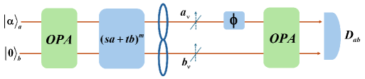
Figure 1: Schematic diagram of D-PSO within the SU(1,1). OPA is the optical parametric amplifier, D-PSO act behind the first OPA. The symbol of $\phi$ is corresponding to the phase shifter, and $D_{ab}$ is the intensity detector between mode $a$ and mode $b$. The two fictitious BSs inside the SU (1,1) interferometer are used to describe the photon losses on the mode $a$ and mode $b$ , respectively.

The normalization constants can be calculated as:

$$A=\left(Q_{m,0,0,0,0}\right)^{-\frac{1}{2}}.$$ (2)

The specific derivation of $Q_{m,x_{1},y_{1},x_{2},y_{2}}$ is shown in Appendix A.

III Phase sensitivity

In phase estimation, different detection methods can lead to different effects on phase sensitivity. Selecting an appropriate detection method can measure phase changes more accurately and minimize errors. Commonly used detection methods are: intensity detection a16 ; a17 , homodyne detection a18 ; a19 , parity detection a20 ; a21 . Considering the accuracy and simplicity of intensity detection, in our scheme, we perform intensity detection on mode $a$ and $b$.

The photon-number sum operator of mode $a$ and mode $b$ is $X=a^{\dagger}a+b^{{\dagger}}b$, based on the error-propagation equation a8 , the phase sensitivity of the SU(1,1) interferometer can be given by the following formula:

$$\Delta\phi=\frac{\sqrt{\left\langle\Delta^{2}X\right\rangle}}{|\partial\left\langle X\right\rangle/\partial\phi|}=\frac{\sqrt{\left\langle X^{2}\right\rangle-\left\langle X\right\rangle^{2}}}{|\partial\left\langle X\right\rangle/\partial\phi|},$$ (3)

where $\langle X\rangle=\left\langle\Psi_{out}\right|(a^{\dagger}a+b^{{\dagger}}b)\left|\Psi_{out}\right\rangle$. Detailed calculation steps for the phase sensitivity $\Delta\phi$ of the D-PSO are provided in Appendix A.

First, we consider the effects of different parameters on the phase sensitivity without photon loss. We take the influence of the order $m$ on the phase sensitivity into account, where $T=1$ representing the scenario without photon losses. We fix $\alpha=1$, $g=1$ and the optimal phase sensitivity is obtained by optimizing the coefficient $t$ of the D-PSO. We compare the influences of without non-Gaussian operation, L-PSO and D-PSO on the phase sensitivity respectively in Fig. 2. It is shown that, (i) when there is no non-Gaussian operation, the phase sensitivity $\Delta\phi$ first improves and then weakens with the increase of phase shift $\varphi\$and the phase sensitivity reaches its optimal value $\Delta\phi\approx 0.25$ when $\left|\varphi\right|\approx 0.7$. (The smaller the phase sensitivity is, the higher the precision is.) (ii) In the presence of L-PSO, the variation trend of phase sensitivity $\Delta\phi$ with phase shift $\varphi$ is the same as described above. Notably, the value of the optimal phase sensitivity $(\Delta\phi\approx 0.18)$ outperforms that in the previous case, while the absolute value of the corresponding phase shift is larger. That is, the value of $\varphi$ corresponding to the optimal point shifts toward larger values of $\varphi$. Additionally, the phase sensitivity of mode $b$ is superior to that of mode $a$. (iii) It is interesting that, the optimal range of phase shift $\varphi$ in D-PSO can encompass the optimal ranges of both modes $a$ and $b$, which means that the D-PSO is able to combine advantages of the L-PSO. And in almost the entire space of $\varphi$, D-PSO demonstrates the best performance compared with the original operation and the L-PSO scheme. (iv) As the order $m$ increases, the optimal phase sensitivities $\Delta\phi$ of the two L-PSOs gradually improve, and the difference in their corresponding phase shifts $\varphi$ gradually increases. (Combined with the Fig. 2, the phase sensitivity $\Delta\phi$ reaches its optimum when $\varphi$ is approximately equal to 1. So in order to facilitate comparison, we take $\varphi=1$ in the subsequent images.) (v) Compared with the standard case, both L-PSO and D-PSO can improve the phase sensitivity and D-PSO has a better improvement effect than L-PSO. Therefore, in the following sections, we will only focus on the comparison between L-PSO and D-PSO.

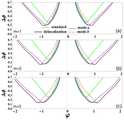
Figure 2: The comparison between D-PSO and L-PSO, about phase sensitivity $\Delta\phi$ as a function of $\varphi$, with $\alpha=1$, $g=1\$and$\ T=1$. Standard represents the standard SU(1,1) interferometer (without non-Gaussian operations). Mode $a$ represents the photon subtraction operation only performed on mode $a$ $(s=1,t=0)$, mode $b$ represents the photon subtraction operation only performed on mode $b$ $(s=0,t=1)$ and delocalization means D-PSO.

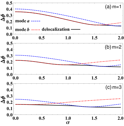
Figure 3: The comparison between D-PSO and L-PSO, about phase sensitivity $\Delta\phi$ as a function of coherent amplitude $\alpha$, with $\varphi=1$, $g=1\$and$\ T=1$.

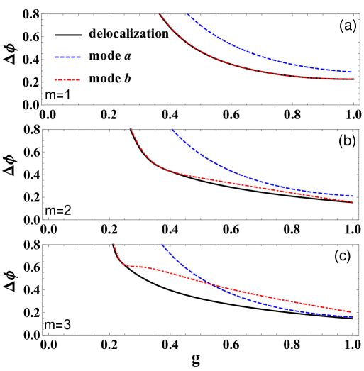
Figure 4: The comparison between D-PSO and L-PSO, about phase sensitivity $\Delta\phi$ as a function of gain factor $g$, with $\varphi=1$, $\alpha=1\$and$\ T=1$.

Next, we further investigate the influence of other parameters on the phase sensitivity in ideal case. The phase sensitivity $\Delta\phi$ is plotted in Fig. 3 as a function of coherent amplitude $\alpha$. By comparing the effects of L-PSO and D-PSO, it is interesting to notice that, (i) with the increasing of coherent amplitude $\alpha$, phase sensitivity $\Delta\phi$ gardually improves and then decreases when L-PSO are applied. And when $\alpha<1.75$ and $m=1$, the phase sensitivity $\Delta\phi$ of mode $b$ is greater than that of mode $a$. But as $m$ increases, the range of $\alpha$ for which mode $b$ outperforms mode $a$ will gradually decrease. Besides, the coherent amplitude $\alpha$ value corresponding to the optimal phase sensitivity $\Delta\phi$ of mode $a$ $(\alpha\approx 1.5)\$is bigger than that of mode $b$ $(\alpha\approx 1.9)$ and the difference in coherent amplitudes between the two L-PSOs increases with the order $m$ grows. (ii) The phase sensitivity $\Delta\phi$ of the D-PSO operation can encompass the optimal phase sensitivity $\Delta\phi$ of the L-PSO operation and it always maintains a low trend almost without rising. So when the value of the order $m$ increases, the range of coherent amplitude $\alpha$ within which the phase sensitivity of D-PSO outperforms that of L-PSO gradually expands.

Fig. 4 shows the curve of how the phase sensitivity $\Delta\phi$ varies with gain factor $g$. We find that, (i) the phase sensitivity $\Delta\phi$ improves as gain factor$\ g$ increases under the condition of L-PSO. (ii) The phase sensitivity $\Delta\phi$ of mode $b$ is generally superior to that of mode $a$, but this trend undergoes a change when $m=3$ and $g>0.55$. (iii) D-PSO can encompass the optimal phase sensitivities in the two L-PSOs, and when there is an increase in the order $m$, the advantages of D-PSO over L-PSO in terms of phase sensitivity gradually emerge.

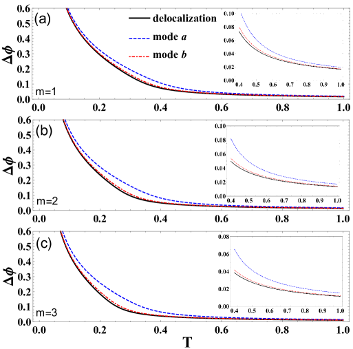
Figure 5: The comparison between D-PSO and L-PSO, about phase sensitivity $\Delta\phi$ as a function of $T$, with $\varphi=1$, $g=1\$and$\ \alpha=3$.

Since there exists loss in practical situations, now we consider the phase sensitivity $\Delta\phi$ in the case of loss. Here, $T$ is the transmissivity of the two fictitious BSs, and $T=1$ and $T=0$ represent the ideal and completely lossy cases. It is found from Fig. 4 as follows, (i) in most of the $T$ range ( $T$ is in the range of 0.4 to 1), both L-PSO and D-PSO show little variation with $T$, indicating that the two schemes are less affected by loss. Additionally, the sensitivity of mode $b$ in L-PSO outperforms that of mode $a$, and an increase in the order $m$ results in improved sensitivity. (ii) Throughout the entire $T$ range, the sensitivity of D-PSO is better than that of L-PSO, indicating that D-PSO exhibits stronger robustness against photon loss over a wide range.

IV
QFI and some theoretical limits

IV.1 QFI in ideal case

One of the popular ways to obtain useful bounds in quantum metrology, without the need for cumbersome optimization, is to use the concept of the QFI, which represents the maximum information extracted from the interferometer system a22 .

For a pure-state system, the QFI can be derived by a23

$$F=4\left[\left\langle\Psi_{\phi}^{\prime}|\Psi_{\phi}^{\prime}\right\rangle-\left|\left\langle\Psi_{\phi}^{\prime}|\Psi_{\phi}\right\rangle\right|^{2}\right],$$ (4)

where $\left|\Psi_{\phi}\right\rangle$ is the quantum state after the phase shift and before the second OPA and $\left|\Psi_{\phi}^{\prime}\right\rangle=\partial\left|\Psi_{\phi}\right\rangle/\partial\phi$. Then the QFI can be rewritten as a23 :

$$F=4\left\langle\Delta^{2}n_{a}\right\rangle,$$ (5)

where $\left\langle\Delta^{2}n_{a}\right\rangle=\left\langle\Psi_{\phi}\right|(a^{\dagger}a)^{2}|\Psi_{\phi}\rangle-(\left\langle\Psi_{\phi}\right|a^{\dagger}a|\Psi_{\phi}\rangle)^{2}$.

In our scheme, the quantum state is given by:

$$\left|\Psi_{\phi}\right\rangle=AU_{\phi}\left(sa+tb\right)^{m}U_{S_{1}}|\psi_{in}\rangle,\mathit{\ }$$ (6)

where $|\psi_{in}\rangle=\left|\alpha\right\rangle_{a}\otimes\left|0\right\rangle_{b}$. Thus, the QFI is derived as:

$$F=4\left[A^{2}\left(Q_{2,2,0,0}+Q_{1,1,0,0}\right)-(A^{2}Q_{1,1,0,0})^{2}\right].$$ (7)

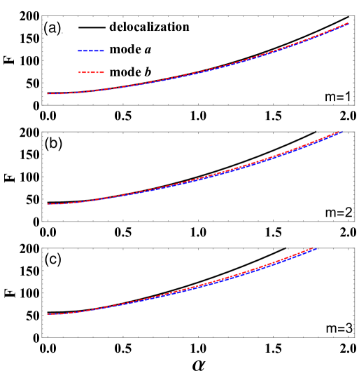
Figure 6: The comparison between D-PSO and L-PSO, on QFI as a function of $\alpha$, with $\varphi=1$, $g=1\$and$\ T=1$.

In order to investigate how the QFI varies with the parameters, we plot the curves of the QFI as a function of coherent amplitude $\alpha$ and gain factor$\ g$. In Fig. 6, it is clear to see that, (i) under a given $m$, with the increasing of coherent amplitude $\alpha$, the QFI of both D-PSO and L-PSO will enlarge. (ii) Compared to the L-PSO, the QFI of D-PSO will be larger when the value of $\alpha$ is greater than 1 ($m=1$), which will be more obvious as the order $m$ grows.

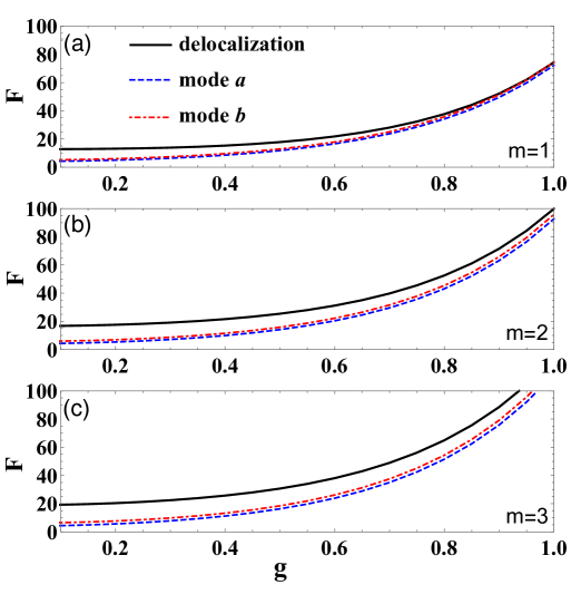
Figure 7: The comparison between D-PSO and L-PSO, on QFI as a function of $g$, with $\varphi=1$, $\alpha=1\$and$\ T=1$.

Fig. 7 shows that the QFI as a function of $g$, with $\alpha=1$, $T=1$. We notice that, (i) the QFI goes up as gain factor $g$ gets larger. (ii) When the order $m$ is the same, it is clearly found that the QFI of D-PSO is greater than that of L-PSO. (iii) As the order $m$ increases, the difference of QFI between the two L-PSOs becomes more pronounced, and the discrepancy in QFI between the D-PSO and L-PSO also becomes more evident.

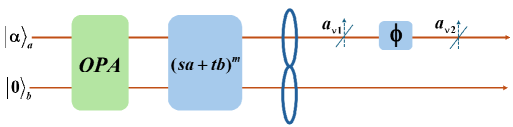
Figure 8: The calculation model of the Fisher information under losses. The loss occurs on the mode $a$.

IV.2
QFI in lossy case

In practical situations, the influence of photon loss on the phase estimation cannot be neglected. The QFI calculation model under loss condition is shown in Fig. 8. The small phase shift occurs in mode $a$ inside the SU(1,1) interferometer. For simplicity, we only consider the photon loss in mode $a$. The method of calculating the QFI in the presence of photon loss is proposed by Escher et al. a23 , which can be briefly summarized in the following: for an arbitrary initial pure state $\left|\Psi_{s}\right\rangle$, in the probe system S, the QFI with photon loss can be calculated as:

$$F_{L}=\min C_{Q}\left[\left|\psi_{S}\right\rangle,\Pi_{l}\left(\phi\right)\right],$$ (8)

where $\Pi_{l}\left(\phi\right)$ is the Kraus operator which acts on the system S and describes the photon loss, and $C_{Q}\left[\left|\psi_{S}\right\rangle,\Pi_{l}\left(\phi\right)\right]$, can be further calculated as:

$$C_{Q}\left[\left|\psi_{S}\right\rangle,\Pi_{l}\left(\phi\right)\right]=4[\left\langle\Psi\right|H_{1}\left|\Psi\right\rangle-\left|\left\langle\Psi\right|H_{2}\left|\Psi\right\rangle\right|^{2}],$$ (9)

where $\left|\Psi\right\rangle$ is the state before loss and after the first non-Gaussian operation, and$\ H_{1}$ and $H_{2}$ are defined as:

$$H_{1} = \overset{\infty}{\underset{l}{\sum}}\frac{d\Pi_{l}^{{\dagger}}\left(\phi,\eta,\lambda\right)}{d\phi}\frac{d\Pi_{l}\left(\phi,\eta,\lambda\right)}{d\phi},$$ (10)

$$H_{2} = \overset{\infty}{\underset{l}{i\sum}}\frac{d\Pi_{l}^{{\dagger}}\left(\phi,\eta,\lambda\right)}{d\phi}\Pi_{l}\left(\phi,\eta,\lambda\right).$$ (11)

The Kraus operation $\Pi_{l}\left(\phi,\eta,\lambda\right)$ can be chosen as:

$$\Pi_{l}\left(\phi,\eta,\lambda\right)=\sqrt{\frac{\left(1-\eta\right)^{l}}{l!}}e^{i\phi\left(n-\lambda l\right)}\eta^{\frac{n}{2}}a^{l},$$ (12)

where $n$ is the photon number operator, $\lambda=0$ and $\lambda=-1$ represent that the loss occur before and after the phase shift, respectively. $\eta\$quantifies the photon loss, where $\eta=1\$and $\eta=0\$represent the situations of complete lossy and absorption. The parameters $\Pi_{l}\left(\phi,\eta,\lambda\right)$ defines a set of Kraus operators, which are used to minimize the value of $C_{Q}$. In our model, the Fisher information under lossy case can be calculated as a23

$$F_{L}=\frac{4\eta\langle n\rangle\langle\Delta n^{2}\rangle}{\left(1-\eta\right)\langle\Delta n^{2}\rangle+\eta\langle n\rangle},$$ (13)

where $\langle n\rangle$ and $\langle\Delta n^{2}\rangle\$are the total average photon number and the variance of the total average photon number of mode $a$ inside the SU(1,1) interferometer. And it can be calculated as:

$$\langle n\rangle=A^{2}\left\langle\Psi\right|n_{a}\left|\Psi\right\rangle=A^{2}Q_{m,1,1,0,0},$$ (14)

and

$$\langle\Delta n^{2}\rangle = A^{2}\left\langle\Psi\right|n_{a}^{2}\left|\Psi\right\rangle-\langle n\rangle$$ (15)

$$= 4[A^{2}\left(Q_{m,2,2,0,0}+Q_{m,1,1,0,0}\right)$$

$$-\left(A^{2}Q_{m,1,1,0,0}\right)^{2}].$$

In the presence of photon loss, we analyze the influence of each parameter on the QFI. By observing the QFI varying with $\eta\$and$\ \alpha\$shown in Fig. 9 and Fig. 10, it is clear to see that, (i) with the increasing of $\eta\$and $\alpha$, QFI will become higher. (ii) Compared with the L-PSO, the QFI of the D-PSO under lossy case can cover the advantages of L-PSO and it even exceeds L-PSO when $m=1$, $\eta\ >0.6$ and $\alpha>1.2$. This trend will gradually become more obvious as order $m$, $\eta\$ and  $\alpha\$increases.

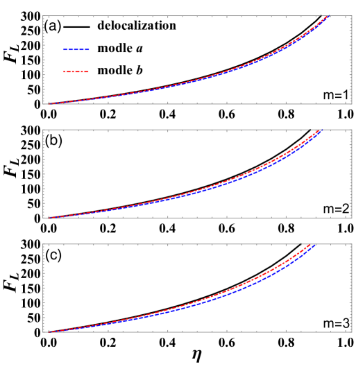
Figure 9: The comparison between D-PSO and L-PSO, on $F_{L}$ as a function of $\eta$, with $g=1$, $\alpha=3$.

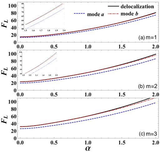
Figure 10: The comparison between D-PSO and L-PSO, on $F_{L}$ as a function of $\alpha$, with $g=1$, $T=0.7$.

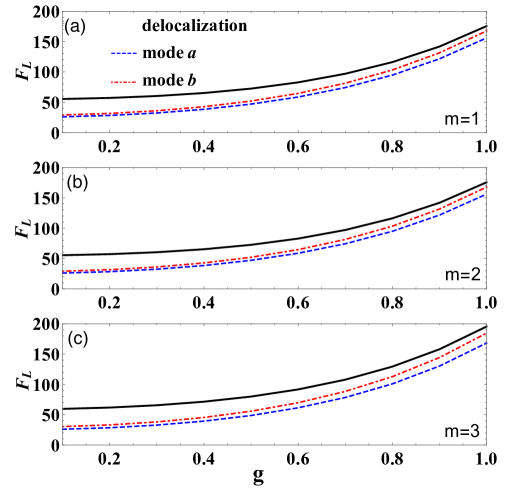
Figure 11: The comparison between D-PSO and L-PSO, on $F_{L}$ as a function of $g$, with $\alpha=1$, $T=0.7$.

By observing the changes of the QFI with gain factor $g$ shown in Fig. 11, it can be seen that, (i) the QFI in loss gradually increases with the increase of the gain factor $g$. (ii) The QFI of L-PSO in mode $b$ in lossy case exceeds that in mode $a$, and D-PSO can combine the advantages of both L-PSO operations across the entire range of $g\$and significantly outperform their QFI. (iii) The trend that D-PSO is superior to L-PSO increases with the increase of the order $m$, and the QFI differerence becomes smaller as gain $g$.

IV.3 Comparison phase sensitivities and theoretical limits

In this subsection, we compare the phase sensitivity with some theoretical limits, including the QCRB, the SQL, and the HL. The QCRB is often used to determine the ultimate phase precision of an interferometer and can be derived by the QFI a24 . Therefore, in our scheme, the QCRB in ideal case is given by:

$$\Delta\phi_{QCRB}=\frac{1}{\sqrt{vF}},$$ (16)

where $v$ represents the number of measurements. For simplicity, we set $v=1$. The SQL and HL are defined as: $\Delta\phi_{SQL}=1/\sqrt{N}$ and $\Delta\phi_{HL}=1/N$, where $N$ represent the total average photon number inside the interferometer and before the second OPA. $N$ can be calculated as:

$$N = \left\langle\Psi_{\phi}\right|\left(a^{{\dagger}}a+b^{{\dagger}}b\right)|\Psi_{\phi}\rangle$$ (17)

$$= A^{2}(Q_{1,1,0,0}+Q_{0,0,1,1}).$$

Figs. 12 and 13 show the comparison of the phase sensitivity $\Delta\phi$ for L-PSO and D-PSO with the SQL, the HL and the QCRB when $m=1$, $m=2$ and $m=3$ respectively, under the condition of $T=1$ and $T=0.7$. We can find in Fig. 12, (i) as the order $m$ increases, the D-PSO can break through the SQL, and it even can exceed the HL when $m>1\$and $\alpha<1$. (ii) The phase sensitivity of the D-PSO can get close to the QCRB when the order $m$ increases and is closer than that of the L-PSO. It’s interesting to find from Fig. 13 that, in a lossy case, (i) the D-PSO can still break through the SQL, and exceed the HL when $m=1$ and $\alpha<0.3$. This trend will be more obvious as the order $m$ grows. A comparison between Fig. 12 and Fig. 13 shows that both D-PSO and L-PSO are robust against internal loss. However, when the order $m$ and coherent amplitude $\alpha$ increase, D-PSO outperforms L-PSO.

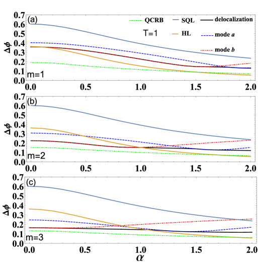
Figure 12: The comparison of the phase sensitivity $\Delta\phi$  in D-PSO and L-PSO with the SQL, the HL, and the QCRB, where gain factor $g=1$, $\varphi=1\$and $T=1$.

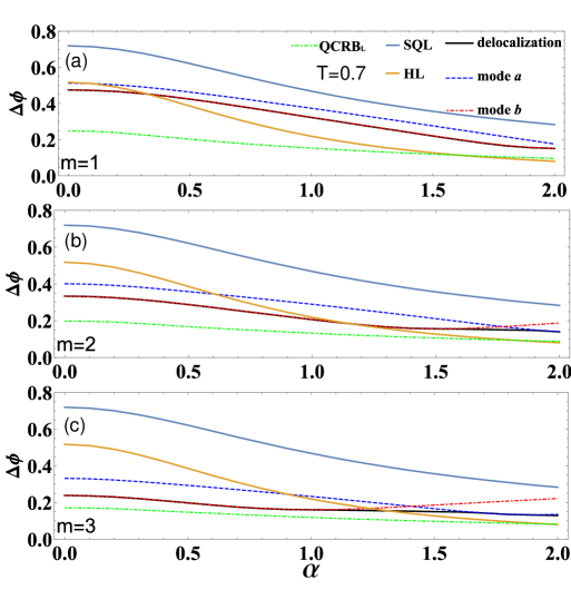
Figure 13: The comparison of the phase sensitivity $\Delta\phi$  in D-PSO and L-PSO with the SQL, the HL, and the QCRB, where gain factor $g=1$, $\varphi=1\$and $T=0.7$.

V Conclusion

In this paper, we have studied the effects of implementing the D-PSO inside the SU(1,1) interferometer on the phase sensitivity and QFI under both the ideal and the photon-loss conditions. In addition, we have also studied the effects of the gain coefficient $g$ of the OPA, the coherent amplitude $\alpha$, and the transmittance $T$ of the BS on the performance of the system. Through analysis and comparison, we have verified that the D-PSO can improve the measurement accuracy of the SU(1,1) interferometer and enhance its robustness against internal photon loss. In addition, we also compared the differences between the D-PSO and the L-PSO. In terms of phase sensitivity, after optimization, the optimal range of phase shift $\varphi$, the coherent amplitude $\alpha$, the gain coefficient $g\$and the transmittance $T\$in D-PSO can encompass the optimal ranges of both mode $a$ and mode $b$, which means that the D-PSO is able to combine and exceed the advantages of the L-PSO. In terms of QFI, regardless of whether it is in an ideal or realistic situation, compared with the L-PSO, the QFI of the D-PSO will be larger under certain circumstances. Furthermore, as the order $m$ increases, the phase sensitivity of the D-PSO can get closer to the QCRB and has a stronger ability to resist internal loss. Our results are hoped to find important applications in quantum metrology and quantum information.

APPENDIX A : THE CALCULATION OF THE PHASE SENSITIVITY FOR THE D-PSO

In this Appendix, we give the derivation of the phase sensitivity $\Delta\phi$. In our scheme, the transform relation between the output state $\left|\Psi_{out}\right\rangle$ and the input state $\left|\Psi_{in}\right\rangle$is given by:

$$\left|\Psi_{out}\right\rangle=AU_{S_{2}}U_{\phi}U_{B}\left(sa+tb\right)^{m}U_{S_{1}}\left|\Psi_{in}\right\rangle.$$ (A1)

Before deriving the phase sensitivity (Eq. (3)), we introduce a formula, i.e.,

$$Q_{m,x_{1},y_{1},x_{2},y_{2}}$$

$$=\left\langle\Psi_{in}\right|U_{S_{1}}^{\dagger}\left(sa^{\dagger}+tb^{\dagger}\right)^{m}U_{B}^{\dagger}\times\left(a^{\dagger x_{1}}a^{y_{1}}b^{\dagger x_{2}}b^{y_{2}}\right)$$

$$\times U_{B}\left(sa+tb\right)^{m}U_{S_{1}}\left|\Psi_{in}\right\rangle$$

$$=\frac{\partial^{2m+x_{1}+y_{1}+x_{2}+y_{2}}}{\partial\lambda_{3}^{m}\partial\lambda_{4}^{m}\partial\lambda_{5}^{x_{1}}\partial\lambda_{6}^{y_{1}}\partial\lambda_{7}^{x_{2}}\partial\lambda_{8}^{y_{2}}}$$

$$\times U_{S_{1}}^{\dagger}e^{\lambda_{3}s^{\ast}a^{{\dagger}}}e^{\lambda_{3}t^{\ast}b^{{\dagger}}}U_{B}^{\dagger}e^{\lambda_{5}a^{{\dagger}}}e^{\lambda_{6}a}e^{\lambda_{7}b^{{\dagger}}}e^{\lambda_{8}b}U_{B}$$

$$\times e^{s\lambda_{4}a}e^{\lambda_{4}tb}U_{S1}|_{\lambda_{3}=\lambda_{4}=\lambda_{5}=\lambda_{6}=\lambda_{7}=\lambda_{8}=0}$$

$$=\frac{\partial^{2m+x_{1}+y_{1}+x_{2}+y_{2}}}{\partial\lambda_{3}^{m}\partial\lambda_{4}^{m}\partial\lambda_{5}^{x_{1}}\partial\lambda_{6}^{y_{1}}\partial\lambda_{7}^{x_{2}}\partial\lambda_{8}^{y_{2}}}$$

$$\times\left\{\exp\left[w_{4}\right]\right\}_{{}_{\lambda_{3}=\lambda_{4}=\lambda_{5}=\lambda_{6}=\lambda_{7}=\lambda_{8}=0,}}$$ (A2)

where

$$w_{1} =-(\lambda_{8}\sqrt{T}+\lambda_{4}t)\sinh g$$

$$\times[(\lambda_{6}\sqrt{T}+\lambda_{4}s)\cosh g$$

$$-(\lambda_{7}\sqrt{T}+\lambda_{3})\sinh g]$$

$$-(\lambda_{5}\sqrt{T}+\lambda_{3})\sinh g$$

$$\times[(\lambda_{7}\sqrt{T}+\lambda_{3})\cosh g$$

$$-(\lambda_{6}\sqrt{T}+\lambda_{4}s)\sinh g],$$ (A3)

$$w_{2} =(\lambda_{5}\sqrt{T}+\lambda_{3})\cosh g$$

$$-(\lambda_{8}\sqrt{T}+\lambda_{4}t)\sinh g,$$ (A4)

$$w_{3} =(\lambda_{6}\sqrt{T}+\lambda_{4}s)\cosh g$$

$$-(\lambda_{7}\sqrt{T}+\lambda_{3})\sinh g,$$ (A5)

$$w_{4}=w_{1}+w_{2}\alpha^{\ast}+w_{3}\alpha.$$ (A6)

Here $m$, $x_{1}$, $x_{2}$, $y_{1}$, $y_{2}$ are positive integers, $\lambda_{3}$, $\lambda_{4}$, $\lambda_{5}$, $\lambda_{6}$, $\lambda_{7}$, $\lambda_{8}$ are differential variables. After differentiation, all these differential variables take zero.

In order to derive Eq. (3), we use the transformation relations, i.e.

$$U_{S1}^{\dagger}aU_{S1} =a\cosh g-b^{\dagger}e^{i\theta_{1}}\sinh g,\$$

$$U_{S1}^{\dagger}bU_{S1} =b\cosh g-a^{\dagger}e^{i\theta_{1}}\sinh g,\$$ (A7)

$$U_{S_{2}}^{\dagger}aU_{S2} =a\cosh g-b^{\dagger}e^{i\theta_{2}}\sinh g,$$

$$U_{S2}^{\dagger}bU_{S2} =b\cosh g-a^{\dagger}e^{i\theta_{2}}\sinh g,\$$ (A8)

$$U_{B}^{\dagger}aU_{B} =\sqrt{T}a+\sqrt{R}a_{\nu},$$

$$U_{B}^{\dagger}a^{\dagger}U_{B} =\sqrt{T}a^{\dagger}+\sqrt{R}a_{\nu}^{\dagger},$$ (A9)

$$U_{B}^{\dagger}bU_{B} =\sqrt{T}b+\sqrt{R}b_{v},$$

$$U_{B}^{\dagger}b^{{\dagger}}U_{B} =\sqrt{T}b^{{\dagger}}+\sqrt{R}b_{v}^{{\dagger}}.$$ (A10)

In our scheme, the phase sensitivity can be calculated as:

$$\Delta\phi=\frac{\sqrt{\begin{array}[]{c}\left\langle\Psi_{out}\right|\left(a^{\dagger}a+b^{{\dagger}}b\right)^{2}\left|\Psi_{out}\right\rangle\\ -\left\langle\Psi_{out}\right|\left(a^{\dagger}a+b^{{\dagger}}b\right)\left|\Psi_{out}\right\rangle^{2}\end{array}}}{|\partial\left\langle\Psi_{out}\right|\left(a^{\dagger}a+b^{{\dagger}}b\right)\left|\Psi_{out}\right\rangle/\partial\phi|},$$ (A11)

where

$$\left\langle\Psi_{out}\right|\left(a^{\dagger}a+b^{{\dagger}}b\right)^{2}\left|\Psi_{out}\right\rangle$$

$$=\left\langle\Psi_{out}\right|\left(a^{\dagger 2}a^{2}\right)\left|\Psi_{out}\right\rangle+\left\langle\Psi_{out}\right|\left(a^{\dagger}a\right)\left|\Psi_{out}\right\rangle$$

$$+2\left\langle\Psi_{out}\right|\left(a^{\dagger}ab^{{\dagger}}b\right)\left|\Psi_{out}\right\rangle$$

$$+\left\langle\Psi_{out}\right|\left(b^{\dagger 2}b^{2}\right)\left|\Psi_{out}\right\rangle+\left\langle\Psi_{out}\right|\left(b^{\dagger}b\right)\left|\Psi_{out}\right\rangle,$$ (A12)

and

$$\left\langle\Psi_{out}\right|\left(a^{\dagger 2}a^{2}\right)\left|\Psi_{out}\right\rangle$$

$$=\cosh^{4}gQ_{m,2,2,0,0}+2e^{-i\phi}\sinh g\cosh^{3}gQ_{m,2,1,1,0}$$

$$+e^{-2i\phi}\sinh^{2}g\cosh^{2}gQ_{m,2,0,2,0}$$

$$+2e^{i\phi}\sinh g\cosh^{3}gQ_{m,1,2,0,1}$$

$$+4\sinh^{2}g\cosh^{2}g\left(Q_{m,1,1,1,1}+Q_{m,1,1,0,0}\right)$$

$$+2e^{-i\phi}\sinh^{3}g\cosh g\left(Q_{m,1,0,2,1}+2Q_{m,1,0,1,0}\right)$$

$$+e^{2i\phi}\sinh^{2}g\cosh^{2}gQ_{m,0,2,0,2}$$

$$+2e^{i\phi}\sinh^{3}g\cosh g\left(Q_{m,0,1,1,2}+2Q_{m,0,1,0,1}\right)$$

$$+\sinh^{4}g\left(Q_{m,0,0,2,2}+4Q_{m,0,0,1,1}\right)$$

$$+2\sinh^{4}gQ_{m,0,0,0,0},$$ (A13)

$$\left\langle\Psi_{out}\right|\left(a^{\dagger}a\right)\left|\Psi_{out}\right\rangle$$

$$=\cosh^{2}gQ_{m,1,1,0,0}+e^{-i\phi}\sinh g\cosh gQ_{m,1,0,1,0}$$

$$+e^{i\phi}\sinh g\cosh gQ_{m,0,1,0,1}$$

$$+\left(Q_{m,0,0,1,1}+Q_{m,0,0,0,0}\right)\sinh^{2}g,$$ (A14)

and

$$\left\langle\Psi_{out}\right|\left(b^{\dagger 2}b^{2}\right)\left|\Psi_{out}\right\rangle$$

$$=\cosh^{4}gQ_{m,0,0,2,2}+2e^{-i\phi}\sinh g\cosh^{3}gQ_{m,1,0,2,1}$$

$$+e^{-2i\phi}\sinh^{2}g\cosh^{2}gQ_{m,2,0,2,0}$$

$$+2e^{i\phi}\sinh g\cosh^{3}gQ_{m,0,1,1,2}$$

$$+4\sinh^{2}g\cosh^{2}g\left(Q_{m,1,1,1,1}+Q_{m,0,0,1,1}\right)$$

$$+2e^{-i\phi}\sinh^{3}g\cosh g\left(Q_{m,2,1,1,0}+2Q_{m,1,0,1,0}\right)$$

$$+e^{2i\phi}\sinh^{2}g\cosh^{2}gQ_{m,0,2,0,2}$$

$$+2e^{i\phi}\sinh^{3}g\cosh g\left(Q_{m,1,2,0,1}+2Q_{m,0,1,0,1}\right)$$

$$+\sinh^{4}g\left(Q_{m,2,2,0,0}+4Q_{m,1,1,0,0}\right)$$

$$+2\sinh^{4}gQ_{m,0,0,0,0},$$ (A15)

$$\left\langle\Psi_{out}\right|\left(b^{\dagger}b\right)\left|\Psi_{out}\right\rangle$$

$$=\cosh^{2}gQ_{m,0,0,1,1}+e^{-i\phi}\sinh g\cosh gQ_{m,1,0,1,0}$$

$$+e^{i\phi}\sinh g\cosh gQ_{m,0,1,0,1}$$

$$+\sinh^{2}gQ_{m,1,1,0,0}+\sinh^{2}gQ_{m,0,0,0,0}.$$ (A16)

References

- (1) Giovannetti, V., Lloyd, S. & Maccone, L. Advances in quantum metrology. Nature Photon 5, 222–229 (2011).
- (2) Gregory Krueper, Lior Cohen, and Juliet T. Gopinath, Cascaded multiparameter quantum metrology, Phys. Rev. A. 111, 012618 (2025).
- (3) S. Pang and A. N. Jordan, Optimal adaptive control for quantum metrology with time-dependent Hamiltonians, Nat. Commun. 8, 14695 (2017).
- (4) W. Ge, K. Jacobs, Z. Eldredge, A. V. Gorshkov, and M. Foss-Feig, Distributed Quantum Metrology with Linear Networks and Separable Inputs, Phys. Rev. Lett. 121, 043604 (2018).
- (5) S. M. Roy and S. L. Braunstein, Exponentially enhanced quantum metrology, Phys. Rev. Lett. 100, 220501 (2008).
- (6) T. Corbitt and N. Mavalvala, Quantum noise in gravitational-wave interferometers, Journal of optics. B, S675–S683 (2004).
- (7) R. X. Adhikari, Gravitational radiation detection with laser interferometry, Rev. Mod. Phys. 86, 121 (2014).
- (8) E. Oelker, L. Barsotti, S. Dwyer, D. Sigg, and N. Mavalvala, Squeezed light for advanced gravitational wave detectors and beyond, Opt. Express, 22, 21106–21121 (2014).
- (9) H.Vahlbruch, D. Wilken, M. Mehmet, and B. Willke, Laser power stabilization beyond the shot noise limit using squeezed light, Phys. Rev. L. 121, 173601 (2018).
- (10) P. Gill, Atomic clocks- raising the standards, Sci. 294, 1666–1668 (2001).
- (11) S. Weinberg, Lindblad decoherence in atomic clocks, Phys. Rev. A. 94, 042117 (2016).
- (12) M. Arndt and C. Brand, Interference of atomic clocks, Sci. 349, 1168–1169 (2015).
- (13) Andrew D. Ludlow, Martin M. Boyd, Jun Ye, E. Peik, and P. O. Schmidt, Optical atomic clocks, Rev. Mod. Phys. 87, 637 (2015).
- (14) N. Bornman, S. Prabhakar, A. Valles, J. Leach, and A. Forbes, Ghost imaging with engineered quantum states by hong-ou-mandel interference, New J. Phys 21, 073044 (2019).
- (15) M. Tsang, Quantum imaging beyond the diffraction limit by optical centroid measurements, Phys. Rev. L. 102, 253601 (2009).
- (16) C. Thiel, T. Bastin, J. Martin, E. Solano, J. von Zanthier, and G. S. Agarwal, Quantum imaging with incoherent photons, Phys. Rev. L. 99, 133603 (2007).
- (17) A. Mikhalychev, S. Almazrouei, S. Mikhalycheva, A. Bouchalkha, D. Mogilevtsev, and B. Ahmedov, Efficient estimation of error bounds for quantum multiparametric imaging with constraints, Phys. Rev. A. 111, 032618 (2025).
- (18) S. D. Huver, C. F. Wildfeuer, and J. P. Dowling, Entangled fock states for robust quantum optical metrology, imaging, and sensing, Phys. Rev. A. 78, 063828 (2008).
- (19) Jianxin Chen, Toby S. Cubitt, Aram W. Harrow, and Graeme Smith, Entanglement can Completely Defeat Quantum Noise, Phys. Rev. Lett. 107, 250504 (2011).
- (20) C. M. Caves, Quantum-mechanical noise in an interferometer, Phys. Rev. D 23, 1693 (1981).
- (21) Dowling, J. P. Quantum optical metrology – the lowdown on high-N00N states. Contemporary Physics, 49(2), 125–143 (2008).
- (22) T. Kim, J. Shin, Y. Ha, H. Kim, G. Park, T. G. Noh, and C. K. Hong, The phase-sensitivity of a Mach–Zehnder interferometer for Fock state inputs, Opt. Commun. 156, 37 (1998).
- (23) Luca Pezzé and Augusto Smerzi, Ultrasensitive Two-Mode Interferometry with Single-Mode Number Squeezing, Phys. Rev. Lett. 110, 163604 (2013).
- (24) Luca Pezzé and Augusto Smerzi, Mach-Zehnder Interferometry at the Heisenberg Limit with Coherent and Squeezed-Vacuum Light, Phys. Rev. Lett. 100, 073601 (2008).
- (25) Stefan Ataman, Optimal Mach-Zehnder phase sensitivity with Gaussian states, Phys. Rev. A. 100, 063821 (2019).
- (26) Karunesh K. Mishra, and Stefan Ataman, Optimal phase sensitivity of an unbalanced Mach-Zehnder interferometer, Phys. Rev. A. 106, 023716 (2022).
- (27) Zekun Zhao, Qingqian Kang, Huan Zhang, Teng Zhao, Cunjin Liu, and Liyun Hu, Phase estimation via coherent and photon-catalyzed squeezed vacuum states, Opt. Express 32, 28267 (2024).
- (28) B. Yurke, S. L. McCall, and J. R. Klauder, SU (2) and SU (1,1) interferometers, Phys. Rev. A 33(6), 4033–4054 (1986).
- (29) Jian-Dong Zhang, Chenglong You, Chuang Li, and Shuai Wang, Phase sensitivity approaching the quantum Cramér-Rao bound in a modified SU(1,1) interferometer, Phys. Rev. A. 103,032617 (2021).
- (30) Huan Zhang, Wei Ye, Chaoping Wei, Ying Xia, Shoukang Chang, Zeyang Liao, and Liyun Hu, Improved phase sensitivity in a quantum optical interferometer based on multiphoton catalytic two-mode squeezed vacuum states, Phys. Rev. A. 103, 013705 (2021).
- (31) Qingqian Kang, Zekun Zhao, Teng Zhao, Cunjin Liu, and Liyun Hu, Phase estimation via a number-conserving operation inside a SU(1,1) interferometer, Phys. Rev. A. 110, 022432 (2024).
- (32) Kun Zhang, Yinghui Lv, Yu Guo, Jietai Jing, and Wu-Ming Liu, Enhancing the precision of a phase measurement through phase-sensitive non-Gaussianity, Phys. Rev, A. 105, 042607 (2022).
- (33) Mattia Walschaers, Non-Gaussian Quantum States and Where to Find Them, PRX. Quantum. 2, 030204 (2021).
- (34) L. L. Guo, Y. F. Yu, and Z. M. Zhang, Improving the phase sensitivity of an SU(1,1) interferometer with photon-added squeezed vacuum light, Opt. Express 26, 29099 (2018).
- (35) Y. Ouyang, S. Wang, and L. J. Zhang, Quantum optical interferometry via the photon-added two-mode squeezed vacuum states, J. Opt. Soc. Am. B 33, 1373 (2016).
- (36) R. Birrittella and C. C. Gerry, Quantum optical interferometry via the mixing of coherent and photon-subtracted squeezed vacuum states of light, J. Opt. Soc. Am. B 31, 586 (2014).
- (37) Youke Xu, Teng Zhao, Qingqian Kang, Cunjin Liu, Liyun Hu, and Sanqiu Liu, Phase sensitivity of an SU(1,1) interferometer in photon-loss via photon operations, Opt. Express, 31, 8414 (2023).
- (38) S. K. Chang, W. Ye, H. Zhang, L. Y. Hu, J. H. Huang, and S. Q. Liu, Improvement of phase sensitivity in an SU(1,1) interferometer via a phase shift induced by a Kerr medium, Phys. Rev. A. 105, 033704 (2022).
- (39) Qingqing Sun, Hyunchul Nha, and M. Suhail Zubairy, Entanglement criteria and nonlocality for multimode continuous-variable systems, Phys. Rev. A. 80.020101 (2009).
- (40) Nicola Biagi, Luca S. Costanzo, Marco Bellini, and Alessandro Zavatta, Generating Discorrelated States for Quantum Information Protocols by Coherent Multimode Photon Addition, Adv. Quantum. Tech. 4, 2000141 (2021).
- (41) Nicola Biagi, Saverio Francesconi, Manuel Gessner, Marco Bellini, and Alessandro Zavatta, Remote Phase Sensing by Coherent Single Photon Addition, Adv. Quantum. Technol. 5, 2200039 (2022).
- (42) Nicola Biagi, Luca S. Costanzo, Marco Bellini, and Alessandro Zavatta, Entangling Macroscopic Light States by Delocalized Photon Addition, Phys. Rev. Lett. 124, 033604 (2020).
- (43) Stefan Ataman, Phase sensitivity of a Mach-Zehnder interferometer with single-intensity and difference-intensity detection, Phys. Rev. A. 98, 043856 (2018).
- (44) Shengshuai Liu, Yanbo Lou, Jun Xin, and Jietai Jing, Quantum Enhancement of Phase Sensitivity for the Bright-Seeded SU(1,1) Interferometer with Direct Intensity Detection, Phys. Rev. Applied. 10, 064046 (2018).
- (45) D. Li, C. H. Yuan, Z. Y. Ou, and W. Zhang, The phase sensitivity of an SU(1,1) interferometer with coherent and squeezed-vacuum light, New J. Phys. 16, 073020 (2014).
- (46) X. Y. Hu, C. P. Wei, Y. F. Yu, and Z. M. Zhang, Enhanced phase sensitivity of an SU(1,1) interferometer with displaced squeezed vacuum light, Front. Phys. 11, 114203 (2016).
- (47) P. M. Anisimov, G. M. Raterman, A. Chiruvelli, W. N. Plick, S. D. Huver, H. Lee, and J. P. Dowling, Quantum metrology with two-mode squeezed vacuum: Parity detection beats the Heisenberg limit, Phys.Rev.Lett. 104, 103602 (2010).
- (48) D. Li, B. T. Gard, Y. Gao, C. H. Yuan, W. Zhang, H. Lee, and J. P. Dowling, Phase sensitivity at the Heisenberg limit in an SU(1,1) interferometer via parity detection, Phys. Rev. A. 94, 063840 (2016).
- (49) Marcin Jarzyna and Rafał Demkowicz-Dobrzański, Quantum interferometry with and without an external phase reference, Phys. Rev. A. 85, 01180 (2012).
- (50) B. M. Escher, R. L. de Matos Filho, and L. Davidovich, General framework for estimating the ultimate precision limit in noisy quantum-enhanced metrology, Nat. Phys. 7, 406 (2011).
- (51) S. L. Braunstein and C. M. Caves, Statistical distance and the geometry of quantum states, Phys. Rev. Lett. 72(22), 3439–3443 (1994).