Spatial Correlation between Pulsars from Interfering Gravitational-Wave Sources in Massive Gravity

Abstract

In the nanohertz band, the spatial correlations in pulsar timing arrays (PTAs) produced by interfering gravitational waves (GWs) from multiple sources likely deviate from the traditional ones without interference under the assumption of an isotropic Gaussian ensemble. This work investigates the impact of such interference within the framework of massive gravity. Through simulations, we show that while the resulting correlation patterns can be described by Legendre expansions with coefficients that depend on the interference configuration, they remain predominantly quadrupolar ($l=2$), with this feature becoming more pronounced as the graviton mass increases—reflecting both the tensorial polarizations and the modified GW dispersion. However, the interference introduces significant variability in the angular correlation, making it difficult to distinguish massive gravity from general relativity based on a single realization of the Universe. We conclude that beyond a fundamental constraint set by the PTA observation time, achieving a substantially tighter bound on the graviton mass is statistically challenging and observationally limited under realistic conditions.

I Introduction

Whether the graviton has a non-zero mass remains one of the fundamental open questions in physics (Fierz and Pauli, 1939). Since the 1970s, significant theoretical efforts have been devoted to constructing a consistent and ghost-free theory of massive gravity van Dam and Veltman (1970); Zakharov (1970); Vainshtein (1972); Boulware and Deser (1972), leading to the development of prominent models such as the Dvali–Gabadadze–Porrati model Dvali and Gabadadze (2001); Dvali et al. (2000a, b) and the de Rham–Gabadadze–Tolley model de Rham et al. (2011). In parallel, extensive experimental and observational efforts have been made to detect or constrain the graviton mass—through, for example, tests of deviations from the Newtonian potential in the Solar System Bernus et al. (2020), observations of superradiant instabilities in supermassive black holes Brito et al. (2013), and measurements of weak gravitational lensing Choudhury et al. (2004). The advent of gravitational wave astronomy has opened a powerful new avenue for probing this question. Ground-based gravitational wave (GW) interferometers have placed bounds on the graviton mass using observed GW signals: the first detection, GW150914 Abbott et al. (2016) , yielded an upper limit of $m_{g}\leq 1.2\times 10^{-22}\mathrm{eV}/c^{2}$, which was subsequently improved to $m_{g}\leq 1.27\times 10^{-23}\mathrm{eV}/c^{2}$ using data from the Gravitational-Wave Transient Catalog (GWTC-3) Abbott et al. (2021).

In addition to ground-based detectors, pulsar timing arrays (PTAs) have also recently made significant progress in detecting the stochastic gravitational-wave background (SGWB). PTAs are sensitive to nanohertz signals by monitoring the times of arrival of radio pulses emitted from millisecond pulsars Sazhin (1978); Detweiler (1979); Foster and Backer (1990), where such signals induce differences between the expected and actual arrival times—known as timing residuals. In particular, the SGWB—whether of astrophysical or cosmological origin (Bi et al., 2023; Wu et al., 2024a)—generates timing residuals across different pulsars that exhibit a distinct spatial correlation Taylor et al. (2016); Burke-Spolaor et al. (2019). After decades of observation, the North American Nanohertz Observatory for Gravitational Waves (NANOGrav,  (Agazie et al., 2023a, b)), the European PTA (EPTA) in collaboration with the Indian PTA (InPTA) (Antoniadis et al., 2023a, b), the Parkes PTA (PPTA) (Zic et al., 2023; Reardon et al., 2023), and the Chinese PTA (CPTA) (Xu et al., 2023) have found evidence for a stochastic signal consistent with the Hellings-Downs (HD) correlation (Hellings and Downs, 1983), which is considered a smoking gun signature of the SGWB predicted by general relativity (GR). However, if the graviton possesses a nonvanishing mass, the dispersion relation of GWs would be modified, resulting in spatial correlations of timing residuals that deviate from the HD curve  (Lee et al., 2010; Liang and Trodden, 2021; Wu et al., 2023). These deviations open up the possibility of probing massive gravity using PTA data. Taking into account both this altered spatial correlation and the existence of a minimum frequency implied by a nonzero graviton mass, the NANOGrav 15-year data set places a tighter upper bound on the graviton mass than ground-based detectors, with $m_{g}\leq 8.2\times 10^{-24}\mathrm{eV}/c^{2}$ (Wu et al., 2024b).

Nevertheless, recent studies have highlighted that if the SGWB originates from supermassive black hole binaries, numerous sources in the nanohertz band emit gravitational waves at closely spaced frequencies, leading to interference effects (Roebber and Holder, 2017; Allen, 2023). Consequently, the actual spatial correlation may differ from the HD curve even within the framework of GR (Allen, 2023; Romano and Allen, 2024). While Ref. (Allen, 2023) interprets the HD curve as the ensemble average over an imaginary set of infinitely many independent Universes, where interference effects give rise to an irreducible variance in any single Universe, Ref. (Wu et al., 2024c) argues that, in our uniquely realized Universe, the spatial correlation is definite and determined by the specific interference scenario. However, the lack of access to detailed source information, such as phases and locations, results in a loss of predictability for the true correlation pattern. Ref. (Wu et al., 2024c) further analyzes the features of spatial correlation curves under various interference configurations, suggesting the possibility that the diversity of interference patterns could lead to degeneracies between the correlation expected in GR and those predicted by modified gravity theories. More critically, an SGWB originating from alternative theories would likewise exhibit interference effects, making it even more challenging to distinguish between competing theoretical models based on the observed correlation patterns.

In this work, we aim to investigate the spatial correlation patterns induced by realistic interference effects in the presence of a nonzero graviton mass, and to reassess the true discriminatory power of PTAs in testing massive gravity. We adopt natural units by setting the speed of light $c=1$ and the reduced Planck constant $\hbar=1$. The Earth is placed at the coordinate origin. Unit vectors are denoted by boldface symbols with hats, such as $\hat{\bm{\Omega}}$ and $\hat{\bm{p}}$. Latin subscripts are used with specific conventions throughout the paper: “$a$” and “$b$” denote abstract tensor indices; “$j$” and “$k$” label GW sources; and “A” and “B” label pulsars.

II Signal Correlations from Interfering Sources

For GW propagating in the direction $\hat{\bm{\Omega}}$, the four-wavevector in massive gravity is given by

$$k^{\mu}=(k_{0},|\bm{k}|\hat{\bm{\Omega}})=2\pi f(1,\eta\hat{\bm{\Omega}}),$$ (1)

where $f$ denotes the GW frequency, and the factor $\eta$ characterizes the dispersion relation:

$$\eta\equiv\frac{|\bm{k}|}{2\pi f}=\sqrt{1-\left(\frac{m_{g}}{2\pi f}\right)^{2}}.$$ (2)

Here, $m_{g}$ represents the graviton mass.

In massive gravity, there are theoretically five polarization modes: two helicity-2 (tensor) modes, two helicity-1 (vector) modes, and one helicity-0 (scalar) mode. However, in realistic astrophysical scenarios, vector modes are unlikely to be generated through natural processes de Rham (2014) and have been shown to be disfavored Bernardo and Ng (2023); Chen et al. (2024), while scalar excitations are expected to be suppressed due to the Vainshtein screening mechanism de Rham (2014). Therefore, in this work, we focus exclusively on the two tensorial polarization modes, as in GR. Following Allen (2023), we assume that the GW sources are unpolarized, meaning they emit identical intrinsic amplitudes in both tensor polarization modes. Under this assumption, the waveform of the $j$-th source takes the form

$$h_{j}^{+}(t,\bm{x})=A_{j}\cos[2\pi f_{j}(t-\eta\hat{\bm{\Omega}}_{j}\cdot\bm{x})+\phi_{j}],\qquad h_{j}^{\times}(t,\bm{x})=A_{j}\sin[2\pi f_{j}(t-\eta\hat{\bm{\Omega}}_{j}\cdot\bm{x})+\phi_{j}],$$ (3)

where $A_{j}$ and $\phi_{j}$ represent the amplitude and phase of the GW source, respectively; so the total GW strain is given by

$$h_{ab}(t,\bm{x})=\sum_{j}h_{j}^{+}(t,\bm{x})\varepsilon_{ab}^{+}(\hat{\bm{\Omega}}_{j})+h_{j}^{\times}(t,\bm{x})\varepsilon_{ab}^{\times}(\hat{\bm{\Omega}}_{j})$$ (4)

with $\varepsilon_{ab}^{+}$ and $\varepsilon_{ab}^{\times}$ the normalized polarization tensors. For convenience, we introduce the complex waveform $h_{j}(t,\bm{x})=h_{j}^{+}(t,\bm{x})+i\,h_{j}^{\times}(t,\bm{x})=A_{j}e^{i[2\pi f_{j}(t-\eta\hat{\bm{\Omega}}_{j}\cdot\bm{x})+\phi_{j}]}$, and adopt the circular polarization basis $\varepsilon_{ab}=\varepsilon_{ab}^{+}-i\,\varepsilon_{ab}^{\times}$ to rewrite $h_{ab}(t,\bm{x})$ as

$$h_{ab}(t,\bm{x}) = \mathcal{R}\sum_{j}h_{j}(t,\bm{x})\varepsilon_{ab}(\hat{\bm{\Omega}}_{j})$$ (5)

$$= \frac{1}{2}\sum_{j}A_{j}\left\{e^{i\left[2\pi f_{j}(t-\eta\hat{\bm{\Omega}}_{j}\cdot\bm{x})+\phi_{j}\right]}\varepsilon_{ab}(\hat{\bm{\Omega}}_{j})+e^{-i\left[2\pi f_{j}(t-\eta\hat{\bm{\Omega}}_{j}\cdot\bm{x})+\phi_{j}\right]}\varepsilon_{ab}^{*}(\hat{\bm{\Omega}}_{j})\right\}$$

For an SGWB produced by a fixed set of GW sources, the radio pulse emitted by a pulsar located at position $L\hat{\bm{p}}$ experiences a redshift as it travels to the Earth. This redshift is given by

$$Z(t) = \mathcal{R}\sum_{j}\Delta h_{j}(t,L\hat{\bm{p}})F(\hat{\bm{\Omega}}_{j})$$ (6)

$$= \frac{1}{2}\sum_{j}A_{j}\left\{e^{i(2\pi f_{j}t+\phi_{j})}\left[1-e^{-i2\pi f_{j}L(1+\eta\hat{\bm{\Omega}}_{j}\cdot\hat{\bm{p}})}\right]F(\hat{\bm{\Omega}}_{j})+e^{-i(2\pi f_{j}t+\phi_{j})}\left[1-e^{i2\pi f_{j}L(1+\eta\hat{\bm{\Omega}}_{j}\cdot\hat{\bm{p}})}\right]F^{*}(\hat{\bm{\Omega}}_{j})\right\}$$

Here, $\Delta h_{j}(t,L\hat{\bm{p}})$ denotes the complex GW strain difference between the Earth term, evaluated at time $t$, and the pulsar term, evaluated at the retarded time $t-L$,

$$\Delta h_{j}(t,L\hat{\bm{p}}) = h_{j}(t,\bm{0})-h_{j}(t-L,L\hat{\bm{p}}),$$ (7)

and $F(\hat{\bm{\Omega}}_{j})$ represents the complex antenna response function, which combines the standard “plus” and “cross” polarization components as

$$F(\hat{\bm{\Omega}}_{j}) = F^{+}(\hat{\bm{\Omega}}_{j})-i\,F^{\times}(\hat{\bm{\Omega}}_{j}),$$ (8)

with $F^{+,\times}(\hat{\bm{\Omega}}_{j})$ related to the polarization tensor $\varepsilon_{ab}^{+,\times}$ via Chamberlin and Siemens (2012)

$$F^{+,\times}(\hat{\bm{\Omega}}_{j})=\frac{\hat{p}^{a}\hat{p}^{b}}{2(1+\eta\hat{\bm{\Omega}}_{j}\cdot\hat{\bm{p}})}\varepsilon_{ab}^{+,\times}.$$ (9)

The redshift in the pulse frequency leads to an anomalous timing residual in the pulse time of arrival (ToA), given by the time integral of the redshift. PTAs identify the presence of an SGWB by exploiting its characteristic angular correlation pattern across pulsars, which distinguishes it from various noise sources in the ToAs. Since the redshift and its corresponding timing residual share the same geometric dependence, the spatial correlation can be derived from either quantity. In this work, we focus on the redshift. After a long time of observation $T$, typically spanning years to decades, the time-averaged redshift correlation between pulsars $A$ and $B$ is given by

$$\rho_{AB} \equiv\overline{Z_{A}(t)Z_{B}(t)}$$ (10)

$$=\sum_{j}\left(c_{j}d_{j}^{*}+c_{j}^{*}d_{j}\right)+\sum_{j\neq k}\left[c_{j}d_{k}^{*}\overline{\mathrm{e}^{2\pi i(f_{j}-f_{k})t}}\mathrm{e}^{i(\phi_{j}-\phi_{k})}+c_{j}^{*}d_{k}\overline{\mathrm{e}^{-2\pi i(f_{j}-f_{k})t}}\mathrm{e}^{-i(\phi_{j}-\phi_{k})}\right],$$

with

$$c_{j}=\frac{1}{2}A_{j}\left[1-\mathrm{e}^{-2\pi if_{j}L_{A}(1+\eta\hat{\bm{\Omega}}_{j}\cdot\hat{\bm{p}}_{A})}\right]F_{A}(\hat{\bm{\Omega}}_{j}),\qquad d_{k}=\frac{1}{2}A_{k}\left[1-\mathrm{e}^{-2\pi if_{k}L_{B}(1+\eta\hat{\bm{\Omega}}_{k}\cdot\hat{\bm{p}}_{B})}\right]F_{B}(\hat{\bm{\Omega}}_{k})$$ (11)

as the coefficients from pulsar $A$ and pulsar $B$ respectively. In Eq. (10), we decompose the redshift correlation into two parts: one arising from diagonal terms (i.e., identical source pairs) and the other from non-diagonal terms ($j\neq k$). While the diagonal contribution always survives, the contribution from non-diagonal pairs depends crucially on the frequency relationship between the sources. When the sources emit gravitational waves at significantly different frequencies relative to the observational time scale, the time-averaged term $\overline{\mathrm{e}^{2\pi i(f_{j}-f_{k})t}}$ for $j\neq k$ vanishes. In contrast, if many sources emit at nearly the same frequency, i.e., $f_{j}\approx f_{k}$, the non-diagonal terms remain non-negligible. Although PTAs are sensitive to GWs over a broad frequency band spanning $10^{-9}\sim 10^{-7}$ Hz, data analysis is conducted in discrete Fourier frequency bins with a typical width of $\Delta f\sim 1/T\sim 1$ nHz. Each bin can contain on the order of $\mathcal{O}(10^{3})$ sources with closely spaced frequencies. Therefore, within each frequency bin—where we effectively have $f_{j}=f_{k}$—the redshift correlation is expected to take the form

$$\rho_{AB}=\sum_{j}\left(c_{j}d_{j}^{*}+c_{j}^{*}d_{j}\right)+\sum_{j\neq k}\left[c_{j}d_{k}^{*}\mathrm{e}^{i(\phi_{j}-\phi_{k})}+c_{j}^{*}d_{k}\mathrm{e}^{-i(\phi_{j}-\phi_{k})}\right].$$ (12)

The correlation discussed above pertains to a single pulsar pair. In practice, however, PTAs typically monitor dozens of pulsars, resulting in multiple pulsar pairs that share similar angular separations. As a result, the quantity that is actually measured is a “pulsar-averaged” correlation, which aggregates contributions from different pulsar pairs separated by the same angle $\gamma=\cos^{-1}(\hat{\bm{p}}_{A}\cdot\hat{\bm{p}}_{B})$,

$$\langle\rho_{AB}\rangle_{p}\!= \sum_{j,k}\left[\langle c_{j}d_{k}^{*}\rangle_{p}\mathrm{e}^{i(\phi_{j}-\phi_{k})}+\langle c_{j}^{*}d_{k}\rangle_{p}\mathrm{e}^{-i(\phi_{j}-\phi_{k})}\right]$$ (13)

$$\!= \frac{1}{4}\sum_{j,k}A_{j}A_{k}\mathrm{e}^{i(\phi_{j}-\phi_{k})}\times$$

$$\left\langle\left[1\!-\!\mathrm{e}^{-2\pi if_{j}L_{A}(1+\eta\hat{\bm{\Omega}}_{j}\cdot\hat{\bm{p}}_{A})}\!-\!\mathrm{e}^{2\pi if_{k}L_{B}(1+\eta\hat{\bm{\Omega}}_{k}\cdot\hat{\bm{p}}_{B})}\!+\!\mathrm{e}^{-2\pi i[f_{j}L_{A}(1+\eta\hat{\bm{\Omega}}_{j}\cdot\hat{\bm{p}}_{A})-f_{k}L_{B}(1+\eta\hat{\bm{\Omega}}_{k}\cdot\hat{\bm{p}}_{B})]}\right]F_{A}(\hat{\bm{\Omega}}_{j})F_{B}^{*}(\hat{\bm{\Omega}}_{k})\right\rangle_{p}\!+\!C.C.$$

$$\!= \frac{1}{4}\sum_{j,k}A_{j}A_{k}\mathrm{e}^{i(\phi_{j}-\phi_{k})}\langle F_{A}(\hat{\bm{\Omega}}_{j})F_{B}^{*}(\hat{\bm{\Omega}}_{k})\rangle_{p}+C.C..$$

Here, the subscript $p$ denotes an average over pulsars, and $C.C.$ indicates the complex conjugate of the preceding term. The exponential functions within the square brackets, originating from the pulsar term, asymptotically oscillate to zero as $fL$ increases. For a typical PTA scale with $fL\gtrsim 10^{2}$, it is therefore a good approximation to neglect these terms Cornish and Sesana (2013); Chamberlin and Siemens (2012); Allen (2023).

Before performing an explicit calculation of the redshift correlation $\langle\rho_{AB}\rangle_{p}$, we first analyze the geometric structure of the two-point function $\langle F_{A}(\hat{\bm{\Omega}}_{j})F_{B}^{*}(\hat{\bm{\Omega}}_{k})\rangle_{p}$ to facilitate a simpler subsequent evaluation. This quantity can be decomposed as

$$\langle F_{A}(\hat{\bm{\Omega}}_{j})F_{B}^{*}(\hat{\bm{\Omega}}_{k})\rangle_{p}=\langle F_{A}^{+}(\hat{\bm{\Omega}}_{j})F_{B}^{+}(\hat{\bm{\Omega}}_{k})+F_{A}^{\times}(\hat{\bm{\Omega}}_{j})F_{B}^{\times}(\hat{\bm{\Omega}}_{k})\rangle_{p}+i\langle F_{A}^{+}(\hat{\bm{\Omega}}_{j})F_{B}^{\times}(\hat{\bm{\Omega}}_{k})-F_{A}^{\times}(\hat{\bm{\Omega}}_{j})F_{B}^{+}(\hat{\bm{\Omega}}_{k})\rangle_{p}.$$ (14)

First, since $\langle F_{A}(\hat{\bm{\Omega}}_{j})F_{B}^{*}(\hat{\bm{\Omega}}_{k})\rangle_{p}$ is averaged over a large number of pulsar pairs with identical angular separations, any dependence on the individual pulsar positions is effectively averaged out. Second, when a pair of GW sources is observed via many pulsar pairs uniformly distributed across the sky, their absolute positions become irrelevant. Thus, the quantity $\langle F_{A}(\hat{\bm{\Omega}}_{j})F_{B}^{*}(\hat{\bm{\Omega}}_{k})\rangle_{p}$ is expected to depend only on the angular separation between the two pulsars, $\gamma_{AB}=\cos^{-1}(\hat{\bm{p}}_{A}\cdot\hat{\bm{p}}_{B})$, and the angular separation between the two GW sources, $\beta_{jk}=\cos^{-1}(\hat{\bm{\Omega}}_{j}\cdot\hat{\bm{\Omega}}_{k})$. Accordingly, Eq. (14) can be rewritten as

$$\langle F_{A}(\hat{\bm{\Omega}}_{j})F_{B}^{*}(\hat{\bm{\Omega}}_{k})\rangle_{p}=\mu_{++}(\gamma_{AB},\beta_{jk})+\mu_{\times\times}(\gamma_{AB},\beta_{jk})+i\left[\mu_{+\times}(\gamma_{AB},\beta_{jk})-\mu_{\times+}(\gamma_{AB},\beta_{jk})\right],$$ (15)

where the shorthand notation is defined as follows:  $\mu_{++}(\gamma_{AB},\,\beta_{jk})\,\equiv\,\langle F_{A}^{+}(\hat{\bm{\Omega}}_{j})F_{B}^{+}(\hat{\bm{\Omega}}_{k})\rangle_{p}$,     $\mu_{\times\times}(\gamma_{AB},\,\beta_{jk})\,\equiv\,$
$\langle F_{A}^{\times}(\hat{\bm{\Omega}}_{j})F_{B}^{\times}(\hat{\bm{\Omega}}_{k})\rangle_{p}$,  $\mu_{+\times}(\gamma_{AB},\beta_{jk})\equiv\langle F_{A}^{+}(\hat{\bm{\Omega}}_{j})F_{B}^{\times}(\hat{\bm{\Omega}}_{k})\rangle_{p}$,  and $\mu_{\times+}(\gamma_{AB},\beta_{jk})\equiv\langle F_{A}^{\times}(\hat{\bm{\Omega}}_{j})F_{B}^{+}(\hat{\bm{\Omega}}_{k})\rangle_{p}$.

Furthermore, consider the simultaneous transformation of the pulsar directions from $\hat{\bm{p}}_{A}\rightarrow-\hat{\bm{p}}_{A}$ and $\hat{\bm{p}}_{B}\rightarrow-\hat{\bm{p}}_{B}$, along with the source directions from $\hat{\bm{\Omega}}_{j}\rightarrow-\hat{\bm{\Omega}}_{j}$ and $\hat{\bm{\Omega}}_{k}\rightarrow-\hat{\bm{\Omega}}_{k}$. Under this transformation, the angular separations $\gamma_{AB}$ and $\beta_{jk}$ remain unchanged, implying that the correlation functions $\mu_{+\times}$ and $\mu_{\times+}$ should also remain invariant. However, it is known that under such a parity transformation, the plus (“+”) polarization mode remains unchanged, while the cross (“$\times$”) mode flips sign. Consequently, both $\langle F_{A}^{+}(\hat{\bm{\Omega}}_{j})F_{B}^{\times}(\hat{\bm{\Omega}}_{k})\rangle_{p}$ and $\langle F_{A}^{\times}(\hat{\bm{\Omega}}_{j})F_{B}^{+}(\hat{\bm{\Omega}}_{k})\rangle_{p}$ must change sign. The only function that remains unchanged while simultaneously changing its sign is the zero function. Therefore, we conclude that both $\mu_{+\times}$ and $\mu_{\times+}$ must vanish. Accordingly, the “pulsar-averaged” correlation $\langle\rho_{AB}\rangle_{p}$ in Eq. (13) simplifies to

$$\langle\rho_{AB}\rangle_{p}\!\!\! = \!\!\!\frac{1}{2}\sum_{j,k}A_{j}A_{k}\cos\left(\phi_{j}-\phi_{k}\right)\langle F_{A}^{+}(\hat{\Omega}_{j})F_{B}^{+}(\hat{\Omega}_{k})+F_{A}^{\times}(\hat{\Omega}_{j})F_{B}^{\times}(\hat{\Omega}_{k})\rangle_{p},$$ (16)

$$= \!\!\!\frac{1}{2}\sum_{j}A_{j}^{2}\langle F_{A}^{+}(\hat{\Omega}_{j})F_{B}^{+}(\hat{\Omega}_{j})\!+\!F_{A}^{\times}(\hat{\Omega}_{j})F_{B}^{\times}(\hat{\Omega}_{j})\rangle_{p}+\frac{1}{2}\sum_{j\neq k}A_{j}A_{k}\cos\left(\phi_{j}\!-\!\phi_{k}\right)\langle F_{A}^{+}(\hat{\Omega}_{j})F_{B}^{+}(\hat{\Omega}_{k})\!+\!F_{A}^{\times}(\hat{\Omega}_{j})F_{B}^{\times}(\hat{\Omega}_{k})\rangle_{p}$$

$$= \!\!\!\frac{1}{2}\sum_{j}A_{j}^{2}\mu(\gamma_{AB})+\frac{1}{2}\sum_{j\neq k}A_{j}A_{k}\cos\left(\phi_{j}\!-\!\phi_{k}\right)\mu(\gamma_{AB},\beta_{jk})$$

where we have defined

$$\mu(\gamma_{AB},\beta_{jk}) \equiv \langle F_{A}^{+}(\hat{\Omega}_{j})F_{B}^{+}(\hat{\Omega}_{k})+F_{A}^{\times}(\hat{\Omega}_{j})F_{B}^{\times}(\hat{\Omega}_{k})\rangle_{p},$$

$$\mu(\gamma_{AB}) \equiv \mu(\gamma_{AB},0)=\langle F_{A}^{+}(\hat{\Omega}_{j})F_{B}^{+}(\hat{\Omega}_{j})\!+\!F_{A}^{\times}(\hat{\Omega}_{j})F_{B}^{\times}(\hat{\Omega}_{j})\rangle_{p}.$$ (17)

Here, the diagonal term $\mu(\gamma_{AB})$ can be interpreted as the result of a GW interfering with itself. When the non-diagonal term arising from mutual interference between different sources is neglected, this term is expected to reproduce the standard angular correlation predicted by massive gravity Liang and Trodden (2021), up to a normalization factor. This expectation is supported by the interpretation in Cornish and Sesana (2013), which demonstrated that a single black hole source produces the same angular correlation pattern as an isotropic stochastic background. From Eq. (16), we extract the overlap reduction function (ORF) that encapsulates the geometric dependence as

$$\Gamma(\gamma_{AB})=\chi\left[\mu(\gamma_{AB})+\sum_{j\neq k}\mathcal{A}_{j}\mathcal{A}_{k}\cos\left(\phi_{j}-\phi_{k}\right)\mu(\gamma_{AB},\beta_{jk})\right],$$ (18)

where $\mathcal{A}_{j}\mathcal{A}_{k}=A_{j}A_{k}/\sum_{n}A_{n}^{2}$ and $\chi$ is a normalization constant. Since the ORF characterizes the redshift response correlation between two pulsars, it is appropriate for the correlation coefficient to equal unity when the two pulsars are identical (i.e., $A=B$) Romano and Allen (2024), consistent with the standard HD prescription commonly used in signal searches that neglect mutual interference Agazie et al. (2023b). Accordingly, $\chi$ is determined by requiring $\Gamma(\gamma_{AA})=1$ for auto-correlated pulsars. From Eq. (13), we find that the $\Gamma(\gamma_{AA})$ should be written as

$$\Gamma(\gamma_{AA})=\chi\left[2\mu(0)+\sum_{j\neq k}\mathcal{A}_{j}\mathcal{A}_{k}\cos\left(\phi_{j}-\phi_{k}\right)\mu(0,\beta_{jk})\right],$$ (19)

as the exponential term $\mathrm{e}^{-2\pi i[f_{j}L_{A}(1+\eta\hat{\bm{\Omega}}_{j}\cdot\hat{\bm{p}}_{A})-f_{k}L_{A}(1+\eta\hat{\bm{\Omega}}_{k}\cdot\hat{\bm{p}}_{A})]}$ introduces an additional contribution $\delta_{jk}$. Therefore, the normalized cross correlation function should take the form

$$\Gamma(\gamma_{AB})=\frac{1}{2\mu(0)+\sum_{j\neq k}\mathcal{A}_{j}\mathcal{A}_{k}\cos\left(\phi_{j}-\phi_{k}\right)\mu(0,\beta_{jk})}\left[\mu(\gamma_{AB})+\sum_{j\neq k}\mathcal{A}_{j}\mathcal{A}_{k}\cos\left(\phi_{j}-\phi_{k}\right)\mu(\gamma_{AB},\beta_{jk})\right],$$ (20)

which accounts for both auto-interference from individual GW sources and mutual interference between different sources.

III Spatial Correlation Features in Massive Gravity

We now proceed to compute the two-point function $\mu(\gamma_{AB},\beta_{jk})$. For brevity and without loss of clarity, we occasionally omit the subscripts of $\gamma_{AB}$ and $\beta_{jk}$, referring to them simply as $\gamma$ and $\beta$, respectively. Following the technique in Allen (2023), we begin by choosing separate coordinate systems for the two GW sources as follows:

$$\text{GW $j$:}\quad\left\{\begin{aligned} \hat{\Omega}_{j}&=(\sin\beta,\,0,\,\cos\beta)\\ \hat{m}_{j}&=(0,\,-1,\,0)\\ \hat{n}_{j}&=(\cos\beta,\,0,\,-\sin\beta)\end{aligned}\right.\qquad\qquad\qquad\text{GW $k$:}\quad\left\{\begin{aligned} \hat{\Omega}_{k}&=(0,\,0,\,1)\\ \hat{m}_{k}&=(0,\,-1,\,0)\\ \hat{n}_{k}&=(1,\,0,\,0)\end{aligned}\right.\qquad,$$ (21)

from which the polarization tensors of each GW source can be obtained according to

$$\hat{\varepsilon}^{+}_{ab}=\hat{m}_{a}\hat{m}_{b}-\hat{n}_{a}\hat{n}_{b},$$ (22)

$$\hat{\varepsilon}^{\times}_{ab}=\hat{m}_{a}\hat{n}_{b}+\hat{n}_{a}\hat{m}_{b}.$$

We then locate the two pulsars at

$$\hat{p}_{A} = (\sin\theta\cos\lambda,\,\,\sin\theta\sin\lambda,\,\,\cos\theta),$$ (23)

$$\hat{p}_{B} = \left(\cos\lambda(\cos\gamma\sin\theta-\sin\gamma\cos\theta\cos\phi)+\sin\gamma\sin\lambda\sin\phi,\right.$$

$$\,\,\left.\sin\lambda(\cos\gamma\sin\theta-\sin\gamma\cos\theta\cos\phi)-\sin\gamma\cos\lambda\sin\phi,\,\,\sin\gamma\sin\theta\cos\phi+\cos\gamma\cos\theta\right),$$

where $\theta$, $\lambda$ and $\phi$ are spherical coordinate parameters that allow for arbitrary pulsar positions, provided that their angular separation remains $\gamma$. Using Eq. (9), Eq. (21), Eq. (22) and Eq. (23), it is easy to express $F_{A}^{+}(\hat{\Omega}_{j})F_{B}^{+}(\hat{\Omega}_{k})+F_{A}^{\times}(\hat{\Omega}_{j})F_{B}^{\times}(\hat{\Omega}_{k})$.

The next step is to perform the pulsar average over $F_{A}^{+}(\hat{\Omega}_{j})F_{B}^{+}(\hat{\Omega}_{k})+F_{A}^{\times}(\hat{\Omega}_{j})F_{B}^{\times}(\hat{\Omega}_{k})$, which can be carried out by sequentially integrating over the angular variables: first $\lambda$ over the range $[0,2\pi]$, then $\phi$ over $[0,2\pi]$, and finally $\theta$ over $[0,\pi]$, i.e.,

$$\mu(\gamma,\beta)=\frac{1}{8\pi^{2}}\int_{0}^{\pi}\sin\theta\,{\rm{d}\theta}\int_{0}^{2\pi}{\rm{d}\phi}\int_{0}^{2\pi}{\rm{d}\lambda}\,\left[F_{A}^{+}(\hat{\Omega}_{j})F_{B}^{+}(\hat{\Omega}_{k})+F_{A}^{\times}(\hat{\Omega}_{j})F_{B}^{\times}(\hat{\Omega}_{k})\right].$$ (24)

After completing the first two integrations, we change the integration variable from $\theta$ to $x$ via the substitution $x\equiv\cos\theta$ and obtain

$$\mu(\gamma,\beta)\!=\!\int_{-1}^{+1}{\rm{d}}x\left\{\frac{\csc^{4}\beta}{128\eta^{6}\left(x^{2}-1\right)^{2}}\right.\!\!\!\!\!\!\!\!\! \left[\left(-\sqrt{\eta^{2}\cos^{2}\beta+\eta^{2}\left(x^{2}-1\right)+2\eta x\cos\beta+1}+\eta x\cos\beta+1\right)^{2}\right.$$

$$\left.\left(\frac{\left(\eta^{2}+1\right)\cos 2\beta+4\eta^{2}x^{2}-\eta^{2}+8\eta x\cos\beta+3}{\sqrt{\eta^{2}\cos^{2}\beta+\eta^{2}\left(x^{2}-1\right)+2\eta x\cos\beta+1}}+4(\cos\beta+\eta x)\right)\right.$$

$$\left.\left.\left(\frac{8\left(\eta^{2}\cos 2\gamma+\eta^{2}x^{2}+4\eta x\cos\gamma+x^{2}+1\right)}{\sqrt{\eta^{2}\cos^{2}\gamma+\eta^{2}\left(x^{2}-1\right)+2\eta x\cos\gamma+1}}+8\eta x\left(x^{2}-3\right)\cos\gamma-8\left(x^{2}+1\right)\right)\right]\right\}.$$

The integral expression for $\mu(\gamma,\beta)$ can be conveniently evaluated numerically for a given $\eta$. Several representative examples with $\eta=0.2,0.8$ and $1$ are shown in the upper panel of Fig. 1. In particular, when $\beta=0$, the integral simplifies to

$$\mu(\gamma)=-\frac{1}{24\eta^{5}}\Bigg{\{} 2\eta\left(-3+(-6+5\eta^{2})\cos\gamma\right)+6\left(1+\eta^{2}+(1-3\eta^{2})\cos\gamma\right)\log\left(\frac{1+\eta}{1-\eta}\right)$$ (26)

$$+\frac{3\left(1+2\eta^{2}-4\eta^{2}\cos\gamma+\eta^{4}\cos(2\gamma)\right)}{\sqrt{(1+\cos\gamma)(2-\eta^{2}-\eta^{2}\cos\gamma)}}$$

$$\times\log\Bigg{[}\frac{\Big{(}1+2\eta^{2}(1-2\cos\gamma)-2\eta(1-\eta^{2}\cos\gamma)\sqrt{(1-\cos\gamma)(2-\eta^{2}-\eta^{2}\cos\gamma)}+\eta^{4}\cos(2\gamma)\Big{)}}{(1-\eta^{2})^{2}}\Bigg{]}\Bigg{\}},$$

which exactly reproduces the conventional angular correlation form derived in the absence of GW source interference Liang and Trodden (2021). Examples corresponding to this special case are presented in the lower panel of Fig. 1. It is evident that smaller values of $\eta$, or equivalently, larger graviton masses at fixed frequency (according to Eq. (2)), lead to an auto-interference correlation curve that becomes increasingly symmetric.

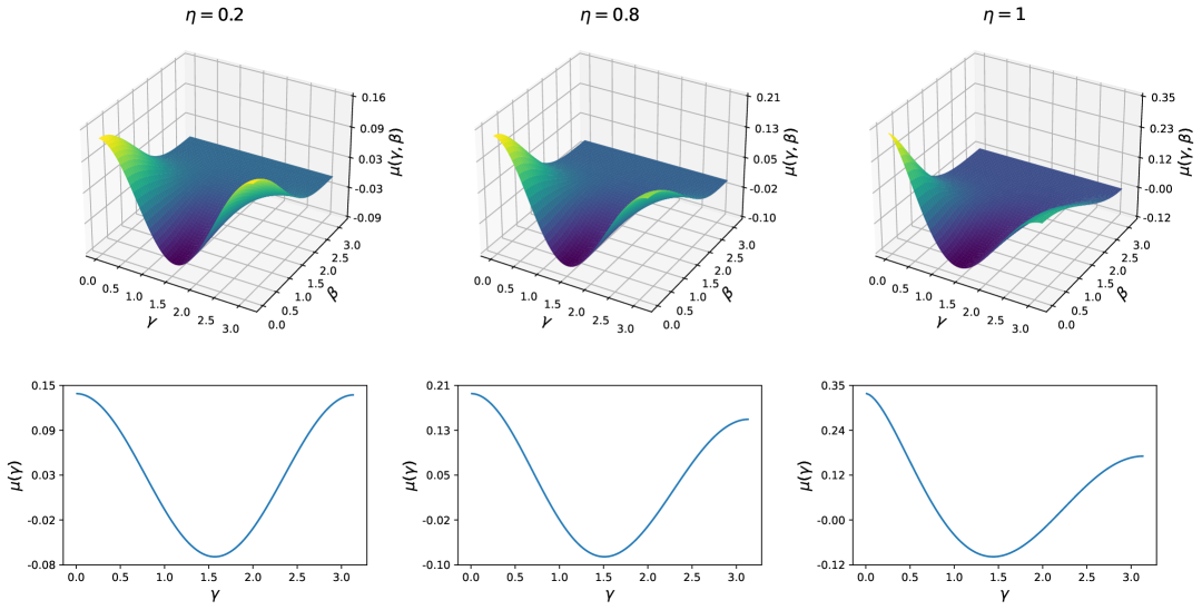
Figure 1: Upper panel: The two-point function $\mu(\gamma,\beta)$ calculated using Eq. (III), representing the mean correlation between two pulsars separated by an angle $\gamma$, arising from two interfering sources with angular separation $\beta$. Three representative cases are shown for $\eta=0.2$, $0.8$, and $1$. Lower panel:The corresponding correlation $\mu(\gamma)$ obtained from Eq. (26) by setting $\beta=0$ in $\mu(\gamma,\beta)$. This recovers the standard angular correlation when only auto-interference is considered. The same three cases, $\eta=0.2$, $0.8$, and $1$, are shown.

While the auto-interference term leads to a well-defined and predictable structure, the contribution from mutual interference between GW sources is inherently unpredictable, as it depends on source-specific information such as individual phases and sky locations—quantities that are generally inaccessible. As a result, the full correlation curve given in Eq. (20) also becomes unpredictable. To explore its statistical properties, we therefore turn to numerical simulations.

We generate 1,000 realizations of the correlation for the representative cases with $\eta=0.2$, $0.8$, and $1$. In each realization, 1,000 GW sources are uniformly distributed over the sky with random directions $\Omega_{j}$ and random phases $\phi_{j}$. The amplitudes $A_{j}$ are drawn from a uniform distribution over the interval [0.01, 1]. The resulting normalized correlations are shown in Fig. 2: the pink curves represent individual realizations, the blue dotted line shows the mean correlation across all realizations, and the green dashed lines indicate the region within one standard deviation of the mean.

To investigate the detailed structure of the full correlation, we expand each curve in terms of Legendre polynomials as

$$\Gamma(\gamma)=\sum_{l}q_{l}P_{l}(\cos\gamma),$$ (27)

where $P_{l}(\cos\gamma)$ denotes the Legendre polynomial of order $l$ evaluated at angle $\gamma$, and $q_{l}$ are the corresponding Legendre coefficients, which vary from realization to realization. Violin plots illustrating the distributions of $q_{l}$ up to the fifth order are presented in Fig. 3. We find that, overall, the monopole ($l=0$) and dipole ($l=1$) components contribute negligibly, while significant contributions emerge at $l\geq 2$ but diminish with increasing $l$. Moreover, the dominance of the quadrupole ($l=2$) component becomes increasingly pronounced as $\eta$ decreases, consistent with the more symmetric trend observed in Fig. 2. These features reflect both the intrinsic quadrupolar nature and the effects of the modified dispersion relation of GW radiation.

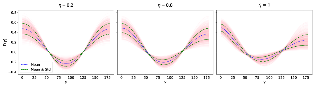
Figure 2: Normalized correlation curves $\Gamma(\gamma)$ from 1,000 realizations for $\eta=0.2$, $0.8$, and $1$. Pink curves represent individual realizations, the blue dotted line indicates the mean correlation, and the green dashed lines denote the one-standard-deviation range around the mean.

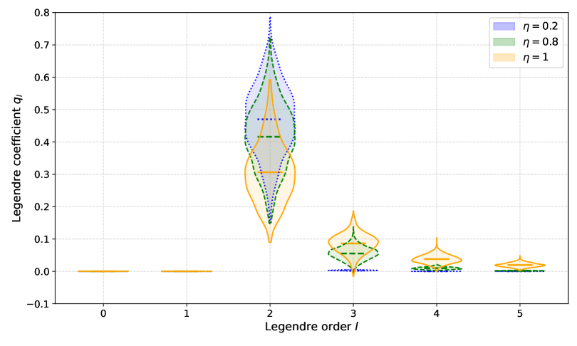
Figure 3: Violin plots of the coefficients $q_{l}$ from the Legendre polynomial decomposition Eq. (27) of the full normalized correlation $\Gamma(\gamma)$, shown up to the fifth order and based on 1,000 simulations. The purple violins with dotted outlines, green violins with dashed outlines, and yellow violins with solid outlines correspond to the cases of $\eta=0.2$, $0.8$, and $1$, respectively. Horizontal lines indicate the means of the distributions.

IV Summary and Discussion

In the nanohertz band, numerous GW sources emitting at similar frequencies interfere with one another. As a result, the spatial correlation pattern induced by a realistic SGWB in PTAs is shaped by such interference, deviating from the conventional correlation derived under the assumption of an isotropic Gaussian ensemble of sources.

In this work, we investigate how GW interference affects the spatial correlation function in the context of massive gravity. Through simulations, we demonstrate that the resulting angular correlations—determined by specific interference configurations—are well characterized by a Legendre polynomial expansion. These correlations predominantly receive contributions from modes with $l\geq 2$, with the coefficients generally decreasing as $l$ increases. Moreover, as the graviton mass increases (for a fixed frequency), the quadrupole component ($l=2$) becomes increasingly dominant. These trends reflect both the quadrupolar nature intrinsic to GW radiation and the modified dispersion relation arising in massive gravity.

While it has been anticipated that spatial correlation measurements in PTAs could help distinguish massive gravity from GR, GW interference poses a significant complication. Since we can observe only a single Universe—with a fixed (albeit unknown) configuration of GW source positions and phases—we cannot rely on statistical averaging over multiple realizations to discriminate between theories. On the other hand, many possible interference configurations can produce angular correlation patterns that are consistent with either theory (see Fig. 2), making it difficult to draw a clear distinction from a single realization.

We now consider this issue in greater detail. In PTA data analysis, an SGWB is characterized by the cross-power spectral density $S_{AB}(f)=P(f)\Gamma(\gamma_{AB})$ at discrete Fourier frequencies $f_{i}=i/T$ ($i=1,2,\cdots$), where $P(f)$ is the power spectral density of the GWB. In principle, both $P(f)$ and $\Gamma(\gamma_{AB})$ can provide insights into physics consistent or beyond GR.

From Eq. (2), we note that a nonzero graviton mass implies a minimum allowed frequency for GWs, given by

$$f_{\text{min}}=\frac{m_{g}}{2\pi}.$$ (28)

For a PTA operating over a timespan $T$, the absence of power in $P(f)$ below a certain frequency may indicate the presence of a graviton mass. Conversely, if $P(f)$ remains nonzero at the lowest accessible frequency $1/T$, this sets a fundamental upper bound on the graviton mass,

$$m_{g}\leq m_{b}=\frac{2\pi}{T}.$$ (29)

One might consider tightening this constraint using angular correlation information—for example, imposing $m_{g}<1/2\,m_{b}$. This case, $m_{g}=1/2\,m_{b}$, corresponds to values of $\eta=0.866$, $0.968$, $0.986$, $0.992$, and $0.995$ in the first five frequency bins, respectively. However, since $\eta$ increases with frequency and asymptotically approaches unity in the massless limit, averaging angular correlations across frequency bins—as is valid in GR Allen and Romano (2025)—is not justified. Instead, constraints must rely on individual frequency bins, particularly the lowest one, which exhibits the strongest deviation from $\eta=1$.

Nevertheless, even in the cases of $\eta=0.8$ and $\eta=1$, our simulations, as shown in Fig. 3, clearly indicate that their Legendre coefficients largely overlap with each other for the dominant $l=2$ and $l=3$ modes. This suggests that the ability to distinguish between these two scenarios is very limited, even under ideal, noise-free conditions. In realistic observational settings, noise further degrades the precision with which these coefficients can be measured—as demonstrated by the NANOGrav 15-year results shown in Fig. 7—making it even more challenging to resolve such subtle differences.

Therefore, once realistic GW interference from different sources is accounted for, the angular correlation function is unlikely to yield a substantial improvement in the graviton mass constraint beyond the spectral bound set by the lowest observable frequency.

It is important to note, however, that such interference effects are primarily relevant for GW backgrounds of astrophysical origin. In contrast, for a cosmological GW background—such as those produced by first-order phase transitions or cosmic strings—the ergodic hypothesis applies Caprini and Figueroa (2018). The reason is that the present-day GWB results from the superposition of many independent signals emitted by uncorrelated regions in the early Universe. As a result, we effectively access multiple realizations and can observe a predictable, ensemble-averaged correlation pattern, which theoretically retains distinctive features capable of discerning a massive graviton.