FMaMIL: Frequency-Driven Mamba Multi-Instance Learning for Weakly Supervised Lesion Segmentation in Medical Images

Abstract

Accurate lesion segmentation in histopathology images is essential for diagnostic interpretation and quantitative analysis, yet it remains challenging due to the limited availability of costly pixel-level annotations. To address this, we propose FMaMIL, a novel two-stage framework for weakly supervised lesion segmentation based solely on image-level labels. In the first stage, a lightweight Mamba-based encoder is introduced to capture long-range dependencies across image patches under the MIL paradigm. To enhance spatial sensitivity and structural awareness, we design a learnable frequency-domain encoding module that supplements spatial-domain features with spectrum-based information. CAMs generated in this stage are used to guide segmentation training. In the second stage, we refine the initial pseudo labels via a CAM-guided soft-label supervision and a self-correction mechanism, enabling robust training even under label noise. Extensive experiments on both public and private histopathology datasets demonstrate that FMaMIL outperforms state-of-the-art weakly supervised methods without relying on pixel-level annotations, validating its effectiveness and potential for digital pathology applications. The code can be accessed at https://github.com/chenghangbei0702/FmaMIL.

We propose FMaMIL, the first Mamba-based MIL framework enhanced with learnable frequency-domain encoding for weakly supervised lesion segmentation using only image-level labels.

A bidirectional spatial scanning strategy is introduced to model contextual structures in pathology images more effectively.

A CAM-guided pseudo-label refinement strategy with soft supervision and self-correction enhances segmentation under label noise.

Our method achieves state-of-the-art segmentation performance on both public and private histopathology datasets without relying on pixel-level annotations.

1 Introduction

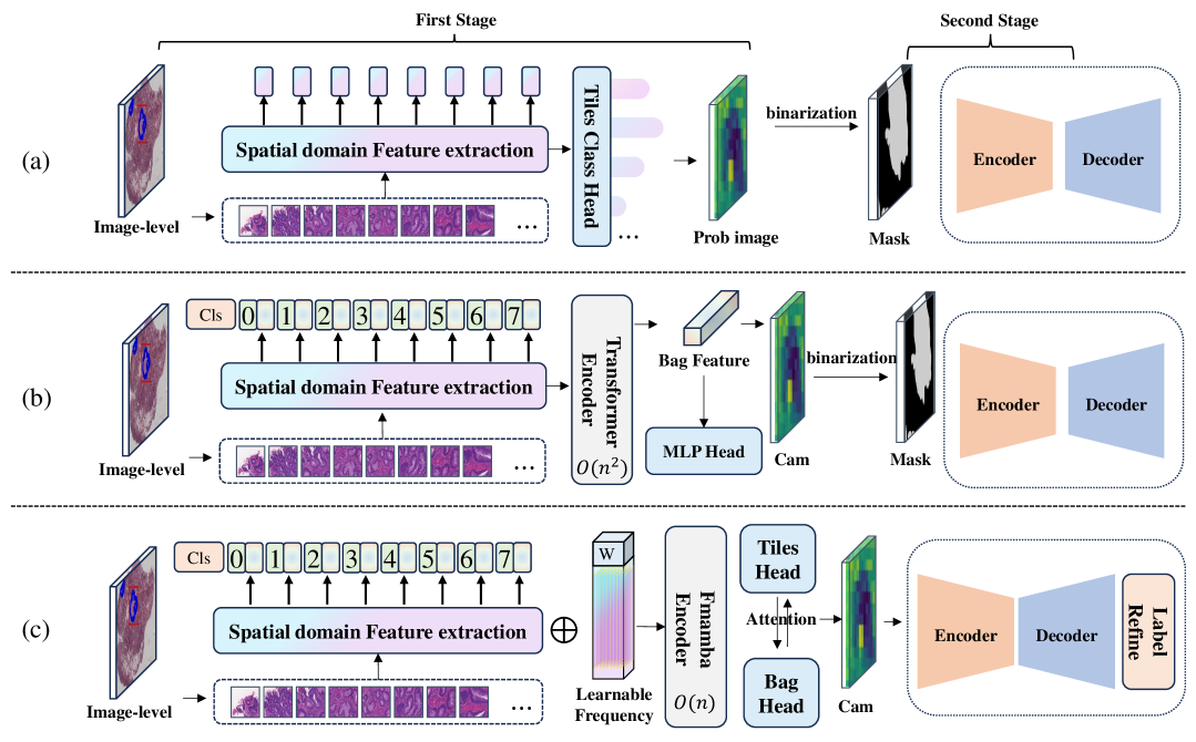
Figure 1: Comparison of three two-stage WSS frameworks for pathology images. (a) Tile classification-based method for generating pseudo masks; (b) Transformer-based MIL with attention map generation; (c) Our proposed method, which incorporates learnable frequency features and a lightweight Mamba encoder to achieve efficient and accurate mask generation with label refinement..

In the field of digital medicine, ultra-high-resolution whole-slide images (WSIs) have become a mainstream imaging modality for modern disease diagnosis due to their comprehensive and rich diagnostic information[54, 65, 22, 35, 12]. However, accurately identifying abnormal tissue regions in such high-resolution and structurally complex pathological images poses a significant challenge. These abnormal regions often exhibit subtle and diffuse structural features, as illustrated in Fig. 2, creating substantial difficulties for automated analysis. Traditional supervised segmentation methods rely heavily on high-quality pixel-level annotations provided by experienced medical experts, which are both time-consuming and expensive[53]. Moreover, the subjectivity involved in annotation can lead to substantial variability in labeling results for the same lesion, further undermining the generalization capability of models[34]. Consequently, patient-level labels, as the most readily available form of coarse annotation in clinical practice, have gained attention for weakly supervised lesion segmentation, offering an effective strategy to alleviate the reliance on high-quality data annotations[56, 2].

Segmentation methods based on patient-level labels provide only pathological category information without specifying lesion locations, making this approach one of the most challenging problems in pixel-level segmentation tasks[36, 38]. Due to GPU memory constraints, traditional weakly supervised segmentation(WSS) methods cannot directly process WSIs comprising billions of pixels[55], and multiple instance learning (MIL) has emerged as the predominant solution[46]. MIL operates under a bag-based learning paradigm, where each bag comprises multiple instances, and labels are provided only at the bag level while individual instance labels remain unknown[10]. In pathological image analysis, a WSI is considered positive if it contains any lesion areas[36, 47]. By leveraging this strategy, feature extraction is performed on small instances within the MIL framework rather than on the gigapixel WSI, alleviating GPU memory limitations[46, 49].

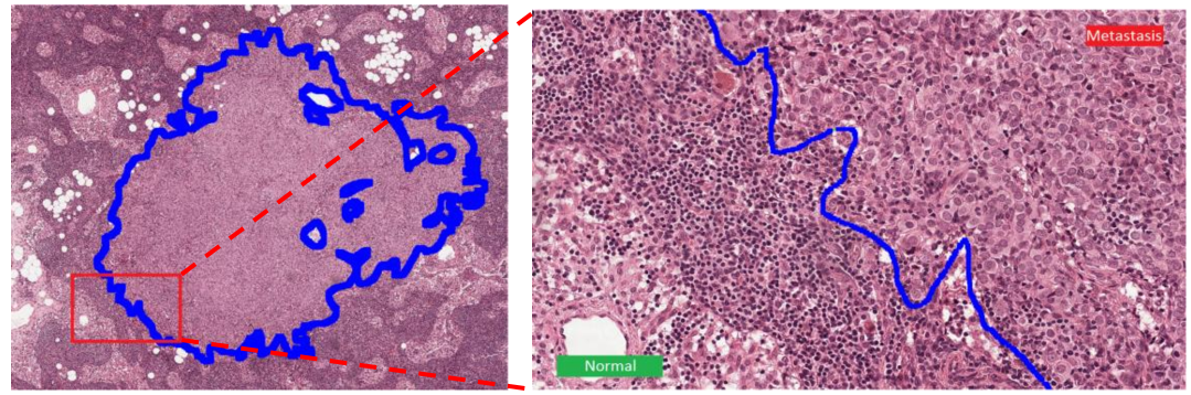
Figure 2: illustrates the common diffuse characteristics of lesions.

Conventional MIL tasks typically encode instances within a bag into low-dimensional features using pre-trained models and aggregate these features into bag-level representations [24, 8]. In this process, instances within the bag are often assumed to be independent and identically distributed (i.i.d.), resulting in loss functions that backpropagate only to a subset of prominent positive instances, potentially leading to false segmentation issues [24, 58], as exemplified in tile classification-based frameworks(Fig. 1(a)). In contrast, clinical pathologists consider not only contextual information around regions but also the interrelations between different regions during diagnosis[36, 46]. Consequently, recent studies have reformulated WSI analysis as a long-sequence modeling problem[67, 49], employing models like Transformers (Fig. 1(b)) to capture discriminative features by exploring inter-instance correlations and global contextual information at the bag level. Despite improvements in performance, such methods face challenges of high computational cost and overfitting, limiting further advancements[70]. Recently, the selective state-space model (Mamba) was introduced as a novel approach to address the computational complexity bottleneck of Transformers[44, 23, 51]. Mamba achieves linear computational complexity without compromising the global receptive field, significantly enhancing efficiency. Studies have demonstrated Mamba’s superior ability to capture long-range dependencies, surpassing traditional models. Unlike typical visual tasks, WSIs exhibit weak spatial correlations and sparse distributions of positive patches, making Mamba’s robust sequential modeling capabilities particularly advantageous for WSI analysis. Interestingly, although some methods have combined Mamba with MIL, these efforts have primarily focused on image classification, with limited attention to the more challenging segmentation tasks[67, 15]. Furthermore, existing research predominantly extracts features in the spatial domain, neglecting the potential value of frequency-domain information[20]. Frequency-domain features uniquely excel in capturing texture and edge details in pathological images, especially in noisy or complex backgrounds[5, 63]. Therefore, integrating multi-level features from both spatial and frequency domains holds promise for further performance improvements.

Based on this background, we propose FMaMIL, a novel Mamba MIL framework that integrates frequency-domain and spatial-domain information for weakly supervised lesion segmentation in digital pathology, as illustrated in Fig. 1(c). The proposed framework leverages Mamba’s linear computational advantages in long-range feature extraction to thoroughly explore inter-instance correlations, while frequency-domain information enhances feature representation to better understand the complex characteristics of lesions. FMaMIL demonstrates excellent scalability, effectively mining instance-level features while ensuring bag-level classification accuracy. We evaluate the proposed method on two datasets, including one private and one public datasets. Experimental results show that our model significantly outperforms state-of-the-art methods, achieving superior performance and strong generalization in lesion segmentation tasks.

The major contributions of this paper are summarized as follows:

• To the best of our knowledge, we are the first to propose FMaMIL—a novel weakly supervised lesion segmentation framework that integrates Mamba-based long-range modeling and learnable frequency-domain encoding under the MIL paradigm, using only image-level labels.

• A learnable frequency-domain encoding module and a bidirectional spatial scanning mechanism are introduced to enhance the model’s ability to capture texture details and contextual structure.

• We design a CAM-guided pseudo-label refinement strategy with soft supervision and self-correction, enabling coarse-to-fine training and achieving state-of-the-art performance on two histopathology datasets.

The remainder of this paper is organized as follows: Section 2 reviews the related work, highlighting the limitations and challenges in the field. Section 3 focuses on the proposed method, detailing its design and key technical aspects. Section 4 presents experimental results on three datasets and analyzes ablation studies. Section 5 discusses the strengths and limitations of the model Finally, Section 6 concludes the paper and outlines future research directions.

2 Related works

2.1 Weakly supervised medical image seg.

Weakly supervised medical image segmentation primarily relies on points [3], bounding boxes [9], and image-level annotations [66, 52]. Image-level annotations, being the easiest form of labels to obtain clinically in medicine, have become the mainstream approach. Existing WSSS methods based on image-level labels can mainly be divided into single-stage methods [1] and two-stage methods [60]. Single-stage methods directly use image-level labels as supervision to train end-to-end segmentation networks, while two-stage methods typically involve two separate training steps: converting image-level labels into offline class activation maps (CAM) [73], which highlight the regions in the image that are most influential for classification decisions through heatmap generation, thereby transforming image-level labels into pixel-level pseudo-labels. These pseudo-labels are then used to train segmentation models to improve segmentation accuracy. However, pseudo-labels often contain noise [61], which directly affects the output quality of segmentation models. To improve the quality of attention maps, several improved CAM methods have been proposed, including adversarial erasing [59], online attention accumulation [26], and region growing. Although these methods have made improvements, they usually take the entire image as the only input, are prone to background noise interference, and mainly extract global image information. Especially in digital pathology images, the lesion areas are similar to the background [4], and digital pathology images have the characteristics of high resolution and complex structure [62], making traditional deep learning methods difficult to effectively deal with. MIL [43] has emerged as an effective solution, which processes bags containing multiple instances and relies only on bag-level labels, effectively solving the problem of pathology image segmentation [24, 30].

2.2 Application of MIL in Pathological Seg.

MIL utilizes image-level annotations as labels and segments pathological images into multiple patches. These patches do not have independent labels but are associated only with image-level annotations. MIL effectively addresses the challenges posed by the high resolution and sparse annotations in WSIs[4], achieving a balance between efficiency and effectiveness [32]. Traditional MIL frameworks can be divided into instance-level algorithms and embedding-level algorithms. Kanavati et al. [28] trained a CNN based on the EfficientNet-B3 architecture using transfer learning and MIL, with a focus on the most representative instances. Ilse et al. [24] extracted instance features using a CNN and aggregated these features via an attention mechanism to identify key instances. However, traditional MIL methods typically rely on the assumption of iid instances, extracting features from individual instances only. In clinical practice, pathologists not only rely on features within regions but also pay attention to the relationships between different regions. The aforementioned methods all neglect the correlations between instances [67].

To address this issue, several solutions have been explored. Zhuchen Shao et al. proposed a novel model, TransMIL, based on a correlated multi-instance learning framework [49]. This model integrates morphological and spatial information through manually designed transformation functions and models the correlations between instances using the self-attention mechanism of Transformers, thereby capturing comprehensive image information. Z. Chen et al. introduced the SA-MIL model [32], which incorporates self-attention and deep supervision mechanisms into the standard MIL framework to capture contextual information from the entire image, overcoming the limitations of independent instances. Fang et al. proposed the SAM-MIL framework[14], which addresses the issue of ignoring spatial relationships between instances in traditional MIL methods by introducing spatial information and context-aware mechanisms. However, these methods consume substantial memory resources and have high computational complexity when dealing with higher-dimensional data and complex pathological image structures. Enhancing the model’s ability to process long sequences and improving memory efficiency in WSS of pathological images have become critical issues that urgently need to be resolved in the scientific community.

2.3 Applications of Mamba in Medical Imaging

To achieve high-precision segmentation, multi-instance segmentation is often combined with computationally intensive models such as Transformers, which pose significant challenges when processing long-sequence inputs, such as medical images[50, 29, 19]. To improve efficiency, State-Space Models (SSM)[31, 18] have emerged. This model maps sequential data to a lower-dimensional state space and utilizes matrix or convolution operations for modeling, thereby achieving linear complexity. The Mamba model[57, 17], based on SSM, incorporates global receptive fields and selective scanning operators, expanding the range of information capture while reducing computational load and capturing critical features. These advantages have led to renewed interest in SSM within the academic community.

As Mamba technology has evolved, it has increasingly integrated with other techniques. In visual tasks, Vision Mamba [75] enhances the efficiency of visual feature extraction by processing long-sequence medical images using selective scanning mechanisms, position-awareness, and bidirectional SSM. VMamba[39] effectively collects contextual information from different perspectives through four scanning paths. In MIL tasks, the MamMIL model[15] applies SSM for the first time within the WSI MIL framework, achieving WSI classification with linear complexity. The MambaMIL model [67]enhances long-sequence modeling through a sequence reordering module to improve WSI analysis performance. Mamba2MIL[71] further refines the MambaMIL model by introducing multi-scale analysis to capture additional details. These studies demonstrate that the Mamba framework significantly enhances medical image segmentation accuracy while improving computational efficiency, signaling its broad application potential in medical image analysis. However, it is worth noting that most current research focuses on spatial domain information, whereas frequency domain information is equally critical in medical image analysis[37, 16].

2.4 Frequency-Domain Information in WSIs Seg.

In recent years, frequency-domain information has gained increasing recognition for its ability to effectively integrate global and local feature modeling, highlighting its importance in pathological image segmentation [11, 48, 6, 72, 20, 74]. For instance, FourierMIL [72] leverages Discrete Fourier Transform (DFT) and All-Pass Frequency Filtering to effectively capture both global and local dependencies in the frequency domain, significantly improving classification and segmentation performance for pathological images, particularly in high-resolution WSI analysis. Similarly, T-Mamba [20] integrates frequency-domain features with spatial-domain features by employing a frequency enhancement module and an adaptive gating unit, achieving substantial improvements in the segmentation accuracy of dental CBCT images. This approach demonstrates strong advantages, especially when handling noisy and low-contrast pathological images. Furthermore, Zhou et al. proposed the Spatial-Frequency Dual-Domain Attention Network [74], which utilizes 2D Discrete Fourier Transform (2D-DFT) to separate low- and high-frequency components of images, combined with adaptive filtering to enhance global feature learning, thereby improving the segmentation performance of pathological images.

Despite the significant potential of frequency-domain information in pathological image segmentation, its application still faces several challenges. For example, most filter thresholds require manual tuning, which limits adaptability, and integrating frequency-domain information with spatial-domain features remains difficult. Future research should focus on optimizing adaptive filtering strategies and developing efficient fusion mechanisms to further promote the application of frequency-domain techniques in pathological image segmentation.

3 Proposed method

In this section, we first introduce the relevant prior knowledge, followed by a detailed explanation of the proposed framework. Specifically, we analyze the key components of the framework, including the design of the FMamba block, the learnable frequency-domain encoding, the multi-instance classification head and the Cam-seg Model, along with their technical details.

3.1 Preliminaries

3.1.1 Mamba

Recently, SSM-based methods have demonstrated significant potential in the field of sequential data processing, with particular attention to structured state-space sequence models (S4) and selective state-space models (Mamba). These models rely on classical continuous system theory and leverage efficient algorithms and architectures to process one-dimensional functions or sequences $x(t)\in\mathbb{R}$ through hidden states $h(t)\in\mathbb{R}^{N}$ and map them to outputs $y(t)\in\mathbb{R}$. This mapping process is achieved through carefully designed evolution parameters $\mathbf{A}\in\mathbb{R}^{N\times N}$ and projection parameters $\mathbf{B}\in\mathbb{R}^{N\times 1}$ and $\mathbf{C}\in\mathbb{R}^{1\times N}$

In the continuous-time domain, this process can be represented as a linear ordinary differential equation:

$$h^{\prime}(t) =\mathbf{A}h(t)+\mathbf{B}x(t),$$ (1)

$$y(t) =\mathbf{C}h(t).$$

where $\mathbf{A}$ serves as the evolution matrix for hidden states, $\mathbf{B}$ describes the influence of input signal $x(t)$ on hidden states, and $\mathbf{C}$ is responsible for extracting the output from hidden states, $h^{\prime}(t)$ denotes the rate of change of the hidden state over time.

To apply this continuous system to discrete-time scenarios, S4 and Mamba models introduce a time-scale parameter $\Delta$ and use discretization methods such as Zero-Order Hold (ZOH) to convert continuous parameters $\mathbf{A}$ and $\mathbf{B}$ into discrete parameters $\overline{\mathbf{A}}$ and $\overline{\mathbf{B}}$. This process typically follows the following formulas:

$$\begin{split}\overline{\mathbf{A}}&=\exp(\Delta\mathbf{A}),\\ \overline{\mathbf{B}}&=(\Delta\mathbf{A})^{-1}(\exp(\Delta\mathbf{A})-\mathbf{I})\cdot\Delta\mathbf{B}.\end{split}$$ (2)

$\exp(\cdot)$ denotes the matrix exponential, serving as a bridge between continuous and discrete-time systems.

In the discrete-time domain, the state equation and output equation of the state-space model can be expressed as:

$$\begin{split}h_{t}&=\overline{\mathbf{A}}h_{t-1}+\overline{\mathbf{B}}x_{t},\\ y_{t}&=\mathbf{C}h_{t}.\end{split}$$ (3)

At the end of the process, by computing the convolution kernel $\overline{\mathbf{K}}\in\mathbb{R}^{M}$ of the SSM, the model can efficiently extract features from the input sequence x and generate the output sequence y. This process can be represented as:

$$\begin{split}\overline{\mathbf{K}}&=(\mathbf{C}\overline{\mathbf{B}},\mathbf{C}\overline{\mathbf{A}}\overline{\mathbf{B}},\ldots,\mathbf{C}{\overline{\mathbf{A}}}^{M-1}\overline{\mathbf{B}}),\\ \text{y}&=\text{x}*\overline{\mathbf{K}}.\end{split}$$ (4)

Here, $M$ denotes the length of the input sequence $x$.

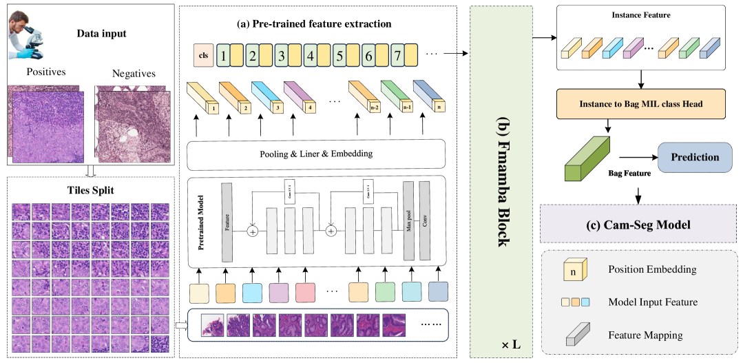
Figure 3: The overall framework of our proposed FMaMIL primarily consists of three stages.

3.1.2 Multiple Instance Learning

In the process of MIL, the data is organized into bags rather than instances, The instances do not have labels. let $W=\{(x_{1},y_{1}),...,(x_{n},y_{n})\}$ represent a WSI bag $W$, where $n$ represents the total number of patches contained in $W$. Each individual yield instance-level features $x_{i}\in\{x_{1},x_{2},\ldots,x_{n}\}$ has a corresponding latent label $y_{i}\in\{y_{1},y_{2},\ldots,y_{N}\}$ (where $y_{i}$ = 1 denotes positive, and $y_{i}$ = 0 denotes negative). The labels $y$ for bag $W$ are known to the model and are represented as follows:

$$y(W)=\begin{cases}0,&\text{if}\sum_{i=1}^{K}y_{i}=0,\\ 1,&\text{otherwise}.\end{cases}$$ (5)

When at least one instance in the bag $W$ is classified as positive, the WSI is classified as positive; otherwise, it is classified as negative. MIL decomposes high-resolution images into multiple small image patches, which has been shown to extract more microstructural information about the lesions.

3.2 The overall framework

We propose an innovative WSS strategy that integrates MIL with the Mamba, cleverly combining frequency-domain and spatial-domain feature information. We refer to this approach as FMaMIL. As shown in Fig. 3, the proposed method framework is carefully designed with three core stages: Pre-trained Feature Extraction, deep exploration of instance correlations, and a pseudo-label training strategy based on the CAM.

In the deep exploration of instance correlations stage, we further introduce a learnable frequency-domain encoding technique and a bidirectional scanning mechanism for spatial-domain features. In the following subsections, we will detail the specific implementation of each stage.

3.3 pre-trained feature extraction

Our framework is designed to process pathological slice data containing both positive and negative samples, including positive sample set $D^{+}=\{\mathbf{S}_{1}^{+},\mathbf{S}_{2}^{+},\ldots,\mathbf{S}_{a}^{+}\}$ and the negative sample set $D^{-}=\{\mathbf{S}_{1}^{-},\mathbf{S}_{2}^{-},\ldots,\mathbf{S}_{b}^{-}\}$. Each pathological slice $\mathbf{S}_{a}^{+}$ or $\mathbf{S}_{b}^{-}\in\mathbb{R}^{\mathtt{H\times W\times C}}$ is further divided into $N\times M$ non-overlapping image patches. $N$ for the number of rows, $M$ for the number of columns. $(H,W)$ represents the dimensions of the input image, and $C$ is the number of channels. Each patch $\mathbf{p}_{(n,m)}\in\{\mathbf{p}_{(1,1)},\mathbf{p}_{(1,2)},\ldots,\mathbf{p}_{(N,M)}\}\in\mathbb{R}^{\mathtt{q\times q\times C}}$ carries detailed information and tissue structure from a local region of the pathological slice. $q$ represents the size of the side length of a patch.

Next, we use a pre-trained Convolutional Neural Network, such as ResNet, VGG, or EfficientNet, to extract features from each patch $\mathbf{p}_{(n,m)}$. This process captures diverse features ranging from low-level details (e.g., edges and textures) to high-level semantic information (e.g., tissue types and lesion characteristics), encoding each patch into a fixed-dimensional vector $\mathbf{f}_{(n,m)}\in\mathbb{R}^{d}$. The feature extraction process can be formulated as:

$$\mathbf{f}_{(n,m)}=F_{\text{CNN}}(\mathbf{p}_{(n,m)}),n=1,2,\dots,N,m=1,2,\dots,M,$$ (6)

where $F_{\text{CNN}}$ represents the pre-trained CNN model, and $d$ is the dimension of the feature vector.

After extracting features for all patches, These features are arranged into a sequential order by scanning the spatial positions of the patches row by row in the original image, forming a sequence:

$$\mathbf{F}_{row}=[\mathbf{f}_{(1,1)},\mathbf{f}_{(1,2)},\dots,\mathbf{f}_{(n,m)}]\in\mathbb{R}^{N\times M\times d}.$$ (7)

Next, positional encoding is added to each feature vector $\mathbf{f}_{(n,m)}$ to retain spatial positional information of the image. Additionally, a learnable classification token (cls token), initialized as a zero vector $\mathbf{f}_{\text{cls}}\in\mathbb{R}^{d}$, is prepended to the sequence. The final input sequence after adding the CLS token can be expressed as:

$$\mathbf{F}^{\prime}_{row} =[\mathbf{f}_{\text{cls}},\mathbf{f}_{(1,1)}+\mathbf{e}_{1},\mathbf{f}_{(1,2)}+\mathbf{e}_{2},\dots,\mathbf{f}_{(n,m)}+\mathbf{e}_{N\times M}]$$ (8)

$$\in\mathbb{R}^{(N\times M+1)\times d}$$

where $\mathbf{e}_{i}\in\mathbb{R}^{d}$ represents the positional encoding for the $i$-th patch.

3.4 deep exploration of instance correlations

To fully explore the correlations between samples and reconstruct the structural information of images in two-dim space based on realistic visual scanning patterns, this section will first introduce the sentence reordering technique, followed by the design of a learnable frequency-domain encoding. Finally, the overall encoder architecture based on Mamba and dual-domain information will be presented.

3.4.1 Sentence reordering

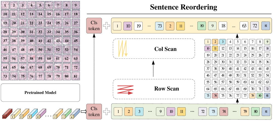
Figure 4: Sentence Reordering Structure.

After the pre-training phase, we obtain the feature sequence $\mathbf{F}^{\prime}_{row}$ for each pathology slide, which is generated through row-wise scanning in two-dimensional space. However, during inference, the model may overlook information from the vertical spatial dimension. To address this, we designed a sentence reordering technique to transform the row-wise feature sequence $\mathbf{F}^{\prime}_{row}$ into a column-wise feature sequence $\mathbf{F}^{\prime}_{col}$. The detailed process is illustrated in Fig. 4.

Specifically, the sentence reordering technique reorganizes the patch feature sequence based on their column positions in the original pathology slide, rather than their row positions. In the newly generated column-wise sequence, each patch retains its original feature vector, but their arrangement is adjusted according to the column indices. The reordered feature sequence can be expressed as:

$$\mathbf{F}^{\prime}_{col} =[\mathbf{f}_{\text{cls}},\mathbf{f}_{(1,1)}+\mathbf{e}_{1},\mathbf{f}_{(2,1)}+\mathbf{e}_{2},\dots,\mathbf{f}_{(m,n)}+\mathbf{e}_{M\times N}]$$ (9)

$$\in\mathbb{R}^{(N\times M+1)\times d}$$

where $\mathbf{f}_{(m,n)}$ represents the feature vector of the patch located at the $m$-th row and $n$-th column.

In addition, we incorporate positional encodings and an extra learnable classification token (CLS token) into the new column-wise sequence $\mathbf{F}^{\prime}_{col}$. This allows the model to differentiate and effectively process the two scanning modes (row-wise and column-wise), thereby capturing the spatial structural information of the pathology slides more comprehensively.

3.4.2 learnable frequency-domain encoding

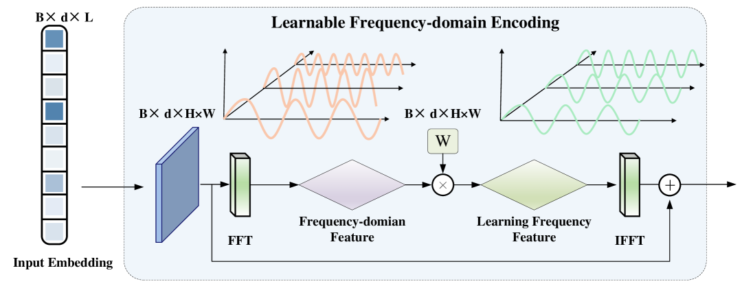
Figure 5: Learnable Frequency Domain Encoding Structure.

Features extracted in the spatial domain typically capture local spatial details and dependencies. However, the frequency domain offers a different perspective, focusing on the frequency components and global patterns of the data. This is crucial for modeling long-range dependencies. High-resolution digital pathology images often contain substantial local details, such as cellular structures, interstitial spaces, and blood vessels. Unlike traditional classification methods, MIL relies more heavily on understanding local texture details (corresponding to high-frequency signals in the frequency domain) and global structural features (corresponding to low-frequency signals in the frequency domain). The fusion of these multi-scale features is particularly important for effective pseudo-segmentation tasks.

Frequency domain encoding helps models capture hierarchical spatial information and organizational structures more effectively. Based on this idea, we propose the use of Fast Fourier Transform (FFT) to build learnable frequency domain encoding with logarithmic-linear computational complexity, achieving more comprehensive feature extraction. This approach can be viewed as a trainable frequency filter that automatically learns the relevant frequency components for classification while suppressing unrelated signals. This operation also helps reduce the computational burden on the network.

Algorithm 1 Learnable Frequency Domain Encoding

Require: token sequence $\mathbf{x}_{f}:{\color[rgb]{0,0.46875,0}\mathtt{(B,M,E)}}$
Ensure: token sequence $\mathbf{y}_{f}:{\color[rgb]{0,0.46875,0}\mathtt{(B,M,E)}}$

1:/* FFT branch for frequency domain processing */

2:$\mathbf{x^{\prime}}_{f}:{\color[rgb]{0,0.46875,0}\mathtt{(B,M,E)}}\leftarrow\mathbf{FFT}(\mathbf{x}_{f})$

3:$\mathbf{x^{\prime}}_{f}:{\color[rgb]{0,0.46875,0}\mathtt{(B,M,E)}}\leftarrow\mathbf{x^{\prime}}_{f}\bm{\odot}\mathbf{W}_{f}$

4:/* dd learnable parameters */

5:$\mathbf{x^{\prime}}_{f}:{\color[rgb]{0,0.46875,0}\mathtt{(B,M,E)}}\leftarrow\mathbf{LearnableParameters}(\mathbf{x^{\prime}}_{f})$

6:/* IFFT branch and follow-up actions */

7:$\mathbf{x^{\prime}}_{f}:{\color[rgb]{0,0.46875,0}\mathtt{(B,M,E)}}\leftarrow\mathbf{IFFT}(\mathbf{x^{\prime}}_{f})$

8:/* add skip connection */

9:$\mathbf{y}_{f}:{\color[rgb]{0,0.46875,0}\mathtt{(B,M,E)}}\leftarrow\mathbf{x^{\prime}}_{f}+\mathbf{x}_{f}$

10:$\mathbf{Return}:\mathbf{y}_{f}$

Architecture: The learnable frequency domain encoding approach is based on a spectral network composed of an FFT layer, a learnable encoding module, and an inverse FFT (IFFT) layer. The detailed process is illustrated in Fig. 5 and Algorithm. 1.

First, the input feature tensor $x\in\mathbb{R}^{B\times d\times L}$, where $B$ is the batch size,and $L$ is the sequence length. We apply FFT along the sequence dimension $L$, converting the feature from the spatial domain to the frequency domain, yielding the complex frequency domain representation $x_{\text{fft}}$, which consists of real part $x_{\text{fft\_real}}$ and imaginary part $x_{\text{fft\_imag}}$. This process can be represented as:

$$\begin{split}x_{\text{fft}}&=\text{FFT}(x),\\ X[k]&=\sum_{n=0}^{L-1}x[n]\cdot e^{-j\frac{2\pi}{L}kn},\quad k=0,1,\ldots,L-1,\\ x_{\text{fft}}&=x_{\text{fft\_real}}+j\cdot x_{\text{fft\_imag}}\end{split}$$ (10)

where $x[n]$ is the $n$-th element of the input sequence, $X[k]$ is the $k$-th frequency component in the frequency domain, $j$ is the imaginary unit.

Secondly,unlike traditional filtering methods, we use learnable weight parameters to automatically learn the importance of each frequency component, thus capturing both coarse and fine spatial features. This approach enhances the model’s flexibility and robustness. Specifically, we introduce learnable frequency weights $w\in\mathbb{R}^{D\times L}$ for each channel. The complex weights include both real and imaginary parts. These weights are applied to the frequency domain features using complex arithmetic rules, as follows:

$$x_{\text{fft\_out}}=x_{\text{fft}}\cdot w$$ (11)

Finally, we apply the IFFT to transform the frequency domain features back to the spatial domain $x_{\mathrm{fft\_space}}$. To address the potential loss of local details—particularly the incomplete representation of edges and small objects—caused by the dispersion of information across the entire spectrum during the Fourier Transform (FT), we introduce a skip connection into the operation process. This process can be represented as:

$$\begin{split}x_{\text{fft\_space}}&=x+x_{\text{ifft}}\\ &=x+\frac{1}{N}\sum_{k=0}^{N-1}X_{\text{fft\_out}}[k]e^{j2\pi\frac{kn}{N}}\end{split}$$ (12)

3.4.3 FMamba block

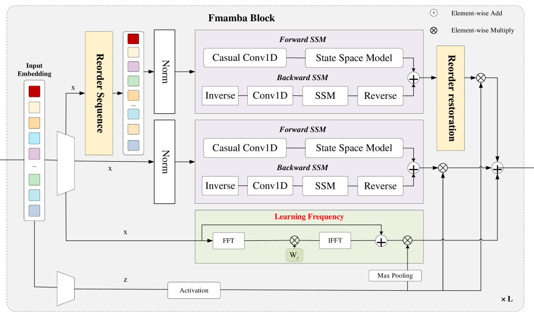
Figure 6: Fmamba Block Structure.

We have previously outlined the fundamental components of the mamba-based encoder within the FaMIL framework. Building upon this foundation, we further present the basic architecture of an enhanced mamba encoding block, which integrates spatial and frequency domain information, as illustrated in Fig. 6 and Algorithm. 2 . In this structure, we extract row-wise scanning sequences ($\mathbf{F}^{\prime}_{row}$), column-wise scanning sequences ($\mathbf{F}^{\prime}_{col}$), and the output of a learnable frequency domain encoding module ($x_{\text{fft\_space}}$) from the input.

In the design of the novel mamba-based module, we draw inspiration from Ref. [69] and introduce a bidirectional sequence modeling strategy to reconstruct finer details in the visual 2D space. Specifically, for the sequences $\mathbf{F}^{\prime}_{row}$ and $\mathbf{F}^{\prime}_{col}$, we first standardize them using normalization layers. Subsequently, the normalized sequences are linearly projected into vectors $x$ and $z$ of dimension $E$. Next, we apply forward and backward SSM operations on $x$. Each directional sequence modeling involves passing through a Casual Convolution Layer followed by an SSM. For the output of sequence $\mathbf{F}^{\prime}_{col}$, we go through the recorder restoration module before converting it into a sequence that corresponds to the progressive scan $\mathbf{F}^{\prime}_{row}$ one by one. Finally, we aggregate the results of the bidirectional sequence modeling using a gating mechanism with $z$, yielding the corresponding outputs $\mathrm{out_{\text{row}}}$ and $\mathrm{out_{\text{col}}}$ for $\mathbf{F}^{\prime}_{row}$ and $\mathbf{F}^{\prime}_{col}$, respectively. This process can be mathematically described as follows:

$$\begin{split}\mathbf{F}^{\prime\prime}&=\mathrm{Norm}(\mathbf{F}^{\prime}),\\ \mathrm{out_{\text{row/col}}}&=\mathrm{SiLu}(z)\cdot(\mathrm{SSM}(\mathrm{Conv}1\mathrm{D}(\mathbf{F}^{\prime\prime}))\\ &\quad+\mathrm{SSM}(\mathrm{Conv}1\mathrm{D}(\mathbf{F}^{\prime\prime}[-1]))[-1])\end{split}$$ (13)

where $\mathbf{F}^{\prime}$ represents the input sequence ( $\mathbf{F}^{\prime}_{row}$ or $\mathbf{F}^{\prime}_{col}$), and $\mathrm{Conv}1\mathrm{D}$ denotes a one-dimensional convolutional layer.

As a supplement, for $x_{\text{fft\_space}}$, the frequency feature is aggregated by the activated $z^{\prime}$ with maxpooling operation. This approach preserves the global information adjusted in the frequency domain while maintaining the local patterns of spatial features. The process can be expressed mathematically as follows:

$$\mathrm{out}_{\text{fft}}=\mathrm{LayerNorm}(|x_{\text{fft\_space}}\cdot\mathrm{Max\_pool}(\mathrm{SiLu}(z))|)$$ (14)

Ultimately, we obtain three key outputs: $\mathrm{out_{\text{row}}}$ , $\mathrm{out_{\text{col}}}$ and $\mathrm{out}_{\text{fft}}$. Unlike the gated weighted fusion operation proposed in Ref. [20], we adopt a more straightforward and concise strategy, directly summing these three outputs to produce a new fused sequence $F_{\mathrm{new}}$. This approach not only preserves spatial information and frequency-domain features more comprehensively but also effectively reduces the computational complexity of the model. The process can be expressed mathematically as:

$$F_{\mathrm{new}}=\mathrm{out_{\text{col}}}+\mathrm{out_{\text{row}}}+\mathrm{out_{\text{fft}}}$$ (15)

Algorithm 2 Fmamba Block Process

Require: token sequence $\mathbf{T}_{l-1}:{\color[rgb]{0,0.46875,0}\mathtt{(B,M,D)}}$
Ensure: token sequence $\mathbf{T}_{l}:{\color[rgb]{0,0.46875,0}\mathtt{(B,M,D)}}$

1:${\color[rgb]{0.5,0.5,0.5}\text{/* normalize the input sequence }\mathbf{T^{\prime}}_{l-1}\text{ */}}$

2:$\mathbf{T^{\prime}}_{l-1}:{\color[rgb]{0,0.46875,0}\mathtt{(B,M,D)}}\leftarrow\mathbf{Norm}(\mathbf{T}_{l-1})$

3:$\mathbf{x}:{\color[rgb]{0,0.46875,0}\mathtt{(B,M,E)}}\leftarrow\mathbf{Linear}^{\mathbf{x}}(\mathbf{T^{\prime}}_{l-1})$

4:$\mathbf{z}:{\color[rgb]{0,0.46875,0}\mathtt{(B,M,E)}}\leftarrow\mathbf{Linear}^{\mathbf{z}}(\mathbf{T^{\prime}}_{l-1})$

5:/* split x into three parts for different directions */

6:$\mathbf{x}_{h},\mathbf{x}_{v},\mathbf{x}_{f}:{\color[rgb]{0,0.46875,0}\mathtt{(B,M,E)}}\leftarrow\mathbf{Split}(\mathbf{x})$

7:/* reorder $x_{v}$ for the vertical direction */

8:$\mathbf{x}_{v}:{\color[rgb]{0,0.46875,0}\mathtt{(B,M,E)}}\leftarrow\mathbf{Reorder}(\mathbf{x}_{v})$

9:/* perform bidirectional propagation for $x_{h}$ and $x_{v}$ separately */

10:for $o\in\{\text{forward},\text{backward}\}$ do

11:  $\mathbf{x^{\prime}}_{o}:{\color[rgb]{0,0.46875,0}\mathtt{(B,M,E)}}\leftarrow\mathbf{SiLU}(\mathbf{Conv1d}_{o}(\mathbf{x}))$

12:  $\mathbf{B}_{o}:{\color[rgb]{0,0.46875,0}\mathtt{(B,M,N)}}\leftarrow\mathbf{Linear}^{\mathbf{B}}_{o}(\mathbf{x^{\prime}}_{o})$

13:  $\mathbf{C}_{o}:{\color[rgb]{0,0.46875,0}\mathtt{(B,M,N)}}\leftarrow\mathbf{Linear}^{\mathbf{C}}_{o}(\mathbf{x^{\prime}}_{o})$

14:  $\mathbf{\bm{\Delta}}_{o}:{\color[rgb]{0,0.46875,0}\mathtt{(B,M,E)}}\leftarrow\log(1+\exp(\mathbf{Linear}^{\mathbf{\bm{\Delta}}}_{o}(\mathbf{x^{\prime}}_{o})+\mathbf{Parameter}_{o}^{\mathbf{\bm{\Delta}}}))$

15:  $\overline{\mathbf{A}_{o}}:{\color[rgb]{0,0.46875,0}\mathtt{(B,M,E,N)}}\leftarrow\mathbf{\bm{\Delta}}_{o}\bm{\otimes}\mathbf{Parameter}_{o}^{\mathbf{A}}$

16:  $\overline{\mathbf{B}_{o}}:{\color[rgb]{0,0.46875,0}\mathtt{(B,M,E,N)}}\leftarrow\mathbf{\bm{\Delta}}_{o}\bm{\otimes}\mathbf{B}_{o}$

17:  $\mathbf{y}_{o}:{\color[rgb]{0,0.46875,0}\mathtt{(B,M,E)}}\leftarrow\mathbf{SSM}(\overline{\mathbf{A}_{o}},\overline{\mathbf{B}_{o}},\mathbf{C}_{o})(\mathbf{x^{\prime}}_{o})$

18:end for

19:$\mathbf{y}_{h}:{\color[rgb]{0,0.46875,0}\mathtt{(B,M,E)}}\leftarrow\mathbf{y}_{h\_forward}+\mathbf{y}_{h\_backward}$

20:$\mathbf{y}_{v}:{\color[rgb]{0,0.46875,0}\mathtt{(B,M,E)}}\leftarrow\mathbf{y}_{v\_forward}+\mathbf{y}_{v\_backward}$

21:/* perform reorder restoration on $\mathbf{y}_{v}$ */

22:$\mathbf{y}_{v}:{\color[rgb]{0,0.46875,0}\mathtt{(B,M,E)}}\leftarrow\mathbf{ReorderRestoration}(\mathbf{y}_{v})$

23:/* processing information in frequency domain */

24:$\mathbf{y}_{f}:{\color[rgb]{0,0.46875,0}\mathtt{(B,M,E)}}\leftarrow\mathbf{LFDE}(\mathbf{x}_{f})$

25:$\mathbf{y^{\prime}}_{h}:{\color[rgb]{0,0.46875,0}\mathtt{(B,M,E)}}\leftarrow\mathbf{y}_{h}\bm{\odot}\mathbf{SiLU(z)}$

26:$\mathbf{y^{\prime}}_{v}:{\color[rgb]{0,0.46875,0}\mathtt{(B,M,E)}}\leftarrow\mathbf{y}_{v}\bm{\odot}\mathbf{SiLU(z)}$

27:$\mathbf{y^{\prime}}_{f}:{\color[rgb]{0,0.46875,0}\mathtt{(B,M,E)}}\leftarrow\mathbf{y}_{f}\bm{\odot}\mathbf{SiLU(MaxPooling(z))}$

28:$\mathbf{T}_{l}:{\color[rgb]{0,0.46875,0}\mathtt{(B,M,D)}}\leftarrow\mathbf{Linear}^{\mathbf{T}}(\mathbf{y^{\prime}}_{h}+\mathbf{y^{\prime}}_{v}+\mathbf{y^{\prime}}_{f})+\mathbf{T}_{l-1}$

29:$\mathbf{Return}:\mathbf{T}_{l}$

3.5 Instance-level to Bag-level Classification Head

In the MIL framework for pathology image segmentation, we first extract feature representations through a series of Fmaba blocks, resulting in a feature tensor of shape $B\times L\times D$, where $L$ denotes the number of patches extracted from the image along with a CLS token. To focus on local tissue characteristics, we remove the CLS token, obtaining a refined feature tensor of shape $B\times(L-1)\times D$, where each of the $L-1$ feature vectors corresponds to a distinct patch within the pathology image:

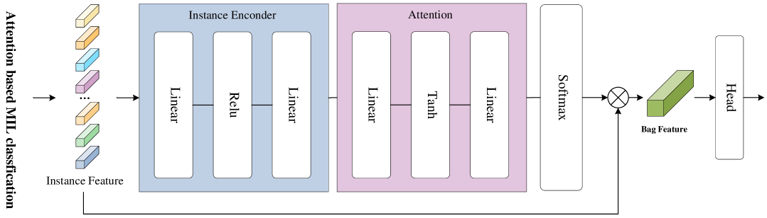
Figure 7: Instance-level to Bag-level Classification Head Block Structure.

$$X=[x_{1},x_{2},\dots,x_{L-1}]\in\mathbb{R}^{B\times(L-1)\times D}$$ (16)

To construct a bag-level representation from these instance-level features, we employ a shared instance encoder that maps each patch feature into a fixed-dimensional latent space. This encoder consists of linear layers followed by non-linear activation functions, such as ReLU, to enhance feature expressiveness and capture underlying pathological patterns. Specifically, instance-level features undergo a linear transformation $f_{\text{enc}}(\cdot)$ for feature mapping:

$$Z_{i}=f_{\text{enc}}(x_{i})=\sigma(W_{\text{enc}}x_{i}+b_{\text{enc}})$$ (17)

where $W_{\text{enc}}$ and $b_{\text{enc}}$ are learnable parameters of the linear transformation, and $\sigma(\cdot)$ represents the ReLU non-linear activation function.

Following instance encoding, an attention mechanism is introduced to learn the significance of each patch in the overall pathology classification task. Specifically, the attention module consists of linear layers and a $\tanh$ activation function to compute the attention scores for each patch:

$$a_{i}=\tanh(W_{\text{att}}Z_{i}+b_{\text{att}})$$ (18)

where $W_{\text{att}}$ and $b_{\text{att}}$ are the parameters of the attention module. These scores are then normalized using a softmax function to ensure they sum to one, allowing the model to focus on the most informative pathological regions:

$$\alpha_{i}=\frac{\exp(a_{i})}{\sum_{j=1}^{L-1}\exp(a_{j})}$$ (19)

The final bag-level feature is obtained through a weighted sum of the instance features, where the learned attention weights $\alpha_{i}$ determine the contribution of each patch to the final decision:

$$Z_{\text{bag}}=\sum_{i=1}^{L-1}\alpha_{i}Z_{i}$$ (20)

This aggregated feature serves as a comprehensive representation of the entire pathology image and is subsequently processed by the classification head for the final diagnostic prediction. The classification head typically consists of a fully connected layer followed by a softmax function:

$$y=\text{softmax}(W_{\text{cls}}Z_{\text{bag}}+b_{\text{cls}})$$ (21)

where $W_{\text{cls}}$ and $b_{\text{cls}}$ are the parameters of the final classification layer, and $y$ represents the predicted class probabilities.

In WSS tasks, relying solely on bag-level predictions is often insufficient, as it tends to capture only the most discriminative regions while ignoring other informative parts of the instance. Therefore, a well-designed instance-level classifier plays a vital role in enhancing model performance. Inspired by  [45], we leverage the attention scores derived from the MIL attention mechanism as soft labels to guide the training of the instance classifier. This design encourages the model to focus not only on the most discriminative instances but also on those that are moderately informative.

After obtaining the final class probability distribution $y$ from the bag-level classification head, we optimize the model using the standard cross-entropy loss between the predicted probability and the ground truth label $y_{\text{true}}$:

$$\mathcal{L}_{\text{bag}}=-\sum_{c=1}^{C}y_{\text{true},c}\log y_{c}$$ (22)

where $C$ is the number of classes, $y_{\text{true},c}$ represents the one-hot encoded ground truth label, and $y_{c}$ is the predicted class probability.

In parallel, the instance classifier is trained using the attention weights as soft supervision. Let $\alpha_{i}$ denote the attention score of the $i$-th instance, and $\hat{y}_{i}$ be the predicted class probability of that instance. The instance-level loss is formulated as:

$$\mathcal{L}_{\text{instance}}=-\sum_{i=1}^{N}\alpha_{i}\log\hat{y}_{i}$$ (23)

The final loss function combines both the bag-level and instance-level objectives:

$$\mathcal{L}_{cls}=\lambda\mathcal{L}_{\text{bag}}+(1-\lambda)\mathcal{L}_{\text{instance}}$$ (24)

where $\lambda$ is a balancing coefficient controlling the trade-off between bag and instance classification.

We employ the Adam optimizer to update the model parameters $\theta$ via backpropagation to minimize the loss:

$$\theta\leftarrow\theta-\eta\frac{\partial\mathcal{L}_{cls}}{\partial\theta}$$ (25)

where $\eta$ is the learning rate. Through iterative optimization, the model improves classification accuracy, enabling effective pathology image recognition.

This attention-based MIL classification head enables the model to effectively highlight critical pathological regions, improving interpretability and facilitating accurate lesion identification even in the absence of pixel-level annotations. The architecture of this classification head is illustrated in Fig. 7, which depicts the instance-to-bag transformation process.

3.6 Cam-seg Model

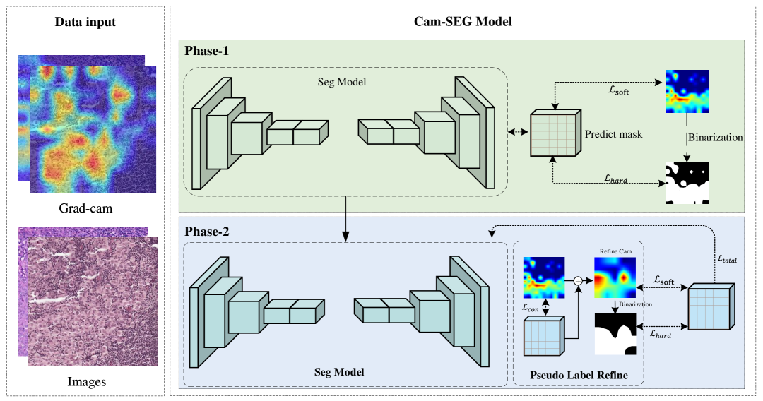
Figure 8: Cam-seg Model Structure.

In traditional two-stage weakly-supervised segmentation tasks, a pseudo-label is typically generated by binarizing the CAM, which is then used as strong supervision to guide the model’s learning. However, these pseudo-labels often contain noise, and such noisy labels may mislead the model, thereby affecting the effectiveness of the training process. To address this issue, this paper proposes a pseudo-label training strategy based on the CAM, aiming to enhance the reliability of the pseudo-labels and thus improve the model’s segmentation performance. The architecture of Cam-seg Model is illustrated in Fig. 8

The model adopts a staged training strategy, using different pseudo-label generation methods at different training stages. In the early stage, pseudo-labels are directly generated from the CAM. In the later stage, the CAM is progressively refined by incorporating the model’s prediction results, ultimately generating more accurate pseudo-labels. Specifically, the training process can be divided into the following stages:

Early stage: In the initial stage of the model, pseudo-labels are directly generated from the CAM, serving as soft pseudo-labels to guide learning. During this phase, the difference between the CAM and the model’s prediction results is measured using the binary cross-entropy (BCE) loss. At this point, the CAM is binarized and used as a hard label, and the differences between the hard label and the model’s predictions are evaluated using the Dice loss and the structure-aware mean Intersection over Union (mIoU) loss. The overall loss function can be expressed as:

$$\mathcal{L}_{total}=\alpha\ \mathcal{L}_{soft}+(1-\alpha)\ \mathcal{L}_{hard}$$ (26)

Mid-to-late stage: As the model training progresses, the CAM is gradually refined by incorporating the model’s prediction results. In regions where the model’s predictions have high confidence, the model’s predictions are prioritized over the CAM labels, thereby reducing the impact of noisy labels. This process helps identify and correct errors or unannotated areas in the CAM. Specifically, the generation of pseudo-labels is performed using confidence-weighted selection. For each pixel, we select the label for that pixel based on a weighted combination of the CAM and the model’s prediction, where the weights are determined by the model’s prediction confidence $\beta$ ($\beta$ > 0.7). Let $y_{cam}$ and $y_{pred}$ represent the labels from the CAM and the model’s predictions, respectively. The confidence-weighted pseudo-label can be expressed as:

$$y_{refined}=\beta\ y_{cam}+(1-\beta)\ y_{pred}$$ (27)

It is worth noting that, to better constrain the model and avoid incorrect pseudo-label corrections, we introduce a consistency loss. For the high-response areas in the CAM, the model is required to maintain high prediction accuracy, ensuring that the model does not overcorrect in these critical regions. This loss function can be expressed as:

$$\mathcal{L}_{\text{con}}=-\frac{1}{N}\sum_{i=1}^{N}\left[y_{i}\log(\hat{y}_{i})+(1-y_{i})\log(1-\hat{y}_{i})\right]$$ (28)

Where $y_{i}$ is the high-response region in the CAM map, and $\hat{y}_{i}$ is the predicted probability value of the model for the corresponding region.

The total loss function of the model in the mid-to-late stage can be expressed as:

$$\mathcal{L}_{total}=\alpha\ \mathcal{L}_{soft}+(1-\alpha)\ \mathcal{L}_{hard}+\mathcal{L}_{con}$$ (29)

Through this training strategy, we are able to introduce stronger structural awareness while ensuring that the model maintains stability in low-confidence areas during the pseudo-label generation process. This allows the model to be effectively trained even in the presence of strong noise, guiding it to perform more accurate segmentation in complex scenarios.

4 Experimental results

4.1 Dataset description

We evaluated our method on both a publicly available dataset (CAMELYON16) and a private dataset (glomerular lesions). Detailed information about each dataset is provided in Tab. 1, some samples are shown in Fig. 9, with the following descriptions:

1) Glomerular Lesions: This dataset consists of 281 PAS-stained kidney biopsy samples collected from Shanxi Provincial People’s Hospital (SPPH) between 2017 and 2020, and 30 kidney biopsy samples collected from the Second Hospital of Shanxi Medical University (SHSXMU) between 2017 and 2019. After glomerular segmentation, a total of 1593 glomeruli containing K-W nodules (positive) and 1660 glomeruli without K-W nodules (negative) were obtained for training classification and lesion detection models. Each glomerular lesion annotation was performed collaboratively by three professional pathologists. Data collection was approved by the ethics committees (SPPH: No.127, SHSXMU: YX.026). For our evaluation, 398 positive images and 414 negative images were selected from the internal dataset.

2) CAMELYON16 Dataset[13]: The CAMELYON16 (Cancer Metastases in Lymph Nodes, 2016) dataset is specifically designed for cancer metastasis detection in pathology images. Provided by the MICCAI 2016 challenge, it has become a widely used benchmark in digital pathology research. The dataset includes 400 whole-slide digital pathology images from 200 breast cancer patients, all stained with hematoxylin and eosin, containing rich tissue details. Each slide image was annotated by pathologists, identifying the regions of cancer metastasis.

It is worth noting that we performed some preprocessing on the CAMELYON16 dataset to facilitate testing our model. Specifically, we downsampled the images using a sliding window approach, dividing each whole-slide image into smaller patches. The label for each patch was assigned based on the patient-level label, ensuring label consistency and accuracy. This preprocessing step not only reduced the computational resources required but also enabled the model to better capture local features in the images.

Table 1: Dataset Information

Category	Attribute	Glomerular	Camelyon16
Dataset Information	Source	private_data	ISBI challenge
	Target	Glomerular spikes	Breast cancer metastases
	Annotation Type	Patient-level & Pixel-level (Only Eval)
	Number of Classes	2 (positive & negative)
	Input Image Size	1100 * 1100
	train:test:val	7:2:1
WSI Distribution	Positive WSIs	212	110
	Negative WSIs	300	160
Patch Statistics	Total (Train/test)	2846/813	13184/3776
	Total (Val)	407	1883
	Positive (Train/test)	1394/398	6410/1832
	Positive (Val)	199	916
	Negative (Train/test)	1452/415	6774/1944
	Negative (Val)	208	967

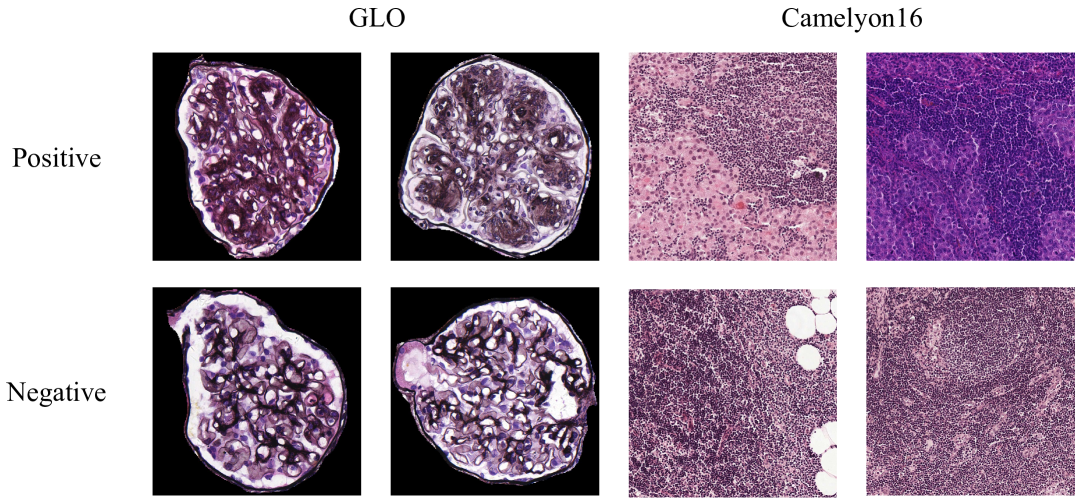
Figure 9: Dataset samples

4.2 Implementation details

Server Configuration: In this study, we conducted experiments on two servers with different configurations. The first server is equipped with six NVIDIA V100 GPUs, while the second server is equipped with a single NVIDIA A6000 GPU. Both servers are running Ubuntu 22.04.3 LTS (x86_64) with the GNU/Linux version 6.2.0-35-generic operating system, and they are configured with CUDA 11.8 drivers to support deep learning acceleration. During the experiments, all input images were standardized to a size of 1100 × 1100 pixels to ensure consistency and uniformity in the data, optimizing both the training and testing efficiency of the model.

Training settings: All models were trained on the training set, and the best accuracy on the validation set was reported. To ensure fair comparison, our training setup follows the benchmark model Vision Mamba[75]. Specifically, we applied data augmentation techniques such as random cropping, random horizontal flipping, label smoothing regularization, mixup, and random erasing. During training, we used ResNet50[21] as a Pre-trained Feature Extraction to extract features for each patch. The optimizer used was AdamW[41], with a momentum of 0.9, a batch size of 12, and a weight decay of 0.05. The model training employed a cosine learning rate scheduler with an initial learning rate of $1\times 10^{-3}$, and the Exponential Moving Average (EMA) training strategy was applied for 300 epochs.

During testing, we applied center cropping to the validation set. To fully leverage the efficient long-sequence modeling capabilities of the FMamba model, we performed fine-tuning after pre-training for 30 epochs, using a long-sequence setting. Specifically, we kept the patch size constant, set the learning rate to $10^{-5}$, and the weight decay to $10^{-8}$. In our experiments, patch size is a critical parameter for the effectiveness of multi-instance learning (MIL). Thus, we treated the patch size as a hyperparameter, adjusting and validating it experimentally to determine the optimal patch size.

In the second stage of the CAM-SEG segmentation task, we employed U-Net as the network backbone. The training parameters were set with an initial learning rate of 0.01, momentum of 0.9, and weight decay rate of 0.0001, with a total of 150 training epochs to obtain the final prediction model. The first 20 epochs were used for preliminary adjustment during training. We analyzed the model’s performance under different loss balancing parameter $\alpha$ settings in the experiments.

Performance metrics: In this study, to comprehensively evaluate the performance of FMaMIL in the weakly-supervised lesion segmentation task, we adopted several internationally recognized evaluation metrics, including Accuracy, F1 Score, Intersection over Union (IoU), Dice coefficient. Additionally, we paid particular attention to the segmentation quality of lesion areas, using probability heatmaps for visualization to further validate the model’s effectiveness in real-world lesion recognition.

Table 2: Comparison of our model with state-of-the-art methods on two datasets.

Type	Method	Seg.Net	Publication	Glomerular lesion				Camelyon16
				Classfication		Segmentation		Classfication		Segmentation
				Acc	AUC	mIoU	Dice	Acc	AUC	mIoU	Dice
WSS	OAA[25]	-	ICCV2019	-	-	0.668	0.712	-	-	0.607	0.652
	Group-WSSS[33]	-	AAAI2021	-	-	0.760	0.842	-	-	0.735	0.754
	Auxsegnet[64]	-	ICCV2021	-	-	0.784	0.736	-	-	0.778	0.804
	L2G[27]	U-Net	CVPR2022	-	-	0.786	0.863	-	-	0.786	0.844
MIL-WSS	DeepAttnMISL[68]	-	MIA2020	-	-	0.706	0.759	-	-	0.714	0.722
	SA-MIL[32]	-	MIA2023	-	-	0.813	0.891	-	-	0.795	0.876
	CLAM-SB[42]	-	Nat. Biomed. Eng2021	0.940	0.952	0.728	0.802	0.873	0.884	0.717	0.734
	CLAM-MB[42]	-		0.951	0.954	0.742	0.815	0.894	0.903	0.725	0.746
	AB-MIL[24]	-	PMLR2018	0.923	0.930	0.721	0.790	0.885	0.889	0.703	0.709
	Trans-MIL[49]	-	NIPS2021	0.963	0.971	0.765	0.847	0.937	0.941	0.768	0.781
Cam-base CA	Resnet34[21]	U-Net	CVPR2016	0.956	0.959	0.655	0.664	0.953	0.960	0.604	0.631
	ConvNeXt[40]	U-Net	CVPR2022	0.988	0.992	0.712	0.776	0.975	0.967	0.727	0.754
Mamba	Vision-mamba[76]	-	ICML 2024	0.946	0.956	0.706	0.715	0.965	0.961	0.731	0.746
	Vision-mamba[76]	U-Net	ICML 2024	0.946	0.956	0.734	0.760	0.965	0.961	0.755	0.763
	MambaMIL[67]	-	MICCAI2024	0.993	0.995	0.831	0.860	0.986	0.989	0.814	0.838
	MambaMIL[67]	U-Net	MICCAI2024	0.993	0.995	0.856	0.879	0.986	0.989	0.846	0.850
	MamMIL[15]	-	BIBM2024	0.990	0.993	0.825	0.861	0.981	0.986	0.807	0.834
	MamMIL[15]	U-Net	BIBM2024	0.990	0.993	0.853	0.873	0.981	0.986	0.843	0.852
Ours	FMaMIL	-	-	0.996	0.998	0.849	0.891	0.993	0.992	0.836	0.884
	FMaMIL	U-Net	-	0.996	0.998	0.870	0.914	0.993	0.992	0.856	0.927
	FMaMIL	Cam-SEG	-	0.996	0.998	0.887	0.934	0.993	0.992	0.869	0.957
FSS	U-Net[47]	-	MICCAI2015	-	-	0.826	0.854	-	-	0.830	0.931
	DeeplabV3+[7]	-	CVPR2017	-	-	0.835	0.860	-	-	0.849	0.923

4.3 Comparison with state-of-the-art methods

In this section, we compare our model with the current state-of-the-art classification and segmentation methods, with the results shown in Tab. 2. All experimental results were tested on the validation set. To assess the model’s performance more objectively and accurately, we invited professional doctors to provide real and detailed annotations for the validation dataset. By examining the experimental results, it is evident that our model shows significant improvement in performance compared to traditional weakly supervised lesion segmentation methods.

Specifically, although WSS methods, represented by MIL-WSSS, have demonstrated advantages to some extent, these methods still face performance bottlenecks due to sequential dependencies and resource limitations. In contrast, our model fully considers the correlations between instances and, by exploring the relationships between instances and bags, extracts pseudo-label features that are more suitable for segmentation tasks. Furthermore, compared to the two-stage approach that uses traditional classification models and utilizes CAM maps as pseudo-labels, our method achieves significant performance improvement. Even when compared to the state-of-the-art method based on Mamba, our model not only achieves higher scores in the classification task but also delivers better performance metrics in the segmentation task. This achievement is attributed to the effective collaboration between the various modules.

In comparison with fully supervised segmentation (FSS) methods,, our model demonstrates unexpected advantages. We conducted an in-depth analysis of the reasons behind this result and found that, although supervised training typically relies on ground truth labels, in the case of medical images, labels are often not fully comprehensive. Some lesion areas may not be precisely annotated, particularly under sparse annotation conditions. These labeling errors can cause the model to overlook certain lesion features, thereby affecting the training outcome. In contrast, our WSS model is more effective at uncovering latent features in the image, thereby enhancing its ability to handle sparse annotation data, ultimately achieving superior model performance.

4.4 Hyper-parameter analysis

In this section, we will examine the impact of key parameters of the FMaMIL model on performance during both the classification and segmentation stages. By systematically analyzing these parameters, our goal is to identify their optimal values, thereby optimizing the model’s performance and maximizing its efficacy.

4.4.1 Hyper-parameters for Different patch Sizes

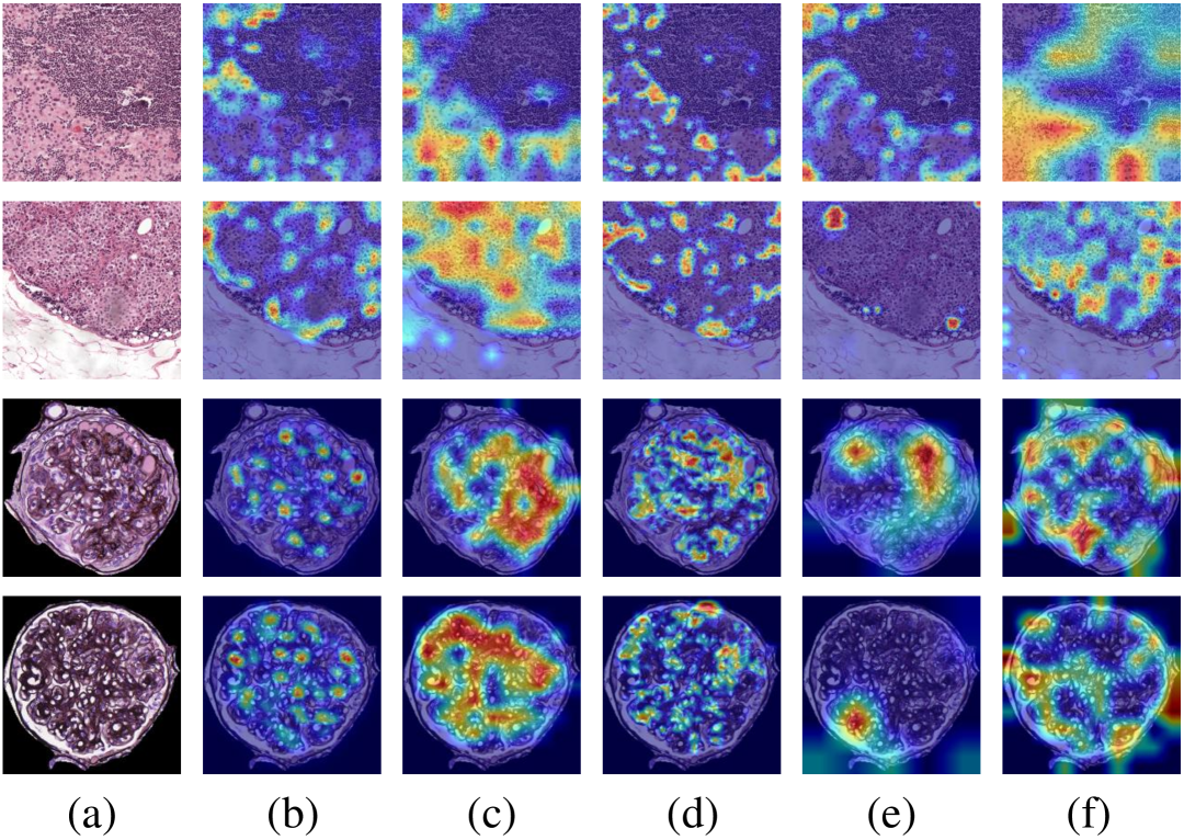
Figure 10: Visualization results of lesion areas with different patch sizes. (a) Original image; (b) Patch size = 50; (c) Patch size = 100 (d) Patch size = 150; (e) Patch size = 200; (f) Patch size = 220;

In our work, input images are divided into patches of varying sizes, and features are extracted from these patches while capturing inter-instance relationships to generate the final model prediction. Selecting an appropriate patch size is crucial for comprehensively understanding image content and extracting detailed features.

In our experiments, we evaluated five different patch sizes: 50×50, 100×100, 150×150, 200×200, and 220×220. For cases where the image dimensions were not evenly divisible, we applied zero-padding to ensure consistency in input size. The experiments were conducted on two datasets to assess the impact of different patch sizes on segmentation and classification tasks, with the results presented in Tab. 3. The findings indicate that a patch size of 100×100 yielded the best performance in both classification and segmentation tasks.

Furthermore, we visualized the Grad-Cam results under different patch sizes, as shown in Fig. 10. The analysis reveals that smaller patches provide finer-grained local information, enabling the model to capture microscopic structures and fine details. However, excessively small patches may lead to the loss of global structural information and significantly increase computational cost. Conversely, larger patches retain more global semantic information, improving the model’s ability to comprehend overall patterns but potentially overlooking critical local details.

Taking the glomerulus dataset as an example, when the patch size was small (e.g., 50×50), many mesangial proliferative regions were not identified, whereas larger patches (e.g., 220×220) resulted in nearly all glomerular regions being misclassified as diseased. In contrast, a patch size of 100×100 produced CAM results that most closely matched the ground truth and achieved the best overall performance. Based on the quantitative experimental results and visualization analysis, we selected 100×100 as the optimal patch size to balance detail preservation and global information integrity.

Table 3: The performance of FMaMIL with different patch sizes.

Patch size	Patch_size	Num_patchs	Glomerular lesion				Camelyon16
			Segmentation		Classification		Segmentation		Classification
			mIoU	Dice	Acc	AUC	mIoU	Dice	Acc	AUC
50	1100	22*22	0.861	0.886	0.986	0.991	0.835	0.903	0.993	0.991
150	1100	8*8(padding)	0.872	0.914	0.993	0.992	0.857	0.914	0.99	0.991
200	1100	6*6(padding)	0.79	0.891	0.991	0.994	0.803	0.868	0.987	0.989
220	1100	5*5	0.771	0.853	0.989	0.99	0.761	0.806	0.984	0.986
FMaMIL(100)	1100	11*11	0.887	0.934	0.996	0.998	0.869	0.957	0.993	0.992

4.4.2 Hyper-parameters selection for classification Loss of balance $\lambda$

In the first-stage classification task, we designed an instance-to-bag classifier that computes both instance-level and bag-level prediction losses. These two losses are balanced using a hyperparameter $\lambda$. We conducted experiments by tuning $\lambda$ within the range of [0.1, 0.9] to determine its optimal value. Since introducing the instance-level loss does not significantly impact the classification performance, we further evaluated its effect on WSS across two datasets. As shown in Fig. 11, the best segmentation performance was achieved when $\lambda=0.2$, indicating an optimal balance between instance-level learning and bag-level supervision.

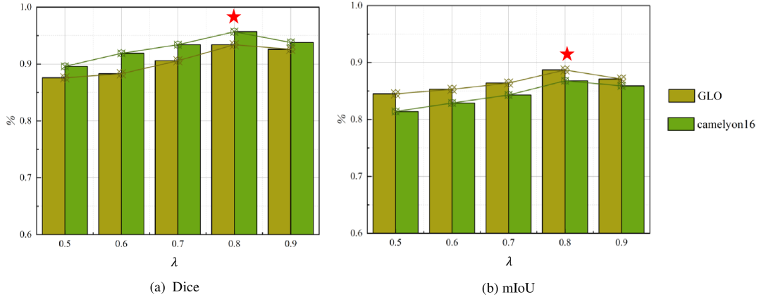
Figure 11: classification Loss of balance $\lambda$

4.4.3 Hyper-parameters for binary threshold $t$

After completing the first-stage classification task, we used Grad-CAM to generate CAMs. During the second-stage supervised segmentation training, we needed to binarize these maps to create masks for computing the hard label update loss. Specifically, when a pixel value in the CAM exceeds the threshold $t$, it is classified as foreground; otherwise, it is classified as background. The choice of threshold $t$ is crucial to the segmentation outcome and directly impacts the performance of the second-stage segmentation. If $t$ is set too high, some lesion regions may be missed, whereas if $t$ is set too low, more irrelevant regions may be identified as lesions, reducing segmentation accuracy.

To determine the optimal threshold $t$, we adjusted its value within the range [0,1] and evaluated the method on two datasets. The experimental results are shown in Fig. 12. The study indicates that when the threshold $t$ is set to 0.5, the second-stage segmentation task achieves the best performance across all datasets.

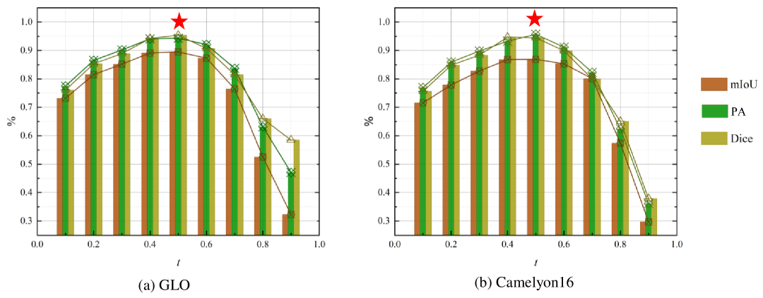
Figure 12: binary threshold $t$

4.4.4 Hyper-parameters for Loss of balance $\alpha$

In the second-stage segmentation task, we employ both soft label loss, computed from the CAM, and hard label loss, derived from the binarized CAM mask. To balance these two loss components, we introduce the loss balance parameter $\alpha$, which controls the relative contribution of the two terms in the overall loss function. Specifically, a higher $\alpha$ increases the influence of the hard label loss, emphasizing more confident regions, while a lower $\alpha$ gives greater weight to the soft label loss, preserving more uncertainty in the learning process.

The choice of $\alpha$ significantly affects the segmentation performance. A large $\alpha$ may lead to over-reliance on the binarized masks, potentially amplifying errors from thresholding, whereas a small $\alpha$ may cause excessive dependence on the soft labels, reducing the model’s ability to refine its predictions.

To determine the optimal $\alpha$, we conduct experiments by varying it within the range [0,1] and evaluate the model performance on two datasets. The results, as shown in Fig. 13, indicate that setting within the range [0,1] to an 0.3 achieves the best segmentation accuracy across datasets.

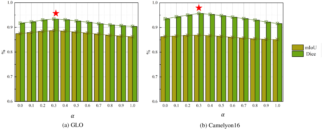
Figure 13: segmentation loss of balance $\alpha$

4.5 Visualization comparison

In pathological image analysis, lesion regions are often characterized by diffuse distributions and indistinct boundaries, which pose significant challenges for accurate localization. To qualitatively assess the effectiveness of our proposed method in lesion localization, we visualize the segmentation results on selected validation samples. As illustrated in Fig. 14 and Fig. 15, we present the intermediate outputs of our method, the final segmentation maps, and comparisons with several state-of-the-art approaches.

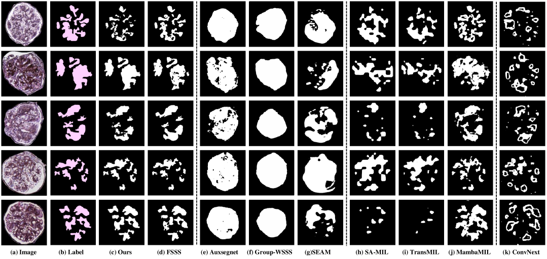
Figure 14: Visualization comparison of lesion segmentation of Glo

The visualizations demonstrate that our method can more precisely localize lesion regions, with the predicted heatmaps exhibiting clearer and more concentrated responses around pathological areas. Compared with conventional MIL methods—where the independence between instances often leads to localization drift and incomplete contextual representation—our approach exhibits superior spatial consistency and semantic relevance. Notably, in the challenging task of K-W nodule recognition, which involves complex lesion morphology and strong background interference, our method maintains robust localization performance, highlighting its strong discriminative capability in spatial regions. It is worth emphasizing that our approach requires only image-level labels during training, yet it achieves lesion predictions that closely align with expert annotations, without any pixel-level supervision.

Furthermore, our method shows promising sensitivity in detecting subtle lesions that are often missed in manual annotations. These results validate the proposed method’s ability to model lesion regions under weak supervision and provide reliable regional information for subsequent quantitative analysis and clinical decision support.

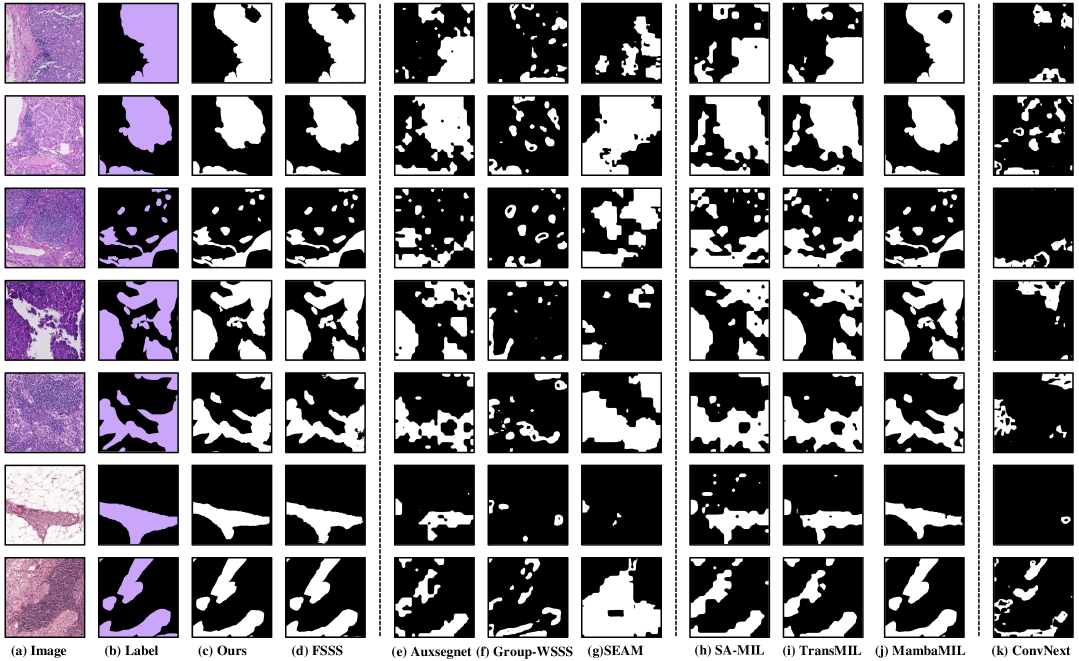
Figure 15: Visualization comparison of lesion segmentation of PatchCamelyon16

4.6 Ablation studies

In this section, we conduct ablation studies to further investigate the impact of each key component on the final segmentation performance and analyze the model’s behavior under different configurations.

4.6.1 Overall Contribution of Classification Stage

We first evaluate the contribution of three core components in the classification stage, including: (1) the bidirectional scanning strategy, (2) the learnable frequency-domain feature encoding, and (3) the dual-supervised multi-instance classification head. The proposed method is systematically validated on two datasets: Glomerular Lesion and Camelyon16. Based on the baseline model Vision-Mamba, we progressively integrate the three components and subsequently perform ablation by individually removing each module from the complete model for comparison. The results are summarized in Tab. 4.

The experimental results clearly demonstrate that all three components play an important role in enhancing the overall model performance. Specifically, the learnable frequency-domain encoding significantly improves feature representation and yields the most notable performance gain. The bidirectional scanning strategy enhances contextual understanding, while the instance-level supervision in the MIL head further refines the quality of the CAMs, leading to more accurate segmentation. Compared to the original baseline, the complete model achieves over 15 percentage points improvement in segmentation performance, which strongly validates the effectiveness and synergy of the proposed components in the weakly supervised lesion segmentation task.

Table 4: Overall Contribution of Classification Stage Components

Methods	Two-Scan	Learn-FFT	MIL-Head	Cam-Seg	Glomerular lesion				Camelyon16
					Classfication		Segmentation		Classfication		Segmentation
					Acc	AUC	mIoU	Dice	Acc	AUC	mIoU	Dice
Baseline(Vision-Mamba)				✓	0.946	0.956	0.734	0.760	0.965	0.961	0.755	0.763
Method-A	✓			✓	0.963	0.970	0.805	0.820	0.978	0.980	0.814	0.835
Method-B		✓		✓	0.982	0.985	0.811	0.855	0.981	0.983	0.839	0.867
Method-C			✓	✓	0.959	0.965	0.763	0.801	0.972	0.974	0.781	0.809
FMaMIL(W/O MIL-head)	✓	✓		✓	0.992	0.995	0.859	0.890	0.990	0.991	0.851	0.891
FMaMIL(W/O FFT)	✓		✓	✓	0.983	0.988	0.843	0.875	0.985	0.987	0.846	0.909
FMaMIL(W/O Twoscan)		✓	✓	✓	0.991	0.995	0.858	0.901	0.988	0.990	0.861	0.927
FMaMIL	✓	✓	✓	✓	0.996	0.998	0.887	0.934	0.993	0.992	0.869	0.957

4.6.2 Effect of Learnable Frequency-Domain Encoding

To further verify the effectiveness of the learnable frequency-domain encoding module, we conducted experiments by separately using high-frequency (>0.8), mid-frequency, and low-frequency (<0.2) components as inputs, aiming to investigate the impact of different frequency bands on lesion recognition and localization. The experimental results are presented in Tab. 5. The results show that incorporating fixed frequency-domain features brings noticeable performance gains compared to not using frequency encoding, indicating that frequency information can enhance the discriminative power of feature representations. Among the fixed frequency bands, mid-frequency features achieve the most significant improvement, suggesting their strong ability to capture lesion boundaries and structural patterns.

In contrast, the learnable frequency-domain encoding allows the model to adaptively select and fuse multi-band frequency information, offering greater flexibility and precision in feature representation and spatial localization. As a result, it achieves the best segmentation performance, further confirming the effectiveness and superiority of this module in the context of weakly supervised lesion segmentation.

Table 5: Effect of Learnable Frequency-Domain Encoding

Methods	Low-freq	Mid-freq	High-freq	Learn-Freq	Glomerular lesion				Camelyon16
					Classfication		Segmentation		Classfication		Segmentation
					ACC	AUC	mIoU	Dice	ACC	AUC	mIoU	Dice
FMaMIL(W/O FFT)					0.983	0.988	0.843	0.875	0.985	0.987	0.846	0.909
Method-D	✓				0.989	0.991	0.861	0.892	0.990	0.991	0.852	0.923
Method-E		✓			0.992	0.994	0.874	0.921	0.991	0.991	0.861	0.945
Method-F			✓		0.981	0.985	0.836	0.854	0.983	0.986	0.838	0.901
FMaMIL				✓	0.996	0.998	0.887	0.934	0.993	0.992	0.869	0.957

4.6.3 Effect of the Scanning Strategy

To evaluate the impact of different scanning strategies on model performance, we investigate the effects of incorporating forward and backward SSM modules, as well as adopting a bidirectional scanning strategy. The experimental results are presented in Tab. 6. The results demonstrate that both forward and backward scanning contribute positively to information propagation and contextual modeling. However, using only a unidirectional row-wise scanning strategy results in inferior performance compared to the bidirectional approach. This indicates that the bidirectional scanning strategy effectively enhances the model’s ability to capture spatial consistency and structural representation, compensating for the spatial information loss inherent in one-dimensional sequences, and providing clearer and more focused activation regions for the classification stage.

Table 6: Effect of the Scanning Strategy

Methods	Forward-SSM	Backward-SSM	Single-Scan	Two-Scan	Glomerular lesion				Camelyon16
					Classfication		Segmentation		Classfication		Segmentation
					ACC	AUC	mIoU	Dice	ACC	AUC	mIoU	Dice
Baseline(W/O B-SSM)	✓		✓		0.925	0.927	0.701	0.713	0.934	0.935	0.702	0.748
Baseline(W/O F-SSM)		✓	✓		0.923	0.926	0.703	0.719	0.931	0.932	0.697	0.741
Baseline(Vision-Mamba)	✓	✓	✓		0.946	0.956	0.734	0.760	0.965	0.961	0.755	0.763
Fmamba(W/O B-SSM)	✓			✓	0.984	0.986	0.854	0.897	0.963	0.965	0.826	0.918
Fmamba(W/O F-SSM)		✓		✓	0.982	0.983	0.856	0.903	0.958	0.960	0.821	0.914
Fmamba	✓	✓		✓	0.996	0.998	0.887	0.934	0.993	0.992	0.869	0.957

4.6.4 Effect of Instance-Level Loss in MIL Head

To investigate the impact of introducing instance-level supervision loss in the multi-instance segmentation framework, we conducted an ablation study by removing the instance-level loss while retaining the image-level classification objective, keeping all other components unchanged. As shown in Tab. 7, the instance-level loss, serving as a fine-grained supervision signal, has limited effect on classification performance but brings significant improvements in the WSS task. This loss effectively enhances the model’s ability to discriminate key instances, thereby improving the quality of the generated CAMs and providing more accurate and focused guidance for the subsequent segmentation module.

Table 7: Effect of Instance-Level Loss in MIL Head

Methods	$\mathcal{L}_{\text{bag}}$	$\mathcal{L}_{\text{instance}}$	Glomerular lesion		Camelyon16
			mIoU	Dice	mIoU	Dice
Method-G	✓		0.865	0.901	0.855	0.921
FMaMIL(ours)	✓	✓	0.887	0.934	0.869	0.957

4.6.5 Overall Contribution in the Segmentation Stage

We comprehensively evaluate the effectiveness of the staged training strategy(STS) and the pseudo label refinement (PLR) module introduced in the second-stage segmentation task. In addition, we analyze the impact of different loss functions on the model performance. The experimental results are presented in Tab 8. When only the hard supervision loss is applied, the model relies solely on the initial coarse pseudo labels for training, resulting in a noticeable decline in segmentation performance. In contrast, introducing the CAM-guided soft supervision loss effectively complements the semantic spatial information of lesion regions and significantly improves segmentation accuracy. The staged training strategy, combined with the PLR module, guides the optimization process in a coarse-to-fine manner. The dynamic refinement of pseudo labels during training helps enhance the quality and stability of the supervision signal. Furthermore, the consistency loss constrains the model’s predictions in high-response CAM regions, improving the stability of responses and the sharpness of lesion boundaries.

Table 8: Overall Contribution and Effect of Loss Functions in the Segmentation Stage

Methods	STS	PLR	$\mathcal{L}_{hard}$	$\mathcal{L}_{soft}$	$\mathcal{L}_{con}$	Glomerular lesion		Camelyon16
						mIoU	Dice	mIoU	Dice
Baseline-A			✓			0.870	0.914	0.856	0.927
Baseline -B				✓		0.872	0.918	0.859	0.934
FMaMIL(w/o PLR)	✓		✓	✓		0.878	0.927	0.862	0.942
FMaMIL(w/o $\mathcal{L}_{con}$)	✓	✓	✓	✓		0.883	0.926	0.865	0.946
FMaMIL(ours)	✓	✓	✓	✓	✓	0.887	0.934	0.869	0.957

5 Discussion

In this study, we propose a two-stage weakly supervised lesion segmentation framework tailored for pathological images. The framework follows a “classification-then-segmentation” paradigm that leverages image-level annotations to enable precise lesion localization and segmentation. In the first stage, we adopt a MIL strategy, where a linear attention module (Mamba) is introduced to capture correlations between instances. Additionally, a learnable frequency-domain encoding module is employed to enhance feature representation, and dual-level supervision—at both the instance and bag levels—is used to generate high-quality and focused CAMs. In the second stage, we utilize a staged training strategy. Specifically, a soft label loss guided by CAMs is used to exploit semantic priors from the classification stage, followed by pseudo label refinement and consistency loss to progressively improve label quality and prediction stability. As a result, our method achieves superior segmentation performance without relying on any pixel-level annotations.

Model interpretability is of great significance in medical image analysis, especially for ensuring clinical reliability and trust. Through comprehensive visualizations and quantitative evaluations, we observe that the predicted segmentation regions closely align with the actual lesion locations, demonstrating that the model effectively attends to clinically relevant areas. Notably, the introduction of instance-level supervision significantly enhances the model’s ability to detect key regions, overcoming the common limitation of conventional classification networks that tend to focus only on the most discriminative regions. Moreover, the learnable frequency-domain encoding and bidirectional scanning strategies jointly improve the model’s perception of complex lesion structures. These modules complement each other by enhancing spatial contextual modeling and capturing detailed frequency information, thereby addressing the limitations of conventional spatial-only approaches and improving both structural interpretability and prediction stability.

While many existing weakly supervised methods directly use coarse CAM maps as segmentation pseudo labels—often resulting in noisy supervision—our framework addresses this from two directions:

• Refining CAM Structure: By enhancing the quality of CAMs, we generate more focused and semantically consistent activation regions, improving the spatial precision of pseudo labels.

• Dynamic Soft Supervision: We introduce soft label losses and iteratively refine pseudo labels using the model’s own predictions, enabling adaptive learning under label noise.

This dual strategy not only improves the reliability of supervision but also highlights the potential of soft supervision in mitigating the adverse effects of noisy labels. Looking ahead, knowledge distillation—particularly in a teacher–student framework—may provide a more robust solution for further reducing bias introduced by imperfect pseudo annotations.

Nevertheless, some limitations remain. Our method still relies on relatively accurate image-level labels, and challenges persist in accurately segmenting lesions with ambiguous boundaries or complex morphologies. Although the Mamba structure improves local dependency modeling, global semantic understanding is still limited. Future work may explore global modeling techniques, such as long-range attention or graph-based methods, to further enhance the model’s holistic perception capabilities.

In summary, the proposed FMaMIL method represents a significant advancement in weakly supervised lesion segmentation by integrating frequency- and spatial-domain information within a MIL framework. It effectively models inter-instance correlations and employs CAM-based soft supervision to enable high-quality segmentation using only image-level labels. Beyond achieving state-of-the-art performance, FMaMIL offers a lightweight and generalizable architecture that addresses key challenges in digital pathology, particularly under annotation-scarce conditions. Looking forward, future work will focus on improving clinical applicability and robustness through domain adaptation and knowledge distillation, paving the way for broader deployment in real-world pathological imaging scenarios.

6 Conclusion

This paper proposes a two-stage weakly supervised lesion segmentation framework, FMaMIL, designed for pathological images. The framework achieves accurate lesion localization and segmentation using only image-level annotations. By effectively integrating frequency-domain and spatial-domain information, and leveraging the long-sequence modeling capabilities of Mamba, the framework captures instance correlations under the MIL paradigm. The high-quality CAMs generated in the classification stage are further utilized to guide the segmentation process. Additionally, we explore the potential of soft label supervision and self-correction mechanisms in mitigating the impact of noisy pseudo labels. Extensive experiments demonstrate the effectiveness and robustness of the proposed method across multiple real-world pathological datasets, providing a practical path toward low-cost and high-precision pathological image analysis. Future work will focus on incorporating knowledge distillation and global semantic modeling to further enhance the generalizability and adaptability of the framework in more complex scenarios, promoting the advancement of weakly supervised lesion segmentation in digital pathology.

References

- Araslanov and Roth [2020] Araslanov, N., Roth, S., 2020. Single-stage semantic segmentation from image labels, in: Proceedings of the IEEE/CVF conference on computer vision and pattern recognition, pp. 4253–4262.
- Bakalo et al. [2021] Bakalo, R., Goldberger, J., Ben-Ari, R., 2021. Weakly and semi supervised detection in medical imaging via deep dual branch net. Neurocomputing 421, 15–25.
- Bearman et al. [2016] Bearman, A., Russakovsky, O., Ferrari, V., Fei-Fei, L., 2016. What’s the point: Semantic segmentation with point supervision, in: European conference on computer vision, Springer. pp. 549–565.
- Campanella et al. [2019] Campanella, G., Hanna, M.G., Geneslaw, L., Miraflor, A., Werneck Krauss Silva, V., Busam, K.J., Brogi, E., Reuter, V.E., Klimstra, D.S., Fuchs, T.J., 2019. Clinical-grade computational pathology using weakly supervised deep learning on whole slide images. Nature medicine 25, 1301–1309.
- Cao et al. [2024] Cao, L., Pan, K., Ren, Y., Lu, R., Zhang, J., 2024. Multi-branch spectral channel attention network for breast cancer histopathology image classification. Electronics 13, 459.
- Chang et al. [2024] Chang, A., Zeng, J., Huang, R., Ni, D., 2024. Em-net: Efficient channel and frequency learning with mamba for 3d medical image segmentation, in: International Conference on Medical Image Computing and Computer-Assisted Intervention, Springer. pp. 266–275.
- Chen et al. [2018] Chen, L.C., Zhu, Y., Papandreou, G., Schroff, F., Adam, H., 2018. Encoder-decoder with atrous separable convolution for semantic image segmentation, in: Proceedings of the European conference on computer vision (ECCV), pp. 801–818.
- Cheplygina et al. [2015] Cheplygina, V., Tax, D.M., Loog, M., 2015. Multiple instance learning with bag dissimilarities. Pattern recognition 48, 264–275.
- Dai et al. [2015] Dai, J., He, K., Sun, J., 2015. Boxsup: Exploiting bounding boxes to supervise convolutional networks for semantic segmentation, in: Proceedings of the IEEE international conference on computer vision, pp. 1635–1643.
- Dietterich et al. [1997] Dietterich, T.G., Lathrop, R.H., Lozano-Pérez, T., 1997. Solving the multiple instance problem with axis-parallel rectangles. Artificial intelligence 89, 31–71.
- Ding et al. [2023] Ding, H., Lu, J., Cai, J., Zhang, Y., Shang, Y., 2023. Slf-unet: Improved unet for brain mri segmentation by combining spatial and low-frequency domain features, in: Computer Graphics International Conference, Springer. pp. 415–426.
- Dong et al. [2018] Dong, N., Kampffmeyer, M., Liang, X., Wang, Z., Dai, W., Xing, E., 2018. Reinforced auto-zoom net: towards accurate and fast breast cancer segmentation in whole-slide images, in: Deep Learning in Medical Image Analysis and Multimodal Learning for Clinical Decision Support: 4th International Workshop, DLMIA 2018, and 8th International Workshop, ML-CDS 2018, Held in Conjunction with MICCAI 2018, Granada, Spain, September 20, 2018, Proceedings 4, Springer. pp. 317–325.
- Ehteshami Bejnordi et al. [2017] Ehteshami Bejnordi, B., Veta, M., Johannes van Diest, P., van Ginneken, B., Karssemeijer, N., Litjens, G., van der Laak, J.A.W.M., , the CAMELYON16 Consortium, 2017. Diagnostic assessment of deep learning algorithms for detection of lymph node metastases in women with breast cancer. JAMA 318, 2199–2210. URL: https://doi.org/10.1001/jama.2017.14585, doi:10.1001/jama.2017.14585, arXiv:https://jamanetwork.com/journals/jama/articlepdf/2665774/jama_ehteshami_bejnordi_2017_oi_170113.pdf.
- Fang et al. [2024a] Fang, H., Huang, S., Tang, W., Huangfu, L., Liu, B., 2024a. Sam-mil: A spatial contextual aware multiple instance learning approach for whole slide image classification, in: Proceedings of the 32nd ACM International Conference on Multimedia, pp. 6083–6092.
- Fang et al. [2024b] Fang, Z., Wang, Y., Zhang, Y., Wang, Z., Zhang, J., Ji, X., Zhang, Y., 2024b. Mammil: Multiple instance learning for whole slide images with state space models, in: 2024 IEEE International Conference on Bioinformatics and Biomedicine (BIBM), IEEE. pp. 3200–3205.
- Feng et al. [2022] Feng, Y., Ma, B., Zhang, J., Zhao, S., Xia, Y., Tao, D., 2022. Fiba: Frequency-injection based backdoor attack in medical image analysis, in: Proceedings of the IEEE/CVF Conference on Computer Vision and Pattern Recognition, pp. 20876–20885.
- Gu and Dao [2023] Gu, A., Dao, T., 2023. Mamba: Linear-time sequence modeling with selective state spaces. arXiv preprint arXiv:2312.00752 .
- Gu et al. [2020] Gu, A., Dao, T., Ermon, S., Rudra, A., Ré, C., 2020. Hippo: Recurrent memory with optimal polynomial projections. Advances in neural information processing systems 33, 1474–1487.
- Han et al. [2022] Han, K., Wang, Y., Chen, H., Chen, X., Guo, J., Liu, Z., Tang, Y., Xiao, A., Xu, C., Xu, Y., et al., 2022. A survey on vision transformer. IEEE transactions on pattern analysis and machine intelligence 45, 87–110.
- Hao et al. [2024] Hao, J., He, L., Hung, K.F., 2024. T-mamba: Frequency-enhanced gated long-range dependency for tooth 3d cbct segmentation. arXiv preprint arXiv:2404.01065 .
- He et al. [2016] He, K., Zhang, X., Ren, S., Sun, J., 2016. Deep residual learning for image recognition, in: Proceedings of the IEEE conference on computer vision and pattern recognition, pp. 770–778.
- Hou et al. [2016] Hou, L., Samaras, D., Kurc, T.M., Gao, Y., Davis, J.E., Saltz, J.H., 2016. Patch-based convolutional neural network for whole slide tissue image classification, in: Proceedings of the IEEE conference on computer vision and pattern recognition, pp. 2424–2433.
- Hu et al. [2024] Hu, Z., Daryakenari, N.A., Shen, Q., Kawaguchi, K., Karniadakis, G.E., 2024. State-space models are accurate and efficient neural operators for dynamical systems. arXiv preprint arXiv:2409.03231 .
- Ilse et al. [2018] Ilse, M., Tomczak, J., Welling, M., 2018. Attention-based deep multiple instance learning, in: International conference on machine learning, PMLR. pp. 2127–2136.
- Jiang et al. [2021] Jiang, P.T., Han, L.H., Hou, Q., Cheng, M.M., Wei, Y., 2021. Online attention accumulation for weakly supervised semantic segmentation. IEEE Transactions on Pattern Analysis and Machine Intelligence 44, 7062–7077.
- Jiang et al. [2019] Jiang, P.T., Hou, Q., Cao, Y., Cheng, M.M., Wei, Y., Xiong, H.K., 2019. Integral object mining via online attention accumulation, in: Proceedings of the IEEE/CVF international conference on computer vision, pp. 2070–2079.
- Jiang et al. [2022] Jiang, P.T., Yang, Y., Hou, Q., Wei, Y., 2022. L2g: A simple local-to-global knowledge transfer framework for weakly supervised semantic segmentation, in: Proceedings of the IEEE/CVF conference on computer vision and pattern recognition, pp. 16886–16896.
- Kanavati et al. [2020] Kanavati, F., Toyokawa, G., Momosaki, S., Rambeau, M., Kozuma, Y., Shoji, F., Yamazaki, K., Takeo, S., Iizuka, O., Tsuneki, M., 2020. Weakly-supervised learning for lung carcinoma classification using deep learning. Scientific reports 10, 9297.
- Khan et al. [2022] Khan, S., Naseer, M., Hayat, M., Zamir, S.W., Khan, F.S., Shah, M., 2022. Transformers in vision: A survey. ACM computing surveys (CSUR) 54, 1–41.
- Lerousseau et al. [2020] Lerousseau, M., Vakalopoulou, M., Classe, M., Adam, J., Battistella, E., Carré, A., Estienne, T., Henry, T., Deutsch, E., Paragios, N., 2020. Weakly supervised multiple instance learning histopathological tumor segmentation, in: Medical Image Computing and Computer Assisted Intervention–MICCAI 2020: 23rd International Conference, Lima, Peru, October 4–8, 2020, Proceedings, Part V 23, Springer. pp. 470–479.
- Li et al. [2025] Li, K., Li, X., Wang, Y., He, Y., Wang, Y., Wang, L., Qiao, Y., 2025. Videomamba: State space model for efficient video understanding, in: European Conference on Computer Vision, Springer. pp. 237–255.
- Li et al. [2023] Li, K., Qian, Z., Han, Y., Eric, I., Chang, C., Wei, B., Lai, M., Liao, J., Fan, Y., Xu, Y., 2023. Weakly supervised histopathology image segmentation with self-attention. Medical Image Analysis 86, 102791.
- Li et al. [2021] Li, X., Zhou, T., Li, J., Zhou, Y., Zhang, Z., 2021. Group-wise semantic mining for weakly supervised semantic segmentation, in: Proceedings of the AAAI conference on artificial intelligence, pp. 1984–1992.
- Liao et al. [2024] Liao, Z., Hu, S., Xie, Y., Xia, Y., 2024. Modeling annotator preference and stochastic annotation error for medical image segmentation. Medical Image Analysis 92, 103028.
- Lin et al. [2018] Lin, H., Chen, H., Dou, Q., Wang, L., Qin, J., Heng, P.A., 2018. Scannet: A fast and dense scanning framework for metastastic breast cancer detection from whole-slide image, in: 2018 IEEE winter conference on applications of computer vision (WACV), IEEE. pp. 539–546.
- Litjens et al. [2017] Litjens, G., Kooi, T., Bejnordi, B.E., Setio, A.A.A., Ciompi, F., Ghafoorian, M., Van Der Laak, J.A., Van Ginneken, B., Sánchez, C.I., 2017. A survey on deep learning in medical image analysis. Medical image analysis 42, 60–88.
- Liu et al. [2021a] Liu, Q., Chen, C., Qin, J., Dou, Q., Heng, P.A., 2021a. Feddg: Federated domain generalization on medical image segmentation via episodic learning in continuous frequency space, in: Proceedings of the IEEE/CVF conference on computer vision and pattern recognition, pp. 1013–1023.
- Liu et al. [2021b] Liu, X., Song, L., Liu, S., Zhang, Y., 2021b. A review of deep-learning-based medical image segmentation methods. Sustainability 13, 1224.
- Liu et al. [2024] Liu, Y., Tian, Y., Zhao, Y., Yu, H., Xie, L., Wang, Y., Ye, Q., Liu, Y., 2024. Vmamba: Visual state space model. CoRR abs/2401.10166. URL: https://doi.org/10.48550/arXiv.2401.10166.
- Liu et al. [2022] Liu, Z., Mao, H., Wu, C.Y., Feichtenhofer, C., Darrell, T., Xie, S., 2022. A convnet for the 2020s, in: Proceedings of the IEEE/CVF conference on computer vision and pattern recognition, pp. 11976–11986.
- Loshchilov [2017] Loshchilov, I., 2017. Decoupled weight decay regularization. arXiv preprint arXiv:1711.05101 .
- Lu et al. [2021] Lu, M.Y., Williamson, D.F., Chen, T.Y., Chen, R.J., Barbieri, M., Mahmood, F., 2021. Data-efficient and weakly supervised computational pathology on whole-slide images. Nature biomedical engineering 5, 555–570.
- Maron and Lozano-Pérez [1997] Maron, O., Lozano-Pérez, T., 1997. A framework for multiple-instance learning. Advances in neural information processing systems 10.
- Qu et al. [2024] Qu, H., Ning, L., An, R., Fan, W., Derr, T., Liu, H., Xu, X., Li, Q., 2024. A survey of mamba. arXiv preprint arXiv:2408.01129 .
- Qu et al. [2022] Qu, L., Wang, M., Song, Z., et al., 2022. Bi-directional weakly supervised knowledge distillation for whole slide image classification. Advances in Neural Information Processing Systems 35, 15368–15381.
- Quellec et al. [2017] Quellec, G., Cazuguel, G., Cochener, B., Lamard, M., 2017. Multiple-instance learning for medical image and video analysis. IEEE reviews in biomedical engineering 10, 213–234.
- Ronneberger et al. [2015] Ronneberger, O., Fischer, P., Brox, T., 2015. U-net: Convolutional networks for biomedical image segmentation, in: Medical image computing and computer-assisted intervention–MICCAI 2015: 18th international conference, Munich, Germany, October 5-9, 2015, proceedings, part III 18, Springer. pp. 234–241.
- Ruan et al. [2025] Ruan, J., Gao, J., Xie, M., Xiang, S., 2025. Learning multi-axis representation in frequency domain for medical image segmentation. Machine Learning 114, 10.
- Shao et al. [2021] Shao, Z., Bian, H., Chen, Y., Wang, Y., Zhang, J., Ji, X., et al., 2021. Transmil: Transformer based correlated multiple instance learning for whole slide image classification. Advances in neural information processing systems 34, 2136–2147.
- Vaswani [2017] Vaswani, A., 2017. Attention is all you need. Advances in Neural Information Processing Systems .
- Waleffe et al. [2024] Waleffe, R., Byeon, W., Riach, D., Norick, B., Korthikanti, V., Dao, T., Gu, A., Hatamizadeh, A., Singh, S., Narayanan, D., et al., 2024. An empirical study of mamba-based language models. arXiv preprint arXiv:2406.07887 .
- Wang et al. [2017] Wang, L., Lu, H., Wang, Y., Feng, M., Wang, D., Yin, B., Ruan, X., 2017. Learning to detect salient objects with image-level supervision, in: Proceedings of the IEEE conference on computer vision and pattern recognition, pp. 136–145.
- Wang et al. [2021] Wang, S., Li, C., Wang, R., Liu, Z., Wang, M., Tan, H., Wu, Y., Liu, X., Sun, H., Yang, R., et al., 2021. Annotation-efficient deep learning for automatic medical image segmentation. Nature communications 12, 5915.
- Wang et al. [2019a] Wang, S., Yang, D.M., Rong, R., Zhan, X., Xiao, G., 2019a. Pathology image analysis using segmentation deep learning algorithms. The American journal of pathology 189, 1686–1698.
- Wang et al. [2019b] Wang, X., Chen, H., Gan, C., Lin, H., Dou, Q., Tsougenis, E., Huang, Q., Cai, M., Heng, P.A., 2019b. Weakly supervised deep learning for whole slide lung cancer image analysis. IEEE transactions on cybernetics 50, 3950–3962.
- Wang et al. [2020] Wang, X., Tang, F., Chen, H., Luo, L., Tang, Z., Ran, A.R., Cheung, C.Y., Heng, P.A., 2020. Ud-mil: uncertainty-driven deep multiple instance learning for oct image classification. IEEE journal of biomedical and health informatics 24, 3431–3442.
- Wang et al. [2024] Wang, X., Wang, S., Ding, Y., Li, Y., Wu, W., Rong, Y., Kong, W., Huang, J., Li, S., Yang, H., et al., 2024. State space model for new-generation network alternative to transformers: A survey. arXiv preprint arXiv:2404.09516 .
- Wang et al. [2018] Wang, X., Yan, Y., Tang, P., Bai, X., Liu, W., 2018. Revisiting multiple instance neural networks. Pattern recognition 74, 15–24.
- Wei et al. [2017] Wei, Y., Feng, J., Liang, X., Cheng, M.M., Zhao, Y., Yan, S., 2017. Object region mining with adversarial erasing: A simple classification to semantic segmentation approach, in: Proceedings of the IEEE conference on computer vision and pattern recognition, pp. 1568–1576.
- Wu et al. [2024] Wu, Y., Ye, X., Yang, K., Li, J., Li, X., 2024. Dupl: Dual student with trustworthy progressive learning for robust weakly supervised semantic segmentation, in: Proceedings of the IEEE/CVF Conference on Computer Vision and Pattern Recognition, pp. 3534–3543.
- Xiao et al. [2015] Xiao, T., Xia, T., Yang, Y., Huang, C., Wang, X., 2015. Learning from massive noisy labeled data for image classification, in: Proceedings of the IEEE conference on computer vision and pattern recognition, pp. 2691–2699.
- Xu et al. [2024] Xu, H., Usuyama, N., Bagga, J., Zhang, S., Rao, R., Naumann, T., Wong, C., Gero, Z., González, J., Gu, Y., et al., 2024. A whole-slide foundation model for digital pathology from real-world data. Nature , 1–8.
- Xu et al. [2020] Xu, K., Qin, M., Sun, F., Wang, Y., Chen, Y.K., Ren, F., 2020. Learning in the frequency domain, in: Proceedings of the IEEE/CVF conference on computer vision and pattern recognition, pp. 1740–1749.
- Xu et al. [2021] Xu, L., Ouyang, W., Bennamoun, M., Boussaid, F., Sohel, F., Xu, D., 2021. Leveraging auxiliary tasks with affinity learning for weakly supervised semantic segmentation, in: Proceedings of the IEEE/CVF international conference on computer vision, pp. 6984–6993.
- Xu et al. [2017] Xu, Y., Jia, Z., Wang, L.B., Ai, Y., Zhang, F., Lai, M., Chang, E.I.C., 2017. Large scale tissue histopathology image classification, segmentation, and visualization via deep convolutional activation features. BMC bioinformatics 18, 1–17.
- Xu et al. [2014] Xu, Y., Zhu, J.Y., Eric, I., Chang, C., Lai, M., Tu, Z., 2014. Weakly supervised histopathology cancer image segmentation and classification. Medical image analysis 18, 591–604.
- Yang et al. [2024] Yang, S., Wang, Y., Chen, H., 2024. Mambamil: Enhancing long sequence modeling with sequence reordering in computational pathology, in: International Conference on Medical Image Computing and Computer-Assisted Intervention, Springer. pp. 296–306.
- Yao et al. [2020] Yao, J., Zhu, X., Jonnagaddala, J., Hawkins, N., Huang, J., 2020. Whole slide images based cancer survival prediction using attention guided deep multiple instance learning networks. Medical image analysis 65, 101789.
- Yue and Li [2024] Yue, Y., Li, Z., 2024. Medmamba: Vision mamba for medical image classification. arXiv preprint arXiv:2403.03849 .
- Zhang et al. [2025] Zhang, Y., Li, H., Sun, Y., Zheng, S., Zhu, C., Yang, L., 2025. Attention-challenging multiple instance learning for whole slide image classification, in: European Conference on Computer Vision, Springer. pp. 125–143.
- Zhang et al. [2024] Zhang, Y., Zhang, X., Wang, J., Yang, Y., Peng, T., Tong, C., 2024. Mamba2mil: State space duality based multiple instance learning for computational pathology. arXiv preprint arXiv:2408.15032 .
- Zheng et al. [2024] Zheng, Y., Sharma, H., Betke, M., Beane, J., Kolachalama, V.B., 2024. Fouriermil: Fourier filtering-based multiple instance learning for whole slide image analysis. bioRxiv , 2024–08.
- Zhou et al. [2016] Zhou, B., Khosla, A., Lapedriza, A., Oliva, A., Torralba, A., 2016. Learning deep features for discriminative localization, in: Proceedings of the IEEE conference on computer vision and pattern recognition, pp. 2921–2929.
- Zhou et al. [2024] Zhou, Z., He, A., Wu, Y., Yao, R., Xie, X., Li, T., 2024. Spatial-frequency dual progressive attention network for medical image segmentation. arXiv preprint arXiv:2406.07952 .
- Zhu et al. [2024a] Zhu, L., Liao, B., Zhang, Q., Wang, X., Liu, W., Wang, X., 2024a. Vision mamba: Efficient visual representation learning with bidirectional state space model. arXiv preprint arXiv:2401.09417 .
- Zhu et al. [2024b] Zhu, L., Liao, B., Zhang, Q., Wang, X., Liu, W., Wang, X., 2024b. Vision mamba: Efficient visual representation learning with bidirectional state space model. arXiv preprint arXiv:2401.09417 .