Superconducting photocurrents induced by structured electromagnetic radiation

Abstract

We develop a phenomenological theory describing the interaction of superconducting condensate with a Bessel beam of twisted light characterized by a nonzero angular momentum $m$. Starting from the time-dependent Ginzburg-Landau model with the complex relaxation time we calculate the spatial profiles of dc photoinduced currents and magnetic fields as well as the second harmonic response. The photocurrents and magnetic fileds are shown to be determined both by the helicity of light and its orbital momentum $m$. Analyzing the half-space and thin film geometries we discuss possible experimental tests aimed to probe the superconducting photocurrents and magnetic fields.

I Introduction

Recent progress in the study of a variety of optoelectronic phenomena and their applications triggered the interest to the dissipationless photocurrents which can be generated in systems with superconducting elements. The key distinctive feature of these photocurrents carried by the Cooper pairs is that they can persist even after the switching off the electromagnetic pulse responsible for the current generation. Such persistent current becomes possible due to the photoinduced superconducting vortices penetrating the system acquiring, thus, the angular momentum from the incident electromagnetic wave [1, 2]. The primary angular momentum of the incident light pulse can originate either from its circular polarization or from a nontrivial orbital structure of the light beam. The transfer of the angular momentum for the case of circularly polarized radiation can be illustrated even for the case of the plane wave and this phenomenon is well known as the inverse Faraday effect [3]. In the context of superconducting materials the mechanisms of this effect have been recently discussed in [4, 5]. Turning to the case of the electromagnetic radiation with a nonzero orbital momentum we need to consider the so-called twisted light which can be realized in Bessel or Laguerre-Gaussian beams [6, 7, 8, 9] (see also [10] for review). Advances in the development and manipulation of the structured light beams have significantly expanded the possibilities for studying light-matter interactions. The propagation and scattering of beams in various media are of particular interest as the study of these phenomena opens the possibility of deeper understanding of the physics of light-matter interaction (see, e.g., [11, 12]). Note that the study of photogalvanic effects in media irradiated by structured light is also of practical interest, particularly, for the development of compact devices that enhance optical communication and data processing by utilizing the orbital angular momentum of light [13].

Considering the nonlinear electrodynamics of these beams we will focus only on the second-order nonlinear effects as they define the rectification phenomena. Typical second-order nonlinear effects occurring in metals, semiconductors, or plasma during interaction with radiation include the inverse Faraday effect [3, 15, 14], the Gaponov-Miller force [16, 15, 14, 17], ac Hall effect [18], and related photon drag phenomenon [19, 20, 21, 22, 23, 24, 25]. Detailed study of these effects for the particular case of structured light (i.e. light beams) illuminating semiconducting samples have been recently presented in Refs. [26, 27].

Turning now to the case of superconductors we have to note that for the plane waves the above second-order effects have been recently addressed in a number of works based mainly on the time - dependent Ginzburg - Landau theory. In particular, above the critical temperature $T_{c}$ in the fluctuating regime the second order nonlinearities have been studied in Refs. [28, 29, 30, 31]. Below $T_{c}$ the mechanisms responsible for the inverse Faraday effect and photon drag of Cooper pairs have been revealed in Refs. [32, 4]. These mechanisms originate from the time - dependent modulation of the superfluid density caused by the charge imbalance potential $\tilde{\phi}$ induced by the field of the incident electromagnetic wave. As a result, the supercurrent contains the term proportional to the product of the superfluid velocity and charge imbalance potential generating, thus, the second - order response.

The goal of the present work is to generalize the studies [32, 4] to the case of structured light illuminating the superconducting condensate focusing on the particular case of Bessel beams. The primary calculation tool in our work is the time-dependent Ginzburg-Landau (TDGL) formalism. The key ingredient which allows to study the second - order nonlinearities within this formalism is the imaginary part of the relaxation constant which is defined by the electron-hole asymmetry [33, 34]. Note that accounting for the second order nonlinear response of the condensate and related rectification effects distinguishes our consideration from the previous studies of interaction of structured light with superconducting systems [35, 36]. Following the approach developed in [32] we calculate the magnitudes of the charge imbalance potential $\tilde{\phi}$ and order parameter modulation $\Delta_{1}$ in superconductor. We calculate the induced photocurrent and compensating Meissner currents both at zero frequency and the second harmonic, and finally obtain the photoinduced magnetic field profiles which can be measured by a certain local probe techniques [see Fig. 1]. Based on our calculations for a superconducting half-space, the magnetic field at the interface at the center of the beam can be estimated as follows: $B_{z}\sim\nu\kappa^{2}\lambda\xi\frac{B_{0}^{2}}{H_{\text{cm}}}$, where $\nu$ is the ratio between imaginary and real parts of the relaxation constant $\Gamma$ in TDGL model, $1/\kappa=c/(\omega\sin\theta)$ is the beam length scale in the sample plane, $\lambda$ is the London penetration depth, $\xi$ is the superconducting coherence length, $B_{0}$ is the characteristic amplitude of the magnetic field in the beam and $H_{cm}$ is the thermodynamic critical field of the superconductor. The total photoinduced magnetic field has two contributions: the one of orbital origin proportional to the $m$ value and, thus, antisymmetric under the substitution $m\rightarrow-m$, and the one associated with the polarization rotation related, therefore, to the inverse Faraday effect. It is important to note that the photocurrents and resulting magnetic fields can be strengthened in thin film geometry in the factor $(\lambda/d)^{2}$, if the film thickness $d$ is less than the London penetration depth $\lambda$. Thus, the use of thin superconducting films in the experimental setup can facilitate the observation of the above effects.

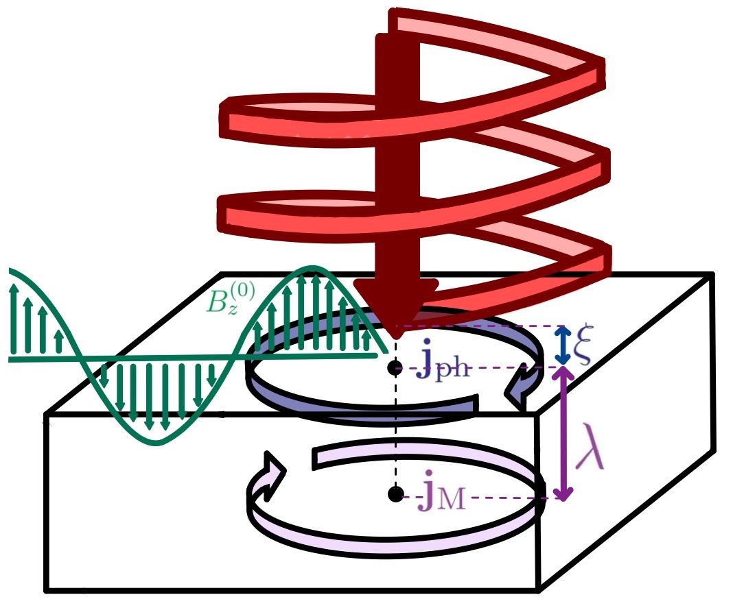
Figure 1: Schematic experimental setup for detection of photocurrents induced by structured light. The figure shows a beam incident on a superconductor, the photoinduced current $\mathbf{j}_{\text{ph}}$ flowing at the depth $\sim\xi$, and the screening Meissner current $\mathbf{j}_{\text{M}}$ flowing at the depth $\sim\lambda$.

The remainder of the paper is organized as follows. In Section II we give the basic equations of the time-dependent Ginzburg-Landau theory. In Section III we discuss the auxilliary problem of photon drag for the case of plane waves with mixed polarization. In Sections IV and V we present the calculations of photocurrents and related magnetic fields for the Bessel beam interacting with superconducting half-space and thin film, respectively. Finally, the results are summarized in Sec. VI.

II Basic equations

In our study of the second-order nonlinear electrodynamic response of superconductor we follow the approach adopted previously in [4, 32, 31], namely, the time-dependent Ginzburg-Landau (TDGL) theory with a complex relaxation constant $\Gamma$:

$$-\Gamma\left(\hbar\partial_{t}-2ie\phi\right)\Delta=\\ -aT_{c}\epsilon\Delta+b|\Delta|^{2}\Delta+aT_{c}\xi_{0}^{2}\left(-i\mathbf{\nabla}+\frac{2\pi}{\Phi_{0}}\mathbf{A}\right)^{2}\Delta$$ (1)

where $\Gamma=\frac{\pi a}{8}+i\gamma$, $\Phi_{0}=\pi\hbar c/e$ ($e>0$). The imaginary part of the relaxation constant is known to reflect a small electron-hole asymmetry. Assuming that the external field is sufficiently weak, we adopt a perturbation expansion for the order parameter in the form $\Delta=(\Delta_{0}+\Delta_{1})e^{i\chi}$, where $\Delta_{0}^{2}=aT_{c}\epsilon/b$ is the equilibrium order parameter in the absence of the external field, and $\epsilon=(T_{c}-T)/T_{c}$. Corrections to the order parameter amplitude $\Delta_{1}$, and phase $\chi$ are assumed to be proportional to the amplitude of the electromagnetic wave.

Though the above model has a rather restricted range of validity and assumes a gapless superconducting state, such consideration is known to provide instructive insights for a great variety of dynamic phenomena. Microscopic derivation of the TDGL model has been previously obtained for two possible scenarios when the gap suppresion is caused either by paramagnetic impurities or by the presence of rather strong electron-phonon relaxation (see [34, 38] for review).

Taking a single Fourier harmonic of the incident electromagnetic wave ($\propto e^{-i\omega t}$) one can write the second-order response of the superconductor through the complex amplitudes of the correction to the gap $\Delta_{1}$ and the superfluid velocity $\mathbf{v}_{s}$:

$$\mathbf{j}_{\text{ph}}=\mathbf{j}_{\text{ph}}^{(0)}+\mathbf{j}_{\text{ph}}^{(2\omega)}=-2e\Delta_{0}\operatorname{Re}[\left(\Delta^{*}_{1}+\Delta_{1}e^{-2i\omega t}\right)\mathbf{v}_{s}]$$ (2)

The equation for the correction $\Delta_{1}$ reads (see Appendix A for details):

$$-\nabla^{2}\Delta_{1}+q_{1}^{2}\Delta_{1}=\frac{2e\tau\nu\Delta_{0}}{\hbar\xi^{2}}\tilde{\phi},$$ (3)

where $q_{1}^{2}\equiv\frac{2-i\omega\tau}{\xi^{2}}$, $\xi^{2}=\xi_{0}^{2}/\epsilon$, $\tau=\pi\hbar/8T_{c}\epsilon$, and the parameter $\nu=8\gamma/\pi a$ is the ratio of the imaginary and real parts of $\Gamma$. Here we introduce a charge imbalance potential $\tilde{\phi}=\phi-\mu_{p}$, which is known to characterize the difference between the chemical potential of normal quasiparticles in a superconductor and the chemical potential of Cooper pairs $\mu_{p}=(\hbar/2e)\partial\chi/\partial t$ [39]. The equation for the charge imbalance potential $\tilde{\phi}(\mathbf{r})$ takes the form (see Appendix A for details):

$$\nabla^{2}\tilde{\phi}=q_{2}^{2}\tilde{\phi},$$ (4)

where $q_{2}^{2}\equiv\frac{1}{l_{E}^{2}}-\frac{i\omega\tau}{\xi^{2}}=\frac{\lambda^{2}}{l_{E}^{2}\lambda_{\text{eff}}^{2}}$, $l_{E}^{2}=\hbar\sigma_{n}/\pi ae^{2}\Delta_{0}^{2}$, $\lambda^{2}=\hbar^{2}c^{2}/32\pi aT_{c}\xi_{0}^{2}e^{2}\Delta_{0}^{2}$, $\frac{1}{\lambda_{\text{eff}}^{2}}=\frac{1}{\lambda^{2}}\left(1-i\omega\tau\frac{l_{E}^{2}}{\xi^{2}}\right)$. Note that for further estimates we will take $l_{E}=\xi/\sqrt{5.79}$ keeping in mind the parameters of the TDGL model derived for the case of strong electron-phonon relaxation (see [40]).

The superfluid velocity in the expression (2) can be obtained from the Maxwell’s equations. In the linear approximation the magnetic and electric fields inside superconductor ($\mathbf{H}^{(i)}$ and $\mathbf{E}^{(i)}$) satisfy the following equations derived in Appendix B:

$$\Delta\mathbf{H}^{(i)}=\frac{1}{\lambda_{\text{eff}}^{2}}\mathbf{H}^{(i)}\ ,$$ (5)

$$\operatorname{curl}\mathbf{H}^{(i)}=\frac{ic}{\omega}\left(\frac{1}{\lambda_{\text{eff}}^{2}}\mathbf{E}^{(i)}+\frac{1}{\lambda^{2}}\nabla\tilde{\phi}\right)\ .$$ (6)

The superfluid velocity can be expressed through the field $\mathbf{E}^{(i)}$:

$$\mathbf{v}_{s}=-\frac{4ieaT_{c}\xi_{0}^{2}}{\omega\hbar^{2}}\left(\mathbf{E}^{(i)}+\nabla\tilde{\phi}\right)\approx-\frac{4ieaT_{c}\xi_{0}^{2}}{\omega\hbar^{2}}\mathbf{E}^{(i)}\approx\\ -\frac{4eaT_{c}\xi_{0}^{2}\lambda^{2}_{\text{eff}}}{c\hbar^{2}}\operatorname{curl}\mathbf{H}^{(i)}\ .$$ (7)

Here, the term $\nabla\tilde{\phi}$ appears to be small in the parameter $\omega/\sigma_{n}$ and can be omitted. Indeed, the use of the Leontovich boundary condition for the tangential components of the fields at the surface of metal assumes that the normal to the surface electric field component is small in the above ratio $\omega/\sigma_{n}$. It is this normal field component which generates the gradient of the charge imbalance potential inside the superconductor and, thus, its value is also determined by the small factor $\omega/\sigma_{n}$. The upper limit for the frequencies considered in our work is obviously determined by the superconducting gap value and, thus, should be in the THz frequency range ($\omega\lesssim 10^{12}s^{-1}$). These values are certainly much less than typical values of conductivity $\sigma_{n}\sim 10^{18}s^{-1}$.

III Auxilliary problem. Photon drag for mixed polarization of the incident wave

Keeping in mind that further consideration of the structured light requires to take account of the coexistence of the waves of different polarization it is convenient first to generalize the description of Ref. [32] for the case of photon drag arising in the presence of electromagnetic wave with both P- and S- polarizations (the corresponding orientations of electric and magnetic fields are shown in Fig.2). This auxilliary problem should illustrate how these polarizations mix on the second order nonlinearity in the superconductor response and create the dc current. Thus, we consider the electromagnetic wave incident on a superconductor surface consisting of the mixture of P- and S- polarized parts. For P-polarization the complex amplitudes of incident and reflected waves (omitting the factor $e^{-i\omega t}$) are given by the expressions (the unspecified components are equal to zero, see Fig.2):

$$\begin{cases}E_{x}^{(e)}=E_{0}\cos\theta e^{ik_{x}x}\left(e^{ik_{z}z}-r_{\parallel}e^{-ik_{z}z}\right)\ ,\\ B_{y}^{(e)}=B_{0}e^{ik_{x}x}\left(e^{ik_{z}z}+r_{\parallel}e^{-ik_{z}z}\right)\ ,\\ E_{z}^{(e)}=-E_{0}\sin\theta e^{ik_{x}x}\left(e^{ik_{z}z}+r_{\parallel}e^{-ik_{z}z}\right)\ .\end{cases}$$ (8)

For S-polarization these amplitudes take the form (see Fig.2):

$$\begin{cases}B_{x}^{(e)}=B_{0}\cos\theta e^{ik_{x}x}\left(e^{ik_{z}z}+r_{\perp}e^{-ik_{z}z}\right)\\ E_{y}^{(e)}=-E_{0}e^{ik_{x}x}\left(e^{ik_{z}z}-r_{\perp}e^{-ik_{z}z}\right)\\ B_{z}^{(e)}=-B_{0}\sin\theta e^{ik_{x}x}\left(e^{ik_{z}z}-r_{\perp}e^{-ik_{z}z}\right)\end{cases}$$ (9)

Hereafter indices $(e)$ and $(i)$ stand for the external and internal fields. Next we consider the superposition of two polarizations and introduce the polarization unit vector corresponding to the magnetic field direction:

$$\mathbf{e}_{\text{H}}=\alpha\mathbf{e}_{\text{H}}^{\parallel}+\beta\mathbf{e}_{\text{H}}^{\perp}\ ,$$ (10)

where

$$\begin{cases}\mathbf{e}_{\text{H}}^{\parallel}=(0,1,0)^{T},\\ \mathbf{e}_{\text{H}}^{\perp}=(\cos\theta,0,-\sin\theta)^{T}.\end{cases}$$ (11)

The complex coefficients $\alpha$ and $\beta$) are the amplitudes of the P- and S- polarization contributions to the fields, $|\alpha|^{2}+|\beta|^{2}=1$.

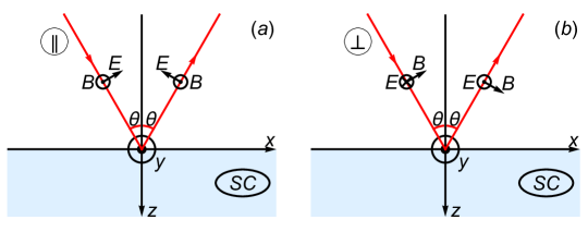
Figure 2: Incident and reflected wave structure for P-polarization (a) and for S-polarization (b).

In order to calculate the reflection coefficients, we neglect the term $\nabla\tilde{\phi}$ in equation (6) assuming the limit of $\omega\ll\sigma_{n}$ and $l_{E}\ll\lambda$, which looks reasonable for a II-type superconductor:

$$\operatorname{curl}\mathbf{H}^{(i)}=\frac{ic}{\omega\lambda_{\text{eff}}^{2}}\mathbf{E}^{(i)}.$$ (12)

Taking into account the expressions (8) and (9), we obtain the reflection coefficients $r_{\parallel}$ and $r_{\perp}$ for P- and S- polarizations, correspondingly (see [41]):

$$r_{\parallel}=\frac{1+i\frac{\omega\lambda_{\text{eff}}}{c\cos{\theta}}}{1-i\frac{\omega\lambda_{\text{eff}}}{c\cos{\theta}}}\ ,$$ (13)

$$r_{\perp}=\frac{1+i\frac{\omega\cos{\theta}\lambda_{\text{eff}}}{c}}{1-i\frac{\omega\cos{\theta}\lambda_{\text{eff}}}{c}}.$$ (14)

Eq. (5) gives us the solution for the magnetic field inside the superconductor. Exploiting the continuity of the tangential component of the magnetic field we obtain

$$H^{(i)}_{y}=(1+r_{\parallel})\alpha B_{0}e^{ik_{x}x-z/\lambda_{\text{eff}}}$$ (15)

for P-polarization and

$$H^{(i)}_{x}=(1+r_{\perp})\beta B_{0}\cos\theta e^{ik_{x}x-z/\lambda_{\text{eff}}}.$$ (16)

for S-polarization. Hereafter we put the reflection coefficients $r_{\parallel}=1$ and $r_{\perp}=1$ assuming that $\omega|\lambda_{\text{eff}}|/c\ll 1$ and taking $\theta$ not very close to $\pi/2$. Therefore, the $z$-component $H^{(i)}_{z}\propto(1-r_{\parallel})$ is omitted.

To compute the light-induced current, we need the correction to the absolute value of the order parameter $\Delta_{1}(\mathbf{r})$ (see Eq.(2)). Note that since the $z$-component of the electric field for S-polarization is zero (see Fig. 2), this polarization does not contribute to $\tilde{\phi}$ and $\Delta_{1}$: $\tilde{\phi}=\Delta_{1}=0$. Thus, we need to calculate the quantity $\Delta_{1}(\mathbf{r})$ only for P-polarization.

Disregarding a very thin surface layer (of the thickness of Thomas-Fermi screening length $\lambda_{\text{TF}}\ll\xi$) accumulating the oscillating surface charge we can choose the boundary condition for the charge imbalance potential in the form

$$\partial\tilde{\phi}/\partial z|_{z=0}=-E_{z}^{(i)}|_{z=0}=-\frac{c}{4\pi\sigma}\partial H_{y}^{(i)}/\partial x|_{z=0}\ .$$ (17)

The corresponding solution of Eq. (4) reads

$$\tilde{\phi}=\alpha\frac{i\omega\sin\theta B_{0}}{2\pi\sigma_{n}q_{2}}e^{ik_{x}x}e^{-q_{2}z}\ .$$ (18)

Using the above expressions and the boundary condition $\partial\Delta_{1}/\partial z|_{z=0}=0$ we find the solution of Eq. (3):

$$\Delta_{1}=-\alpha\frac{i\omega e\tau\nu\Delta_{0}B_{0}\sin\theta}{\pi\hbar\sigma_{n}\xi^{2}(q_{1}^{2}-q_{2}^{2})}e^{ik_{x}x}\left(\frac{e^{-q_{1}z}}{q_{1}}-\frac{e^{-q_{2}z}}{q_{2}}\right).$$ (19)

Neglecting the small corrections in the parameter $\omega\lambda/c$ we get the expression

$$\operatorname{curl}\mathbf{H}^{(i)}\approx\begin{pmatrix}-\partial H^{(i)}_{y}/\partial z\\ \partial H^{(i)}_{x}/\partial z\\ \partial H^{(i)}_{y}/\partial x\end{pmatrix}=\frac{2B_{0}}{\lambda_{\text{eff}}}\begin{pmatrix}\alpha\\ -\beta\cos\theta\\ i\alpha\sin\theta\lambda_{\text{eff}}\omega/c\end{pmatrix}\ ,$$ (20)

which allows us to find the superfluid velocity according to the Eq. (7). Here the column vectors are written in the Cartezian coordinate system.

Finally, in the presence of both polarizations we get the rectified current density vector at zero frequency $\mathbf{I}^{(0)}_{\text{ph}}=-2e\Delta_{0}\operatorname{Re}\int_{0}^{+\infty}dz\Delta_{1}^{*}\mathbf{v_{s}}$:

$$\mathbf{I}^{(0)}_{\text{ph}}=\frac{\nu}{\sqrt{2}\pi}\frac{\xi}{\tau}\frac{B_{0}^{2}\sin{\theta}}{H_{cm}}\frac{\omega\tau}{1+\omega^{2}\tau^{2}\eta^{2}}\times\\ \operatorname{Re}\left[i\frac{\sqrt{1+i\omega\tau\eta}}{2-i\omega\tau}\begin{pmatrix}|\alpha|^{2}\\ -\alpha\beta^{*}\cos{\theta}\\ -i|\alpha|^{2}\sin\theta(\lambda\omega/c\sqrt{1+i\omega\tau\eta})\end{pmatrix}\right]\ ,$$ (21)

where the parameter $\eta=l_{E}^{2}/\xi^{2}$ characterizes the ratio between the superconducting coherence length and the electric field penetration depth. Note that in the limit $\alpha=1,\beta=0$ the Eq.(21) gives us the result for P-polarization obtained in [32]. The $y$-component of the Eq. (21) proportional to $\alpha\beta^{*}$ is responsible for the mixing of polarizations due to second-order nonlinearity: the wave with S-polarization induces the in-plane screening current while the wave with P-polarization modulates the superconducting density through the effects of the charge imbalance potential. It is this mechanism of interaction between two polarizations which we plan to exploit in the following consideration of light beams electrodynamics. Note briefly that the above photocurrent density should generate additional Meissner current and superconductor phase distributions at zero frequency. These currents will guarantee the absence of a dc magnetic field deep inside the superconductor and compensate the nonzero divergence of the $z$-component of photocurrent. We will discuss the details of this compensation when considering the electrodynamics of beams below.

IV Interaction of a Bessel beam of twisted light with a superconducting half-space

As a next step, we develop the description of the interaction of the Bessel beam with the bulk superconductor. Bessel beam is defined as a superposition of plane waves with wave vectors lying on a cone with a fixed angle to the propagation axis. The magnetic field in the Bessel beam takes the form [10]:

$$\mathbf{H}^{(e)}=B_{0}e^{ik_{z}z}\int\frac{d^{2}\vec{k}_{\parallel}}{(2\pi)^{2}}e^{i\vec{k}_{\parallel}\vec{\rho}}a_{\kappa m}(k_{\parallel})\mathbf{e}_{\text{H}}\ ,$$ (22)

where

$$a_{\kappa m}(k_{\parallel})=\frac{2\pi}{\kappa}i^{-m}\delta(k_{\parallel}-\kappa)e^{im\varphi_{k}}\ ,$$ (23)

$\mathbf{e}_{H}(\varphi_{k})=\alpha\mathbf{e}^{\parallel}_{H}(\varphi_{k})+\beta\mathbf{e}^{\perp}_{H}(\varphi_{k})$ is a mixed polarization unity vector, $\varphi_{k}$ is an angle in the momentum space, and $\vec{\rho}=(\rho\cos{\varphi},\rho\sin{\varphi})^{T}$. Details of the calculation of the integral (22) are provided in Appendix C. The incident wave can be written as follows:

$$\mathbf{H}^{(e)}=\begin{pmatrix}H_{\rho}^{(e)}\\ H_{\varphi}^{(e)}\\ H_{z}^{(e)}\end{pmatrix}=\frac{B_{0}}{2}e^{ik_{z}z+im\varphi}\times\\ \begin{pmatrix}-J_{m+1}(\kappa\rho)o_{-}-J_{m-1}(\kappa\rho)o_{+}\\ iJ_{m+1}(\kappa\rho)o_{-}-iJ_{m-1}(\kappa\rho)o_{+}\\ -2\beta\sin\theta J_{m}(\kappa\rho)\end{pmatrix},$$ (24)

where $o_{\pm}=\alpha\pm i\beta\cos\theta$ and $\kappa=k\sin\theta$. The parameter $m$ here can be viewed as a topological quantity which defines the beam’s angular momentum. Taking into account the reflected wave and continuity of the tangetial component of the magnetic field at the boundary and assuming $r_{\parallel},r_{\perp}\approx 1$, we can neglect the $z$-component of the magnetic field and obtain the field inside the superconductor half-space in the form:

$$\mathbf{H}^{(i)}=B_{0}e^{-z/\lambda_{\text{eff}}+im\varphi}\times\\ \begin{pmatrix}-J_{m+1}(\kappa\rho)o_{-}-J_{m-1}(\kappa\rho)o_{+}\\ iJ_{m+1}(\kappa\rho)o_{-}-iJ_{m-1}(\kappa\rho)o_{+}\\ 0\end{pmatrix}\ .$$ (25)

Using the boundary conditions at $z=0$

$$\partial\tilde{\phi}/\partial z|_{z=0}=-E_{z}^{(i)}|_{z=0}=-\frac{c}{4\pi\sigma}(\operatorname{curl}\mathbf{H}^{(i)})_{z}|_{z=0}=\\ -\frac{c}{4\pi\sigma}2i\alpha\kappa B_{0}e^{im\varphi}J_{m}(\kappa\rho),$$ (26)

$$\partial\Delta_{1}/\partial z|_{z=0}=0$$ (27)

we solve the equations (4), (3) and obtain the expressions for $\tilde{\phi}(\mathbf{r})$ and $\Delta_{1}(\mathbf{r})$:

$$\tilde{\phi}=\frac{i\alpha\omega\sin\theta B_{0}}{2\pi\sigma_{n}q_{2}}e^{-q_{2}z+im\varphi}J_{m}(\kappa\rho)\ ,$$ (28)

$$\Delta_{1}=-\frac{i\alpha\omega e\tau\nu\Delta_{0}B_{0}\sin\theta}{\pi\hbar\sigma_{n}\xi^{2}(q_{1}^{2}-q_{2}^{2})}\times\\ \left(\frac{e^{-q_{1}z}}{q_{1}}-\frac{e^{-q_{2}z}}{q_{2}}\right)e^{im\varphi}J_{m}(\kappa\rho).$$ (29)

In order to obtain the superfluid velocity, we have to calculate $\operatorname{curl}\mathbf{H}^{(i)}$ and after that use the formula (7). The main terms of the in-plane components of $\operatorname{curl}\mathbf{H}^{(i)}$ come from derivatives $\partial/\partial z$, other derivatives are parametrically smaller and can be neglected:

$$\operatorname{curl}\mathbf{H}^{(i)}\approx\begin{pmatrix}-\partial H_{\varphi}^{(i)}/\partial z\\ \partial H_{\rho}^{(i)}/\partial z\\ \frac{1}{\rho}\partial(\rho H_{\varphi}^{(i)})/\partial\rho-\frac{1}{\rho}\partial H_{\rho}^{(i)}/\partial\varphi\end{pmatrix}=\\ \frac{B_{0}}{\lambda_{\text{eff}}}e^{-z/\lambda_{\text{eff}}+im\varphi}\begin{pmatrix}iJ_{m+1}(\kappa\rho)o_{-}-iJ_{m-1}(\kappa\rho)o_{+}\\ J_{m+1}(\kappa\rho)o_{-}+J_{m-1}(\kappa\rho)o_{+}\\ 2i\alpha J_{m}(\kappa\rho)\kappa\lambda_{\text{eff}}\end{pmatrix}\ .$$ (30)

General expression for the photoinduced current of the second order in the incident wave amplitude has two harmonics:

$$\mathbf{j}_{\text{ph}}=\mathbf{j}_{\text{ph}}^{(0)}+\mathbf{j}_{\text{ph}}^{(2\omega)}=\frac{8e^{2}aT_{c}\xi_{0}^{2}\Delta_{0}}{c\hbar^{2}}\times\\ \operatorname{Re}\left[\left(\Delta^{*}_{1}+\Delta_{1}e^{-2i\omega t}\right)\lambda^{2}_{\text{eff}}\operatorname{curl}\mathbf{H}^{(i)}\right]\ ,$$ (31)

where $\mathbf{j}_{\text{ph}}^{(0)}=-2e\Delta_{0}\operatorname{Re}\left[\Delta_{1}^{*}\mathbf{v}_{s}\right]$ is the zero-frequency current, $\mathbf{j}_{\text{ph}}^{(2\omega)}=-2e\Delta_{0}\operatorname{Re}\left[\Delta_{1}\mathbf{v}_{s}e^{-2i\omega}\right]$ is the second-harmonic response which oscillates at $2\omega$ frequency, and $\mathbf{v}_{s}$ is given by (7).

The resulting photoinduced current at zero frequency takes the form:

$$\mathbf{j}^{(0)}_{\text{ph}}=\frac{\nu B_{0}^{2}\omega\sin\theta}{\sqrt{2}H_{cm}\lambda\xi l_{E}^{2}}\operatorname{Re}\Bigg{[}\frac{\lambda^{*}_{\text{eff}}f_{\text{ph}}(z)}{q_{1}q_{2}(q_{1}+q_{2})}\times\\ \begin{pmatrix}i_{1}(\rho)+i_{2}(\rho)\\ i_{3}(\rho)+i_{4}(\rho)\\ i_{5}(\rho)\end{pmatrix}\Bigg{]}\ ,$$ (32)

where

$$f_{\text{ph}}(z)=\frac{1}{q_{1}^{-1}-q_{2}^{-1}}\left(\frac{e^{-q_{1}z}}{q_{1}}-\frac{e^{-q_{2}z}}{q_{2}}\right)\ ,$$ (33)

$i_{1}(\rho)=-|\alpha|^{2}J_{m}(\kappa\rho)\frac{\partial J_{m}(\kappa\rho)}{\kappa\partial\rho}$, $i_{2}(\rho)=\frac{im\alpha\beta^{*}\cos\theta}{\kappa\rho}J^{2}_{m}(\kappa\rho)$, $i_{3}(\rho)=\alpha\beta^{*}\cos\theta J_{m}(\kappa\rho)\frac{\partial J_{m}(\kappa\rho)}{\kappa\partial\rho}$, $i_{4}(\rho)=\frac{im|\alpha|^{2}}{\kappa\rho}J^{2}_{m}(\kappa\rho)$, $i_{5}(\rho)=i|\alpha|^{2}J_{m}^{2}(\kappa\rho)\kappa\lambda^{*}_{\text{eff}}$.

The expression (32) contains five contributions to the total current density ($i_{1-5}$):

• The term $i_{1}$ is proportional to $\frac{\partial J^{2}_{m}(\kappa\rho)}{\kappa\partial\rho}$ is a ponderomotive force, since it is determined by the gradient of the intensity of the electromagnetic wave.

• The term $i_{3}$ can be viewed as a manifestation of the inverse Faraday effect and depends on the helicity of the incident wave. The magnetization distribution can be defined as $\mathbf{M}\propto J^{2}_{m}(\kappa\rho)$ and the term $J_{m}(\kappa\rho)\frac{\partial J_{m}(\kappa\rho)}{\kappa\partial\rho}$ arises, thus, from the current density $c\operatorname{curl}\mathbf{M}$.

• Both $i_{2}$ and $i_{4}$ terms originate from the photon drag effect. The presence of both radial and azimuthal components indicates the spirality of the drag current.

• The $z$-component $i_{5}$ is a consequence of the momentum transfer due to the reflection of the incident wave and can be also explained by the photon drag effect.

Omitting the calculation details we also give here the expression describing the second harmonic response:

$$\mathbf{j}^{(2\omega)}_{\text{ph}}=\frac{\nu B_{0}^{2}\omega\sin\theta}{\sqrt{2}H_{cm}\lambda\xi l_{E}^{2}}\operatorname{Re}\Bigg{[}e^{-2i\omega t+2im\varphi}\frac{\lambda_{\text{eff}}f_{\text{ph}}(z)}{q_{1}q_{2}(q_{1}+q_{2})}\times\\ \begin{pmatrix}i^{(2\omega)}_{1}(\rho)+i^{(2\omega)}_{2}(\rho)\\ i^{(2\omega)}_{3}(\rho)+i^{(2\omega)}_{4}(\rho)\\ i^{(2\omega)}_{5}(\rho)\end{pmatrix}\Bigg{]}\ ,$$ (34)

where $i^{(2\omega)}_{1}(\rho)=\alpha^{2}J_{m}(\kappa\rho)\frac{\partial J_{m}(\kappa\rho)}{\kappa\partial\rho}$, $i^{(2\omega)}_{2}(\rho)=\frac{im\alpha\beta\cos\theta}{\kappa\rho}J^{2}_{m}(\kappa\rho)$, $i^{(2\omega)}_{3}(\rho)=-\alpha\beta\cos\theta J_{m}(\kappa\rho)\frac{\partial J_{m}(\kappa\rho)}{\kappa\partial\rho}$, $i^{(2\omega)}_{4}=\frac{im\alpha^{2}}{\kappa\rho}J^{2}_{m}(\kappa\rho)$, $i^{(2\omega)}_{5}=\alpha^{2}J_{m}^{2}(\kappa\rho)\kappa\lambda_{\text{eff}}$.

The photoinduced dc current calculated above should be obviously screened by the Meissner currents so that to provide the cancellation of the dc magnetic field inside supeconducting halfspace at the distance of the order of the London penetration depth $\lambda$ from the surface. Another important point is that dc photocurrents (32) have nozero divergence which must be compensated by a certain current which would provide the possibility to avoid the time – dependent charge accumulation. In a non-superconducting systems, this issue is known to be resolved by introducing the inhomogeneous distribution of the chemical potential responsible for the diffusion currents compensating the photoinduced ones [26]. In the case of superconductor an adequate compensating mechanism arises from the inhomogeneous distribution of the superconducting phase. To calculate all these screening and compensating currents as well as the related magnetic field we consider standard London electrodynamics described by the following equations for the vector potential $\mathbf{A}^{(0)}$:

$$\begin{cases}\operatorname{curl}\operatorname{curl}\mathbf{A}^{(0)}=\frac{4\pi}{c}\left(\mathbf{j}_{\text{M}}^{(0)}+\mathbf{j}_{\text{ph}}^{(0)}\right),\\ \frac{4\pi\lambda^{2}}{c}\mathbf{j}_{\text{M}}^{(0)}=-\mathbf{A}^{(0)}+\frac{\hbar c}{2e}\nabla\chi^{(0)}\ ,\end{cases}$$ (35)

where $\operatorname{curl}\mathbf{A}^{(0)}=\mathbf{B}^{(0)}$, $\mathbf{j}^{(0)}_{\text{ph}}$, $\mathbf{j}^{(0)}_{\text{M}}$ and $\chi^{(0)}$ are zero-frequency quantities.

From the system (35) we obtain general equations describing the fields inside and outside the superconductor:

$$\Delta\mathbf{A}^{(0)}-\operatorname{grad}\operatorname{div}\mathbf{A}^{(0)}-\frac{1}{\lambda^{2}}\mathbf{A}^{(0)}=-\frac{4\pi}{c}\mathbf{j}^{(0)}_{\text{ph}}-\frac{\hbar c}{2e\lambda^{2}}\nabla\chi^{(0)}$$ (36)

for $z>0$, and

$$\Delta\mathbf{A}^{(0)}-\operatorname{grad}\operatorname{div}\mathbf{A}^{(0)}=0$$ (37)

for $z<0$.

We will solve the problem of calculation of the screening currents in two steps. First, we will calculate the divergence-free component of the current $j^{(0)}_{\text{M},\varphi}$; this component is essential to determine the vertical component of the magnetic field $B^{(0)}_{z}$. Second, we will calculate the component of the current $j^{(0)}_{\text{M},\rho}$, which obviously has a non-zero divergence. This divergence is compensated by the vertical component $j^{(0)}_{\text{M},z}$, driven by the phase gradient $\partial\chi^{(0)}/\partial z$. Using these expressions, we will calculate the in-plain magnetic field component $B^{(0)}_{\varphi}$.

The first step: calculation of $j^{(0)}_{\text{M},\varphi}$ and $B_{z}^{(0)}$.

Let us consider the $\varphi$-component of the photoinduced current defined by the expression (32) :

$$j^{(0)}_{\text{ph},\varphi}(\rho,z)=\operatorname{Re}\left[f_{\text{ph}}(z)j^{(c,0)}_{\text{ph},\varphi}(\rho,0)\right]\ ,$$ (38)

where

$$j^{(c,0)}_{\text{ph},\varphi}(\rho,0)=\frac{\nu B_{0}^{2}\omega\sin\theta}{\sqrt{2}H_{\text{cm}}l_{E}^{2}\xi\lambda}\frac{\lambda^{*}_{\text{eff}}}{q_{1}q_{2}(q_{1}+q_{2})}(i_{3}(\rho)+i_{4}(\rho))\ .$$ (39)

Note that due to the cylindrical symmetry the equation (36) for the $\varphi$-component of $\mathbf{A}$ can be written as:

$$\begin{cases}(\Delta\mathbf{A}^{(0)})_{\varphi}-\frac{1}{\lambda^{2}}A^{(0)}_{\varphi}=-\frac{4\pi}{c}j^{(0)}_{\text{ph},\varphi}(\rho,z)\ ,z>0\ ,\\ (\Delta\mathbf{A}^{(0)})_{\varphi}=0\ ,z<0\ .\end{cases}$$ (40)

Accounting for the difference between the length scales of the solution in the plane $(xy)$ and along the $z$ direction ($1/\kappa\gg\xi,\lambda$) we can search the vector potential in the form:

$$A^{(0)}_{\varphi}=-\frac{4\pi\lambda^{2}}{c}\operatorname{Re}\left[f_{\text{M}}(z)j^{(c,0)}_{\text{ph},\varphi}(\rho,0)\right]\ .$$ (41)

Taking now the equations

$$\begin{cases}\frac{\partial^{2}A^{(0)}_{\varphi}}{\partial z^{2}}-\frac{1}{\lambda^{2}}A^{(0)}_{\varphi}=-\frac{4\pi}{c}j^{(0)}_{\text{ph},\varphi}(\rho,z)\ ,z>0\ ,\\ \frac{\partial^{2}A^{(0)}_{\varphi}}{\partial z^{2}}=0\ ,z<0\ ,\end{cases}$$ (42)

and assuming the continuity of the function $A^{(0)}_{\varphi}$ and its derivative at $z=0$ we find the solution which does not grow at $z=\pm\infty$:

$$f_{\text{M}}(z)=\frac{\lambda^{-2}}{q_{2}-q_{1}}\left(\frac{q_{2}e^{-q_{1}z}}{q_{1}^{2}-\lambda^{-2}}-\frac{q_{1}e^{-q_{2}z}}{q_{2}^{2}-\lambda^{-2}}\right)-\\ -\frac{\lambda^{-1}}{q_{1}^{-1}-q_{2}^{-1}}\left(\frac{1}{q_{1}^{2}-\lambda^{-2}}-\frac{1}{q_{2}^{2}-\lambda^{-2}}\right)e^{-z/\lambda}\ .$$ (43)

The spatial profiles of the resulting photoinduced and Meissner currents are shown in Fig. 3.

It is useful to note here that due to simple relation

$$\int_{0}^{+\infty}dzf_{\text{ph}}(z)=-\int_{0}^{+\infty}dzf_{\text{M}}(z)=\frac{q_{1}+q_{2}}{q_{1}q_{2}}.$$ (44)

the resulting magnetic moment of the total current is equal to zero:

$$M_{z}=\frac{1}{c}\int_{0}^{\infty}\int_{0}^{\infty}dzd\rho\,\pi\rho^{2}\left(j_{\text{ph},\varphi}^{(0)}+j_{\text{M},\varphi}^{(0)}\right)=0\ .$$ (45)

Thus, magnetic moments of the photoinduced and Meissner current exactly compensate each other.

Keeping in mind possible experiments on photon drag effects it looks reasonable to focus on the calculation of magnetic field components which can be measured by different local probe or magnetooptics techniques [42, 44, 43, 45]. We start from the analysis of the profiles of the $B_{z}$ component of the magnetic field determined by the $\varphi$ component of the vector potential

$$B^{(0)}_{z}=\frac{1}{\rho}\frac{\partial(\rho A^{(0)}_{\varphi})}{\partial\rho}=-\frac{4\pi\lambda^{2}}{c}f_{\text{M}}(z)\frac{\partial(\rho j^{(0)}_{\text{ph},\varphi}(\rho,0))}{\rho\partial\rho}\ .$$ (46)

The typical spatial distributions of the $z$-component of the magnetic field are shown in Fig.4. Note that within the above approximation $1/\kappa\gg\xi,\lambda$ the value $B^{(0)}_{z}(0,0)$ appears to be nonzero only for $m=0,\pm 1$. The frequency dependence of the magnetic field in the center of the beam is shown in Fig.5. This plot can be also viewed as a temperature dependence of the field since the frequency enters the related expressions through the factor $\omega\tau$, where $\tau\sim 1/(T_{c}-T)$. Experimentally temperature dependences are probably more accessible for measurements than the frequency ones as the latter assume the tuning of the frequency of the incident wave.

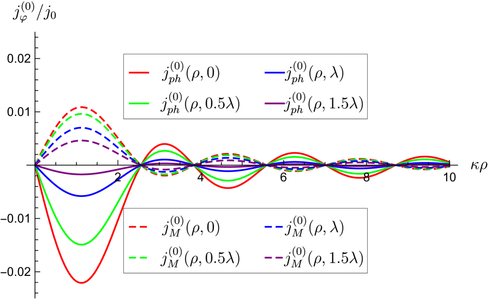
Figure 3: Typical photoinduced and Meissner current profiles. Here we put $\lambda/\xi=2$, $l_{E}/\xi=1/\sqrt{5.79}$, $\omega\tau=1$, $\alpha=1/\sqrt{2},\beta=i/\sqrt{2},m=1,\theta=\pi/4$, $j_{0}=\nu B_{0}^{2}\omega\sin{\theta}/\sqrt{2}H_{\text{cm}}$.

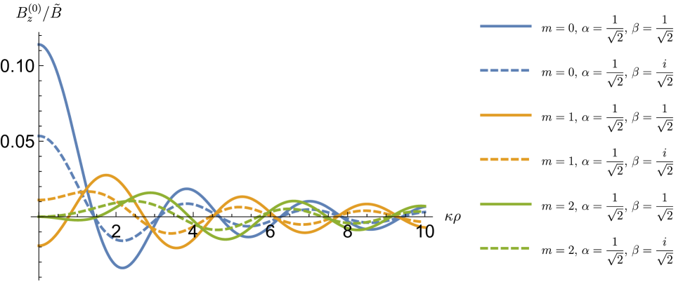
Figure 4: Magnetic field profiles $B_{z}(\rho)$. Here we put $\lambda/\xi=2$, $l_{E}/\xi=1/\sqrt{5.79}$, $\omega\tau=1$, $\tilde{B}=4\pi\nu B_{0}^{2}/\sqrt{2}H_{\text{cm}}$. The values $\alpha,\beta,m$ are shown in the legend.

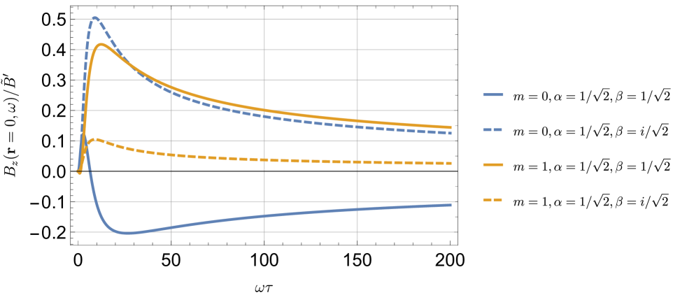
Figure 5: Frequency dependence of magnetic field $B_{z}(\omega)$. Here we put $\lambda/\xi=2$, $l_{E}/\xi=1/\sqrt{5.79}$, $\omega\tau=1$, $\tilde{B}^{\prime}=4\pi\nu(\lambda/c\tau)^{2}B_{0}^{2}/\sqrt{2}H_{\text{cm}}$. The values $\alpha,\beta,m$ are shown in the legend. At $\omega\tau\to\infty$ the magnetic field decays as $\propto 1/\sqrt{\omega\tau}$.

In order to obtain the nonzero value of $B^{(0)}_{z}(0,0)$ for other $m$ numbers, we need to consider the magnetic field up to the first order corrections in the parameter $\kappa\lambda$. Using the Fourier-Bessel transform

$$A^{(0)}_{\varphi}(k_{\rho}) =\int_{0}^{+\infty}A^{(0)}_{\varphi}(\rho)J_{1}(k_{\rho}\rho)\rho d\rho\ ,$$ (47)

$$j_{\text{ph},\varphi}^{(0)}(k_{\rho}) =\int_{0}^{+\infty}j_{\text{ph},\varphi}^{(0)}(\rho)J_{1}(k_{\rho}\rho)\rho d\rho\ .$$ (48)

in Eqs. (40), (42) we get the equations:

$$\begin{cases}\frac{\partial^{2}A^{(0)}_{\varphi}}{\partial z^{2}}-\left(k_{\rho}^{2}+\frac{1}{\lambda^{2}}\right)A^{(0)}_{\varphi}=-\frac{4\pi}{c}f_{\text{ph}}(z)j^{(0)}_{\text{ph},\varphi}(k_{\rho},0)\ ,z>0\ ,\\ \frac{\partial^{2}A^{(0)}_{\varphi}}{\partial z^{2}}-k_{\rho}^{2}A^{(0)}_{\varphi}=0\ ,z<0\ .\end{cases}$$ (49)

In the first order of the perturbation theory in the parameter $\kappa\lambda$ we obtain a nonzero magnetic field in the center for $|m|>1$:

$$B^{(0)}_{z}(0,0)=-\frac{2\sqrt{2}\pi\nu B_{0}^{2}\kappa^{3}\lambda^{2}}{H_{cm}\xi l_{E}^{2}}\times\\ \operatorname{Re}\left[\frac{\lambda^{*}_{\text{eff}}(1+(q_{1}+q_{2})\lambda)}{q_{1}q_{2}(q_{1}+q_{2})(1+q_{1}\lambda)(1+q_{2}\lambda)}C\right]\approx\\ -2\sqrt{2}\pi\frac{\nu B_{0}^{2}\kappa^{3}\lambda^{2}}{H_{cm}\xi l_{E}^{2}}\operatorname{Re}\Biggl{[}\frac{\lambda^{*}_{\text{eff}}}{q_{1}^{2}q_{2}^{2}}C\Biggr{]}\ ,$$ (50)

where

$$C=\int_{0}^{+\infty}\int_{0}^{+\infty}\rho d\rho\frac{k_{\rho}^{3}}{\kappa^{2}}dk_{\rho}J_{1}(k_{\rho}\rho)(i_{3}(\rho)+i_{4}(\rho))=\\ =\frac{32(im|\alpha|^{2}-(3\pi/2)\alpha\beta^{*}\cos\theta)}{\pi(4m^{2}-1)(4m^{2}-9)}\ .$$ (51)

is a complex number of the order unity.

Note that considering the generalization of the above perturbation theory for the full $B^{(0)}_{z}(\rho,0)$ profiles (not only for $\rho=0$) we need to take account of small corrections to the reflection coefficients.

The second step: calculation of $j^{(0)}_{\text{M},\rho},j^{(0)}_{\text{M},z}$ and $B^{(0)}_{\varphi}$.

Let us now consider the vector-potential component induced by the radial and vertical ($z$) components of the photocurrent and take the expansion of this quantity in the small parameter $\kappa\lambda$: $\mathbf{A}^{(0)}_{\text{div}}=\mathbf{A}^{(0)}_{0}+\mathbf{a}^{(0)}$, where $\mathbf{A}^{(0)}_{0}=(A^{(0)}_{0},0,0)^{T}$ being the main term and $\mathbf{a}^{(0)}$ being the higher-order correction. In the leading approximation in the parameter $\kappa\lambda$ the corresponding equations take the form

$$\begin{cases}\frac{\partial^{2}A^{(0)}_{0}}{\partial z^{2}}-\frac{1}{\lambda^{2}}A^{(0)}_{0}=-\frac{4\pi}{c}j^{(0)}_{\text{ph},\rho}(\rho,z)\ ,z>0\ ,\\ \frac{\partial^{2}A^{(0)}_{0}}{\partial z^{2}}=0\ .\end{cases}$$ (52)

The solution of Eq. (52) is similar to Eq. (41):

$$A^{(0)}_{0}=-\frac{4\pi\lambda^{2}}{c}\operatorname{Re}\left[f_{\text{M}}(z)j^{(c,0)}_{\text{ph},\rho}(\rho,0)\right]\ .$$ (53)

The total radial current can be written as follows

$$j^{(0)}_{\text{sum},\rho}=\operatorname{Re}\Bigl{[}(f_{\text{ph}}(z)+f_{\text{M}}(z))j^{(c,0)}_{\text{ph},\rho}\Bigr{]}$$ (54)

while the $j^{(0)}_{\text{sum},z}$ current component can be obtained by solving the equation $\operatorname{div}\mathbf{j}^{(0)}_{\text{sum}}=\frac{\partial(\rho j^{(0)}_{\text{sum},\rho})}{\rho\partial\rho}+\frac{\partial j^{(0)}_{\text{sum},z}}{\partial z}=0$. Integrating over $z$ we find:

$$j^{(0)}_{\text{sum},z}=-\operatorname{Re}\Bigg{[}\left(\int_{0}^{z}(f_{\text{ph}}(z)+f_{\text{M}}(z))dz\right)\frac{\partial(\rho j^{(c,0)}_{\text{sum},\rho}(\rho,0))}{\rho\partial\rho}\Bigg{]}\ ,$$ (55)

with

$$\int_{0}^{z}(f_{\text{ph}}(z)+f_{\text{M}}(z))dz=\\ -\frac{1}{q_{1}^{-1}-q_{2}^{-1}}\left(\frac{e^{-q_{1}z}-e^{-z/\lambda}}{q_{1}^{2}-\lambda^{-2}}-\frac{e^{-q_{2}z}-e^{-z/\lambda}}{q_{2}^{2}-\lambda^{-2}}\right)\ .$$ (56)

The azimuthal magnetic field can be found by the formula

$$B^{(0)}_{\varphi}\approx\frac{\partial A^{(0)}_{0}}{\partial z}\ .$$ (57)

The resulting colorplot of the magnetic field $B^{(0)}_{\varphi}$ and the corresponding current lines are shown in Fig. 6. Thus, the total current distribution has a toroidal shape, i.e., the currents flow both in the azimuthal direction and along closed paths in the $(\rho,z)$ plane. It is also interesting to note that due to the strong current anisotropy the magnetic field $B^{(0)}_{\varphi}$–component strongly exceeds the $B^{(0)}_{z}$–component in the large parameter $(\kappa\lambda)^{-1}$.

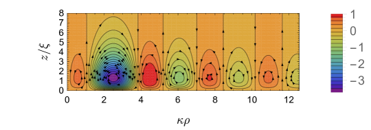
Figure 6: The colorplot of the magnetic field component $B^{(0)}_{\varphi}(\rho,z)/\tilde{B}$ and the corresponding current lines. Here we put $m=1$, $\alpha=1/\sqrt{2}$, $\beta=i/\sqrt{2}$, $\xi/\lambda=1/2$, $\xi/l_{E}=\sqrt{5.79}$, $\omega\tau=1$, $\kappa\lambda=2\cdot 10^{-3}$, $\theta=\pi/4$. The isolines of the $B^{(0)}_{\varphi}$ profiles coincide with the current lines $\mathbf{j}^{(0)}_{\text{sum}}$.

Let us finally briefly comment on the behavior of the small correction to the vector potential $\mathbf{a}^{(0)}$ and the phase gradient needed to get zero divergence of the total current. The equation for $\mathbf{a}^{(0)}$ reads:

$$\Delta\mathbf{a}^{(0)}-\frac{1}{\lambda^{2}}\mathbf{a}^{(0)}=\frac{\partial}{\partial z}\left(\frac{1}{\rho}\frac{\partial(\rho A^{(0)}_{0})}{\partial\rho}\right)\mathbf{e}_{z}-\nabla\chi^{(0)}-\frac{4\pi}{c}j^{(0)}_{\text{ph},z}\mathbf{e}_{z}$$ (58)

Here we impose the gauge $\operatorname{div}\mathbf{a}^{(0)}=0$ and $a_{z}=0$. Taking the divergence of the left- and right-hand sides of the equation (58) we get the Laplace equation by $\chi^{(0)}$:

$$\Delta\chi^{(0)}=-\frac{4\pi}{c}\frac{\partial j^{(0)}_{\text{ph},z}}{\partial z}+\frac{\partial^{2}}{\partial z^{2}}\left(\frac{1}{\rho}\frac{\partial(\rho A^{(0)}_{0})}{\partial\rho}\right)$$ (59)

The main term of the phase $\chi^{(0)}$ can be found integrating the above equation over $z$ twice (the constant of the integration $\chi^{(0)}(\infty)=0$):

$$\chi^{(0)}(\rho,z)=-\frac{4\pi}{c}\operatorname{Re}\Bigg{[}\int_{+\infty}^{z}f_{\text{ph}}(z^{\prime})dz^{\prime}\cdot j^{(c,0)}_{\text{ph},z}(\rho,0)+\\ +f_{\text{M}}(z)\lambda^{2}\frac{\partial(\rho j^{(c,0)}_{\text{ph},\rho}(\rho,0))}{\rho\partial\rho}\Bigg{]}$$ (60)

As noted above all these corrections are generally important to guarantee the absence of the current sources but do not provide essential contributions to the light induced magnetic fields.

V Interaction of a Bessel beam of twisted light with a superconducting thin film

Both linear and nonlinear electrodynamics considered above should be strongly affected by the sample geometry and, in particular, by its thickness. As soon as the thickness becomes comparable with the characteristic length scales one can expect the modification of current spatial distributions and resulting magnetic fields. Thus, keeping in mind possible experimental setup it is reasonable to generalize the above results for the case of a thin superconducting film of the thickness $d$ less than the London penetration depth. Similarly to the above analysis we need first to describe the generation of photocurrents by the incident plain wave. The expressions for the reflection coefficient similar to Eqs.(13), (14) for P- and S-polarizations take the form (see [41]):

$$r_{\parallel} =\frac{1}{1-\frac{2i\omega\lambda^{2}_{\text{eff}}}{c\cos{\theta}d}},$$ (61)

$$r_{\perp} =\frac{1}{1-\frac{2i\cos{\theta}\omega\lambda^{2}_{\text{eff}}}{cd}}.$$ (62)

Hereafter we assume that the film is not too thin, so that $\omega\lambda^{2}/cd\ll 1$ and, thus, the reflection coefficient appears to be close to unity and the magnetic field at the second boundary of the film is equal to zero. Taking $\omega\sim 10^{12}s^{-1}$ and $\lambda\sim 100\ nm$, we find that the above condition breaks down only when $d\lesssim 1\ nm$. Thus, we assume the film to be thicker than the atomic length scale.

A significant difference between the film and the bulk superconductor is the presence of a second boundary, which implies additional boundary conditions for the functions $H(z)$, $\tilde{\phi}(z)$ and $\Delta_{1}(z)$. Starting again from the case of the incident plane wave we find the resulting magnetic field distribution described by the expressions:

$$\mathbf{H}(z)=\mathbf{e}_{\text{H}}B_{0}e^{ik_{x}x}\times\begin{cases}\left(e^{ik_{z}z}+e^{-ik_{z}z}\right),z<0\ ,\\ 2\frac{\sinh{\frac{d-z}{\lambda_{\text{eff}}}}}{\sinh{\frac{d}{\lambda_{\text{eff}}}}},0<z<d\ ,\\ 0,z>d\ ,\end{cases}$$ (63)

where $\mathbf{e}_{\text{H}}=(\beta\cos\theta,\alpha,0)^{T}$. By analogy to the above calculation in the bulk we obtain both $\tilde{\phi}(z)$ (with two boundary conditions $\partial\tilde{\phi}/\partial z|_{z=0}=-E_{z}(z=0)=-\frac{i\omega\sin\theta}{2\pi\sigma_{n}}B_{0}$, $\partial\tilde{\phi}/\partial z|_{z=d}=-E_{z}(z=d)=0$) and $\Delta_{1}(z)$ (with two boundary conditions $\partial\Delta_{1}/\partial z=0$ at $z=0,d$):

$$\tilde{\phi}(z)=\alpha e^{ik_{x}x}\frac{2i\omega\sin\theta B_{0}}{4\pi\sigma_{n}q_{1}}\frac{\cosh{q_{1}(d-z)}}{\sinh{q_{1}d}}$$ (64)

$$\Delta_{1}(z)=\alpha e^{ik_{x}x}\frac{4e\tau\nu\Delta_{0}}{\hbar\xi^{2}}\frac{i\omega\sin\theta B_{0}}{4\pi\sigma_{n}(q_{2}^{2}-q_{1}^{2})}\times\\ \left(\frac{\cosh{q_{1}(d-z)}}{q_{1}\sinh{q_{1}d}}-\frac{\cosh{q_{2}(d-z)}}{q_{2}\sinh{q_{2}d}}\right)$$ (65)

Taking into account the $\Delta_{1}(z)$ dependence after integration over $z$ from 0 to $d$ we get the total current:

$$\mathbf{I}^{\text{film}}_{\text{ph},\parallel}=\frac{\lambda}{d}\frac{\nu}{\sqrt{2}\pi}\frac{\xi}{\tau}\frac{B_{0}^{2}\sin{\theta}}{H_{cm}}\frac{\omega\tau}{1+\omega^{2}\tau^{2}\eta^{2}}\times\\ \operatorname{Re}\left[\frac{i}{\sqrt{1-i\omega\tau\eta}}\frac{\sqrt{1+i\omega\tau\eta}}{2-i\omega\tau}\begin{pmatrix}|\alpha|^{2}\\ -\alpha\beta^{*}\cos{\theta}\\ -i|\alpha|^{2}\sin\theta\frac{\lambda\omega}{c\sqrt{1+i\omega\tau\eta}}\end{pmatrix}\right].$$ (66)

Further procedure of calculation of the photocurrent at zero frequency in the film for the case of the Bessel beam is straightforward:

$$\mathbf{j}^{(f,0)}_{\text{ph}}=\frac{\lambda}{d}\frac{\nu B_{0}^{2}\omega\sin\theta}{\sqrt{2}H_{cm}\xi\lambda^{2}l_{E}^{2}}\operatorname{Re}\Bigg{[}\frac{\lambda^{2}_{\text{eff}}}{q_{1}^{2}-q_{2}^{2}}\times\\ \left((q_{1}\tanh{q_{1}d})^{-1}-(q_{2}\tanh{q_{2}d})^{-1}\right)f^{(f)}_{\text{ph}}(z)\times\\ \begin{pmatrix}i_{1}(\rho)+i_{2}(\rho)\\ i_{3}(\rho)+i_{4}(\rho)\\ i_{5}(\rho)\end{pmatrix}\Bigg{]}$$ (67)

where $i_{1-5}(\rho)$ are given above (after the expression (32)), and

$$f^{(f)}_{\text{ph}}(z)=\frac{1}{(q_{1}\tanh{q_{1}d})^{-1}-(q_{2}\tanh{q_{2}d})^{-1}}\times\\ \Biggl{(}\frac{\cosh q_{1}(d-z)}{q_{1}\sinh q_{1}d}-\frac{\cosh q_{2}(d-z)}{q_{2}\sinh q_{2}d}\Biggr{)}\ .$$ (68)

The components of the Meissner screening current are described by the expressions:

$$\mathbf{j}^{(f,0)}_{\text{M}}(\rho,z)=-\frac{c}{4\pi\lambda^{2}}\mathbf{A}^{(f,0)}=\operatorname{Re}\Bigg{[}f^{(f)}_{\text{M}}(z)\mathbf{j}^{(c,f,0)}_{\text{ph}}(\rho,0)\Bigg{]}$$ (69)

with

$$f^{(f)}_{\text{M}}(z)=\frac{\lambda^{-2}}{(q_{1}\tanh{q_{1}d})^{-1}-(q_{2}\tanh{q_{2}d})^{-1}}\times\\ \Biggl{(}\frac{\cosh q_{1}(d-z)}{q_{1}Q_{1}\sinh q_{1}d}-\frac{\cosh q_{2}(d-z)}{q_{2}Q_{2}\sinh q_{2}d}-\\ \frac{\lambda^{2}}{d}\left(\frac{1}{Q_{1}}-\frac{1}{Q_{2}}\right)\Biggr{)}$$ (70)

and $Q_{1,2}=q_{1,2}^{2}-\lambda^{-2}$. The spatial profiles of the resulting photoinduced and Meissner currents in a thin film are shown in Fig. 7. Note that for a thin film with $d\ll\lambda$ the current density is almost homogeneous along the $z$-coordinate. Using the formula (57), we calculate also the magnetic field $\mathbf{B}=\operatorname{curl}\mathbf{A}$. $B^{(0)}_{\varphi}(\rho,z)$ distribution in the film and the current flow are shown in Fig. 8.

Note that the $B^{(0)}_{z}(\rho)$ profiles coincide with those for superconducting half-space up to a certain constant depending on the film thickness. The resulting vertical magnetic field in the film is of the order:

$$B^{(0)}_{z}\sim\nu\frac{\lambda^{2}}{d^{2}}\kappa^{2}\lambda\xi\frac{B_{0}^{2}}{H_{\text{cm}}}$$ (71)

which is larger than the half-space result by the factor $(\lambda/d)^{2}$ which can also be written as a ratio of the Pearl length $\lambda_{\text{Pearl}}=\lambda^{2}/d$ to the film thickness. The Pearl length is well known as a natural length scale determining the screening properties of thin superconducting films [46]. The first $\lambda/d$ multiplier in this product results from the increase of the superfluid velocity $\mathbf{v}_{s}$ at frequency $\omega$; the second $\lambda/d$ multiplier originates from the boundary conditions for the dc vector potential (following from the absence of the dc magnetic field outside the superconductor). The total factor $(\lambda/d)^{2}$ can strengthen the resulting photoinduced magnetic fields and, thus, facilitate the experimental observation of the above effects.

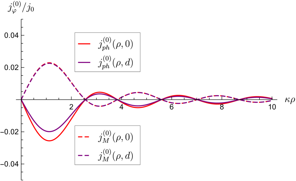
Figure 7: Typical photoinduced and Meissner current profiles for the film. Here we put $d=3\lambda/4$, $\lambda/\xi=2$, $l_{E}/\xi=1/\sqrt{5.79}$, $\omega\tau=1$, $\alpha=1/\sqrt{2},\beta=i/\sqrt{2},m=1,\theta=\pi/4$, $j_{0}=\nu B_{0}^{2}\omega\sin{\theta}/\sqrt{2}H_{\text{cm}}$.

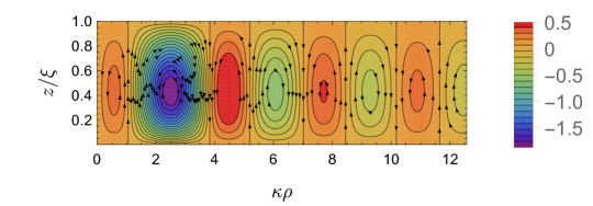
Figure 8: The colorplot of the magnetic field component $B^{(0)}_{\varphi}(\rho,z)/\tilde{B}$ and the corresponding current lines. Here we put $m=1$, $\alpha=1/\sqrt{2}$, $\beta=i/\sqrt{2}$, $d/\lambda=1/2$, $\xi/\lambda=1/2$, $\xi/l_{E}=\sqrt{5.79}$, $\omega\tau=1$, $\kappa\lambda=2\cdot 10^{-3}$, $\theta=\pi/4$. The isolines of the $B^{(0)}_{\varphi}$ profiles coincide with the current lines $\mathbf{j}^{(f,0)}_{\text{sum}}$.

VI Conclusion

To sum up, we have developed a phenomenological theory describing the interaction of structured electromagnetic radiation, specifically Bessel beams of twisted light, with superconducting systems and demonstrated that such beams can induce dissipationless dc photocurrents and associated magnetic fields that strongly depend on both the helicity and orbital angular momentum of light.

Our analysis revealed two mechanisms of the photoinduced magnetic response: (i) the transfer of the orbital momentum of the electromagnetic wave to the Cooper pairs; (ii) the inverse Faraday effect for the superconducting condensate caused by the helicity of the beam. The first contribution to the photocurrent is an odd function of the angular momentum quantum number $m$, while the second one is even in $m$. Both terms arise from the second order nonlinear response of the Cooper pairs resulting from the generation of the nonequilibrium charge imbalance potential which in turn affects the superfluid density due to a small particle-hole asymmetry.

We also provided detailed estimates of screening Meissner currents and derived explicit spatial profiles of induced magnetic fields, offering practical guidance for experimental detection using various magnetometry techniques. The presented results lay the groundwork for the experimental exploration of light-induced persistent currents in superconductors using structured light.

Appendix A Derivation of basic equations of perturbation theory in TDGL model

The aim of this section is to derive the equations for $\tilde{\phi}(\mathbf{r})$ and $\Delta_{1}(\mathbf{r})$ starting from basic TDGL equation (72):

$$-\Gamma\left(\hbar\frac{\partial}{\partial t}-2ie\phi\right)\Delta=\\ -aT_{c}\epsilon\Delta+b|\Delta|^{2}\Delta+aT_{c}\xi_{0}^{2}\left(-i\mathbf{\nabla}+\frac{2\pi}{\Phi_{0}}\mathbf{A}\right)^{2}\Delta.$$ (72)

Let us introduce a new variable $\tilde{\phi}=\phi-\frac{\hbar}{2e}\partial\chi/\partial t$. Taking the real part of Eq. (72) we get:

$$-\tau\frac{\partial\Delta_{1}}{\partial t}+\frac{2e}{\hbar}\tau\nu\Delta_{0}\tilde{\phi}=2\Delta_{1}-\xi^{2}\nabla^{2}\Delta_{1}.$$ (73)

After replacing $\partial/\partial t\rightarrow-i\omega$ we get:

$$-\nabla^{2}\Delta_{1}+q_{1}^{2}\Delta_{1}=\frac{2e\tau\nu\Delta_{0}}{\hbar\xi^{2}}\tilde{\phi},$$ (74)

where $q_{1}^{2}\equiv\frac{2-i\omega\tau}{\xi^{2}}$.

Multiplying the imaginary part of the Ginzburg-Landau equation (72) by the factor $4e\Delta^{*}/\hbar$ we find:

$$\operatorname{div}\mathbf{j}_{s}=\Delta_{0}^{2}\frac{4aT_{c}\xi_{0}^{2}\Delta_{0}^{2}e}{\hbar}\left(\Delta\chi-\frac{2\pi}{\Phi_{0}}\operatorname{div}\mathbf{A}\right)=\\ \frac{\pi a\Delta_{0}^{2}e^{2}}{\hbar}\tilde{\phi}.$$ (75)

The continuity equation reads:

$$\operatorname{div}\mathbf{j}_{s}=-\operatorname{div}\mathbf{j}_{n}=\sigma_{n}\operatorname{div}\left(\mathbf{\nabla}\phi+\frac{1}{c}\partial\mathbf{A}/\partial t\right).$$ (76)

Adding and subtracting $\pm\frac{\hbar}{2e}\nabla(\partial\chi/\partial t)$ in (76) and taking into account (75) and (76) together, we obtain:

$$\Delta\tilde{\phi}-\frac{\pi\hbar}{8T_{c}\xi_{0}^{2}}\partial\tilde{\phi}/\partial t=\frac{\pi a\Delta_{0}^{2}e^{2}}{\hbar\sigma_{n}}\tilde{\phi}.$$ (77)

Substituting $\partial/\partial t\rightarrow-i\omega$ we can write the final equation for the charge imbalance potential:

$$\Delta\tilde{\phi}=q_{2}^{2}\tilde{\phi},$$ (78)

where $q_{2}^{2}\equiv\frac{1}{l_{E}^{2}}-\frac{i\omega\tau}{\xi^{2}}=\frac{\lambda^{2}}{l_{E}^{2}\lambda_{\text{eff}}^{2}}$.

Appendix B Basic equations for electric and magnetic fields

Maxwell’s equations for the electromagnetic field inside the superconductor read:

$$\operatorname{curl}\mathbf{H}_{i}=\frac{4\pi\sigma_{n}}{c}\mathbf{E}_{i}+\frac{4\pi}{c}\mathbf{j}_{s}+\frac{1}{c}\frac{\partial\mathbf{D}_{i}}{\partial t}$$ (79)

$$\operatorname{curl}\mathbf{E}_{i}=-\frac{1}{c}\frac{\partial\mathbf{H}_{i}}{\partial t}$$ (80)

where $\mathbf{D}_{i}=\varepsilon\mathbf{E}_{i}$.

Using the London theory and exploiting the relation $\frac{\partial}{\partial t}\left(A-\frac{\Phi_{0}}{2\pi}\nabla\chi\right)\rightarrow-\frac{ic}{\omega}\left(\mathbf{E}+\nabla\tilde{\phi}\right)$ we find the expression for the current density written through the complex amplitudes:

$$\mathbf{j}_{s}=-\frac{c}{4\pi\lambda^{2}}\left(\mathbf{A}-\frac{\Phi_{0}}{2\pi}\nabla\chi\right)=i\frac{c^{2}}{4\pi\omega\lambda^{2}}\left(\mathbf{E}_{i}+\nabla\tilde{\phi}\right)\ .$$ (81)

After the Fourier transform in time variable we obtain the equation for the magnetic field:

$$\Delta\mathbf{H}_{i}=\left(\frac{1}{\lambda^{2}}-\frac{4\pi i\sigma_{n}\omega}{c^{2}}-\frac{\omega^{2}}{c^{2}}\varepsilon\right)\mathbf{H}_{i}$$ (82)

Neglecting the last term in parentheses and introducing the effective penetration depth

$$\frac{1}{\lambda_{\text{eff}}^{2}}=\frac{1}{\lambda^{2}}-\frac{4\pi i\sigma_{n}\omega}{c^{2}}=\frac{1}{\lambda^{2}}\left(1-i\omega\tau\frac{l_{E}^{2}}{\xi^{2}}\right),$$ (83)

we get the equations used in the main text:

$$\Delta\mathbf{H}_{i}=\frac{1}{\lambda_{\text{eff}}^{2}}\mathbf{H}_{i}\ ,$$ (84)

$$\operatorname{curl}\mathbf{H}=\frac{ic}{\omega}\left(\frac{1}{\lambda_{\text{eff}}^{2}}\mathbf{E}+\frac{1}{\lambda^{2}}\nabla\tilde{\phi}\right)\ .$$ (85)

Appendix C Field of twisted light in vacuum

In this section, we calculate the magnetic field of the incident twisted light in vacuum. The incident wave has two polarizations, so we introduce the polarization unit vector corresponding to the magnetic field direction:

$$\mathbf{e}_{\text{H}}=\alpha\mathbf{e}_{\text{H}}^{\parallel}+\beta\mathbf{e}_{\text{H}}^{\perp},$$ (86)

where $|\alpha|^{2}+|\beta|^{2}=1$, and $\sin\theta=\frac{\kappa}{k}$.

$$\mathbf{k}/k=(\sin\theta\cos\varphi_{k},\sin\theta\sin\varphi_{k},\cos\theta)^{T},$$ (87)

where $k^{2}=k_{\parallel}^{2}+k_{z}^{2}$, $\varphi_{k}\in[0,2\pi)$. Unit vectors for P-and S-polarizations can be written as follows:

$$\begin{cases}\mathbf{e}_{\text{H}}^{\parallel}=(-\sin\varphi_{k},\cos\varphi_{k},0)^{T},\\ \mathbf{e}_{\text{H}}^{\perp}=(\cos\theta\cos\varphi_{k},\cos\theta\sin\varphi_{k},-\sin\theta)^{T}.\end{cases}$$ (88)

Therefore, the complex amplitudes of the magnetic field of the incident wave $\mathbf{H}^{(e)}$ take the form:

$$\mathbf{H}^{(e)}=B_{0}e^{ik_{z}z}\int\frac{d^{2}\vec{k}_{\parallel}}{(2\pi)^{2}}e^{i\vec{k}_{\parallel}\vec{\rho}}a_{\kappa m}(k_{\parallel})\mathbf{e}_{\text{H}}.$$ (89)

where

$$a_{\kappa m}(k_{\parallel})=\frac{2\pi}{\kappa}i^{-m}\delta(\kappa-k_{\parallel})e^{im\varphi_{k}}.$$ (90)

In Cartesian coordinates the expression for the magnetic field can be rewritten as follows:

$$\mathbf{H}^{(e)}=\begin{pmatrix}H_{x}^{(e)}\\ H_{y}^{(e)}\\ H_{z}^{(e)}\end{pmatrix}=\frac{B_{0}}{2\pi}i^{-m}e^{ik_{z}z}\int d\varphi_{k}e^{i\mathbf{k}_{\parallel}\vec{\rho}}e^{im\varphi_{k}}\begin{pmatrix}-\alpha\sin\varphi_{k}+\beta\cos\theta\cos\varphi_{k}\\ \alpha\cos\varphi_{k}+\beta\cos\theta\sin\varphi_{k}\\ -\beta\sin\theta\end{pmatrix}=\\ =\frac{B_{0}}{2}e^{ik_{z}z+im\varphi}\begin{pmatrix}-e^{i\varphi}J_{m+1}(\kappa\rho)o_{-}-e^{-i\varphi}J_{m-1}(\kappa\rho)o_{+}\\ ie^{i\varphi}J_{m+1}(\kappa\rho)o_{-}-ie^{-i\varphi}J_{m-1}(\kappa\rho)o_{+}\\ -2\beta\sin\theta J_{m}(\kappa\rho)\end{pmatrix},$$ (91)

where $o_{\pm}=\alpha\pm i\beta\cos\theta$. It may be also useful to transform the above expression into the column vector written in cylindrical coordinate system ($\rho,\varphi,z$):

$$\mathbf{H}^{(e)}=\begin{pmatrix}H_{\rho}^{(e)}\\ H_{\varphi}^{(e)}\\ H_{z}^{(e)}\end{pmatrix}=\frac{B_{0}}{2}e^{ik_{z}z+im\varphi}\begin{pmatrix}-J_{m+1}(\kappa\rho)o_{-}-J_{m-1}(\kappa\rho)o_{+}\\ iJ_{m+1}(\kappa\rho)o_{-}-iJ_{m-1}(\kappa\rho)o_{+}\\ -2\beta\sin\theta J_{m}(\kappa\rho)\end{pmatrix}.$$ (92)

References

- [1] V. D. Plastovets, I. D. Tokman, B. Lounis, A. S. Mel’nikov, and A. I. Buzdin, All‑optical generation of Abrikosov vortices by the inverse Faraday effect, Phys. Rev. B 106, 174504 (2022).
- [2] M. D. Croitoru, S. V. Mironov, B. Lounis, and A. I. Buzdin, Toward the light-operated superconducting devices: Circularly polarized radiation manipulates the current-carrying states in superconducting rings, Adv. Quantum Technol. 5, 2200054 (2022).
- [3] L. P. Pitaevskii, Electric forces in a transparent dispersive medium, ZhETF 39, 1450 (1960) [Sov. Phys. JETP 12, 1008 (1961)].
- [4] S.V. Mironov, A.S. Mel’nikov, I.D. Tokman, V. Vadimov, B. Lounis, and A.I. Buzdin, Inverse Faraday effect for superconducting Condensates, Phys. Rev. Lett. 126, 137002, (2021).
- [5] M. Dzero, Inverse Faraday effect in superconductors with potential impurities, Phys. Rev. B 110, 054506 (2024).
- [6] L. Allen, M. W. Beijersbergen, R. J. C. Spreeuw, and J. P. Woerdman, Orbital angular momentum of light and the transformation of Laguerre-Gaussian laser modes, Phys. Rev. A 45, 8185, (1992).
- [7] A. Forbes, M. de Oliveira, and M. R. Dennis, Structured light, Nat. Photonics 15, 253–262 (2021).
- [8] L. Allen, M. J. Padgett, and M. Babiker, The orbital angular momentum of light, in Progress in Optics, edited by E. Wolf (Elsevier, Amsterdam, 1999), Vol. 39, pp. 291–372.
- [9] G. Molina-Terriza, J. P. Torres, and L. Torner, Twisted photons, Nat. Phys. 3, 305 (2007).
- [10] B. A. Knyazev and V. G. Serbo, Beams of photons with nonzero projections of orbital angular momenta: New results, Usp. Fiz. Nauk 188, 508 (2018) [Phys.-Usp. 61, 449 (2018)].
- [11] Z. Ji, W. Liu, S. Krylyuk, X. Fan, Z. Zhang, A. Pan, L. Feng, A. Davydov, and R. Agarwal, Photocurrent detection of the orbital angular momentum of light, Science 368, 763 (2020).
- [12] S. Sederberg, F. Kong, F. Hufnagel, C. Zhang, E. Karimi, and P. B. Corkum, Vectorized optoelectronic control and metrology in a semiconductor, Nat. Photonics 14, 680 (2020).
- [13] D. L. Andrews, Structured Light and Its Applications: An Introduction to Phase-Structured Beams and Nanoscale Optical Forces (Academic Press, Amsterdam, 2008).
- [14] V. I. Karpman and A. G. Shagalov, The ponderomotive force of a high-frequency electromagnetic field in a cold magnetized plasma, J. Plasma Phys. 27, 215 (1982).
- [15] R. Hertel, Theory of the inverse Faraday effect in metals, J. Magn. Magn. Mater. 303, L1 (2006).
- [16] A. V. Gaponov and M. A. Miller, Zh. Éksp. Teor. Fiz. 34, 242 (1958) [Sov. Phys. JETP 7, 168 (1958)].
- [17] V. I. Perel and Ya. M. Pinsky, Optical orientation of electrons in semiconductors, Sov. Phys. Solid State 15, 996 (1973).
- [18] H. M. Barlow, The Hall effect and its application to microwave power measurement, Proc. IRE 46, 1411 (1958).
- [19] J. H. Strait, G. Holland, W. Zhu, C. Zhang, B. R. Ilic, A. Agrawal, D. Pacifici, and H. J. Lezec, Confined plasmons in graphene nanoribbons, Phys. Rev. Lett. 123, 053903 (2019).
- [20] M. M. Glazov and S. D. Ganichev, High-frequency electric-field-induced nonlinear effects in graphene, Phys. Rep. 535, 101 (2013).
- [21] È. Normantas and G. E. Pikus, Drag effect at light reflection from the surface, Fiz. Tverd. Tela 27, 3017 (1985) [Sov. Phys. Solid State 27, 1762 (1985)].
- [22] M. V. Durnev and S. A. Tarasenko, Rectification of AC electric current at the edge of a two-dimensional electron gas, Phys. Status Solidi B 258, 2000291 (2021).
- [23] V. L. Gurevich and R. Laiho, Photomagnetism of metals: Microscopic theory of the photoinduced surface current, Phys. Rev. B 48, 8307 (1993).
- [24] V. L. Gurevich and A. Thellung, Photomagnetism of metals: Microscopic theory of photoinduced bulk current, Phys. Rev. B 49, 10081 (1994).
- [25] E. L. Ivchenko, Spin-dependent phenomena in semiconductors under high-frequency and photoexcitation, Phys. Status Solidi B 249, 2538 (2012).
- [26] A. A. Gunyaga, M. V. Durnev, and S. A. Tarasenko, Photocurrents induced by structured light, Phys. Rev. B 108, 115402 (2023).
- [27] A. A. Gunyaga, M. V. Durnev, and S. A. Tarasenko, Second harmonic generation due to the spatial structure of a radiation beam, Phys. Rev. Lett. 134, 156901 (2025).
- [28] M. V. Boev, Photon drag of superconducting fluctuations in two-dimensional systems, Phys. Rev. B 101, 104512 (2020).
- [29] A. V. Parafilo, M. V. Boev, V. M. Kovalev, and I. G. Savenko, Photogalvanic transport in fluctuating Ising superconductors, Phys. Rev. B 106, 144502 (2022).
- [30] M. V. Boev and V. M. Kovalev, Contribution of fluctuations of the order parameter to the second harmonic generation in two-dimensional monomolecular superconductors, Pis’ma Zh. Éksp. Teor. Fiz. 116, 173 (2022) [JETP Lett. 116, 173 (2022)].
- [31] V. Plastovets and A. I. Buzdin, Fluctuation-mediated inverse Faraday effect in superconducting rings, Phys. Lett. A 481, 129001 (2023).
- [32] S. V. Mironov, A. S. Mel’nikov, and A. I. Buzdin, ac Hall effect and photon drag of superconducting condensates, Phys. Rev. Lett. 132, 096001 (2024).
- [33] A. G. Aronov and A. B. Rapoport, Hall effect in superconductors above , Mod. Phys. Lett. B 6, 1083 (1992).
- [34] N. B. Kopnin, Theory of Nonequilibrium Superconductivity (Oxford University Press, Oxford, 2001).
- [35] T.-T. Yeh, H. Yerzhakov, L. Bishop-Van Horn, S. Raghu, and A. Balatsky, Structured light and induced vorticity in superconductors I: Linearly polarized light, arXiv:2407.15834 (2024).
- [36] T.-T. Yeh, H. Yerzhakov, L. Bishop-Van Horn, S. Raghu, and A. Balatsky, Structured light and induced vorticity in superconductors II: Quantum print with Laguerre–Gaussian beam, arXiv:2412.00935 (2024).
- [37] A. T. Dorsey, Vortex motion and the Hall effect in type-II superconductors: A time-dependent Ginzburg–Landau theory approach, Phys. Rev. B 46, 8376 (1992).
- [38] A. I. Larkin and A. A. Varlamov, in Physics of Conventional and Nonconventional Superconductors, edited by K.-H. Bennemann and J. B. Ketterson (Springer-Verlag, Berlin, 2002).
- [39] S. N. Artemenko and A. F. Volkov, Electric fields and collective oscillations in superconductors, Usp. Fiz. Nauk 128, 3 (1979) [Sov. Phys. Usp. 22, 295 (1979)].
- [40] B. I. Ivlev and N. B. Kopnin, Theory of current states in narrow superconducting channels, Usp. Fiz. Nauk 142, 435 (1984) [Sov. Phys. Usp. 27, 206 (1984)].
- [41] L. D. Landau and E. M. Lifshitz, Electrodynamics of Continuous Media, 2nd ed., Course of Theoretical Physics Vol. 8 (Pergamon, Oxford, 1984).
- [42] Y. Anahory, J. Reiner, L. Embon, D. Halbertal, A. Yakovenko, Y. Myasoedov, M. L. Rappaport, M. E. Huber, and E. Zeldov, Three-Junction SQUID-on-Tip with Tunable In-Plane and Out-of-Plane Magnetic Field Sensitivity, Nano Lett. 14, 6481 (2014).
- [43] C. W. Hicks et al., Noise characteristics of 100 nm scale GaAs/AlxGa1-xAs scanning Hall probes, Appl. Phys. Lett. 90, 133512 (2007).
- [44] R. A. Hovhannisyan, S. Yu. Grebenchuk, S. A. Larionov, A. G. Shishkin, A. K. Grebenko, N. E. Kupchinskaya, E. A. Dobrovolskaya, O. V. Skryabina, A. Yu. Aladyshkin, V. V. Dremov, I. A. Golovchanskiy, A. V. Samokhvalov, A. S. Mel’nikov, D. Roditchev, and V. S. Stolyarov, Scanning vortex microscopy reveals thickness-dependent pinning nano-network in superconducting niobium films, Commun. Mater. 6, 42 (2025).
- [45] Magneto-Optical Imaging, NATO Sci. Ser. II, Vol. 142, edited by T. H. Johansen and D. V. Shantsev (Kluwer Academic, Dordrecht, 2004).
- [46] J. Pearl, Current distribution in superconducting films carrying quantized fluxoids, Appl. Phys. Lett. 5, 65–66 (1964).