Why Do Stars Turn Red? II. Solutions of Steady-State Stellar Structure

Abstract

To investigate the physical origin of red giants (RGs) and red supergiants (RSGs), we construct steady-state models of stellar envelopes by explicitly solving the stellar structure equations, with boundary conditions set at the stellar surface and the hydrogen burning shell. For comparison, we consider both polytropic and realistic models. Polytropic models adopt a polytropic equation of state (EOS) and neglect energy transport, while realistic models incorporate radiative and convective energy transport, along with tabulated EOS and opacities. Our steady-state solutions reproduce three key features relevant to the evolution toward the RG/RSG phase. First, the refined mirror principle of Ou & Chen (2024) is reproduced: the stellar radius varies inversely with the radius of the envelope’s inner boundary, defined by the burning shell’s surface. This feature arises purely from hydrostatic equilibrium, as it appears in both polytropic and realistic models. Second, realistic models reveal an upper limit to envelope expansion, corresponding to an effective temperature of $\sim 4,000\,{\rm K}$, which is characteristic of RG/RSG stars and consistent with the classical Hayashi limit. Approaching this limit, the envelope undergoes a structural transition marked by a significant change in the density profile and the formation of an extended convective zone. The location of this limit is governed by the sharp drop in H^- opacity as the envelope cools below $\sim 10,000\,{\rm K}$. Finally, our solutions show that even a small shift in the envelope’s inner boundary can induce substantial envelope expansion throughout the yellow regime, naturally explaining the bifurcation of giants and supergiants into red and blue branches.

1 Introduction

The physical origin of red giants (RGs) and red supergiants (RSGs) remains one of the fundamental questions in stellar astrophysics. In Paper I of this series (Ou & Chen, 2024), we unveiled the mechanisms that drive stars to evolve into the RG/RSG using models with the stellar evolution code Modules for Experiments in Stellar Astrophysics (MESA; Paxton et al., 2011, 2013, 2015, 2018, 2019; Jermyn et al., 2023), version 10108. We showed that previous explanations based on energy absorption by the envelope are insufficient to account for the transition to the RG/RSG phase. Moreover, the conventional ”mirror principle,” which posits that the envelope expands in response to core contraction, does not always hold.

Instead, we identified a refined form of the mirror principle that persists throughout the envelope’s evolution: the envelope expands or contracts in the opposite direction to the motion of the boundary between the envelope and the hydrogen-burning shell. Specifically, there exists an inverse relationship between the stellar radius ($R_{*}$) and the inner radius of the envelope ($R_{\rm in}$, denoted as $R_{\rm shell}$ in Paper I). $R_{\rm in}$ is initially controlled by helium (He) core contraction and later by total nuclear energy generation from both the core and the hydrogen-burning shell, but consistently moves in the opposite direction to $R_{*}$.

By analyzing MESA models, we elucidated the physical origin of this refined mirror principle: as the shell-envelope boundary moves inward, its local gravitational acceleration increases. To maintain hydrostatic equilibrium, the pressure gradient must therefore steepen. Nonetheless, the pressure at the shell-envelope boundary is effectively fixed by nuclear burning conditions. The only way to increase the gradient under this constraint is to reduce the pressure, and hence the density, within the envelope. This reduced average density naturally leads to an expansion of the envelope.

However, it is difficult to validate this refined mirror principle using stellar evolution models alone, as they trace physical variables along specific evolutionary paths and do not allow exploration of all the configurations permitted by the stellar parameter space. To examine the relationship between $R_{*}$ and $R_{\rm in}$ more rigorously, we turn to solving steady-state stellar structures, which enable systematic examinations of the envelope structure for given stellar parameters.

In addition to the refined mirror principle, Paper I identified a notable structural transition that occurs as the star approaches the RG/RSG phase. Just before a star enters this phase, the outward expansion of the stellar surface temporarily stalls, whereas a large fraction of the interior mass is redistributed toward the outer envelope. This transition leads to increased opacity in most regions of the envelope, resulting in an extended convective zone that penetrates deeper toward the envelope’s base. In the present paper, we demonstrate that this structural transition naturally emerges from steady-state envelope solutions and investigate its physical origin in detail.

Furthermore, we aim to address a fundamental question: why do giant and supergiant stars converge to two distinct branches, red and blue? In our previous studies (Ou et al., 2023; Ou & Chen, 2025), we demonstrated a bimodal distribution of red and blue supergiants across stellar models with varying masses and metallicities, with very few models residing in the intermediate yellow regime. In the present study, by analyzing steady-state stellar envelope configurations, we gain new insights into the physical origin of this bimodal distribution.

This paper solves steady-state stellar envelope structures to investigate the refined mirror principle and uncover the physical significance of the RG/RSG phase. Section 2 defines the physical problem addressed in this work and describes the method we use to solve this problem. Section 3 begins with simplified polytropic envelope models. Section 4 presents realistic models that incorporate energy transport, using tabulated opacities and equations of state, together with convective mixing. Section 5 discusses the advantages, limitations, and implications of our approach. Finally, Section 6 summarizes our findings and concludes this study.

2 Methods

This study aims to solve a key physical question raised by the refined mirror principle introduced in Paper I: the relationship between the stellar radius and that of the shell-envelope boundary. As illustrated schematically in Figure 1, we approach this question by solving the envelope structure rather than modeling the evolution of the entire star. The envelope is defined as the stellar interior that does not contain active nuclear burning. Thus, the inner boundary in our calculation is not the center of the star but the shell-envelope boundary.

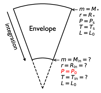
Figure 1: Schematic diagram illustrating the problem setup in this study. We integrate the stellar structure equations inward from the surface down to the inner boundary of the envelope, which is defined by a termination pressure $P_{0}$.

Most importantly, as demonstrated by the MESA models in Paper I, the inner boundary of the envelope is not set by a fixed enclosed mass but rather by a fixed pressure that reflects the physical conditions necessary to ignite shell hydrogen (H) burning. In our setup, we impose a constant pressure $P=P_{0}$ as the termination condition for the inward integration. The outer boundary of the envelope is defined at the stellar surface, where the radius is $R_{*}$ and the enclosed mass is $M_{*}$. By integrating inward from the stellar surface, we aim to determine the radius and enclosed mass at the envelope’s inner boundary, denoted by $R_{\rm in}$ and $M_{\rm in}$, respectively. We note that $R_{\rm in}$ and $M_{\rm in}$ are not prescribed parameters, but are instead outputs of the integration.

To compute the envelope structure, we solve the standard stellar structure equations along the mass coordinate $m$. The first equation expresses mass conservation:

$$\frac{dr}{dm}=\frac{1}{4\pi r^{2}\rho},$$ (1)

where $r$ is the radius, and $\rho$ is the density. The second equation enforces hydrostatic equilibrium:

$$\frac{dP}{dm}=-\frac{Gm}{4\pi r^{4}},$$ (2)

where $P$ is the pressure, and $G$ is the gravitational constant. The third equation governs energy transport by computing temperature $T$:

$$\frac{dT}{dm}=-\frac{GmT}{4\pi r^{4}P}\nabla,$$ (3)

The value of temperature gradient $\nabla$ depends on the mode of energy transport, either radiative or convective. We do not solve the fourth differential equation that governs energy conservation:

$$\frac{dl}{dm}=\epsilon_{\rm nuc}+\epsilon_{\rm grav}-\epsilon_{\nu}.$$ (4)

Here, $l$ is the local luminosity, $\epsilon_{\rm{nuc}}$ is the nuclear energy generation rate, $\epsilon_{\nu}$ is the neutrino loss rate, and $\epsilon_{\rm{grav}}$ is the gravothermal term. Within the envelope, $\epsilon_{\rm nuc}$ is negligible due to the absence of nuclear burning, and $\epsilon_{\nu}$ is typically small compared to the radiative flux, allowing both terms to be ignored. The remaining term $\epsilon_{\rm grav}$ depends on structural changes such as expansion or contraction. Thus, this term contains an evolution effect that requires information from the preceding time step. By assuming a steady-state envelope, we simply set $\epsilon_{\rm grav}=0$. Therefore, the luminosity is taken as a constant parameter $L_{0}$ and is uniform throughout the envelope. This simplification eliminates any internal luminosity gradient, effectively removing time-dependent factors and allowing us to focus on the steady-state structure.

With constant luminosity in the envelope, we solve the steady-state stellar structure within the envelope using the direct-shooting method. For a given stellar radius $R_{*}$, we specify the surface boundary conditions at $r=R_{*}$, which include the surface temperature $T_{\rm s}$ and the surface pressure $P_{\rm s}$. Starting from these surface conditions, we solve the stellar structure equations by integrating physical quantities inward. The integration is terminated when the pressure reaches the target value, $P=P_{0}$, which corresponds to the condition of the shell-envelope interface. Here, we adopt the fiducial value of $P_{0}=1.0\times 10^{16}\,{\rm dyne}\,{\rm cm}^{-2}$, estimated from Figure 10 in Paper I.

2.1 Polytropic models

Before solving the full set of equations, we first consider a simplified polytropic model, in which the gas obeys a power-law equation of state (EOS) relating the pressure $P$ to the density $\rho$:

$$P=K\rho^{\gamma},$$ (5)

where $K$ is the polytropic constant and $\gamma$ is the polytropic exponent. In this polytropic model, the density depends solely on pressure and is independent of temperature. Therefore, the equation of hydrostatic equilibrium is decoupled from energy transport (e.g., Prialnik, 2009). This simplification allows us to solve only the two fundamental structure equations, Equations (1) and (2), without calculating the temperature.

To integrate these equations, we impose a surface boundary condition on the pressure:

$$P_{\rm s}=\frac{\tau_{\rm s}g}{\kappa_{\rm s}},$$ (6)

where we adopt a surface optical depth of $\tau_{\rm s}=2/3$. Since temperature is not included in this model, we cannot use opacity tables that depend on temperature, density, and metallicity (e.g., Iglesias & Rogers, 1996). Instead, we assume a constant opacity $\kappa_{\rm s}=0.34\,{\rm cm}^{2}\,{\rm g}^{-1}$, representative of electron scattering in fully ionized hydrogen. The surface gravity is given by $g=GM_{*}/R_{*}^{2}$, and hence the surface pressure scales as $P_{\rm s}\propto R_{*}^{-2}$.

2.2 Realistic models

To construct realistic models, we require detailed gas physics such as the EOS and opacity. These data are retrieved from MESA (version 10108), with linear interpolation applied over the tabulated grids.

For the EOS, we adopt the MESA “eosPT” tables (Paxton et al., 2011), which take pressure and temperature as input parameters. Specifically, we average two tables, both with metallicity $Z=0.02$, but with hydrogen mass fractions of $X=0.6$ and $X=0.8$. The resulting table is treated as representative of $X=0.7$ and $Z=0.02$. From this table, we extract several thermodynamic quantities as functions of $P$ and $T$: the density $\rho(P,T)$, adiabatic temperature gradient $\nabla_{\rm ad}(P,T)$, specific heat at constant pressure $C_{P}(P,T)$, $\chi_{T}(P,T)\equiv(\partial\ln P/\partial\ln T)_{\rho}$, and $\chi_{\rho}(P,T)\equiv(\partial\ln P/\partial\ln\rho)_{T}$.

The opacity $\kappa(\rho,T)$ is taken from the “OP_-gs98” table in MESA, which combines the OPAL (Iglesias & Rogers, 1993, 1996) and OP (Seaton, 2005) tables. For simplicity, we do not use Type 2 opacities that consider the effect of carbon and oxygen enhancement.

We now define the two surface boundary conditions. The surface temperature ($T_{\rm s}$) is taken to be the effective temperature ($T_{\rm eff}$) of the star:

$$T_{\rm s}=T_{\rm eff}=\bigg{(}\frac{L_{0}}{4\pi R_{*}^{2}\sigma}\bigg{)}^{1/4}.$$ (7)

where $L_{0}$ is the stellar luminosity and $\sigma$ is the Stefan-Boltzmann constant. $L_{0}$ is treated as a constant throughout the envelope and is specified as an input parameter in our calculations. The surface pressure is set using the “simple photosphere” prescription in MESA (Paxton et al., 2011):

$$P_{\rm s}=\frac{\tau_{\rm s}g}{\kappa_{\rm s}}\bigg{[}1+1.6\times 10^{-4}\kappa_{\rm s}\bigg{(}\frac{L_{0}/L_{\odot}}{M_{*}/M_{\odot}}\bigg{)}\bigg{]},$$ (8)

where we adopt $\tau_{\rm s}=2/3$ and express the surface gravity as $g=GM_{*}/R_{*}^{2}$. Since $\kappa_{\rm s}$ is a function of $\rho$ and $T$, and $\rho$ is itself a function of $P$ via the EOS, the right-hand side of Equation (8) implicitly depends on $P_{\rm s}$. Therefore, $P_{\rm s}$ cannot be expressed explicitly, and we solve Equation (8) numerically to determine $P_{\rm s}$ for a given $R_{*}$.

Unlike in the polytropic models, the realistic models solve for the temperature profile via the energy transport equation. Whether energy is transported by radiation or convection is determined by comparing the radiative temperature gradient $\nabla_{\rm rad}$ with the adiabatic gradient $\nabla_{\rm ad}$. The radiative gradient is computed by

$$\nabla_{\rm rad}=\frac{3}{16\pi acG}\frac{\kappa lP}{mT^{4}},$$ (9)

where $a$ is the radiation density constant and $c$ is the speed of light. The adiabatic gradient $\nabla_{\rm ad}(P,T)$ is obtained from the EOS table. If the Schwarzschild criterion for convective stability ($\nabla_{\rm rad}<\nabla_{\rm ad}$) is satisfied, the energy is transported predominately by radiation, and we set the actual temperature gradient $\nabla$ equal to $\nabla_{\rm rad}$.

If instead $\nabla_{\rm rad}\geq\nabla_{\rm ad}$, then the transport of convective energy must be taken into account using mixing-length theory (MLT). Following the formulation of Kippenhahn et al. (2013), the MLT framework solves for five quantities: the radiative flux $F_{\rm rad}$, the convective flux $F_{\rm con}$, the element temperature gradient $\nabla_{\rm e}$, the actual temperature gradient $\nabla$, and the convective velocity $v$. The total flux is the sum of the radiative and convective components:

$$F_{\rm rad}+F_{\rm con}=\frac{4acG}{3}\frac{T^{4}m}{\kappa Pr^{2}}\nabla_{\rm rad}.$$ (10)

The radiative flux is given by

$$F_{\rm rad}=\frac{4acG}{3}\frac{T^{4}m}{\kappa Pr^{2}}\nabla.$$ (11)

The convective velocity is calculated using

$$v^{2}=g\delta(\nabla-\nabla_{\rm e})\frac{l^{2}_{\rm m}}{8H_{P}},$$ (12)

where $\delta\equiv-\left(\partial\ln\rho/\partial\ln T\right)_{P}=\chi_{T}/\chi_{\rho}$, and $H_{P}\equiv-dr/d\ln P$ is the pressure scale height. The mixing length $l_{\rm m}$ is taken as $l_{\rm m}=\alpha H_{P}$, with a mixing-length parameter $\alpha=1.5$ used in this work. The convective flux is then expressed as

$$F_{\rm con}=\rho C_{P}T\sqrt{g\delta}\frac{l^{2}_{\rm m}}{4\sqrt{2}}H_{P}^{-3/2}(\nabla-\nabla_{\rm e})^{3/2}.$$ (13)

Finally, the relationship between the four temperature gradients is given by

$$\frac{\nabla_{\rm e}-\nabla_{\rm ad}}{\nabla-\nabla_{\rm e}}=\frac{6acT^{3}}{\kappa\rho^{2}C_{P}l_{\rm m}v}.$$ (14)

Using this MLT framework, we can compute the actual temperature gradient $\nabla$ in Equation (3), accounting for the transport of radiative and convective energy.

However, directly solving the full set of five MLT equations can be a numerical challenge. To simplify the calculation, we adopt the approach described by Kippenhahn et al. (2013), which introduces two dimensionless quantities: $U\equiv(3acT^{3}/C_{P}\rho^{2}\kappa l^{2}_{\rm m})\sqrt{(8H_{P}/g\delta)}$ and $W\equiv\nabla_{\rm rad}-\nabla_{\rm ad}$. With these definitions, the actual temperature gradient $\nabla$ can be obtained by solving a single cubic equation:

$$(\xi-U)^{3}+\frac{8U}{9}(\xi^{2}-U^{2}-W)=0,$$ (15)

where $\xi$ is defined by this relation

$$\nabla=\xi^{2}+\nabla_{\rm ad}-U^{2}.$$ (16)

Once the root $\xi$ in Equation (15) is found, the actual temperature gradient $\nabla$ can be obtained. This value of $\nabla$ can then be substituted back into the energy transport equation in Equation (3) to solve the stellar structure.

3 Results from Polytropic Models

To explore the relationship between $R_{\rm in}$ and $R_{*}$ solely under the effect of hydrostatic equilibrium, we construct polytropic models for $25\,M_{\odot}$ stars. We assume a fixed $K=5.0\times 10^{15}$, such that the pressure and density scale as $P=(5.0\times 10^{15})\rho^{\gamma}$. Figure 2 presents the resulting values of $R_{\rm in}$ and $M_{\rm in}$ as functions of $R_{*}$ for various choices of $\gamma$. The value of $\gamma$ is adjusted to reproduce the typical values of $R_{\rm in}$ and $M_{\rm in}$ found in MESA stellar evolution models (as shown in Paper I) for $25\,M_{\odot}$ stars during the core He-burning phase: $R_{\rm in}\sim 1.0\,R_{\odot}$ and $M_{\rm in}\sim 10\,M_{\odot}$. The results show that when $\gamma\sim 1.3$ and $R_{*}\gtrsim 10\,R_{\odot}$, the above values $R_{\rm in}$ and $M_{\rm in}$ from the stellar evolution models can be reproduced. Remarkably, in these parameter regimes, the models consistently exhibit negative slopes between $R_{\rm in}$ and $R_{*}$, indicating that the mirror principle holds. Conversely, when the mirror principle is not satisfied, such as when $\gamma$ is far from $\sim 1.3$, or when $R_{*}\lesssim 10\,R_{\odot}$, the resulting values of $R_{\rm in}$ and $M_{\rm in}$ deviate substantially from those expected from realistic stellar evolution. It is worth noting that post-main-sequence stars of $25\,M_{\odot}$ typically have radii greater than $\sim 10\,R_{\odot}$, as shown in Paper I; therefore, they are in the parameter regime where the mirror principle is satisfied. To sum up, in these polytropic models, the mirror principle generally holds for envelope configurations that are physically reasonable for post-main-sequence stars.

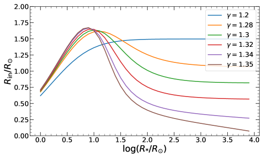
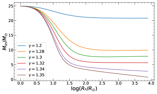
Figure 2: Radius ($R_{\rm in}$, top panel) and enclosed mass ($M_{\rm in}$, bottom panel) at the envelope’s inner boundary for polytropic models of $K=5.0\times 10^{15}$ but different $\gamma$.

These results demonstrate that hydrostatic equilibrium alone, without involving energy transport, can reproduce the mirror principle for post-main-sequence stars. To further investigate its physical origin, Figure 3 shows the pressure and density profiles for models with $\gamma=1.3$ but different values of $R_{*}$, plotted in both the mass and the radius coordinates. For clarity, we briefly recall the integration setup described in Section 2. Each model is integrated inward from $m=25\,M_{\odot}$ and $r=R_{*}$ until the pressure reaches the termination value $P=P_{0}$, at which point the values of $M_{\rm in}$ and $R_{\rm in}$ are determined.

We first examine the $\log P$ versus $m$ profiles. At the stellar surface, all models share the same enclosed mass $m=25\,M_{\odot}$, so the pressure gradient follows $dP/dm\propto r^{-4}$. Thus, a larger $R_{*}$ results in a flatter $dP/dm$ in the outer envelope. After integrating inward to a given $P$, models with a larger $R_{*}$ and therefore flatter $dP/dm$ traverse a larger mass, leading to a smaller enclosed mass $m$. This smaller $m$ reduces the gravitational acceleration $g$, which in turn affects the $\log P$ versus $\log r$ profiles. At a given $P$, the density is fixed due to the polytropic relation. According to the hydrostatic equilibrium equation in radius coordinates, $dP/dr=-\rho g$, a fixed $\rho$ implies that $dP/dr$ is set directly by $g$. Therefore, at a given $P$, the models with larger $R_{*}$ exhibits flatter $dP/dr$ due to weaker $g$, as shown in the $\log P$ versus $\log r$ profiles.

The difference in $dP/dr$ within the envelope for models with different $R_{*}$ further determines the resulting $R_{\rm in}$. We compare the three models with $R_{*}\gtrsim 10\,R_{\odot}$ in Figure 3, corresponding to $\log(R_{*}/R_{\odot})=1.5$, 2.0, and 2.5. Since models with larger $R_{*}$ exhibit flatter $dP/dr$, their $\log P$ versus $\log r$ profiles intersect and reverse order near $\log(r/R_{\odot})\sim 1.0$. Beyond the intersection point, the shallower $dP/dr$ in models with larger $R_{*}$ requires integration toward smaller radii to reach the termination pressure $P=P_{0}$. As a result, models with larger $R_{*}$ end up with smaller $R_{\rm in}$, illustrating the mirror principle.

For models with $R_{*}\lesssim 10\,R_{\odot}$ (i.e., $\log(R_{*}/R_{\odot})\lesssim 1$), the trend of flatter $dP/dr$ for larger $R_{*}$ still holds. However, in this regime, the termination pressure $P=P_{0}$ is reached before the pressure profiles intersect. As a result, models with larger $R_{*}$ continue to produce larger $R_{\rm in}$, and no reversal occurs. The mirror principle therefore does not hold in this parameter range. Nevertheless, as previously noted, these models yield $M_{\rm in}$ values that are significantly higher than those expected in the post-main-sequence evolution.

The above discussion explains the mirror principle from the perspective of our integration scheme, which proceeds inward from the stellar surface. We now consider the same physical system from the opposite viewpoint, starting from the inner boundary, to understand how the envelope “responds” to the core. In this perspective, for models with $R_{*}\gtrsim 10\,R_{\odot}$, the pressure gradient $dP/dm$ near the inner boundary becomes steeper as $R_{\rm in}$ moves inward. For example, comparing models with $\log(R_{*}/R_{\odot})=1.5$ and 2.5, the latter exhibits a smaller $R_{\rm in}$ by about 30% and a reduced $M_{\rm in}$ by approximately 20%. Since the pressure gradient near the inner boundary scales as $|dP/dm|_{\rm in}\sim M_{\rm in}\,R_{\rm in}^{-4}$, the model with $\log(R_{*}/R_{\odot})=2.5$, which has the smaller $R_{\rm in}$ and $M_{\rm in}$, exhibits a much steeper gradient. This steep pressure gradient causes the pressure to drop rapidly outwards, which in turn leads to a steep decline in density. The resulting low-density envelope extends to a much larger radius, making the overall envelope more extended. This physical mechanism is consistent with the result from the MESA models shown in Paper I.

Thus, the “response” of the envelope to its inner boundary can be understood as follows: With a smaller $R_{\rm in}$, the stronger gravity at the shell-envelope interface requires a steeper outward pressure gradient to sustain hydrostatic equilibrium, which is achieved through envelope expansion that reduces the pressure and density in the outer layers. As long as $M_{\rm in}$ is not excessively large (i.e., the core does not dominate the total mass), the inverse relationship between $R_{\rm in}$ and $R_{*}$ is generally valid.

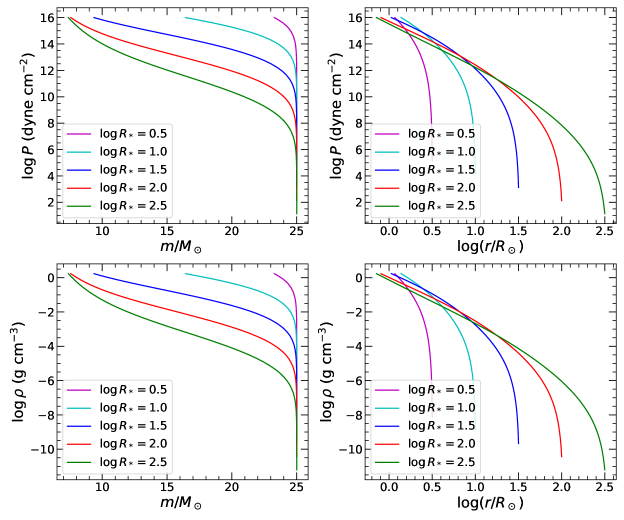
Figure 3: Pressure and density profiles for polytropic models with $\gamma=1.3$ and varying stellar radius $R_{*}$. Profiles are shown as functions of both mass and radius coordinates. Stellar radii $R_{*}$ are in units of $R_{\odot}$.

4 Results from Realistic models

After analyzing the polytropic models, we now construct realistic stellar envelope models that incorporate temperature calculations, EOS and opacity tables, and the MLT treatment for convection. As representative cases, we present models with initial masses of 5 and $25\,M_{\odot}$. For each model, we compute the structure of the steady-state envelope adopting a fixed internal luminosity $L_{0}$, which is assumed to be constant throughout the envelope. Based on the MESA models presented in Paper I, we set $L_{0}=(6$–$10)\times 10^{38}\,{\rm erg\,s}^{-1}$ for the $25\,M_{\odot}$ models, and $L_{0}=(4$–$12)\times 10^{36}\,{\rm erg\,s}^{-1}$ for the $5\,M_{\odot}$ models.

Figure 4 presents the results for the $25\,M_{\odot}$ models with different values of $L_{0}$, showing the relationships among $R_{\rm in}$, $M_{\rm in}$, $R_{*}$, and $T_{\rm eff}$. The general trend of $R_{\rm in}$ versus $R_{*}$ resembles that seen in polytropic models: the mirror principle appears to hold when $M_{\rm in}$ lies in the physically reasonable range ($\sim 10\,M_{\odot}$). However, a notable difference from the polytropic models emerges near $R_{*}\sim 1,000\,R_{\odot}$, the characteristic radius of RSGs. In this region, $R_{\rm in}$ initially increases slightly with $R_{*}$ before undergoing a sharp decline. As shown in the bottom panel of Figure 4, during this sharp drop, $T_{\rm eff}$ for all models converge at the surface temperatures of $\sim 4000\,{\rm K}$ (i.e., $\log(T_{\rm eff}/{\rm K})\sim 3.6$), consistent with the typical effective temperatures of RSGs. The $5\,M_{\odot}$ models, presented in Figure 5, exhibit a similar pattern. The mirror principle begins to apply when $R_{*}\gtrsim$ a few $R_{\odot}$, and an abrupt drop in $R_{\rm in}$ occurs at $R_{*}\sim 100\,R_{\odot}$ and $T_{\rm eff}\sim 4,000$–$4,500\,{\rm K}$, marking the RG phase for lower-mass stars.

Importantly, this sharp drop in $R_{\rm in}$ near the RG/RSG radii defines an upper limit to stellar expansion. Even as $R_{\rm in}$ contracts to small values, the envelope cannot expand beyond this threshold. Hence, the RG/RSG phase emerges as a limiting configuration for envelope expansion in steady-state solutions. Furthermore, in the RG / RSG solution, the curve $R_{\rm in}$ becomes nearly vertical in the $R_{\rm in}$–$R_{*}$ plane, indicating that variations in $R_{\rm in}$ have little impact on $R_{*}$. As a result, once a star enters this regime, the RG/RSG structure behaves as a stable state, remaining largely unaffected by any moderate change in $R_{\rm in}$.

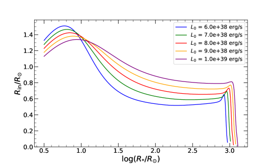
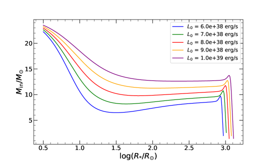
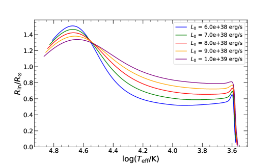
Figure 4: $R_{\rm in}$ versus $R_{*}$ (top panel), $M_{\rm in}$ versus $R_{*}$ (middle panel), and $R_{\rm in}$ versus $T_{\rm eff}$ (bottom panel) of $25\,M_{\odot}$ stars with different luminosities $L_{0}$.

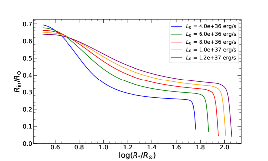
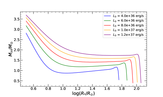
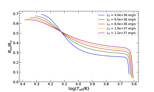
Figure 5: $R_{\rm in}$ versus $R_{*}$ (top panel), $M_{\rm in}$ versus $R_{*}$ (middle panel), and $R_{\rm in}$ versus $T_{\rm eff}$ (bottom panel) of $5\,M_{\odot}$ stars with different luminosities $L_{0}$.

4.1 Structural Transition Toward the Red Giant/Supergiant Phase

To understand the physical significance of the RG/RSG solution, Figure 6 presents the structural profiles of $25\,M_{\odot}$ stellar models at three stages as they expand toward the RSG regime, with radii of approximately $800\,R_{\odot}$, $1,000\,R_{\odot}$, and $1,050\,R_{\odot}$ (corresponding to $\log(R_{*}/R_{\odot})=2.9$, 3.0, and 3.02, respectively).

These profiles reveal pronounced structural changes during the final phase of expansion toward the RSG radii. At $R_{*}\sim 800\,R_{\odot}$, only a small portion of the stellar mass extends to large radii. At a mass coordinate of $m\sim 23\,M_{\odot}$, the radial position remains relatively compact at $r\sim 30\,R_{\odot}$. Only the outermost $\sim 2\,M_{\odot}$ of the envelope is distributed between $\sim 30\,R_{\odot}$ to $\sim 800\,R_{\odot}$. As $R_{*}$ increases, the mass distribution changes dramatically. At $R_{*}\sim 1,050\,R_{\odot}$, the position of $m\sim 12\,M_{\odot}$, which is only $\sim 2\,M_{\odot}$ above the inner boundary of the envelope, is already located at $r\sim 150\,R_{\odot}$. As the star expands from $800$ to $1,050\,R_{\odot}$, a significant portion of the envelope mass is redistributed outward, markedly altering the radius profile. This redistribution of mass is also evident in the density profiles. At $R_{*}\sim 800\,R_{\odot}$, most of the envelope remains relatively compact, with densities $\rho>10^{-4}\,{\rm g\,cm}^{-3}$, and only the outermost layers reach lower densities. In contrast, at $R_{*}\sim 1,050\,R_{\odot}$, the density drops sharply near the base of the envelope, from $\sim 1\,{\rm g\,cm}^{-3}$ at $m=10\,M_{\odot}$ to $<10^{-6}\,{\rm g\,cm}^{-3}$ at $m=11\,M_{\odot}$.

The temperature profiles also exhibit dramatic differences as $R_{*}$ increases. At $R_{*}\sim 800\,R_{\odot}$, the region near $m=23\,M_{\odot}$ remains hot, with temperatures near $10^{6}\,{\rm K}$. Only the outermost layers cool below $\sim 10^{6}\,{\rm K}$. By the time the star reaches $R_{*}\sim 1,050\,R_{\odot}$, nearly the entire envelope has cooled to $\lesssim 10^{6}\,{\rm K}$. This temperature drop has a profound effect on the opacity. In the temperature range $10^{4}$–$10^{7}\,{\rm K}$, the opacity generally follows the Kramers’ law, $\kappa\propto\rho T^{-3.5}$, and thus increases as the temperature decreases. As the envelope cools by 1.5–2 orders of magnitude between $R_{*}\sim 800$ and $1,050\,R_{\odot}$, the opacity increases significantly throughout most of the envelope mass.

This enhancement in opacity leads to a critical structural transition: the development of an extended convective envelope. The elevated opacity increases the radiative temperature gradient $\nabla_{\rm rad}$, well above the adiabatic gradient $\nabla_{\rm ad}$, thus triggering convection. As the star expands and deeper layers cool into the high-opacity regime, the convective zone penetrates into the base of the envelope. Eventually, nearly the entire envelope becomes convective. As shown in the bottom-left panel of Figure 6, at $R_{*}\sim 800\,R_{\odot}$, only a few localized convective zones are present, each confined to a small fraction of the envelope mass. By $R_{*}\sim 1,000\,R_{\odot}$, the surface convective zone has been extended to reach a mass coordinate of $m\sim 16.5\,M_{\odot}$. When the star reaches $R_{*}\sim 1,050\,R_{\odot}$, the convective region spans almost the entire envelope.

These processes of mass redistribution and the formation of an extended convective zone are highly consistent with the MESA stellar evolution models, as presented in Section 6 of Paper I. Our steady-state solutions now reproduce this structural transition, demonstrating that the RG/RSG configuration is not merely an outcome of stellar evolution but a physically required state for stars achieving such large radii. Specifically, for a $25\,M_{\odot}$ star, once the stellar radius exceeds $\gtrsim 1,000\,R_{\odot}$, the envelope necessarily adopts an RG/RSG structure with an extended convection zone.

This result highlights the physical significance of the phase transition. The nearly vertical drop in $R_{\rm in}$ with respect to $R_{*}$ in $R_{*}\sim 1,000\,R_{\odot}$ coincides with the completion of the phase transition to RG / RSG. This indicates that, beyond this point, the stellar radius cannot increase further. The structural profiles reveal that after the transition, the pressure and temperature gradients across the envelope become extremely shallow. If the radius were to increase further, these gradients would flatten even more, making it impossible for the integration to reach the termination pressure $P_{0}$ within the remaining stellar mass. Therefore, for a star with an envelope above an H-burning shell, no steady-state solution exists beyond this limiting radius.

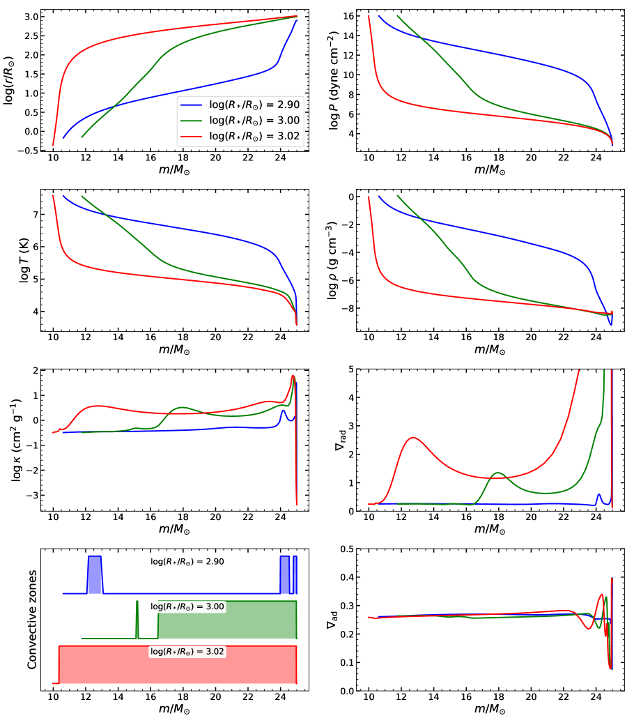
Figure 6: Profiles of radius ($r$), pressure ($P$), temperature ($T$), density ($\rho$), opacity ($\kappa$), radiative temperature gradient ($\nabla_{\rm rad}$), convective zones, and adiabatic temperature gradient ($\nabla_{\rm ad}$) for $25\,M_{\odot}$ stars with different stellar radii. The blue, green, and red curves correspond to stellar radii of $\log(R_{*}/R_{\odot})=2.90$, 3.00, and 3.02 ($R_{*}\sim 800$, 1,000, and 1,050$\,R_{\odot}$), respectively, illustrating steady-state envelope solutions that roughly represent several time points as the star approaches the RSG phase. In the bottom-left panel, the color blocks represent the location of convective zones for different $R_{*}$.

4.2 Physical Origin of the Red Giant/Supergiant Solution

To explore the physical origin of the RG/RSG solution, we conduct a series of controlled experiments by disabling individual physical treatments: convection, surface boundary condition from atmospheric models, and opacity interpolation from tables. All models assume a stellar mass of $25\,M_{\odot}$ and a fixed luminosity of $L_{0}=8.0\times 10^{38}\,{\rm erg\,s}^{-1}$. We consider the following model setups:

1. Standard model: Includes MLT for convection, interpolated opacity from tabulated data, and a simple atmospheric model to determine the surface pressure boundary condition.

2. No convection: Convection is disabled by turning off the MLT. The energy transport throughout the envelope is purely radiative, i.e. $\nabla=\nabla_{\rm rad}$ everywhere.

3. Constant surface pressure: The outer boundary condition is replaced by a fixed surface pressure. Three values are tested: $P_{\rm s}=1.0\times 10^{4}\,{\rm dyne\,cm}^{-2}$, $1.0\times 10^{3}\,{\rm dyne\,cm}^{-2}$, and $1.0\,{\rm dyne\,cm}^{-2}$.

4. Opacity floor: Imposes a minimum opacity using four values: $\kappa\geq 0.01$, $0.1$, $0.34$, and $1.0\,{\rm cm}^{2}\,{\rm g}^{-1}$.

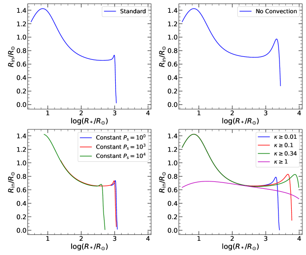
Figure 7: Relationship between $R_{\rm in}$ and $R_{*}$ for experiments modifying envelope properties on a $25\,M_{\odot}$ star. The upper-left panel shows results from the standard setup, while the upper-right panel presents the model without convection. The lower-left panel displays models with constant surface pressures of $10^{0}$, $10^{3}$, and $10^{4}\,{\rm dyne\,cm}^{-2}$. The lower-right panel shows models with a minimum opacity floor of $\kappa=0.01$, 0.1, 0.34, and $1.0\,{\rm cm}^{2}\,{\rm g}^{-1}$.

Figure 7 presents the $R_{\rm in}$–$R_{*}$ relationships for these models. We begin by comparing the standard model with the case in which convection is disabled. In the absence of convection, the $R_{\rm in}$–$R_{*}$ trend remains similar to the standard case for $R_{*}<1,000\,R_{\odot}$. However, an apparent difference emerges beyond this radius. In the convective model, $R_{\rm in}$ drops sharply once $R_{*}\gtrsim 1,000\,R_{\odot}$, indicating the transition to the RSG phase. In contrast, the non-convective model shows a continued increase in $R_{\rm in}$ up to $\sim 1,500\,R_{\odot}$, followed by a sudden drop in larger radii.

For models with constant surface pressure, the RSG transition changes depending on the value $P_{\rm s}$. A value of $P_{\rm s}=1.0\times 10^{3}\,\rm{dyne\,cm}^{-2}$ produces results similar to the standard model. Increasing $P_{\rm s}$ to $1.0\times 10^{4}\,\rm{dyne\,cm}^{-2}$ moves the RSG transition to a smaller radius ($R_{*}\sim 700\,R_{\odot}$). On the other hand, reducing the surface pressure to $P_{\rm s}=1.0\,{\rm dyne}\,{\rm cm}^{-2}$ produces a result very similar to the standard case, indicating that even a significantly reduced $P_{\rm s}$ has minimal effect on the RSG solution.

Opacity modifications produce the most dramatic changes in the $R_{\rm in}$–$R_{*}$ relation. For $\kappa\geq 0.01\,\rm{cm}^{2}\,\rm{g}^{-1}$, the RSG solution occurs at $R_{*}\sim 1,500\,R_{\odot}$. A stricter floor of $\kappa\geq 0.1$ pushes the solution to an even larger radius of $R_{*}\sim 5,000$–$6,000\,R_{\odot}$. For $\kappa\geq 0.34$, the RSG solution extends to $R_{*}\sim 10,000\,R_{\odot}$. When the opacity floor is increased to $\kappa\geq 1.0$, the RSG limit effectively disappears.

To examine the effects of minimum opacity on stellar structure, Figure 8 shows the internal structure profiles for models with $\kappa\geq 0.1\,{\rm cm}^{2}\,{\rm g}^{-1}$ at $\log(R_{*}/R_{\odot})=3.2$, 3.6, and 3.75. These models show mass redistribution and the formation of extended convective zones similar to the standard case (Figure 6), but the transition occurs at much larger radii.

The effect of enforcing $\kappa\geq 0.1\,{\rm cm}^{2}\,{\rm g}^{-1}$ mainly influences stellar material that has cooled to temperatures $\lesssim 10,000\,{\rm K}$. In this regime, H^- opacity dominates, and the opacity drops sharply as the temperature decreases. As shown in the profiles of the standard models (Figure 6), values of $\kappa<0.1$ occur only in the outermost layers where $T<10^{4}\,{\rm K}$. By imposing a minimum opacity, we effectively remove this sharp decline associated with H^- opacity in the surface layers.

Opacity affects stellar structure in two main ways. The first modifies the surface boundary condition. From Equation (8), the surface pressure $P_{\rm s}$ depends on the surface opacity $\kappa_{\rm s}$, with higher opacities leading to lower $P_{\rm s}$. As seen in Figure 8, the model with $\log(R_{*}/R_{\odot})=3.75$ shows an extremely low surface pressure, $P<1.0\,{\rm dyne}\,{\rm cm}^{-2}$, due to the imposed opacity floor. However, according to the experiments shown in Figure 7, reducing $P_{\rm s}$ to below $10^{3}\,{\rm dyne}\,{\rm cm}^{-2}$ has a minimal effect on the location of the RSG limit. Therefore, the change in surface pressure alone does not explain the significant shift of the RSG solution to such large radii caused by modifying the opacity.

The second effect of opacity is its influence on radiative energy transport. We now simply consider the energy transport equation via radiation:

$$\frac{dT}{dm}=-\frac{3}{64\pi^{2}ac}\frac{\kappa l}{r^{4}T^{3}}.$$ (17)

In our models, the luminosity $l$ is fixed to $L_{0}$ throughout the envelope, and the surface condition gives $L_{0}\sim R_{*}^{2}T_{\rm eff}^{4}$. Therefore, at the surface the energy transport equation can be approximated as:

$$\frac{dT}{dm}\sim\kappa_{\rm s}T_{\rm eff}^{5}.$$ (18)

Here, $\kappa_{\rm s}$ is highly sensitive to temperature. In the H^- opacity regime, the opacity decreases rapidly with decreasing temperature. Figure 9 presents the opacity as a function of temperature and density, based on data from MESA’s ”OP_-gs98” opacity table. At a density of $10^{-8}\,{\rm g\,cm}^{-3}$, the opacity scales approximately as $\kappa\sim T^{11}$ in the temperature range of $3,000$–$10,000,{\rm K}$, leading to $dT/dm\sim T_{\rm eff}^{16}$. Therefore, as the star expands and $T_{\rm eff}$ drops, the magnitude of $|dT/dm|$ becomes increasingly shallow, resulting in flatter temperature, density, and pressure profiles.

We compare the opacity and temperature profiles of the standard model (Figure 6) with those of the model imposing a minimum opacity floor of $\kappa\geq 0.1\,{\rm cm}^{2}\,{\rm g}^{-1}$ (Figure 8). In the standard case, when $\log(R_{*}/R_{\odot})=3.02$ (i.e., $R_{*}\sim 1,050\,R_{\odot}$), the opacity drops below $10^{-3}\,{\rm cm}^{2}\,{\rm g}^{-1}$ near the stellar surface, leading to a flattened $|dT/dm|$, compared to the steeper $|dT/dm|$ in models with smaller $R_{*}$. As integration proceeds inward, the opacity increases substantially, which causes $\nabla_{\rm rad}$ to exceed $\nabla_{\rm ad}$, triggering convection. In these convective regions, despite the large opacity, $|dT/dm|$ remains shallow, maintaining a flat temperature profile. In contrast, the experimental model with $\kappa\geq 0.1\,{\rm cm}^{2}\,{\rm g}^{-1}$ in Figure 8 exhibits a different behavior. At $\log(R_{*}/R_{\odot})=3.2$, which is already larger than the limiting radius in the standard case, still presents a steep $|dT/dm|$ because the opacity is prevented from being extremely low. However, as the star expands further and a larger portion of the mass adopts $\kappa=0.1\,{\rm cm}^{2}\,{\rm g}^{-1}$, this opacity is sufficiently low to flatten the temperature profile. At $\log(R_{*}/R_{\odot})=3.75$, the outer envelope cools below $2,000\,{\rm K}$, and the region where H^- opacity dominates extends inward to $m\sim 20\,M_{\odot}$. As a result, the outer envelope ($m\gtrsim 22\,M_{\odot}$) exhibits significantly reduced opacity compared to models with smaller $R_{*}$. This leads to a structural transition to the RSG state, although it occurs at a much larger radius and a lower effective temperature than in the standard model.

In summary, the stellar temperature profile is highly sensitive to surface opacity, particularly in the low-temperature regime where H^- dominates. The flattening of $dT/dm$, driven by changes in opacity, is the key mechanism behind the structural transition to the distinct RG/RSG phase. In this context, the RSG solution emerges as a limiting radius established by the low-opacity conditions near the surface. By contrast, in polytropic models where we only consider the electron scattering opacity, this limiting radius does not appear, and the distinct RSG phase does not present.

This limit of envelope expansion corresponds to the classical Hayashi limit or Hayashi line (Hayashi & Hoshi, 1961), which is a nearly vertical line in the HR diagram that corresponds to the solutions of fully convective stars in hydrostatic equilibrium. The region to the right of this line is a forbidden zone in the HR diagram, where no hydrostatic solution exists with the MLT treatment. For our steady-state solutions, each model has a given stellar luminosity, so the effective temperature and radius at the Hayashi line are determined. Once the stellar envelope becomes fully convective after the structural transition, it reaches the configuration corresponding to the Hayashi limit. Therefore, the star cannot expand beyond this point. Across models with different $L_{0}$, their limiting effective temperatures converge at $\sim 4,000\,{\rm K}$ (Figure 4 and 5), consistent with the Hayashi line being nearly vertical in the HR diagram, i.e., stars with a wide range of luminosities attain similar effective temperatures.

The Hayashi limit can be derived from the intersection between radiative atmospheric models and the adiabatic $P$–$T$ stratification of a fully convective stellar interior, and it is highly sensitive to the opacity profile in the envelope (Hayashi & Hoshi, 1961; Kippenhahn et al., 2013). In our steady-state models, artificial modifications to the opacity significantly affect the limiting radius of the convective envelope, which can be interpreted as a shift of the Hayashi line. This dependence of the limiting radius on opacity aligns with the classical interpretation of the Hayashi limit.

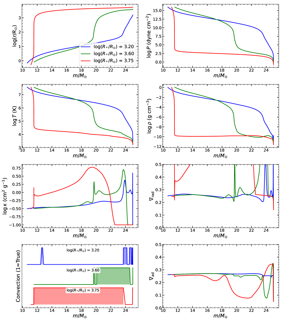
Figure 8: Profiles for $25\,M_{\odot}$ stars, similar to those in Figure 6, but with a minimum opacity floor of $\kappa\geq 0.1\,{\rm cm}^{2}\,{\rm g}^{-1}$. The blue, green, and red curves correspond to stellar radii of $\log(R_{*}/R_{\odot})=3.20$, 3.60, and 3.75, respectively, illustrating steady-state envelope solutions that roughly represent several time points as the star approaches the RSG phase. In the bottom-left panel, the color blocks represent the location of convective zones for different $R_{*}$.

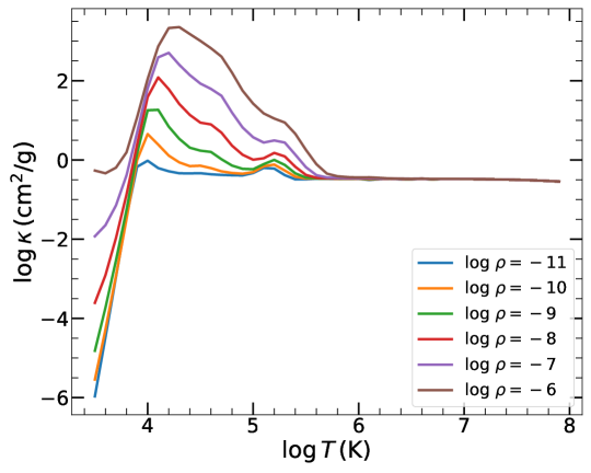
Figure 9: Opacity as a function of temperature for various densities retrieved from the MESA ”OP_gs98” opacity tables at $X=0.7$ and $Z=0.02$.

4.3 Red and Blue Solutions

Our envelope solutions provide insight into the distribution of giant and supergiant stars on the HR diagram. Based on the $R_{\rm in}$–$R_{*}$ and $R_{\rm in}$–$T_{\rm eff}$ relations shown in Figures 4 and 5, the solutions can be broadly divided into three distinct regimes:

(1) Red giant/supergiant phase: Near $T_{\rm eff}\sim 4,000\,{\rm K}$, the RG/RSG solution defines a limiting stellar radius and an effective temperature for envelope expansion. The RG/RSG configuration represents a distinct physical state, with an internal structure that differs fundamentally from that of stars with smaller radii. As a star approaches this regime, it undergoes a dramatic structural transition, characterized by substantial mass redistribution and the development of an extended convective envelope.

(2) Blue giant/supergiant regime: In the temperature range $T_{\rm eff}\sim 10,000$–$30,000\,{\rm K}$, a wide range of steady-state envelope solutions exist, determined primarily by $R_{\rm in}$, which is set by the core and H-burning shell properties. Generally, for a given luminosity, a smaller $R_{\rm in}$ corresponds to a larger $R_{*}$ within this blue regime.

(3) Yellow gap: Between $T_{\rm eff}\sim 4,000$–$10,000\,{\rm K}$, the $R_{\rm in}$ curves are nearly horizontal with respect to $R_{*}$ or $T_{\rm eff}$, indicating that only a small inward shift in $R_{\rm in}$ can cause the stellar radius to evolve significantly across this regime. This behavior is consistent with the observed Hertzsprung gap, where stars pass through quickly and few are observed in this temperature range. As a result, most giants and supergiants tend to converge either to the red or blue branches, rather than remaining in the yellow regime.

5 Discussions

Compared to full stellar evolution models, the advantage of our steady-state approach is that it allows us to explore all plausible combinations of physical quantities in stellar structures, rather than being restricted to specific evolutionary tracks. This flexibility enables us to isolate the problem from evolutionary effects and investigate the underlying physics that governs stellar envelope structures. Moreover, in stellar evolution simulations, modifying the opacity, surface boundary condition, or convection treatment often causes the computation to stall or fail. In contrast, steady-state models are not affected by prior evolutionary history and thus provide a more feasible framework to test a wide range of physical assumptions. Additionally, we solve only the envelope structure, defining the inner boundary using a constant pressure. This treatment allows us to focus specifically on the behavior of the envelope itself, and in particular, to examine the validity of the mirror principle within the realistic range of $M_{\rm in}$. By excluding the nuclear burning zones in the central region of the star, we also avoid the complexity arising from nuclear reactions.

Nevertheless, several limitations must be acknowledged. In our models, we assume a fixed luminosity throughout the envelope. This simplification allows us to avoid the gravothermal energy term, $\epsilon_{\rm grav}$, which depends on time derivatives and thus reflects the evolutionary history. However, as shown in Section 4, the input luminosity significantly influences the structure of the envelope. Because our steady-state models do not incorporate time evolution, they cannot determine which luminosity values correspond to actual stellar conditions. In fact, luminosity evolves substantially during the post-main-sequence stage. As shown in Paper I, the local luminosity at the base of the envelope correlates strongly with the radius at that point. Consequently, $R_{\rm in}$ and $L$ are coupled. In stellar evolution, a star does not follow a single $R_{\rm in}$–$R_{*}$ curve at fixed luminosity, as shown in Figures 4 and 5, but instead may traverse multiple such curves corresponding to various luminosities. Therefore, the relationship between $R_{\rm in}$ and $R_{*}$ derived from our constant luminosity models should be interpreted as general characteristics of the stellar structure, not as an evolutionary track. Furthermore, the full stellar structure requires solving both the core and the envelope self-consistently. Since our calculations omit the core, they do not include the structural constraints imposed by the core properties. To partially compensate for this, we use MESA stellar evolution models to guide the choice of inner boundary conditions and assess the validity of our envelope solutions. In summary, our approach has two main limitations. First, by adopting steady-state models to explore a wide range of structural configurations, we lose information about which configurations are realized in actual stellar evolution. Second, by isolating the envelope and excluding the core, we also lose the information about the physical constraints that arise from the core.

Despite these limitations, our method provides a powerful tool for understanding the fundamental physics of stellar envelopes. Beyond the application to RGs and RSGs presented in this paper, this approach can be extended to the study of other evolutionary phases, including advanced stages following core carbon burning.

6 Conclusions

To understand the physical origin of the mirror principle in envelope expansion and the distinct phase of RG/RSG in post-main-sequence evolution, we construct models of stellar envelopes to solve for steady-state solutions of their structures. These models allow us to explain three key features:

(1) The mirror principle for envelope expansion. Both realistic models and simplified polytropic models without energy treatment can generally reproduce the mirror principle in the regime of physically reasonable core masses: the inner and outer boundaries of the envelope move in the opposite directions. Therefore, this relationship is a natural consequence of the hydrostatic equilibrium regardless of energy transport. As the inner boundary of the envelope moves inward, its gravitational acceleration increases, requiring a steeper pressure gradient to maintain hydrostatic equilibrium. Since the pressure at this boundary is fixed by nuclear burning condition of the burning shell, the only way to achieve a steeper pressure gradient is to reduce the pressure and, therefore, the density in the outer envelope. As a result, the envelope expands in response to the contraction of the inner boundary of the envelope.

(2) The red giant/supergiant phase. The RG/RSG phase represents a distinct state in the stellar structure, characterized by significantly different temperature, density, and pressure profiles compared to stars with smaller radii. To reach this phase, a star undergoes a structural transition involving mass redistribution and the formation of an extended convective zone. Completion of this phase transition sets a limiting stellar radius and effective temperature ($\sim 4,000\,{\rm K}$). Once the star reaches this status, further inward motion of the envelope’s inner boundary no longer results in additional envelope expansion. The limiting extent of the stellar envelope is governed by a sharp decline in opacity as the temperature drops in the regime where H^- opacity dominates. The resulting reduction in opacity near the stellar surface flattens the temperature gradient, thereby altering the internal structure of the envelope. This physical limit on envelope expansion is consistent with the classical Hayashi limit.

(3) The Hertzsprung gap between blue and red regimes. Steady-state solutions show that a small change in the envelope’s inner boundary can drive the envelope to expand significantly across the yellow regime, corresponding to the temperature range of $\sim 4,000$-$10,000\,{\rm K}$. Therefore, stars tend to settle as either red or blue giants/supergiants, instead of remaining yellow. This behavior explains the bifurcation into red and blue supergiants revealed in the grid of stellar models (Ou et al., 2023), and accounts for the observed Hertzsprung gap in the HR diagram.

By combining these structural features revealed by steady-state envelope models with the evolutionary mechanisms presented in Paper I, we provide a comprehensive explanation for the long-standing question: why stars become red giants or supergiants.

References

- Hayashi & Hoshi (1961) Hayashi, C., & Hoshi, R. 1961, PASJ, 13, 442
- Iglesias & Rogers (1993) Iglesias, C. A., & Rogers, F. J. 1993, ApJ, 412, 752, doi: 10.1086/172958
- Iglesias & Rogers (1996) —. 1996, ApJ, 464, 943, doi: 10.1086/177381
- Jermyn et al. (2023) Jermyn, A. S., Bauer, E. B., Schwab, J., et al. 2023, ApJS, 265, 15, doi: 10.3847/1538-4365/acae8d
- Kippenhahn et al. (2013) Kippenhahn, R., Weigert, A., & Weiss, A. 2013, Stellar Structure and Evolution, doi: 10.1007/978-3-642-30304-3
- Ou & Chen (2024) Ou, P.-S., & Chen, K.-J. 2024, arXiv e-prints, arXiv:2407.21383, doi: 10.48550/arXiv.2407.21383
- Ou & Chen (2025) —. 2025, arXiv e-prints, arXiv:2506.01753. https://arxiv.org/abs/2506.01753
- Ou et al. (2023) Ou, P.-S., Chen, K.-J., Chu, Y.-H., & Tsai, S.-H. 2023, ApJ, 944, 34, doi: 10.3847/1538-4357/aca96e
- Paxton et al. (2011) Paxton, B., Bildsten, L., Dotter, A., et al. 2011, ApJS, 192, 3, doi: 10.1088/0067-0049/192/1/3
- Paxton et al. (2013) Paxton, B., Cantiello, M., Arras, P., et al. 2013, ApJS, 208, 4, doi: 10.1088/0067-0049/208/1/4
- Paxton et al. (2015) Paxton, B., Marchant, P., Schwab, J., et al. 2015, ApJS, 220, 15, doi: 10.1088/0067-0049/220/1/15
- Paxton et al. (2018) Paxton, B., Schwab, J., Bauer, E. B., et al. 2018, ApJS, 234, 34, doi: 10.3847/1538-4365/aaa5a8
- Paxton et al. (2019) Paxton, B., Smolec, R., Schwab, J., et al. 2019, ApJS, 243, 10, doi: 10.3847/1538-4365/ab2241
- Prialnik (2009) Prialnik, D. 2009, An Introduction to the Theory of Stellar Structure and Evolution
- Seaton (2005) Seaton, M. J. 2005, MNRAS, 362, L1, doi: 10.1111/j.1365-2966.2005.00019.x