Half-Iterates of x exp ( x ) x\exp(x) x + 1 / x x+1/x arcsinh ( x ) \operatorname{arcsinh}(x)
Steven Finch
(June 26, 2025)
Abstract
Given θ ( x ) \theta(x) g ( θ ( x ) ) = g ( x ) ± 1 g(\theta(x))=g(x)\pm 1 g ( x ) g(x) g ( x ) + δ g(x)+\delta δ \delta x x δ \delta δ \delta θ \theta
The Mavecha-Laohakosol [1 , 2 , 3 ] and Écalle-Jagy
[4 , 5 , 6 ] algorithms enable us to numerically solve
functional equations
g 6 ( x exp ( − x ) ) = g 6 ( x ) + 1 , x > 0 ; \begin{array}[c]{ccc}g_{6}\left(x\exp(-x)\right)=g_{6}(x)+1,&&x>0;\end{array}
g 7 ( W ( x ) ) = g 7 ( x ) − 1 , W ( x ) is Lambert’s function, x > 0 ; \begin{array}[c]{ccccc}g_{7}\left(W(x)\right)=g_{7}(x)-1,&&W(x)\text{ is Lambert's function,}&&x>0;\end{array}
g 8 ( x 1 + x 2 ) = g 8 ( x ) + 1 , x > 0 ; \begin{array}[c]{ccc}g_{8}\left(\dfrac{x}{1+x^{2}}\right)=g_{8}(x)+1,&&x>0;\end{array}
g 9 ( arcsinh ( x ) ) = g 9 ( x ) + 1 , arcsinh ( x ) = ln ( x + 1 + x 2 ) , x > 0 \begin{array}[c]{ccccc}g_{9}\left(\operatorname{arcsinh}(x)\right)=g_{9}(x)+1,&&\operatorname{arcsinh}(x)=\ln\left(x+\sqrt{1+x^{2}}\right),&&x>0\end{array}
in highly distinct ways. It is useful to have both methods available. For
both, the base function θ ( x ) \theta(x) θ ( 0 ) = 0 \theta(0)=0 θ ′ ( 0 ) = 1 \theta^{\prime}(0)=1
x + ∑ m = 1 ∞ c m x m τ + 1 , c 1 = γ < 0 , τ ≥ 1 is an integer. \begin{array}[c]{ccccc}x+{\displaystyle\sum\limits_{m=1}^{\infty}}c_{m}x^{m\,\tau+1},&&c_{1}=\gamma<0,&&\tau\geq 1\text{ is an integer.}\end{array}
In words, θ ( x ) \theta(x) x = 0 x=0 τ \tau g ( x ) g(x) λ ( x ) \lambda(x)
λ ( θ ( x ) ) = θ ′ ( x ) λ ( x ) \lambda(\theta(x))=\theta^{\prime}(x)\lambda(x)
whose reciprocal approximates the derivative g ′ ( x ) g^{\prime}(x) g ( x ) g(x) g ( x ) + δ g(x)+\delta δ \delta δ \delta
Let us review the first & third examples from [6 ] , in the
interest of clarity. Given θ 1 ( x ) = x ( 1 − x ) \theta_{1}(x)=x(1-x)
g 1 ( x ) \displaystyle g_{1}(x) = 1 x + ln ( x ) + 1 2 x + 1 3 x 2 + 13 36 x 3 + 113 240 x 4 + 1187 1800 x 5 + 877 945 x 6 \displaystyle=\frac{1}{x}+\ln(x)+\frac{1}{2}x+\frac{1}{3}x^{2}+\frac{13}{36}x^{3}+\frac{113}{240}x^{4}+\frac{1187}{1800}x^{5}+\frac{877}{945}x^{6}
+ 14569 11760 x 7 + 176017 120960 x 8 + 1745717 1360800 x 9 + 88217 259875 x 10 \displaystyle+\frac{14569}{11760}x^{7}+\frac{176017}{120960}x^{8}+\frac{1745717}{1360800}x^{9}+\frac{88217}{259875}x^{10}
− 147635381 109771200 x 11 − 3238110769 1556755200 x 12 + ⋯ . \displaystyle-\frac{147635381}{109771200}x^{11}-\frac{3238110769}{1556755200}x^{12}+\cdots.
To actually calculate g 1 ( x ) g_{1}(x) 0 < x < 1 0<x<1 x 0 = x x_{0}=x x n = x n − 1 ( 1 − x n − 1 ) x_{n}=x_{n-1}(1-x_{n-1}) n ≥ 1 n\geq 1 g 1 ( x ) g_{1}(x)
g 1 ( x ) = lim n → ∞ [ g 1 ( x n ) − n ] . g_{1}(x)=\lim_{n\rightarrow\infty}\,\left[g_{1}(x_{n})-n\right].
For example, to 100 decimal digits of accuracy,
g 1 ( 1 2 ) \displaystyle g_{1}\left(\frac{1}{2}\right) = 1.76799378613615405044363440678113233107768143313195 \ \displaystyle=1.76799378613615405044363440678113233107768143313195\backslash
65155769860596260007646063875144448165163256825025 … . \displaystyle\;\;\;\;\;\;\;\;65155769860596260007646063875144448165163256825025....
ML allows calculation of
g ~ 1 ( x ) = − lim n → ∞ n 2 ( x n − 1 n + ln ( n ) n 2 ) \tilde{g}_{1}(x)=-\lim_{n\rightarrow\infty}n^{2}\left(x_{n}-\frac{1}{n}+\frac{\ln(n)}{n^{2}}\right)
to high precision and it seems that g 1 ( 1 / 2 ) = g_{1}(1/2)= g ~ 1 ( 1 / 2 ) \tilde{g}_{1}\left(1/2\right) δ 1 = 0 \delta_{1}=0 x = x 0 x=x_{0}
Given θ 3 ( x ) = sin ( x ) \theta_{3}(x)=\sin(x)
g 3 ( x ) \displaystyle g_{3}(x) = 3 x 2 + 6 5 ln ( x ) + 79 1050 x 2 + 29 2625 x 4 + 91543 36382500 x 6 + 18222899 28378350000 x 8 \displaystyle=\frac{3}{x^{2}}+\frac{6}{5}\ln(x)+\frac{79}{1050}x^{2}+\frac{29}{2625}x^{4}+\frac{91543}{36382500}x^{6}+\frac{18222899}{28378350000}x^{8}
+ 88627739 573024375000 x 10 + 3899439883 142468185234375 x 12 − 32544553328689 116721334798818750000 x 14 − ⋯ . \displaystyle+\frac{88627739}{573024375000}x^{10}+\frac{3899439883}{142468185234375}x^{12}-\frac{32544553328689}{116721334798818750000}x^{14}-\cdots.
To actually calculate g 3 ( x ) g_{3}(x) 0 < x < π 0<x<\pi x 0 = x x_{0}=x x n = sin ( x n − 1 ) x_{n}=\sin(x_{n-1}) n ≥ 1 n\geq 1
g 3 ( x ) = lim n → ∞ [ g 3 ( x n ) − n ] . g_{3}(x)=\lim_{n\rightarrow\infty}\,\left[g_{3}(x_{n})-n\right].
For example [7 ] ,
g 3 ( π 2 ) \displaystyle g_{3}\left(\frac{\pi}{2}\right) = 2.08962271972954305953784727641750978539901952044337 \ \displaystyle=2.08962271972954305953784727641750978539901952044337\backslash
62593345954823058366250507039441172654894541567102 … . \displaystyle\;\;\;\;\;\;\;\;62593345954823058366250507039441172654894541567102....
ML permits calculation of
g ~ 3 ( x ) = − lim n → ∞ 2 n 3 / 2 ( x n 3 − 1 n 1 / 2 + 3 10 ln ( n ) n 3 / 2 ) \tilde{g}_{3}(x)=-\lim_{n\rightarrow\infty}2n^{3/2}\left(\frac{x_{n}}{\sqrt{3}}-\frac{1}{n^{1/2}}+\frac{3}{10}\frac{\ln(n)}{n^{3/2}}\right)
to high precision and, in contrast [7 ] ,
g ~ 3 ( π 2 ) \displaystyle\tilde{g}_{3}\left(\frac{\pi}{2}\right) = 1.43045534652867724470070013426399436261052518574972 \ \displaystyle=1.43045534652867724470070013426399436261052518574972\backslash
65882937788821233400491195385639930960365659174569 … . \displaystyle\;\;\;\;\;\;\;\;65882937788821233400491195385639930960365659174569....
The difference between the EJ-based & ML-based values is nonzero and
conjectured to be
δ 3 = g 3 ( π / 2 ) − g ~ 3 ( π / 2 ) = ( 3 / 5 ) ln ( 3 ) . \delta_{3}=g_{3}\left(\pi/2\right)-\tilde{g}_{3}\left(\pi/2\right)=(3/5)\ln(3).
Similarly, for θ 5 ( x ) = ln ( 1 + x ) \theta_{5}(x)=\ln(1+x) x > 0 x>0
δ 5 = g 5 ( 1 ) − g ~ 5 ( 1 ) = ( 1 / 3 ) ln ( 2 ) . \delta_{5}=g_{5}\left(1\right)-\tilde{g}_{5}\left(1\right)=(1/3)\ln(2)\text{.}
These identities should hold for any choice of x = x 0 x=x_{0}
For suitably large integer K K
φ K ( x ) = x + ∑ m = 1 K c m x m τ + 1 , ψ K ( x ) = φ K + 1 ′ ( x ) \begin{array}[c]{ccc}\varphi_{K}(x)=x+{\displaystyle\sum\limits_{m=1}^{K}}c_{m}x^{m\,\tau+1},&&\psi_{K}(x)=\varphi_{K+1}^{\prime}(x)\end{array}
(omit the subscript K K
Set v 1 = a , L ( x ) = γ φ ( x ) τ + 1 , R ( x ) = γ x τ + 1 For k = 3 to K − 1 L ( x ) ⟵ L ( x ) + ( v k − 2 − a ) φ ( x ) ε ( − 1 , k ) + a φ ( x ) ε ( 0 , k ) R ( x ) ⟵ R ( x ) + ( v k − 2 − a ) x ε ( − 1 , k ) + a x ε ( 0 , k ) Solve [ x ε ( 1 , k ) ] { L ( x ) − ψ ( x ) R ( x ) } = 0 for unknown a v k − 1 ⟵ a Clear a End For Set λ K ( x ) = γ x τ + 1 + ∑ m = 2 K − 2 v m x τ m + 1 \begin{array}[c]{ll}\text{Set}&v_{1}=a,\;\;\;L(x)=\gamma\,\varphi(x)^{\tau+1},\;\;\;R(x)=\gamma\,x^{\tau+1}\vskip 3.0pt plus 1.0pt minus 1.0pt\\
\text{For}&k=3\text{ to }K-1\vskip 3.0pt plus 1.0pt minus 1.0pt\\
&L(x)\longleftarrow L(x)+\left(v_{k-2}-a\right)\varphi(x)^{\varepsilon(-1,k)}+a\,\varphi(x)^{\varepsilon(0,k)}\vskip 3.0pt plus 1.0pt minus 1.0pt\\
&R(x)\longleftarrow R(x)+\left(v_{k-2}-a\right)x^{\varepsilon(-1,k)}+a\,x^{\varepsilon(0,k)}\vskip 3.0pt plus 1.0pt minus 1.0pt\\
&\text{Solve }\left[x^{\varepsilon(1,k)}\right]\left\{L(x)-\psi(x)R(x)\right\}=0\text{ for unknown }a\vskip 3.0pt plus 1.0pt minus 1.0pt\\
&v_{k-1}\longleftarrow a\vskip 3.0pt plus 1.0pt minus 1.0pt\\
&\text{Clear }a\vskip 3.0pt plus 1.0pt minus 1.0pt\\
\text{End}&\text{For}\\
\text{Set}&\lambda_{K}(x)=\gamma\,x^{\tau+1}+{\displaystyle\sum\limits_{m=2}^{K-2}}v_{m}x^{\tau\,m+1}\end{array}
where
ε ( j , k ) = τ ( j + k − 1 ) + 1 \varepsilon(j,k)=\tau\left(j+k-1\right)+1
and [ x n ] { f ( x ) } [x^{n}]\{f(x)\} x n x^{n} f ( x ) f(x) [8 ] . This algorithm is
described in greater depth in [6 , 9 ] .
The issue of g ( x ) g(x) g ( x ) + δ g(x)+\delta
1 𝜽 6 ( 𝒙 ) = 𝒙 exp ( − 𝒙 ) \boldsymbol{\theta}_{6}\boldsymbol{(x)=x}\exp\boldsymbol{(-x)}
Our starting point is τ = 1 \tau=1 γ = − 1 \gamma=-1
{ ε ( − 1 , k ) , ε ( 0 , k ) , ε ( 1 , k ) } = { k − 1 , k , k + 1 } . \left\{\varepsilon(-1,k),\varepsilon(0,k),\varepsilon(1,k)\right\}=\left\{k-1,k,k+1\right\}.
We initialize:
φ ( x ) = x − x 2 + 1 2 x 3 − 1 6 x 4 + 1 24 x 5 − 1 120 x 6 + 1 720 x 7 − 1 5040 x 8 + 1 40320 x 9 − ⋯ , \varphi(x)=x-x^{2}+\frac{1}{2}x^{3}-\frac{1}{6}x^{4}+\frac{1}{24}x^{5}-\frac{1}{120}x^{6}+\frac{1}{720}x^{7}-\frac{1}{5040}x^{8}+\frac{1}{40320}x^{9}-\cdots,
ψ ( x ) = 1 − 2 x + 3 2 x 2 − 2 3 x 3 + 5 24 x 4 − 1 20 x 5 + 7 720 x 6 − 1 630 x 7 + 1 4480 x 8 − 1 36288 x 9 + ⋯ , \psi(x)=1-2x+\frac{3}{2}x^{2}-\frac{2}{3}x^{3}+\frac{5}{24}x^{4}-\frac{1}{20}x^{5}+\frac{7}{720}x^{6}-\frac{1}{630}x^{7}+\frac{1}{4480}x^{8}-\frac{1}{36288}x^{9}+\cdots,
v 1 = a , L ( x ) = − φ ( x ) 2 , R ( x ) = − x 2 \begin{array}[c]{ccccc}v_{1}=a,&&L(x)=-\varphi(x)^{2},&&R(x)=-x^{2}\end{array}
where a a k = 3 k=3
L ( x ) ⟵ L ( x ) + 0 + a φ ( x ) 3 = − φ ( x ) 2 + a φ ( x ) 3 , L(x)\longleftarrow L(x)+0+a\,\varphi(x)^{3}=-\varphi(x)^{2}+a\,\varphi(x)^{3},
R ( x ) ⟵ R ( x ) + 0 + a x 3 = − x 2 + a x 3 R(x)\longleftarrow R(x)+0+a\,x^{3}=-x^{2}+a\,x^{3}
and extract the coefficient of x 4 x^{4}
L ( x ) − ψ ( x ) R ( x ) = − φ ( x ) 2 + a φ ( x ) 3 − ψ ( x ) ( − x 2 + a x 3 ) . L(x)-\psi(x)R(x)=-\varphi(x)^{2}+a\,\varphi(x)^{3}-\psi(x)\left(-x^{2}+a\,x^{3}\right).
Computer algebra gives this coefficient to be − 1 / 2 − a -1/2-a a = − 1 / 2 a=-1/2 v 2 = − 1 / 2 v_{2}=-1/2 a a k = 4 k=4
L ( x ) ⟵ L ( x ) + ( − 1 / 2 − a ) φ ( x ) 3 + a φ ( x ) 4 = − φ ( x ) 2 + ( − 1 / 2 ) φ ( x ) 3 + a φ ( x ) 4 , L(x)\longleftarrow L(x)+\left(-1/2-a\right)\varphi(x)^{3}+a\,\varphi(x)^{4}=-\varphi(x)^{2}+(-1/2)\varphi(x)^{3}+a\,\varphi(x)^{4},
R ( x ) ⟵ R ( x ) + ( − 1 / 2 − a ) x 3 + a x 4 = − x 2 + ( − 1 / 2 ) x 3 + a x 4 R(x)\longleftarrow R(x)+\left(-1/2-a\right)x^{3}+a\,x^{4}=-x^{2}+(-1/2)x^{3}+a\,x^{4}
and extract the coefficient of x 5 x^{5}
L ( x ) − ψ ( x ) R ( x ) = − φ ( x ) 2 − ( 1 / 2 ) φ ( x ) 3 + a φ ( x ) 4 − ψ ( x ) ( − x 2 − ( 1 / 2 ) x 3 + a x 4 ) . L(x)-\psi(x)R(x)=-\varphi(x)^{2}-(1/2)\varphi(x)^{3}+a\,\varphi(x)^{4}-\psi(x)\left(-x^{2}-(1/2)x^{3}+a\,x^{4}\right).
Computer algebra gives this coefficient to be − 5 / 6 − 2 a -5/6-2a a = − 5 / 12 a=-5/12 v 3 = − 5 / 12 v_{3}=-5/12 a a k = 5 k=5
λ ( x ) \displaystyle\lambda(x) = − x 2 − 1 2 x 3 − 5 12 x 4 − 5 12 x 5 − 107 240 x 6 − 173 360 x 7 − 7577 15120 x 8 − 14867 30240 x 9 \displaystyle=-x^{2}-\frac{1}{2}x^{3}-\frac{5}{12}x^{4}-\frac{5}{12}x^{5}-\frac{107}{240}x^{6}-\frac{173}{360}x^{7}-\frac{7577}{15120}x^{8}-\frac{14867}{30240}x^{9}
− 36461 80640 x 10 − 41891 100800 x 11 − 493013 1108800 x 12 − ⋯ \displaystyle-\frac{36461}{80640}x^{10}-\frac{41891}{100800}x^{11}-\frac{493013}{1108800}x^{12}-\cdots
hence
g 6 ′ ( x ) \displaystyle g_{6}^{\prime}(x) = 1 λ ( x ) = − 1 x 2 + 1 2 x + 1 6 + 1 8 x + 19 180 x 2 + 1 12 x 3 + 41 840 x 4 + 37 17280 x 5 \displaystyle=\frac{1}{\lambda(x)}=-\frac{1}{x^{2}}+\frac{1}{2x}+\frac{1}{6}+\frac{1}{8}x+\frac{19}{180}x^{2}+\frac{1}{12}x^{3}+\frac{41}{840}x^{4}+\frac{37}{17280}x^{5}
− 18349 453600 x 6 − 443 10080 x 7 + 55721 2395008 x 8 + 84317 691200 x 9 + 2594833561 36324288000 x 10 \displaystyle-\frac{18349}{453600}x^{6}-\frac{443}{10080}x^{7}+\frac{55721}{2395008}x^{8}+\frac{84317}{691200}x^{9}+\frac{2594833561}{36324288000}x^{10}
− 152043613 479001600 x 11 − 830066563 1334361600 x 12 + ⋯ \displaystyle-\frac{152043613}{479001600}x^{11}-\frac{830066563}{1334361600}x^{12}+\cdots
hence the Abel solution is
g 6 ( x ) \displaystyle g_{6}(x) = 1 x + 1 2 ln ( x ) + 1 6 x + 1 16 x 2 + 19 540 x 3 + 1 48 x 4 + 41 4200 x 5 + 37 103680 x 6 \displaystyle=\frac{1}{x}+\frac{1}{2}\ln(x)+\frac{1}{6}x+\frac{1}{16}x^{2}+\frac{19}{540}x^{3}+\frac{1}{48}x^{4}+\frac{41}{4200}x^{5}+\frac{37}{103680}x^{6}
− 18349 3175200 x 7 − 443 80640 x 8 + 55721 21555072 x 9 + 84317 6912000 x 10 \displaystyle-\frac{18349}{3175200}x^{7}-\frac{443}{80640}x^{8}+\frac{55721}{21555072}x^{9}+\frac{84317}{6912000}x^{10}
+ 2594833561 399567168000 x 11 − 152043613 5748019200 x 12 − ⋯ . \displaystyle+\frac{2594833561}{399567168000}x^{11}-\frac{152043613}{5748019200}x^{12}-\cdots.
To actually calculate g 6 ( x ) g_{6}(x) x > 0 x>0 x 0 = x x_{0}=x x n = x n − 1 exp ( − x n − 1 ) x_{n}=x_{n-1}\exp(-x_{n-1}) n ≥ 1 n\geq 1 g 6 ( x ) g_{6}(x)
g 6 ( x ) = lim n → ∞ [ g 6 ( x n ) − n ] . g_{6}(x)=\lim_{n\rightarrow\infty}\,\left[g_{6}(x_{n})-n\right].
For example [3 ] ,
g 6 ( 1 2 ) \displaystyle g_{6}\left(\frac{1}{2}\right) = 1.75834255858972372062643806210115977597027119625090 \ \displaystyle=1.75834255858972372062643806210115977597027119625090\backslash
80917543312980057047235243525304830956768215851070 … \displaystyle\;\;\;\;\;\;\;80917543312980057047235243525304830956768215851070...
g 6 ( 1 ) \displaystyle g_{6}(1) = 1.29024720868776429166761568416118463727576441467337 \ \displaystyle=1.29024720868776429166761568416118463727576441467337\backslash
27282792783387848274298261878073817117283133623657 … , \displaystyle\;\;\;\;\;\;\;27282792783387848274298261878073817117283133623657...,
g 6 ( 3 2 ) \displaystyle g_{6}\left(\frac{3}{2}\right) = 1.50492798428335150009539332223367713135060756851783 \ \displaystyle=1.50492798428335150009539332223367713135060756851783\backslash
70693140248668083561715772083535204539601724490351 … \displaystyle\;\;\;\;\;\;\;70693140248668083561715772083535204539601724490351...
computed using both EJ and ML. In this case, the two methods agree perfectly
and evidently δ 6 = 0 \delta_{6}=0
2 𝜽 7 ( 𝒙 ) = 𝑾 ( 𝒙 ) \boldsymbol{\theta}_{7}\boldsymbol{(x)=W(x)}
In order for critical hypotheses to be met, we examine not x exp ( x ) x\exp(x) W ( x ) W(x) τ = 1 \tau=1 γ = − 1 \gamma=-1 ε ( j , k ) \varepsilon(j,k)
φ ( x ) = x − x 2 + 3 2 x 3 − 8 3 x 4 + 125 24 x 5 − 54 5 x 6 + 16807 720 x 7 − 16384 315 x 8 + 531441 4480 x 9 − ⋯ , \varphi(x)=x-x^{2}+\frac{3}{2}x^{3}-\frac{8}{3}x^{4}+\frac{125}{24}x^{5}-\frac{54}{5}x^{6}+\frac{16807}{720}x^{7}-\frac{16384}{315}x^{8}+\frac{531441}{4480}x^{9}-\cdots,
ψ ( x ) = 1 − 2 x + 9 2 x 2 − 32 3 x 3 + 625 24 x 4 − 324 5 x 5 + 117649 720 x 6 − 131072 315 x 7 + 4782969 4480 x 8 − ⋯ , \psi(x)=1-2x+\frac{9}{2}x^{2}-\frac{32}{3}x^{3}+\frac{625}{24}x^{4}-\frac{324}{5}x^{5}+\frac{117649}{720}x^{6}-\frac{131072}{315}x^{7}+\frac{4782969}{4480}x^{8}-\cdots,
v 1 = a , L ( x ) = − φ ( x ) 2 , R ( x ) = − x 2 \begin{array}[c]{ccccc}v_{1}=a,&&L(x)=-\varphi(x)^{2},&&R(x)=-x^{2}\end{array}
where a a k = 3 k=3
L ( x ) ⟵ L ( x ) + 0 + a φ ( x ) 3 = − φ ( x ) 2 + a φ ( x ) 3 , L(x)\longleftarrow L(x)+0+a\,\varphi(x)^{3}=-\varphi(x)^{2}+a\,\varphi(x)^{3},
R ( x ) ⟵ R ( x ) + 0 + a x 3 = − x 2 + a x 3 R(x)\longleftarrow R(x)+0+a\,x^{3}=-x^{2}+a\,x^{3}
and extract the coefficient of x 4 x^{4}
L ( x ) − ψ ( x ) R ( x ) = − φ ( x ) 2 + a φ ( x ) 3 − ψ ( x ) ( − x 2 + a x 3 ) . L(x)-\psi(x)R(x)=-\varphi(x)^{2}+a\,\varphi(x)^{3}-\psi(x)\left(-x^{2}+a\,x^{3}\right).
Computer algebra gives this coefficient to be 1 / 2 − a 1/2-a a = 1 / 2 a=1/2 v 2 = 1 / 2 v_{2}=1/2 a a k = 4 k=4
L ( x ) ⟵ L ( x ) + ( 1 / 2 − a ) φ ( x ) 3 + a φ ( x ) 4 = − φ ( x ) 2 + ( 1 / 2 ) φ ( x ) 3 + a φ ( x ) 4 , L(x)\longleftarrow L(x)+\left(1/2-a\right)\varphi(x)^{3}+a\,\varphi(x)^{4}=-\varphi(x)^{2}+(1/2)\varphi(x)^{3}+a\,\varphi(x)^{4},
R ( x ) ⟵ R ( x ) + ( 1 / 2 − a ) x 3 + a x 4 = − x 2 + ( 1 / 2 ) x 3 + a x 4 R(x)\longleftarrow R(x)+\left(1/2-a\right)x^{3}+a\,x^{4}=-x^{2}+(1/2)x^{3}+a\,x^{4}
and extract the coefficient of x 5 x^{5}
L ( x ) − ψ ( x ) R ( x ) = − φ ( x ) 2 + ( 1 / 2 ) φ ( x ) 3 + a φ ( x ) 4 − ψ ( x ) ( − x 2 + ( 1 / 2 ) x 3 + a x 4 ) . L(x)-\psi(x)R(x)=-\varphi(x)^{2}+(1/2)\varphi(x)^{3}+a\,\varphi(x)^{4}-\psi(x)\left(-x^{2}+(1/2)x^{3}+a\,x^{4}\right).
Computer algebra gives this coefficient to be − 5 / 6 − 2 a -5/6-2a a = − 5 / 12 a=-5/12 v 3 = − 5 / 12 v_{3}=-5/12 a a k = 5 k=5
λ ( x ) \displaystyle\lambda(x) = − x 2 + 1 2 x 3 − 5 12 x 4 + 5 12 x 5 − 107 240 x 6 + 173 360 x 7 − 7577 15120 x 8 + 14867 30240 x 9 \displaystyle=-x^{2}+\frac{1}{2}x^{3}-\frac{5}{12}x^{4}+\frac{5}{12}x^{5}-\frac{107}{240}x^{6}+\frac{173}{360}x^{7}-\frac{7577}{15120}x^{8}+\frac{14867}{30240}x^{9}
− 36461 80640 x 10 + 41891 100800 x 11 − 493013 1108800 x 12 + ⋯ \displaystyle-\frac{36461}{80640}x^{10}+\frac{41891}{100800}x^{11}-\frac{493013}{1108800}x^{12}+\cdots
hence
− g 7 ′ ( x ) \displaystyle-g_{7}^{\prime}(x) = 1 λ ( x ) = − 1 x 2 − 1 2 x + 1 6 − 1 8 x + 19 180 x 2 − 1 12 x 3 + 41 840 x 4 − 37 17280 x 5 \displaystyle=\frac{1}{\lambda(x)}=-\frac{1}{x^{2}}-\frac{1}{2x}+\frac{1}{6}-\frac{1}{8}x+\frac{19}{180}x^{2}-\frac{1}{12}x^{3}+\frac{41}{840}x^{4}-\frac{37}{17280}x^{5}
− 18349 453600 x 6 + 443 10080 x 7 + 55721 2395008 x 8 − 84317 691200 x 9 + 2594833561 36324288000 x 10 \displaystyle-\frac{18349}{453600}x^{6}+\frac{443}{10080}x^{7}+\frac{55721}{2395008}x^{8}-\frac{84317}{691200}x^{9}+\frac{2594833561}{36324288000}x^{10}
+ 152043613 479001600 x 11 − 830066563 1334361600 x 12 − ⋯ \displaystyle+\frac{152043613}{479001600}x^{11}-\frac{830066563}{1334361600}x^{12}-\cdots
hence
− g 7 ( x ) \displaystyle-g_{7}(x) = 1 x − 1 2 ln ( x ) + 1 6 x − 1 16 x 2 + 19 540 x 3 − 1 48 x 4 + 41 4200 x 5 − 37 103680 x 6 \displaystyle=\frac{1}{x}-\frac{1}{2}\ln(x)+\frac{1}{6}x-\frac{1}{16}x^{2}+\frac{19}{540}x^{3}-\frac{1}{48}x^{4}+\frac{41}{4200}x^{5}-\frac{37}{103680}x^{6}
− 18349 3175200 x 7 + 443 80640 x 8 + 55721 21555072 x 9 − 84317 6912000 x 10 \displaystyle-\frac{18349}{3175200}x^{7}+\frac{443}{80640}x^{8}+\frac{55721}{21555072}x^{9}-\frac{84317}{6912000}x^{10}
+ 2594833561 399567168000 x 11 + 152043613 5748019200 x 12 − ⋯ . \displaystyle+\frac{2594833561}{399567168000}x^{11}+\frac{152043613}{5748019200}x^{12}-\cdots.
To actually calculate − g 7 ( x ) -g_{7}(x) x > 0 x>0 x 0 = x x_{0}=x x n = W ( x n − 1 ) x_{n}=W(x_{n-1}) n ≥ 1 n\geq 1 g 7 ( x ) g_{7}(x)
− g 7 ( x ) = lim n → ∞ [ − g 7 ( x n ) − n ] . -g_{7}(x)=\lim_{n\rightarrow\infty}\,\left[-g_{7}(x_{n})-n\right].
Clearly g 7 ( x exp ( x ) ) = g 7 ( x ) + 1 g_{7}(x\exp(x))=g_{7}(x)+1
g 7 ( 1 ) \displaystyle g_{7}(1) = 1.12598177657449557838525587897615642800725150980305 \ \displaystyle=1.12598177657449557838525587897615642800725150980305\backslash
63945245583299478474227705427041049529141887963750 … , \displaystyle\;\;\;\;\;\;\;\;63945245583299478474227705427041049529141887963750...,
g 7 ( 4 ) \displaystyle g_{7}(4) = − 0.11499372373410084169182378714739554828282610037248 \ \displaystyle=-0.11499372373410084169182378714739554828282610037248\backslash
21296567880346223422503807018752834650657738379829 … . \displaystyle\;\;\;\;\;\;\;\;\;\;\;21296567880346223422503807018752834650657738379829....
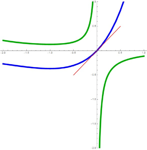
The connection between solutions of
f ( x exp ( x ) ) = f ( x ) + 1 , x ≠ 0 \begin{array}[c]{ccc}f(x\exp(x))=f(x)+1,&&x\neq 0\end{array}
and our work above lies in the formula f = f 67 f=f_{67}
f 67 ( x ) = { g 6 ( − x ) if x < 0 , − g 7 ( x ) if x > 0 . f_{67}(x)=\left\{\begin{array}[c]{lll}g_{6}(-x)&&\text{if }x<0,\\
-g_{7}(x)&&\text{if }x>0.\end{array}\right.
As pictured in Figure 1, the Abel solutions are each analytic but neither one
is a continuation of the other. According to [10 ] , each
λ ( x ) \lambda(x) [11 ] for an alterative treatment.
3 𝒙 + 𝟏 / 𝒙 \boldsymbol{x+1/x} 𝜽 8 ( 𝒚 ) = 𝒚 / ( 𝟏 + 𝒚 2 ) \boldsymbol{\theta}_{8}\boldsymbol{(y)=y/(1+y}^{2})
ML cannot be applied to x + 1 / x x+1/x
1 x + 1 / x | x = 1 / y = 1 1 / y + y = y 1 + y 2 \left.\frac{1}{x+1/x}\right|_{x=1/y}=\frac{1}{1/y+y}=\frac{y}{1+y^{2}}
and [12 ]
− lim n → ∞ 2 n 3 / 2 ( 2 1 / 2 y n − 1 n 1 / 2 + 1 8 ln ( n ) n 3 / 2 ) = g ~ 8 ( y ) , -\lim_{n\rightarrow\infty}2n^{3/2}\left(2^{1/2}y_{n}-\frac{1}{n^{1/2}}+\frac{1}{8}\frac{\ln(n)}{n^{3/2}}\right)=\tilde{g}_{8}(y),
lim n → ∞ n 1 / 2 ( 2 1 / 2 x n − 2 n 1 / 2 − 1 4 ln ( n ) n 1 / 2 ) = g ~ 8 ( 1 x ) \lim_{n\rightarrow\infty}n^{1/2}\left(2^{1/2}x_{n}-2n^{1/2}-\frac{1}{4}\frac{\ln(n)}{n^{1/2}}\right)=\tilde{g}_{8}\left(\frac{1}{x}\right)
where
y = y 0 > 0 , y n = y n − 1 / ( 1 + y n − 1 2 ) ; \begin{array}[c]{ccc}y=y_{0}>0,&&y_{n}=y_{n-1}/\left(1+y_{n-1}^{2}\right);\end{array}
x = x 0 = 1 / y 0 , x n = x n − 1 + 1 / x n − 1 . \begin{array}[c]{ccc}x=x_{0}=1/y_{0},&&x_{n}=x_{n-1}+1/x_{n-1}.\end{array}
Turning attention to EJ, we have τ = 2 \tau=2 γ = − 1 \gamma=-1
{ ε ( − 1 , k ) , ε ( 0 , k ) , ε ( 1 , k ) } = { 2 k − 3 , 2 k − 1 , 2 k + 1 } . \left\{\varepsilon(-1,k),\varepsilon(0,k),\varepsilon(1,k)\right\}=\left\{2k-3,2k-1,2k+1\right\}.
Omitting details, we obtain
λ ( y ) \displaystyle\lambda(y) = − y 3 − 1 2 y 5 − 1 2 y 7 − 7 12 y 9 − 2 3 y 11 − 13 20 y 13 − 9 20 y 15 \displaystyle=-y^{3}-\frac{1}{2}y^{5}-\frac{1}{2}y^{7}-\frac{7}{12}y^{9}-\frac{2}{3}y^{11}-\frac{13}{20}y^{13}-\frac{9}{20}y^{15}
− 71 280 y 17 − 121 140 y 19 − 19 7 y 21 − 11 20 y 23 + 171569 9240 y 25 + ⋯ \displaystyle-\frac{71}{280}y^{17}-\frac{121}{140}y^{19}-\frac{19}{7}y^{21}-\frac{11}{20}y^{23}+\frac{171569}{9240}y^{25}+\cdots
hence
g 8 ( y ) \displaystyle g_{8}(y) = 1 2 y 2 + 1 2 ln ( y ) + 1 8 y 2 + 5 96 y 4 + 7 288 y 6 − 1 1280 y 8 − 671 28800 y 10 − 9607 483840 y 12 \displaystyle=\frac{1}{2y^{2}}+\frac{1}{2}\ln(y)+\frac{1}{8}y^{2}+\frac{5}{96}y^{4}+\frac{7}{288}y^{6}-\frac{1}{1280}y^{8}-\frac{671}{28800}y^{10}-\frac{9607}{483840}y^{12}
+ 10187 225792 y 14 + 954907 7741440 y 16 − 10382759 87091200 y 18 − 299685973 304128000 y 20 \displaystyle+\frac{10187}{225792}y^{14}+\frac{954907}{7741440}y^{16}-\frac{10382759}{87091200}y^{18}-\frac{299685973}{304128000}y^{20}
+ 684110137 14050713600 y 22 + 171403792979 15941173248 y 24 + ⋯ . \displaystyle+\frac{684110137}{14050713600}y^{22}+\frac{171403792979}{15941173248}y^{24}+\cdots.
For example,
g 8 ( 1 ) \displaystyle g_{8}\left(1\right) = 0.68828439242872540317747334422366915982213509764617 \ \displaystyle=0.68828439242872540317747334422366915982213509764617\backslash
93168899434154492265236034277589425850733342338149 … , \displaystyle\;\;\;\;\;\;\;\;93168899434154492265236034277589425850733342338149...,
g 8 ( 3 ) \displaystyle g_{8}\left(3\right) = 3.96525855036809341124152686622098713140662994958412 \ \displaystyle=3.96525855036809341124152686622098713140662994958412\backslash
78202764290285396844369745309712979065528562981062 … \displaystyle\;\;\;\;\;\;\;\;78202764290285396844369745309712979065528562981062...
computed using EJ and
g 8 ( y ) = lim n → ∞ [ g 8 ( y n ) − n ] . g_{8}\left(y\right)=\lim_{n\rightarrow\infty}\,\left[g_{8}(y_{n})-n\right].
These quantities differ from ML-based estimates by a nonzero constant,
conjectured to be
δ 8 = g 8 ( y ) − g ~ 8 ( y ) = − ( 1 / 4 ) ln ( 2 ) \delta_{8}=g_{8}\left(y\right)-\tilde{g}_{8}\left(y\right)=-(1/4)\ln(2)
e.g., the Abel solution at 1 1
g ~ 8 ( 1 ) \displaystyle\tilde{g}_{8}\left(1\right) = 0.86157118756871173053178137458821330184101013123624 \ \displaystyle=0.86157118756871173053178137458821330184101013123624\backslash
31304201134178225749290958514378440509050833384868 … . \displaystyle\;\;\;\;\;\;\;\;31304201134178225749290958514378440509050833384868....
References to the literature about x n = x n − 1 + 1 / x n − 1 x_{n}=x_{n-1}+1/x_{n-1} [12 ] , as well as the value g ~ 8 ( 1 ) \tilde{g}_{8}\left(1\right) δ 8 < 0 \delta_{8}<0
4 𝜽 9 ( 𝒙 ) = arcsinh ( 𝒙 ) \boldsymbol{\theta}_{9}\boldsymbol{(x)=}\operatorname{arcsinh}\boldsymbol{(x)}
This section is included mostly as a companion to our discussion of sin ( x ) \sin(x) [6 ] . Here τ = 2 \tau=2 γ = − 1 / 6 \gamma=-1/6
{ ε ( − 1 , k ) , ε ( 0 , k ) , ε ( 1 , k ) } = { 2 k − 3 , 2 k − 1 , 2 k + 1 } . \left\{\varepsilon(-1,k),\varepsilon(0,k),\varepsilon(1,k)\right\}=\left\{2k-3,2k-1,2k+1\right\}.
Omitting details, we obtain
λ ( x ) = − 1 6 x 3 + 1 30 x 5 − 41 3780 x 7 + 4 945 x 9 − 3337 1871100 x 11 + 28069 36486450 x 13 − 228859 696559500 x 15 + ⋯ \lambda(x)=-\frac{1}{6}x^{3}+\frac{1}{30}x^{5}-\frac{41}{3780}x^{7}+\frac{4}{945}x^{9}-\frac{3337}{1871100}x^{11}+\frac{28069}{36486450}x^{13}-\frac{228859}{696559500}x^{15}+\cdots
hence
g 9 ( x ) \displaystyle g_{9}(x) = 3 x 2 − 6 5 ln ( x ) + 79 1050 x 2 − 29 2625 x 4 + 91543 36382500 x 6 − 18222899 28378350000 x 8 \displaystyle=\frac{3}{x^{2}}-\frac{6}{5}\ln(x)+\frac{79}{1050}x^{2}-\frac{29}{2625}x^{4}+\frac{91543}{36382500}x^{6}-\frac{18222899}{28378350000}x^{8}
+ 88627739 573024375000 x 10 − 3899439883 142468185234375 x 12 − 32544553328689 116721334798818750000 x 14 + ⋯ . \displaystyle+\frac{88627739}{573024375000}x^{10}-\frac{3899439883}{142468185234375}x^{12}-\frac{32544553328689}{116721334798818750000}x^{14}+\cdots.
For example,
g 9 ( 1 ) \displaystyle g_{9}(1) = 3.06619327017286078727639607236954765122984713260896 \ \displaystyle=3.06619327017286078727639607236954765122984713260896\backslash
92066001665791268362518791257272894037050181877216 … , \displaystyle\;\;\;\;\;\;\;92066001665791268362518791257272894037050181877216...,
g 9 ( 2 ) \displaystyle g_{9}(2) = 0.12257235506276135936744985352096770509456321144796 \ \displaystyle=0.12257235506276135936744985352096770509456321144796\backslash
42399460441294453007178151264750096558761008003016 … , \displaystyle\;\;\;\;\;\;\;42399460441294453007178151264750096558761008003016...,
computed using EJ and
g 9 ( x ) = lim n → ∞ [ g 9 ( x n ) − n ] , x 0 = x > 0 , x n = arcsinh ( x n − 1 ) for n ≥ 1 . \begin{array}[c]{ccccc}g_{9}\left(x\right)=\lim\limits_{n\rightarrow\infty}\,\left[g_{9}(x_{n})-n\right],&&x_{0}=x>0,&&x_{n}=\operatorname{arcsinh}(x_{n-1})\text{ for }n\geq 1.\end{array}
These quantities differ from ML-based estimates by a nonzero constant,
conjectured to be
δ 9 = g 9 ( x ) − g ~ 9 ( x ) = − ( 3 / 5 ) ln ( 3 ) = − δ 3 \delta_{9}=g_{9}\left(x\right)-\tilde{g}_{9}\left(x\right)=-(3/5)\ln(3)=-\delta_{3}
e.g., the Abel solution at 1 1
g ~ 9 ( 1 ) \displaystyle\tilde{g}_{9}\left(1\right) = 3.72536064337372660211354321452306307401834146730261 \ \displaystyle=3.72536064337372660211354321452306307401834146730261\backslash
88776409831793093328278102911074135731579064269748 … . \displaystyle\;\;\;\;\;\;\;88776409831793093328278102911074135731579064269748....
It is not surprising that δ 9 = ± δ 3 \delta_{9}=\pm\delta_{3} [3 ] , { sin ( x ) , arcsinh ( x ) } \{\sin(x),\operatorname{arcsinh}(x)\} { 1 − exp ( − x ) , ln ( 1 + x ) } \{1-\exp(-x),\ln(1+x)\} { x exp ( − x ) , W ( x ) } \{x\exp(-x),W(x)\}
5 Half-Iterates
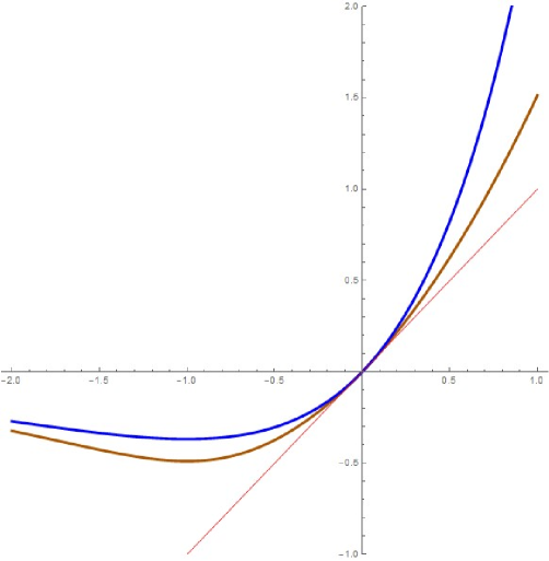
The half-iterate of b ( x ) = x exp ( x ) b(x)=x\exp(x)
b [ 1 / 2 ] ( x ) = { − h 6 ( − x ) if x < 0 , h 7 ( x ) if x > 0 b^{[1/2]}(x)=\left\{\begin{array}[c]{lll}-h_{6}(-x)&&\text{if }x<0,\\
h_{7}(x)&&\text{if }x>0\end{array}\right.
where
h 6 ( x ) = g 6 [ − 1 ] ( g 6 ( x ) + 1 2 ) , h 7 ( x ) = g 7 [ − 1 ] ( g 7 ( x ) − 1 2 ) \begin{array}[c]{ccc}h_{6}(x)=g_{6}^{[-1]}\left(g_{6}(x)+\dfrac{1}{2}\right),&&h_{7}(x)=g_{7}^{[-1]}\left(g_{7}(x)-\dfrac{1}{2}\right)\end{array}
and is plotted in Figure 2. For example,
b [ 1 / 2 ] ( − 3 2 ) \displaystyle b^{[1/2]}\left(-\frac{3}{2}\right) = − 0.42641662941763325151531183149592820162632882697793 \ \displaystyle=-0.42641662941763325151531183149592820162632882697793\backslash
43063735255284490601822588280606246428889441780123 … , \displaystyle\;\;\;\;\;\;\;\;\;\;43063735255284490601822588280606246428889441780123...,
b [ 1 / 2 ] ( − 1 ) \displaystyle b^{[1/2]}(-1) = − 0.48866481866503552878680514997833634260324371454204 \ \displaystyle=-0.48866481866503552878680514997833634260324371454204\backslash
60274529527835852337101053917173648041964826593958 … , \displaystyle\;\;\;\;\;\;\;\;\;\;\;60274529527835852337101053917173648041964826593958...,
b [ 1 / 2 ] ( − 1 2 ) \displaystyle b^{[1/2]}\left(-\frac{1}{2}\right) = − 0.37347989775777905190541972368443720513046069581332 \ \displaystyle=-0.37347989775777905190541972368443720513046069581332\backslash
86554406703025989395393199161956685435603156864847 … , \displaystyle\;\;\;\;\;\;\;\;\;\;86554406703025989395393199161956685435603156864847...,
b [ 1 / 2 ] ( 1 2 ) \displaystyle b^{[1/2]}\left(\frac{1}{2}\right) = 0.62602395130210673371845533179246340067357867185364 \ \displaystyle=0.62602395130210673371845533179246340067357867185364\backslash
52196041180904364827145223720139252799764700719890 … , \displaystyle\;\;\;\;\;\;\;52196041180904364827145223720139252799764700719890...,
b [ 1 / 2 ] ( 1 ) \displaystyle b^{[1/2]}(1) = 1.51342810850016187455237845958023613605233037133027 \ \displaystyle=1.51342810850016187455237845958023613605233037133027\backslash
52630412064404423776816220701637052381526519832852 … . \displaystyle\;\;\;\;\;\;\;52630412064404423776816220701637052381526519832852....
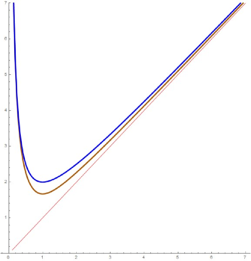
The half-iterate of d ( x ) = x + 1 / x d(x)=x+1/x
d [ 1 / 2 ] ( x ) = 1 g 8 [ − 1 ] ( g 8 ( x ) + 1 2 ) if x > 0 \begin{array}[c]{ccc}d^{[1/2]}(x)=\dfrac{1}{g_{8}^{[-1]}\left(g_{8}(x)+\dfrac{1}{2}\right)}&&\text{if }x>0\end{array}
and is plotted in Figure 3. For example,
d [ 1 / 2 ] ( 1 ) \displaystyle d^{[1/2]}(1) = 1.66827125814273410261365244553632620290300096260795 \ \displaystyle=1.66827125814273410261365244553632620290300096260795\backslash
45612116471428413629522821259531646886087189899654 … , \displaystyle\;\;\;\;\;\;\;\;45612116471428413629522821259531646886087189899654...,
d [ 1 / 2 ] ( 2 ) \displaystyle d^{[1/2]}(2) = 2.26769416081462195569866756632678174040589772138648 \ \displaystyle=2.26769416081462195569866756632678174040589772138648\backslash
06150199155621095539006524575786194598054301929223 … , \displaystyle\;\;\;\;\;\;\;\;06150199155621095539006524575786194598054301929223...,
d [ 1 / 2 ] ( 3 ) \displaystyle d^{[1/2]}(3) = 3.17156288055845899507943288783530404254252348671240 \ \displaystyle=3.17156288055845899507943288783530404254252348671240\backslash
85284281807613396012483190218839371168323598229023 … . \displaystyle\;\;\;\;\;\;\;\;85284281807613396012483190218839371168323598229023....
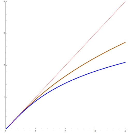
and d [ 1 / 2 ] ( 1 / x ) = d [ 1 / 2 ] ( x ) d^{[1/2]}(1/x)=d^{[1/2]}(x) arcsinh ( x ) \operatorname{arcsinh}(x)
arcsinh [ 1 / 2 ] ( x ) = g 9 [ − 1 ] ( g 9 ( x ) + 1 2 ) if x > 0 \begin{array}[c]{ccc}\operatorname{arcsinh}^{[1/2]}(x)=g_{9}^{[-1]}\left(g_{9}(x)+\dfrac{1}{2}\right)&&\text{if }x>0\end{array}
and is plotted in Figure 4. For example,
arcsinh [ 1 / 2 ] ( 1 ) \displaystyle\operatorname{arcsinh}^{[1/2]}\left(1\right) = 0.93556128335891826163999202492250530567588400325205 \ \displaystyle=0.93556128335891826163999202492250530567588400325205\backslash
31674271170225577872426642048379958915233196045102 … , \displaystyle\;\;\;\;\;\;\;\;31674271170225577872426642048379958915233196045102...,
arcsinh [ 1 / 2 ] ( 2 ) \displaystyle\operatorname{arcsinh}^{[1/2]}\left(2\right) = 1.66656170319583850033646701219094235941335779551333 \ \displaystyle=1.66656170319583850033646701219094235941335779551333\backslash
30718956939445848951705893403956452533778340335331 … . \displaystyle\;\;\;\;\;\;\;\;30718956939445848951705893403956452533778340335331....
Despite kindredness [3 ] of sin ( x ) \sin(x) arcsinh ( x ) \operatorname{arcsinh}(x) [6 ] surrounding sin [ 1 / 2 ] ( x ) \sin^{[1/2]}(x) arcsinh [ 1 / 2 ] ( x ) \operatorname{arcsinh}^{[1/2]}\left(x\right)
6 More delta conjectures
For θ 10 ( x ) = tanh ( x ) \theta_{10}(x)=\tanh(x)
g 10 ( 1 ) \displaystyle g_{10}(1) = 1.51079179586922388441504187983792771684880436991305 \ \displaystyle=1.51079179586922388441504187983792771684880436991305\backslash
75867903266412969163121334944455560618488719683881 … , \displaystyle\;\;\;\;\;\;\;75867903266412969163121334944455560618488719683881...,
g ~ 10 ( 1 ) \displaystyle\tilde{g}_{10}(1) = 1.44997202965299922711833991251827534636300580639368 \ \displaystyle=1.44997202965299922711833991251827534636300580639368\backslash
34571482244926753012114461573078658989846993713779 … \displaystyle\;\;\;\;\;\;\;34571482244926753012114461573078658989846993713779...
and evidently
δ 10 = g 10 ( x ) − g ~ 10 ( x ) = 3 20 ln ( 3 2 ) \delta_{10}=g_{10}\left(x\right)-\tilde{g}_{10}\left(x\right)=\frac{3}{20}\ln\left(\frac{3}{2}\right)
for all x > 0 x>0 θ 11 ( x ) = arctan ( x ) \theta_{11}(x)=\arctan(x)
g 11 ( 1 ) \displaystyle g_{11}(1) = 1.51105477063419552474681838379217653656603483006820 \ \displaystyle=1.51105477063419552474681838379217653656603483006820\backslash
45097278522747037923954184486447084322156741355942 … , \displaystyle\;\;\;\;\;\;\;45097278522747037923954184486447084322156741355942...,
g ~ 11 ( 1 ) \displaystyle\tilde{g}_{11}(1) = 1.57187453685042018204352035111182890705183339358757 \ \displaystyle=1.57187453685042018204352035111182890705183339358757\backslash
86393699544233254074961057857823985950798467326044 … \displaystyle\;\;\;\;\;\;\;86393699544233254074961057857823985950798467326044...
and evidently δ 11 = − δ 10 \delta_{11}=-\delta_{10}
For θ 12 ( x ) = x / 1 + x \theta_{12}(x)=x\left/\sqrt{1+x}\right.
g 12 ( 1 ) \displaystyle g_{12}(1) = 2.00378129463714162491795518942256698333039625079797 \ \displaystyle=2.00378129463714162491795518942256698333039625079797\backslash
55557419216169716071349148331180677424980811441121 … , \displaystyle\;\;\;\;\;\;\;55557419216169716071349148331180677424980811441121...,
g ~ 12 ( 1 ) \displaystyle\tilde{g}_{12}(1) = 2.35035488491711427962657125015165526736814631797810 \ \displaystyle=2.35035488491711427962657125015165526736814631797810\backslash
31828022616217183039458996804758706741615793534559 … \displaystyle\;\;\;\;\;\;\;31828022616217183039458996804758706741615793534559...
and evidently
δ 12 = g 12 ( x ) − g ~ 12 ( x ) = − 1 2 ln ( 2 ) = 1 2 ln ( 1 2 ) \delta_{12}=g_{12}\left(x\right)-\tilde{g}_{12}\left(x\right)=-\frac{1}{2}\ln(2)=\frac{1}{2}\ln\left(\frac{1}{2}\right)
for all x > 0 x>0 g ~ 12 ( 1 ) \tilde{g}_{12}\left(1\right) [12 ] . More generally, for arbitrary p > 0 p>0 θ ( x ) = x / ( 1 + x ) p \theta(x)=x/(1+x)^{p}
δ ( p ) = 1 − p 2 p ln ( p ) . \delta(p)=\frac{1-p}{2p}\ln(p).
Generalizing θ 8 ( x ) = x / ( 1 + x 2 ) \theta_{8}(x)=x/(1+x^{2}) x / ( 1 + x q ) x/(1+x^{q}) q > 0 q>0
Figure 1: Abel solutions for x exp ( x ) x\exp(x) x exp ( x ) x\exp(x) Figure 2: Half-iterate of x exp ( x ) x\exp(x) x exp ( x ) x\exp(x) Figure 3: Half-iterate of x + 1 / x x+1/x x + 1 / x x+1/x Figure 4: Half-iterate of arcsinh ( x ) \operatorname{arcsinh}(x) arcsinh ( x ) \operatorname{arcsinh}(x)
7 Acknowledgements
I am grateful to Daniel Lichtblau at Wolfram Research for kindly answering my
questions, e.g., about generalizing my original Mathematica code for ML to
arbitrary k k [9 ] assisted me in more ways than he
can imagine. The creators of Mathematica earn my gratitude every day: this
paper could not have otherwise been written. An interactive computational
notebook about ML is available [13 ] which might be useful to
interested readers; an analog for EJ is forthcoming.
References
[1]
F. Bencherif and G. Robin, Sur l’itéré de sin ( x ) \sin(x) Publ. Inst. Math. (Beograd) 56(70) (1994) 41–53; MR1349068; http://eudml.org/doc/256122.
[2]
S. Mavecha and V. Laohakosol, Asymptotic expansions of
iterates of some classical functions, Appl. Math. E-Notes 13 (2013)
77–91; MR3121616; http://www.emis.de/journals/AMEN/2013/2013.htm.
[3]
S. R. Finch, What do sin ( x ) \sin(x) arcsinh ( x ) \operatorname{arcsinh}(x)
[4]
J. Écalle, Théorie itérative: introduction à
la théorie des invariants holomorphes, J. Math. Pures Appl. 54
(1975) 183–258; MR0499882.
[5]
M. Kuczma, B. Choczewski and R. Ger, Iterative
Functional Equations , Cambridge Univ. Press, 1990, pp. 346–347, 351–352; MR1067720.
[6]
S. R. Finch, Half-iterates of x ( 1 + x ) x(1+x) sin ( x ) \sin(x) exp ( x / e ) \exp(x/e)
[7]
D. Kouznetsov, Super sin, Far East J. Math. Sci. 85
(2014) 219–238; http://mizugadro.mydns.jp/PAPERS/.
[8]
H. S. Wilf, generatingfunctionology , 2nd {}^{\text{nd}}
[9]
W. Jagy, Half iterate of x 2 + c x^{2}+c
[10]
M. Aschenbrenner and W. Bergweiler, Julia’s equation and
differential transcendence. Illinois J. Math. 59 (2015) 277–294;
arXiv:1307.6381; MR3499512.
[11]
T. Curtright and C. Zachos, Evolution profiles and
functional equations, J. Phys. A 42 (2009) 485208; arXiv:0909.2424; MR2562978.
[12]
S. R. Finch, Popa’s “Recurrent
sequences” and reciprocity, arXiv:2412.11806.
[13]
S. R. Finch, Iterational asymptotics of sine and cosine,
Steven Finch
MIT Sloan School of Management
Cambridge, MA, USA
steven_finch_math@outlook.com