Robust Transceiver Design for RIS Enhanced Dual-Functional Radar-Communication with Movable Antenna

Abstract

Movable antennas (MAs) have demonstrated significant potential in enhancing the performance of dual-functional radar-communication (DFRC) systems. In this paper, we explore an MA-aided DFRC system that utilizes a reconfigurable intelligent surface (RIS) to enhance signal coverage for communications in dead zones. To enhance the radar sensing performance in practical DFRC environments, we propose a unified robust transceiver design framework aimed at maximizing the minimum radar signal-to-interference-plus-noise ratio (SINR) in a cluttered environment. Our approach jointly optimizes transmit beamforming, receive filtering, antenna placement, and RIS reflecting coefficients under imperfect channel state information (CSI) for both sensing and communication channels. To deal with the channel uncertainty-constrained issue, we leverage the convex hull method to transform the primal problem into a more tractable form. We then introduce a two-layer block coordinate descent (BCD) algorithm, incorporating fractional programming (FP), successive convex approximation (SCA), S-Lemma, and penalty techniques to reformulate it into a series of semidefinite program (SDP) subproblems that can be efficiently solved. We provide a comprehensive analysis of the convergence and computational complexity for the proposed design framework. Simulation results demonstrate the robustness of the proposed method, and show that the MA-based design framework can significantly enhance the radar SINR performance while achieving an effective balance between the radar and communication performance.

I Introdution

As the landscape of wireless communications continues to evolve, the anticipation surrounding the advent of sixth generation (6G) networks is steadily growing[2, 3]. According to the International Telecommunication Union Telecommunication Standardization Sector (ITUT), 6G is expected to support various usage scenarios including immersive communication, hyper reliable and low-latency communication (HRLLC), massive communication, artificial intelligence (AI) and communication, ubiquitous connectivity, and integrated sensing and communication (ISAC)[4]. These usage scenarios form the vision of International Mobile Telecommunication (IMT)-2030, and necessitate a paradigm shift in current fifth generation (5G) wireless networks [5]. In particular, dual-functional radar-communications (DFRC), which integrates sensing and communication functions into a single platform, has been envisioned as a key transformative technology for the upcoming generation [6]. DFRC systems share spectrum resources, hardware facilities, and signal-processing modules, resulting in significantly increased spectrum efficiency [7]. Thanks to these advantages, DFRC has shown great potential in various wireless systems, such as orthogonal time frequency space modulation (OTFS)[8], non-orthogonal multiple access (NOMA)[9], and unmanned aerial vehicle (UAV)[10].

Despite extensive research on DFRC [8, 9, 10], conventional multiple-input multiple-output (MIMO) systems with fixed-position antennas (FPAs) still present significant challenges in terms of power consumption and interference mitigation [11]. Specifically, FPA array configurations limit the full exploration of diversity and spatial multiplexing gains of wireless channels, as they do not fully utilize channel variations across continuous spatial fields. Furthermore, the fixed geometric configurations of antenna arrays can lead to array gain loss during the radar beamforming tasks. Therefore, beyond developing advanced optimization algorithms and intelligent resource management strategies, introducing new revolutionary technologies such as reconfigurable antennas is also critically important.

Recently, movable antennas (MAs), also named as fluid antennas[12], have been proposed as an innovative solution to overcome the fundamental limitations of conventional FPA-based systems [13]. MAs enable flexible adjustment of antenna element positions at the transceiver within a local movement region. Specifically, in the MA-assisted systems, each antenna element is connected to a radio frequency (RF) chain via flexible cables to support active movement, thereby reconstructing channel conditions to boost both the communication and radar performance [14]. Channel modeling and performance analysis were initially explored in [15], where the authors established a field-response channel model under the far-field conditions. Based on the results in [15], recent studies have shown that the dual-task performance can be significantly boosted by properly adjusting the positions of MAs within a designated area [16, 17, 18, 19, 20, 21]. For instance, in [16], the authors proposed a three-stage search-based projected gradient ascent (GA) method to enhance the DFRC performance. The authors in [17] investigated a deep reinforcement learning method for the optimization on joint port selection and precoder for the MA-enhanced DFRC systems. In addition, the MA-based cooperative DFRC network was investigated in [20, 21]. With operations in higher frequency bands, the near-field sensing and communication channels regarding MA positions were characterized by using the spherical wave model in [22]. Although these studies have demonstrated the superiority of MA over FPA, the susceptibility of radio signals to blockage and attenuation events has not yet been fully investigated, which inevitably limits the full potential of the MA technique.

Reconfigurable intelligent surface (RIS) is considered as a promising technology to address the aforementioned challenges[23]. An RIS is a planar array made up of many passive reflecting elements with controllable phase shifts[24]. Consequently, the RIS can not only reconfigure the wireless channels but also provide the line-of-sight (LoS) links for both communication and sensing tasks in dead zones [25]. Recent studies have explored the integration of RIS into the MA-assisted DFRC systems[26, 27]. Specifically, an MA-assisted secure transmission scheme for the RIS-DFRC systems was investigated in [26]. The authors in [27] focused on maximizing the minimum beampattern gain for the MA-based RIS-DFRC systems. Nevertheless, these models are relatively simple, considering only clutter-free environments [26] or focusing on designing the transmitter [27], which inevitably leads to the degraded communication and sensing performance. Furthermore, these works typically assume perfect knowledge of the target locations and communication channels, and the role of MAs in robust transmission has not been thoroughly unveiled. As a result, to fully unlock the potential of the MA technique, a unified MA-based transceiver design framework to tackle these issues is greatly desirable.

In this paper, we investigate the robust transceiver design for RIS-enhanced DFRC systems with movable antennas. Specifically, we consider a monostatic DFRC system where a dual-functional base station (BS) equipped with 2D transceiver MA arrays serves multiple users and detects a point-like target in a cluttered environment. An RIS is deployed to create virtual LoS links for the communications in dead zones. In particular, our contributions can be summarized as follows.

• To enhance the radar sensing performance, a unified robust transceiver design framework is developed to maximize the radar SINR by jointly optimizing the positions of MAs, the transmitting beamforming, the receiving filter, and the RIS reflecting coefficients under imperfect channel state information (CSI) for both sensing and communication channels.

• We formulate an optimization problem to maximize the minimum radar SINR with regard to worst-case locations within the uncertain interval subject to the quality of service (QoS) constraints under the bounded communication channel error model. To deal with the channel uncertainty-constrained problem, we leverage the convex hull method to transform the primal problem into a more tractable form. We develop a two-layer block coordinate descent-based algorithm, combined with fractional programming (FP), successive convex approximation (SCA), S-Lemma, and penalty techniques to convert it into a sequence of semidefinite program (SDP) subproblems that can be efficiently solved.

• To evaluate the corresponding robust designs, we revise the algorithm framework for the perfect CSI case to serve as a performance upper bound. We further provide a comprehensive analysis of the convergence and computational complexity for the proposed algorithms in both cases with perfect and imperfect CSI.

• Simulation results demonstrate that the proposed MA-based transceiver design framework exhibits remarkable robustness across various levels of channel uncertainty, and can significantly improve the minimum radar SINR while achieving a satisfactory trade-off between the radar and communication performance.

Notations: Boldface lower-case and upper-case letters indicate column vectors and matrices, respectively. $(\cdot)^{*}$, $(\cdot)^{T}$, $(\cdot)^{H}$, and $(\cdot)^{-1}$ denote the conjugate, transpose, transpose-conjugate, and inverse operations, respectively. $\mathbb{C}$ and $\mathbb{R}$ denote the sets of complex numbers and real numbers, respectively. $|a|$, $\|\bm{a}\|$, and $\|\bm{A}\|_{F}$ are the magnitude of a scalar $a$, the norm of a vector $\bm{a}$, and the Frobenius norm of a matrix $\bm{A}$, respectively. $\mathbb{E}\{\cdot\}$ represents statistical expectation. $\text{Tr}\{\bm{A}\}$ takes the trace of the matrix $\bm{A}$. $\Re\{\cdot\}$ and $\Im\{\cdot\}$ denote the real and imaginary parts of a complex number, respectively. $\angle a$ is the angle of complex-valued $a$. $\bm{I}_{M}$ indicates an $M\times M$ identity matrix.

II System Model

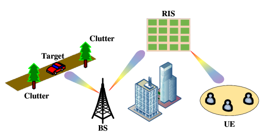
Figure 1: System model.

We consider a DFRC system as depicted in Fig. 1, where the dual-functional BS equipped with a planar array consisting of $N$ transmitting/receiving movable antennas serves $K$ single-antenna users while detecting a point-like target in the presence of $Q$ clutters. It is assumed that the direct links from the BS to the users are not available due to blockages, thus an $M$-element RIS is deployed to create virtual LoS links. The 2D moving regions for the transceiver antennas are respectively denoted by $\mathcal{C}_{t}$ and $\mathcal{C}_{r}$, both consisting of a square region of size $A\times A$. Moreover, the positions of the $n$-th transmitting and receiving antenna MAs are denoted by $\bm{t}_{n}=[x_{n}^{t},y_{n}^{t}]^{T}$ and $\bm{r}_{n}=[x_{n}^{r},y_{n}^{r}]^{T}$, with the reference points for the regions $\mathcal{C}_{t}$ and $\mathcal{C}_{r}$ represented by $\bm{o}^{t}=\bm{o}^{r}=[0,0]^{T}$, respectively.

II-A Communication Model

Let $\bm{w}_{k}$ represent the beamforming vector for the user $k$, the signal $\bm{x}\in\mathbb{C}^{N\times 1}$ transmitted by the BS can be written as

$$\bm{x}=\bm{Ws}=\sum_{k=1}^{K}\bm{w}_{k}s_{k},$$ (1)

where $\bm{s}=[s_{1},\dots,s_{K}]^{T}\in\mathbb{C}^{K\times 1}$ with $\mathbb{E}[\bm{s}\bm{s}^{H}]=\bm{I}_{K}$ represents the data symbols for all the users . Given that the signal propogation distance is significantly larger than the size of the moving regions, the far-field response can be applied for channel modeling [28]. Specifically, the angle-of-arrival (AoA), angle-of-departure (AoD), and amplitude of the complex coefficient for each link remain constant despite the movement of the MAs. Note that we adopt the geometric model for the communication channels, thus the number of transmission paths at different nodes are the same, denoted by $L$[15]. The elevation and azimuth angles of the $j$-th transmission path at the BS and RIS are given by $\psi^{e}_{j}\in[0,\pi],\psi^{a}_{j}\in[0,\pi]$ and $\phi^{e}_{j}\in[0,\pi],\phi^{a}_{j}\in[0,\pi]$, respectively. Then, for the $j$-th transmission path, the signal propagation difference between the position of the $n$-th transmitting MA $\bm{t}_{n}$ and the reference point $\bm{o}^{t}$ is given by

$$\rho(\bm{t}_{n},\psi^{e}_{j},\psi_{j}^{a})=x^{t}_{n}\sin\psi^{e}_{j}\cos\psi^{a}_{j}+y^{t}_{n}\cos\psi^{e}_{j}.$$ (2)

Then, the field response vector (FRV) at $\bm{t}_{n}$ can be given by

$$\bm{g}(\bm{t}_{n})=\left[e^{\jmath\frac{2\pi}{\lambda}\rho(\bm{t}_{n},\psi^{e}_{1},\psi_{1}^{a})},\dots,e^{\jmath\frac{2\pi}{\lambda}\rho(\bm{t}_{n},\psi^{e}_{L},\psi_{L}^{a})}\right]^{T}\in\mathbb{C}^{L\times 1},$$ (3)

where $\lambda$ is the carrier wavelength. Therefore, the field response matrix (FRM) of the BS-RIS link for all $N$ transmitting MAs is given by

$$\bm{G}(\tilde{\bm{t}})\triangleq\left[\bm{g}(\bm{t}_{1}),\bm{g}(\bm{t}_{2}),\dots,\bm{g}(\bm{t}_{N})\right]\in\mathbb{C}^{L\times N},$$ (4)

where $\tilde{\bm{t}}\triangleq\left[\bm{t}_{1}^{T},\bm{t}_{2}^{T},\dots,\bm{t}_{N}^{T}\right]^{T}\in\mathbb{R}^{2N\times 1}$. Similarly, the FRV at the $m$-th RIS reflecting element can be derived as

$$\bm{f}(\bm{s}_{m})=\left[e^{\jmath\frac{2\pi}{\lambda}\rho(\bm{s}_{m},\phi_{1}^{e},\phi_{1}^{a})},\dots,e^{\jmath\frac{2\pi}{\lambda}\rho(\bm{s}_{m},\phi_{L}^{e},\phi_{L}^{a})}\right]^{T}\in\mathbb{C}^{L\times 1},$$ (5)

where $\bm{s}_{m}=[x_{m}^{s},y_{m}^{s}]^{T}$ is the coordinate of the $m$-th element, and $\rho(\bm{s}_{m},\phi_{j}^{e},\phi_{j}^{a})$ denotes the propagation distance difference for the $j$-th path between the position $\bm{s}_{m}$ and origin of the RIS, $\bm{o}^{s}=[0,0]^{T}$. Then, the FRM at the RIS can be given by

$$\bm{F}({\tilde{\bm{s}}})\triangleq\left[\bm{f}(\bm{s}_{1}),\bm{f}(\bm{s}_{2}),\dots,\bm{f}(\bm{s}_{M})\right]^{T}\in\mathbb{C}^{L\times M}.$$ (6)

Let $\bm{\Sigma}=\mathrm{diag}\{\sigma_{1,1},\sigma_{2,2},\dots,\sigma_{L,L}\}\in\mathbb{C}^{L\times L}$ denote the path response matrix (PRM) of the BS-RIS link, the channel matrix can be expessed as

$$\bm{H}(\tilde{\bm{t}})=\bm{F}({\tilde{\bm{s}}})^{H}\bm{\Sigma}\bm{G}(\tilde{\bm{t}})\in\mathbb{C}^{M\times N}.$$ (7)

The channel $\bm{h}_{k}\in\mathbb{C}^{M\times 1}$ between the RIS and the $k$-th user can be derived in a similar fashion as (7) and is thus omitted for brevity. The received signal of the $k$-th user is given by

$$y_{k}=\underbrace{\bm{h}_{k}^{H}\bm{V}\bm{H}(\tilde{\bm{t}})\bm{w}_{k}s_{k}}_{\text{desired signal}}+\underbrace{\sum_{j=1,j\neq k}^{K}\bm{h}_{k}^{H}\bm{V}\bm{H}(\tilde{\bm{t}})\bm{w}_{j}s_{j}}_{\text{inter-user interference}}+n_{k},$$ (8)

where $\bm{V}=\mathrm{diag}\{[v_{1},\dots,v_{M}]^{T}\}\in\mathbb{C}^{M\times M}$ with $v_{m}=e^{\jmath\theta_{m}}$ being the reflection coefficient matrix, and $n_{k}\sim\mathcal{CN}(0,\sigma_{k}^{2})$ is the additive white Gaussian noise (AWGN). Then, the SINR of the $k$-th user is given by

$$\Gamma_{k}(\bm{W},\bm{V},\tilde{\bm{t}})=\frac{|\bm{h}_{k}^{H}\bm{V}\bm{H}(\tilde{\bm{t}})\bm{w}_{k}|^{2}}{\sum_{j=1,j\neq k}^{K}|\bm{h}_{k}^{H}\bm{V}\bm{H}(\tilde{\bm{t}})\bm{w}_{j}|^{2}+\sigma_{k}^{2}}.$$ (9)

II-B Radar Model

We adopt the LoS channel model for the sensing channels between the BS and the target/clutters. Let $\varphi_{0}^{e}$ and $\varphi_{0}^{a}$ denote the elevation and azimuth angle between the target and the BS, the receiving and transmitting steering vectors can be given by $\mathbf{a}_{0}^{r}(\varphi_{0}^{e},\varphi_{0}^{a},\tilde{\bm{r}})=[e^{\jmath\frac{2\pi}{\lambda}\rho(\bm{r}_{1},\varphi_{0}^{e},\varphi_{0}^{a})},\dots,e^{\jmath\frac{2\pi}{\lambda}\rho(\bm{r}_{N},\varphi_{0}^{e},\varphi_{0}^{a})}]^{T}$ and $\mathbf{a}_{0}^{t}(\varphi_{0}^{e},\varphi_{0}^{a},\tilde{\bm{t}})=[e^{\jmath\frac{2\pi}{\lambda}\rho(\bm{t}_{1},\varphi_{0}^{e},\varphi_{0}^{a})},\dots,e^{\jmath\frac{2\pi}{\lambda}\rho(\bm{t}_{N},\varphi_{0}^{e},\varphi_{0}^{a})}]^{T}$, respectively. Let $\bm{A}_{0}(\tilde{\bm{r}},\tilde{\bm{t}})=\mathbf{a}_{0}^{r}(\varphi_{0}^{e},\varphi_{0}^{a},\tilde{\bm{r}})\mathbf{a}_{0}^{t}(\varphi_{0}^{e},\varphi_{0}^{a},\tilde{\bm{t}})^{H}$ denote the response matrix for the target, and the received echo signal can be given by

$$y_{r}=\alpha_{0}\bm{u}^{H}\bm{A}_{0}(\tilde{\bm{r}},\tilde{\bm{t}})\bm{x}+\bm{u}^{H}\bm{c}+\bm{u}^{H}\bm{n}_{r},$$ (10)

where $\bm{c}=\sum_{q=1}^{Q}\alpha_{q}\bm{A}_{q}(\tilde{\bm{r}},\tilde{\bm{t}})\bm{x}$, $\bm{A}_{q}(\tilde{\bm{r}},\tilde{\bm{t}})=\mathbf{a}_{q}^{r}(\varphi_{q}^{e},\varphi_{q}^{a},\tilde{\bm{r}})\mathbf{a}_{q}^{t}(\varphi_{q}^{e},\varphi_{q}^{a},\tilde{\bm{t}})^{H}$ denotes the response matrix for the $q$-th clutter, and $\bm{u}\in\mathbb{C}^{N\times 1}$ is the receiving filter. Here, $\alpha_{0}$ and $\alpha_{q}$ are the complex coefficients including the radar cross section (RCS) and the cascaded complex gain of the target and $q$-th clutter, with $\mathbb{E}\{|\alpha_{0}|^{2}\}=\zeta_{0}^{2}~\text{and}~\mathbb{E}\{|\alpha_{q}|^{2}\}=\zeta_{q}^{2}$, respectively. Besides, $\bm{n}_{r}\sim\mathcal{CN}(0,\sigma_{r}^{2}\bm{I}_{N})$ is the AWGN at the BS. To maximize the radar SINR, the optimal solution for the filter $\bm{u}^{\star}$ can be obtained by solving the minimum variance distortionless response (MVDR) problem [29], i.e.,

$$\bm{u}^{\star}=\beta\left(\bm{c}\bm{c}^{H}+\bm{n}_{r}\bm{n}_{r}^{H}\right)^{-1}\bm{A}_{0}(\tilde{\bm{r}},\tilde{\bm{t}})\bm{x},$$ (11)

where $\beta$ is an auxiliary constant. Then, the average radar SINR can be derived as [17], i.e.,

$$\Gamma(\bm{W} ,\tilde{\bm{r}},\tilde{\bm{t}})$$

$$\mathop{=}\limits^{\left({a}\right)}~{\mathbb{E}}\left[|\alpha_{0}|^{2}\bm{x}^{H}\bm{A}_{0}(\tilde{\bm{r}},\tilde{\bm{t}})^{H}(\bm{c}\bm{c}^{H}+\bm{n}_{r}\bm{n}_{r}^{H})^{-1}\bm{A}_{0}(\tilde{\bm{r}},\tilde{\bm{t}})\bm{x}\right]$$

$$\mathop{\geq}\limits^{\left({b}\right)}~{\mathrm{tr}}\left({\bm{\Phi}}\bm{W}\bm{W}^{H}\right)\triangleq\Gamma_{r}(\bm{W},\tilde{\bm{r}},\tilde{\bm{t}}),$$ (12)

where ${\bm{\Phi}}=\zeta_{0}^{2}\bm{A}_{0}(\tilde{\bm{r}},\tilde{\bm{t}})^{H}(\bm{\Xi}+\sigma_{r}^{2}\bm{I}_{N})^{-1}\bm{A}_{0}(\tilde{\bm{r}},\tilde{\bm{t}}),$ and $\bm{\Xi}=\sum_{q=1}^{Q}\zeta_{q}^{2}\bm{A}_{q}(\tilde{\bm{r}},\tilde{\bm{t}})\bm{W}\bm{W}^{H}\bm{A}_{q}(\tilde{\bm{r}},\tilde{\bm{t}})^{H}$. Note that the procedure (a) is due to the optimal receiving filter $\bm{u}^{\star}$ in (11), and the procedure (b) holds due to Jesen’s inequality, $\mathbb{E}[\bm{xx}^{H}]=\bm{W}\bm{W}^{H}$, $\mathbb{E}[\bm{cc}^{H}]=\bm{\Xi}$, and $\mathbb{E}\{|\alpha_{0}|^{2}\}=\zeta_{0}^{2}$.

II-C Channel Uncertainty Model

In practical DFRC scenarios, acquiring perfect knowledge for both communcation and sensing channels is chanllenging. Specifically, for the communication part, although various channel estimation methods have been developed for the MA and RIS-aided communications [23, 13], the perfect CSI for the reflecting links is difficult to obtain due to the limited signal processing capabilities of passive RIS elements, and fast change of user locations. To characterize this effect, we exploit the bounded CSI error model to quantify the CSI uncertainty of the RIS-user channels [30], i.e.,

$$\bm{h}_{k}=\hat{\bm{h}}_{k}+\Delta\bm{h}_{k},||\Delta\bm{h}_{k}||_{2}\leq\varepsilon_{k},$$ (13)

where $\hat{\bm{h}}_{k}$ is the estimated channel vector, and $\varepsilon_{k}$ is the radius of the uncertainty region for the $k$-th user known by the BS.

For the sensing part, we assume that the target location is not perfectly known to the BS due to its movement and random fluctuation [29]. That is, the target is located in an uncertain angular interval, such that

$$\Psi_{e}=\big{[}\vartheta_{e}-\frac{1}{2}\Delta\vartheta_{e},\vartheta_{e}+\frac{1}{2}\Delta\vartheta_{e}\big{]},$$ (14a)

$$\Psi_{a}=\big{[}\vartheta_{a}-\frac{1}{2}\Delta\vartheta_{a},\vartheta_{a}+\frac{1}{2}\Delta\vartheta_{a}\big{]},$$ (14b)

where $\Delta\vartheta_{e}$ and $\Delta\vartheta_{a}$ denote the elevation and azimuth error range, respectively.

II-D Problem Formulation

Based on the above performance metrics, we focus on the robust transceiver design under both imperfect communication and sensing channels. Specifically, we aim to maximize the minimum radar SINR performance with regard to worst-case locations within the uncertain interval $\Psi_{e}$ and $\Psi_{a}$ subject to the given QoS constraints under the bounded CSI error model. This is achieved by jointly designing the transmitting beamforming vectors, positions of transceiver antennas, and RIS reflecting elements. In particular, the optimization problem can be formulated as

$$\underset{\bm{W},\bm{V},\tilde{\bm{t}},\tilde{\bm{r}}}{\max}~~\underset{\begin{subarray}{c}\varphi_{0}^{e}\in\Psi_{e}\\ \varphi_{0}^{a}\in\Psi_{a}\end{subarray}}{\min}~~\Gamma_{r}(\bm{W},\tilde{\bm{r}},\tilde{\bm{t}})$$ (15a)

$$\,\text{s.t.}~\Gamma_{k}(\bm{W},\bm{V},\tilde{\bm{t}})\geq\gamma_{k},||\Delta\bm{h}_{k}||_{2}\leq\varepsilon_{k},\forall k,$$ (15b)

$$\hphantom{s.t.~}||\bm{t}_{n}-\bm{t}_{n^{\prime}}||_{2}^{2}\geq D^{2},||\bm{r}_{n}-\bm{r}_{n^{\prime}}||_{2}^{2}\geq D^{2},\forall n\neq n^{\prime},$$ (15c)

$$\hphantom{s.t.~}\bm{t}_{n}\in\mathcal{C}_{t},\bm{r}_{n}\in\mathcal{C}_{r},\forall n,$$ (15d)

$$\hphantom{s.t.~}\sum_{k=1}^{K}\bm{w}_{k}^{H}\bm{w}_{k}\leq P_{t},$$ (15e)

$$\hphantom{s.t.~}|{v}_{m}|^{2}=1,\forall m,$$ (15f)

where the constraints in (15b) ensure that the SINR at the $k$-th user is no less than the predefined threshold $\gamma_{k}$, $D$ represents the minimum distance between the MAs to prevent coupling effects, $P_{t}$ is the maximum transmission power, and (15f) are the unit-modulus constraints on RIS. It is challenging to solve the above problem due to the non-convexity of (15b), (15c), (15d), (15e), as well as the coupling between optimization variables. The angle uncertainty and CSI errors further increase the difficulty of solving the problem in (15).

III Two-layer BCD Algorithm

Note that the inaccurate location region of the sensing target is a continuous area, which makes the problem in (15) non-convex and mathematically intractable. The random communication CSI errors further increase the difficulty. To deal with these issues, we leverage the convex hull technique to transform the original problem in (15) into a more tractable form, and develop a two-layer block coordinate descent (BCD) algorithm to solve it, the details of which are elaborated as follows.

III-A Problem Transformation

Based on the concept of convex hull, any channel matrix in an uncertainty set can be represented as a weighted combination of discrete samples[31]. Following this idea, we first uniformly discretize the continuous region, with the number of sampling points denoted by $P_{s}$. Let $(\varphi_{p}^{e},\varphi_{p}^{a})$ denote the $p$-th possible location, and we construct a convex hull based on the weighted sum of $P_{s}$ steering matrix samples, i.e.,

$$\Upsilon=\Big{\{}\sum_{p=1}^{P_{s}}\mu_{p}\bm{A}_{p}(\tilde{\bm{r}},\tilde{\bm{t}})|\sum_{p=1}^{P_{s}}\mu_{p}=1,\mu_{p}\geq 0\Big{\}},$$ (16)

where $\bm{A}_{p}(\tilde{\bm{r}},\tilde{\bm{t}})=\mathbf{a}_{p}^{r}(\varphi_{p}^{e},\varphi_{p}^{a},\tilde{\bm{r}})\mathbf{a}_{p}^{t}(\varphi_{p}^{e},\varphi_{p}^{a},\tilde{\bm{t}})^{H}$, and $\bm{\mu}=[\mu_{1},\dots,\mu_{P_{s}}]^{T}\in\mathbb{C}^{P_{s}\times 1}$ is the weighted coefficient vector. Let ${\tilde{\bm{\Phi}}}=\zeta_{0}^{2}\sum_{p=1}^{P_{s}}\mu_{p}\bm{A}_{p}(\tilde{\bm{r}},\tilde{\bm{t}})^{H}(\bm{\Xi}+\sigma_{r}^{2}\bm{I}_{N})^{-1}\sum_{p=1}^{P_{s}}\mu_{p}\bm{A}_{p}(\tilde{\bm{r}},\tilde{\bm{t}})$, and we construct a surrogate function for (15a) to facilitate the algorithm development, i.e.,

$$\tilde{\Gamma}_{r}(\bm{W},\tilde{\bm{r}},\tilde{\bm{t}},\bm{\mu})={\mathrm{tr}}\left({\tilde{\bm{\Phi}}}\bm{W}\bm{W}^{H}\right).$$ (17)

We then demonstrate the relationship between (15a) and (17), i.e.,

$$\underset{\bm{W},\bm{V},\tilde{\bm{t}},\tilde{\bm{r}}}{\max}~\underset{\begin{subarray}{c}\varphi_{0}^{e}\in\Psi_{e}\\ \varphi_{0}^{a}\in\Psi_{a}\end{subarray}}{\min}~\Gamma_{r}(\bm{W},\tilde{\bm{r}},\tilde{\bm{t}})\geq\underset{\bm{W},\bm{V},\tilde{\bm{t}},\tilde{\bm{r}}}{\max}\underset{\bm{\mu}}{\min}~\tilde{\Gamma}_{r}(\bm{W},\tilde{\bm{r}},\tilde{\bm{t}},\bm{\mu})$$

$$=\underset{\bm{\mu}}{\min}\underset{\bm{W},\bm{V},\tilde{\bm{t}},\tilde{\bm{r}}}{\max}~\tilde{\Gamma}_{r}(\bm{W},\tilde{\bm{r}},\tilde{\bm{t}},\bm{\mu}).$$ (18)

Proof: Please refer to the Appendix A in [32]. $\Box$

It can be observed that the surrogate objective function in (17) is highly intractable due to the coupling of the optimization variables. To tackle this challenge, we decouple the revised problem into the following two parts, i.e.,

$$(\text{P1}):~~\max\limits_{\bm{W},\bm{V},\tilde{\bm{t}},\tilde{\bm{r}}}\tilde{\Gamma}_{r}(\bm{W},\tilde{\bm{r}},\tilde{\bm{t}})$$

$$\qquad\quad\,\text{~s.t}.~\text{(\ref{robust1_Com}),~(\ref{robust1_MA1}),~(\ref{robust1_MA2}),~(\ref{robust1_Pt}),~(\ref{robust1_RIS})},$$ (19)

$$(\text{P2}):~~\min\limits_{\bm{\mu}}~\tilde{\Gamma}_{r}(\bm{\mu})$$

$$\qquad\quad\,~\text{s.t.~}\sum_{p=1}^{P_{s}}\mu_{p}=1,~\mu_{p}>=0.$$ (20)

Then, we propose a two-layer BCD-based algorithm to solve the problems (P1) and (P2) in an iterative manner until convergence, the details of which are given as follows.

III-B Optimization on (P1)

To facilitate the algorithm development, we first employ the fractional programming method in  [33] to equivalently convert the objective function in (19) into a more tractable form as

$$\bar{\Gamma} {}_{r}(\bm{W},\tilde{\bm{r}},\tilde{\bm{t}},\bm{\Lambda})=$$

$$\zeta_{0}^{2}\mathrm{tr}\left(2\Re\{\bm{W}^{H}\sum_{p=1}^{P_{s}}\mu_{p}\bm{A}_{p}(\tilde{\bm{r}},\tilde{\bm{t}})^{H}\bm{\Lambda}\}-\bm{\Lambda}^{H}(\bm{\Xi}+\sigma_{r}^{2}\bm{I}_{N})\bm{\Lambda}\right),$$ (21)

where $\bm{\Lambda}\in\mathbb{C}^{N\times K}$ is an auxiliary variable. Based on the reformulated objective function in (III-B), we propose a BCD-based algorithm by incorporating SCA, S-Lemma, and penalty techiques to solve the problem in (19), the procedures of which are given as follows.

III-B1 Updating Auxiliary Variable

Note that determining the optimal value of $\bm{\Lambda}$ is an unconstrained optimization problem, and the optimal solution $\bm{\Lambda}^{\star}$ can be directly given by

$$\bm{\Lambda}^{\star}=\left(\bm{\Xi}+\sigma_{r}^{2}\bm{I}_{N}\right)^{-1}\sum_{p=1}^{P_{s}}\mu_{p}\bm{A}_{p}(\tilde{\bm{r}},\tilde{\bm{t}})\bm{W}.$$ (22)

III-B2 Updating Transmit Beamforming

With $\tilde{\bm{r}},\tilde{\bm{t}},\bm{\Lambda}$ and $\bm{V}$ being fixed, the problem in (19) can be recast as

$$\underset{\bm{W}}{\max}\quad\bar{\Gamma}_{r}(\bm{W})$$ (23a)

$$\,\text{s.t.}~\Gamma_{k}(\bm{W})\geq\gamma_{k},||\Delta\bm{h}_{k}||_{2}\leq\varepsilon_{k},\forall k,$$ (23b)

$$\hphantom{s.t.~}\sum_{k=1}^{K}\bm{w}_{k}^{H}\bm{w}_{k}\leq P_{t}.$$ (23c)

It is observed that the non-convexity of the above problem lies in the constraints in (23b) over the CSI uncertainty regions. To deal with this issue, we rewrite the constraints in (23b) as

$$|\bm{h}_{k}^{H}\bm{V}\bm{H}(\tilde{\bm{t}})\bm{w}_{k}|^{2}\geq z_{k}\gamma_{k},||\Delta\bm{h}_{k}||_{2}\leq\varepsilon_{k},\forall k,$$ (24a)

$$||\bm{h}_{k}^{H}\bm{V}\bm{H}(\tilde{\bm{t}})\bm{W}_{-k}||_{2}^{2}+\sigma_{k}^{2}\leq z_{k},||\Delta\bm{h}_{k}||_{2}\leq\varepsilon_{k},\forall k,$$ (24b)

where $\bm{W}_{-k}=[\bm{w}_{1},\dots,\bm{w}_{k-1},\bm{w}_{k+1},\dots,\bm{w}_{K}]\in\mathbb{C}^{N\times(K-1)},$ and $\bm{z}=[z_{1},\dots,z_{K}]^{T}\in\mathbb{C}^{K\times 1}$ are the auxiliary variables. The equivalence between (24) and (23b) can be verified by contradiction. We first handle the non-convex quadratic inequalities in (24a). Specifically, the left-hand-side (LHS) of (24a) is approximated with its lower bound, as shown below.

Lemma 1: Let $\bm{w}_{k}^{(l)}$ and $\bm{V}^{(l)}$ be the optimal solutions obtained at the $l$-th iteration, then a linear lower bound of $|\bm{h}_{k}^{H}\bm{V}\bm{H}(\tilde{\bm{t}})\bm{w}_{k}|^{2}$ in (24a) at $(\bm{w}_{k}^{(l)},\bm{V}^{(l)})$ is given by

$$|\bm{h}_{k}^{H}\bm{V}\bm{H}(\tilde{\bm{t}})\bm{w}_{k}|^{2}\geq\bm{h}_{k}^{H}\bm{X}_{k}\bm{h}_{k},\forall k,$$ (25)

where

$$\bm{X}_{k}=\bm{V}\bm{H} (\tilde{\bm{t}})\bm{w}_{k}\bm{w}_{k}^{H,(l)}\bm{H}(\tilde{\bm{t}})^{H}\bm{V}^{H,(l)}$$

$$+\bm{V}^{(l)}\bm{H}(\tilde{\bm{t}})\bm{w}_{k}^{(l)}\bm{w}_{k}^{H}\bm{H}(\tilde{\bm{t}})^{H}\bm{V}^{H}$$

$$-\bm{V}^{(l)}\bm{H}(\tilde{\bm{t}})\bm{w}_{k}^{(l)}\bm{w}_{k}^{H,(l)}\bm{H}(\tilde{\bm{t}})^{H}\bm{V}^{H,(l)},$$

and $\bm{V}=\bm{V}^{(l)}$ is treated as a constant term here.

Proof: Let $a$ be a complex scalar variable. By applying the Appendix B in [34], we have the inequality

$$|a|^{2}\geq a^{*,(l)}a+a^{*}a^{(l)}-a^{*,(l)}a^{(l)},$$

for any fixed $a^{(l)}$. Then, (25) is obtained by replacing $a$ and $a^{(l)}$ with $\bm{h}_{k}^{H}\bm{V}\bm{H}(\tilde{\bm{t}})\bm{w}_{k}$ and $\bm{h}_{k}^{H}\bm{V}^{(l)}\bm{H}(\tilde{\bm{t}})\bm{w}_{k}^{(l)}$, respectively. The proof is completed. $\Box$

With the aid of $\bm{h}_{k}=\hat{\bm{h}}_{k}+\Delta\bm{h}_{k}$ and Lemma 1, the inequality in (24a) is reformulated as

$$\Delta\bm{h}_{k}^{H}\bm{X}_{k}\Delta\bm{h}_{k}+2\Re\{\hat{\bm{h}}_{k}^{H}\bm{X}_{k}\Delta\bm{h}_{k}\}+\hat{\bm{h}}_{k}^{H}\bm{X}_{k}\hat{\bm{h}}_{k}\geq z_{k}\gamma_{k},\forall k.$$ (26)

In order to tackle the CSI uncertainties $\{\Delta\bm{h}_{k}\}_{k=1}^{K}$ in (24a), the S-Lemma in [35] is used to transform (26) into a sequence of linear matrix inequalities (LMIs) as

$$\begin{bmatrix}\varpi_{k}\bm{I}_{M}+\bm{X}_{k}&\bm{X}_{k}^{H}\hat{\bm{h}}_{k}\\ \hat{\bm{h}}_{k}^{H}\bm{X}_{k}&\hat{\bm{h}}_{k}^{H}\bm{X}_{k}\hat{\bm{h}}_{k}-z_{k}\gamma_{k}-\varpi_{k}\varepsilon_{k}^{2}\end{bmatrix}\succeq\mathbf{0},\,\forall k,$$ (27)

where $\bm{\varpi}=[\varpi_{1},\dots,\varpi_{K}]^{T}\geq 0$ are the slack variables.

For the constraints in (24b), we first adopt the Schur’s complement in [31] to recast the inequalities in (24b) as

$$\begin{bmatrix}z_{k}-\sigma_{k}^{2}&\bm{h}_{k}^{H}\bm{VH}(\tilde{\bm{t}})\bm{W}_{-k}\\ (\bm{h}_{k}^{H}\bm{VH}(\tilde{\bm{t}})\bm{W}_{-k})^{H}&\bm{I}_{M}\end{bmatrix}\succeq\mathbf{0},\,\forall k,$$ (28)

Then, by using the Nemirovski’s lemma in [36] and introducing the slack variables $\bm{\xi}=[\xi_{1},\dots,\xi_{K}]^{T}\geq 0$, the LMIs in (28) can be further rewritten as

$$\begin{bmatrix}z_{k}-\sigma_{k}^{2}-\xi_{k}&\hat{\bm{h}}_{k}^{H}\bm{VH}(\tilde{\bm{t}})\bm{W}_{-k}&\bm{0}_{1\times M}\\ (\hat{\bm{h}}_{k}^{H}\bm{VH}(\tilde{\bm{t}})\bm{W}_{-k})^{H}&\bm{I}_{K-1}&\varepsilon_{k}(\bm{V}\bm{H}(\tilde{\bm{t}})\bm{W}_{-k})^{H}\\ \bm{0}_{M\times 1}&\varepsilon_{k}\bm{V}\bm{H}(\tilde{\bm{t}})\bm{W}_{-k}&\xi_{k}\bm{I}_{M}\end{bmatrix}$$

$$\succeq\mathbf{0},\,\forall k.$$ (29)

Combining the LMIs in (27) and (III-B2), the problem in (23) can be approximated as

$$\underset{\bm{W},\bm{\varpi},\bm{\xi},\bm{z}}{\max}~\bar{\Gamma}_{r}(\bm{W})$$ (30a)

$$\,\text{s.t.}~\text{(\ref{robust1_beamforming1_Pt}),~(\ref{robust1_beamforming1_Com11_lower3}),~(\ref{robust1_beamforming1_Com22_lower2})},\bm{\varpi}\geq 0,\bm{\xi}\geq 0,$$ (30b)

which is a semidefinite program and can be solved by using the CVX tool [31].

III-B3 Updating Reflecting Coefficients

Now, we carry out optimization on RIS reflecting coefficients with $\bm{W},\tilde{\bm{r}},\tilde{\bm{t}}$, and $\bm{\Lambda}$ being fixed. Note that the objective function $\bar{\Gamma}_{r}(\bm{W},\tilde{\bm{r}},\tilde{\bm{t}},\bm{\Lambda})$ is independent of $\bm{V}$, which indicates that the design of $\bm{V}$ is a feasibility-check problem and the solution will not directly affect (15a). Therefore, in order to provide additional degrees of freedom (DoFs) for optimization on other variables, we propose to maximize the minimum user SINR by updating $\bm{V}$ [23]. Specifically, we introduce a slack variable $\eta$ to recast the problem (P1) in (19) as

$$\underset{\bm{V},\eta}{\max}\quad\eta$$ (31a)

$$\,\text{s.t.}~\Gamma_{k}(\bm{V})\geq\eta,||\Delta\bm{h}_{k}||_{2}\leq\varepsilon_{k},\forall k,$$ (31b)

$$\hphantom{s.t.~}|{v}_{m}|^{2}=1,\forall m.$$ (31c)

The problem in (31) is intractable due to the non-convexity of (31b) and (31c). We first deal with the constraints in (31b). Following the similar steps in updating transmitting beamforming, we arrive at the following problem as

$$\underset{\bm{V},\bm{\varpi},\bm{\xi},\bm{z},\eta}{\max}~\eta$$ (32a)

$$\,\text{s.t.}~\text{Modified-(\ref{robust1_beamforming1_Com11_lower3}),~(\ref{robust1_beamforming1_Com22_lower2})},\bm{\varpi}\geq 0,\bm{\xi}\geq 0,$$ (32b)

$$\hphantom{s.t.~}|{v}_{m}|^{2}=1,\forall m,$$ (32c)

where the Modified-(27) constraints are LMIs revised from (27) by replacing $z_{k}\gamma_{k}$ with $z_{k}\eta$, which leads to the non-convexity of the problem in (32). The following lemma could be employed to tackle this challenge.

Lemma 2: For any complex hemitian matrix $\bm{A}\in\mathbb{C}^{N\times N},\bm{b}\in\mathbb{C}^{N\times 1},c\in\mathbb{C}$, and $d\in\mathbb{C}$, it follows that

$$\begin{bmatrix}\bm{A}&\bm{b}\\ \bm{b}^{H}&c\end{bmatrix}\succeq\bm{0}\Rightarrow\begin{bmatrix}\bm{A}&\bm{b}\\ \bm{b}^{H}&d\end{bmatrix}\succeq\bm{0},$$ (33)

holds if and only if $d\geq c$.

Bases on Lemma 2, the Modified-(27) constraints can be equivalently recast as

$$\begin{bmatrix}\varpi_{k}\bm{I}_{M}+\bm{X}_{k}&\bm{X}_{k}^{H}\hat{\bm{h}}_{k}\\ \hat{\bm{h}}_{k}^{H}\bm{X}_{k}&c_{k}\end{bmatrix}\succeq\mathbf{0},\forall k,$$ (34)

$$\hat{\bm{h}}_{k}^{H}\bm{X}_{k}\hat{\bm{h}}_{k}-z_{k}\eta-\varpi_{k}\varepsilon_{k}^{2}\geq c_{k},\forall k,$$ (35)

where $\bm{c}=[c_{1},\dots,c_{K}]^{T}\in\mathbb{C}^{K\times 1}$ is the auxiliary variable. It should be noted that the second term in the LHS of the constraints in (35), i.e., $z_{k}\eta$, is not jointly convex with respect to (w.r.t) $\eta$ and $z_{k}$ [37], but it satisfies

$$\eta z_{k}\leq\frac{1}{2}\left(\frac{z_{k}^{(l)}}{\eta^{(l)}}\eta^{2}+\frac{\eta^{(l)}}{z_{k}^{(l)}}z_{k}^{2}\right),\forall k.$$ (36)

Thus, the constraints in (35) can be approximated as

$$\hat{\bm{h}}_{k}^{H}\bm{X}_{k}\hat{\bm{h}}_{k}-\frac{1}{2}\left(\frac{z_{k}^{(l)}}{\eta^{(l)}}\eta^{2}+\frac{\eta^{(l)}}{z_{k}^{(l)}}z_{k}^{2}\right)-\varpi_{k}\varepsilon_{k}^{2}\geq c_{k},\forall k.$$ (37)

Then, we move on to deal with the unit-modulus constraints in (32c) by using the penalty technique. Specifically, we revise the problem in (32) to be a penalized version as

$$\underset{\bm{V},\bm{\varpi},\bm{\xi},\bm{z},\bm{c},\eta}{\max}~\eta+\rho_{1}(||\bm{v}||^{2}-M)$$ (38a)

$$\,\text{s.t.}~\text{(\ref{robust1_beamforming1_Com22_lower2}),~(\ref{robust1_RIS_S_lemma}),~(\ref{zk_approximate})},\bm{\varpi}\geq 0,\bm{\xi}\geq 0,$$ (38b)

$$\hphantom{s.t.~}|{v}_{m}|^{2}\leq 1,\forall m,$$ (38c)

where $\rho_{1}$ is a positive constant which encourages the solution of (38) to satisfy (32c). Note that the penalty term $\rho_{1}\left(||\bm{v}||^{2}-M\right)$ in (38a) leads to a non-concave objective function, therefore we follow the principle of convex successive approximation method to iteratively approximate (38a) with its first-order Taylor expansion. Consequently, the problem in (38) can be approximated as

$$\underset{\bm{V},\bm{\xi},\bm{\varpi},\bm{z},\bm{c},\eta}{\max}~\eta+\rho_{1}\Re\{2(\bm{v}^{(l)})^{H}\bm{v}-(\bm{v}^{(l)})^{H}\bm{v}^{(l)}\}-\rho_{1}M$$ (39a)

$$\,\text{s.t.}~\text{(\ref{robust1_beamforming1_Com22_lower2}),~(\ref{robust1_RIS_S_lemma}),~(\ref{zk_approximate}),~(\ref{robust2_RIS1_amplitude})},\bm{\varpi}\geq 0,\bm{\xi}\geq 0,$$ (39b)

which is an SDP and can be efficiently solved by the CVX tool [31]. A two-layer loop is adopted for (31). In the outer loop, the penalty factor $\rho_{1}$ is initially set to a small value, e.g., $10^{-2}\sim 10^{-1}$ times the RIS size $M$, to find a proper starting point, then updated until sufficiently large. In the inner loop, the problem in (39) is solved iteratively to update $\bm{v}$ and $\eta$ with $\rho_{1}$ fixed. The steps are summarized in Algorithm 1.

Algorithm 1 Penalty Optimization on Reflecting Coefficients

1: Initialize: set $l=0,\rho_{1}>0,\tau>1$, and initialize $\bm{v}^{(l)}$.

2: repeat

3:  $\rho_{1}$ = $\tau\rho_{1}$.

4:  repeat

5:   Update $\bm{v}^{(l+1)}$ from the problem in (39).

6:   $l=l+1$.

7:  until $||\bm{v}^{(l)}-\bm{v}^{(l-1)}||^{2}\leq\xi_{1}$.

8: until $(||\bm{v}^{(l)}||^{2}-M)\leq\xi_{2}$.

9: return  $\bm{v}^{\star}=\bm{v}^{(l)}$.

III-B4 Updating Antenna Positions

In this subsection, we focus on the optimization on antenna positions. We only need to show the robust design for positions of transmitting MAs $\tilde{\bm{t}}$, as the design for $\tilde{\bm{r}}$ is similar and thus omitted for brevity.

In order to expose $\tilde{\bm{t}}$ in (III-B), the objective function $\bar{\Gamma}_{r}(\tilde{\bm{t}})$ is first transformed into a more explicit form, as shown in (III-B4) at the top of next page.

$$\bar{\Gamma}_{r}(\tilde{\bm{t}})=~2\zeta_{0}^{2}\Re\{\sum_{p=1}^{P_{s}}\mu_{p} \bm{a}_{p}^{r}(\varphi_{p}^{e},\varphi_{p}^{a},\tilde{\bm{r}})^{H}\bm{\Lambda}\bm{W}^{H}\bm{a}_{p}^{t}(\varphi_{p}^{e},\varphi_{p}^{a},\tilde{\bm{t}})\}-$$

$$\sum_{q=1}^{Q}\zeta_{0}^{2}\zeta_{q}^{2}\bm{a}_{q}^{r}(\varphi_{q}^{e},\varphi_{q}^{a},\tilde{\bm{r}})^{H}\bm{\Lambda}\bm{\Lambda}^{H}\bm{a}_{q}^{r}(\varphi_{q}^{e},\varphi_{q}^{a},\tilde{\bm{r}})\bm{a}_{q}^{t}(\varphi_{q}^{e},\varphi_{q}^{a},\tilde{\bm{t}})^{H}\bm{W}\bm{W}^{H}\bm{a}_{q}^{t}(\varphi_{q}^{e},\varphi_{q}^{a},\tilde{\bm{t}}).$$ (40)

 

Note that the terms independent of $\tilde{\bm{t}}$ in (III-B4) are omitted. Letting $\bm{b}_{p}=\mu_{p}\zeta_{0}^{2}\bm{W}\bm{\Lambda}^{H}\bm{a}_{p}^{r}(\varphi_{p}^{e},\varphi_{p}^{a},\tilde{\bm{r}}),c_{q}=\zeta_{0}^{2}\zeta_{q}^{2}\bm{a}_{q}^{r}(\varphi_{q}^{e},\varphi_{q}^{a},\tilde{\bm{r}})^{H}\bm{\Lambda}\bm{\Lambda}^{H}\bm{a}_{q}^{r}(\varphi_{q}^{e},\varphi_{q}^{a},\tilde{\bm{r}}),$ and $\bm{D}=\bm{W}\bm{W}^{H}$, $\bar{\Gamma}_{r}(\tilde{\bm{t}})$ can be reformulated as

$$\bar{\Gamma}_{r}(\tilde{\bm{t}})=2\Re\{ \sum_{p=1}^{P_{s}}\bm{b}_{p}^{H}\bm{a}_{p}^{t}(\varphi_{p}^{e},\varphi_{p}^{a},\tilde{\bm{t}})\}-$$

$$\sum_{q=1}^{Q}c_{q}\bm{a}_{q}^{t}(\varphi_{q}^{e},\varphi_{q}^{a},\tilde{\bm{t}})^{H}\bm{D}\bm{a}_{q}^{t}(\varphi_{q}^{e},\varphi_{q}^{a},\tilde{\bm{t}}).$$ (41)

Thus, the problem in (19) is recast as

$$\underset{\tilde{\bm{t}}}{\max}~~\bar{\Gamma}_{r}(\tilde{\bm{t}})$$ (42a)

$$\,\text{s.t.}~\Gamma_{k}(\tilde{\bm{t}})\geq\gamma_{k},||\Delta\bm{h}_{k}||_{2}\leq\varepsilon_{k},\forall k,$$ (42b)

$$\hphantom{s.t.~}||\bm{t}_{n}-\bm{t}_{n^{\prime}}||_{2}^{2}\geq D^{2},\forall n\neq n^{\prime},$$ (42c)

$$\hphantom{s.t.~}\bm{t}_{n}\in\mathcal{C}_{t}.$$ (42d)

The problem in (42) is intractable due to the non-convexity of the objective function in (42a), the constraints in (42b), as well as (42c). To deal with these issues, the SCA method can be applied.

We first deal with the non-convexity of the objective function $\bar{\Gamma}_{r}(\tilde{\bm{t}})$ in (42a). Specifically, according to the second-order Taylor expansion theorem in [38], $\bar{\Gamma}_{r}(\tilde{\bm{t}})$ can be lower bounded by a quadratic surrogate concave function, i.e.,

$$\bar{\Gamma}_{r}(\tilde{\bm{t}})\geq\bar{\Gamma}_{r}(\tilde{\bm{t}}^{(l)})+\nabla\bar{\Gamma}_{r}(\tilde{\bm{t}}^{(l)})^{T}(\tilde{\bm{t}}-\tilde{\bm{t}}^{\left(l\right)})-\frac{\delta_{0}}{2}(\tilde{\bm{t}}-\tilde{\bm{t}}^{\left(l\right)})^{T}(\tilde{\bm{t}}-\tilde{\bm{t}}^{\left(l\right)}),$$ (43)

where $\tilde{\bm{t}}^{(l)}$ denotes the positions of MAs obtained in the $l$-th iteration, $\nabla\bar{\Gamma}_{r}(\tilde{\bm{t}}^{(l)})\in\mathbb{C}^{2N\times 1}$ is the gradient vector at $\tilde{\bm{t}}^{(l)}$, and $\delta_{0}$ is a positive real number satisfying $\delta_{0}\bm{I}_{2N}\succeq\nabla^{2}\bar{\Gamma}_{r}(\tilde{\bm{t}}^{(l)})$ with the Hessian matrix $\nabla^{2}\bar{\Gamma}_{r}(\tilde{\bm{t}}^{(l)})\in\mathbb{C}^{2N\times 2N}$. Please refer to Appendix A for the construction of $\nabla\bar{\Gamma}_{r}(\tilde{\bm{t}}^{(l)})$, $\delta_{0}$, and $\nabla^{2}\bar{\Gamma}_{r}(\tilde{\bm{t}}^{(l)})$.

Next, recalling that $\bm{H}(\tilde{\bm{t}})=\bm{F}({\tilde{\bm{s}}})^{H}\bm{\Sigma}\bm{G}(\tilde{\bm{t}})$, the constraints in (42b) can be first recast as

$$\underbrace{\bm{a}_{k}^{H}\bm{G}(\tilde{\bm{t}})\bm{R}_{k}\bm{G}(\tilde{\bm{t}})^{H}\bm{a}_{k}}_{\triangleq{f}_{k}(\tilde{\bm{t}})}+\gamma_{k}\sigma_{k}^{2}\leq 0,||\Delta\bm{h}_{k}||\leq\varepsilon_{k},\forall k,$$ (44)

where $\bm{R}_{k}=\sum_{j\neq k}^{K}\gamma_{k}\bm{w}_{j}\bm{w}_{j}^{H}-\bm{w}_{k}\bm{w}_{k}^{H}\in\mathbb{C}^{N\times N}$ and $\bm{a}_{k}=\bm{\Sigma}^{H}\bm{F}(\bm{s})\bm{V}^{H}\bm{h}_{k}\in\mathbb{C}^{L\times 1}$. As $f_{k}(\tilde{\bm{t}})$ is neither convex nor concave w.r.t. $\tilde{\bm{t}}$, we construct a surrogate function that serves as an upper bound of $f_{k}(\tilde{\bm{t}})$ based on the second-order Taylor expansion [38], i.e.,

$$f_{k}(\tilde{\bm{t}})\leq f_{k}(\tilde{\bm{t}}^{\left(l\right)})+\nabla f_{k}(\tilde{\bm{t}}^{\left(l\right)})^{T}(\tilde{\bm{t}}-\tilde{\bm{t}}^{\left(l\right)})+\frac{\delta_{k}}{2}(\tilde{\bm{t}}-\tilde{\bm{t}}^{\left(l\right)})^{T}(\tilde{\bm{t}}-\tilde{\bm{t}}^{\left(l\right)}),$$ (45)

where $\nabla f_{k}(\tilde{\bm{t}})\in\mathbb{C}^{2N\times 1}$ denotes the gradient vector over $\tilde{\bm{t}}$. A positive real number $\delta_{k}$ is selected to satisfy $\delta_{k}\bm{I}_{2N}\succeq\nabla^{2}f_{k}(\tilde{\bm{t}})$ with $\nabla^{2}f_{k}(\tilde{\bm{t}})\in\mathbb{C}^{2N\times 2N}$ being the Hessian matrix. Please refer to Appendix B for the construction of $\nabla f_{k}(\tilde{\bm{t}}),\delta_{k}$, and $\nabla^{2}f_{k}(\tilde{\bm{t}})$.

With the aid of $\bm{h}_{k}=\hat{\bm{h}}_{k}+\Delta\bm{h}_{k}$, the upper bound of $f_{k}(\tilde{\bm{t}})$ in (45) can be reformulated as

$$f_{k} (\tilde{\bm{t}})\leq f_{k}(\tilde{\bm{t}}^{\left(l\right)})+\bm{h}_{k}^{H}\bm{\Phi}_{k}\bm{h}_{k}+\frac{\delta_{k}}{2}(\tilde{\bm{t}}-\tilde{\bm{t}}^{\left(l\right)})^{T}(\tilde{\bm{t}}-\tilde{\bm{t}}^{\left(l\right)})$$

$$=\Delta\bm{h}_{k}^{H}(\bm{T}_{k}+\bm{\Phi}_{k})\Delta\bm{h}_{k}^{H}+2\Re\{\hat{\bm{h}}_{k}^{H}(\bm{T}_{k}+\bm{\Phi}_{k})\Delta\bm{h}_{k}\}$$

$$+\hat{\bm{h}}_{k}^{H}(\bm{T}_{k}+\bm{\Phi}_{k})\hat{\bm{h}}_{k}+\frac{\delta_{k}}{2}(\tilde{\bm{t}}-\tilde{\bm{t}}^{\left(l\right)})^{T}(\tilde{\bm{t}}-\tilde{\bm{t}}^{\left(l\right)}),\forall k,$$ (46)

where $\bm{T}_{k}=\bm{V}\bm{H}(\tilde{\bm{t}}^{(l)})\bm{R}_{k}\bm{H}(\tilde{\bm{t}}^{(l)})^{H}\bm{V}^{H}$, and the transformation in (III-B4) and the derivations of $\{\bm{\Phi}_{k}\}_{k=1}^{K}$ can be found in Appendix C. Based on the S-Lemma, the above inequality in (III-B4) can be further given by

$$\left[{\begin{array}[]{cc}\varpi_{k}\bm{I}_{M}+\bm{T}_{k}+\bm{\Phi}_{k}&~~(\hat{\bm{h}}_{k}^{H}\bm{T}_{k}+\hat{\bm{h}}_{k}^{H}\bm{\Phi}_{k})^{H}\\ \hat{\bm{h}}_{k}^{H}\bm{T}_{k}+\hat{\bm{h}}_{k}^{H}\bm{\Phi}_{k}&~~d_{k}-\gamma_{k}\sigma_{k}^{2}-\varpi_{k}\varepsilon_{k}^{2}\end{array}}\right]\succeq\bm{0}_{M+1},\forall k,$$ (49)

where $d_{k}=\hat{\bm{h}}_{k}^{H}(\bm{T}_{k}+\bm{\Phi}_{k})\hat{\bm{h}}_{k}+\frac{\delta_{k}}{2}(\tilde{\bm{t}}-\tilde{\bm{t}}^{\left(l\right)})^{T}(\tilde{\bm{t}}-\tilde{\bm{t}}^{\left(l\right)})$, and $\varpi_{k}\geq 0$ is the auxiliary variable. However, the quadratic term in $d_{k}$, i.e., $\frac{\delta_{k}}{2}(\tilde{\bm{t}}-\tilde{\bm{t}}^{\left(l\right)})^{T}(\tilde{\bm{t}}-\tilde{\bm{t}}^{\left(l\right)})$, leads to the non-convexity of (49). By introducing an auxiliary variable $\bm{\iota}=[\iota_{1},\dots,\iota_{K}]^{T}$, we employ Lemma 2 to transform (49) into the following LMIs

$$\left[{\begin{array}[]{cc}\varpi_{k}\bm{I}_{M}+\bm{T}_{k}+\bm{\Phi}_{k}&~~(\hat{\bm{h}}_{k}^{H}\bm{T}_{k}+\hat{\bm{h}}_{k}^{H}\bm{\Phi}_{k})^{H}\\ \hat{\bm{h}}_{k}^{H}\bm{T}_{k}+\hat{\bm{h}}_{k}^{H}\bm{\Phi}_{k}&~~\iota_{k}\end{array}}\right]\succeq\mathbf{0}_{M+1},\forall k,$$ (52)

where $\iota_{k}\leq d_{k}-\gamma_{k}\sigma_{k}^{2}-\varpi_{k}\varepsilon_{k}^{2},\forall k$.

For the constraints in (42c), since the term $\left\|\bm{t}_{n}-\bm{t}_{n^{\prime}}\right\|_{2}^{2}$ is a convex function w.r.t. $\bm{t}_{n}-\bm{t}_{n^{\prime}}$, it can lower bounded by its first-order Taylor expansion at the given points $\bm{t}_{n}^{\left(l\right)}$ and $\bm{t}_{n^{\prime}}^{\left(l\right)}$, i.e,

$$\left\|\bm{t}_{n}-\bm{t}_{n^{\prime}}\right\|_{2}^{2}\geq-\left\|\bm{t}_{n}^{(l)}-\bm{t}_{n^{\prime}}^{(l)}\right\|_{2}^{2}+2(\bm{t}_{n}^{(l)}-\bm{t}_{n^{\prime}}^{(l)})^{T}(\bm{t}_{n}-\bm{t}_{n^{\prime}}),$$ (53)

where $1\leq n\neq n^{\prime}\leq N$. Thus, combing (43), (52), and (53), we obtain the approximated optimization problem as follows

$$\underset{\tilde{\bm{t}},\bm{\varpi},\bm{\iota}}{\max}~\bar{\Gamma}_{r}(\tilde{\bm{t}}^{(l)})+\nabla\bar{\Gamma}_{r}(\tilde{\bm{t}}^{(l)})^{T}(\tilde{\bm{t}}-\tilde{\bm{t}}^{\left(l\right)})-\frac{\delta_{0}}{2}(\tilde{\bm{t}}-\tilde{\bm{t}}^{\left(l\right)})^{T}(\tilde{\bm{t}}-\tilde{\bm{t}}^{\left(l\right)})$$ (54a)

$$\,\text{s.t.}~\iota_{k}\leq d_{k}-\gamma_{k}\sigma_{k}^{2}-\varpi_{k}\varepsilon_{k}^{2},\varpi_{k}\geq 0,\forall k.$$ (54b)

$$\hphantom{s.t.~}~\text{(\ref{robust3_MA2}), (\ref{robust3_com_lower2}), (\ref{robust3_MA1_APP})},$$ (54c)

which is an SDP and can be efficiently solved by the interior point method (IPM) [31].

III-C Optimization on (P2)

Letting $\bm{Z}_{p}=\zeta_{0}\bm{W}^{H}\bm{A}_{p}(\tilde{\bm{r}},\tilde{\bm{t}})^{H}(\bm{\Xi}+\sigma_{r}^{2}\bm{I}_{N})^{-\frac{1}{2}}\in\mathbb{C}^{K\times N}$, the problem in (P2) can be rewritten as

$$~\underset{\bm{\mu}}{\min}~~\tilde{\Gamma}_{r}(\bm{\mu})=||\sum_{p=1}^{P_{s}}\mu_{p}\bm{Z}_{p}||^{2}_{F},$$ (55a)

$$\,\text{s.t.}~\sum_{\mu=1}^{P_{s}}\mu_{k}=1,\mu_{k}\geq 0,$$ (55b)

which is convex and can be solved by the CVX tool [39].

III-D Convergence and Complexity Analysis

The two-layer BCD-based algorithm for solving the problem in (15) is summarized in Algorithm 2. We outline that repeating procedures in the inner loop, i.e., the Steps 3-10, yields a non-decreasing sequence of the objective values of the problem in (19) as the iterative procedures belong to the majorization-minimization (MM) method [37]. As a result, the inner loop is assured to converge at a suboptimal point. For the outer loop, each subproblem in Algorithm 2 is solved locally or optimally. According to [40], Algorithm 2 is guaranteed to converge to a stationary point for the problem in (15). Next, we analyze the complexity of the proposed algorithm. Specifically, in Step 4, the complexity for updating $\bm{\Lambda}$ primarily depends on computing the matrix inversion, characterized by $\mathcal{O}(N^{3})$. According to [39], in Step 5, the complexity of the IPM for updating $\bm{W}$ is given by $\mathcal{O}(\ln(\frac{1}{\epsilon_{0}})\sqrt{K^{2}+2KM}T_{1}(K(M+K)^{3}+T_{1}K(M+K)^{2}+T_{1}^{2}))$, where $T_{1}=NK+3K$. In Step 6, the complexity for updating $\bm{V}$ is given by $\mathcal{O}(\ln(\frac{1}{\epsilon_{0}})\sqrt{K^{2}+2KM}T_{2}(K(M+K)^{3}+T_{2}K(M+K)^{2}+T_{2}^{2}))$, where $T_{2}=M+4K+1$. In Step 7, the complexity for updating $\tilde{\bm{t}}$ is given by $\mathcal{O}(\ln(\frac{1}{\epsilon_{0}})\sqrt{N^{2}+KM}T_{3}(K(M+1)^{3}+4N+T_{3}K(M+1)^{2}+4T_{3}N+T_{3}^{2}))$, where $T_{3}=2N+2K$. The complexity for Steps 8 and 11 are given by $\mathcal{O}(\ln(\frac{1}{\epsilon_{0}})N^{5})$ and $\mathcal{O}(\ln(\frac{1}{\epsilon_{0}})\sqrt{P_{s}+1}P_{s}^{3}),$ respectively.

Algorithm 2 Two-layer BCD Optimization Algorithm for (15)

1: Initialize $\bm{W}^{[\psi_{1}]},\bm{V}^{[\psi_{1}]},\tilde{\bm{t}}^{[\psi_{1}]},\tilde{\bm{r}}^{[\psi_{1}]},\bm{\Lambda}^{[\psi_{1}]},\bm{\mu}^{[\psi_{2}]},$ and set the inner-layer and outer-layer iteration indices $\psi_{1}=\psi_{2}=0$.

2: repeat

3:  repeat

4:   Update $\bm{\Lambda}^{[\psi_{1}+1]}$ via (22);

5:   Update $\bm{W}^{[\psi_{1}+1]}$ by solving (30);

6:   Update $\bm{V}^{[\psi_{1}+1]}$ by solving (31) via Algorithm 1;

7:   Update $\tilde{\bm{t}}^{[\psi_{1}+1]}$ by solving (54);

8:   Update $\tilde{\bm{r}}^{[\psi_{1}+1]}$ in a similar fashion as $\tilde{\bm{t}}^{[\psi_{1}+1]}$;

9:   Let $\psi_{1}=\psi_{1}+1$;

10:  until The objective value (III-B) converges.

11:  Update $\bm{\mu}$ by solving (55);

12:  Set $\psi_{2}=\psi_{2}+1$ and $\psi_{1}=0$;

13: until The objective value (15a) converges.

14: Return $\bm{\Lambda}^{\star},\bm{V}^{\star},\bm{W}^{\star},\tilde{\bm{t}}^{\star},\tilde{\bm{r}}^{\star}$, and $\bm{\mu}^{\star}$.

III-E Performance Upper Bound

In order to assess the robust dual-task performance of the proposed scheme, we further consider the joint transceiver design with perfect CSI to serve as a performance upper bound. Specifically, letting $(\varphi_{0}^{e},\varphi_{0}^{a})$ denote the accurate location of the sensing target and $\varepsilon_{k}=0$, the optimization problem in (15) can be simplified as

$$\underset{\bm{W},\bm{V},\tilde{\bm{r}},\tilde{\bm{t}}}{\max}\quad\Gamma_{r}(\bm{W},\tilde{\bm{r}},\tilde{\bm{t}})$$ (56a)

$$\,\text{s.t.}~\Gamma_{k}(\bm{W},\bm{V},\tilde{\bm{t}})\geq\gamma_{k},\forall k,$$ (56b)

$$\hphantom{s.t.~}||\bm{t}_{n}-\bm{t}_{n^{\prime}}||_{2}^{2}\geq D^{2},||\bm{r}_{n}-\bm{r}_{n^{\prime}}||_{2}^{2}\geq D^{2},\forall n\neq n^{\prime},$$ (56c)

$$\hphantom{s.t.~}\bm{t}_{n}\in\mathcal{C}_{t},\bm{r}_{n}\in\mathcal{C}_{r},\forall n,$$ (56d)

$$\hphantom{s.t.~}\sum_{k=1}^{K}\bm{w}_{k}^{H}\bm{w}_{k}\leq P_{t},$$ (56e)

$$\hphantom{s.t.~}|{v}_{m}|=1,\forall m,$$ (56f)

the solution to which has been elaborated in our early work in [1], and thus omitted for brevity. To improve the proposed transceiver design framework, we further present a complexity analysis of the optimization algorithm in [1]. Specifically, the computational complexity for updating $\bm{\Lambda}$ is given by $\mathcal{O}(N^{3})$. The computational cost for $\bm{W},\bm{V},\tilde{\bm{t}}$ and $\tilde{\bm{r}}$ is given by $\mathcal{O}\left(\ln(\frac{1}{\epsilon_{0}})N^{3}K^{4.5}\right)$, $\mathcal{O}\left(\ln(\frac{1}{\epsilon_{0}})\sqrt{2K+M}(KM^{3}+K^{2}M^{2}+K^{3})\right)$, $\mathcal{O}\left(\ln(\frac{1}{\epsilon_{0}})\sqrt{N^{2}+4K}(N^{4}+4N^{3}K)\right)$, and $\mathcal{O}\left(\ln(\frac{1}{\epsilon_{0}})N^{5}\right)$, respectively, with $\epsilon_{0}$ being the prescribed accuracy. The algorithm complexity is reduced in comparison to that with imperfect CSI, which is due to the absence of channel errors.

IV Numerical Results

In this section, computer simulations are carried out to evaluate the performance of the proposed method. We compare our scheme against several baseline schemes as outlined below.

• Upper bound performance scheme: With perfect CSI, the optimization algorithm in [1] is employed to enhance the dual-task performance. The results with perfect CSI serve as a performance upper bound, and help to evaluate the corresponding robust designs.

• Fixed position antenna (FPA): The BS is equipped with uniform planar arrays, with $N$ transmitting/receiving antennas spaced with a distance of $\frac{\lambda}{2}$;

• Random position antenna (RPA): The antennas at the BS are randomly distributed in the moving region under the constraint of the minimum distance $D$ between each other;

• Random RIS: The RIS phase shifts are generated randomly, following a uniform distribution within the range $[0,2\pi]$;

• Greedy antenna selection (GAS): The moving regions are quantized into discrete ports spaced by $\frac{\lambda}{2}$. The greedy search algorithm is employed for the position optimization [41].

In our simulation, we assume that the BS and the RIS are located at (0, 0) m and (30, 5) m, respectively. The users are randomly distributed in a circle centered at (30, 0) m with a radius of 3 m. The geometry channel model is employed for the communication links [15], where the numbers of transmitting and receiving paths are identical, i.e., $L^{t}_{k}=L^{r}_{k}=L=8,\forall k$. Under this condition, the PRM for each link is diagonal, i.e., $\bm{\Sigma}_{k}=\mathrm{diag}\{\sigma_{k,1},\dots,\sigma_{k,L}\}$ with $\sigma_{k,l}\sim\mathcal{CN}\left(0,\frac{c_{k}^{2}}{L}\right)$. Note that $c_{k}^{2}=C_{0}d_{k}^{-\alpha}$ denotes the large-scale path loss, where $C_{0}=-30~\text{dB}$, and the path-loss exponents $\alpha$ for the BS-RIS link, RIS-user link, and BS-target link are given by 2.4, 2.8, and 2.6, respectively. The uncertain angle intervals $\Psi_{e}$ and $\Psi_{a}$ are uniformly sampled each 1 degree [29]. We further assume that $\Delta\vartheta_{e}=\Delta\vartheta_{a}=\Delta\vartheta$. The CSI error bounds are defined as $\varepsilon_{k}\triangleq\tau||\hat{\bm{h}}_{k}||_{2},\forall k$, where $\tau\in[0,1)$ accounts for the relative amount of the CSI uncertainties [35]. Other parameters unless otherwise specified: $K=3,N=4,M=16,Q=2,\vartheta_{e}=30^{\circ},\vartheta_{a}=45^{\circ},\Delta\vartheta=4^{\circ},\sigma_{k}^{2}=\sigma_{r}^{2}=-80~\text{dBm},\gamma_{k}=\gamma=10~\text{dB},\tau=0.02,\lambda=0.1~\mathrm{m},D=\frac{\lambda}{2},A=2\lambda,\mathcal{C}_{t}=\mathcal{C}_{r}=[-\frac{A}{2},\frac{A}{2}]\times[-\frac{A}{2},\frac{A}{2}].$ The AoDs and AoAs for the clutters are given by $\{\psi_{1}^{e}=120^{\circ},\psi_{1}^{a}=90^{\circ}\}$ and $\{\psi_{2}^{e}=135^{\circ},\psi_{2}^{a}=60^{\circ}\}$, respectively.

Figure 2: Convergence behaviour of the two-layer BCD method.

IV-A Convergence Performance of Proposed Algorithms

In Fig. 2, we present the convergence performance of Algorithm 2. For the inner loop, it can be seen that the minimum radar SINR for different angle errors and antenna numbers is monotonically increasing with the number of iteration index, which is consistent with the behaviour of the MM method. For instance, with $N=4$ and $\Delta\vartheta=4^{\circ}$, the sensing SINR improves from 0.9 dB to 8.0 dB, highlighting the effectiveness of the proposed algorithm. Moreover, we note that the number of transceiver antennas has a minor impact on the convergence rate. In most cases, less than 6 iterations are sufficient. For the outer loop, the algorithm converges in approximately 4 iterations, which further confirms the rapid convengence and superiority of the proposed algorithm.

IV-B Impact of Transmission Power

Figure 3: The minimum radar SINR of different schemes versus transmission power $P_{t}$.

Figure 4: The minimum radar SINR of different channel uncertainty levels versus transmission power $P_{t}$.

Fig. 3 shows the minimum radar SINR performance of different schemes versus the transmission power $P_{t}$. It can be seen that the proposed design only suffers about 0.5 dB performance loss compared with the ideal case, which confirms the effectiveness and feasibility of the proposed robust solution. It is worth noting that the proposed design significantly outperforms all other robust benchmark schemes in the sensing performance. This superiority can be attributed to the active movement of antenna elements, which not only enhances the channel gain but also reconstructs the array geometry. In addition, the performance gap between the proposed scheme and the FPA scheme increases from 3.8 dB to 6 dB with increasing $P_{t}$. This is because the spatial DoFs offered by MAs enable a more flexible and effective power allocation between the antenna elements. Moreover, the Random RIS scheme experiences only about 1 dB SINR performance loss compared to the proposed scheme. This is reasonable as the radar SINR is independent of RIS, and the optimization on RIS is performed only to enhance the QoS performance. In the GAS scheme, there are a limited number of available antenna ports in the moving region, which reduces the feasible region for position optimization. Besides, the greedy search algorithm generally only finds a good feasible solution, resulting in the performance degradation compared with the proposed scheme.

In Fig. 4, we plot the minimum radar SINR of the proposed scheme with various channel uncertainty levels against the transmission power $P_{t}$. We note that even under conditions where $\Delta\theta=20^{\circ}$ and $\tau=0.05$, the proposed scheme still maintains relatively satisfactory sensing performance, which indicates that our robust method can find applications even in DFRC scenarios with significant channel errors.

IV-C Impact of Moving Region Size

Figure 5: The minimum radar SINR versus the normalized moving region.

We then plot the minimum radar SINR versus the normalized region size $A/\lambda$ in Fig. 5. It is depicted that there is a significant gain in the minimum radar SINR of the proposed scheme as the region size enlarges, surpassing the performance of other robust baseline designs. This is attributed to the enhanced flexibility in designing the antenna positions within a larger moving region. In particular, we note that the performance enhancement brought by the enlarged region size is limited. This result shows that the maximum radar SINR is practically attainable within finite regions. Consequently, we argue that a moderately sized moving region can be selected to strike a satisfactory balance between the dual-task performance and hardware costs.

IV-D Impact of QoS $\gamma$

Figure 6: The minimum radar SINR versus the communication QoS $\gamma$.

We then evaluate the trade-off between the minimum radar SINR and communication QoS $\gamma$ in Fig. 6. As the QoS $\gamma$ increases, the radar SINR of all schemes shows a declining trend. This is intuitive since a larger $\gamma$ requires more system resources to mitigate the inter-user interference. It can be seen that the overall performance of the proposed method remains remarkably stable compared with other robust baseline schemes. This is because the proposed algorithm is able to leverage the diversity gain and the interference mitigation gain in the spatial domain by properly adjusting the antenna positions. In particular, the minimum radar SINR of the proposed scheme exhibits a minor decline from 9.1 dB to 7.5 dB as $\gamma$ increases from 2 dB to 12 dB, while that of the Random RIS scheme has dropped from 8.8 dB to 6.6 dB. The performance gap enlarges because the random RIS coefficients fail to perform passive beamforming to enhance the QoS performance. Consequently, more power must be allocated to meet the QoS requirements with increased communication loads, leading to the degradation of the radar performance. Moreover, the minimum radar SINR of both the RPA and GAS schemes significantly deteriorates with increasing $\gamma$, which highlights the benefits of optimization on continuous antenna positions.

IV-E Antenna Movement Analysis on Echo Signal Power Map

Figure 7: Example of received signal power in Rx region $\mathcal{C}_{r}$.

To characterize the impact of antenna movement on improving radar performance and reconstructing the array geometry, we further show the relation between the received echo signal power and positions of receiving MAs in Fig. 7. To make it more intuitive, we assume that the target location is perfectly known by the BS. The results in Fig. 7 reveal significant position-dependent variations in echo signal power gains. Interestingly, we note that the antenna elements are not all optimized to locations with the maximum signal power gain. This is because the optimization considers both enhancement of the target echo signal power and suppression of clutter interference. This observation demonstrates that strategically optimizing antenna positions can significantly enhance the radar sensing performance.

IV-F Impact of Various Channel Uncertainty Levels

In this subsection, we evaluate the dual-task performance of different schemes under various channel uncertainty levels.

Figure 8: The minimum radar SINR versus angle uncertainty $\Delta\vartheta$ with $\tau=0.02$.

In Fig. 8, we plot the minimum radar SINR versus the angle uncertainty $\Delta\vartheta$. It is evident that the proposed algorithm consistently achieves the highest minimum radar SINR across all levels of angle uncertainty. This is attributed to its ability to effectively adapt the antenna positions to changes in angle uncertainty regions, thereby maintaining a higher SINR compared to the other methods. We observe that the benefits brought by MAs become less pronounced as $\Delta\vartheta$ increases. This is because, with the increase of uncertain regions, it becomes more difficult to determine the target position, which reduces the gain brought by antenna movement. Nevertheless, it can be seen that the RPA scheme still outperforms the FPA scheme, which highlights the potential of movable antennas.

Figure 9: The minimum radar SINR versus the communication channel uncertainty level $\tau$ with $\Delta\vartheta=4^{\circ}$.

Fig. 9 illustrates the effect of communication channel errors on the minimum radar SINR. For the bounded CSI error model, the optimization is performed to meet the given QoS requirements for all channel realizations within the uncertainty regions. Consequently, compared to the performance upper bound in ideal cases, i.e., $\tau=0$, the radar SINR of all schemes has decreased. This is the price to pay to have a robust design and to employ the passive reflecting elements. We emphasis that the proposed scheme can ensure a sustained sensing quality with increasing $\tau$, demonstrating its robustness against CSI errors.

Figure 10: The outage probability versus the communication channel uncertainty level $\tau$ with $\Delta\vartheta=4^{\circ}$.

To further illustrate the robustness of the proposed approach, we plot the outage probability versus the CSI uncertainty level $\tau$ in Fig. 10. In particular, the outage probability is defined as the probability that the required QoS $\gamma$ of at least one user is not satisfied. For non-robust designs, we ignore CSI errors and employ the algorithm in [1] to deal with communication SINR constraints. It can be found that, a greater value of QoS requirement $\gamma$ or uncertainty level $\tau$ can lead to a higher outage probability. However, the proposed solution can guarantee that no outage occurs, which demonstrates the robustness of the proposed solution. Here, we would like to emphasis that even when $\tau$ = 0.005, the outage probability still remains around 30%. This highlights the critical necessity of developing robust solutions for MA-RIS-DFRC systems.

V Conclusion

In this paper, we have proposed a unified robust transceiver design framework of RIS-enhanced DFRC systems with MAs. We considered both imperfect sensing and communication channels. To enhance the sensing performance, we formulated an optimization problem to maximize the minimum radar SINR with regard to all possible locations within the uncertain region subject to the QoS constraints under the bounded channel error model. To deal with the intractable problem, we employed the convex hull method to transform the primal problem into a more tractable form. We introduced a two-layer BCD-based algorithm, incorporating FP, SCA, S-Lemma, and penalty techniques to solve it. We provided a comprehensive analysis of the convergence and computational complexity for the proposed design framework. Simulation results demonstrated that the proposed robust method could significantly improve the radar performance, and achieve promising balance between the radar and communication performance compared with existing benchmark schemes. Overall, our method provides a unified design framework for MA-RIS-DFRC systems, and can find applications in future 6G networks.

Appendix A Construction of $\nabla\bar{\Gamma}_{r}(\tilde{\bm{t}})$ and $\delta_{0}$ in (43)

Recalling that $\tilde{\bm{t}}=[\bm{t}_{1}^{T},...,\bm{t}_{N}^{T}]^{T}$ and $\bm{t}_{n}=[x_{n}^{t},y_{n}^{t}]^{T}$, the gradient vector $\nabla\bar{\Gamma}_{r}(\tilde{\bm{t}})$ and Hessian matrix $\nabla^{2}\bar{\Gamma}_{r}(\tilde{\bm{t}})$ w.r.t. $\tilde{\bm{t}}$ are respectively given as follows

$$\nabla\bar{\Gamma}_{r}(\tilde{\bm{t}})=\left[\frac{\partial\bar{\Gamma}_{r}(\tilde{\bm{t}})}{\partial x_{1}^{t}},\frac{\partial\bar{\Gamma}_{r}(\tilde{\bm{t}})}{\partial y_{1}^{t}},...,\frac{\partial\bar{\Gamma}_{r}(\tilde{\bm{t}})}{\partial x_{N}^{t}},\frac{\partial\bar{\Gamma}_{r}(\tilde{\bm{t}})}{\partial y_{N}^{t}}\right]^{T},$$ (57)

$$\nabla^{2}\bar{\Gamma}_{r}(\tilde{\bm{t}})=\begin{bmatrix}\begin{matrix}\frac{\partial^{2}\bar{\Gamma}_{r}(\tilde{\bm{t}})}{\partial(x_{1}^{t})^{2}}&\frac{\partial^{2}\bar{\Gamma}_{r}(\tilde{\bm{t}})}{\partial x_{1}^{t}\partial y_{1}^{t}}\\ \frac{\partial^{2}\bar{\Gamma}_{r}(\tilde{\bm{t}})}{\partial y_{1}^{t}\partial x_{1}^{t}}&\frac{\partial^{2}\bar{\Gamma}_{r}(\tilde{\bm{t}})}{\partial(y_{1}^{t})^{2}}\end{matrix}&\cdots&\begin{matrix}\frac{\partial^{2}\bar{\Gamma}_{r}(\tilde{\bm{t}})}{\partial x_{1}^{t}\partial y_{N}^{t}}\\ \frac{\partial^{2}\bar{\Gamma}_{r}(\tilde{\bm{t}})}{\partial y_{1}^{t}\partial y_{N}^{t}}\end{matrix}\\ \vdots&\ddots&\vdots\\ \begin{matrix}\frac{\partial^{2}\bar{\Gamma}_{r}(\tilde{\bm{t}})}{\partial y_{N}^{t}\partial x_{1}^{t}}&\frac{\partial^{2}\bar{\Gamma}_{r}(\tilde{\bm{t}})}{\partial y_{N}^{t}\partial y_{1}^{t}}\end{matrix}&\cdots&\frac{\partial^{2}\bar{\Gamma}_{r}(\tilde{\bm{t}})}{\partial(y_{N}^{t})^{2}}\end{bmatrix}.$$ (58)

Let us denote the $(i,j)$-th element of $\bm{D}$ as $d_{i,j}=|d_{i,j}|e^{\jmath\angle d_{i,j}}$, and the $i$-th element of $\bm{b}_{p}$ as $b_{p,i}=|b_{p,i}|e^{\jmath\angle b_{p,i}}$. For notational simplicity, we define that $\kappa_{m,n}^{q}\triangleq\rho(\bm{t}_{m}-\bm{t}_{n},\varphi_{q}^{e},\varphi_{q}^{a})$, and the calculation on the elements of $\nabla\bar{\Gamma}_{r}(\tilde{\bm{t}})$ and $\nabla^{2}\bar{\Gamma}_{r}(\tilde{\bm{t}})$ can be given in (59), shown at the top of next page, where

$$\frac{\partial\bar{\Gamma}_{r}(\tilde{\bm{t}})}{\partial x_{n}^{t}}=\sum_{p=1}^{P_{s}}\frac{-4\pi}{\lambda}\sin\varphi_{p}^{e}\cos\varphi_{p}^{a}|b_{p,n}|\sin\left(\frac{2\pi}{\lambda}\rho(\bm{t}_{n},\varphi_{p}^{e},\varphi_{p}^{a})-\angle b_{p,n}\right)+\sum_{q=1}^{Q}\sum_{m\neq n}^{N}\frac{-4\pi}{\lambda}\sin\varphi_{q}^{e}\cos\varphi_{q}^{a}c_{q}|d_{n,m}|\sin\left(\frac{2\pi}{\lambda}\kappa^{q}_{m,n}+\angle d_{n,m}\right),$$ (59a)

$$\frac{\partial\bar{\Gamma}_{r}(\tilde{\bm{t}})}{\partial y_{n}^{t}}=\sum_{p=1}^{P_{s}}\frac{-4\pi}{\lambda}\cos\varphi_{p}^{e}|b_{p,n}|\sin\left(\frac{2\pi}{\lambda}\rho(\bm{t}_{n},\varphi_{p}^{e},\varphi_{p}^{a})-\angle b_{p,n}\right)+\sum_{q=1}^{Q}\sum_{m\neq n}^{N}\frac{-4\pi}{\lambda}\cos\varphi_{q}^{e}c_{q}|d_{n,m}|\sin\left(\frac{2\pi}{\lambda}\kappa^{q}_{m,n}+\angle d_{n,m}\right),$$ (59b)

$$\frac{\partial^{2}\bar{\Gamma}_{r}(\tilde{\bm{t}})}{\partial u_{n}^{t}\partial v_{n}^{t}}=\sum_{p=1}^{P_{s}}\frac{-8\pi^{2}}{\lambda^{2}}\varphi_{p}(u_{n}^{t})\varphi_{p}(v_{n}^{t})|b_{p,n}|\cos\left(\frac{2\pi}{\lambda}\rho(\bm{t}_{n},\varphi_{p}^{e},\varphi_{p}^{a})-\angle b_{p,n}\right)+\sum_{q=1}^{Q}\sum_{m\neq n}^{N}\frac{8\pi^{2}}{\lambda^{2}}\varphi_{q}(u_{n}^{t})\varphi_{q}(v_{n}^{t})c_{q}|d_{n,m}|\cos\left(\frac{2\pi}{\lambda}\kappa_{m,n}^{q}+\angle d_{n,m}\right),$$ (59c)

$$\frac{\partial^{2}\bar{\Gamma}_{r}(\tilde{\bm{t}})}{\partial u_{n}^{t}\partial v_{m}^{t}}=\sum_{q=1}^{Q}\frac{-8\pi^{2}}{\lambda^{2}}\varphi_{q}(u_{n}^{t})\varphi_{q}(v_{m}^{t})c_{q}|d_{n,m}|\cos\left(\frac{2\pi}{\lambda}\kappa_{m,n}^{q}+\angle d_{n,m}\right).$$ (59d)

 

$1\leq n\neq m\leq N$, $u_{n}^{t},v_{n}^{t}\in\{x_{n}^{t},y_{n}^{t}\},\varphi_{p}(x_{n}^{t})=\sin\varphi_{p}^{e}\cos\varphi_{p}^{a},\varphi_{p}(y_{n}^{t})=\cos\varphi_{p}^{e},\varphi_{q}(x_{n}^{t})=\sin\varphi_{q}^{e}\cos\varphi_{q}^{a}$, and $\varphi_{q}(y_{n}^{t})=\cos\varphi_{q}^{e}$. Since $\|\nabla^{2}\bar{\Gamma}_{r}(\tilde{\bm{t}})\|_{2}^{2}\leq\|\nabla^{2}\bar{\Gamma}_{r}(\tilde{\bm{t}})\|_{F}^{2}$ and $\|\nabla^{2}\bar{\Gamma}_{r}(\tilde{\bm{t}})\|_{2}\bm{I}_{2N}\succeq\nabla^{2}\bar{\Gamma}_{r}(\tilde{\bm{t}})$, we can construct $\delta_{0}$ as

$$\delta_{0}=\frac{16N\pi^{2}}{\lambda^{2}}\left(P_{s}b_{\mathrm{max}}+Q(N-1)d_{\mathrm{max}}c_{\mathrm{max}}\right),$$ (60)

where $b_{\mathrm{max}}\triangleq\underset{\begin{subarray}{c}1\leq i\leq N,\\ 1\leq p\leq P_{s}\end{subarray}}{\mathrm{max}}|b_{p,i}|,c_{\mathrm{max}}\triangleq\underset{1\leq q\leq Q}{\mathrm{max}}|c_{q}|,~\text{and}~d_{\mathrm{max}}\triangleq\underset{1\leq i,j\leq N}{\mathrm{max}}|d_{i,j}|.$

Appendix B Construction of $\nabla f_{k}(\tilde{\bm{t}})$ and $\delta_{k}$ in (45)

Let us denote the $l$-th element of $\bm{a}_{k}$ as $a_{k,l}=|a_{k,l}|e^{\jmath\angle a_{k,l}}$, and define that $\kappa_{k,i,j,l,p}\triangleq-\angle a_{k,l}+\angle a_{k,p}+\frac{2\pi}{\lambda}\rho(\bm{t}_{i},\varphi_{l}^{e},\varphi_{l}^{a})-\frac{2\pi}{\lambda}\rho(\bm{t}_{j},\varphi_{p}^{e},\varphi_{p}^{a})+\angle\bm{R}_{k}(i,j)$ and $\mu_{k,i,j,l,p}\triangleq|a_{k,l}||a_{k,p}||\bm{R}_{k}(i,j)|$, then $f_{k}(\tilde{\bm{t}})$ can be reformulated as

$$f_{k}(\tilde{\bm{t}})= \sum_{i=1}^{N}\sum_{l=1}^{L}|a_{k,l}|^{2}\bm{R}_{k}(i,i)+$$

$$\sum_{i=1}^{N}\sum_{l=1}^{L-1}\sum_{p=l+1}^{L}2\mu_{k,i,i,l,p}\cos(\kappa_{k,i,i,l,p})+$$

$$\sum_{i=1}^{N-1}\sum_{j=i+1}^{N}\sum_{l=1}^{L}\sum_{p=1}^{L}2\mu_{k,i,j,l,p}\cos(\kappa_{k,i,j,l,p}).$$ (61)

The derivation of the the gradient vector $\nabla f_{k}(\tilde{\bm{t}})$ and Hessian matrix $\nabla^{2}f_{k}(\tilde{\bm{t}})$ w.r.t. $\tilde{\bm{t}}$ is similar to (57) and (58), respectively, and thus omitted for brevity. The elements in $\nabla f_{k}(\tilde{\bm{t}})$ and $\nabla^{2}f_{k}(\tilde{\bm{t}})$ can be calculated in (62), shown at the top of next page,

$$\frac{\partial f_{k}(\tilde{\bm{t}})}{\partial x_{i}^{t}}=\sum_{l=1}^{L-1}\sum_{p=l+1}^{L}-\frac{4\pi}{\lambda}\mu_{k,i,i,l,p}\sin(\kappa_{k,i,i,l,p})\left(\sin\varphi_{l}^{e}\cos\varphi_{l}^{a}-\sin\varphi_{p}^{e}\cos\varphi_{p}^{a}\right)+$$

$$\sum_{j=i+1}^{N}\sum_{l=1}^{L}\sum_{p=1}^{L}-\frac{4\pi}{\lambda}\mu_{k,i,j,l,p}\sin(\kappa_{k,i,j,l,p})\sin\varphi_{l}^{e}\cos\varphi_{l}^{a}+\sum_{j=1}^{i-1}\sum_{l=1}^{L}\sum_{p=1}^{L}\frac{4\pi}{\lambda}\mu_{k,j,i,l,p}\sin(\kappa_{k,j,i,l,p})\sin\varphi_{p}^{e}\cos\varphi_{p}^{a},$$ (62a)

$$\frac{\partial f_{k}(\tilde{\bm{t}})}{\partial y_{i}^{t}}=\sum_{l=1}^{L-1}\sum_{p=l+1}^{L}-\frac{4\pi}{\lambda}\mu_{k,i,i,l,p}\sin(\kappa_{k,i,i,l,p})\left(\cos\varphi_{l}^{e}-\cos\varphi_{p}^{e}\right)+$$

$$\sum_{j=i+1}^{N}\sum_{l=1}^{L}\sum_{p=1}^{L}-\frac{4\pi}{\lambda}\mu_{k,i,j,l,p}\sin(\kappa_{k,i,j,l,p})\cos\varphi_{l}^{e}+\sum_{j=1}^{i-1}\sum_{l=1}^{L}\sum_{p=1}^{L}\frac{4\pi}{\lambda}\mu_{k,j,i,l,p}\sin(\kappa_{k,j,i,l,p})\cos\varphi_{p}^{e},$$ (62b)

$$\frac{\partial^{2}f_{k}(\tilde{\bm{t}})}{\partial u_{i}^{t}\partial v_{i}^{t}}=\sum_{l=1}^{L-1}\sum_{p=l+1}^{L}-\frac{8\pi^{2}}{\lambda^{2}}\mu_{k,i,i,l,p}\cos(\kappa_{k,i,i,l,p})\Psi_{1}(u_{i}^{t})\Psi_{1}(v_{i}^{t})+\sum_{j=i+1}^{N}\sum_{l=1}^{L}\sum_{p=1}^{L}-\frac{8\pi^{2}}{\lambda^{2}}\mu_{k,i,j,l,p}\cos(\kappa_{k,i,j,l,p})\Psi_{2}(u_{i}^{t})\Psi_{2}(v_{i}^{t})$$

$$+\sum_{j=1}^{i-1}\sum_{l=1}^{L}\sum_{p=1}^{L}\frac{-8\pi^{2}}{\lambda^{2}}\mu_{k,j,i,l,p}\cos(\kappa_{k,j,i,l,p})\Psi_{3}(u_{i}^{t})\Psi_{3}(v_{i}^{t}),$$ (62c)

$$\frac{\partial^{2}f_{k}(\tilde{\bm{t}})}{\partial u_{i}^{t}\partial v_{j}^{t}}=\begin{cases}&\sum_{l=1}^{L}\sum_{p=1}^{L}\frac{8\pi^{2}}{\lambda^{2}}\mu_{k,i,j,l,p}\cos(\kappa_{k,i,j,l,p})\Psi_{2}(u_{i}^{t})\Psi_{3}(v_{j}^{t}),j>i,\\ &\sum_{l=1}^{L}\sum_{p=1}^{L}\frac{8\pi^{2}}{\lambda^{2}}\mu_{k,j,i,l,p}\cos(\kappa_{k,j,i,l,p})\Psi_{3}(u_{i}^{t})\Psi_{2}(v_{j}^{t}),j<i,\end{cases}$$ (62d)

 

where $u_{i}^{t},v_{i}^{t}\in\{x_{i}^{t},y_{i}^{t}\},\Psi_{1}(x_{i}^{t})\triangleq\sin\varphi_{l}^{e}\cos\varphi_{l}^{a}-\sin\varphi_{p}^{e}\cos\varphi_{p}^{a},\Psi_{1}(y_{i}^{t})\triangleq\cos\varphi_{l}^{e}-\cos\varphi_{p}^{e},\Psi_{2}(x_{i}^{t})\triangleq\sin\varphi_{l}^{e}\cos\varphi_{l}^{a},\Psi_{2}(y_{i}^{t})\triangleq\cos\varphi_{l}^{e},\Psi_{3}(x_{i}^{t})\triangleq\sin\varphi_{p}^{e}\cos\varphi_{p}^{a},$ and $\Psi_{3}(y_{i}^{t})\triangleq\cos\varphi_{p}^{e}$. Recalling that $\bm{h}_{k}=\hat{\bm{h}}_{k}+\Delta\bm{h}_{k}$, $\bm{a}_{k}$ can be recast as

$$\bm{a}_{k}=\bm{\Omega}\hat{\bm{h}}_{k}+\bm{\Omega}\Delta\bm{h}_{k},$$ (63)

where $\bm{\Omega}=\bm{\Sigma}^{H}\bm{F}(\bm{s})\bm{V}^{H}\in\mathbb{C}^{L\times M}$. Let us denote the $(l,m)$-th entry of $\bm{\Omega}$ as $\Omega_{l,m}=|\Omega_{l,m}|e^{\jmath\angle\Omega_{l,m}}$, and the $m$-th entry of $\hat{\bm{h}}_{k}$ and $\Delta\bm{h}_{k}$ as $\hat{h}_{k,m}=|\hat{h}_{k,m}|e^{\jmath\angle\hat{h}_{k,m}}$ and $\Delta h_{k,m}=|\Delta h_{k,m}|e^{\jmath\angle\Delta h_{k,m}}$, respectively. Then, we have

$$|a_{k,l}| =|\sum_{m=1}^{M}\Omega_{l,m}\hat{h}_{k,m}+\sum_{m=1}^{M}\Omega_{l,m}\Delta h_{k,m}|$$

$$\leq|\sum_{m=1}^{M}\Omega_{l,m}\hat{h}_{k,m}|+|\sum_{m=1}^{M}\Omega_{l,m}\Delta h_{k,m}|$$

$$\leq|\sum_{m=1}^{M}\Omega_{l,m}\hat{h}_{k,m}|+\epsilon_{k}\sum_{m=1}^{M}|\Omega_{l,m}|\triangleq|\tilde{a}_{k,l}|.$$ (64)

To obtain an upper bound of $f_{k}(\tilde{\bm{t}})$, we can select $\delta_{k}$ as

$$\delta_{k}=\frac{16\pi^{2}N^{2}\upsilon_{k}}{\lambda^{2}}\sum_{l=1}^{L}\sum_{p=1}^{L}|\tilde{a}_{k,l}||\tilde{a}_{k,p}|,$$ (65)

where $\upsilon_{k}\triangleq\underset{1\leq i,j\leq N}{\mathrm{max}}|\bm{R}_{k}(i,j)|$.

Appendix C Proof of Transformation in (III-B4)

To facilitate the proof, the gradient vectors in (62) first are recast in (66), where

$$\frac{\partial f_{k}(\tilde{\bm{t}})}{\partial x_{i}^{t}}= \Re\{\sum_{l=1}^{L}\sum_{p=1}^{L}a_{k,l}^{*}\bar{\bm{R}}_{k,i}(l,p)a_{k,p}+\sum_{j=i+1}^{N}\sum_{l=1}^{L}\sum_{p=1}^{L}a_{k,l}^{*}\bar{\bar{\bm{R}}}_{k,j,i}(l,p)a_{k,p}+\sum_{j=1}^{i-1}\sum_{l=1}^{L}\sum_{p=1}^{L}a_{k,l}^{*}\bar{\bar{\bar{\bm{R}}}}_{k,j,i}(l,p)a_{k,p}\} =\bm{a}_{k}^{H}\hat{\bm{A}}_{k,i}\bm{a}_{k},$$ (66a)

$$\frac{\partial f_{k}(\tilde{\bm{t}})}{\partial y_{i}^{t}}= \Re\{\sum_{l=1}^{L}\sum_{p=1}^{L}a_{k,l}^{*}\bar{\bm{U}}_{k,i}(l,p)a_{k,p}+\sum_{j=i+1}^{N}\sum_{l=1}^{L}\sum_{p=1}^{L}a_{k,l}^{*}\bar{\bar{\bm{U}}}_{k,j,i}(l,p)a_{k,p}+\sum_{j=1}^{i-1}\sum_{l=1}^{L}\sum_{p=1}^{L}a_{k,l}^{*}\bar{\bar{\bar{\bm{U}}}}_{k,j,i}(l,p)a_{k,p}\} =\bm{a}_{k}^{H}\hat{\bm{B}}_{k,i}\bm{a}_{k},$$ (66b)

 

$$\bar{\bm{R}}_{k,i}(l,p)= -\frac{2\pi\jmath}{\lambda}\bm{R}_{k}(i,i)e^{\frac{\jmath 2\pi}{\lambda}(\rho(\bm{t}_{i},\varphi_{l}^{e},\varphi_{l}^{a})-\rho(\bm{t}_{i},\varphi_{p}^{e},\varphi_{p}^{a}))}\Psi_{1}(x_{i}^{t})$$

$$\bar{\bar{\bm{R}}}_{k,j,i}(l,p)= -\frac{4\pi\jmath}{\lambda}\bm{R}_{k}(i,j)e^{\frac{\jmath 2\pi}{\lambda}(\rho(\bm{t}_{i},\varphi_{l}^{e},\varphi_{l}^{a})-\rho(\bm{t}_{j},\varphi_{p}^{e},\varphi_{p}^{a}))}\Psi_{2}(x_{i}^{t}),$$

$$\bar{\bar{\bar{\bm{R}}}}_{k,j,i}(l,p)= \frac{4\pi\jmath}{\lambda}\bm{R}_{k}(j,i)e^{\frac{\jmath 2\pi}{\lambda}(\rho(\bm{t}_{j},\varphi_{l}^{e},\varphi_{l}^{a})-\rho(\bm{t}_{i},\varphi_{p}^{e},\varphi_{p}^{a}))}\Psi_{3}(x_{i}^{t}),$$

$$\bar{\bm{U}}_{k,i}(l,p)= -\frac{2\pi\jmath}{\lambda}\bm{R}_{k}(i,i)e^{\frac{\jmath 2\pi}{\lambda}(\rho(\bm{t}_{i},\varphi_{l}^{e},\varphi_{l}^{a})-\rho(\bm{t}_{i},\varphi_{p}^{e},\varphi_{p}^{a}))}\Psi_{1}(y_{i}^{t}),$$

$$\bar{\bar{\bm{U}}}_{k,j,i}(l,p)= -\frac{4\pi\jmath}{\lambda}\bm{R}_{k}(i,j)e^{\frac{\jmath 2\pi}{\lambda}(\rho(\bm{t}_{i},\varphi_{l}^{e},\varphi_{l}^{a})-\rho(\bm{t}_{j},\varphi_{p}^{e},\varphi_{p}^{a}))}\Psi_{2}(y_{i}^{t}),$$

$$\bar{\bar{\bar{\bm{U}}}}_{k,j}(l,p,i)= \frac{4\pi\jmath}{\lambda}\bm{R}_{k}(j,i)e^{\frac{\jmath 2\pi}{\lambda}(\rho(\bm{t}_{j},\varphi_{l}^{e},\varphi_{l}^{a})-\rho(\bm{t}_{i},\varphi_{p}^{e},\varphi_{p}^{a}))}\Psi_{3}(y_{i}^{t}).$$

Defining that $\hat{\bm{A}}_{k,i}\triangleq\frac{1}{2}(\bar{\bm{R}}_{k,i}+\bar{\bm{R}}_{k,i}^{H}+\sum_{j=i+1}^{N}(\bar{\bar{\bm{R}}}_{k,j,i}+\bar{\bar{\bm{R}}}_{k,j,i}^{H})+\sum_{j=1}^{i-1}(\bar{\bar{\bar{\bm{R}}}}_{k,j,i}+\bar{\bar{\bar{\bm{R}}}}_{k,j,i}^{H}))$ and $\hat{\bm{B}}_{k,i}\triangleq\frac{1}{2}(\bar{\bm{U}}_{k,i}+\bar{\bm{U}}_{k,i}^{H}+\sum_{j=i+1}^{N}(\bar{\bar{\bm{U}}}_{k,j,i}+\bar{\bar{\bm{U}}}_{k,j,i}^{H})+\sum_{j=1}^{i-1}(\bar{\bar{\bar{\bm{U}}}}_{k,j,i}+\bar{\bar{\bar{\bm{U}}}}_{k,j,i}^{H}))$, the gradient vector $\nabla f_{k}(\tilde{\bm{t}})$ can be recast as

$$\nabla f_{k}(\tilde{\bm{t}})=[\bm{h}_{k}^{H}\tilde{\bm{A}}_{k,1}\bm{h}_{k},\bm{h}_{k}^{H} \tilde{\bm{B}}_{k,1}\bm{h}_{k},\dots,$$

$$\bm{h}_{k}^{H}\tilde{\bm{A}}_{k,N}\bm{h}_{k},\bm{h}_{k}^{H}\tilde{\bm{B}}_{k,N}\bm{h}_{k}]^{T},$$ (68)

where $\tilde{\bm{A}}_{k,i}=\bm{V}\bm{F}(\tilde{\bm{s}})^{H}\bm{\Sigma}\hat{\bm{A}}_{k,i}\bm{\Sigma}^{H}\bm{F}(\tilde{\bm{s}})\bm{V}^{H}$, $\tilde{\bm{B}}_{k,i}=\\ \bm{V}\bm{F}(\tilde{\bm{s}})^{H}\bm{\Sigma}\hat{\bm{B}}_{k,i}\bm{\Sigma}^{H}\bm{F}(\tilde{\bm{s}})\bm{V}^{H},\forall i$. Thus the first-order expansion term in the upper bound of $f_{k}(\tilde{\bm{t}})$ can be recast as

$$\nabla f_{k}(\tilde{\bm{t}})^{T} (\tilde{\bm{t}}-\tilde{\bm{t}}^{(l)})=$$

$$\bm{h}_{k}^{H}\underbrace{\{\sum_{i=1}^{N}\tilde{\bm{A}}_{k,i}(x_{i}^{t}-(x_{i}^{t})^{(l)})+\tilde{\bm{B}}_{k,i}(y_{i}^{t}-(y_{i}^{t})^{(l)})\}}_{\triangleq\bm{\Phi}_{k}}\bm{h}_{k}.$$

With the aid of $\bm{h}_{k}=\hat{\bm{h}}_{k}+\Delta\bm{h}_{k}$, the proof is completed. $\Box$

References

• [1] R. Yang, Z. Dong, P. Cheng et al., “Joint transceiver design for RIS enhanced dual-functional radar-communication with movable antenna,” to appear in Proc. IEEE ICC Workshop, Montreal, Canada, 2025.
• [2] N. Rajatheva, I. Atzeni, E. Bjornson et al., “White paper on broadband connectivity in 6G,” arXiv preprint arXiv:2004.14247, 2020.
• [3] W. K. New, K.-K. Wong et al., “A tutorial on fluid antenna system for 6G networks: Encompassing communication theory, optimization methods and hardware designs,” IEEE Commun Surv & Tut, pp. 1–1, 2024.
• [4] I. T. U. R. Sector, “Recommendation ITU-R M.2160-0 M series: Mobile, radiodetermination, amateur and related satellite services – framework and overall objectives of the future development of IMT for 2030 and beyond,” ITU Publications – Recommendations, Nov 2023.
• [5] W. Saad, M. Bennis, and M. Chen, “A vision of 6G wireless systems: Applications, trends, technologies, and open research problems,” IEEE network, vol. 34, no. 3, pp. 134–142, 2019.
• [6] F. Liu et al., “Integrated sensing and communications: Toward dual-functional wireless networks for 6G and beyond,” IEEE J. Sel. Areas Commun., vol. 40, no. 6, pp. 1728–1767, 2022.
• [7] A. Kaushik, R. Singh, S. Dayarathna, R. Senanayake, M. Di Renzo, M. Dajer, H. Ji, Y. Kim, V. Sciancalepore, A. Zappone, and W. Shin, “Towards Integrated Sensing and Communications for 6G: A Standardization Perspective,” arXiv e-prints, p. arXiv:2308.01227, Aug. 2023.
• [8] X. Yang, H. Li, Q. Guo, J. A. Zhang, X. Huang, and Z. Cheng, “Sensing aided uplink transmission in OTFS ISAC with joint parameter association, channel estimation and signal detection,” IEEE Trans. Veh. Technol., vol. 73, no. 6, pp. 9109–9114, 2024.
• [9] W. Lyu, Y. Xiu, X. Li, S. Yang, P. L. Yeoh, Y. Li, and Z. Zhang, “Hybrid NOMA assisted integrated sensing and communication via RIS,” IEEE Trans. Veh. Technol., vol. 73, no. 5, pp. 7368–7373, 2023.
• [10] X. Wang, Z. Fei, J. A. Zhang, J. Huang, and J. Yuan, “Constrained utility maximization in dual-functional radar-communication multi-UAV networks,” IEEE Trans. Commun., vol. 69, no. 4, pp. 2660–2672, 2020.
• [11] González-Prelcic et al., “Six integration avenues for ISAC in 6G and beyond: A forward-looking vision,” IEEE Veh. Technol. Mag., 2025.
• [12] K.-K. Wong et al., “Fluid antenna systems,” IEEE Trans. Wireless Commun., vol. 20, no. 3, pp. 1950–1962, 2021.
• [13] L. Zhu et al., “A tutorial on movable antennas for wireless networks,” IEEE Commun Surv & Tut, 2025.
• [14] B. Ning et al., “Movable antenna-enhanced wireless communications: General architectures and implementation methods,” arXiv preprint arXiv:2407.15448, 2024.
• [15] L. Zhu, W. Ma, and R. Zhang, “Modeling and performance analysis for movable antenna enabled wireless communications,” IEEE Trans. Wireless Commun., vol. 23, no. 6, pp. 6234–6250, 2023.
• [16] W. Lyu et al., “Movable antenna enabled integrated sensing and communication,” IEEE Trans. Wireless Commun., 2025.
• [17] C. Wang, G. Li, H. Zhang, K.-K. Wong, Z. Li, D. W. K. Ng, and C.-B. Chae, “Fluid antenna system liberating multiuser MIMO for ISAC via deep reinforcement learning,” IEEE Trans. Wireless Commun., 2024.
• [18] C. Jiang et al., “Movable antenna-assisted integrated sensing and communication systems,” arXiv preprint arXiv:2501.01217, 2025.
• [19] T. Hao et al., “Fluid-antenna enhanced ISAC: Joint antenna positioning and dual-functional beamforming design under perfect and imperfect CSI,” arXiv preprint arXiv:2407.18988, 2024.
• [20] Y. Xiu et al., “Movable antenna-aided cooperative ISAC network with time synchronization error and imperfect CSI,” arXiv preprint arXiv:2501.15410, 2025.
• [21] Y. Guo, W. Chen, Q. Wu, Y. Liu, Q. Wu, K. Wang, J. Li, and L. Xu, “Movable antenna enhanced networked full-duplex integrated sensing and communication system,” arXiv preprint arXiv:2411.09426, 2024.
• [22] J. Ding et al., “Movable antenna-aided near-field integrated sensing and communication,” arXiv preprint arXiv:2412.19470, 2024.
• [23] C. Pan et al., “An overview of signal processing techniques for RIS/IRS-aided wireless systems,” IEEE J. Sel. Topics Signal Process., vol. 16, no. 5, pp. 883–917, 2022.
• [24] Q. Wu, S. Zhang, B. Zheng, C. You, and R. Zhang, “Intelligent reflecting surface-aided wireless communications: A tutorial,” IEEE transactions on communications, vol. 69, no. 5, pp. 3313–3351, 2021.
• [25] S. P. Chepuri et al., “Integrated sensing and communications with reconfigurable intelligent surfaces: From signal modeling to processing,” IEEE Signal Process Mag., vol. 40, no. 6, pp. 41–62, 2023.
• [26] Y. Ma et al., “Movable-antenna aided secure transmission for RIS-ISAC systems,” arXiv preprint arXiv:2410.03426, 2024.
• [27] H. Wu, H. Ren, C. Pan, and Y. Zhang, “Movable antenna-enabled RIS-aided integrated sensing and communication,” IEEE Trans. on Cogn. Commun. Netw., 2025.
• [28] W. Ma, L. Zhu, and R. Zhang, “MIMO capacity characterization for movable antenna systems,” IEEE Trans. Wireless Commun., vol. 23, no. 4, pp. 3392–3407, 2024.
• [29] N. Su, F. Liu, Z. Wei, Y.-F. Liu, and C. Masouros, “Secure dual-functional radar-communication transmission: Exploiting interference for resilience against target eavesdropping,” IEEE Trans. Wireless Commun., vol. 21, no. 9, pp. 7238–7252, 2022.
• [30] G. Zheng, K.-K. Wong, and B. Ottersten, “Robust cognitive beamforming with bounded channel uncertainties,” IEEE Trans. Signal Process., vol. 57, no. 12, pp. 4871–4881, 2009.
• [31] S. Boyd, “Convex optimization,” Cambridge UP, 2004.
• [32] Z. Lin et al., “Robust secure beamforming for 5G cellular networks coexisting with satellite networks,” IEEE J. Sel. Areas Commun., vol. 36, no. 4, pp. 932–945, 2018.
• [33] K. Shen and W. Yu, “Fractional programming for communication systems—part I: Power control and beamforming,” IEEE Trans. Signal Process., vol. 66, no. 10, pp. 2616–2630, 2018.
• [34] C. Pan, H. Ren, M. Elkashlan, A. Nallanathan, and L. Hanzo, “Robust beamforming design for ultra-dense user-centric C-RAN in the face of realistic pilot contamination and limited feedback,” IEEE Trans. Wireless Commun., vol. 18, no. 2, pp. 780–795, 2019.
• [35] G. Zhou, C. Pan et al., “A framework of robust transmission design for IRS-aided MISO communications with imperfect cascaded channels,” IEEE Trans. Signal Process., vol. 68, pp. 5092–5106, 2020.
• [36] Y. Eldar, A. Ben-Tal, and A. Nemirovski, “Robust mean-squared error estimation in the presence of model uncertainties,” IEEE Trans. Signal Process., vol. 53, no. 1, pp. 168–181, 2005.
• [37] Y. Sun, P. Babu, and D. P. Palomar, “Majorization-minimization algorithms in signal processing, communications, and machine learning,” IEEE Trans. Signal Process., vol. 65, no. 3, pp. 794–816, 2017.
• [38] M. Razaviyayn, “Successive convex approximation: Analysis and applications,” Ph.D. dissertation, University of Minnesota, 2014.
• [39] K.-Y. Wang, A. M.-C. So, T.-H. Chang, W.-K. Ma, and C.-Y. Chi, “Outage constrained robust transmit optimization for multiuser MISO downlinks: Tractable approximations by conic optimization,” IEEE Trans. Signal Process., vol. 62, no. 21, pp. 5690–5705, 2014.
• [40] M. Razaviyayn et al., “Nonconvex min-max optimization: Applications, challenges, and recent theoretical advances,” IEEE Signal Process Mag., vol. 37, no. 5, pp. 55–66, 2020.
• [41] K. Ying et al., “Reconfigurable massive MIMO: Harnessing the power of the electromagnetic domain for enhanced information transfer,” IEEE Wirel. Commun., vol. 31, no. 3, pp. 125–132, 2024.