The Lasso Distribution: Properties, Sampling Methods, and Applications in Bayesian Lasso Regression

Abstract

In this paper, we introduce a new probability distribution, the Lasso distribution. We derive several fundamental properties of the distribution, including closed-form expressions for its moments and moment-generating function. Additionally, we present an efficient and numerically stable algorithm for generating random samples from the distribution, facilitating its use in both theoretical and applied settings. We establish that the Lasso distribution belongs to the exponential family. A direct application of the Lasso distribution arises in the context of an existing Gibbs sampler, where the full conditional distribution of each regression coefficient follows this distribution. This leads to a more computationally efficient and theoretically grounded sampling scheme. To facilitate the adoption of our methodology, we provide an R package implementing the proposed methods. Our findings offer new insights into the probabilistic structure underlying the Lasso penalty and provide practical improvements in Bayesian inference for high-dimensional regression problems.

1   Introduction

The Lasso (Least Absolute Shrinkage and Selection Operator) regression method, introduced by Tibshirani (1996), has become a cornerstone in high-dimensional statistical modeling due to its ability to perform variable selection and regularization simultaneously. The Bayesian formulation of the Lasso has been extensively studied, often relying on a Laplace prior for the regression coefficients, which can be expressed as a scale mixture of a Gaussian distribution (Park and Casella, 2008). However, despite its widespread use, existing formulations often face computational challenges, particularly in efficiently sampling from full conditional distributions in a Gibbs sampling framework (Hans, 2009).

In this paper, we propose a new probability distribution, referred to as the Lasso distribution, which arises naturally in the Bayesian formulation of Lasso regression. We fully develop this distribution and derive several of its key properties, including moments, a moment-generating function, and an efficient, numerically stable method for sampling from it. Key to these derivations is the accurate and numerically stable evaluation of the Mill’s ratio that arises in several of these functions (Mills, 1926). Further, we establish that the Lasso distribution belongs to the class of exponential family distributions, making it a theoretically attractive choice for modeling and inference. It is important to note that our formulation of the Lasso distribution differs from the one implemented in the LaplacesDemon package (Statisticat and LLC., 2021), which instead corresponds to the scale mixture of normals prior used in Park and Casella (2008).

As an application of the Lasso distribution, we note that it arises naturally as part of a Gibbs sampling scheme, where each coefficient is sampled individually (see Hans, 2009). By leveraging the Lasso distribution as the full conditional distribution for the regression coefficients, we achieve a more computationally efficient sampling scheme. To facilitate reproducibility and practical implementation, we provide an R package that implements our proposed methods.

The remainder of the paper is structured as follows. Section 2 outlines our Bayesian hierarchical model, which motivates the Lasso distribution. In Section 3, we introduce the Lasso distribution. In Section 3.1, we describe how to sample efficiently in a numerically stable manner from the Lasso distribution. Section 4 describes how to use the package BayesianLasso. An application of the Lasso distribution via Gibbs sampling is given in Section 5. We present a performance comparison on benchmark datasets in Section 6 and conclude with a brief discussion in Section 7.

2   The Bayesian Lasso

We consider the standard linear regression model ${\bf y}\sim\mathcal{N}({\bf X}{\boldsymbol{\beta}},\sigma^{2}{\bf I}_{n})$ for the observed dataset ${\mathcal{D}}=\{{\bf y},{\bf X}\}$, where ${\bf y}$ is an $n$-dimensional vector of centered responses, ${\bf X}$ is an $n\times p$ matrix of standardized predictors, ${\boldsymbol{\beta}}$ is a $p$-dimensional vector of regression coefficients, and $\sigma^{2}$ denotes the residual variance. In practice, it is often desirable to perform variable selection alongside parameter estimation, particularly when many covariates may be irrelevant. To this end, Tibshirani (1996) proposes the Lasso, which introduces an $\ell_{1}$ penalty to encourage sparsity in the estimated coefficients. The regularization strength is governed by a non-negative tuning parameter $\lambda$.

$$\beta_{j}|\sigma^{2},\tau_{j}\sim N(0,\sigma^{2}\tau_{j}),\quad\mbox{and}\quad\tau_{j}\stackrel{{\scriptstyle\text{iid}}}{{\sim}}\text{Gamma}(1,\lambda^{2}/2),\quad 1\leq j\leq p.$$ (1)

This hierarchical representation allows for full posterior inference while promoting sparsity through the prior structure. Here, we adopt independent conjugate priors for $\sigma^{2}$ and $\lambda^{2}$: $\sigma^{2}\sim\text{IG}(A,B)$ and $\lambda^{2}\sim\mbox{Gamma}(u,v)$ where $A>0$, $B>0$, $u>0$, and $v>0$ are fixed prior hyperparameters.

We propose a modification to the hierarchical prior model in (1), which enables a kernel representation of the full conditional distribution of each $\beta_{j}$, as given in (3), through the following alternative specification:

$$\beta_{j}|\sigma^{2},a_{j}\sim N\left(0,\frac{\sigma^{2}}{a_{j}\lambda^{2}}\right),\quad\text{and}\quad a_{j}\stackrel{{\scriptstyle\text{iid}}}{{\sim}}\text{IG}(1,1/2),\quad 1\leq j\leq p.$$ (2)

Hans (2009) takes a different approach. Instead of using the auxiliary variable representations in (1) and (2), the standard Gibbs sampler of Hans (2009) samples from the full conditional distributions of the parameters individually, employing a weighted combination of two truncated normal distributions. It can be shown that the full conditional distribution for each $\beta_{j}$ is proportional to

$$p(\beta_{j}|{\mathcal{D}},{\boldsymbol{\beta}}_{-j},\sigma^{2},\lambda^{2})\propto\exp\left(-\tfrac{1}{2}a\beta_{j}^{2}+b\beta_{j}-c|\beta_{j}|\right)$$ (3)

where $a$, $b$, and $c$ are constants. This kernel corresponds to the weighted combination of two truncated normal distributions utilized by Hans (2009). Further details can be found in the Supplementary Material.

Notably, this kernel does not correspond to a well-known probability distribution that can be directly sampled within a standard Gibbs sampling framework. To address this challenge, we develop a new distribution, which we term the Lasso distribution, as it arises naturally in the context of the Lasso regression model. In the next section, we formally define the Lasso distribution and derive several of its key properties, including its probability density function (PDF), cumulative distribution function (CDF), moment generating function (MGF), and moments.

3   The Lasso distribution

We derive several properties of the Lasso distribution, including the probability density function (PDF), cumulative density function (CDF), moment generating function (MGF), and moments. For detailed derivations, please refer to Section 11 of the Supplementary Materials.

A random variable $X$ that maps from a probability space to the real line $\mathbb{R}$ has a Lasso distribution with parameters $a$, $b$, and $c$, denoted $X\sim\text{Lasso}(a,b,c)$, if its PDF is

$$p(X,a,b,c)=Z^{-1}\exp\left(-\tfrac{1}{2}aX^{2}+bX-c|X|\right),$$

where $a\geq 0$, $b\in\mathbb{R}$, $c\geq 0$ (with $a$ and $c$ not both 0), and normalizing constant $Z$ given by

$$Z(a,b,c)=\int_{-\infty}^{\infty}\exp\left(-\tfrac{1}{2}aX^{2}+bX-c|X|\right)dx=\sigma\left[\frac{\Phi(\mu_{1}/\sigma)}{\phi(\mu_{1}/\sigma)}+\frac{\Phi(-\mu_{2}/\sigma)}{\phi(-\mu_{2}/\sigma)}\right],$$

with $\mu_{1}=(b-c)/a$, $\mu_{2}=(b+c)/a$, and $\sigma^{2}=1/a$. Here, $\Phi(\cdot)$ and $\phi(\cdot)$ denote the CDF and PDF of the standard normal distribution, respectively. Evaluating $Z$ can be numerically challenging due to potential overflow, underflow, or divide-by-zero problems. To address this, our R package BayesianLasso implements a numerically stable and efficient method for computing $Z$, automatically managing these numerical difficulties (Ormerod et al., 2025).

The Lasso distribution can be written as a mixture of two truncated normal distributions. As we shall see, for different extreme values of $a$, $b$ and $c$, the Lasso distribution can behave like a normal distribution, a Laplace distribution, an asymmetric Laplace distribution, a positively truncated normal distribution, or a negatively truncated normal distribution. By characterizing the limiting behavior under extreme parameter values, the R package BayesianLasso leverages appropriate approximations to known distributions ensuring robust and efficient computation even in numerically challenging settings. Figure 1 shows the density of the univariate Lasso distribution for different parameter values.

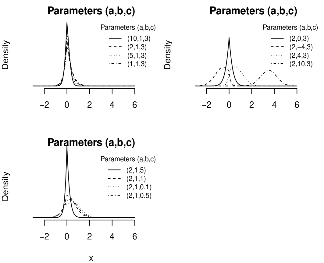
Figure 1: The Lasso density function is depicted for different parameter values. In the top left panel, parameter $a$ is varied while the other parameters are fixed. In the top right and bottom left panels, parameters $b$ and $c$ are varied, respectively, while the other parameters are fixed.

The MGF of the Lasso distribution is $M(t)=Z(a,b+t,c)/Z(a,b,c)$ and the calculation of the moments of the Lasso distribution via the MGF is algebraically cumbersome. See Section 11 of the Supplementary Materials for the derivation of the MGF. However, by expressing the Lasso distribution as a mixture of two truncated normal distributions, the moments can be calculated as $\mathbb{E}(X^{r})=(1-w)\cdot\mathbb{E}(A^{r})+w\cdot\mathbb{E}(B^{r}),$ where the mixing proportion is given by

$$w=\left[1+\frac{\Phi(\mu_{1}/\sigma)}{\phi(\mu_{1}/\sigma)}\frac{\phi(-\mu_{2}/\sigma)}{\Phi(-\mu_{2}/\sigma)}\right]^{-1},$$

where $A\sim TN_{+}(\mu_{1},\sigma^{2})$ and $B\sim TN_{-}(\mu_{2},\sigma^{2})$ are the positively truncated and negatively truncated normal distributions, respectively.

The CDF of the Lasso distribution is given by

$$P(x)=\mathcal{P}(X<x)=\left\{\begin{array}[]{ll}\displaystyle w\frac{\Phi\left(\frac{x-\mu_{2}}{\sigma}\right)}{\Phi(-\mu_{2}/\sigma)}&\mbox{if $x\leq 0$ and}\\[8.61108pt] \displaystyle 1-(1-w)\frac{\Phi(\frac{\mu_{1}-x}{\sigma})}{\Phi(\mu_{1}/\sigma)}&\mbox{if $x>0$}.\end{array}\right.$$

The inverse CDF of the Lasso distribution is given by

$$P^{-1}(u)=\left\{\begin{array}[]{ll}\mu_{2}+\sigma\Phi^{-1}[\Phi(-\mu_{2}/\sigma)u/w]&\mbox{if $u\leq w$ and}\\[8.61108pt] \mu_{1}-\sigma\Phi^{-1}[\Phi(\mu_{1}/\sigma)(1-u)/(1-w)]&\mbox{if $u>w$}.\end{array}\right.$$

Finally, the mode of the Lasso distribution is equal to $\mbox{max}(|b|-c,0)\cdot\mbox{sign}(b)/a$, where $\mbox{sign}(\cdot)$ is the sign function.

The R package BayesianLasso enables efficient and numerically stable sampling from the Lasso distribution by evaluating the inverse CDF using uniform random draws. To ensure robustness, particularly in the tails, the implementation incorporates safeguards against numerical issues such as overflow and underflow. A key component of this approach is the numerically stable evaluation of the Mill’s ratio, defined as $m(x)=\Phi(-x)/\phi(-x)$, which is used in computing the normalizing constant. Specifically, the package computes

$$v_{1}=\frac{c-\left|b\right|}{\sqrt{a}}\qquad\mbox{and}\qquad v_{2}=\frac{c+\left|b\right|}{\sqrt{a}},$$

and evaluates the normalizing constant as $Z=\left[m\left(v_{1}\right)+m\left(v_{2}\right)\right]/\sqrt{a}$. This combination of numerical stability and computational efficiency underpins the practical value of the package and is a key reason for its robustness in high-dimensional Bayesian inference.

3.1   Sampling from the Lasso distribution

Key quantities required for various expressions in the previous section include the computation of $Z$ and $w$. Additionally, special care must be taken when calculating the inverse CDF to prevent both overflow and underflow. To address these concerns, we define $v_{1}=\left[c-\left|b\right|\right]/\sqrt{a}$ and $v_{2}=\left[c+\left|b\right|\right]/\sqrt{a}$. The normalizing constant $Z$ can then be expressed as $Z=\left[m\left(v_{1}\right)+m\left(v_{2}\right)\right]/\sqrt{a}$. For negative inputs, i.e., $x<0$, the Mill’s ratio is $m\left(x\right)=\phi\left(x\right)^{-1}-m\left(-x\right)$. Since $v_{2}\geq 0$ and $v_{1}\geq 0$ when $\left|b\right|\leq c$, we can partition the definition of $Z$ into two cases

$$Z =\begin{cases}\frac{1}{\sqrt{a}}\left[m\left(v_{1}\right)+m\left(v_{2}\right)\right]&\left|b\right|\leq c\quad\mbox{and}\\ \frac{1}{\sqrt{a}}\left[\left(\phi\left(v_{1}\right)^{-1}-m\left(-v_{1}\right)\right)+m\left(v_{2}\right)\right]&\left|b\right|>c;\end{cases}$$

where both alternatives have the requirement for two Mill’s ratio calculations for positive parameters; this is a potential use case for a SIMD, which is short for single instruction/multiple data, vectorized implementation of the positive side of the Mill’s ratio.

The second component of $Z$ (for $\left|b\right|>c$) has an obvious potential overflow when $\left|v_{1}\right|$ is large. In such cases, it may be necessary to transition to logarithmic space to represent $\phi\left(v_{1}\right)$ to avoid underflow/overflow. However, unnecessary logarithmic computations should be avoided, as they are computationally expensive and can reduce numerical precision when not required. Marsaglia (2004) notes that the precision of evaluating the standard normal density function $\phi\left(x\right)$ and its tail probability deteriorates as $x$ increases, due to the limitations of computing $\exp(-x^{2}/2)$ in double-precision arithmetic. While the paper primarily examines values up to $x\approx 16$, it is also known that $\phi\left(x\right)$ effectively loses all precision for $x\geq 37$ , where the exponential term underflows to zero and the reciprocal overflows. Now, consider the case where $v_{1}<-37$, making overflow a concern. By definition, we have $37<-v_{1}<v_{2}$, which implies $m\left(37\right)>m\left(-v_{1}\right)>m\left(v_{2}\right)>0$. Since $m\left(37\right)\approx 0.027$, it follows that $-0.027<m\left(v_{2}\right)-m\left(-v_{1}\right)<0$. Within the limits of double precision, this difference becomes negligible due to rounding errors for $v_{1}\approx-9$, and certainly for $v_{1}<-37$, where $\phi\left(-37\right)<6\times 10^{-300}$. Consequently, $Z$ can be approximated as

$$Z \approx\frac{1}{\sqrt{a}}\left[\phi\left(v_{1}\right)^{-1}\right].$$

Thus, we can safely use the approximation $m\left(v_{1}\right)\approx\phi\left(v_{1}\right)^{-1}$ in such cases.

For a fast and accurate approximation of Mill’s ratio for positive arguments, we employ a degree $\left(8,9\right)$ rational polynomial optimized using the Remez algorithm (Reemtsen, 1990) over the interval $\left[0,600\right]$, achieving an accuracy of up to 12 significant figures. The leading coefficients of both the numerator and denominator are positive, ensuring that the approximation asymptotically converges to a small fraction. This stability allows the relative error to remain consistent, preserving 11 significant figures up to approximately $x\approx 2000$. Beyond this point, the precision gradually improves, as Mill’s ratio satisfies $m(x)\sim 1/x$ for large $x$.

Let

$$\begin{array}[]{c}p_{0}=46697.7602201933,\qquad p_{1}=69339.6909002865,\qquad p_{2}=50590.6980372328,\\ p_{3}=23184.62760379742,\qquad p_{4}=7236.31450136984,\qquad p_{5}=1572.136841909630,\\ p_{6}=232.9967987466022,\qquad p_{7}=21.74833514806325,\qquad\mbox{and}\quad p_{8}=1.000000000000095.\end{array}$$

and let

$$\begin{array}[]{c}q_{0}=37259.42190376593,\qquad q_{1}=85053.78630172011,\qquad q_{2}=89598.92885811838,\\ q_{3}=57370.93777717682,\qquad q_{4}=24713.27114352290,\qquad q_{5}=7467.311205544661,\\ q_{6}=1593.885178714749,\qquad q_{7}=233.9967987305447,\qquad q_{8}=21.74833514813385,\\ \end{array}$$

and $q_{9}=1$. Let

$$\widetilde{m}=\frac{p_{0}+x(p_{1}+x(p_{2}+x(p_{3}+x(p_{4}+x(p_{5}+x(p_{6}+x(p_{7}+xp_{8})))))))}{q_{0}+x(q_{1}+x(q_{2}+x(q_{3}+x(q_{4}+x(q_{5}+x(q_{6}+x(q_{7}+x(q_{8}+x))))))))}.$$

Our approximation of $m(x)$ for $x>0$ is then

$$m(x)=\left\{\begin{array}[]{ll}\widetilde{m}&\mbox{$x<1.75\times 10^{34}$}\\ 1/x&\mbox{otherwise.}\end{array}\right.$$

Next, we define

$$w_{1}=\frac{1}{1+m\left(v_{1}\right)m\left(v_{2}\right)^{-1}}\qquad\mbox{and}\qquad w_{2}=\frac{1}{1+m\left(v_{1}\right)^{-1}m\left(v_{2}\right)}.$$

As $v_{1}\rightarrow-\infty$, it follows that $m\left(v_{1}\right)\rightarrow\infty$, leading to $w_{1}\rightarrow 0$ and $w_{2}\rightarrow 1$. However, due to the dynamic range limitations of floating-point representation, $w_{1}$ is representable, whereas $w_{2}$ rounds to 1 for $v_{1}\lessapprox-5.5$, resulting in a loss of precision. Since floating-point arithmetic offers much better precision near zero than near one, using $w_{2}$ when $v_{1}\ll 0$ can introduce numerical errors. To mitigate this, we define

$$w=\begin{cases}w_{1}&\mbox{if }b\leq 0\mbox{ and}\\ w_{2}&\mbox{if }b>0,\end{cases}\qquad\mbox{and}\qquad 1-w=\begin{cases}w_{2}&\mbox{if }b\leq 0\mbox{ and}\\ w_{1}&\mbox{if }b>0.\end{cases}$$

Thus, a simple yet numerically stable rule is to work with $w$ when $b\leq 0$ and with $1-w$ when $b>0$.

The computation of $P^{-1}(u)$ is carried out in four distinct cases, determined by whether $u\leq w$ and whether $b>0$. First, the arguments of $\Phi^{-1}(\cdot)$ are carefully computed to prevent overflow. In extreme cases, underflow may still occur. When underflow is detected, the arguments of $\Phi^{-1}(\cdot)$ are instead computed on the logarithmic scale, and the asymptotic tail formula of Mächler (2022) is used to evaluate $\Phi^{-1}(\cdot)$ accurately.

4   Using the BayesianLasso package

To illustrate the functionality of the BayesianLasso package, we provide examples of its key functions, including density evaluation, cumulative distribution, random sampling, and quantile calculations.

4.1   Probability density function (PDF)

The function dlasso() computes the probability density function of the Lasso distribution for given parameters. The following example plots the density of a Lasso(2,1,3) distribution, shown as a solid black line in Figure 2.

library(BayesianLasso)# Define parametersa <- 2b <- 1c <- 3x <- seq(-3, 3, length = 1000)# Plot the density of Lasso(2,1,3)plot(x, dlasso(x, a, b, c, logarithm = FALSE), type = ’l’,     xlab = "x", ylab = "Density",     ylim = c(0, 2.25), yaxt = "n", bty = "n")

4.2   Cumulative distribution function (CDF)

The function plasso() calculates the cumulative distribution function of the Lasso distribution. Below, we compute the CDF at $x=-1$ for a $\text{Lasso}(2,1,3)$ distribution:

CDF_value <- plasso(-1, a, b, c)print(CDF_value)[1] 0.00176594

4.3   Random sampling from the Lasso distribution

To generate random samples from the Lasso distribution, we use rlasso(). The following example generates 100,000 samples and compares the empirical density with the theoretical density, as shown in Figure 2.

# Generate random samplessamples <- rlasso(100000, a, b, c)# Compare empirical and theoretical densityplot(x, dlasso(x, a, b, c, logarithm = F), type = ’l’, xlab = "x", ylab = "Density",     xlim = c(-2, 2), yaxt = "n", bty = "n")lines(density(samples), col = ’red’)legend("topright", legend = c("Theoretical", "Empirical"),       col = c("black", "red"), lty = 1, bty = "n")

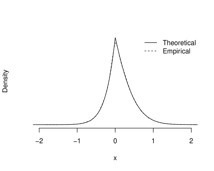
Figure 2: Theoretical and empirical densities for $\text{Lasso}(2,1,3)$. The theoretical density plot of $\text{Lasso}(2,1,3)$ using dlasso(x, a, b, c, logarithm = FALSE) is shown as a solid black line, and the empirical density is shown as a dashed line.

4.4   Quantile function

The qlasso() function computes quantiles of the Lasso distribution. Below, we compute the quantiles for probability values $p=\{0.1,0.3,0.6\}$:

p_values <- c(0.1, 0.3, 0.6)quantiles <- qlasso(p_values, a, b, c)print(quantiles)[1] -0.28183916 -0.04935763  0.16137104

In the next section, we incorporate the Lasso distribution into a Gibbs sampling algorithm as the full conditional distribution for the coefficients of the Lasso regression model.

5   Application of the Lasso distribution in Gibbs sampling

We modify the Gibbs sampler of Hans (2009) (henceforth Hans) by using the Lasso distribution as the full conditional distribution of the regression coefficients. We also consider a slightly modified version of the Gibbs sampler of Park and Casella (2008) (henceforth PC), as the alternative Gibbs sampler, by changing the representation of the auxiliary variable from (1) to (2).

Furthermore, these Gibbs samplers are based on the prior $\lambda^{2}\sim\mbox{Gamma}(u,v)$ which differs from Hans (2009) which places this prior on $\lambda$ (which is conjugate) rather than $\lambda^{2}$ (which is not). Therefore, we employ a slice sampler to draw from the full conditional distribution of $\lambda^{2}$ (Neal, 2003). All methods are implemented in the same programming language and executed on the same computer, ensuring that the primary distinction lies in the choice of Gibbs samplers used to fit the model.

5.1   Hans Gibbs sampler

As mentioned earlier, the standard Gibbs sampler proposed by Hans (2009) relies on the fact that the full conditional distribution for each $\beta_{j}$ is given by (3), and Hans (2009) notes that $p(\beta_{j}|{\mathcal{D}},{\boldsymbol{\beta}}_{-j},\sigma^{2},\lambda^{2})$ can be represented as a mixture of two truncated normal distributions. This is not a well-known distribution to sample. However, we show care needs to be taken to avoid numerical problems using this representation.

To facilitate sampling from the kernel in (3), we utilize the Lasso distribution ($\mbox{Lasso}(a,b,c)$), which we introduced in Section 3. We also employ the efficient and numerically stable sampling method developed in Section 3.1 to draw samples from this distribution. Notably, while the Hans sampler is specifically designed for the Lasso distribution, it is difficult to extend to other response types or alternative penalty structures.

Algorithm 1 presents our modified version of Hans’ Gibbs sampling algorithm, where we model $\lambda^{2}\sim\mbox{Gamma}(u,v)$ instead of $\lambda\sim\mbox{Gamma}(u,v)$. Unlike the original method in Hans (2009), which employs conjugate sampling for $\lambda$ and rejection sampling for $\sigma^{2}$, our approach collapses the auxiliary variable $a_{j}$ to improve mixing and utilizes slice sampling for both $\sigma^{2}\mid{\mathcal{D}},{\boldsymbol{\beta}},\lambda^{2}$ and $\lambda^{2}\mid{\mathcal{D}},{\boldsymbol{\beta}},\sigma^{2}$ (Neal, 2003). Notably, the same slice sampler is applied to both parameters, as their full conditional distributions are inverse transformations of each other.

Algorithm 1 Modified Hans Gibbs sampler

1:Inputs: ${\bf y}$, ${\bf X}$, $\widetilde{a}>0$, $\widetilde{b}>0$, $u>0$, $v>0$, ${\boldsymbol{\beta}}^{(0)}={\bf 0}_{p}$, $\sigma^{2(0)}>0$, $\lambda^{(0)}>0$;

2:for $i=1,\ldots,\textit{N}$ do

3:  ${\boldsymbol{\beta}}^{(i)}\leftarrow{\boldsymbol{\beta}}^{(i-1)}$;

4:  if $n>p$ then

5:   ${\boldsymbol{\delta}}\leftarrow({\bf X}^{T}{\bf X}){\boldsymbol{\beta}}^{(i)}$;

6:   for $j=1,\ldots,\textit{p}$ do

7:     ${\boldsymbol{\delta}}\leftarrow{\boldsymbol{\delta}}-{\bf X}_{j}\beta_{j}^{(i)}$;

8:     $\displaystyle\beta^{(i)}_{j}\sim\text{Lasso}\left(\frac{\|{\bf X}_{j}\|_{2}^{2}}{\sigma^{2(i-1)}},\frac{({\bf X}^{T}{\bf y})_{j}-\delta_{j}}{\sigma^{2(i-1)}},\frac{\lambda^{(i-1)}}{\sigma^{(i-1)}}\right);$

9:     ${\boldsymbol{\delta}}\leftarrow{\bf r}+{\bf X}_{j}\beta_{j}^{(i)}$;

10:   end for

11:   $\mbox{RSS}\leftarrow\|{\bf y}\|_{2}^{2}-2{\bf y}^{T}{\bf X}{\boldsymbol{\beta}}_{j}^{(i)}+({\boldsymbol{\beta}}_{j}^{(i)})^{T}{\bf X}^{T}{\bf X}{\boldsymbol{\beta}}_{j}^{(i)}$;

12:  else

13:   ${\bf y}\leftarrow{\bf X}{\boldsymbol{\beta}}^{(i)}$;

14:   for $j=1,\ldots,\textit{p}$ do

15:     ${\bf r}_{j}\leftarrow{\bf y}-(\widehat{{\bf y}}-{\bf X}_{j}\beta^{(i-1)}_{j});$

16:     $\displaystyle\beta^{(i)}_{j}\sim\text{Lasso}\left(\frac{\|{\bf X}_{j}\|_{2}^{2}}{\sigma^{2(i-1)}},\frac{{\bf X}_{j}^{T}{\bf r}_{j}}{\sigma^{2(i-1)}},\frac{\lambda^{(i-1)}}{\sigma^{(i-1)}}\right);$

17:     $\widehat{\bf y}\leftarrow\widehat{\bf y}+{\bf X}_{j}(\beta^{(i)}_{j}-\beta^{(i-1)}_{j})$;

18:   end for

19:   $\mbox{RSS}\leftarrow\|{\bf y}-\widehat{{\bf y}}\|_{2}^{2}$;

20:  end if

21:  Use slice sampling to sample $\sigma^{2(i)}$ from the density

$$p(\sigma^{2}|{\mathcal{D}},{\boldsymbol{\beta}}^{(i)},\lambda^{2(i-1)})\propto\exp\left[(\widetilde{a}+\tfrac{n+p}{2}+1)\log(\sigma^{2})-\left(\widetilde{b}+\tfrac{1}{2}\mbox{RSS}\right)\sigma^{-2}-\tfrac{\lambda^{(i-1)}}{\sigma}\|{\boldsymbol{\beta}}^{(i)}\|_{1}\right];$$

22:  Use slice sampling to sample $\lambda^{2(i)}$ from the density

$$p(\lambda^{2}|{\mathcal{D}},{\boldsymbol{\beta}}^{(i)},\sigma^{2(i)})\propto\exp\left[\left(u+\tfrac{p}{2}-1\right)\log(\lambda^{2})-v\lambda^{2(i-1)}-\tfrac{\lambda}{\sigma^{(i)}}\|{\boldsymbol{\beta}}^{(i)}\|_{1}\right].$$

23:end for

In Algorithm 1, the quantity ${\bf r}_{j}$ is analogous to the partial residuals used in coordinate descent methods for optimizing the Lasso objective function (see, e.g., Hastie et al., 2015, Section 5.4.2). However, rather than computing the mode of $\beta_{j}|{\mathcal{D}},{\boldsymbol{\beta}}_{-j},\sigma^{2}$ as done in coordinate descent, we draw samples from its distribution.

Hans (2009) does not discuss the computational costs of the Gibbs samplers presented there. In contrast, our Algorithm 1 avoids matrix inversion, and as shown in Algorithm 1, sampling each variable requires $O(\min(n,p))$ time. Moreover, Algorithm 1 accommodates both the $n>p$ and $p>n$ settings, running in $O(Np\min(n,p))$ time. This complexity suggests that Algorithm 1 may be computationally more efficient than Algorithm 2 for datasets where $p>n$ or where $n>p$ but $n$ is of smaller order than $p^{2}$.

Note that our BayesianLasso package implements the modified Hans sampler via the function Modified_Hans_Gibbs(). In this function, ${\bf X}$ and ${\bf y}$ represent the covariate matrix and the response vector, respectively. The arguments a1, b1, u1, and v1 correspond to the hyperparameters of the priors for $\sigma^{2}$ and $\lambda^{2}$. The total number of MCMC iterations is specified by nsamples, and the initial values for ${\boldsymbol{\beta}}$, $\sigma^{2}$ and $\lambda^{2}$ are set via beta_init, sigma2_init and lambda_init, respectively. The argument verbose controls whether the sampling progress is printed during execution.

5.2   PC Gibbs sampler

Our modified PC Gibbs sampler is presented in Algorithm 2, which consists of a four-block Gibbs sampling scheme for estimating the model parameters, auxiliary variables, and the tuning parameter $\lambda^{2}$. Specifically, it involves sampling from the full conditional distributions: $[{\boldsymbol{\beta}}|{\mathcal{D}},\sigma^{2},\lambda^{2},{\bf a}]$, $[\sigma^{2}|{\mathcal{D}},{\boldsymbol{\beta}},\lambda^{2},{\bf a}]$, $[\lambda^{2}|{\mathcal{D}},{\boldsymbol{\beta}},\sigma^{2},{\bf a}]$, and $[{\bf a}|{\mathcal{D}},{\boldsymbol{\beta}},\sigma^{2},\lambda^{2}]$. The time complexity of Algorithm 2 is $O(np^{2}+Np^{3})$ where $N$ is the number of MCMC samples, assuming that quantities such as ${\bf X}^{T}{\bf X}$, ${\bf X}^{T}{\bf y}$, and $\|{\bf y}\|_{2}^{2}$ are precomputed outside the main loop. A key advantage of this algorithm is that the inner loop’s time complexity is independent of $n$, making it particularly beneficial when $n$ is large. However, the algorithm scales cubically with $p$, as it requires computing a matrix square root—typically via Cholesky factorization or eigen-decomposition—to sample ${\boldsymbol{\beta}}^{(i)}$ (Golub and van Loan, 2013).

Algorithm 2 Modified PC Gibbs sampler

1:Inputs: ${\bf y}$, ${\bf X}$, $\widetilde{a}>0$, $\widetilde{b}>0$, $u>0$, $v>0$, $\lambda^{2}>0$, and $\sigma^{2(0)}>0$.

2:${\bf a}^{(0)}={\bf 1}_{n}$;

3:for $i=1,\ldots,\textit{N}$ do

4:  ${\bf A}\leftarrow\text{diag}({\bf a}^{(i-1)})$;

5:  ${\boldsymbol{\beta}}^{(i)}\sim N_{p}\left[({\bf X}^{T}{\bf X}+\lambda^{2(i-1)}{\bf A})^{-1}{\bf X}^{T}{\bf y},\sigma^{2(i-1)}({\bf X}^{T}{\bf X}+\lambda^{2(i-1)}{\bf A})^{-1}\right]$;

6:  $\sigma^{2(i)}\sim\text{IG}\left(\widetilde{a}+\tfrac{n+p}{2},\widetilde{b}+\tfrac{1}{2}\|{\bf y}\|_{2}^{2}-{\bf y}^{T}{\bf X}{\boldsymbol{\beta}}^{(i)}+\tfrac{1}{2}({\boldsymbol{\beta}}^{(i)})^{T}({\bf X}^{T}{\bf X}+\lambda^{2(i-1)}{\bf A}){\boldsymbol{\beta}}^{(i)}\right)$;

7:  $\displaystyle\lambda^{2(i)}\sim\text{Gamma}\left(u+\frac{p}{2},v+\frac{({\boldsymbol{\beta}}^{(i)})^{T}{\bf A}{\boldsymbol{\beta}}^{(i)}}{2\sigma^{2(i)}}\right)$;

8:  for $j=1,\ldots,\textit{p}$ do

9:   $\displaystyle a^{(i)}_{j}\sim\text{Inverse-Gaussian}\left(\frac{\sigma^{(i)}}{\lambda|\beta_{j}^{(i-1)}|},1\right)$.

10:  end for

11:end for

Note that our BayesianLasso package implements the modified PC sampler via the function Modified_PC_Gibbs(). In this function, ${\bf X}$ and ${\bf y}$ represent the covariate matrix and the response vector, respectively. The arguments a1, b1, u1, and v1 correspond to the hyperparameters of the priors for $\sigma^{2}$ and $\lambda^{2}$. The total number of MCMC iterations is specified by nsamples, and the initial values for $\sigma^{2}$ and $\lambda^{2}$ are set via sigma2_init and lambda_init. The argument verbose controls whether the sampling progress is printed during execution.

6   Performance comparison on benchmark datasets

In this section, we compare the performance of our modified Hans sampler with our modified PC Gibbs sampler, as well as the R packages monomvn, bayeslm, rstan, and bayesreg (Gramacy, 2024; He et al., 2022; Stan Development Team, 2020; Makalic and Schmidt, 2016). The comparison is based on several benchmark datasets that represent a diverse range of scenarios where $n>p$. Specifically, we consider the Diabetes dataset with all pairwise interactions of the original variables (referred to as Diabetes²) from the lars package (Efron et al., 2004; Hastie and Efron, 2022), with $n=442$ and $p=55$; the Kakadu dataset with all pairwise interactions (Kakadu²) from the Ecdat package (Croissant and Graves, 2022), with $n=1827$ and $p=252$; and the Crime dataset from the UCI Machine Learning Repository with $n=2215$ and $p=98$ (Redmond, 2002).

The impact of autocorrelation within the chains on estimation uncertainty can be quantified using the effective sample size (ESS). We compute ESS using the ess_bulk() function from the posterior package in R (Bürkner et al., 2023; Vehtari et al., 2021). To evaluate the efficiency of our proposed MCMC approach relative to the modified PC Gibbs sampler and the aforementioned R packages, we use the following metric

$$\mbox{Efficiency}=\frac{\mbox{ESS}}{\mbox{time}};$$

where time represents execution time in seconds. Additionally, we assess whether the MCMC samples have reached a stationary distribution and exhibit adequate mixing using Gelman and Rubin’s convergence diagnostic, $\widehat{R}$ (Gelman and Rubin, 1992). We assess whether the outputs from each chain are indistinguishable by examining the scale reduction factor, considering values below 1.1 as an indication of convergence.

We also evaluate the quality of mixing using the ratio

$$\mbox{Mix \%}=100\times\frac{\mbox{ESS}}{N}$$

where $N$ represents the total number of samples. We use 1,000 burn-in samples followed by 5,000 samples for inference. The computations were performed on an Apple M1 Pro with 12 cores and 16 GB of RAM. The Gibbs sampler methods were implemented in the R programming language (version 4.4.2), leveraging the computational efficiency of the Rcpp (version 1.0.13-1) (Eddelbuettel et al., 2024a; Eddelbuettel and François, 2011; Eddelbuettel, 2013; Eddelbuettel and Balamuta, 2018) and RcppArmadillo (version 14.2.2-1) (Eddelbuettel and Sanderson, 2014; Eddelbuettel et al., 2024b) packages.

Table 1 presents the mixing percentages, sampling efficiencies, and elapsed times (in seconds) for the modified Hans and PC Gibbs samplers applied to the benchmark datasets Diabetes², Kakadu², and Crime. It is important to note that the Gelman–Rubin diagnostic $\widehat{R}$ for each model parameter was below 1.01, indicating convergence, and the effective sample size (ESS) for ${\boldsymbol{\beta}}$ corresponds to the median of the ESS values for the $p$-dimensional vector ${\boldsymbol{\beta}}$. The results indicate that the modified Hans sampler is the most efficient for sampling $\sigma^{2}$ and $\lambda^{2}$ in the Diabetes² and Kakadu² datasets. It is also the most efficient for sampling ${\boldsymbol{\beta}}$ in the Kakadu², and the second most efficient—after the modified PC sampler—for sampling ${\boldsymbol{\beta}}$ in the Diabetes² dataset. Furthermore, the modified Hans sampler achieves the shortest computation time in the Diabetes² and Crime datasets. Note that monomvn was extremely slow on the Kakadu² dataset. Therefore, its output is reported as NA, as it was not within a comparable range of performance with the other samplers.

		${\boldsymbol{\beta}}$	Eff	$\sigma^{2}$	Eff	$\lambda^{2}$	Eff	Time
Dataset	Method	Mix %	($\times 10^{2}$)	Mix %	($\times 10^{2}$)	Mix %	($\times 10^{2}$)	(s)
Diabetes2	Hans	26.3	3914.6	69.9	10388.5	25.2	3746.6	1.2
	PC	78.2	4939.9	66.4	4191.9	21.7	1372.8	3.0
	monomvn	99.9	79.2	100.0	79.6	100.0	80.1	239.6
	bayeslm	11.7	1657.9	49.9	6587.3	4.0	539.5	1.4
	rstan	98.9	158.2	100.0	162.0	98.3	157.2	118.7
	bayesreg	76.4	2043.4	60.8	1627.3	17.8	477.0	7.0
Kakadu2	Hans	18.9	700.6	73.1	2702.3	4.8	178.5	5.1
	PC	85.5	41.8	71.0	34.7	8.8	4.3	388.1
	monomvn	NA	NA	NA	NA	NA	NA	NA
	bayeslm	14.7	186.6	49.6	628.1	2.9	37.0	3.1
	rstan	98.5	22.6	96.1	22.1	95.0	21.8	173.7
	bayesreg	84.3	190.3	60.5	136.6	4.2	9.5	17.7
Crime	Hans	2.9	229.3	72.6	5740.9	4.7	377.5	0.5
	PC	86.5	555.2	90.7	582.7	30.1	193.2	6.2
	monomvn	97.9	5.8	95.8	5.7	96.5	5.7	666.9
	bayeslm	2.8	142.7	81.8	4042.3	7.9	391.0	0.8
	rstan	97.9	28.2	100.0	28.8	100.0	31.1	138.8
	bayesreg	85.9	617.0	80.6	578.9	29.7	213.6	5.5

Table 1: Mixing percentages, efficiencies, and computation times (in seconds) for each dataset using the Hans and PC Gibbs samplers from the BayesianLasso package, as well as the R packages monomvn, bayeslm, rstan, and bayesreg.

7   Discussion

This paper introduces the BayesianLasso R package, which provides a comprehensive and computationally efficient implementation of Bayesian Lasso regression based on a newly defined Lasso distribution. The package encapsulates recent methodological advances by offering implementations of both the modified Hans and PC Gibbs samplers, tailored to exploit the distributional structure of the Lasso prior.

Central to the package is the formal development of the Lasso distribution, which we establish as a member of the exponential family. We derive key theoretical properties—including the probability density function, cumulative distribution function, moments, and a numerically stable inverse-CDF sampling method—which underpin the samplers implemented in the package. In particular, the Lasso distribution serves as the full conditional distribution for regression coefficients in the proposed Gibbs sampling framework.

The BayesianLasso package is designed with usability and extensibility in mind, offering an accessible interface for researchers and practitioners to fit Bayesian Lasso models in regression settings where $n>p$. The package also provides utility functions for working directly with the Lasso distribution, including density evaluation, random sampling, and cumulative probability calculations.

Our empirical evaluations demonstrate that the modified Hans sampler achieves efficient mixing for sampling from $\sigma^{2}$ and $\lambda^{2}$ in the Diabetes² and Kakadu² datasets, and it also achieves efficient computational scalability in the Diabetes² and Crime datasets, making it a practical tool for posterior inference. By integrating this method into an easy-to-use R package, we aim to lower the barrier to adoption and encourage broader use of Lasso-based Bayesian modeling in applied statistical work.

8   Code availability

The R package BayesianLasso implementing the methods described in this paper is available at:
https://github.com/garthtarr/BayesianLasso

9   Competing interests

The authors declare that they have no conflict of interest.

John T. Ormerod
School of Mathematics and Statistics, University of Sydney
Sydney
Australia
john.ormerod@sydney.edu.au

Mohammad Javad Davoudabadi
School of Mathematics and Statistics, University of Sydney
Sydney
Australia
mohammad.davoudabadi@sydney.edu.au

Garth Tarr
School of Mathematics and Statistics, University of Sydney
Sydney
Australia
garth.tarr@sydney.edu.au

Samuel Muller
Faculty of Science and Engineering, Macquarie University
Sydney
Australia
samuel.muller@mq.edu.au

Jonathon Tidswell
School of Mathematics and Statistics, University of Sydney
Sydney
Australia
jonathon.tidswell@sydney.edu.au

10   Derivation of the full conditional for each $\beta_{j}$

Consider $p({\bf y}|\boldsymbol{\beta},{\bf a})$, $p(\boldsymbol{\beta}|{\bf a})$, $p({\bf a})$, $p(\sigma^{2})$, and $p(\lambda^{2})$ are the likelihood function, and the priors of $\boldsymbol{\beta}$, ${\bf a}$, $\sigma^{2}$, and $\lambda^{2}$, respectively. The log of the full joint distribution is proportional to

$$\log p(\boldsymbol{\beta},\sigma^{2},\lambda^{2},{\bf a}) =\log\big{(}p({\bf y}|\boldsymbol{\beta,{\bf a}})p(\boldsymbol{\beta}|{\bf a})p({\bf a})p(\sigma^{2})p(\lambda^{2})\big{)}$$

$$\propto-\frac{1}{2\sigma^{2}}\Big{[}{\bf y}^{T}{\bf y}-2{\bf y}^{T}\mathbf{X}^{T}\boldsymbol{\beta}+\boldsymbol{\beta}^{T}\mathbf{X}^{T}\mathbf{X}\boldsymbol{\beta}+\lambda^{2}\boldsymbol{\beta}^{T}{\bf A}\boldsymbol{\beta}\Big{]}$$

$$\quad\quad{}-\frac{\sum_{i=1}^{p}a_{i}}{2}-2\sum_{i=1}^{p}a_{i}-\sum_{i=1}^{p}\frac{1}{2a_{i}}+\mbox{constant};$$

where ${\bf a}=(a_{1},...,a_{p})$ and ${\bf A}=\text{diag}({\bf a}^{-1})$. After integrating out ${\bf a}$ from the above proportion, the marginal distribution of $\beta_{j}$ is as follows

$$\log p(\beta_{j})\propto-\frac{\parallel\mathbf{X}_{j}\parallel^{2}_{2}}{2\sigma^{2}}\beta_{j}^{2}+\frac{\mathbf{X}_{j}^{T}({\bf y}-\mathbf{X}_{-j}\boldsymbol{\beta}_{-j})}{\sigma^{2}}\beta_{j}-\frac{\lambda^{2}}{\sigma}|\beta_{j}|;$$

which is a univariate Lasso distribution with parameters $a=\frac{\parallel\mathbf{X}_{j}\parallel^{2}_{2}}{\sigma^{2}}$, $b=\frac{\mathbf{X}_{j}^{T}({\bf y}-\mathbf{X}_{-j}\boldsymbol{\beta}_{-j})}{\sigma^{2}}$, and $c=\frac{\lambda^{2}}{\sigma}$.

11   Derivation of the distributional properties of the Lasso distribution

If $X\sim\mbox{Lasso}(a,b,c)$ with then it has density given by

$$p(X,a,b,c)=Z^{-1}\exp\left(-\tfrac{1}{2}aX^{2}+bX-c|X|\right)$$

where $Z$ is the normalizing constant. Then

$$\begin{array}[]{rl}Z(a,b,c)&=\int_{-\infty}^{\infty}\exp\left[-\tfrac{1}{2}aX^{2}+bX-c|X|\right]dx\\[8.61108pt] &=\int_{0}^{\infty}\exp\left[-\tfrac{1}{2}aX^{2}+(b-c)X\right]dx+\int_{-\infty}^{0}\exp\left[-\tfrac{1}{2}aX^{2}+(b+c)X\right]dx\\[8.61108pt] &=\int_{0}^{\infty}\exp\left[-\frac{(X-\mu_{1})^{2}}{2\sigma^{2}}+\frac{\mu_{1}^{2}}{2\sigma^{2}}\right]dx+\int_{-\infty}^{0}\exp\left[-\frac{(X-\mu_{2})^{2}}{2\sigma^{2}}+\frac{\mu_{2}^{2}}{2\sigma^{2}}\right]dx\\[8.61108pt] &=\sqrt{2\pi\sigma^{2}}\left[\exp\left\{\frac{\mu_{1}^{2}}{2\sigma^{2}}\right\}\int_{0}^{\infty}\phi(x;\mu_{1},\sigma^{2})dx+\exp\left\{\frac{\mu_{2}^{2}}{2\sigma^{2}}\right\}\int_{-\infty}^{0}\phi(x;\mu_{2},\sigma^{2})dx\right]\\[8.61108pt] &=\sqrt{2\pi\sigma^{2}}\left[\exp\left\{\frac{\mu_{1}^{2}}{2\sigma^{2}}\right\}\left\{1-\Phi(-\mu_{1}/\sigma)\right\}+\exp\left\{\frac{\mu_{2}^{2}}{2\sigma^{2}}\right\}\left\{\Phi(-\mu_{2}/\sigma)\right\}\right]\\[8.61108pt] &=\sqrt{2\pi\sigma^{2}}\left[\exp\left(\frac{\mu_{1}^{2}}{2\sigma^{2}}\right)\Phi\left(\frac{\mu_{1}}{\sigma}\right)+\exp\left(\frac{\mu_{2}^{2}}{2\sigma^{2}}\right)\Phi\left(\frac{-\mu_{2}}{\sigma}\right)\right]\\[8.61108pt] &=\sigma\left[\frac{\Phi(\mu_{1}/\sigma)}{\phi(\mu_{1}/\sigma)}+\frac{\Phi(-\mu_{2}/\sigma)}{\phi(-\mu_{2}/\sigma)}\right]\end{array}$$

where $\mu_{1}=(b-c)/a$, $\mu_{2}=(b+c)/a$ and $\sigma^{2}=1/a$.

The MGF of the Lasso distribution is

$$M(t)=\mathbb{E}(\exp(tX)) =Z(a,b,c)^{-1}\int\exp(tX)\exp(\frac{-a}{2}X^{2}+bX-c|X|)dx$$

$$=Z(a,b,c)^{-1}\int\exp(\frac{-a}{2}X^{2}+(b+t)X-c|X|)dx$$

$$=\frac{Z(a,b+t,c)}{Z(a,b,c)}Z(a,b+t,c)^{-1}\int\exp(\frac{-a}{2}X^{2}+(b+t)X-c|X|)dx$$

$$=\frac{Z(a,b+t,c)}{Z(a,b,c)}.$$

The moments of the Lasso distribution are:

$$\begin{array}[]{rl}\mathbb{E}(X^{r})&=Z^{-1}\int_{-\infty}^{\infty}X^{r}\exp\left[-\tfrac{1}{2}aX^{2}+bX-c|X|\right]dx\\[8.61108pt] &=Z^{-1}\int_{0}^{\infty}X^{r}\exp\left[-\tfrac{1}{2}aX^{2}+(b-c)X\right]dx+\int_{-\infty}^{0}X^{r}\exp\left[-\tfrac{1}{2}aX^{2}+(b+c)X\right]dx\\[8.61108pt] &=Z^{-1}\sqrt{2\pi\sigma^{2}}\exp\left(\frac{\mu_{1}^{2}}{2\sigma^{2}}\right)\int_{0}^{\infty}X^{r}\phi(x;\mu_{1},\sigma^{2})dx+\sqrt{2\pi\sigma^{2}}\exp\left(\frac{\mu_{2}^{2}}{2\sigma^{2}}\right)\int_{-\infty}^{0}X^{r}\phi(x;\mu_{2},\sigma^{2})dx\par\\[8.61108pt] &=\frac{\sigma}{Z}\left[\frac{\Phi(\mu_{1}/\sigma)}{\phi(\mu_{1}/\sigma)}\frac{\int_{0}^{\infty}X^{r}\phi(x;\mu_{1},\sigma^{2})dx}{\Phi(\mu_{1}/\sigma)}+\frac{\Phi(-\mu_{2}/\sigma)}{\phi(-\mu_{2}/\sigma)}\frac{\int_{-\infty}^{0}X^{r}\phi(x;\mu_{2},\sigma^{2})dx}{\Phi(\mu_{2}/\sigma)}\right]\par\\[17.22217pt] &=\frac{\sigma}{Z}\left[\frac{\Phi(\mu_{1}/\sigma)}{\phi(\mu_{1}/\sigma)}\mathbb{E}(A^{r})+\frac{\Phi(-\mu_{2}/\sigma)}{\phi(-\mu_{2}/\sigma)}\mathbb{E}(B^{r})\right]\par\\[17.22217pt] &=\frac{\sigma}{\sigma\left[\frac{\Phi(\mu_{1}/\sigma)}{\phi(\mu_{1}/\sigma)}+\frac{\Phi(-\mu_{2}/\sigma)}{\phi(-\mu_{2}/\sigma)}\right]}\left[\frac{\Phi(\mu_{1}/\sigma)}{\phi(\mu_{1}/\sigma)}\mathbb{E}(A^{r})+\frac{\Phi(-\mu_{2}/\sigma)}{\phi(-\mu_{2}/\sigma)}\mathbb{E}(B^{r})\right]\\[17.22217pt] &=\left[\frac{\frac{\Phi(\mu_{1}/\sigma)}{\phi(\mu_{1}/\sigma)}}{\left[\frac{\Phi(\mu_{1}/\sigma)}{\phi(\mu_{1}/\sigma)}+\frac{\Phi(-\mu_{2}/\sigma)}{\phi(-\mu_{2}/\sigma)}\right]}\mathbb{E}(A^{r})+\frac{\frac{\Phi(-\mu_{2}/\sigma)}{\phi(-\mu_{2}/\sigma)}}{\left[\frac{\Phi(\mu_{1}/\sigma)}{\phi(\mu_{1}/\sigma)}+\frac{\Phi(-\mu_{2}/\sigma)}{\phi(-\mu_{2}/\sigma)}\right]}\mathbb{E}(B^{r})\right]\\[17.22217pt] &=(1-w)\mathbb{E}(A^{r})+w\mathbb{E}(B^{r})\par\end{array}$$

where $A\sim TN_{+}(\mu_{1},\sigma^{2})$, $B\sim TN_{-}(\mu_{2},\sigma^{2})$ and $TN_{+}$ is denotes the positively truncated normal distribution.

If $x\leq 0$ the CDF is given by

$$\begin{array}[]{rl}P(X<x)&=Z^{-1}\int_{-\infty}^{x}\exp\left[-\tfrac{1}{2}at^{2}+(b+c)t\right]dt\\[8.61108pt] &=Z^{-1}\sqrt{2\pi\sigma^{2}}\exp\left(\frac{\mu_{2}^{2}}{2\sigma^{2}}\right)\int_{-\infty}^{x}\phi(t;\mu_{2},\sigma^{2})dt\\[8.61108pt] &=Z^{-1}\sqrt{2\pi\sigma^{2}}\exp\left(\frac{\mu_{2}^{2}}{2\sigma^{2}}\right)\Phi\left(\frac{x-\mu_{2}}{\sigma}\right)\\[8.61108pt] &=\frac{\sigma}{Z}\frac{\Phi\left(\frac{x-\mu_{2}}{\sigma}\right)}{\phi(-\mu_{2}/\sigma)}\\[8.61108pt] &=w\frac{\Phi\left(\frac{x-\mu_{2}}{\sigma}\right)}{\Phi(-\mu_{2}/\sigma)}\par\end{array}$$

and if $x>0$ we have

$$\begin{array}[]{rl}P(X<x)&=Z^{-1}\int_{-\infty}^{x}\exp\left(-\tfrac{1}{2}at^{2}+bt-c|t|\right)dt\\[8.61108pt] &=Z^{-1}\sqrt{2\pi\sigma^{2}}\left[\exp\left(\frac{\mu_{1}^{2}}{2\sigma^{2}}\right)\int_{0}^{x}\phi(t;\mu_{1},\sigma^{2})dt+\exp\left(\frac{\mu_{2}^{2}}{2\sigma^{2}}\right)\Phi\left(\frac{-\mu_{2}}{\sigma}\right)\right]\\[8.61108pt] &=\frac{\sigma}{Z}\left[\frac{\Phi\left(\frac{x-\mu_{1}}{\sigma}\right)-\Phi\left(\frac{-\mu_{1}}{\sigma}\right)}{\phi(\mu_{1}/\sigma)}+\frac{\Phi\left(-\mu_{2}/\sigma\right)}{\phi(-\mu_{2}/\sigma)}\right]\\[8.61108pt] &=\displaystyle 1-(1-w)\frac{\Phi(\frac{\mu_{1}-x}{\sigma})}{\Phi(\mu_{1}/\sigma)}.\par\end{array}$$

For the inverse CDF, we again have two cases. Let $u=P(X<x)$. When

$$u\leq\frac{\sigma}{Z}\frac{\Phi\left(-\mu_{2}/\sigma\right)}{\phi(-\mu_{2}/\sigma)}=w$$

we solve

$$u=\frac{\sigma\Phi\left(\frac{x-\mu_{2}}{\sigma}\right)}{Z\phi(-\mu_{2}/\sigma)}$$

for $x$ to obtain

$$x=\mu_{2}+\sigma\,\Phi^{-1}\left[(Z/\sigma)\phi(-\mu_{2}/\sigma)u\right]=\mu_{2}+\sigma\,\Phi^{-1}\left[\Phi(-\mu_{2}/\sigma)u/w\right].$$

When

$$u>\frac{\sigma}{Z}\frac{\Phi\left(-\mu_{2}/\sigma\right)}{\phi(-\mu_{2}/\sigma)}=w$$

we need to solve

$$u=\displaystyle 1-(1-w)\frac{\Phi(\frac{\mu_{1}-x}{\sigma})}{\Phi(\mu_{1}/\sigma)}$$

for $x$ to obtain

$$x=\mu_{1}-\sigma\,\Phi^{-1}\left[\Phi(\mu_{1}/\sigma)(1-u)/(1-w)\right].$$

The Lasso distribution belongs to the exponential family distributions based on the following in which ${\boldsymbol{\theta}}=(a,b,c)$ is the set of parameters

$$p(X|{\boldsymbol{\theta}}) =h(X)\exp\left[{\boldsymbol{\nu}}({\boldsymbol{\theta}})\textbf{T}(X)-\mathbb{A}({\boldsymbol{\theta}})\right]$$

$$=\exp\left[-\tfrac{1}{2}aX^{2}+bX-c|X|-\left\{\log\left(\frac{\Phi(\mu_{1}/\sigma)}{\phi(\mu_{1}/\sigma)}+\frac{\Phi(-\mu_{2}/\sigma)}{\phi(-\mu_{2}/\sigma)}\right)+\log(\sigma)\right\}\right],$$

where

$$\begin{array}[]{c}{\boldsymbol{\nu}}({\boldsymbol{\theta}})=(-\frac{1}{2}a,b,-c),\quad h(X)=1,\quad\textbf{T}(X)=(X^{2},X,|X|),\quad\text{and}\\ \displaystyle\mathbb{A}({\boldsymbol{\theta}})=\log\left[\frac{\Phi(\mu_{1}/\sigma)}{\phi(\mu_{1}/\sigma)}+\frac{\Phi(-\mu_{2}/\sigma)}{\phi(-\mu_{2}/\sigma)}\right]+\log(\sigma).\end{array}$$

References

- Bürkner et al. (2023) P.-C. Bürkner, J. Gabry, M. Kay, and A. Vehtari. posterior: Tools for working with posterior distributions, 2023. URL https://mc-stan.org/posterior/. R package version 1.4.1.
- Croissant and Graves (2022) Y. Croissant and S. Graves. Ecdat: Data Sets for Econometrics, 2022. URL https://CRAN.R-project.org/package=Ecdat. R package version 0.4-2.
- Eddelbuettel (2013) D. Eddelbuettel. Seamless R and C++ Integration with Rcpp. Springer, New York, 2013. doi: 10.1007/978-1-4614-6868-4. ISBN 978-1-4614-6867-7.
- Eddelbuettel and Balamuta (2018) D. Eddelbuettel and J. J. Balamuta. Extending R with C++: A Brief Introduction to Rcpp. The American Statistician, 72(1):28–36, 2018. doi: 10.1080/00031305.2017.1375990.
- Eddelbuettel and François (2011) D. Eddelbuettel and R. François. Rcpp: Seamless R and C++ integration. Journal of Statistical Software, 40(8):1–18, 2011. doi: 10.18637/jss.v040.i08.
- Eddelbuettel and Sanderson (2014) D. Eddelbuettel and C. Sanderson. Rcpparmadillo: Accelerating R with high-performance C++ linear algebra. Computational Statistics and Data Analysis, 71:1054–1063, March 2014. doi: 10.1016/j.csda.2013.02.005.
- Eddelbuettel et al. (2024a) D. Eddelbuettel, R. Francois, J. Allaire, K. Ushey, Q. Kou, N. Russell, I. Ucar, D. Bates, and J. Chambers. Rcpp: Seamless R and C++ Integration, 2024a. URL https://CRAN.R-project.org/package=Rcpp. R package version 1.0.13-1.
- Eddelbuettel et al. (2024b) D. Eddelbuettel, R. Francois, D. Bates, B. Ni, and C. Sanderson. RcppArmadillo: ’Rcpp’ Integration for the ’Armadillo’ Templated Linear Algebra Library, 2024b. URL https://CRAN.R-project.org/package=RcppArmadillo. R package version 14.2.2-1.
- Efron et al. (2004) B. Efron, T. Hastie, I. Johnstone, and R. Tibshirani. Least angle regression. The Annals of Statistics, 32(2):407 – 499, 2004. doi: 10.1214/009053604000000067. URL https://doi.org/10.1214/009053604000000067.
- Gelman and Rubin (1992) A. Gelman and D. B. Rubin. Inference from iterative simulation using multiple sequences. Statistical science, 7(4):457–472, 1992. URL https://doi.org/10.1214/ss/1177011136.
- Golub and van Loan (2013) G. H. Golub and C. F. van Loan. Matrix Computations. The Johns Hopkins University Press, fourth edition, 2013. ISBN 9781421407944.
- Gramacy (2024) R. B. Gramacy. monomvn: Estimation for MVN and Student-t Data with Monotone Missingness, 2024. URL https://CRAN.R-project.org/package=monomvn. R package version 1.9-21.
- Hans (2009) C. Hans. Bayesian lasso regression. Biometrika, 96(4):835–845, 2009. URL https://doi.org/10.1093/biomet/asp047.
- Hastie and Efron (2022) T. Hastie and B. Efron. lars: Least Angle Regression, Lasso and Forward Stagewise, 2022. URL https://CRAN.R-project.org/package=lars. R package version 1.3.
- Hastie et al. (2015) T. Hastie, R. Tibshirani, and M. Wainwright. Statistical Learning with Sparsity: The Lasso and Generalizations. Chapman & Hall/CRC, 2015. ISBN 1498712169.
- He et al. (2022) J. He, P. R. Hahn, H. Lopes, and A. Herren. bayeslm: Efficient Sampling for Gaussian Linear Regression with Arbitrary Priors, 2022. URL https://CRAN.R-project.org/package=bayeslm. R package version 1.0.1.
- Makalic and Schmidt (2016) E. Makalic and D. F. Schmidt. High-dimensional Bayesian regularised regression with the bayesreg package. arXiv preprint arXiv:1611.06649, 2016.
- Marsaglia (2004) G. Marsaglia. Evaluating the normal distribution. Journal of Statistical Software, 11:1–11, 2004.
- Mills (1926) J. P. Mills. Table of the ratio: Area to bounding ordinate, for any protion of normal curve. Biometrika, 18(3-4):395–400, 1926.
- Mächler (2022) M. Mächler. Asymptotic Tail Formulas For Gaussian Quantiles, 2022. URL https://cran.r-project.org/package=DPQ/vignettes/qnorm-asymp.pdf.
- Neal (2003) R. M. Neal. Slice sampling. The Annals of Statistics, 31(3):705–767, 2003.
- Ormerod et al. (2025) J. Ormerod, M. J. Davoudabadi, G. Tarr, and S. Mueller. BayesianLasso: Bayesian Lasso Regression and Tools for the Lasso Distribution, 2025. URL https://github.com/garthtarr/BayesianLasso. R package on GitHub.
- Park and Casella (2008) T. Park and G. Casella. The Bayesian Lasso. Journal of the American Statistical Association, 103(482):681–686, 2008.
- Redmond (2002) M. Redmond. Communities and Crime. UCI Machine Learning Repository, 2002. URL https://doi.org/10.24432/C53W3X.
- Reemtsen (1990) R. Reemtsen. Modifications of the first Remez algorithm. SIAM Journal on Numerical Analysis, 27(2):507–518, 1990.
- Stan Development Team (2020) Stan Development Team. RStan: the R interface to Stan, 2020. URL http://mc-stan.org/.
- Statisticat and LLC. (2021) Statisticat and LLC. LaplacesDemon: Complete Environment for Bayesian Inference, 2021. URL https://web.archive.org/web/20150206004624/http://www.bayesian-inference.com/software. R package version 16.1.6.
- Tibshirani (1996) R. Tibshirani. Regression shrinkage and selection via the lasso. Journal of the Royal Statistical Society Series B: Statistical Methodology, 58(1):267–288, 1996.
- Vehtari et al. (2021) A. Vehtari, A. Gelman, D. Simpson, B. Carpenter, and P.-C. Bürkner. Rank-normalization, folding, and localization: An improved rhat for assessing convergence of MCMC (with discussion). Bayesian Analysis, 2021.