Multiscale model reduction and two-level Schwarz preconditioner for H(curl) elliptic problems

Abstract

This paper addresses the efficient solution of linear systems arising from curl-conforming finite element discretizations of $H(\mathrm{curl})$ elliptic problems with heterogeneous coefficients. We first employ the discrete form of a multiscale spectral generalized finite element method (MS-GFEM) for model reduction and prove that the method exhibits exponential convergence with respect to the number of local degrees of freedom. The proposed method and its convergence analysis are applicable in broad settings, including general heterogeneous ($L^{\infty}$) coefficients, domains and subdomains with nontrivial topology, irregular subdomain geometries, and high-order finite element discretizations. Furthermore, we formulate the method as an iterative solver, yielding a two-level restricted additive Schwarz type preconditioner based on the MS-GFEM coarse space. The GMRES algorithm, applied to the preconditioned system, is shown to converge at a rate of at least $\Lambda$, where $\Lambda$ denotes the error bound of the discrete MS-GFEM approximation. Numerical experiments in both two and three dimensions demonstrate the superior performance of the proposed methods in terms of dimensionality reduction.

65F10, 65N22, 65N30, 65N55

1 Introduction

In this paper, we focus on the efficient solution of the following (positive-definite) curl-curl problem:

(1) $$\nabla\times(\nu\nabla\times\bm{u})+\kappa\bm{u}=\bm{f},\quad\nu=\nu(\bm{x})>0,\quad\kappa=\kappa(\bm{x})>0,$$

subject to appropriate boundary conditions. Equation Eq.˜1 arises in a variety of electromagnetic applications, including implicit time discretizations of Maxwell’s equations, as well as preconditioning for time-harmonic Maxwell’s equations and incompressible magnetohydrodynamics (MHD) models [14]. Such problems are commonly referred to as $H(\mathrm{curl})$ elliptic problems. In practical electromagnetic simulations, the coefficients $\nu$ and $\kappa$ in Eq.˜1 are often strongly heterogeneous and exhibit high contrast. A representative example is signal integrity analysis in integrated circuit (IC) packages [60], which involve intricate fine-scale structures and materials with widely varying properties. Although standard numerical methods—such as curl-conforming finite elements—are well established for Maxwell-type problems, solving the resulting linear systems efficiently remains a major challenge in the presence of complex and heterogeneous structures. To ensure accurate results, the computational mesh must be sufficiently fine to resolve all fine-scale features, leading to a prohibitively large number of unknowns. Simultaneously, the geometric and material complexities render the linear systems severely ill-conditioned. Therefore, to enable fast and accurate electromagnetic simulations, it is imperative to develop robust and efficient model reduction and iterative solution techniques.

There exists a vast body of literature on multiscale model reduction methods for elliptic multiscale problems [36, 20, 21, 3, 50, 55, 16, 26]. This list is by no means exhaustive, and we refer readers to recent surveys [56, 51, 1, 15] for a more comprehensive overview. These methods typically construct a coarse model that captures physically relevant fine-scale features and serves as an efficient approximation of the original model. However, most existing multiscale methods are primarily developed for scalar elliptic equations, with relatively few extensions to Maxwell-type problems. For Maxwell’s equations with (locally) periodic coefficients, homogenization-based multiscale methods have been proposed [8, 42, 13, 29, 69, 35]. In contrast, due to the inherent complexity of the equations, significantly fewer results exist for Maxwell-type problems with general heterogeneous ($L^{\infty}$) coefficients. In particular, only a limited number of works have addressed multiscale methods for $H(\mathrm{curl})$ elliptic problems in such general settings. For example, in [17], adaptive generalized multiscale finite element methods (GMsFEM) [21] were developed for discretized $H(\mathrm{curl})$ elliptic problems with divergence-free source terms. In [23, 30], multiscale methods based on the localized orthogonal decomposition (LOD) technique [50] were proposed for continuous $H(\mathrm{curl})$ problems posed in contractible domains. These approaches critically rely on the availability of a suitable projection operator, which is explicitly known only in the case of natural boundary conditions. Another LOD-based method was presented in [59], though without a rigorous convergence analysis. To the best of our knowledge, multiscale methods with provable convergence for $H(\mathrm{curl})$ elliptic problems under general conditions – including arbitrary coefficients, source terms, domains, and boundary conditions – have not yet been reported.

Iterative solvers for $H(\mathrm{curl})$ elliptic problems have been extensively studied, with a particular emphasis on constructing effective preconditioners. A widely recognized approach in this context is the Hiptmair–Xu preconditioner [34, 41, 37, 38], also known as the auxiliary space method. While this method has achieved considerable success, recent findings [11] indicate that its robustness can deteriorate in topologically complex domains. Domain decomposition methods (DDMs) form an important class of techniques for designing scalable and robust preconditioners, with the construction of an appropriate coarse space being a critical component. Two-level overlapping Schwarz methods for $H(\mathrm{curl})$ problems with standard coarse spaces were previously investigated in [65, 33, 57], under the assumption that the computational domain is convex and/or simply connected. Optimal condition number estimates for overlapping Schwarz methods in $H(\mathrm{curl})$ were recently established in [43], also under these geometric assumptions. The techniques developed in [43] were subsequently extended to domains with nontrivial topology in [54], though only for problems with a non-dominated curl-curl term and using the lowest-order Nédélec elements. It is worth noting that all of the aforementioned DDM results assume constant coefficients. Iterative substructuring methods have also been developed for $H(\mathrm{curl})$ problems (see, e.g., [39, 66, 18, 12]), but typically under certain geometric restrictions on the subdomains (e.g., convex polyhedra) and on the regularity of the coefficients. In recent years, spectral coarse spaces [24, 19, 62, 28], constructed via local generalized eigenvalue problems, have gained significant attention as a means of developing coefficient-robust DDMs. By carefully designing local eigenvalue problems, one can show that the condition number of the resulting preconditioners depends essentially only on a prescribed eigenvalue threshold. However, existing spectral coarse spaces are essentially designed and analyzed for $H^{1}$ elliptic problems, and direct extensions to H(curl) problems are generally not viable. To the best of our knowledge, the only attempt to construct spectral coarse spaces for $H(\mathrm{curl})$ problems appears in [11], where the GenEO spectral coarse space [62] is augmented with a near-kernel space composed of gradients of $H^{1}$ functions. The resulting preconditioner is shown—both theoretically and numerically—to be robust with respect to coefficient variations and domain topology. A potential limitation of this approach, however, is the large size of the coarse space, stemming from the large near-kernel of the global problem.

The purpose of this paper is to design and analyze efficient multiscale model reduction methods and two-level Schwarz preconditioners for discretized $H(\mathrm{curl})$ elliptic problems without restrictive assumptions. The proposed methods are based on the multiscale spectral generalized finite element method (MS-GFEM)—a particular partition of unity finite element method (PUFEM) [52] that employs optimal local approximation spaces constructed from local eigenvalue problems. This approach was first introduced by Babuška and Lipton [7] and has been systematically developed in recent years; see [49, 48, 46, 47, 45]. In particular, we refer to [45] for a unified theoretical framework with sharpened local convergence rates. For discretized $H(\mathrm{curl})$ elliptic problems based on standard curl-conforming finite elements, we develop a discrete MS-GFEM model reduction method following the general theory established in [45]. The proposed method naturally accommodates general boundary conditions and source terms in $H(\mathrm{curl})^{\prime}$ without modification. We prove an exponential decay rate for the local approximation errors and also the global error under very general conditions. Specifically, our results apply to general heterogeneous coefficients, domains and subdomains with nontrivial topology, irregular subdomain geometries, and high-order finite element discretizations. Although the methodology aligns with existing applications of MS-GFEM to other elliptic problems, the local convergence analysis in the discretized $H(\mathrm{curl})$ setting is substantially more challenging than for $H^{1}$ or continuous $H(\mathrm{curl})$ problems, particularly in the general settings considered here. The primary challenges lie in verifying two key ingredients for the local exponential convergence: a discrete Caccioppoli inequality and a weak approximation property. They rely on appropriate Helmholtz decompositions and a detailed analysis of the structure of the underlying Nédélec finite element spaces. A further novel finding of our work is that, in the $H(\mathrm{curl})$ context, the MS-GFEM eigenvalues encode meaningful topological information about the associated subdomain. We illustrate this phenomenon with a detailed three-dimensional example; see Section˜5.2.

Although the discrete MS-GFEM guarantees exponential convergence, the resulting reduced (coarse) model can become prohibitively large for efficient solution of large-scale 3D electromagnetic problems. To mitigate this issue, we reformulate the method as a Richardson iterative solver following [63], leading to a two-level restricted additive Schwarz (RAS) preconditioner with the MS-GFEM coarse space. When applied within either the Richardson iteration or the GMRES algorithm, the preconditioner is proved to yield convergence at a rate bounded below by $\Lambda$, where $\Lambda$ denotes the global error bound of the underlying MS-GFEM. Notably, the convergence analysis is derived directly from the MS-GFEM framework, rather than relying on the abstract Schwarz theory [67] typically used in DDMs. The proposed iterative solvers can achieve the desired accuracy with a small number of iterations and a fairly small coarse model, often resulting in superior computational efficiency compared to the direct application of the discrete MS-GFEM. We also note that, unlike the approach in [11], the coarse space in our method is constructed purely from local generalized eigenvalue problems, without additional enrichment using near-kernel components.

The rest of this paper is structured as follows. In Section˜2, we give the problem formulation and introduce some notation and preliminaries that will be used in the subsequent sections. In Section˜3, we first present the discrete MS-GFEM for H(curl) problems and then derive the two-level Schwarz preconditioner. Section˜4 is devoted to the proof of the local exponential convergence of the method. Numerical experiments are presented in Section˜5 to assess the performance of the proposed methods.

2 Problem formulation, notation, and preliminaries

2.1 Model problem and finite element discretization

Let $\Omega\subset\mathbb{R}^{d}$, $d=2,3$, be a bounded Lipschitz domain with a polygonal boundary $\Gamma:=\partial\Omega$ ($\Omega$ and $\Gamma$ may have nontrivial topologies). We consider the following curl-curl problem: Find ${\bm{u}}:\Omega\rightarrow\mathbb{R}^{d}$ such that

(2) $$\left\{\begin{array}[]{lll}\nabla\times(\nu\nabla\times{\bm{u}})+\kappa{\bm{u}}={\bm{f}}&{\rm in}\;\,\Omega\\[5.69054pt] \qquad\qquad\quad\quad{\bm{n}}\times{\bm{u}}={\bm{0}}&{\rm on}\;\,\Gamma,\end{array}\right.$$

where ${\bm{n}}$ is the outward unit normal to $\Gamma$. To simplify the presentation, we only consider the homogeneous Dirichlet boundary condition in Eq.˜2, but the methods presented in this paper are directly applicable to general boundary conditions. Before defining the weak formulation of problem Eq.˜2, we introduce some notation that will be used throughout the paper. For a bounded Lipschitz domain $D\subset\mathbb{R}^{d}$, we define

(3) $$\begin{split}{\bm{H}}({\rm curl};D):&=\big{\{}{\bm{u}}\in{\bm{L}}^{2}(D):\nabla\times{\bm{u}}\in{\bm{L}}^{2}(D)\big{\}},\\ {\bm{H}}({\rm div};D):&=\big{\{}{\bm{u}}\in{\bm{L}}^{2}(D):\nabla\cdot{\bm{u}}\in L^{2}(D)\big{\}},\\ {\bm{H}}_{0}({\rm curl};D):&=\big{\{}{\bm{u}}\in{\bm{H}}({\rm curl};D):{\bm{n}}\times{\bm{u}}={\bm{0}}\;\;\text{on}\;\;\partial D\big{\}},\\ {\bm{H}}_{0}({\rm div};D):&=\big{\{}{\bm{u}}\in{\bm{H}}({\rm div};D):{\bm{n}}\cdot{\bm{u}}=0\;\;\text{on}\;\;\partial D\big{\}},\end{split}$$

which are equipped with the norms $\|{\bm{u}}\|_{{\bm{H}}({\rm curl};D)}:=\big{(}\|{\bm{u}}\|^{2}_{{\bm{L}}^{2}(D)}+\|\nabla\times{\bm{u}}\|^{2}_{{\bm{L}}^{2}(D)}\big{)}^{\frac{1}{2}}$ and $\|{\bm{u}}\|_{{\bm{H}}({\rm div};D)}:=\big{(}\|{\bm{u}}\|^{2}_{{\bm{L}}^{2}(D)}+\|\nabla\cdot{\bm{u}}\|^{2}_{L^{2}(D)}\big{)}^{\frac{1}{2}}$, respectively. Moreover, let ${\bm{H}}_{0}({\rm curl};D)^{\prime}$ denote the dual space of ${\bm{H}}_{0}({\rm curl};D)$. Throughout this paper, we assume that ${\bm{f}}\in{\bm{H}}_{0}({\rm curl};\Omega)^{\prime}$, and that the coefficients $\nu$ and $\kappa$ satisfy the following conditions.

Assumption .

1. $\nu\in L^{\infty}(\Omega,\mathbb{R}_{\rm sym}^{d\times d})$, and there exist $0<\nu_{\rm min}\leq\nu_{\rm max}<+\infty$ such that $\nu_{\rm min}|{\bm{\xi}}|^{2}\leq\nu({\bm{x}}){\bm{\xi}}\cdot{\bm{\xi}}^{T}\leq\nu_{\rm max}|{\bm{\xi}}|^{2}$ for $a.e\;{\bm{x}}\in\Omega$ and all ${\bm{\xi}}\in\mathbb{R}^{d}$.

2. $\kappa\in L^{\infty}(\Omega,\mathbb{R}_{\rm sym}^{d\times d})$, and there exist $0<\kappa_{\rm min}\leq\kappa_{\rm max}<+\infty$ such that $\kappa_{\rm min}|{\bm{\xi}}|^{2}\leq\kappa({\bm{x}}){\bm{\xi}}\cdot{\bm{\xi}}^{T}\leq\kappa_{\rm max}|{\bm{\xi}}|^{2}$ for $a.e\;{\bm{x}}\in\Omega$ and all ${\bm{\xi}}\in\mathbb{R}^{d}$.

For a domain $D\subset\Omega$, we define a bilinear form $a_{D}:{\bm{H}}({\rm curl};D)\times{\bm{H}}({\rm curl};D)\rightarrow\mathbb{R}$ as

(4) $$a_{D}({\bm{v}},{\bm{w}}):=(\nu\nabla\times{\bm{v}},\nabla\times{\bm{w}})_{{\bm{L}}^{2}(D)}+(\kappa{\bm{v}},{\bm{w}})_{{\bm{L}}^{2}(D)}.$$

Moreover, we define the energy norm $\|{\bm{v}}\|_{a,D}:=\sqrt{a_{D}({\bm{v}},{\bm{v}})}$ for ${\bm{v}}\in{\bm{H}}({\rm curl};D)$. When $D=\Omega$, we drop the domain index and simply write $a(\cdot,\cdot)$ and $\|{\bm{v}}\|_{a}$. The weak formulation of problem Eq.˜2 is defined by: Find ${\bm{u}}\in{\bm{H}}_{0}({\rm curl};\Omega)$ such that

(5) $$a({\bm{u}},{\bm{v}})=\langle{\bm{f}},{\bm{v}}\rangle_{\Omega}\quad\text{for all}\;\;{\bm{v}}\in{\bm{H}}_{0}({\rm curl};\Omega),$$

where $\langle\cdot,\cdot\rangle_{\Omega}$ denotes the duality pairing between ${\bm{H}}_{0}({\rm curl};\Omega)^{\prime}$ and ${\bm{H}}_{0}({\rm curl};\Omega)$. By Section˜2.1, there exists a constant $C_{\rm ell}>0$, such that for any subdomain $D\subset\Omega$,

$$|a_{D}({\bm{v}},{\bm{v}})|\geq C_{\rm ell}\|{\bm{v}}\|^{2}_{{\bm{H}}({\rm curl};D)}\quad\text{for all}\;\;{\bm{v}}\in{\bm{H}}({\rm curl};D).$$

Therefore, by the Lax–Milgram theorem, problem Eq.˜5 is uniquely solvable.

Now we consider the standard finite element approximation of problem Eq.˜2. Let $\{\mathcal{T}_{h}\}$ be a family of shape-regular simplicial triangulations of $\Omega$, indexed by the mesh size $h:=\max_{K\in\mathcal{T}_{h}}{\rm diam}(K)$. Given an element $K$, let $\mathbb{P}_{r}(K)$ be the set of polynomials of maximum total degree $r$ ($r\in\mathbb{N}$) defined on $K$. The Raviart-Thomas and Nédélec polynomial spaces defined on $K$ are given as

(6) $$\begin{split}{\bm{D}}_{r}(K):=\big{(}\mathbb{P}_{r-1}(K)\big{)}^{d}\oplus{\bm{x}}\,\widetilde{\mathbb{P}}_{r-1}(K),\quad{\bm{R}}_{r}(K):=\big{(}\mathbb{P}_{r-1}(K)\big{)}^{d}\oplus\mathcal{\bm{S}}_{r}(K),\end{split}$$

where $\widetilde{\mathbb{P}}_{r-1}(K)$ denotes the space of homogeneous polynomials of degree $r-1$ on $K$, and $\mathcal{\bm{S}}_{r}(K):=\big{\{}{\bm{p}}\in\big{(}\widetilde{\mathbb{P}}_{r}(K)\big{)}^{d}:{\bm{x}}\cdot{\bm{p}}=0\big{\}}$. On a triangulation $\mathcal{T}_{h}$, we define the $r$-order $H^{1}(\Omega)$-, ${\bm{H}}({\rm div};\Omega)$-, and ${\bm{H}}({\rm curl};\Omega)$-conforming finite element spaces as

(7) $$\begin{split}S_{h}(\Omega)&:=\big{\{}v\in H^{1}(\Omega):v|_{K}\in\mathbb{P}_{r}(K)\quad\forall K\in\mathcal{T}_{h}\big{\}},\\ {\bm{U}}_{h}(\Omega)&:=\big{\{}{\bm{v}}\in{\bm{H}}({\rm div};\Omega):{\bm{v}}|_{K}\in{\bm{D}}_{r}(K)\quad\forall K\in\mathcal{T}_{h}\big{\}},\\ {\bm{Q}}_{h}(\Omega)&:=\big{\{}{\bm{v}}\in{\bm{H}}({\rm curl};\Omega):{\bm{v}}|_{K}\in{\bm{R}}_{r}(K)\quad\forall K\in\mathcal{T}_{h}\big{\}},\\ \end{split}$$

and set $S_{h,0}(\Omega):=S_{h}(\Omega)\cap H_{0}^{1}(\Omega)$, ${\bm{U}}_{h,0}(\Omega):={\bm{U}}_{h}(\Omega)\cap{\bm{H}}_{0}({\rm div};\Omega)$, and ${\bm{Q}}_{h,0}(\Omega):={\bm{Q}}_{h}(\Omega)\cap{\bm{H}}_{0}({\rm curl};\Omega)$. The standard Galerkin finite element discretization of problem Eq.˜5 is defined by: Find ${\bm{u}}_{h}\in{\bm{Q}}_{h,0}(\Omega)$ such that

(8) $$a({\bm{u}}_{h},{\bm{v}}_{h})=\langle{\bm{f}},{\bm{v}}_{h}\rangle_{\Omega}\quad\text{for all}\;\;{\bm{v}}_{h}\in{\bm{Q}}_{h,0}(\Omega).$$

Let $\{{\bm{w}}_{j}\}_{j=1}^{m}$ be a basis for ${\bm{Q}}_{h,0}(\Omega)$ with $m:={\rm dim}\,{\bm{Q}}_{h,0}(\Omega)$. Then, the Galerkin discretization Eq.˜8 can be written as a linear system of equations:

(9) $${\bf Au}={\bf f}\quad\text{with}\quad{\bf A}\in\mathbb{R}^{m\times m},\quad{\bf A}_{ij}=a({\bm{w}}_{i},{\bm{w}}_{j}),\quad\text{and}\quad{\bf f}_{i}=\langle{\bm{f}},{\bm{w}}_{i}\rangle_{\Omega}.$$

We conclude this subsection by fixing some notation that will be used in the sequel. For a subdomain $D$ of $\Omega$, we define

(10) $$\begin{split}H^{1}_{\Gamma}(D)&:=\{v\in H^{1}(D):v=0\;\;\,\text{on}\;\;\Gamma\cap\partial D\},\\ {\bm{H}}_{\Gamma}({\rm div};D)&:=\{{\bm{v}}\in{\bm{H}}({\rm div};D):{\bm{n}}\cdot{\bm{v}}=0\;\;\,\text{on}\;\;\Gamma\cap\partial D\},\\ {\bm{H}}_{\Gamma}({\rm curl};D)&:=\{{\bm{v}}\in{\bm{H}}({\rm curl};D):{\bm{n}}\times{\bm{v}}={\bm{0}}\;\;\,\text{on}\;\;\Gamma\cap\partial D\},\\ S_{h,\Gamma}(D):=\{&v_{h}|_{D}:v_{h}\in S_{h,0}(\Omega)\},\;S_{h,0}(D):=S_{h,\Gamma}(D)\cap H_{0}^{1}(D),\\ {\bm{U}}_{h,\Gamma}(D):=\{&{\bm{v}}_{h}|_{D}:{\bm{v}}_{h}\in{\bm{U}}_{h,0}(\Omega)\},\;{\bm{U}}_{h,0}(D):={\bm{U}}_{h,\Gamma}(D)\cap{\bm{H}}_{0}({\rm div};D),\\ {\bm{Q}}_{h,\Gamma}(D):=\{&{\bm{v}}_{h}|_{D}:{\bm{v}}_{h}\in{\bm{Q}}_{h,0}(\Omega)\},\;{\bm{Q}}_{h,0}(D):={\bm{Q}}_{h,\Gamma}(D)\cap{\bm{H}}_{0}({\rm curl};D).\end{split}$$

Furthermore, for an element $K\in\mathcal{T}_{h}$, let $\Sigma_{K}:{\bm{H}}^{1}(K)\rightarrow{\bm{D}}_{r}(K)$ and $\Pi_{K}:{\bm{H}}^{1}(K)\rightarrow{\bm{R}}_{r}(K)$ be, respectively, the Raviart-Thomas and Nédélec interpolation operators defined by specifying the degrees of freedom (see, e.g., [10, Chapter 2.5]). The global interpolation operators $\Sigma_{h}$ and $\Pi_{h}$ are defined elementwise as $\Sigma_{h}{\bm{u}}|_{K}:=\Sigma_{K}({\bm{u}}|_{K})$ and $\Pi_{h}{\bm{u}}|_{K}:=\Pi_{K}({\bm{u}}|_{K})$. The operators $\Sigma_{h}$ and $\Pi_{h}$ satisfy the following "commuting diagram property":

(11) $$\nabla\times\Pi_{h}{\bm{u}}=\Sigma_{h}\nabla\times{\bm{u}}\quad\forall{\bm{u}}\in{\bm{H}}^{1}(\Omega)\;\text{with}\;\nabla\times{\bm{u}}\in{\bm{H}}^{1}(\Omega).$$

2.2 Preliminaries

In this subsection, we present some lemmas and preliminaries that will be used for the analysis in Section˜4. The first lemma gives the regular decomposition of vector fields in ${\bm{H}}_{0}({\rm curl};\Omega)$, which can be found in [32, Theorem 2, Remark 3] and [22, Lemma 3.1]. We note that while the proofs in [32, 22] focus on the three-dimensional case, an extension to $\mathbb{R}^{2}$ is straightforward.

Lemma 2.1 (Regular decomposition).

Let $\Omega\subset\mathbb{R}^{d}$ $(d=2,3)$ be a bounded Lipschitz polyhedral domain. Then for each ${\bm{u}}\in{\bm{H}}_{0}({\rm curl};\Omega)$, there exist ${\bm{z}}\in{\bm{H}}_{0}^{1}(\Omega)$ and $p\in H_{0}^{1}(\Omega)$ such that ${\bm{u}}={\bm{z}}+\nabla p$, with the estimates

(12) $$\begin{split}\|{\bm{z}}\|_{{\bm{L}}^{2}(\Omega)}+\|p\|_{L^{2}(\Omega)}&\leq C\|{\bm{u}}\|_{{\bm{L}}^{2}(\Omega)},\\ \|\nabla{\bm{z}}\|_{{\bm{L}}^{2}(\Omega)}+{\rm diam}(\Omega)^{-1}\|{\bm{z}}\|_{{\bm{L}}^{2}(\Omega)}+\|\nabla p\|_{{\bm{L}}^{2}(\Omega)}&\leq C\|\nabla\times{\bm{u}}\|_{{\bm{L}}^{2}(\Omega)},\end{split}$$

where $C>0$ depends only on the shape of $\Omega$, but not on ${\rm diam}(\Omega)$.

The next lemma gives error estimates for the interpolation operator $\Pi_{h}$ defined above.

Lemma 2.2 ([53, Theorem 5.41]).

Let $\Pi_{h}$ be the Nédélec interpolation operator, and let $K\in\mathcal{T}_{h}$ be an element. There exists a constant $C$ independent of $h_{K}$ such that for $1\leq s\leq r$,

(13) $$\begin{split}\|{\bm{u}}-\Pi_{h}{\bm{u}}\|_{{\bm{L}}^{2}(K)}&\leq Ch_{K}^{s}\big{(}|{\bm{u}}|_{{\bm{H}}^{s}(K)}+|\nabla\times{\bm{u}}|_{{\bm{H}}^{s}(K)}\big{)},\\ \|\nabla\times({\bm{u}}-\Pi_{h}{\bm{u}})\|_{{\bm{L}}^{2}(K)}&\leq Ch_{K}^{s}|\nabla\times{\bm{u}}|_{{\bm{H}}^{s}(K)},\end{split}$$

where $|\cdot|_{{\bm{H}}^{1}(K)}$ denotes the ${\bm{H}}^{1}(K)$ semi-norm. Moreover, if ${\bm{u}}\in{\bm{H}}^{1}(K)$ and $\nabla\times{\bm{u}}|_{K}\in{\bm{D}}_{r}(K)$, where ${\bm{D}}_{r}(K)$ is defined in Eq.˜6, then

(14) $$\|{\bm{u}}-\Pi_{h}{\bm{u}}\|_{{\bm{L}}^{2}(K)}\leq Ch_{K}\big{(}|{\bm{u}}|_{{\bm{H}}^{1}(K)}+\|\nabla\times{\bm{u}}\|_{{\bm{L}}^{2}(K)}\big{)}.$$

The following lemma shows that the $r$-order derivatives of a polynomial ${\bm{p}}\in{\bm{R}}_{r}(K)$ can be bounded by the $(r-1)$-order derivatives of its curl. This property is vital to the proof of a super-approximation estimate for Nédélec elements in Section˜4.1. Whereas it is known for the lowest-order Nédélec element (see, e.g., [22, Lemma 4.1]), the following result for arbitrary high-order elements seems new.

Lemma 2.3.

There exists a constant $C$ depending only on $r$ and $d$, such that for any ${\bm{p}}\in{\bm{R}}_{r}(K)$, with ${\bm{R}}_{r}(K)$ defined in Eq.˜6,

(15) $$\sum_{|\bm{\alpha}|=r}|\partial^{\bm{\alpha}}{\bm{p}}|\leq C\sum_{|\bm{\alpha}|=r-1}|\partial^{\bm{\alpha}}\nabla\times{\bm{p}}|,$$

where ${\bm{\alpha}}=(\alpha_{1},\cdots,\alpha_{d})$ is the multi-index with $\alpha_{i}\geq 0$, $|{\bm{\alpha}}|=\alpha_{1}+\cdots\alpha_{d}$, and $\partial^{\bm{\alpha}}=\partial^{\alpha_{1}}_{x_{1}}\cdots\partial^{\alpha_{d}}_{x_{d}}$.

Proof 2.4.

We prove this lemma by a direct computation. Noting that ${\bm{R}}_{r}(K)=\big{(}\mathbb{P}_{r-1}(K)\big{)}^{d}\oplus\mathcal{\bm{S}}_{r}(K)$, and that for ${\bm{p}}\in\big{(}\mathbb{P}_{r-1}(K)\big{)}^{d}$, $\partial^{\bm{\alpha}}{\bm{p}}={\bm{0}}$ for $|{\bm{\alpha}}|=r$, and $\partial^{\bm{\alpha}}\nabla\times{\bm{p}}={\bm{0}}$ for $|{\bm{\alpha}}|=r-1$, we only need to prove inequality Eq.˜15 for ${\bm{p}}\in\mathcal{\bm{S}}_{r}(K)$. Without loss of generality, we assume that $d=3$. By [9], the space $\mathcal{\bm{S}}_{r}(K)$ is spanned by the following polynomials vectors:

$$\text{for}\;\;0\leq m+n\leq r,\;m\neq 0\;\;\text{and}\;\;n\neq r:\left(\begin{array}[]{cc}x_{1}^{m-1}x_{2}^{n}x_{3}^{r-m-n+1}\\ 0\\ -x_{1}^{m}x_{2}^{n}x_{3}^{r-m-n}\end{array}\right),$$

$$\text{for}\;\;0\leq m+n\leq r,\;m\neq r\;\;\text{and}\;\;n\neq 0:\left(\begin{array}[]{cc}0\\ x_{1}^{m}x_{2}^{n-1}x_{3}^{r-m-n+1}\\ -x_{1}^{m}x_{2}^{n}x_{3}^{r-m-n}\end{array}\right),$$

$$\text{for}\;\;m+n=r+1,\;m\neq 0\;\;\text{and}\;\;n\neq 0:\left(\begin{array}[]{cc}x_{1}^{m-1}x_{2}^{n}\\ -x_{1}^{m}x_{2}^{n-1}\\ 0\end{array}\right).$$

For convenience, we denote these three sets of polynomials vectors by ${\bm{u}}_{m,n}$, ${\bm{v}}_{m,n}$, and ${\bm{w}}_{m,n}$, respectively. Then, any ${\bm{p}}\in{\bm{R}}_{r}(K)$ can be written as

(16) $${\bm{p}}=\sum_{\begin{subarray}{c}0\leq m+n\leq r,\\ {m\neq 0,\,n\neq r}\end{subarray}}a_{m,n}{\bm{u}}_{m,n}+\sum_{\begin{subarray}{c}0\leq m+n\leq r,\\ {m\neq r,\,n\neq 0}\end{subarray}}b_{m,n}{\bm{v}}_{m,n}+\sum_{\begin{subarray}{c}m+n=r+1,\\ {m\neq 0,\,n\neq 0}\end{subarray}}c_{m,n}{\bm{w}}_{m,n},$$

with $a_{m,n},b_{m,n},c_{m,n}\in\mathbb{R}$. It suffices to prove that

(17) $$\sum_{|\bm{\alpha}|=r-1}|\partial^{\bm{\alpha}}\nabla\times{\bm{p}}|\geq C\Bigg{(}\sum_{\begin{subarray}{c}0\leq m+n\leq r,\\ {m\neq 0,\,n\neq r}\end{subarray}}|a_{m,n}|+\sum_{\begin{subarray}{c}0\leq m+n\leq r,\\ {m\neq r,\,n\neq 0}\end{subarray}}|b_{m,n}|+\sum_{\begin{subarray}{c}m+n=r+1,\\ {m\neq 0,\,n\neq 0}\end{subarray}}|c_{m,n}|\Bigg{)}.$$

Noting that

$$\begin{split}\nabla\times{\bm{u}}_{m,n}=\big{(}-nx_{1}^{m}x_{2}^{n-1}x_{3}^{r-m-n},\;&(r-n+1)x_{1}^{m-1}x_{2}^{n}x_{3}^{r-m-n},\\ -nx_{1}^{m-1}x_{2}^{n-1}x_{3}^{r-m-n+1}\big{)},\;\;\nabla\times{\bm{v}}_{m,n}=&\big{(}-(r-m+1)x_{1}^{m}x_{2}^{n-1}x_{3}^{r-m-n},\\ mx_{1}^{m-1}x_{2}^{n}x_{3}^{r-m-n},mx_{1}^{m-1}x_{2}^{n-1}x_{3}^{r-m-n+1}\big{)},&\nabla\times{\bm{w}}_{m,n}=\big{(}0,0,-(m+n)x_{1}^{m-1}x_{2}^{n-1}\big{)},\end{split}$$

we find that for any $(m>1,n>1,m+n<r)$, the sum $\sum_{|\bm{\alpha}|=r-1}|\partial^{\bm{\alpha}}\nabla\times{\bm{p}}|^{2}$ contains the following two terms involving $a_{m,n}$ and $b_{m,n}$:

$$\begin{split}[m(n-1)(r-m-n)]^{2}\big{(}na_{m,n}&+(r-m+1)b_{m,n}\big{)}^{2}\\ +[(m-1)n(r-m-n)]^{2}\big{(}(r-n+1)a_{m,n}&+mb_{m,n}\big{)}^{2}\geq C(|a_{m,n}|^{2}+|b_{m,n}|^{2}),\end{split}$$

where the inequality above follows from the fact that $m+n\neq r+1$. Similar estimates hold for other coefficients $(a_{m,n},b_{m,n})$ and also $c_{m,n}$. Therefore, inequality Eq.˜17 holds true and the lemma is thus proved.

Next we discuss the spaces of "harmonic forms". For a domain $D\subset\Omega$ which is a union of elements in $\mathcal{T}_{h}$ and may intersect $\Gamma$, we recall the spaces defined in Eq.˜10 and consider the de Rham complex with partial boundary conditions:

(18) $$H^{1}_{\Gamma}(D)\xrightarrow{\;\;\nabla\;\;}{\bm{H}}_{\Gamma}({\rm curl};D)\xrightarrow{\;\;\nabla\times\;\;}{\bm{H}}_{\Gamma}({\rm div};D)\xrightarrow{\;\;\nabla\cdot\;\;}L^{2}(D).$$

The corresponding discrete de Rham complex reads

(19) $$S_{h,\Gamma}(D)\xrightarrow{\;\;\nabla\;\;}{\bm{Q}}_{h,\Gamma}(D)\xrightarrow{\;\;\nabla\times\;\;}{\bm{U}}_{h,\Gamma}(D)\xrightarrow{\;\;\nabla\cdot\;\;}Z_{h}(D),$$

where $Z_{h}(D)\subset L^{2}(D)$ denotes the space consisting of piecewise polynomials of maximum total degree $r-1$. Furthermore, we consider the space of harmonic 1-forms (the first cohomology space) associated with the de Rham complex with the $\kappa$-weighted $L^{2}$-norm:

(20) $$\begin{split}\mathcal{\bm{H}}(D):=\big{\{}{\bm{v}}\in{\bm{H}}_{\Gamma}({\rm curl};D):\nabla\times{\bm{v}}={\bm{0}},\;(\kappa{\bm{v}},\nabla\xi)_{{\bm{L}}^{2}(D)}=0\;\,\forall\,\xi\in H^{1}_{\Gamma}(D)\big{\}},\end{split}$$

and its discrete counterpart:

(21) $$\begin{split}\mathcal{\bm{H}}_{h}(D):=\big{\{}{\bm{v}}_{h}\in\,&{\bm{Q}}_{h,\Gamma}(D):\nabla\times{\bm{v}}_{h}={\bm{0}},\;\\ (\kappa{\bm{v}}_{h},\nabla\xi_{h})_{{\bm{L}}^{2}(D)}&=0\;\,\forall\,\xi_{h}\in S_{h,\Gamma}(D)\big{\}}.\end{split}$$

Whereas the de Rham complexes and the spaces of harmonic forms in the case of no boundary conditions ($\partial D\cap\Gamma=\emptyset$) or of full boundary conditions ($\partial D=\Gamma$) have been well studied (see [6, 4, 5]), the case of partial boundary conditions is much less investigated. Of particular importance to our analysis is the dimension of $\mathcal{\bm{H}}_{h}(D)$. Indeed, ${\rm dim}\,\mathcal{\bm{H}}_{h}(D)$ depends only on $D$, but not on the underlying triangulation, as shown by the following lemma. We also note that ${\rm dim}\,\mathcal{\bm{H}}_{h}(D)$ is independent of the coefficient $\kappa$ that satisfies Section˜2.1(ii); see [4, section 6.1].

Lemma 2.5.

Let $D$ be a subdomain of $\Omega$ which is a union of elements in $\mathcal{T}_{h}$. Then, ${\rm dim}\,\mathcal{\bm{H}}_{h}(D)={\rm dim}\,\mathcal{\bm{H}}(D)$.

Proof 2.6.

We show this result by following the proofs in [5, 6] for the case of no boundary conditions. In fact, there are two ways to prove the result. The first is based on de Rham’s theorem [5, Theorem 2.2] and de Rham’s mappings. The second way is to use [5, Theorem 5.1], which shows the isomorphism of cohomology between the continuous and discrete complexes under the assumption of the existence of a bounded cochain projection. The required projection has been constructed recently in [44] for the case of partial boundary conditions (see also [31]).

Next we discuss the dimension of $\mathcal{\bm{H}}(D)$. When $\partial D\cap\Gamma\neq\emptyset$, ${\rm dim}\,\mathcal{\bm{H}}(D)$ depends not only on the topology of $D$, but also on the connectedness of $\partial D\cap\Gamma$. Let $b_{1}(D,\Gamma\cap\partial D)$ denote the first relative Betti number of the pair ($D$, $\Gamma\cap\partial D$), which is defined as the dimension of the first singular homology group of $D$ relative to $\Gamma\cap\partial D$; see [61, Chapter 4, Section 4] for details. By [25, Theorem 5.3], we have the following result.

Lemma 2.7.

Let $D$ be a subdomain of $\Omega$ which is a union of elements in $\mathcal{T}_{h}$. Then, ${\rm dim}\,\mathcal{\bm{H}}(D)=b_{1}(D,\Gamma\cap\partial D)$.

Remark 2.8.

If $\Gamma\cap\partial D=\emptyset$, then $b_{1}(D,\Gamma\cap\partial D)$ reduces to the classical first Betti number of $D$, which is the number of holes (or ‘tunnels’ in 3D) through the domain. In general, it depends on topological properties of $D$ and $\Gamma\cap\partial D$. For example, if $D=(0,1)^{3}$ and $\Gamma\cap\partial D$ has $M$ connected components, then $b_{1}(D,\Gamma\cap\partial D)=M-1$. We refer to [2, Propositions 3.8 and 3.13] for its value for more complicated domains.

3 MS-GFEM: model reduction and preconditioning

3.1 Discrete MS-GFEM

In this subsection, we present the discrete MS-GFEM as a model reduction method for the discrete problem Eq.˜8 following [48, 45]. We first briefly describe the construction of a "discrete GFEM" in the finite element setting. Let $\{\omega_{i}\}_{i=1}^{M}$ be an overlapping decomposition of $\Omega$ with each subdomain $\omega_{i}$ consisting of a union of mesh elements in $\mathcal{T}_{h}$. We also introduce a partition of unity $\{\chi_{i}\}_{i=1}^{M}$ subordinate to $\{\omega_{i}\}_{i=1}^{M}$ that satisfies for all $i$, $0\leq\chi_{i}\leq 1$, ${\rm supp}\,\chi_{i}\subset\overline{\omega_{i}}$, $\chi_{i}\in W^{1,\infty}(\omega_{i})$, and $\sum_{i=1}^{M}\chi_{i}=1$. For each $i=1,\cdots,M$, let $\Xi_{h,i}:{\bm{Q}}_{h,\Gamma}(\omega_{i})\rightarrow{\bm{Q}}_{h,0}(\omega_{i})$ be the operator defined by

(22) $$\Xi_{h,i}({\bm{v}}_{h})=\Pi_{h}(\chi_{i}{\bm{v}}_{h}),$$

where $\Pi_{h}$ denotes the Nédélec interpolation operator, and the spaces ${\bm{Q}}_{h,\Gamma}(\omega_{i})$ and ${\bm{Q}}_{h,0}(\omega_{i})$ are defined following LABEL:{eq:local_spaces}. Note that the interpolant $\Pi_{h}(\chi_{i}{\bm{v}}_{h})$ is well defined. The operators $\{\Xi_{h,i}\}_{i=1}^{M}$ form a discrete partition of unity, in the sense that

$$\sum_{i=1}^{M}R_{i}^{\top}\Xi_{h,i}({\bm{v}}_{h}|_{\omega_{i}})={\bm{v}}_{h}\quad\forall{\bm{v}}_{h}\in{\bm{Q}}_{h,0}(\Omega),$$

where $R_{i}^{\top}:{\bm{Q}}_{h,0}(\omega_{i})\rightarrow{\bm{Q}}_{h,0}(\Omega)$ denotes the zero extension.

For each subdomain $\omega_{i}$, let a local particular function ${\bm{u}}^{p}_{i}\in{\bm{Q}}_{h,0}(\omega_{i})$ and a local approximation space ${\bm{S}}_{n_{i}}(\omega_{i})\subset{\bm{Q}}_{h,\Gamma}(\omega_{i})$ of dimension $n_{i}$ be given. The global particular function and global approximation space of GFEM are defined as

(23) $${\bm{u}}^{p}:=\sum_{i=1}^{M}R_{i}^{\top}\Xi_{h,i}({\bm{u}}^{p}_{i}),\quad{\bm{S}}_{n}(\Omega):={\rm span}\Big{\{}\sum_{i=1}^{M}R_{i}^{\top}\Xi_{h,i}({\bm{v}}_{i}):{\bm{v}}_{i}\in{\bm{S}}_{n_{i}}(\omega_{i})\Big{\}}.$$

By construction, we have ${\bm{u}}^{p}\in{\bm{Q}}_{h,0}(\Omega)$ and ${\bm{S}}_{n}(\Omega)\subset{\bm{Q}}_{h,0}(\Omega)$. The GFEM approximation of the fine-scale solution ${\bm{u}}_{h}$ of Eq.˜8 is defined by finding ${\bm{u}}^{G}={\bm{u}}^{p}+{\bm{u}}^{s}$, with ${\bm{u}}^{s}\in{\bm{S}}_{n}(\Omega)$, such that

(24) $$a({\bm{u}}^{G},{\bm{v}})=\langle{\bm{f}},{\bm{v}}\rangle_{\Omega}\quad\text{for all}\;\;{\bm{v}}\in{\bm{S}}_{n}(\Omega).$$

In the following, we construct the local particular functions ${\bm{u}}^{p}_{i}$ and the local approximation spaces ${\bm{S}}_{n_{i}}(\omega_{i})$ within the framework of MS-GFEM. To do this, we introduce an oversampling domain $\omega_{i}^{\ast}\supset\omega_{i}$ for each subdomain $\omega_{i}$, formed by adding a few layers of adjoining fine mesh elements to $\omega_{i}$. On each $\omega^{\ast}_{i}$, we consider the following local variational problem: Find ${\bm{\phi}}_{h,i}\in{\bm{Q}}_{h,0}(\omega^{\ast}_{i})$ such that

(25) $$a_{\omega_{i}^{\ast}}({\bm{\phi}}_{h,i},{\bm{v}}_{h})=\langle{\bm{f}},\widetilde{R}_{i}^{\top}{\bm{v}}_{h}\rangle_{\Omega}\quad\text{for all}\;\;{\bm{v}}_{h}\in{\bm{Q}}_{h,0}(\omega_{i}^{\ast}),$$

where $\widetilde{R}_{i}^{\top}:{\bm{Q}}_{h,0}(\omega^{\ast}_{i})\rightarrow{\bm{Q}}_{h,0}(\Omega)$ denotes the zero extension. By Section˜2.1, problem Eq.˜25 is uniquely solvable. Combining Eqs.˜8 and 25, we see that ${\bm{u}}_{h}|_{\omega_{i}^{\ast}}-{\bm{\phi}}_{h,i}$ lies in the following discrete harmonic space:

(26) $${\bm{W}}_{h}(\omega_{i}^{\ast}):=\big{\{}{\bm{v}}_{h}\in{\bm{Q}}_{h,\Gamma}(\omega^{\ast}_{i}):a_{\omega_{i}^{\ast}}({\bm{v}}_{h},{\bm{w}}_{h})=0\quad\text{for all}\;\;{\bm{w}}_{h}\in{\bm{Q}}_{h,0}(\omega_{i}^{\ast})\big{\}}.$$

Now we want to approximate ${\bm{u}}_{h}|_{\omega_{i}^{\ast}}-{\bm{\phi}}_{h,i}$ in $\omega_{i}$. Here a key observation is that ${\bm{W}}_{h}(\omega_{i}^{\ast})|_{\omega_{i}}$ is essentially low-dimensional which will be made clear. To identify its low-dimensional approximation, we use the theory of the Kolmogorov $n$-width [58]. Let $P_{i}:\big{(}{\bm{W}}_{h}(\omega_{i}^{\ast}),\|\cdot\|_{a,\omega_{i}^{\ast}}\big{)}\rightarrow\big{(}{\bm{Q}}_{h,0}(\omega_{i}),\|\cdot\|_{a,\omega_{i}}\big{)}$ be the operator defined by

(27) $$P_{i}{\bm{v}}_{h}=\Xi_{h,i}({\bm{v}}_{h}|_{\omega_{i}}).$$

We consider the following best approximation problem associated with $P_{i}$:

(28) $$d_{n}(P_{i}):=\inf_{{\bm{X}}(n)\subset{\bm{Q}}_{h,0}(\omega_{i})}\sup_{{\bm{z}}_{h}\in{\bm{W}}_{h}(\omega_{i}^{\ast})}\inf_{{\bm{v}}_{h}\in{\bm{X}}(n)}\frac{\big{\|}P_{i}{\bm{z}}_{h}-{\bm{v}}_{h}\big{\|}_{a,\omega_{i}}}{\|{\bm{z}}_{h}\|_{a,\omega_{i}^{\ast}}}.$$

The quantity $d_{n}(P_{i})$ is known as the Kolmogorov $n$-width of operator $P_{i}$; see [58, Chapter 2, Section 7]. The $n$-width $d_{n}(P_{i})$ can be characterized by means of the singular value decomposition (SVD) of operator $P_{i}$. Let $P^{\ast}_{i}$ denote the adjoint of $P_{i}$. We consider the following eigenvalue problem: Find $\lambda\in\mathbb{R}$, ${\bm{\psi}}_{h}\in{\bm{W}}_{h}(\omega_{i}^{\ast})$ such that

(29) $$P^{\ast}_{i}P_{i}{\bm{\psi}}_{h}=\lambda{\bm{\psi}}_{h},$$

which can be written in variational form as

(30) $$a_{\omega_{i}}\big{(}\Xi_{h,i}({\bm{\psi}}_{h}|_{\omega_{i}}),\,\Xi_{h,i}({\bm{v}}_{h}|_{\omega_{i}})\big{)}=\lambda a_{\omega^{\ast}_{i}}({\bm{\psi}}_{h},{\bm{v}}_{h})\quad\forall{\bm{v}}_{h}\in{\bm{W}}_{h}(\omega_{i}^{\ast}).$$

We have the following characterization of $d_{n}(P_{i})$ [58, Theorem 2.5].

Lemma 3.1.

For each $j=1,\cdots,{\rm dim}\,{\bm{W}}_{h}(\omega_{i}^{\ast})$, let $(\lambda^{i}_{j},{\bm{\psi}}^{i}_{h,j})\in\mathbb{R}\times{\bm{W}}_{h}(\omega_{i}^{\ast})$ be the $j$-th eigenpair (with eigenvalues sorted in decreasing order) of problem Eq.˜30. Then, $d_{n}(P_{i})=\sqrt{\lambda^{i}_{n+1}}$, and the optimal approximation space is given by ${\bm{X}}^{\rm opt}(n):={\rm span}\big{\{}P_{i}{\bm{\psi}}^{i}_{h,1},\cdots,P_{i}{\bm{\psi}}^{i}_{h,n}\big{\}}$.

Now we can define the local particular functions ${\bm{u}}^{p}_{i}$ and local approximation spaces ${\bm{S}}_{n_{i}}(\omega_{i})$ for MS-GFEM.

Lemma 3.2.

On each subdomain $\omega_{i}$, let the local particular function ${\bm{u}}^{p}_{i}$ and local approximation space ${\bm{S}}_{n_{i}}(\omega_{i})$ be defined as

(31) $${\bm{u}}^{p}_{i}:={\bm{\phi}}_{h,i}|_{\omega_{i}},\quad{\bm{S}}_{n_{i}}(\omega_{i}):={\rm span}\{{\bm{\psi}}^{i}_{h,1}|_{\omega_{i}},\cdots,{\bm{\psi}}^{i}_{h,n_{i}}|_{\omega_{i}}\},$$

where ${\bm{\phi}}_{h,i}$ and $\{{\bm{\psi}}^{i}_{h,j}\}$ are the solution of problem Eq.˜25 and eigenfunctions of problem Eq.˜30, respectively. Then,

(32) $$\inf_{{\bm{v}}\in{\bm{u}}^{p}_{i}+{\bm{S}}_{n_{i}}(\omega_{i})}\big{\|}\Xi_{i}({\bm{u}}_{h}|_{\omega_{i}}-{\bm{v}})\big{\|}_{a,\omega_{i}}\leq d_{n_{i}+1}(P_{i})\|{\bm{u}}_{h}\|_{a,\omega_{i}^{\ast}},$$

where ${\bm{u}}_{h}$ is the solution of Eq.˜8, and $d_{n_{i}+1}(P_{i})$ is the $n$-width defined in Eq.˜28.

Proof 3.3.

Estimate Eq.˜32 follows from the definition of $n$-width, the fact that ${\bm{u}}_{h}|_{\omega_{i}^{\ast}}-{\bm{\phi}}_{h,i}\in{\bm{W}}_{h}(\omega_{i}^{\ast})$, and the estimate $\|{\bm{u}}_{h}|_{\omega_{i}^{\ast}}-{\bm{\phi}}_{h,i}\|_{a,\omega_{i}^{\ast}}\leq\|{\bm{u}}_{h}\|_{a,\omega_{i}^{\ast}}$.

Before giving the global error estimate for MS-GFEM, we define

(33) $$k_{0}:=\max_{x\in\Omega}{\left(\text{card}\{i\ |\ x\in\omega_{i}\}\right)},\quad\text{and}\quad k_{0}^{\ast}:=\max_{x\in\Omega}{\left(\text{card}\{i\ |\ x\in\omega^{\ast}_{i}\}\right)},$$

i.e., $k_{0}$ ($k_{0}^{\ast}$) is the maximum number of subdomains (resp. oversampling domains) that can overlap at any given point. The following theorem shows that the global error of MS-GFEM is essentially bounded by the maximum local approximation error. It can be proved by combining Céa’s Lemma, Lemma˜3.2, and a general approximation theorem of GFEM; see [45, Theorem 3.20] for its proof in an abstract setting.

Theorem 3.4.

Let ${\bm{u}}_{h}$ be the solution of Eq.˜8, and ${\bm{u}}^{G}$ be the GFEM approximation with the local particular functions and local approximation spaces defined in Eq.˜31. Then,

(34) $$\|{\bm{u}}_{h}-{\bm{u}}^{G}\|_{a}\leq\Lambda\|{\bm{u}}_{h}\|_{a},$$

where

(35) $$\Lambda:=\Big{(}k_{0}k_{0}^{\ast}\max_{1\leq i\leq M}\lambda^{i}_{n_{i}+1}\Big{)}^{1/2}=\sqrt{k_{0}k_{0}^{\ast}}\max_{1\leq i\leq M}d_{n_{i}+1}(P_{i})$$

denotes the global error bound of MS-GFEM, with the $n$-width $d_{n}(P_{i})$ defined in Eq.˜28.

3.2 Iterative MS-GFEM and two-level RAS preconditioner

In this subsection, we present the iterative MS-GFEM algorithm following [63], which yields a two-level RAS preconditioner for the linear system Eq.˜9. Before defining the algorithm, we note that the domain decomposition $\{\omega_{i}\}$, the oversampling domains $\{\omega^{\ast}_{i}\}$, and the coarse space ${\bm{S}}_{n}(\Omega)$ are fixed in this subsection. Let $\pi_{j}:{\bm{Q}}_{h,0}(\Omega)\rightarrow{\bm{Q}}_{h,0}(\omega_{j}^{*})$ and $\pi_{H}:{\bm{Q}}_{h,0}(\Omega)\rightarrow{\bm{S}}_{n}(\Omega)$ be the $a$-orthogonal projections, i.e., for any ${\bm{v}}\in{\bm{Q}}_{h,0}(\Omega)$,

(36) $$\begin{split}a_{\omega_{j}^{\ast}}(\pi_{j}({\bm{v}}),{\bm{w}})&=a({\bm{v}},\widetilde{R}_{j}^{\top}{\bm{w}})\quad\forall{\bm{w}}\in{\bm{Q}}_{h,0}(\omega_{j}^{*}),\\[2.84526pt] a(\pi_{H}({\bm{v}}),{\bm{w}})&=a({\bm{v}},{\bm{w}})\quad\quad\;\;\forall{\bm{w}}\in{\bm{S}}_{n}(\Omega).\end{split}$$

Here $\widetilde{R}_{j}^{\top}:{\bm{Q}}_{h,0}(\omega_{j}^{\ast})\rightarrow{\bm{Q}}_{h,0}(\Omega)$ denotes the zero extension. Similarly, we let $R_{j}^{\top}:{\bm{Q}}_{h,0}(\omega_{j})\rightarrow{\bm{Q}}_{h,0}(\Omega)$ be the corresponding zero extension. Moreover, we define the operators $\widetilde{\Xi}_{j}:{\bm{Q}}_{h,0}(\omega_{j}^{*})\rightarrow{\bm{Q}}_{h,0}(\omega_{j})$ ($1\leq j\leq M$) by $\widetilde{\Xi}_{j}({\bm{v}})={\Xi}_{h,j}({\bm{v}}|_{\omega_{j}})$. With these operators, we can define the following MS-GFEM map $G$:

$$G:\;{\bm{Q}}_{h,0}(\Omega)\rightarrow{\bm{Q}}_{h,0}(\Omega),\quad G({\bm{v}}):=\sum\limits_{j=1}^{M}R_{j}^{\top}\widetilde{\Xi}_{j}\pi_{j}({\bm{v}})+\pi_{H}\Big{(}{\bm{v}}-\sum\limits_{j=1}^{M}R_{j}^{\top}\widetilde{\Xi}_{j}\pi_{j}({\bm{v}})\Big{)}.$$

Note that $G({\bm{v}})$ is the MS-GFEM approximation for the fine-scale FE problem Eq.˜8 with the right-hand side $\langle{\bm{f}},\cdot\rangle_{\Omega}:=a({\bm{v}},\cdot)$. Now we can define the iterative MS-GFEM algorithm using the operator $G$.

Definition 3.5 (Iterative MS-GFEM).

Let ${\bm{u}}_{h}$ be the solution of problem Eq.˜8. Given an initial guess ${\bm{u}}^{0}\in{\bm{Q}}_{h,0}(\Omega)$, let the sequence $\{{\bm{u}}^{j}\}_{j\in\mathbb{N}}$ be defined by

(37) $${\bm{u}}^{j+1}:={\bm{u}}^{j}+G\left({\bm{u}}_{h}-{\bm{u}}^{j}\right),\quad j=0,1\cdots.$$

The $(j+1)$-th iterate ${\bm{u}}^{j+1}$ indeed corresponds to the MS-GFEM approximation with the modified boundary condition ${\bm{n}}\times{\bm{\phi}}_{h,i}={\bm{n}}\times{\bm{u}}^{j}$ on $\partial\omega_{i}^{\ast}$ for the local particular functions ${\bm{\phi}}_{h,i}$. The following lemma shows that the iterative MS-GFEM algorithm converges at a rate of at least $\Lambda$, where $\Lambda$ is the error bound of MS-GFEM defined by Eq.˜35. The result is a consequence of Theorem˜3.4; see also [63, Proposition 4.10].

Lemma 3.6.

Let ${\bm{u}}_{h}$ be the solution of problem Eq.˜8, and let the iterates $\{{\bm{u}}^{j}\}_{j\in\mathbb{N}}$ be generated by Eq.˜37. Then, for $j=1,2,\cdots$,

$$\lVert{\bm{u}}^{j+1}-{\bm{u}}_{h}\rVert_{a}\leq\Lambda\lVert{\bm{u}}^{j}-{\bm{u}}_{h}\rVert_{a},$$

where $\Lambda$ is defined by Eq.˜35.

Next we give the matrix representation of the iterative MS-GFEM algorithm. Let ${\bf R}_{j}^{T}$ and $\widetilde{\bf R}_{j}^{T}$ $(1\leq j\leq M)$ be the matrix representations of the zero extensions $R_{j}^{\top}$ and $\widetilde{R}_{j}^{\top}$ with respect to the chosen basis of ${\bm{Q}}_{h,0}(\Omega)$, respectively. Similarly, we denote by ${\bf R}^{T}_{H}$ and $\widetilde{\bm{\Xi}}_{j}$ the matrix representations of the natural embedding ${\bm{S}}_{n}(\Omega)\rightarrow{\bm{Q}}_{h,0}(\Omega)$ and of the operator $\widetilde{\Xi}_{j}$, respectively. Recalling the matrix ${\bf A}$ defined in Eq.˜9, let

(38) $$\widetilde{\bf A}_{j}:=\widetilde{\bf R}_{j}{\bf A}\widetilde{\bf R}_{j}^{T},\quad{\bf A}_{H}:={\bf R}_{H}{\bf A}{\bf R}_{H}^{T}.$$

Then the MS-GFEM map $G$ can be written in matrix form as ${\bf G}={\bf BA}$, with

(39) $${\bf B}:=\Big{(}\sum_{j=1}^{M}{\bf R}_{j}^{T}\widetilde{\bm{\Xi}}_{j}\widetilde{\bf A}_{j}^{-1}\widetilde{\bf R}_{j}\Big{)}+\big{(}{\bf R}_{H}^{T}{\bf A}_{H}^{-1}{\bf R}_{H}\big{)}\Big{(}{\bf I}-{\bf A}\sum_{j=1}^{M}{\bf R}_{j}^{T}\widetilde{\bm{\Xi}}_{j}\widetilde{\bf A}_{j}^{-1}\widetilde{\bf R}_{j}\Big{)}.$$

Hence, the iteration Eq.˜37 can be written in matrix form as

(40) $${\bf u}^{j+1}:={\bf u}^{j}+{\bf B}{\bf A}({\bf u}-{\bf u}^{j})={\bf u}^{j}+{\bf B}({\bf f}-{\bf A}{\bf u}^{j}),$$

where ${\bf B}$ is the desired two-level RAS preconditioner, built by adding the MS-GFEM coarse space to the one-level RAS preconditioner multiplicatively. Note that this preconditioner formally corresponds to the adapted deflation preconditioner ‘A-DEF2’ introduced in [64]. In practice, it is often used in conjunction with a Krylov subspace method to accelerate convergence. Since ${\bf B}$ is non-symmetric, we apply GMRES to solve the preconditioned linear system ${\bf BAu}={\bf Bf}$. To derive the convergence rate for GMRES, we assume that the inner product $b(\cdot,\cdot)$ used in GMRES satisfies

$$b_{1}\sqrt{b({\bf v},{\bf v})}\leq\sqrt{{\bf v}^{T}{\bf A}{\bf v}}\leq b_{2}\sqrt{b({\bf v},{\bf v})}\quad\forall{\bf v}\in\mathbb{R}^{m}$$

for some $b_{1},b_{2}>0$. In particular, if we use the energy inner product in GMRES, then $b_{1}=b_{2}=1$. Let $\{{\bf u}^{j}\}_{j\in\mathbb{N}}$ be the GMRES iterates with an initial vector ${\bf u}^{0}$. The following convergence estimate was proved in [63, section 3.2].

Theorem 3.7.

Let $\Lambda$ defined by Eq.˜35 satisfy $\Lambda<1$. Then the norm of the residual achieved at the $j$th step of the GMRES algorithm satisfies

$$\lVert{\bf B}({\bf f}-{\bf Au}^{j})\rVert_{b}\leq\Lambda^{j}\left(\frac{1+\Lambda}{1-\Lambda}\frac{b_{2}}{b_{1}}\right)\lVert{\bf B}({\bf f}-{\bf Au}^{0})\rVert_{b}.$$

Theorem˜3.7 shows that the preconditioned GMRES converges at least as fast as the iterative MS-GFEM algorithm – at a rate of $\Lambda$. By the definition of $\Lambda$, we can control the convergence rate by preselecting an eigenvalue tolerance tol and then choosing the number $n_{i}$ of local eigenfunctions such that $\sqrt{\lambda^{i}_{n_{i}+1}}\leq\texttt{tol}<\sqrt{\lambda^{i}_{n_{i}}}$. Importantly, the exponential decay of $\sqrt{\lambda^{i}_{j}}$ (with respect to $j$) proved in the next section guarantees that it does not need a lot of local basis functions for a reasonably fast convergence.

4 Local exponential convergence

We have seen from Theorem˜3.4 that the global error of MS-GFEM is essentially bounded by the maximum local approximation error, which, in turn, controls the convergence rates of the iterative MS-GFEM and the preconditioned GMRES algorithms. Therefore, it is critical to derive an explicit decay rate for the local approximation errors, or equivalently, for the $n$-width $d_{n}(P_{i})$ in terms of $n$. For ease of presentation, we first consider the special case where $\omega_{i}$ and $\omega_{i}^{\ast}$ are simply connected domains with $\omega_{i}^{\ast}\subset\subset\Omega$. More general situations will be treated in Section˜4.4. Our result needs two technical assumptions. For a domain $D\subset\omega_{i}^{\ast}$, let

(41) $$\mathcal{T}_{h}(D):=\{K\in\mathcal{T}_{h}:|K\cap D|>0\},\quad D^{+}:={\rm int}\Big{(}\bigcup_{K\in\mathcal{T}_{h}(D)}\overline{K}\Big{)},$$

and we define a set of domains

(42) $$\begin{split}\mathscr{E}_{h}(D):=\big{\{}\widetilde{D}:D^{+}\subset&\widetilde{D}\subset\overline{\omega_{i}^{\ast}},\;\widetilde{D}\;\text{is a union of elements in}\;\mathcal{T}_{h},\\ &{\rm dist}(\partial\widetilde{D}\setminus\partial\Omega,\partial D\setminus\partial\Omega)\leq 2h\big{\}}.\end{split}$$

Assumption 4.1.

For a simply connected domain $D\subset\omega_{i}^{\ast}$, there exists a simply connected domain $\widetilde{D}\in\mathscr{E}_{h}(D)$.

Roughly speaking, ˜4.1 means that given a simply connected domain $D$, we can find a slightly larger, simply connected domain by adding one or two layers of adjoining elements to $D$. This is generally doable by filling the ‘holes’. The second assumption is on the regularity of the partition of unity $\{\chi_{i}\}_{i=1}^{M}$. We need a higher regularity than it has to be to estimate the norm of the operators $\Xi_{h,i}$ defined in Eq.˜22.

Assumption 4.2.

For each $i=1,\cdots,M$, $\chi_{i}\in W^{2,\infty}(\omega_{i})$, and there exist $C>0$ depending only on $d$ and $\rho_{i}>0$ such that $|\chi_{i}|_{W^{j,\infty}(\omega_{i})}\leq C\rho^{-j}_{i}$ for $j=1,2$.

We note that $\rho_{i}$ above is related to the size of overlap.

The following theorem is the main result of this paper that gives an exponential decay estimate for the $n$-width $d_{n}(P_{i})$. For brevity, we omit the subdomain index, and denote by $\|\Xi_{h}\|$ the norm of the operator $\Xi_{h}:({\bm{Q}}_{h,\Gamma}(\omega),\,\|\cdot\|_{a,\omega})\rightarrow({\bm{Q}}_{h,0}(\omega),\,\|\cdot\|_{a,\omega})$.

Theorem 4.3.

Let $\omega\subset\omega^{\ast}\subset\subset\Omega$ with $\delta^{\ast}:={\rm dist}(\omega,\partial\omega^{\ast})>0$ be simply connected domains, and let ˜4.1 be satisfied. Then, there exist $n_{0}:=C_{1}|\omega^{\ast}|/(\delta^{\ast})^{d}$ and $b:=\frac{1}{2}\big{(}C_{1}|\omega^{\ast}|/(\delta^{\ast})^{d}\big{)}^{-1/(d+1)}$, such that if $n>n_{0}$,

(43) $$d_{n}(P)\leq\|\Xi_{h}\|\max\{\delta^{\ast},1/\delta^{\ast}\}\,e^{-bn^{1/(d+1)}},$$

where the constant $C_{1}$ depends only on $d$, the shape of $\Omega$, $\kappa_{\rm min}$, $\kappa_{\rm max}$, $\nu_{\rm min}$, $\nu_{\rm max}$, the polynomial degree $r$, and the shape-regularity of the mesh $\mathcal{T}_{h}$. Moreover, if ˜4.2 holds, then

(44) $$\|\Xi_{h}\|\leq C_{2}(1+\rho^{-1}),$$

where $C_{2}$ depends only on the coefficient bounds and the shape-regularity of $\mathcal{T}_{h}$.

The proof of Theorem˜4.3 relies on two important properties of the discrete harmonic space ${\bm{W}}_{h}(D)$ (defined following Eq.˜26 for a general domain $D$): a Caccioppoli-type inequality and a weak approximation property, which are stated in the following two lemmas. We note that the assumption on the topology of the domains is only relevant to the weak approximation property.

Lemma 4.4 (Discrete Caccioppoli inequality).

Let $D\subset D^{\ast}$ be subdomains of $\Omega$ with $\delta:={\rm dist}\big{(}D,\,\partial D^{\ast}\setminus\partial\Omega\big{)}>0$, and let $h_{K}\leq\delta/3$ for each $K\in\mathcal{T}_{h}$ with $K\cap(D^{\ast}\setminus D)\neq\emptyset$. Then, for any ${\bm{v}}_{h}\in{\bm{W}}_{h}(D^{\ast})$,

(45) $$\|{\bm{v}}_{h}\|_{a,D}\leq C_{\rm cac}\delta^{-1}\|{\bm{v}}_{h}\|_{{\bm{L}}^{2}(D^{\ast}\setminus D)},$$

where the constant $C_{\rm cac}$ depends on $d$, the polynomial degree $r$, the coefficient bounds, and the shape-regularity of the mesh $\mathcal{T}_{h}$.

Lemma 4.5 (Weak approximation property).

Let $D\subset D^{\ast}\subset\subset\Omega$ be simply connected domains with $\delta:={\rm dist}({D},\partial D^{\ast})>0$, and let ˜4.1 be satisfied. Suppose that $h\leq\delta/4$. Then there exists a family of subspaces ${\bm{V}}_{H,\epsilon}(D)$ of ${\bm{W}}_{h}(D)$, parameterized by $H\in(0,\delta)$ and $\epsilon\in(0,1)$, such that ${\rm dim}\,{\bm{V}}_{H,\epsilon}(D)\leq C_{{\rm dim}}\big{(}|D^{\ast}|/H^{d}+(|D^{\ast}|/\delta^{d})|\log\epsilon|^{d+1}\big{)}$, and that for any ${\bm{u}}_{h}\in{\bm{W}}_{h}(D^{\ast})$,

(46) $$\begin{split}&\inf_{{\bm{z}}_{h}\in{\bm{V}}_{H,\epsilon}(D)}\|{\bm{u}}_{h}-{\bm{z}}_{h}\|_{{\bm{L}}^{2}(D)}\\ &\leq C_{\rm app}\big{(}H(\|\nabla\times{\bm{u}}_{h}\|_{{\bm{L}}^{2}(D^{\ast})}+\delta^{-1}\|{\bm{u}}_{h}\|_{{\bm{L}}^{2}(D^{\ast})})+\epsilon\|{\bm{u}}_{h}\|_{{\bm{L}}^{2}(D^{\ast})}\big{)},\end{split}$$

where the constants $C_{\rm dim}$ and $C_{\rm app}$ depend only on $d$, $\kappa_{\rm max}/\kappa_{\rm min}$, the shape-regularity of the mesh $\mathcal{T}_{h}$, and the shape of the domain $\Omega$ ($C_{\rm app}$ only).

We prove Lemmas˜4.4 and 4.5 in Sections˜4.1 and 4.2, respectively. The proof of Theorem˜4.3 is given in Section˜4.3 based on these two lemmas.

4.1 Proof of the discrete Caccioppoli inequality

In this subsection, we prove Lemma˜4.4. Whereas the discrete Caccioppoli inequality has been proved for the lowest-order Nédélec element (see, e.g., [22, Lemma 4.1]), we consider arbitrary high-order elements here, which is particularly relevant to the approximation of Maxwell’s equations with large wavenumbers. A key tool for our proof are the following super-approximation estimates for Nédélec elements.

Lemma 4.6.

Let $\eta\in C^{r+1}(\Omega)$ satisfy $|\eta|_{W^{j,\infty}(\Omega)}\leq C\delta^{-j}$ for each $0\leq j\leq r+1$. Then for each ${\bm{v}}_{h}\in{\bm{Q}}_{h}(\Omega)$ and each element $K$ with $h_{K}:={\rm diam}(K)\leq\delta$,

(47) $${\displaystyle\|\nabla\times(\eta^{2}{\bm{v}}_{h}-\Pi_{h}(\eta^{2}{\bm{v}}_{h}))\|_{{\bm{L}}^{2}(K)}\leq C\big{(}\frac{h_{K}}{\delta}\|\nabla\times(\eta{\bm{v}}_{h})\|_{{\bm{L}}^{2}(K)}+\frac{h_{K}}{\delta^{2}}\|{\bm{v}}_{h}\|_{{\bm{L}}^{2}(K)}\big{)},}$$

(48) $${\displaystyle\|\eta^{2}{\bm{v}}_{h}-\Pi_{h}(\eta^{2}{\bm{v}}_{h})\|_{{\bm{L}}^{2}(K)}\leq C\big{(}\frac{h^{2}_{K}}{\delta}\|\nabla\times(\eta{\bm{v}}_{h})\|_{{\bm{L}}^{2}(K)}+\frac{h^{2}_{K}}{\delta^{2}}\|{\bm{v}}_{h}\|_{{\bm{L}}^{2}(K)}\big{)},}$$

where $\Pi_{h}$ is the Nédélec interpolation operator.

We postpone the proof of Lemma˜4.6 to the end of this subsection.

Proof 4.7 (Proof of Lemma˜4.4).

Let $D_{e}$ and $D^{\ast}_{e}$ be the union of elements in $\mathcal{T}_{h}$ that intersect $D$ and that are contained in $D^{\ast}$, respectively. By the assumption $\delta:={\rm dist}\,\big{(}D,\,\partial D^{\ast}\setminus\partial\Omega\big{)}\geq 3\max_{K\cap(D^{\ast}\setminus D)\neq\emptyset}h_{K}$, we have $D\subset D_{e}\subset D^{\ast}_{e}\subset D^{\ast}$ and ${\rm dist}\,\big{(}D_{e},\,\partial D^{\ast}_{e}\setminus\partial\Omega\big{)}\geq\frac{1}{3}\delta$. Let $\eta\in C^{\infty}(\overline{{D}_{e}^{\ast}})$ be a cut-off function such that $\eta\equiv 1$ in $D_{e}$, $\eta=0$ on $\partial{D}_{e}^{\ast}\setminus\partial\Omega$, and $|\eta|_{W^{j,\infty}(D_{e}^{\ast})}\leq C\delta^{-j}$ for $0\leq j\leq r+1$. A direct calculation yields that for any ${\bm{v}}_{h}\in{\bm{Q}}_{h}({D}_{e}^{\ast})$,

(49) $$\begin{split}\big{\|}\eta{\bm{v}}_{h}\big{\|}^{2}_{a,{D}_{e}^{\ast}}&=\big{\|}\nu^{1/2}\nabla\eta\times{\bm{v}}_{h}\big{\|}^{2}_{{\bm{L}}^{2}({D}_{e}^{\ast})}+a_{{D}_{e}^{\ast}}({\bm{v}}_{h},\eta^{2}{\bm{v}}_{h})\\ &\leq C\nu_{\rm max}\delta^{-1}\|{\bm{v}}_{h}\big{\|}^{2}_{{\bm{L}}^{2}({D}_{e}^{\ast}\setminus D_{e})}+a_{{D}_{e}^{\ast}}({\bm{v}}_{h},\eta^{2}{\bm{v}}_{h}).\end{split}$$

It remains to estimate the term $a_{{D}_{e}^{\ast}}({\bm{v}}_{h},\eta^{2}{\bm{v}}_{h})$. Let $\Pi_{h}$ be the Nédélec interpolation operator. Note that for ${\bm{v}}_{h}\in{\bm{W}}_{h}({D}_{e}^{\ast})$, $\Pi_{h}(\eta^{2}{\bm{v}}_{h})\in{\bm{Q}}_{h,0}({D}_{e}^{\ast})$ and thus $a_{{D}_{e}^{\ast}}({\bm{v}}_{h},\Pi_{h}(\eta^{2}{\bm{v}}_{h}))=0$. Using this equation and noting that $\eta\equiv 1$ in $D_{e}$, we find

(50) $$\begin{split}a_{{D}_{e}^{\ast}}&({\bm{v}}_{h},\eta^{2}{\bm{v}}_{h})=\big{(}\nu\nabla\times{\bm{v}}_{h},\nabla\times(\eta^{2}{\bm{v}}_{h}-\Pi_{h}(\eta^{2}{\bm{v}}_{h}))\big{)}_{{\bm{L}}^{2}({D}_{e}^{\ast}\setminus D_{e})}\\ &+\big{(}\kappa{\bm{v}}_{h},\eta^{2}{\bm{v}}_{h}-\Pi_{h}(\eta^{2}{\bm{v}}_{h})\big{)}_{{\bm{L}}^{2}({D}_{e}^{\ast}\setminus D_{e})}:=I_{1}+I_{2}.\end{split}$$

The estimate of the two terms $I_{1}$ and $I_{2}$ above relies on the super-approximation results. Using Eq.˜47 and an inverse inequality (local to each element), we have

$$\begin{split}I_{1}\leq&\sum_{K\subset D_{e}^{\ast}\setminus D_{e}}C\nu_{\rm max}h_{K}\|\nabla\times{\bm{v}}_{h}\|_{{\bm{L}}^{2}(K)}\big{(}\delta^{-1}\|\nabla\times(\eta{\bm{v}}_{h})\|_{{\bm{L}}^{2}(K)}+\delta^{-2}\|{\bm{v}}_{h}\|_{{\bm{L}}^{2}(K)}\big{)}\\ \leq&C\nu_{\rm max}^{2}/(\nu_{\rm min}\delta^{2})\sum_{K\subset D_{e}^{\ast}\setminus D_{e}}\|{\bm{v}}_{h}\|^{2}_{{\bm{L}}^{2}(K)}+\frac{\nu_{\rm min}}{4}\sum_{K\subset D_{e}^{\ast}}\|\nabla\times(\eta{\bm{v}}_{h})\|_{{\bm{L}}^{2}(K)}\\ \leq&C\nu_{\rm max}^{2}/(\nu_{\rm min}\delta^{2})\|{\bm{v}}_{h}\|^{2}_{{\bm{L}}^{2}(D_{e}^{\ast}\setminus D_{e})}+\frac{1}{4}\|\eta{\bm{v}}_{h}\|^{2}_{a,D_{e}^{\ast}}.\end{split}$$

Similarly, we can prove that $I_{2}\leq C\kappa_{\rm max}\|{\bm{v}}_{h}\|^{2}_{{\bm{L}}^{2}(D_{e}^{\ast}\setminus D_{e})}$. Combining Eq.˜49, Eq.˜50, and the estimates for $I_{1}$ and $I_{2}$ gives the desired estimate.

It remains to prove Lemma˜4.6 where Lemma˜2.3 plays a key role.

Proof 4.8 (Proof of Lemma˜4.6).

We only prove Eq.˜47. The other estimate can be proved using similar arguments. For ease of notation, we drop the dependence of the norms and the element-size on $K$. Using error estimates Eq.˜13 for the interpolation operator $\Pi_{h}$, we obtain

(51) $$\begin{split}\|\nabla\times(\eta^{2}{\bm{v}}_{h}-\Pi_{h}(\eta^{2}{\bm{v}}_{h}))\|_{{\bm{L}}^{2}}\leq Ch^{r+d/2}|\nabla\times(\eta^{2}{\bm{v}}_{h})|_{{\bm{W}}^{r,\infty}}\\ \leq Ch^{r+d/2}\sum_{|{\bm{\alpha}}|=r}\big{(}\|\partial^{\bm{\alpha}}(\nabla(\eta^{2})\times{\bm{v}}_{h})\|_{{\bm{L}}^{\infty}}+\|\partial^{\bm{\alpha}}(\eta^{2}\nabla\times{\bm{v}}_{h})\|_{{\bm{L}}^{\infty}}\big{)}.\end{split}$$

It is easy to see that

(52) $$\begin{split}\sum_{|{\bm{\alpha}}|=r}\|\partial^{\bm{\alpha}}(\nabla(\eta^{2})\times{\bm{v}}_{h})\|_{{\bm{L}}^{\infty}}&\\ \leq\sum_{\begin{subarray}{c}|{\bm{\alpha}}|+|{\bm{\beta}}|=r,\\ |{\bm{\beta}}|\leq r-1\end{subarray}}\|\partial^{\bm{\alpha}}(2\eta\nabla\eta)\|_{{\bm{L}}^{\infty}}\|\partial^{\bm{\beta}}{\bm{v}}_{h}\|_{{\bm{L}}^{\infty}}+&\sum_{|{\bm{\beta}}|=r}\|\nabla(\eta^{2})\times\partial^{\bm{\beta}}{\bm{v}}_{h}\|_{{\bm{L}}^{\infty}}.\end{split}$$

Using the assumptions on $\eta$ and an inverse inequality, we can prove

(53) $$Ch^{r+d/2}\sum_{\begin{subarray}{c}|{\bm{\alpha}}|+|{\bm{\beta}}|=r,\\ |{\bm{\beta}}|\leq r-1\end{subarray}}\|\partial^{\bm{\alpha}}(2\eta\nabla\eta)\|_{{\bm{L}}^{\infty}}\|\partial^{\bm{\beta}}{\bm{v}}_{h}\|_{{\bm{L}}^{\infty}}\leq Ch\delta^{-2}\|{\bm{v}}_{h}\|_{{\bm{L}}^{2}}.$$

To estimate the second term in Eq.˜52, we define $\widehat{\eta}:=|K|^{-1}\int_{K}\eta\,d{\bm{x}}$. Using the following error estimate: $\|\eta-\widehat{\eta}\|_{L^{\infty}}\leq Ch|\eta|_{W^{1,\infty}}\leq Ch\delta^{-1}$, we have

(54) $$\begin{split}\|\nabla(\eta^{2})\times\partial^{\bm{\beta}}{\bm{v}}_{h}\|_{{\bm{L}}^{\infty}}\leq C\delta^{-1}\|\eta\partial^{\bm{\beta}}{\bm{v}}_{h}\|_{{\bm{L}}^{\infty}}\\ \leq C\delta^{-1}\big{(}\|(\eta-\widehat{\eta})\partial^{\bm{\beta}}{\bm{v}}_{h}\|_{{\bm{L}}^{\infty}}+\|\widehat{\eta}\partial^{\bm{\beta}}{\bm{v}}_{h}\|_{{\bm{L}}^{\infty}}\big{)}\\ \leq Ch\delta^{-2}\|\partial^{\bm{\beta}}{\bm{v}}_{h}\|_{{\bm{L}}^{\infty}}+C\delta^{-1}\|\widehat{\eta}\partial^{\bm{\beta}}{\bm{v}}_{h}\|_{{\bm{L}}^{\infty}}.\end{split}$$

It follows from Eq.˜54, an inverse inequality, and Lemma˜2.3 that

(55) $$\begin{split}h^{r+d/2}\sum_{|{\bm{\beta}}|=r}&\|\nabla(\eta^{2})\times\partial^{\bm{\beta}}{\bm{v}}_{h}\|_{{\bm{L}}^{\infty}}\leq Ch\delta^{-2}\|{\bm{v}}_{h}\|_{{\bm{L}}^{2}}+Ch\delta^{-1}\|\widehat{\eta}\,\nabla\times{\bm{v}}_{h}\|_{{\bm{L}}^{2}}\\ \leq Ch\delta^{-2}&\|{\bm{v}}_{h}\|_{{\bm{L}}^{2}}+Ch\delta^{-1}\big{(}\|\nabla\times((\widehat{\eta}-\eta){\bm{v}}_{h})\|_{{\bm{L}}^{2}}+\|\nabla\times(\eta{\bm{v}}_{h})\|_{{\bm{L}}^{2}}\big{)}\\ \leq Ch\delta^{-2}&\|{\bm{v}}_{h}\|_{{\bm{L}}^{2}}+Ch\delta^{-1}\|\nabla\times(\eta{\bm{v}}_{h})\|_{{\bm{L}}^{2}}.\end{split}$$

Inserting Eqs.˜53 and 55 into Eq.˜52 gives

(56) $$h^{r+d/2}\sum_{|{\bm{\alpha}}|=r}\|\partial^{\bm{\alpha}}(\nabla(\eta^{2})\times{\bm{v}}_{h})\|_{{\bm{L}}^{\infty}}\leq Ch\delta^{-2}\|{\bm{v}}_{h}\|_{{\bm{L}}^{2}}+Ch\delta^{-1}\|\nabla\times(\eta{\bm{v}}_{h})\|_{{\bm{L}}^{2}}.$$

It remains to estimate the second term in Eq.˜51. Noting that $\partial^{\bm{\beta}}(\nabla\times{\bm{v}}_{h})={\bm{0}}$ for any $|\bm{\beta}|=r$, we have

(57) $$\sum_{|{\bm{\alpha}}|=r}\|\partial^{\bm{\alpha}}(\eta^{2}\nabla\times{\bm{v}}_{h})\|_{{\bm{L}}^{\infty}}=\sum_{\begin{subarray}{c}|{\bm{\alpha}}|+|{\bm{\beta}}|=r,\\ |{\bm{\beta}}|\leq r-1\end{subarray}}\|\partial^{\bm{\alpha}}(\eta^{2})\partial^{\bm{\beta}}\nabla\times{\bm{v}}_{h}\|_{{\bm{L}}^{\infty}}.$$

We estimate the sum on the RHS of Eq.˜57 similarly as above to obtain

(58) $$h^{r+d/2}\sum_{|{\bm{\alpha}}|=r}\|\partial^{\bm{\alpha}}(\eta^{2}\nabla\times{\bm{v}}_{h})\|_{{\bm{L}}^{\infty}}\leq Ch\delta^{-2}\|{\bm{v}}_{h}\|_{{\bm{L}}^{2}}+Ch\delta^{-1}\|\nabla\times(\eta{\bm{v}}_{h})\|_{{\bm{L}}^{2}}.$$

Estimate Eq.˜47 then follows by inserting Eqs.˜56 and 58 into Eq.˜51.

4.2 Proof of the weak approximation property

We first assume that $D\subset D^{\ast}$ are general subdomains of $\Omega$ with ${\rm dist}(D,\partial D^{\ast}\setminus\partial\Omega)=\delta$, and prove several auxiliary lemmas. The proof of Lemma˜4.5 will be given at the end of this subsection where we restrict ourselves to the special case that $D\subset D^{\ast}\subset\subset\Omega$ are simply connected domains. Before proceeding, we recall the local spaces defined in Eq.˜10.

Let $D^{+}$ with $D\subset D^{+}\subset D^{\ast}$ be a domain such that ${\rm dist}({D},\partial D^{+}\setminus\partial\Omega)={\rm dist}({D}^{+},\partial D^{\ast}\setminus\partial\Omega)=\delta/2$, and let $\widetilde{D}^{+}\in\mathscr{E}_{h}(D^{+})$ (see Eq.˜42 for the definition of $\mathscr{E}_{h}(D^{+})$) be a union of elements. By the assumption $h\leq\delta/4$, we see that $\widetilde{D}^{+}\subset D^{\ast}$ with ${\rm dist}(\widetilde{D}^{+},\partial D^{\ast}\setminus\partial\Omega)\geq\delta/4$. Our proof relies on the regular decomposition of the vector field ${\bm{u}}_{h}\in{\bm{W}}_{h}(D^{\ast})$. To avoid dependence of the stability of the decomposition on the domain $D^{\ast}$, we shall use the technique of a cut-off function. Let $\eta\in W^{1,\infty}(\Omega)$ be a cut-off function such that

(59) $$\eta\equiv 1\;\;\text{on}\;\;\widetilde{D}^{+},\quad{\rm supp}(\eta)\subset\overline{D^{\ast}},\quad\|\nabla\eta\|_{{\bm{L}}^{\infty}(\Omega)}\lesssim\delta^{-1}.$$

It follows that ${\eta}{\bm{u}}_{h}\in{\bm{H}}_{0}({\rm curl};\Omega)$. We can apply the regular decomposition (see Lemma˜2.1) to ${\eta}{\bm{u}}_{h}$, and write it as ${\eta}{\bm{u}}_{h}={\bm{w}}+\nabla p$ on $\Omega$, where ${\bm{w}}\in{\bm{H}}^{1}_{0}(\Omega)$ and $p\in H_{0}^{1}(\Omega)$. Combining Eq.˜59 and the stability estimates Eq.˜12 gives

(60) $$\begin{split}\|\nabla{\bm{w}}\|_{{\bm{L}}^{2}(\Omega)}\leq C\|\nabla\times(\eta{\bm{u}}_{h})\|_{{\bm{L}}^{2}(\Omega)}&\leq C(\|\nabla\times{\bm{u}}_{h}\|_{{\bm{L}}^{2}(D^{\ast})}+\delta^{-1}\|{\bm{u}}_{h}\|_{{\bm{L}}^{2}(D^{\ast})}),\\ \|{\bm{w}}\|_{{\bm{L}}^{2}(\Omega)}+\|\nabla p\|_{{\bm{L}}^{2}(\Omega)}&\leq C\|\eta{\bm{u}}_{h}\|_{{\bm{L}}^{2}(\Omega)}\leq C\|{\bm{u}}_{h}\|_{{\bm{L}}^{2}(D^{\ast})},\end{split}$$

where the constant $C$ depends only on shape of $\Omega$, but not on its diameter.

In order to prove the weak approximation property, we use ideas from [22] to establish a suitable decomposition for ${\bm{u}}_{h}$. Let ${P}_{\widetilde{D}^{+}}$ be the orthogonal projection of ${\bm{L}}^{2}(\widetilde{D}^{+})$ onto $\nabla S_{h,\Gamma}(\widetilde{D}^{+})$ with respect to the weighted $L^{2}$ norm $(\kappa\cdot,\cdot)_{{\bm{L}}^{2}(\widetilde{D}^{+})}$. Moreover, we let $p_{h},\psi_{h}\in S_{h,\Gamma}(\widetilde{D}^{+})$ such that ${P}_{\widetilde{D}^{+}}\nabla p=\nabla p_{h}$ and ${P}_{\widetilde{D}^{+}}{\bm{w}}=\nabla\psi_{h}$, i.e.,

(61) $$\begin{split}(\kappa\nabla p_{h},\nabla v_{h})_{{\bm{L}}^{2}(\widetilde{D}^{+})}=(\kappa\nabla p,\nabla v_{h})_{{\bm{L}}^{2}(\widetilde{D}^{+})}\quad&\forall v_{h}\in S_{h,\Gamma}(\widetilde{D}^{+}),\\ (\kappa\nabla\psi_{h},\nabla v_{h})_{{\bm{L}}^{2}(\widetilde{D}^{+})}=(\kappa{\bm{w}},\nabla v_{h})_{{\bm{L}}^{2}(\widetilde{D}^{+})}\quad&\forall v_{h}\in S_{h,\Gamma}(\widetilde{D}^{+}).\end{split}$$

Let ${\bm{w}}_{h}:={\bm{u}}_{h}|_{\widetilde{D}^{+}}-\nabla p_{h}\in{\bm{Q}}_{h,\Gamma}(\widetilde{D}^{+})$. Since $\eta\equiv 1$ on $\widetilde{D}^{+}$, we have ${\bm{u}}_{h}={\bm{w}}+\nabla p={\bm{w}}_{h}+\nabla p_{h}$ on $\widetilde{D}^{+}$. Then we can decompose ${\bm{u}}_{h}$ on $\widetilde{D}^{+}$ as

(62) $${\bm{u}}_{h}={\bm{w}}_{h}+\nabla p_{h}=({\bm{w}}_{h}-{\bm{w}})+\nabla(p_{h}+\psi_{h})+{\bm{w}}-\nabla\psi_{h}.$$

In the following, we approximate the four terms on the right-hand side of Eq.˜62, based on the observations: (i) ${\bm{w}}_{h}$ and ${\bm{w}}$ are close; (ii) $p_{h}+\psi_{h}$ is discrete harmonic on $\widetilde{D}^{+}$ and therefore can be approximated in $D$ with exponential accuracy; (iii) ${\bm{w}}\in{\bm{H}}^{1}$ can be approximated in ${\bm{L}}^{2}$ using usual techniques; (iv) $\nabla\psi_{h}$ is the $L^{2}$ projection of ${\bm{w}}$ onto $\nabla S_{h,\Gamma}(\widetilde{D}^{+})$, and hence its approximation follows from (iii). To approximate ${\bm{w}}_{h}-{\bm{w}}$, we introduce the space of discrete ‘harmonic forms’ (see Section˜2.2):

(63) $$\begin{split}\mathcal{\bm{H}}_{h}(\widetilde{D}^{+}):=\big{\{}{\bm{v}}_{h}\in{\bm{Q}}_{h,\Gamma}(\widetilde{D}^{+}):\nabla\times{\bm{v}}_{h}={\bm{0}},\;\\ (\kappa{\bm{v}}_{h},\nabla\xi_{h})_{{\bm{L}}^{2}(\widetilde{D}^{+})}=0\quad\forall\,\xi_{h}\in S_{h,\Gamma}(\widetilde{D}^{+})\big{\}}.\end{split}$$

Lemma 4.9.

Let ${\bm{w}}$, ${\bm{w}}_{h}$, and $\mathcal{\bm{H}}_{h}(\widetilde{D}^{+})$ be defined as above. Then

$$\inf_{{\bm{v}}_{h}\in\mathcal{\bm{H}}_{h}(\widetilde{D}^{+})}\|{\bm{w}}-{\bm{w}}_{h}-{\bm{v}}_{h}\|_{{\bm{L}}^{2}(\widetilde{D}^{+})}\leq C\Big{(}\frac{\kappa_{\rm max}}{\kappa_{\rm min}}\Big{)}^{1/2}h\big{(}\|\nabla{\bm{w}}\|_{{\bm{L}}^{2}(\widetilde{D}^{+})}+\|\nabla\times{\bm{w}}\|_{{\bm{L}}^{2}(\widetilde{D}^{+})}\big{)},$$

where $C$ depends only on the shape-regularity of the mesh.

Proof 4.10.

Let $\Pi_{h}$ and $\Sigma_{h}$ be the Nédélec and Raviart–Thomas interpolation operators, respectively, and let ${\bm{U}}_{h,\Gamma}(\widetilde{D}^{+})$ be the Raviart-Thomas element space defined in Eq.˜10. Since ${\bm{w}}\in{\bm{H}}^{1}(\Omega)$ and $\nabla\times{\bm{w}}=\nabla\times{\bm{u}}_{h}$ in $\widetilde{D}^{+}$, we see that the interpolant $\Pi_{h}{\bm{w}}$ is well defined. Moreover, using Eq.˜11 and the fact that $\nabla\times{\bm{w}}=\nabla\times{\bm{w}}_{h}$ gives

$$\nabla\times(\Pi_{h}{\bm{w}})=\Sigma_{h}(\nabla\times{\bm{w}})=\Sigma_{h}(\nabla\times{\bm{w}}_{h})=\nabla\times{\bm{w}}_{h},$$

i.e., $\nabla\times({\bm{w}}_{h}-\Pi_{h}{\bm{w}})=0$. Hence, we have the decomposition ${\bm{w}}_{h}-\Pi_{h}{\bm{w}}=\nabla\varphi_{h}+{\bm{z}}_{h}$, with $\varphi_{h}\in S_{h,\Gamma}(\widetilde{D}^{+})$ and ${\bm{z}}_{h}\in\mathcal{\bm{H}}_{h}(\widetilde{D}^{+})$. Using this decomposition and Eq.˜61 yields

$$\begin{split}\big{(}\kappa({\bm{w}}&-{\bm{w}}_{h}-{\bm{z}}_{h}),\,{\bm{w}}_{h}-\Pi_{h}{\bm{w}}-{\bm{z}}_{h}\big{)}_{{\bm{L}}^{2}(\widetilde{D}^{+})}=\big{(}\kappa({\bm{w}}-{\bm{w}}_{h}-{\bm{z}}_{h}),\,\nabla\varphi_{h}\big{)}_{{\bm{L}}^{2}(\widetilde{D}^{+})}\\ &=\big{(}\kappa(\nabla p_{h}-\nabla p),\,\nabla\varphi_{h}\big{)}_{{\bm{L}}^{2}(\widetilde{D}^{+})}-\big{(}\kappa{\bm{z}}_{h},\,\nabla\varphi_{h}\big{)}_{{\bm{L}}^{2}(\widetilde{D}^{+})}=0.\end{split}$$

It follows that

$$\begin{split}\big{(}\kappa({\bm{w}}_{h}&-{\bm{w}}-{\bm{z}}_{h}),\,{\bm{w}}_{h}-{\bm{w}}-{\bm{z}}_{h}\big{)}_{{\bm{L}}^{2}(\widetilde{D}^{+})}=\big{(}\kappa({\bm{w}}-{\bm{w}}_{h}-{\bm{z}}_{h}),\,\Pi_{h}{\bm{w}}-{\bm{w}}\big{)}_{{\bm{L}}^{2}(\widetilde{D}^{+})}\\ &\leq\|\kappa^{1/2}({\bm{w}}_{h}-{\bm{w}}-{\bm{z}}_{h})\|_{{\bm{L}}^{2}(\widetilde{D}^{+})}\|\kappa^{1/2}(\Pi_{h}{\bm{w}}-{\bm{w}})\|_{{\bm{L}}^{2}(\widetilde{D}^{+})},\end{split}$$

which leads to

(64) $$\|{\bm{w}}-{\bm{w}}_{h}-{\bm{z}}_{h}\|_{{\bm{L}}^{2}(\widetilde{D}^{+})}\leq(\kappa_{\rm max}/\kappa_{\rm min})^{1/2}\|\Pi_{h}{\bm{w}}-{\bm{w}}\|_{{\bm{L}}^{2}(\widetilde{D}^{+})}.$$

Noting that $\nabla\times{\bm{w}}=\nabla\times{\bm{u}}_{h}\in{\bm{U}}_{h,\Gamma}(\widetilde{D}^{+})$, we use the error estimate Eq.˜14 to derive

(65) $$\|\Pi_{h}{\bm{w}}-{\bm{w}}\|_{{\bm{L}}^{2}(\widetilde{D}^{+})}\leq Ch(\|\nabla{\bm{w}}\|_{{\bm{L}}^{2}(\widetilde{D}^{+})}+\|\nabla\times{\bm{w}}\|_{{\bm{L}}^{2}(\widetilde{D}^{+})}).$$

Combining Eqs.˜64 and 65 concludes the proof of the lemma.

Remark 4.11.

If the domain $\widetilde{D}^{+}$ is simply connected and $\partial\widetilde{D}^{+}\cap\Gamma$ is connected, then $\mathcal{\bm{H}}_{h}(\widetilde{D}^{+})=\{0\}$.

Next we approximate the term $\nabla(p_{h}+\psi_{h})$. Using Eq.˜61 and recalling the regular decomposition, we see that

(66) $$\begin{split}(\kappa(\nabla p_{h}&+\psi_{h}),\,\nabla v_{h})_{{\bm{L}}^{2}(\widetilde{D}^{+})}=(\kappa({\bm{w}}+\nabla p),\,\nabla v_{h})_{{\bm{L}}^{2}(\widetilde{D}^{+})}\\ &=(\kappa{\bm{u}}_{h},\,\nabla v_{h})_{{\bm{L}}^{2}(\widetilde{D}^{+})}=0\quad\forall v_{h}\in S_{h,0}(\widetilde{D}^{+}),\end{split}$$

i.e., $p_{h}+\psi_{h}$ lies in the following scalar discrete harmonic space

(67) $$W_{h}(\widetilde{D}^{+}):=\big{\{}u_{h}\in S_{h,\Gamma}(\widetilde{D}^{+}):(\kappa\nabla u_{h},\,\nabla v_{h})_{{\bm{L}}^{2}(\widetilde{D}^{+})}=0\quad\forall v_{h}\in S_{h,0}(\widetilde{D}^{+})\big{\}}.$$

We can approximate $\nabla(p_{h}+\psi_{h})$ using previous results for scalar elliptic equations.

Lemma 4.12.

Let $p_{h}$ and $\psi_{h}$ be defined by Eq.˜61. Then for $\epsilon\in(0,1)$, there exists a space ${\bm{V}}_{\epsilon}(D)\subset{\bm{L}}^{2}(D)$ with ${\rm dim}\,{\bm{V}}_{\epsilon}(D)\leq C_{1}(|\widetilde{D}^{+}|/\delta^{d})|\log\epsilon|^{d+1}$ such that

(68) $$\inf_{{\bm{v}}\in{\bm{V}}_{\epsilon}(D)}\|\nabla(p_{h}+\psi_{h})-{\bm{v}}\|_{{\bm{L}}^{2}(D)}\leq C_{2}\epsilon(\|{\bm{w}}\|_{{\bm{L}}^{2}(\widetilde{D}^{+})}+\|\nabla p\|_{{\bm{L}}^{2}(\widetilde{D}^{+})}),$$

where $C_{1}$ and $C_{2}$ depend only on $d$, ${\kappa_{\rm max}}/{\kappa_{\rm min}}$, the polynomial degree $r$, and the shape-regularity of the mesh $\mathcal{T}_{h}$.

Proof 4.13.

We use established exponential decay estimates for a Kolmogorov $n$-width for Poisson-type problems. Noting that ${\rm dist}({D},\,\partial\widetilde{D}^{+}\setminus\partial\Omega)\geq\delta/2$, by [45, Theorem 3.8], we know that the following Kolmogorov $n$-width

$$d_{n}(D,\widetilde{D}^{+}):=\inf_{Q(n)\subset W_{h}(D)}\sup_{u\in W_{h}(\widetilde{D}^{+})}\inf_{v_{h}\in Q(n)}\frac{\|\kappa^{1/2}\nabla(u_{h}-v_{h})\|_{{\bm{L}}^{2}(D)}}{\|\kappa^{1/2}\nabla u_{h}\|_{{\bm{L}}^{2}(\widetilde{D}^{+})}}$$

satisfies that $d_{n}(D,\widetilde{D}^{+})\leq e^{-cn^{1/(d+1)}}$, where $c=C_{0}(\delta^{d}/|\widetilde{D}^{+}|)^{1/(d+1)}$, with $C_{0}$ depending only on $d$, ${\kappa_{\rm max}}/{\kappa_{\rm min}}$, the polynomial degree $r$, and the shape-regularity of $\mathcal{T}_{h}$. Let $n=c^{-(d+1)}|\log\epsilon|^{d+1}$, and ${\bm{V}}_{\epsilon}(D)=Q^{\rm opt}(n)$, where $Q^{\rm opt}(n)$ is the optimal approximation space associated with $d_{n}(D,\widetilde{D}^{+})$. Since $p_{h}+\psi_{h}\in W_{h}(\widetilde{D}^{+})$, we have

(69) $$\inf_{{\bm{v}}\in{\bm{V}}_{\epsilon}(D)}\big{\|}\kappa^{1/2}\big{(}\nabla(p_{h}+\psi_{h})-{\bm{v}}\big{)}\big{\|}_{{\bm{L}}^{2}(D)}\leq\epsilon\|\kappa^{1/2}\nabla(p_{h}+\psi_{h})\|_{{\bm{L}}^{2}(\widetilde{D}^{+})}.$$

Moreover, it follows from Eq.˜61 that $\|\kappa^{1/2}\nabla(p_{h}+\psi_{h})\|_{{\bm{L}}^{2}(\widetilde{D}^{+})}\leq\kappa^{1/2}_{\rm max}\big{(}\|\nabla p\|_{{\bm{L}}^{2}(\widetilde{D}^{+})}+\|{\bm{w}}\|_{{\bm{L}}^{2}(\widetilde{D}^{+})}\big{)}$. Inserting this estimate into Eq.˜69 gives Eq.˜68.

We proceed to approximate ${\bm{w}}$ and $\nabla\psi_{h}$.

Lemma 4.14.

Let ${\bm{w}}$ and $\phi_{h}$ be defined as above. Then for $0<H<\delta$, there exists a space ${\bm{V}}_{H}(\widetilde{D}^{+})\subset{\bm{L}}^{2}(\widetilde{D}^{+})$ with ${\rm dim}\,{\bm{V}}_{H}(\widetilde{D}^{+})\leq C_{1}|D^{\ast}|/H^{d}$ such that

(70) $$\inf_{{\bm{v}}\in{\bm{V}}_{H}(\widetilde{D}^{+})}\|{\bm{w}}-{\bm{v}}\|_{{\bm{L}}^{2}(\widetilde{D}^{+})} \leq C_{2}H\|\nabla{\bm{w}}\|_{{\bm{L}}^{2}(D^{\ast})},$$

(71) $$\inf_{{\bm{v}}\in{\bm{U}}_{H}(\widetilde{D}^{+})}\|\nabla\psi_{h}-{\bm{v}}\|_{{\bm{L}}^{2}(\widetilde{D}^{+})} \leq C_{2}(\kappa_{\rm max}/\kappa_{\rm min})^{1/2}H\|\nabla{\bm{w}}\|_{{\bm{L}}^{2}(D^{\ast})},$$

where ${\bm{U}}_{H}(\widetilde{D}^{+})=P_{\widetilde{D}^{+}}{\bm{V}}_{H}(\widetilde{D}^{+})$, and $C_{1}$, $C_{2}$ depend only on $d$.

Proof 4.15.

Noting that ${\bm{w}}\in{\bm{H}}^{1}(\widetilde{D}^{+})$ and that ${\rm dist}(\widetilde{D}^{+},\partial D^{\ast}\setminus\partial\Omega)\geq\delta/4$, we can approximate ${\bm{w}}$ following [45, Lemma 5.5(ii)] by means of piecewise constant functions. Moreover, recalling that $\nabla\psi_{h}=P_{\widetilde{D}^{+}}{\bm{w}}$, we have $\|\kappa^{1/2}(\nabla\psi_{h}-P_{\widetilde{D}^{+}}{\bm{v}})\|_{{\bm{L}}^{2}(\widetilde{D}^{+})}\leq\|\kappa^{1/2}({\bm{w}}-{\bm{v}})\|_{{\bm{L}}^{2}(\widetilde{D}^{+})}$. Combining this inequality with Eq.˜70 yields Eq.˜71.

Now we are ready to prove Lemma˜4.5.

Proof 4.16 (Proof of Lemma˜4.5).

By assumption, $D\subset D^{\ast}\subset\subset\omega^{\ast}$ are simply connected domains. Therefore, we can let $D^{+}$ and thus $\widetilde{D}^{+}$ be also simply connected domains (see ˜4.1). In this case, $\mathcal{\bm{H}}_{h}(\widetilde{D}^{+})=\{0\}$. Let ${\bm{V}}_{\epsilon}(D)$, ${\bm{V}}_{H}(\widetilde{D}^{+})$, and ${\bm{U}}_{H}(\widetilde{D}^{+})$ be as in Lemmas˜4.12 and 4.14, and let $\widehat{\bm{V}}_{H,\epsilon}(D)={\bm{V}}_{\epsilon}(D)+{\bm{V}}_{H}(\widetilde{D}^{+})|_{D}+{\bm{U}}_{H}(\widetilde{D}^{+})|_{D}$ with $\epsilon\in(0,1)$ and $H\in(0,\delta)$. Then ${\rm dim}\,\widehat{\bm{V}}_{H,\epsilon}(D)\leq C_{1}\big{(}|D^{\ast}|/H^{d}+(|D^{\ast}|/\delta^{d})|\log\epsilon|^{d+1}\big{)}$. Using Eq.˜62, Eq.˜60, and Lemmas˜4.9, 4.12, and 4.14 leads us to

(72) $$\begin{split}&\inf_{{\bm{v}}\in\widehat{\bm{V}}_{H,\epsilon}(D)}\|{\bm{u}}_{h}-{\bm{v}}\|_{{\bm{L}}^{2}(D)}\\ \leq C(h+H)&\big{(}\|\nabla{\bm{w}}\|_{{\bm{L}}^{2}(D^{\ast})}+\|\nabla\times{\bm{w}}\|_{{\bm{L}}^{2}(D^{\ast})}\big{)}+C\epsilon(\|{\bm{w}}\|_{{\bm{L}}^{2}(D^{\ast})}+\|\nabla p\|_{{\bm{L}}^{2}(D^{\ast})})\\ \leq C(h+H)&(\|\nabla\times{\bm{u}}_{h}\|_{{\bm{L}}^{2}(D^{\ast})}+\delta^{-1}\|{\bm{u}}_{h}\|_{{\bm{L}}^{2}(D^{\ast})})+C\epsilon\|{\bm{u}}_{h}\|_{{\bm{L}}^{2}(D^{\ast})}.\end{split}$$

We define the desired approximation space ${\bm{V}}_{H,\epsilon}(D)$ as the ${\bm{L}}^{2}$ orthogonal projection of $\widehat{\bm{V}}_{H,\epsilon}(D)$ onto ${\bm{W}}_{h}(D)$. Assuming $h\leq H$ and using Eq.˜72 and properties of the ${\bm{L}}^{2}$ orthogonal projection, we obtain the estimate Eq.˜46. When $h>H$, we can simply choose $\widehat{\bm{V}}_{H,\epsilon}(D)={\bm{W}}_{h}(D)$ which satisfies that ${\rm dim}\,\widehat{\bm{V}}_{H,\epsilon}(D)\leq C_{d}|\widetilde{D}^{+}|/h^{d}\leq C_{d}|D^{\ast}|/H^{d}$. In this case, the estimate holds trivially since the infimum on the left is zero.

4.3 Proof of Theorem˜4.3

We prove Theorem˜4.3 by first combining the Caccioppoli inequality and the weak approximation property to obtain a one-step approximation in the energy norm, and then iterating the obtained result over a family of nested subdomains between $\omega$ and $\omega^{\ast}$. Although similar proofs have been well presented in previous works [7, 49, 45], a special treatment is needed here due to the presence of the term $\delta^{-1}$ in the weak approximation estimate Eq.˜46. As mentioned above, we first combine Lemmas˜4.4 and 4.5 to obtain an auxiliary approximation result. For a domain $D\subset\Omega$ and $\delta>0$, we introduce the following weighted energy norm:

(73) $$\|{\bm{u}}\|_{a,D,\delta}:=\big{(}\|\nu^{1/2}\nabla\times{\bm{u}}\|^{2}_{{\bm{L}}^{2}(D)}+\delta^{-2}\|\kappa^{1/2}{\bm{u}}\|^{2}_{{\bm{L}}^{2}(D)}\big{)}^{1/2}\quad\text{for}\;\;{\bm{u}}\in{\bm{H}}({\rm curl};D).$$

Lemma 4.17.

Let $D\subset D^{\ast}\subset\subset\omega^{\ast}$ with $\delta:={\rm dist}({D},\partial D^{\ast}\setminus\partial\Omega)>0$ be simply connected domains, and let $H\in(0,\delta/2)$, $\epsilon\in(0,1)$, and $h\in(0,\delta/8)$. Then, there exists a subspace ${\bm{V}}_{H,\epsilon}(D)$ of ${\bm{W}}_{h}(D)$ with ${\rm dim}\,{\bm{V}}_{H,\epsilon}(D)\leq C^{\prime}_{\rm dim}\big{(}|D^{\ast}|/H^{d}+(|D^{\ast}|/\delta^{d})|\log\epsilon|^{d+1}\big{)}$ such that for any ${\bm{v}}_{h}\in{\bm{W}}_{h}(D^{\ast})$,

(74) $$\inf_{{\bm{z}}_{h}\in{\bm{V}}_{H,\epsilon}(D)}\|{\bm{v}}_{h}-{\bm{z}}_{h}\|_{a,D,\delta}\leq C^{\prime}_{\rm app}(H/\delta+\epsilon)\|{\bm{v}}_{h}\|_{a,D^{\ast},\delta},$$

where $C^{\prime}_{\rm dim}=2^{d}C_{\rm dim}$ and $C^{\prime}_{\rm app}=\sqrt{2}C_{\rm app}\max\big{\{}\nu^{-1/2}_{\rm min},2\kappa^{-1/2}_{\rm min}\big{\}}(2C_{\rm cac}+\kappa^{1/2}_{\rm max})$, with $C_{\rm dim}$, $C_{\rm app}$, and $C_{\rm cac}$ from Lemmas˜4.5 and 4.4.

Proof 4.18.

Let $D^{+}$ be a simply connected domain between $D$ and $D^{\ast}$ such that ${\rm dist}(D,\partial D^{+}\setminus\partial\Omega)={\rm dist}(D^{+},\partial D^{\ast}\setminus\partial\Omega)=\delta/2$. Applying Lemma˜4.5 to $D^{+}\subset D^{\ast}$ and using the weighted norm Eq.˜73, we know that there exists a subspace $\widehat{\bm{V}}_{H,\epsilon}(D^{+})$ of ${\bm{W}}_{h}(D^{+})$ with ${\rm dim}\,\widehat{\bm{V}}_{H,\epsilon}(D^{+})\leq C_{\rm dim}\big{(}|D^{\ast}|/H^{d}+(2^{d}|D^{\ast}|/\delta^{d})|\log\epsilon|^{d+1}\big{)}$ such that

(75) $$\begin{split}\inf_{{\bm{z}}_{h}\in\widehat{\bm{V}}_{H,\epsilon}(D^{+})}\|{\bm{v}}_{h}-{\bm{z}}_{h}&\|_{{\bm{L}}^{2}(D^{+})}\leq C_{\rm app}\big{(}H(\|\nabla\times{\bm{v}}_{h}\|_{{\bm{L}}^{2}(D^{\ast})}+2\delta^{-1}\|{\bm{v}}_{h}\|_{{\bm{L}}^{2}(D^{\ast})})\\ +\epsilon\|{\bm{v}}_{h}\|_{{\bm{L}}^{2}(D^{\ast})}\big{)}&\leq\sqrt{2}C_{\rm app}\max\big{\{}\nu^{-1/2}_{\rm min},2\kappa^{-1/2}_{\rm min}\big{\}}(H+\epsilon\delta)\|{\bm{v}}_{h}\|_{a,D^{\ast},\delta}.\end{split}$$

Next we apply the Caccioppoli inequality in Lemma˜4.4 to $D\subset D^{+}$ and find

(76) $$\begin{split}\|{\bm{v}}_{h}\|_{a,D,\delta}&\leq C_{\rm cac}(\delta/2)^{-1}\|{\bm{v}}_{h}\|_{{\bm{L}}^{2}(D^{+}\setminus D)}+\kappa^{1/2}_{\rm max}\delta^{-1}\|{\bm{v}}_{h}\|_{{\bm{L}}^{2}(D)}\\ &\leq(2C_{\rm cac}+\kappa^{1/2}_{\rm max})\delta^{-1}\|{\bm{v}}_{h}\|_{{\bm{L}}^{2}(D^{+})}\quad\text{for all}\;\;{\bm{v}}_{h}\in{\bm{W}}_{h}(D^{+}).\end{split}$$

Combining Eqs.˜75 and 76 and setting ${\bm{V}}_{H,\epsilon}(D):=\widehat{\bm{V}}_{H,\epsilon}(D^{+})|_{D}$ yields Eq.˜74.

Next we estimate the norm of the partition of unity operators.

Lemma 4.19.

Let the partition of unity operator $\Xi_{h}$ be defined by Eq.˜22, and let ˜4.2 be satisfied. Then with $\rho>0$ defined in ˜4.2,

(77) $$\|\Xi_{h}({\bm{v}}_{h})\|_{a,\omega}\leq C(1+\rho^{-1})\|{\bm{v}}_{h}\|_{a,\omega}\quad\text{for all}\;\;{\bm{v}}_{h}\in{\bm{Q}}_{h,\Gamma}(\omega),$$

where $C$ depends on $\kappa_{\rm min}$, $\kappa_{\rm max}$, $\nu_{\rm min}$, $\nu_{\rm max}$, and the shape regularity of the mesh $\mathcal{T}_{h}$.

Proof 4.20.

Using the error estimates Eq.˜13 for the interpolation operator $\Pi_{h}$, we have

(78) $$\begin{split}\|\chi{\bm{v}}_{h}-&\Pi_{h}(\chi{\bm{v}}_{h})\|_{{\bm{L}}^{2}(K)}+\|\nabla\times(\chi{\bm{v}}_{h}-\Pi_{h}(\chi{\bm{v}}_{h}))\|_{{\bm{L}}^{2}(K)}\\ &\leq Ch\big{(}|\chi{\bm{v}}_{h}|_{{\bm{H}}^{1}(K)}+|\nabla\times(\chi{\bm{v}}_{h})|_{{\bm{H}}^{1}(K)}\big{)}.\end{split}$$

Furthermore, it follows from ˜4.2 and an inverse estimate that

(79) $$h\big{(}|\chi{\bm{v}}_{h}|_{{\bm{H}}^{1}(K)}+|\nabla\times(\chi{\bm{v}}_{h})|_{{\bm{H}}^{1}(K)}\big{)}\leq C(1+\rho^{-1})\|{\bm{v}}_{h}\|_{{\bm{H}}({\rm curl};\,K)}.$$

Inserting Eq.˜79 into Eq.˜78, summing the result over all elements $K\subset\omega$, and using a triangle inequality and ˜4.2 again, we obtain

(80) $$\begin{split}\|\Pi_{h}(\chi{\bm{v}}_{h})\|_{{\bm{H}}({\rm curl};\omega)}&\leq\|\chi{\bm{v}}_{h}\|_{{\bm{H}}({\rm curl};\omega)}+\|\chi{\bm{v}}_{h}-\Pi_{h}(\chi{\bm{v}}_{h})\|_{{\bm{H}}({\rm curl};\omega)}\\ &\leq C(1+\rho^{-1})\|{\bm{v}}_{h}\|_{{\bm{H}}({\rm curl;\omega})},\end{split}$$

which immediately gives Eq.˜77.

Now we are ready to prove Theorem˜4.3. For $N\in\mathbb{N}$, let $\{\omega^{k}\}_{k=2}^{N}$ be a family of simply connected domains between $\omega$ and $\omega^{\ast}$ with $\omega^{N+1}:=\omega\subset\omega^{N}\subset\cdots\subset\omega^{1}:=\omega^{\ast}$ and $\delta:={\rm dist}(\omega^{k+1},\partial\omega^{k}\setminus\partial\Omega)=\delta^{\ast}/N$. For each $1\leq k\leq N$, let ${\bm{V}}^{k}_{H,\epsilon}$ be the space as in Lemma˜4.17 with $D^{\ast}$ and $D$ replaced by $\omega^{k}$ and $\omega^{k+1}$, respectively, and let $\widehat{\bm{V}}_{\rm app}={\bm{V}}_{H,\epsilon}^{1}|_{\omega}+\cdots+{\bm{V}}_{H,\epsilon}^{N}|_{\omega}\subset{\bm{W}}_{h}(\omega)$. We first assume that $h\leq\delta/8$. By repeatedly applying Lemma˜4.17, we see that for each ${\bm{v}}_{h}\in{\bm{W}}_{h}(\omega^{\ast})$,

(81) $$\inf_{{\bm{z}}_{h}\in\widetilde{\bm{V}}_{\rm app}}\|{\bm{v}}_{h}|_{\omega}-{\bm{z}}_{h}\|_{a,\omega,\delta}\leq\big{[}C^{\prime}_{\rm app}(H/\delta+\epsilon)\big{]}^{N}\|{\bm{v}}_{h}\|_{a,\omega^{\ast},\delta}.$$

Next we choose $C^{\prime}_{\rm app}H/\delta=C^{\prime}_{\rm app}NH/\delta^{\ast}=1/(2e)$ and $C^{\prime}_{\rm app}\epsilon=1/(2e)$. It follows that for each $1\leq k\leq N$, ${\rm dim}\,{\bm{V}}_{H,\epsilon}^{k}\leq C^{\prime\prime}_{\rm dim}N^{d}|\omega^{\ast}|/(\delta^{\ast})^{d}$ with $C^{\prime\prime}_{\rm dim}:=C^{\prime}_{\rm dim}\big{(}(2eC^{\prime}_{\rm app})^{d}+\log^{d+1}{(2eC^{\prime}_{\rm app})}\big{)}$. Moreover, we have, with ${\rm dim}\,\widehat{\bm{V}}_{\rm app}\leq C^{\prime\prime}_{\rm dim}N^{d+1}|\omega^{\ast}|/(\delta^{\ast})^{d}$,

(82) $$\inf_{{\bm{z}}_{h}\in\widehat{\bm{V}}_{\rm app}}\|{\bm{v}}_{h}|_{\omega}-{\bm{z}}_{h}\|_{a,\omega,\delta}\leq e^{-N}\|{\bm{v}}_{h}\|_{a,\omega^{\ast},\delta}.$$

When $h>\delta/8$, we can simply let $\widehat{\bm{V}}_{\rm app}:={\bm{W}}_{h}(\omega)$. In this case, ${\rm dim}\,\widehat{\bm{V}}_{\rm app}\leq C_{d}|\omega|/h^{d}\leq C_{d}N^{d}|\omega|/(\delta^{\ast})^{d}$, and Eq.˜82 holds trivially since ${\bm{v}}_{h}|_{\omega}\in{\bm{W}}_{h}(\omega)$. Using Eq.˜82 and recalling the definition of the norm $\|\cdot\|_{a,\omega,\delta}$, we further have

(83) $$\begin{split}&\inf_{{\bm{z}}_{h}\in\widehat{\bm{V}}_{\rm app}}\|{\bm{v}}_{h}-{\bm{z}}_{h}\|_{a,\omega}\leq\max\{1,\delta\}\inf_{{\bm{z}}_{h}\in\widehat{\bm{V}}_{\rm app}}\|{\bm{v}}_{h}-{\bm{z}}_{h}\|_{a,\omega,\delta}\\ &\leq\max\{1,\delta\}e^{-N}\|{\bm{v}}_{h}\|_{a,\omega^{\ast},\delta}\leq\max\{\delta,\delta^{-1}\}e^{-N}\|{\bm{v}}_{h}\|_{a,\omega^{\ast}},\\[4.30554pt] &\leq\max\{\delta^{\ast},1/\delta^{\ast}\}Ne^{-N}\|{\bm{v}}_{h}\|_{a,\omega^{\ast}}\leq\max\{\delta^{\ast},1/\delta^{\ast}\}e^{-N/2}\|{\bm{v}}_{h}\|_{a,\omega^{\ast}}.\end{split}$$

Let $n:={\rm dim}\widehat{\bm{V}}_{\rm app}\leq C^{\prime\prime}_{\rm dim}N^{d+1}|\omega^{\ast}|/(\delta^{\ast})^{d}$ and $b:=\frac{1}{2}\big{(}C^{\prime\prime}_{\rm dim}|\omega^{\ast}|/(\delta^{\ast})^{d}\big{)}^{-1/(d+1)}$. It follows that $N\geq 2bn^{1/(d+1)}$ and thus

(84) $$\inf_{{\bm{z}}_{h}\in\widehat{\bm{V}}_{\rm app}}\|{\bm{v}}_{h}-{\bm{z}}_{h}\|_{a,\omega}\leq\max\{\delta^{\ast},1/\delta^{\ast}\}e^{-bn^{1/(d+1)}}\|{\bm{v}}_{h}\|_{a,\omega^{\ast}}.$$

Let ${\bm{V}}_{\rm app}:=\Xi_{h}(\widehat{\bm{V}}_{\rm app})\subset{\bm{Q}}_{h,0}(\omega)$. Then ${\rm dim}\,{\bm{V}}_{\rm app}\leq n$. Combining Eq.˜84 and Lemma˜4.19 yields

(85) $$\begin{split}\inf_{{\bm{z}}_{h}\in{\bm{V}}_{\rm app}}&\|\Xi_{h}({\bm{v}}_{h})-{\bm{z}}_{h}\|_{a,\omega}\leq\|\Xi_{h}\|\inf_{{\bm{z}}_{h}\in\widehat{\bm{V}}_{\rm app}}\|{\bm{v}}_{h}-{\bm{z}}_{h}\|_{a,\omega}\\ \leq&C(1+\rho^{-1})\max\{\delta^{\ast},1/\delta^{\ast}\}e^{-bn^{1/(d+1)}}\|{\bm{v}}_{h}\|_{a,\omega^{\ast}}.\end{split}$$

To ensure $N\geq 1$, it suffices to let $n\geq n_{0}:=C^{\prime\prime}_{\rm dim}|\omega^{\ast}|/(\delta^{\ast})^{d}$. Theorem˜4.3 then follows immediately from Eq.˜84, Eq.˜85, and the definition of the $n$-width.

4.4 Extension to (boundary) subdomains with nontrivial topologies

In this subsection, we consider the local convergence of MS-GFEM on domains that may intersect $\partial\Omega$ and have nontrivial topologies. An inspection of the proof of Theorem˜4.3 can find that to extend the exponential decay result to this case, one only needs to incorporate the space of discrete harmonic forms $\mathcal{\bm{H}}_{h}(\widetilde{D}^{+})$ into the approximation space in Lemma˜4.5. The key point is the dimension of $\mathcal{\bm{H}}_{h}(\widetilde{D}^{+})$. As discussed in Section˜2.2, ${\rm dim}\,\mathcal{\bm{H}}_{h}(\widetilde{D}^{+})$ depends on the topological properties of $\widetilde{D}^{+}$ and $\partial\widetilde{D}^{+}\cap\Gamma$, but not on the underlying triangulation $\mathcal{T}_{h}$. Based on Lemmas˜2.5 and 2.7, and in view of the iteration argument used in the proof of Theorem˜4.3, we assume that ${\rm dim}\,\mathcal{\bm{H}}_{h}(\widetilde{D}^{+})$ can be bounded uniformly for a family of nested domains $\{D\}$ between $\omega$ and $\omega^{\ast}$. The following assumption is a counterpart of ˜4.1.

Assumption 4.21.

For each $N\in\mathbb{N}$, let $\{\omega_{N}^{k}\}_{k=1}^{N+1}$ be a family of domains between $\omega$ and $\omega^{\ast}$ with $\omega_{N}^{N+1}:=\omega\subset\cdots\subset\omega_{N}^{1}:=\omega^{\ast}$ and ${\rm dist}(\omega_{N}^{k+1},\partial\omega_{N}^{k}\setminus\partial\Omega)=\delta^{\ast}/N$. There exists $d_{\mathtt{har}}\in\mathbb{N}$ such that for each $N\in\mathbb{N}$ and $k=1,\cdots,N+1$,

(86) $$\min_{D\in\mathscr{E}_{h}(\omega_{N}^{k})}{\rm dim}\,\mathcal{\bm{H}}_{h}(D)\leq d_{\mathtt{har}},$$

where $\mathscr{E}_{h}(\omega_{N}^{k})$ is defined in Eq.˜42.

Using ˜4.21 and following along the same lines as in the proof of Lemma˜4.5, we can prove a similar weak approximation property in this case.

Lemma 4.22.

Let ˜4.21 be satisfied, and let $D\subset D^{\ast}$ be from the family of domains defined in ˜4.21 with $\delta:={\rm dist}({D},\partial D^{\ast}\setminus\partial\Omega)>0$. Suppose that $h\leq\delta/4$. Then there exists a family of subspaces ${\bm{V}}_{H,\epsilon}(D)$ of ${\bm{W}}_{h}(D)$ with ${\rm dim}\,{\bm{V}}_{H,\epsilon}(D)\leq d_{\mathtt{har}}+C_{{\rm dim}}\big{(}|D^{\ast}|/H^{d}+(|D^{\ast}|/\delta^{d})|\log\epsilon|^{d+1}\big{)}$, such that for any ${\bm{u}}_{h}\in{\bm{W}}_{h}(D^{\ast})$,

(87) $$\begin{split}&\inf_{{\bm{z}}_{h}\in{\bm{V}}_{H,\epsilon}(D)}\|{\bm{u}}_{h}-{\bm{z}}_{h}\|_{{\bm{L}}^{2}(D)}\\ &\leq C_{\rm app}\big{(}H(\|\nabla\times{\bm{u}}_{h}\|_{{\bm{L}}^{2}(D^{\ast})}+\delta^{-1}\|{\bm{u}}_{h}\|_{{\bm{L}}^{2}(D^{\ast})})+\epsilon\|{\bm{u}}_{h}\|_{{\bm{L}}^{2}(D^{\ast})}\big{)},\end{split}$$

where the constants $C_{\rm dim}$ and $C_{\rm app}$ are as in Lemma˜4.5.

Using Lemma˜4.22 and similar arguments as in the proof of Theorem˜4.3, we can prove an exponential decay for the $n$-width, analogous to Theorem˜4.3.

Theorem 4.23.

Let $\omega\subset\omega^{\ast}$ with $\delta^{\ast}:={\rm dist}(\omega,\partial\omega^{\ast})>0$, and let ˜4.21 and ˜4.2 be satisfied. Then, there exist $n_{0}:=(C_{1}+d_{\mathtt{har}})|\omega^{\ast}|/(\delta^{\ast})^{d}$ and $b:=\frac{1}{2}\big{(}(C_{1}+d_{\mathtt{har}})|\omega^{\ast}|/(\delta^{\ast})^{d}\big{)}^{-1/(d+1)}$, such that if $n>n_{0}$,

(88) $$d_{n}(P)\leq C_{2}(1+\rho^{-1})\max\{\delta^{\ast},1/\delta^{\ast}\}\,e^{-bn^{1/(d+1)}},$$

where $C_{1}$ and $C_{2}$ are as in Theorem˜4.3.

5 Numerical experiments

In this section, we present numerical results to illustrate the performance of the proposed methods. The numerical experiments are performed using the software FreeFEM [27], in particular based on its ffddm [68] module designed to facilitate the use of two-level Schwarz domain decomposition solvers. The local boundary value problems and the coarse problem in MS-GFEM are solved by direct solvers. The local eigenproblems are solved using the techniques presented in [45, section 2.3] and a built-in eigensolver in FreeFEM which is a wrapper of Arpack. The convergence tolerance of GMRES corresponding to a relative residual reduction is set to $10^{-6}$.

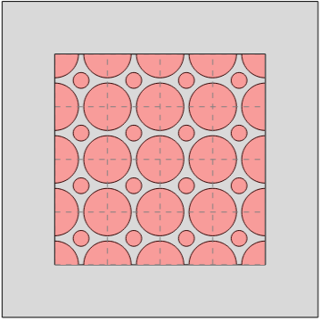
Figure 1: Left: the domain $\Omega$ containing $4\times 4$ SMC unit cells, with $\Omega_{\rm air}$ and $\Omega_{\rm SMC}$ colored in gray and red, respectively; Right: the module $|{\bf u}_{h}|$ of the FE solution ${\bf u}_{h}$ computed with $24\times 24$ SMC unit cells in the domain and with $\sigma_{\rm air}=0.1$. We use $24\times 24$ SMC unit cells for all the computations.

5.1 Two-dimensional example

We first consider a 2D curl-curl problem to test the robustness of our methods for strongly heterogeneous coefficients with high contrast. The problem arises from the eddy current problem in soft magnetic composites (SMCs) [59], which is described by the following equation:

$$\left\{\begin{array}[]{lll}{\displaystyle\nabla\times({\mu}^{-1}\nabla\times{\bf u})+{\sigma}{\bf u}={\bf 0}\,\;\quad{\rm in}\;\,\Omega=[-0.25,1.25]^{2}}\\[5.69054pt] {\displaystyle\;\qquad\qquad\qquad\quad{\bm{n}}\times{\bf u}=1\quad\,\,{\rm on}\;\,\partial\Omega}\end{array}\right.$$

with

$$\mu=\left\{\begin{array}[]{lll}{\displaystyle 50\qquad{\rm in}\;\,\Omega_{\text{SMC}}}\\[5.69054pt] {\displaystyle 1\;\;\qquad{\rm in}\;\,\Omega_{\text{air}}},\end{array}\right.\qquad\text{and}\quad\quad\sigma=\left\{\begin{array}[]{lll}{\displaystyle 100\quad\;\;\quad{\rm in}\;\,\Omega_{\text{SMC}}}\\[5.69054pt] {\displaystyle\sigma_{\text{air}}\;\;\quad\quad{\rm in}\;\,\Omega_{\text{air}}},\end{array}\right.$$

where $\Omega_{\text{SMC}}\subset[0,1]^{2}$ and $\Omega_{\text{air}}=\Omega\setminus\Omega_{\text{SMC}}$ denote the subdomains occupied by the SMC and the air, respectively. The SMC consists of $n\times n$ copies of a scaled unit cell; see Fig.˜1 (left) for an illustration of the domain with $n=4$. We take $n=24$ for all our experiments. The conductivity $\sigma_{\text{air}}$ is chosen as a small positive constant, resulting in a large contrast $100/\sigma_{\rm air}$ in the coefficient $\sigma$. The computational setting is exactly the same as in [59].

The FE discretization is based on a structured triangular mesh with $h=1/800$. Unless otherwise stated, we use the lowest-order Nédélec elements for the discretization, with about $1.9\times 10^{6}$ unknowns in the resulting linear system. The overlapping decomposition $\{\omega_{i}\}$ of the domain $\Omega$ is defined by first partitioning $\Omega$ into $m\times m$ uniform non-overlapping subdomains, and then enlarging each subdomain by adding two layers of adjoining fine mesh elements. Each $\omega_{i}$ is further extended by adding several layers of fine mesh elements to create the corresponding oversampling domain $\omega_{i}^{\ast}$. The number of these additional layers is denoted by ‘Ovsp’, and thus the actual oversampling size is $\text{Ovsp}\times h$. We denote by $n_{\rm loc}$ the number of local eigenvectors used per subdomain for building the coarse space. We use a partition of unity similar to the one described in [40], but with a distance function defined on edges instead of on vertices.

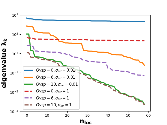
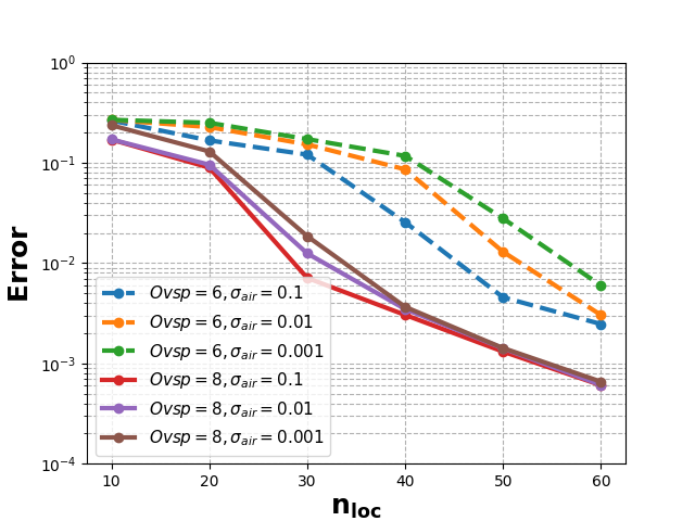
Figure 2: 2D example: the computed eigenvalues of MS-GFEM on an interior subdomain with $m=12$ (left) and the (relative) errors of MS-GFEM with $m=8$ (right).

Figure˜2 (left) plots the computed eigenvalues of MS-GFEM on an interior subdomain with different oversampling sizes. Without oversampling ($\text{Ovsp}=0$), the eigenvalues are nearly constant, but when a small oversampling is used, they decay exponentially as predicted. Moreover, a larger oversampling size yields a faster eigenvalue decay. We also observe that the eigenvalues corresponding to $\sigma_{\rm air}=0.01$ are noticeably larger than those corresponding to $\sigma_{\rm air}=1$ for very small oversampling sizes ($\text{Ovsp}=0$ or 6), but are approximately the same for the size $\text{Ovsp}=10$ (corresponding to an oversampling ratio of 1.28). This shows that the effect of a high coefficient contrast on the eigenvalues can be offset by using a moderate oversampling. Figure˜2 (right) displays the convergence of MS-GFEM with respect to $n_{\rm loc}$ for different choices of Ovsp and $\sigma_{\rm air}$. We see that with $\text{Ovsp}=6$, the errors are noticeably larger for higher coefficient contrasts, but with a slightly larger oversampling size $\text{Ovsp}=8$, they are comparable and are significantly smaller than in the former case. This shows that using a slightly larger oversampling can significantly improve the robustness of the method for coefficient contrasts.

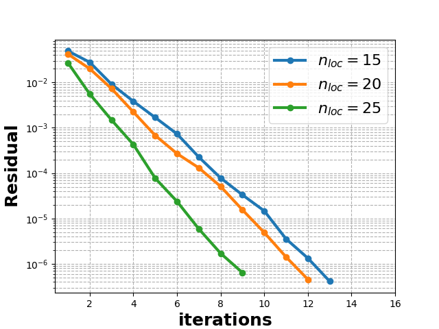
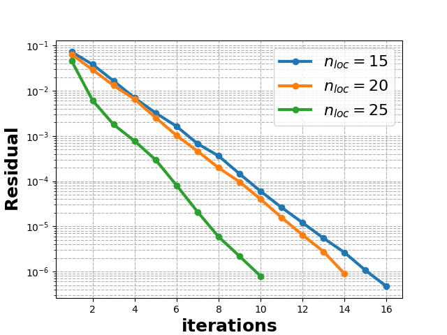
Figure 3: 2D example: the convergence history of the preconditioned GMRES for $\sigma_{\rm air}=1$ (left) and $\sigma_{\rm air}=0.01$ (right) with $m=8$ and $\text{Ovsp}=6$.

$\text{Ovsp}\textbackslash n_{\rm loc}$	10	20	30	40	50	60
2	21 (32)	21 (31)	21 (29)	21 (24)	21 (23)	19 (22)
4	18 (29)	18 (20)	17 (19)	14 (16)	13 (16)	11 (14)
6	16 (18)	15 (17)	11 (15)	9 (12)	8 (9)	3 (4)
8	14 (16)	9 (11)	5 (7)	3 (4)	2 (3)	2 (2)
10	6 (13)	3 (7)	2 (3)	2 (3)	2 (2)	2 (2)

Table 1: 2D example: the iteration counts of GMRES for $\sigma_{\rm air}=0.001$ with $m=8$. The corresponding iteration numbers for the quadratic Nédélec elements are shown in the parentheses.

Figure˜3 depicts the convergence history of GMRES preconditioned with MS-GFEM with different local space sizes $n_{\rm loc}$. We observe that a larger $n_{\rm loc}$ leads to a faster residual reduction as expected. Moreover, there is only a small difference in the iteration counts between $\sigma_{\rm air}=1$ and $\sigma_{\rm air}=0.01$. Notably, the algorithm can converge in 16 iterations with $n_{\rm loc}=15$ and $m=8$ – the size of the coarse problem is as small as 1/2000 of the fine-scale problem. Table˜1 exhibits the iteration counts of the preconditioned GMRES with different oversampling and local space sizes for $\sigma_{\rm air}=0.001$. We observe that with a larger oversampling size, the decrease in the iteration counts with increasing $n_{\rm loc}$ is more significant. Moreover, with reasonably large Ovsp and $n_{\rm loc}$, the algorithm can converge in only two iterations. However, using large oversampling and local space sizes results in significant computational cost, particularly in the solution of the local eigenproblems. In fact, as shown in [63], this is generally not optimal for the overall computational efficiency of the algorithm. We also see from Table˜1 that the algorithm for the quadratic Nédélec elements generally needs more iterations than that for the lowest-order Nédélec elements, but for large local space sizes, the iteration counts are almost the same.

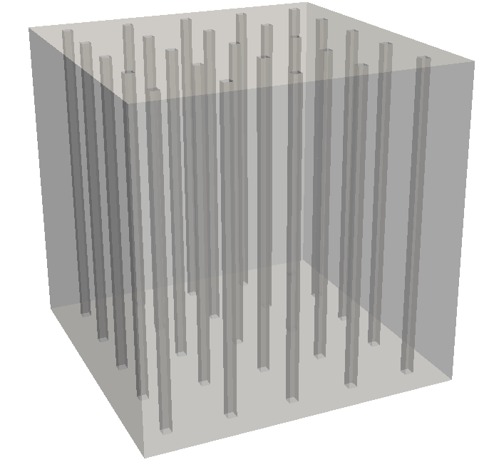
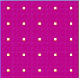
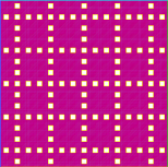
Figure 4: Computational domains with an increasing number of holes that extend along the $z$-direction: 25 (top right), 125 (bottom left), and 225 (bottom right) holes, all shown in the $x$-$y$ plane. The 3D diagram of the domain with 25 holes is shown on the top left.

5.2 Three-dimensional example

In this example, we test the robustness of our methods for domains with non-trivial topologies. We choose the constant coefficients $\kappa=\nu=1$ and the source term ${\bm{f}}=(1,1,1)$ in equation Eq.˜2 for our test. The computational domain $\Omega$ is a unit cube with holes that extend along the $z$-direction of the domain; see Fig.˜4 for three domain configurations. In particular, we refer to the models with holes $25$, $125$, and $225$ as model 1 (‘m1’), model 2 (‘m2’), and model 3 (‘m3’), respectively. The FE discretizations for these models are based on the same structured tetrahedral mesh with $h=1/100$ and on the lowest-order Nédélec elements. The resulting linear systems contain 6165240, 5795140, 5425040 unknowns, respectively.

To implement MS-GFEM, we first partition the computational domain into $250$ uniform non-overlapping subdomains, with $5\times 5$ subdomains in the $xy$-plane and 10 subdomains in the $z$-direction. The numbers of holes in each subdomain in the three models are 1, 5, and 9, respectively. Each subdomain is extended by adding one layer of fine mesh elements to define the overlapping decomposition $\{\omega_{i}\}$. As before, we denote by ‘Ovsp’ the number of layers of fine mesh elements added to each $\omega_{i}$ to create the corresponding oversampling domain $\omega_{i}^{\ast}$, and by $n_{\rm loc}$ the number of local eigenvectors used per subdomain for building the coarse space. We note that due to the presence of holes, the oversampling domains can include boundaries with a "sawtooth" shape. We use the same partition of unity as for the 2D example.

Figure˜5 (left) depicts the computed eigenvalues of MS-GFEM on an interior subdomain for the three models with different oversampling sizes. We observe that for all three models, the eigenvalues decay exponentially with a higher rate for a larger oversampling size, which agrees well with our theoretical predictions. Moreover, with more holes in the subdomain, the corresponding eigenvalues $\lambda_{k}$ are significantly smaller for $k>20$, but with a similar decay rate. Interestingly, the topology of the subdomain significantly affects the first few eigenvalues, as shown in Fig.˜5 (right). In particular, we observe that for the three models, the number of the first eigenvalues that remain nearly constant corresponds to the number of holes in the subdomain $\omega_{i}$. This demonstrates that the eigenvalues of MS-GFEM indeed encode important topological information about the associated subdomain.

Figure 5: 3D example: the computed eigenvalues of MS-GFEM on an interior subdomain for the three models (left) and the first 11 eigenvalues with $\text{Ovsp}=6$ (right).

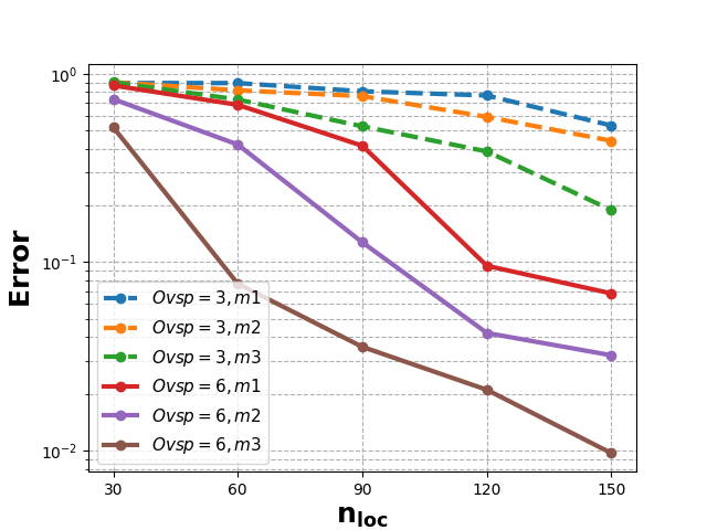
Figure 6: 3D example: the (relative) errors of MS-GFEM.

Figure˜6 displays the convergence of MS-GFEM with increasing local space sizes $n_{\rm loc}$. We observe that as for the 2D example, using a slightly larger oversampling significantly improves the convergence rate of the method. But as predicted by our theory, the convergence rate in 3D is much lower than that in 2D. In addition, the more holes in the domain, the smaller the errors are, which is in line with the behavior of the eigenvalues shown above. Table˜2 gives the iteration counts of the preconditioned GMRES with different local space sizes. We observe that increasing the local space size leads to only a limited decrease in the iteration counts, especially for a very small oversampling size. Although increasing the oversampling and local space sizes can reduce the iteration numbers needed, it also results in a significant growth in computational overhead. In practice, it is often preferable to use small oversampling and local space sizes with a few more iterations. The advantage of the iterative solver is that even with a fairly small coarse space, the method can converge reasonably fast. Indeed, as shown in the table, the method can converge in 34 iterations for all three models with $\text{Ovsp}=2$ and $n_{\rm loc}=20$. With this setting, the size of the coarse problem is only 2500, achieving (at least) a 2170$\times$ reduction in model size.

$n_{\rm loc}$	model 1		model 2		model 3
	$\text{Ovsp}=2$	$\text{Ovsp}=4$	$\text{Ovsp}=2$	$\text{Ovsp}=4$	$\text{Ovsp}=2$	$\text{Ovsp}=4$
20	34	33	33	21	32	23
30	33	21	24	20	20	15
40	30	19	22	18	20	13
50	23	17	22	18	20	13
60	22	16	21	16	20	12
80	21	14	21	13	19	8
100	21	11	20	13	19	6
120	20	12	19	10	15	5

Table 2: 3D example: the iteration counts of GMRES for the three models.

6 Conclusions

We have applied the discrete MS-GFEM as a model reduction technique for discretized $H(\mathrm{curl})$ elliptic problems, and have rigorously established its exponential convergence under minimal assumptions. To address the computational challenge of solving large coarse-scale systems, we further reformulated the discrete MS-GFEM as a two-level restricted additive Schwarz method, with provable convergence guarantees. Numerical experiments demonstrate the effectiveness of the proposed methods in handling problems with highly heterogeneous, high-contrast coefficients and topologically complex domains. Notably, the iterative solver achieves convergence within a small number of iterations, even when the coarse problem size is as small as $1/2000$ of the fine-scale problem. Future work will explore the extension of these techniques to time-harmonic Maxwell’s equations, by combining the methodology presented in this paper with the preconditioning strategy introduced in [14].

References

- [1] R. Altmann, P. Henning, and D. Peterseim, Numerical homogenization beyond scale separation, Acta Numer., 30 (2021), pp. 1–86.
- [2] C. Amrouche and I. Boussetouan, Vector potentials with mixed boundary conditions. Application to the Stokes problem with pressure and Navier-type boundary conditions, SIAM J. Math. Anal., 53 (2021), pp. 1745–1784.
- [3] R. Araya, C. Harder, D. Paredes, and F. Valentin, Multiscale hybrid-mixed method, SIAM Journal on Numerical Analysis, 51 (2013), pp. 3505–3531.
- [4] D. Arnold, R. Falk, and R. Winther, Finite element exterior calculus: from Hodge theory to numerical stability, Bull. Amer. Math. Soc., 47 (2010), pp. 281–354.
- [5] D. N. Arnold, Finite element exterior calculus, SIAM, 2018.
- [6] D. N. Arnold, R. S. Falk, and R. Winther, Finite element exterior calculus, homological techniques, and applications, Acta Numer., 15 (2006), pp. 1–155.
- [7] I. Babuska and R. Lipton, Optimal local approximation spaces for generalized finite element methods with application to multiscale problems, Multiscale Model. Simul., 9 (2011), pp. 373–406.
- [8] A. Bensoussan, J.-L. Lions, and G. Papanicolaou, Asymptotic analysis for periodic structures, vol. 374, American Mathematical Soc., 2011.
- [9] M. Bergot and P. Lacoste, Generation of higher-order polynomial basis of Nédélec H(curl) finite elements for Maxwell’s equations, J. Comput. Appl. Math., 234 (2010), pp. 1937–1944.
- [10] D. Boffi, F. Brezzi, and M. Fortin, Mixed finite element methods and applications, vol. 44, Springer, 2013.
- [11] N. Bootland, V. Dolean, F. Nataf, and P.-H. Tournier, A robust and adaptive geneo-type domain decomposition preconditioner for H(curl) problems in three-dimensional general topologies, arXiv preprint arXiv:2311.18783, (2023).
- [12] J. Calvo, A bddc algorithm with deluxe scaling for H(curl) in two dimensions with irregular subdomains, Math. Comp., 85 (2016), pp. 1085–1111.
- [13] L. Cao, Y. Zhang, W. Allegretto, and Y. Lin, Multiscale asymptotic method for Maxwell’s equations in composite materials, SIAM J. Numer. Anal., 47 (2010), pp. 4257–4289.
- [14] Z. Chen, L. Wang, and W. Zheng, An adaptive multilevel method for time-harmonic Maxwell equations with singularities, SIAM J. Sci. Comput., 29 (2007), pp. 118–138.
- [15] E. Chung, Y. Efendiev, and T. Y. Hou, Multiscale Model Reduction, Springer, 2023.
- [16] E. T. Chung, Y. Efendiev, and W. T. Leung, Constraint energy minimizing generalized multiscale finite element method, Comput. Methods. Appl. Mech. Eng., 339 (2018), pp. 298–319.
- [17] E. T. Chung and Y. Li, Adaptive generalized multiscale finite element methods for H(curl)-elliptic problems with heterogeneous coefficients, J. Comput. Appl. Math., 345 (2019), pp. 357–373.
- [18] C. R. Dohrmann and O. B. Widlund, An iterative substructuring algorithm for two-dimensional problems in H(curl), SIAM J. Numer. Anal., 50 (2012), pp. 1004–1028.
- [19] V. Dolean, F. Nataf, R. Scheichl, and N. Spillane, Analysis of a two-level Schwarz method with coarse spaces based on local Dirichlet-to-Neumann maps, Comput. Methods Appl. Math., 12 (2012), pp. 391–414.
- [20] W. E and B. Engquist, The heterognous multiscale methods, Commun. Math. Sci., 1 (2003), pp. 87–132.
- [21] Y. Efendiev, J. Galvis, and T. Y. Hou, Generalized multiscale finite element methods (GMsFEM), J. Comput. Phys., 251 (2013), pp. 116–135.
- [22] M. Faustmann, J. M. Melenk, and M. Parvizi, H-matrix approximability of inverses of FEM matrices for the time-harmonic Maxwell equations, Adv. Comput. Math., 48 (2022), p. 59.
- [23] D. Gallistl, P. Henning, and B. Verfürth, Numerical homogenization of H(curl)-problems, SIAM J. Numer. Anal., 56 (2018), pp. 1570–1596.
- [24] J. Galvis and Y. Efendiev, Domain decomposition preconditioners for multiscale flows in high-contrast media, Multiscale Model. Simul., 8 (2010), pp. 1461–1483.
- [25] V. Gol’dshtein, I. Mitrea, and M. Mitrea, Hodge decompositions with mixed boundary conditions and applications to partial differential equations on Lipschitz manifolds., J. Math. Sci., 172 (2011).
- [26] M. Hauck and D. Peterseim, Super-localization of elliptic multiscale problems, Math. Comp., 92 (2023), pp. 981–1003.
- [27] F. Hecht, New development in FreeFem++, J. Numer. Math., 20 (2012), pp. 251–266.
- [28] A. Heinlein, A. Klawonn, J. Knepper, and O. Rheinbach, Adaptive GDSW coarse spaces for overlapping Schwarz methods in three dimensions, SIAM J. Sci. Comput., 41 (2019), pp. A3045–A3072.
- [29] P. Henning, M. Ohlberger, and B. Verfürth, A new heterogeneous multiscale method for time-harmonic Maxwell’s equations, SIAM J. Numer. Anal., 54 (2016), pp. 3493–3522.
- [30] P. Henning and A. Persson, Computational homogenization of time-harmonic Maxwell’s equations, SIAM J. Sci. Comput., 42 (2020), pp. B581–B607.
- [31] R. Hiptmair and C. Pechstein, Discrete regular decompositions of tetrahedral discrete 1-forms, Maxwell’s equations—analysis and numerics, 24 (2019), pp. 199–258.
- [32] R. Hiptmair and C. Pechstein, A review of regular decompositions of vector fields: continuous, discrete, and structure-preserving, Spectral and High Order Methods for Partial Differential Equations, (2020), p. 45.
- [33] R. Hiptmair and A. Toselli, Overlapping and multilevel Schwarz methods for vector valued elliptic problems in three dimensions, in Parallel solution of partial differential equations, Springer, 2000, pp. 181–208.
- [34] R. Hiptmair and J. Xu, Nodal auxiliary space preconditioning in H(curl) and H(div) spaces, SIAM J. Numer. Anal., 45 (2007), pp. 2483–2509.
- [35] M. Hochbruck, B. Maier, and C. Stohrer, Heterogeneous multiscale method for Maxwell’s equations, Multiscale Model. Simul., 17 (2019), pp. 1147–1171.
- [36] T. Y. Hou and X.-H. Wu, A multiscale finite element method for elliptic problems in composite materials and porous media, J. Comput. Phys., 134 (1997), pp. 169–189.
- [37] Q. Hu, Convergence of the Hiptmair–Xu preconditioner for Maxwell’s equations with jump coefficients (i): Extensions of the regular decomposition, SIAM J. Numer. Anal., 59 (2021), pp. 2500–2535.
- [38] Q. Hu, Convergence of the Hiptmair–Xu preconditioner for H(curl)-elliptic problems with jump coefficients (ii): Main results, SIAM J. Numer. Anal., 61 (2023), pp. 2434–2459.
- [39] Q. Hu and J. Zou, A nonoverlapping domain decomposition method for Maxwell’s equations in three dimensions, SIAM J. Numer. Anal., 41 (2003), pp. 1682–1708.
- [40] P. Jolivet, F. Hecht, F. Nataf, and C. Prud’Homme, Overlapping domain decomposition methods with FreeFem++, in Domain Decomposition Methods in Science and Engineering XXI, Springer, 2014, pp. 315–322.
- [41] T. V. Kolev and P. S. Vassilevski, Parallel auxiliary space AMG for H(curl) problems, J. Comput. Math., (2009), pp. 604–623.
- [42] G. Kristensson and N. Wellander, Homogenization of the Maxwell equations at fixed frequency, SIAM J. Appl. Math., 64 (2003), pp. 170–195.
- [43] Q. Liang, X. Xu, and S. Zhang, On a sharp estimate of overlapping Schwarz methods in H(curl; ) and H(div; ), IMA J. Numer. Anal., (2024), p. drae022.
- [44] M. Licht, Smoothed projections and mixed boundary conditions, Math. Comp., 88 (2019), pp. 607–635.
- [45] C. Ma, A unified framework for multiscale spectral generalized FEMs and low-rank approximations to multiscale PDEs, Found. Comput. Math., (2025), pp. 1–60.
- [46] C. Ma, C. Alber, and R. Scheichl, Wavenumber explicit convergence of a multiscale generalized finite element method for heterogeneous Helmholtz problems, SIAM J. Numer. Anal., 61 (2023), pp. 1546–1584.
- [47] C. Ma and J. M. Melenk, Exponential convergence of a generalized FEM for heterogeneous reaction-diffusion equations, Multiscale Model. Simul., 22 (2024), pp. 256–282.
- [48] C. Ma and R. Scheichl, Error estimates for discrete generalized FEMs with locally optimal spectral approximations, Math. Comp., 91 (2022), pp. 2539–2569.
- [49] C. Ma, R. Scheichl, and T. Dodwell, Novel design and analysis of generalized finite element methods based on locally optimal spectral approximations, SIAM J. Numer. Anal., 60 (2022), pp. 244–273.
- [50] A. Målqvist and D. Peterseim, Localization of elliptic multiscale problems, Math. Comp., 83 (2014), pp. 2583–2603.
- [51] A. Målqvist and D. Peterseim, Numerical homogenization by localized orthogonal decomposition, SIAM, 2020.
- [52] J. M. Melenk, On generalized finite element methods. Ph.D. thesis, Department of Mathematics, University of Maryland, 1995.
- [53] P. Monk, Finite element methods for Maxwell’s equations, Oxford university press, 2003.
- [54] D.-S. Oh and S. Zhang, New analysis of overlapping Schwarz methods for vector field problems in three dimensions with generally shaped domains, arXiv preprint arXiv:2404.11986, (2024).
- [55] H. Owhadi, Bayesian numerical homogenization, Multiscale Model. Simul., 13 (2015), pp. 812–828.
- [56] H. Owhadi and C. Scovel, Operator-Adapted Wavelets, Fast Solvers, and Numerical Homogenization: From a Game Theoretic Approach to Numerical Approximation and Algorithm Design, vol. 35, Cambridge University Press, 2019.
- [57] J. E. Pasciak and J. Zhao, Overlapping Schwarz methods in H(curl) on polyhedral domains, J. Numer. Math., 10 (2002), pp. 221–234.
- [58] A. Pinkus, n-widths in Approximation Theory, Springer-Verlag, Berlin, 1985.
- [59] X. Ren, A. Hannukainen, and A. Belahcen, Homogenization of multiscale eddy current problem by localized orthogonal decomposition method, IEEE Trans. Magn., 55 (2019), pp. 1–4.
- [60] Y. Shao, Z. Peng, and J.-F. Lee, Full-wave real-life 3-d package signal integrity analysis using nonconformal domain decomposition method, IEEE Trans. Microwave Theory Techn., 59 (2010), pp. 230–241.
- [61] E. H. Spanier, Algebraic topology, Springer Science & Business Media, 1989.
- [62] N. Spillane, V. Dolean, P. Hauret, F. Nataf, C. Pechstein, and R. Scheichl, Abstract robust coarse spaces for systems of pdes via generalized eigenproblems in the overlaps, Numer. Math., 126 (2014), pp. 741–770.
- [63] A. Strehlow, C. Ma, and R. Scheichl, Fast-convergent two-level restricted additive Schwarz methods based on optimal local approximation spaces, arXiv preprint arXiv:2408.16282, (2024).
- [64] J. M. Tang, R. Nabben, C. Vuik, and Y. A. Erlangga, Comparison of two-level preconditioners derived from deflation, domain decomposition and multigrid methods, J. Sci. Comput., 39 (2009), pp. 340–370.
- [65] A. Toselli, Overlapping Schwarz methods for Maxwell’s equations in three dimensions, Numer. Math., 86 (2000), pp. 733–752.
- [66] A. Toselli, Dual-primal FETI algorithms for edge finite-element approximations in 3D, IMA J. Numer. Anal., 26 (2006), pp. 96–130.
- [67] A. Toselli and O. Widlund, Domain decomposition methods-algorithms and theory, vol. 34, Springer Science & Business Media, 2004.
- [68] P.-H. Tournier, P. Jolivet, and F. Nataf, FFDDM: Freefem domain decomposition method. https://doc.freefem.org/documentation/ffddm/index.html, 2019.
- [69] B. Verfürth, Heterogeneous multiscale method for the Maxwell equations with high contrast, ESAIM Math. Model. Numer. Anal., 53 (2019), pp. 35–61.