Experimental memory control in continuous variable
optical quantum reservoir computing

Abstract

Quantum reservoir computing (QRC) offers a promising framework for online quantum-enhanced machine learning tailored to temporal tasks, yet practical implementations with native memory capabilities remain limited. Here, we demonstrate an optical QRC platform based on deterministically generated multimode squeezed states, exploiting both spectral and temporal multiplexing in a fully continuous-variable (CV) setting, and enabling controlled fading memory. Data is encoded via programmable phase shaping of the pump in an optical parametric process and retrieved through mode-selective homodyne detection. Real-time memory is achieved through feedback using electro-optic phase modulation, while long-term dependencies are achieved via spatial multiplexing. This architecture with minimal post-processing performs nonlinear temporal tasks, including parity checking and chaotic signal forecasting, with results corroborated by a high-fidelity Digital Twin. We show that leveraging the entangled multimode structure significantly enhances the expressivity and memory capacity of the quantum reservoir. This work establishes a scalable photonic platform for quantum machine learning, operating in CV encoding and supporting practical quantum-enhanced information processing.

I Introduction

Reservoir computing is a machine learning neuroinspired paradigm that exploits the dynamics of an artificial network with minimal learning requirements. Unlike other neural network paradigms, in fact, it avoids the computationally intensive process of adjusting internal connection weights during training; only the output layer weights are modified, typically through simple linear regression [1, 2]. While the term reservoir computing is nowadays often used in a broad sense to refer to learning tasks based on an untrained network (i.e. a reservoir), its most distinctive feature is the ability to learn from temporal series (e.g., predicting chaotic time series) by exploiting the memory features of the system used as a reservoir. This internal memory allows to boost the performance in on-line learning, going beyond static tasks (e.g., classification problems, not requiring memory as in Extreme Learning Machines [3, 4]).

Quantum reservoir computing (QRC) expands the physical realm of reservoirs into the quantum regime and has recently been extensively explored theoretically in several platforms [5, 6, 7, 8] where novel capabilities [9, 10, 11, 12], but also challenges emerge [13, 14]. Photonic platforms are particularly appealing, inheriting capabilities in the classical regime [15], and due to the many degrees of freedom that can be exploited, their potential for integration, and, when the information is encoded in the quadrature continuous variables, the possibility to work at room-temperature exploiting coherent detection [16, 7]. Although seminal results have been demonstrated on quantum optical platforms, they have primarily focused on classification tasks [17, 18, 10, 19, 20], or classically assisted strategies [21]. Only very recently have efforts been made to provide memory capabilities within general quantum platforms such as superconducting circuits [22, 23, 24], and in a memristor photonic platform [25].

In this work, we present an experimental realization of memory-tailored quantum reservoir computing by dynamically controlling a multimode quantum network through feedback conditioned on its history. Our approach establishes multimode quantum states multiplexed in both the optical frequency and time-bin degrees of freedom [26, 27, 28] for temporal learning tasks via a continuous-variable quantum reservoir platform and building on theoretical results that show the potential of such systems in QRC [29, 16, 30, 31]. The experimental realization exploits deterministically generated and reconfigurable multimode squeezed and entangled states along with reconfigurable mode-selective homodyne detection. It supports controllable memory demonstrating a performance boost in n-line learning and does not require post-processing with a classical neural network platform.

Data encoding is implemented by controlling either the global phase or the complex spectral shape of the pump pulses in the optical parametric process that generates the multimode quantum resource. When controlling the global phase, the signal is encoded in the angle of the squeezing ellipses of the squeezed spectral modes, effectively modifying the quantum correlations in a given measurement basis. Alternatively, controlling the phase and amplitude of the spectral components of the pump directly alters the quantum correlations among the output spectral components of the quantum signal by modifying the nonlinear optical process. Moreover, we construct a digital twin of the experiment by integrating accurate models of the quantum and nonlinear optical processes, along with the continuous-variable dynamics of the reservoir. This allows for predictive simulations which, when calibrated with a noise model, closely match experimental results and can be used to explore the system’s broader capabilities.

We perform experimental temporal tasks enabled by memory using global phase encoding. Memory is achieved via a feedback signal applied to the electro-optic phase modulator [32] that controls the pump phase; the feedback is derived from observables measured via mode-selective homodyne detection on the multispectral components of the quantum reservoir. For short-memory tasks, we implement real-time feedback control, while longer-delay target functions are experimentally realized using a spatial multiplexing strategy, i.e., by running sequential experiments that act as spatially distributed copies of the quantum reservoir platform. Finally, we demonstrate that exploiting the entangled multimode nature of the system for encoding yields better scaling of reservoir expressivity when compared to the use of multiple independent copies of the experiment (spatial multiplexing).

This demonstrates online temporal processing boosted by a controllable memory for temporal tasks using an entangled squeezed vacuum reservoir. The use of Gaussian states and homodyne detection has already been theoretically shown to enhance information processing capacity compared to classical encodings [29] allowing the saturation of a polynomial advantage, as measured by this capacity in reservoirs of increasing size [16]. This is the regime experimentally explored for the first time in this article, with potential relevance for practical NISQ implementations. Moreover, measurement based techniques with cluster states [31] and relevant non-Gaussian resources [33] can be easily integrated into the same platform.

While defining a quantum advantage in QRC, or more generally in quantum machine learning protocols, remains an open question [34], the general framework of continuous-variable (CV) encoding, particularly when augmented with non-Gaussian resources, is actively pursued for fault-tolerant photonic quantum computing [35]. Our demonstration of online temporal tasks boosted by memory opens the way to scalable quantum reservoir computing, as it requires only the deterministic generation of Gaussian states and deterministic room-temperature detection (e.g., homodyne), to explore quantum advantage, through non-Gaussian resources [36, 37, 38, 39].

II Results

II.1 The quantum resource

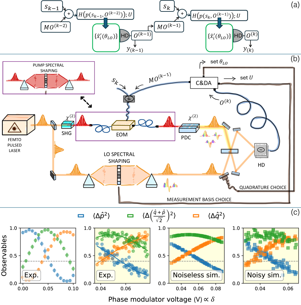
Figure 1: (a) Quantum reservoir protocol. At each time step $k$, the input $s_{k}$ is added to a feedback signal derived from the previous observables $O^{(k-1)}$. This sets the pump of the parametric process, determining the operators $\hat{x}^{\prime}_{i}$ and their quantum correlations. The task output $y_{k}$ is obtained from the observables. (b) Experimental setup. Information is encoded in the global phase of the pump, generated via second harmonic generation (SHG) and modulated by an electro-optic modulator (EOM). The more general encoding involve amplitude and phase shaping of the pump spectrum. The multimode entangled state from parametric down-conversion (PDC), and thus its observables, is tailored by this encoding. The control and data acquisition (C&DA) module includes electronics to set the measurement basis ($U$) via local oscillator shaping in homodyne detection (HD), measure the observables $O_{m}$, and generate the feedback. Phase locking is not shown. (c) Nonlinear dependence of observables with the EOM voltage (proportional to the encoding phase $\delta$). Left: experimental data in low- and average-noise regimes. Right: simulated data using the Digital Twin model according to the experimental noise evaluation. The white panel spans a voltage range sufficient for observables to vary from 0 to 1 (phase difference slightly exceeding $\pi/2$). Yellow panels show observables recorded during training on a memory task.

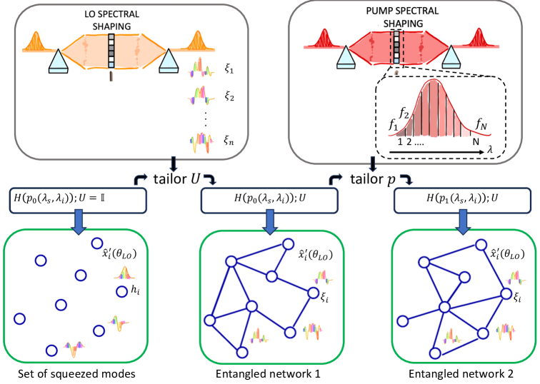
Figure 2: Controllability of the resource by tailoring the local oscillator spectral shape and the pump spectral. The nodes of the network are different spectro-temporal modes of the field. The set of modes are defined by the basis choice $U$. For convention when $U=I$ the supermode basis $\{h_{i}\}$ is chosen, and the modes are independently squeezed. In all the other mode basis $\{\xi_{i}\}$ the modes show entanglement correlations represented as links in a network. The general mode quadrature is $\hat{x}^{\prime}_{i}(\theta_{LO})=\cos{(\theta_{LO})}\hat{q}_{i}^{\prime}+\sin{(\theta_{LO})}\hat{p}_{i}^{\prime}$ that corresponds to $\hat{q}_{i}^{\prime}$ or $\hat{p}_{i}^{\prime}$ if the local oscillator phase is set to be $\theta_{LO}=0$ or $\theta_{LO}=\pi/2$. The correlations can be controlled by tailoring the pump of the process that modifies the Hamiltonian.

The core of the quantum resource is a multimode optical network generated via parametric down conversion in a non-linear waveguide pumped by a pulsed laser, as shown as in Fig. 1. The interaction Hamiltonian of the process generating the couple of signal and idler fields of wavelengths $\lambda_{S},\lambda_{I}$ reads

$$\hat{H}\propto\int d\lambda_{S}d\lambda_{I}\,J(\lambda_{S},\lambda_{I})\,\hat{a}^{\dagger}(\lambda_{S})\hat{b}^{\dagger}(\lambda_{I})+\text{h.c.}$$ (1)

where $J(\lambda_{S},\lambda_{I})$ is the so called joint spectral amplitude (JSA) which can be written as [40, 41, 42]:

$$J(\lambda_{S},\lambda_{I})=p(\lambda_{S},\lambda_{I})\cdot\phi(\lambda_{S},\lambda_{I})$$ (2)

The term $p(\lambda_{S},\lambda_{I})$ is the complex pump spectral shape, while $\phi(\lambda_{S},\lambda_{I})$ is the phase-matching function, determined by the characteristics of the nonlinear medium. The multimode nature of the generated quantum system can be retrieved by performing a Schmidt decomposition of the JSA $J(\lambda_{S},\lambda_{I})=\sum_{k}r_{k}h_{k}(\lambda_{S})g_{k}(\lambda_{I})$, where $h_{k}(\lambda_{S})$ and $g_{k}(\lambda_{I})$ are two sets of orthonormal modes, spectral profiles of signal and idler channels, and $r_{k}$ are called the Schmidt coefficients. In case of degenerate signal and idler fields, as in our experimental setup, $h_{k}=g_{k};$ and the Hamiltonian in Eq.(1) can be written as $\hat{H}\propto\sum_{k}r_{k}\,\hat{A}_{k}^{\dagger 2}+\text{h.c.}$, with $\hat{A}_{k}^{\dagger}$ broadband creation operators associated to the modes $h_{k}$. When acting on an initial vacuum field, the latter Hamiltonian generates a tensor product of single-mode squeezed vacuum states, one in each mode $h_{k}(\lambda_{S})$, that are also called supermodes. The number of non-zero $r_{k}$ terms tells the minimal number of modes that are necessary to describe the quantum features of the generated signal. This number and the spectral shape of the corresponding modes is determined by the JSA. For a pump with large enough Gaussian spectrum the supermodes $h_{k}(\lambda_{S})$ are described by Hermite-Gauss polynomials, as shown at the output of the parametric process in Fig. 1. The used setup can generate up to 40 Schmidt modes (see Appendix for more information).

The produced quantum state is Gaussian and can be fully described in phase-space by the covariance matrix $\boldsymbol{\sigma}$ of its quadratures, measured via homodyne detection. The elements of the covariance matrix are $\sigma_{ij}=1/2\langle\Delta\hat{x}_{i}\Delta\hat{x}_{j}+\Delta\hat{x}_{j}\Delta\hat{x}_{i}\rangle$, being $\Delta\hat{x}_{i}=\hat{x}_{i}-\langle\hat{x}_{i}\rangle$ and $\hat{x}_{i}$ the quadrature $\hat{q}_{i}$ or $\hat{p}_{i}$ of the mode $i$ with commutation relation $[\hat{q}_{i},\hat{p}_{i}]=2\imath$. The covariance matrix is obtained via the symplectic transformation governed by the interaction Hamiltonian and in the basis of supermodes it takes the form of a diagonal matrix $\boldsymbol{\sigma}(H)=\text{diag}\{e^{2r_{1}},e^{2r_{2}},...,e^{-2r_{1}},e^{-2r_{2}},...\}$. A mode-selective homodyne detection allows us to probe the quantum state in a specific mode basis. If, instead of measuring the supermodes, we perform measurements in another orthonormal mode basis $\{\xi_{j}(\lambda_{S})\}$, linked to the supermodes via the unitary transformation $\boldsymbol{U}$, the covariance matrix in the new basis becomes $\boldsymbol{\sigma}^{\prime}=\boldsymbol{S_{U}}^{T}\,\boldsymbol{\sigma}\,\boldsymbol{S_{U}}$ with $\boldsymbol{S_{U}}$, a symplectic transformation driven by $\boldsymbol{U}$ (see the Appendix for details).

The matrix $\boldsymbol{\sigma}^{\prime}$ is now non-diagonal and the off-diagonal terms are signatures of entanglement correlations between the measured modes. Measuring on such basis allows to experimentally access entanglement correlations for quantum protocols [43, 28]. The resource can then be pictured via an entangled network as shown in Fig. 2.

Once the experiment is settled, the phase-matching function term of the JSA in Eq.(2) is fixed by the material and waveguide properties and only the pump-envelope function can be modified in a reconfigurable way via mode-shaping techniques. This modifies the entanglement correlation between nodes as shown in Fig. 2. Therefore, we can explicitly write the dependence of the covariance matrix $\boldsymbol{\sigma}^{\prime}$ on the pump $p$ and the chosen basis $U$ as $\boldsymbol{\sigma}^{\prime}=\boldsymbol{S_{U}}^{T}\,\boldsymbol{\sigma(H(p))}\,\boldsymbol{S_{U}}$.

In the following we exploit the control on the pump-envelope function to encode information in the quantum system in the configuration of a fixed measurement basis $U$. The expectation value of general observables $O_{m}=\langle\Delta\hat{x}_{i}\Delta\hat{x}_{j}\rangle$ that will be used in the reservoir task, can be retrieved from the covariance matrix $\boldsymbol{\sigma}^{\prime}(U,p)$. Given the pump shape, we have accurate numerical models of the process from the non-linear interaction to the observables [40, 41, 42], which allows us to set a Digital Twin of the experimental setup as fully explained in Appendix.

II.2 Information encoding and memory control of the quantum reservoir

When we tune the pump phase profile, the pump-envelope function can be written as:

$$p(\lambda_{P},\boldsymbol{\delta})=\sum_{i=1}^{N}f_{i}(\lambda_{P})e^{i\delta_{i}}$$ (3)

where the $f_{i}(\lambda_{P})$, with $\lambda_{P}=(1/\lambda_{S}+1/\lambda_{I})^{-1}$, are a set of $N$ pump modes, and the $\boldsymbol{\delta}=(\delta_{i})_{i=1}^{N}\in\mathbb{R}^{N}$ are tunable phase parameters that allow precise shaping of the JSA to easily encode information. The pump input modes $f_{i}$ that we consider are $N$ frequency windows, delimiting a portion of our Gaussian pump profile $f(\lambda_{P})$, that we can precisely control with a spatial light modulator. To perform the measurement, a set of $n$ modes $\xi_{j}(\lambda_{S})$ is selected by the basis choice $U$ via the local oscillator shaping in homodyne (see Subsec. IV.3). The tailoring of $N$ pump spectral components and the choice of the measurement basis composed by $n$ elements are shown in the upper part of Fig. 2. More details about the input and output modes used are in Subsec. IV.3.

Our system is endowed with memory through a real-time feedback mechanism: the results of previous measurements are fed back into the system to influence future states. Specifically, if we consider a discrete-time sequence of inputs $\{s_{k}\}$, where $k$ denotes the timestep, the pump parameters are updated according to:

$$\delta_{i}^{(k)}=\alpha_{i}s_{k}+\beta_{i}+\sum_{m}M_{im}O_{m}^{(k-1)}$$ (4)

Here, $i\in 1,...,N$, $\alpha_{i}$ and $\beta_{i}$ are real-valued coefficients, and $M_{im}$ is a feedback mask (a real matrix) that determines how previous measurement outcomes influence the current pump parameters. This determines the fading memory of the QRC. The quantities $O_{m}^{(k-1)}=\langle\Delta\hat{x}_{i}\Delta\hat{x}_{j}\rangle^{(k-1)}$ are the values of the $m^{\text{th}}$ observable measured at timestep $k-1$, and are derived from a subset of the elements of the covariance matrix ($i,j\in 1,\dots,2n$). These are measured by accumulating data on the homodyne signal. So the reservoir computing is described by the following:

$$\begin{cases}O_{m}^{(k)}\propto\sigma^{\prime(k)}_{ij}\mid\boldsymbol{\sigma}^{\prime(k)}=\boldsymbol{S_{U}}^{T}\,\boldsymbol{\sigma(H(p(s_{k},\boldsymbol{O}^{(k-1)})))}\,\boldsymbol{S_{U}}\\ y_{k}=\mathbf{w}^{T}\mathbf{O}^{(k)}+b\par\end{cases}$$ (5)

The reservoir is trained by adjusting the matrix $\mathbf{w}$ and parameter $b$ to minimize the error in the chosen learning task. The scheme of the quantum reservoir with feedback is shown in the top part of Fig. 1. While we here focus on the case of feedback restricted to the last output at each cycle, the fading memory can be extended re-injecting a longer combination of past signals.

The case $N>1$ allows to encode vector inputs $\vec{s}_{k}$, where $\text{dim}_{\text{vec}}(\vec{s}_{k})\leq N$, by distributing the elements of $\vec{s}_{k}$ on the different phases $\delta_{i}$. A particular case of encoding corresponds to choosing $N=1$. In this case, we encode information on the global phase of the pump. This has been experimentally implemented by modulating the pump phase via an electro-optic modulator (EOM), as shown in Fig. 1.

II.3 Quantum reservoir computing tasks

We evaluate the performance of our system across a range of benchmark tasks using two types of input encoding: the simple, experimentally implemented scheme with $N=1$, and the more general encoding with $N>1$. We begin with the XOR task, which assesses the system’s ability to capture nonlinearity and short-term memory while requiring minimal resources. We then consider the memory task to characterize the system’s fading memory property. Finally, we turn to more complex benchmarks, including the double-scroll and parity check tasks, which challenge the system’s scalability and its capacity to handle richer, higher-order nonlinear dynamics.

II.3.1 Experimental control of memory via global phase

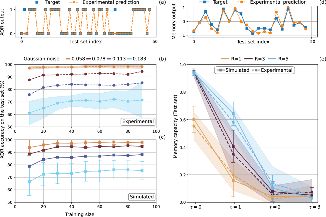
Figure 3: XOR task (experimental and simulated). (a) Example of binary target (blue) and predicted (orange) outputs for the test set, with a test accuracy of $95.9\%$ (correct predictions over total). Training and test sizes are 99 and 49, respectively. (b,c) Test accuracy versus training size: experimental (dots) and simulated (squares) results under varying noise levels (light brown, brown, blue, light blue). Experimental error bars (shaded) are obtained by reshuffling data before the train/test split; simulated ones from repeated sampling. Larger training sets lead to smaller test sets, increasing variability due to single misclassifications. For clarity, error bars are shown only for the first and last noise levels. Memory task (experimental and simulated). (d) Continuous target (blue) and predicted (orange) output for a test set using $5$ reservoirs with delay $\tau=1$ (capacity $=0.81$). (e) Capacities vs. delay $\tau$: experimental (dots) and simulated (squares) results for different reservoir numbers (light brown, dark purple, light blue). Error bars are computed as for the XOR task. In both cases, simulations use a realistic experimental noise model via the Digital Twin.

The phase encoding via the electro-optic modulator corresponds to the case of $N=1$, where the voltage applied changes linearly the pump phase $\delta$ (see Appendix):

$$p(\lambda_{P},\delta)=f(\lambda_{P})e^{i\delta}$$ (6)

where $f(\lambda_{P})$ is the natural Gaussian profile of the pump. As later shown in Subsec. II.3.2, with this type of encoding, the expressivity of the observables does not significantly increase with the number of measured modes $n$, therefore we use $n=1$ as well. This means that we directly measure by selecting the first supermode $h_{1}$ and we use as observables $\{O_{1},O_{2},O_{3}\}$ the set $\{\langle\Delta\hat{q}^{2}\rangle$, $\langle\Delta\hat{p}^{2}\rangle,$ $\langle\Delta\hat{q}\Delta\hat{p}\rangle\sim\langle\Delta(\frac{\hat{q}+\hat{p}}{\sqrt{2}})^{2}\rangle\}$, where we removed the mode index $1$ from the quadrature operators. These three observables are sufficient for implementing several tasks, as they express three different dependencies with respect to $\delta$ as shown in the lower part of Fig. 1. For linear regressions indeed, observables that are correlated (linearly dependent) are redundant (see [44, 45] and for more qualitative details Sec. IV). For example, measuring $\langle\Delta(\frac{\hat{q}+\hat{p}}{\sqrt{2}})^{2}\rangle$ is equivalent to measuring $\langle\Delta\hat{q}\Delta\hat{p}\rangle$ since analytically, for a global phase encoding, $\langle\Delta\hat{q}\Delta\hat{p}\rangle(\delta)=\langle\Delta(\frac{\hat{q}+\hat{p}}{\sqrt{2}})^{2}\rangle(\delta)+cst$ (as shown in the Appendix). In the bottom of Fig. 1 the first two panels show the experimental dependence of the three observables on $\delta$, encoded via the voltage of the phase modulator, in the case of a low-noise realization and a more noisy one, which is representative of the average noise in measurements. Assuming a Gaussian noise model, the typical variance of observables is recovered via a Least Square method (see the Appendix ). The result is used in the Digital Twin to simulate the expected behavior as shown in the last two panels.

The unique non-zero term $M$ we use for the feedback mask is the one corresponding to $\langle\Delta\hat{q}^{2}\rangle^{(k-1)}$. At each timestep $k$, we set the global phase depending on the input $s_{k}$ and the feedback as:

$$\delta^{(k)}=\alpha s_{k}+\beta+M\langle\Delta\hat{q}^{2}\rangle^{(k-1)}$$ (7)

$M$, $\alpha$ and $\beta$ are randomly chosen within ranges that ensure both the input and the feedback contribute comparably to the phase. These ranges are selected to explore a nontrivial region of the observable space (see Subsec. IV.7 for more details).

We begin with a binary task, the temporal XOR, where the target output is $\hat{y}_{k}=s_{k}\bigoplus s_{k-1}$ and the input is a sequence of binary values $s_{k}\in\{0,1\}$. This task requires both nonlinearity as well as memory of the previous encoded input at each timestep. The reservoir is trained on a set of inputs using linear regression applied to the measured observables. The goal is to determine the optimal weights $\mathbf{w},b$ that maximize accuracy (see Sec. IV) by matching the predicted outputs $y_{k}$ (we put a threshold at $0.5$ to divide into $0$s and $1$s) with the known targets $\hat{y}_{k}$ in the training set.

The performance of the reservoir is then evaluated using the accuracy again, but on a test sequence of new data. In plot (a) of Fig. 3, we present an example of the test target values and the corresponding experimental prediction. In plots (b) and (c) below, we show experimental and simulated accuracies as a function of training set size, for different levels of Gaussian noise. Experimental instabilities can introduce Gaussian noise in the measurement of the observables (see Fig. 1), which can be mitigated by averaging over repeated measurements. These instabilities arise from mechanical and thermal fluctuations and are not intrinsic limitations of the protocol, but rather reflect the current performance of the experimental setup. We see that the training saturates for set sizes around 100 and that noise affects the performance. Nevertheless, the reservoir could achieve experimentally test accuracies of $98\pm 1\%$ for realistic levels of noise, with only $70$ training steps. The experimental noise is also well numerically simulated with a Gaussian model and the results are similar, as shown in plot (c) of Fig. 3.

A way to further test the memory of the system is through the linear memory task, in which the reservoir is trained to reproduce past entries of the input series. The target function at timestep $k$ is the input encoded $\tau$ steps in the past, $\hat{y}_{k}=s_{k-\tau}$. For the input, we generate a sequence of random numbers uniformly distributed between 1 and -1, so $s_{k}\in[-1,1]$. To do this task, the three previous observables are not sufficient and, as shown later, increasing the number $n$ of measurement modes does not help when encoding on a global phase. Therefore, we resort to spatial multiplexing, which is equivalent to use $R$ different reservoirs and therefore systems at the same time.

At each timestep, the same input $s_{k}$ is indeed fed to all $R$ reservoirs in parallel, each with their different parameters $\alpha_{r}$ and $\beta_{r}$ ($r\in 1,\dots,R)$, this ensures that the observables of the $R$ reservoirs are not correlated. Concerning the feedback term, we collect the $R$ observables $\langle\Delta\hat{q}^{2}_{(r)}\rangle^{(k-1)}$ and we distribute them in the $R$ inputs with a mask $M$ of size $R\times R$. Each reservoir has then the following input at timestep $k$:

$$\delta^{(k)}_{r}=\alpha_{r}s_{k}+\beta_{r}+\sum_{r^{\prime}=1}^{R}M_{r,r^{\prime}}\langle\Delta\hat{q}^{2}_{(r^{\prime})}\rangle^{(k-1)}\quad r\in 1,...,R$$ (8)

The mask is a full matrix, meaning that the feedback term of each reservoir $r$ carries the observable values from all $R$ reservoirs. The output $y_{k}$ is then predicted using a linear regression to maximize the capacity (see Sec. IV) on a training set. The performance of the reservoirs is then evaluated using the capacity again, but on a test set. In plot (d) of Fig. 3, we present an example of target and experimentally predicted values. In plot (e), instead, we show the agreement between the experimental and simulated capacities on test sets when varying $\tau$ and the number $R$ of reservoirs. The simulations agree with the experimental results, confirming the necessity and advantage of multiplexing (better capacities for higher $R$) and the presence of a fading memory of the system (capacity gradually decreasing for higher delays). Experimentally, the parallelization of the process was implemented sequentially, sending the same input $R$ times to the physical setup but with different parameters for every repetition and collecting the observables to constitute the feedback term at the end of the cycle.

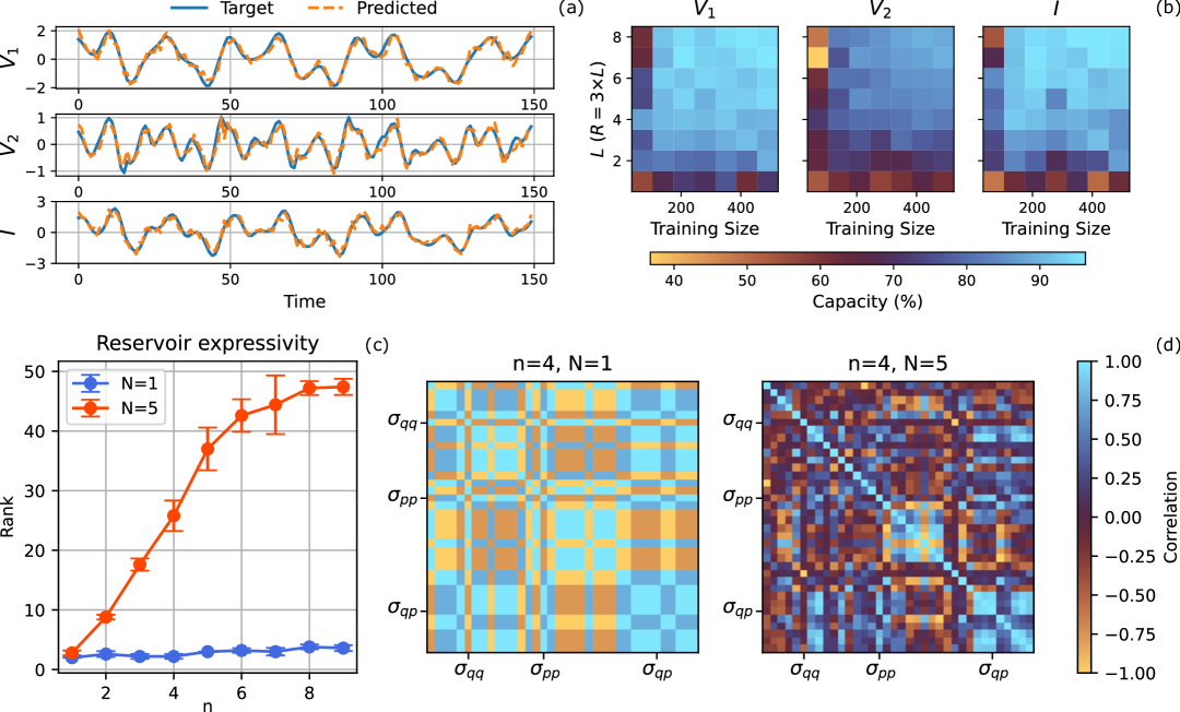
Figure 4: Double-scroll task (simulated). (a) Target (blue) and predicted (orange) trajectories using a realistic experimental noise model, with $15$ reservoirs and a training size of $350$. Prediction accuracies for $V_{1}$, $V_{2}$, and $I$ are $93.1\%$, $85.3\%$, and $90.7\%$, respectively. (b) Prediction capacity as a function of $L$ (number of reservoirs $=3L$) and training size, for $V_{1}$, $V_{2}$, and $I$. General phase encoding (simulated). (c) Rank of the observables matrix vs. number of measured modes $n$ (with $N$ input pump frexels), measuring reservoir expressivity (a.k.a. kernel quality). For $N=1$ (blue), increasing $n$ does not improve expressivity. Error bars reflect variations across random input sequences and parameters; fluctuations at $N=1$ mainly stem from numerical noise. (d) Correlation matrices between observables for $N=1$ and $N=5$ at $n=4$ ($2n$ quadrature operators, yielding $n(2n+1)=36$ observables). For $N=1$, only a few distinct correlations appear due to high redundancy; for $N=5$, correlations and thus observables behaviors are richer and more diverse.

Given the optimal agreement of the experiment with the numerical simulations, we use the Digital Twin to explore the performance of the protocol for a more complex task. Concretely, we perform a time-series forecasting task of the double-scroll electronic circuit [46]. It is a three-dimensional dynamical system (see the equations in the Appendix). As we deal with a $3$-dimensional input vector, we again have to use spatial multiplexing at least to encode each of the three signals as inputs. Thus, we need a minimum of $3$ spatially multiplexed reservoirs to process the whole input. We can add more spatially multiplexed reservoirs to enhance the expressivity. For the training phase, we consider the target function to be the input one timestep in the future: $\mathbf{\hat{y}}_{k}=\mathbf{s}_{k+1}$. Once the system has learned to forecast the signal, we feed the reservoir predictions as new inputs and check if the system is able to reproduce the test set. In plot (a) of Fig. 4, we present an example of target and predicted values, obtained with simulations with realistic noise values. Below, we present three plots (corresponding to $V_{1},V_{2},I$) where the capacity is calculated while varying the training size and the number of reservoirs $R$. We can see that, even with the experimental noise, we saturate the prediction capacity for relatively small values of $R$ and of training size.

II.3.2 General encoding: scaling the expressivity

Global phase encoding limitations can be assessed analytically showing that a boost in performance can be achieved diversifying the encoding in different modes. As shown analytically in Eq.(30) in the Appendix, when encoding on a global phase $\delta$, even if we increase the number of measured modes $n>1$, all the terms of the covariance matrix behave like either $\sin^{2}{\delta}$, $\cos^{2}{\delta}$ or $\cos{\delta}\sin{\delta}$. The expressivity of the reservoir is therefore limited for all $n$. This also happens when simulating the system with a detailed physical model that takes into account the characteristics of the parametric down conversion material and of the beams, as shown in the bottom part of Fig. 4, where we encode on a single pump band ($N=1$) and measure on $n$ output frequency bands (frexels). Indeed, to evaluate more quantitatively the expressivity of the system, we compute the rank of a matrix whose rows correspond to observables evaluated at different input states (see Sec. IV for a more precise expression). This rank, called kernel quality in the literature [44, 45, 47], would indicate the number of linearly independent observables, however since we scaled them beforehand, it also takes into account affine dependence. For linear regressions, an observable affine to another should not be useful. Since for a global phase, the observables behave like $\sin^{2}{\delta}=1-\cos^{2}{\delta}$, $\cos^{2}{\delta}$ or $\cos{\delta}\sin{\delta}$, analytically the rank should be equal to $2$ for all $n$, however numerical fluctuations of the code make it less stable. Nevertheless, we can still see that there are three behaviors only ($O_{A}\sim\cos^{2}{\delta}$, $O_{B}\sim-\cos^{2}{\delta}$ and $O_{C}\sim\cos{\delta}\sin{\delta}$) from the first subplot in (d) Fig. 4.

If instead we want to exploit the multimode nature of the system we see, in (c) and in the last subplot (d) of Fig. 4, for example, that we need to diversify as well the phase imprinted on the pump ($N>1$). This means exploiting fully the phase encoding from Eq.(4). With this general encoding ($N=9$), we successfully obtain capacities $>99.5\%$ for a parity check task for $\tau\in\{1,2,3\}$, as shown in Fig. 5 in the Appendix. We also exploit the multidimensionality of the input (it can be a vector of size up to $N$), to implement again the double scroll task, without multiplexing. The results are similar between the global phase encoding with multiplexing ($R=15$ reservoirs) and the general phase encoding with $N,n=9,9$. However, with the general encoding, we require no multiplexing and we use only one system, instead of $15$.

III Discussion

Starting from a multimode squeezed resource, we develop an optical quantum reservoir computing platform that leverages spectral shaping capabilities in femtosecond optics for both encoding and decoding information. Fading memory is enabled by linear feedback, even when limited to observables at one previous step. The continuous-variable (CV) setting is implemented via coherent homodyne detection, exploiting low-order quadrature moments as observables—an approach identified as offering polynomial advantage in QRC.

By tailoring the pump phase in the parametric process using an electro-optic modulator, we experimentally show online temporal processing with memory, performing both binary task in real time and continuous tasks via successful spatial multiplexing. We demonstrate the nonlinear processing capabilities of the quantum reservoir with a temporal XOR task, assess its memory capacity using continuous input signals, and evaluate its forecasting performance with the double-scroll benchmark. These results are fully reproduced by a Digital Twin, a detailed numerical model of the protocol that includes the properties of the nonlinear optical material, the optical processes, multimode and mode-selective detection schemes, and experimentally derived noise contributions. The Digital Twin enables exploration of the system’s capabilities with high fidelity.

The potential of the system’s multimode nature is further revealed by encoding information onto a richer phase profile of the pump. This allows consistent nonlinear processing, improved memory (as evidenced by a parity-check task), and accurate forecasting of a chaotic time series (double-scroll), confirming the advantages of utilizing the full multimode structure. Compared to a purely spatial multiplexing strategy, this approach shows superior scaling, revealing the potential of the system’s entangled multimode structure for enhanced performance.

IV Appendix

IV.1 Experiment

The experimental setup is presented in Fig. 1. We use a pulsed laser with a repetition rate of 100 MHz centered at 1560 nm, and a pulse duration of about 57 fs, which undergoes second harmonic generation in a periodically poled lithium niobate (ppLN) crystal to pump PDC in periodically poled potassium titanyl phosphate (ppKTP) waveguides of type 0. More details about the source can be found in [27]. In the setup of this work, an electro-optic modulator (iXblue NIR-800-LN-0.1) is used to set the phase of the pump beam for the global phase encoding. Phase lock is provided in order to encode information and measure the desired quadratures on phases (see Subsec. IV.6). The general multi-spectral phase encoding can be set via a pulse-shaping technique based on a spatial light modulator, as it is implemented in the homodyne setup to select the spectral basis of the measurement. The average value of squeezing measured in this setup is $-0.45$ dB, a reduced value compared to the one in [27] due to the dispersion introduced in the pump pulse by the fiber-based phase modulator. Such dispersion can be significantly reduced in future experiments by shortening the input and output fiber lengths. The antisqueezing is around $0.7$ dB because of losses.

IV.2 Simulations - Digital Twin

The simulation is based on the effective interaction Hamiltonian for the PDC process, which reads, as introduced in the main text:

$$\hat{H}\propto\int d\lambda_{S}\,d\lambda_{I}\,J(\lambda_{S},\lambda_{I})\,\hat{a}^{\dagger}(\lambda_{S})\hat{b}^{\dagger}(\lambda_{I})+\text{h.c.}$$ (9)

where $J(\lambda_{S},\lambda_{I})$ is the JSA, given by the product of the complex pump envelope $p(\lambda_{S},\lambda_{I})$ and the phase-matching function $\phi(\lambda_{S},\lambda_{I})$. The complex pump function $p(\lambda_{S},\lambda_{I})$ can actually be written as $p(\lambda_{p})$ because of energy conservation condition $\lambda_{p}=(1/\lambda_{S}+1/\lambda_{I})^{-1}$. It conveys the information in our protocols and is described in detail in Subsec. IV.3. For the pump, we employ a Gaussian amplitude with a phase profile segmented into $N$ sections, each assigned a distinct phase value. If $N=1$ we are applying a global phase $\delta$, such as we do experimentally with our electro-optical modulator. Instead, for $N>1$ we need a spatial light modulator, to encode a vector phase $\boldsymbol{\delta}=(\delta_{i})_{i=1}^{N}$ where each element is the phase of the corresponding frequency band of the pump. The phase-matching function instead captures the effect of dispersion and waveguide geometry and is computed as:

$$\phi(\lambda_{S},\lambda_{I})=\text{sinc}\left(\frac{L\,\Delta k(\lambda_{S},\lambda_{I})}{2}\right),$$ (10)

with $L$ the length of the nonlinear poled waveguide (ppKTP) and $\Delta k$ the phase mismatch given by:

$$\Delta k(\lambda_{S},\lambda_{I})=k_{P}\left(\lambda_{P}\right)-k_{S}(\lambda_{S})-k_{I}(\lambda_{I})-\frac{2\pi}{\Lambda},$$ (11)

where $\lambda_{P}^{-1}=\lambda_{S}^{-1}+\lambda_{I}^{-1}$ ensures energy conservation and $\Lambda$ is the poling period of the waveguide, calculated in order to minimize the mismatch around the central wavelengths of the experiment. Each wavenumber is given by $k_{X}(\lambda)=\frac{2\pi n_{X}(\lambda)}{\lambda}$, where $X\in\{P,S,I\}$, and $n_{X}(\lambda)$ is the effective refractive index, which depends on the material, polarization, and waveguide dimensions.

In our simulations, we use the Sellmeier equations for KTP, our biaxial crystal, to model the wavelength-dependent refractive indices along the principal axes $x$, $y$, and $z$. These equations take the empirical form:

$$n_{x}^{2}(\lambda) =X_{1}+\frac{X_{2}}{\lambda^{2}-X_{3}}+\frac{X_{4}}{\lambda^{2}-X_{5}},$$ (12)

$$n_{y}^{2}(\lambda) =Y_{1}+\frac{Y_{2}}{\lambda^{2}-Y_{3}}+\frac{Y_{4}}{\lambda^{2}-Y_{5}},$$ (13)

$$n_{z}^{2}(\lambda) =Z_{1}+\frac{Z_{2}}{\lambda^{2}-Z_{3}}+\frac{Z_{4}}{\lambda^{2}-Z_{5}},$$ (14)

where the coefficients $X_{i}$, $Y_{i}$, and $Z_{i}$ are experimentally determined constants taken from Ref. [48]. Corrections are also included to account for the effect of waveguide confinement, which modifies the effective refractive index depending on the mode dimensions. The polarization of the fields (horizontal or vertical) is associated with the appropriate axis depending on the phase-matching type (Type-0, I, or II), which determines whether the pump, signal, and idler share the same or different polarization states. In our experiment, we use Type-0 waveguides.

To simulate the quantum output, we perform a singular value decomposition (SVD) of the JSA:

$$J(\lambda_{S},\lambda_{I})=\sum_{k}r_{k}\,h_{k}(\lambda_{S})\,g_{k}(\lambda_{I}).$$ (15)

This yields two orthonormal sets of spectral modes $\{h_{k}\}$ and $\{g_{k}\}$, associated with the signal and idler fields, respectively, and a corresponding set of Schmidt coefficients $\{r_{k}\}$. These modes define a new broadband mode basis through the operators:

$$\hat{A}_{k}^{\dagger}=\int d\lambda_{S}\,h_{k}(\lambda_{S})\,\hat{a}^{\dagger}(\lambda_{S}),\quad\hat{B}_{k}^{\dagger}=\int d\lambda_{I}\,g_{k}(\lambda_{I})\,\hat{b}^{\dagger}(\lambda_{I}).$$ (16)

In the degenerate case relevant to our experiment, where signal and idler are indistinguishable, we have $h_{k}=g_{k}$ and $\hat{A}_{k}^{\dagger}=\hat{B}_{k}^{\dagger}$, and the Hamiltonian simplifies to:

$$\hat{H}\propto\sum_{k}r_{k}\,\hat{A}_{k}^{\dagger 2}+\text{h.c.}$$ (17)

confirming the multimode squeezed output state.

To model the effect of measurement in a different basis (see Subsec. IV.3 for more details), we construct a mode transformation matrix $U$ that maps the natural Schmidt basis of the photon pair source to user-defined measurement bins. Formally the new mode basis basis $\xi_{j}(\lambda_{S})$ with creation operators $\hat{C}_{j}^{\dagger}$ is given by $\{\hat{C}_{j}^{\dagger}=\sum_{j}U_{jk}\hat{A}_{k}^{\dagger};\;\xi_{j}(\lambda_{S})=\sum_{j}U_{jk}h_{k}(\lambda_{S})\}$. Each element of $U$ is computed by integrating a Schmidt mode over the spectral range of a given frequency band (frexel) using the midpoint rule. The columns of $U$ are then normalized. To simulate quadrature measurements, we construct the associated symplectic matrix $\boldsymbol{S_{U}}$, which operates on the covariance matrix in the grouped ordering $[q_{1},\ldots,q_{n},p_{1},\ldots,p_{n}]$. The matrix $\boldsymbol{S_{U}}$ is built from the real and imaginary parts of $U$ as:

$$\boldsymbol{S_{U}}=\begin{pmatrix}\mathrm{Re}(U)&-\mathrm{Im}(U)\\ \mathrm{Im}(U)&\mathrm{Re}(U)\end{pmatrix}.$$ (18)

The covariance matrix in the measurement basis is then obtained via a congruence transformation:

$$\sigma_{\text{frexel}}=\boldsymbol{S_{U}}^{\mathrm{T}}\,\text{diag}\{e^{2r_{1}},e^{2r_{2}},...,e^{2r_{n}},e^{-2r_{1}},e^{-2r_{2}},...,e^{-2r_{n}}\}\,\boldsymbol{S_{U}}=\boldsymbol{\sigma}^{\prime}(U,p),$$ (19)

Our observables correspond to a subset of the elements in $\sigma_{\text{frexel}}$ since while they depend nonlinearly on the pump phase profile, they can be affine functions of each other, leading to redundancy.

For the case $N=1$, where the information is encoded in the global phase of the pump, analytical expressions for the observables are available (see Subsec. IV.5). In this regime, using the full simulation pipeline would be excessive, so we instead implemented a simplified model based directly on the analytical formulas, with the addition of Gaussian noise, with equivalent results. The noise parameters were estimated by fitting to the experimental data using the least-squares method. We also adjusted the squeezing parameters ($r_{k}$) and the phase dependence to match the experimental values and results. These simulations were also useful to establish the range of parameters $\alpha,\beta,M$ used in the experiment to encode information on the phase.

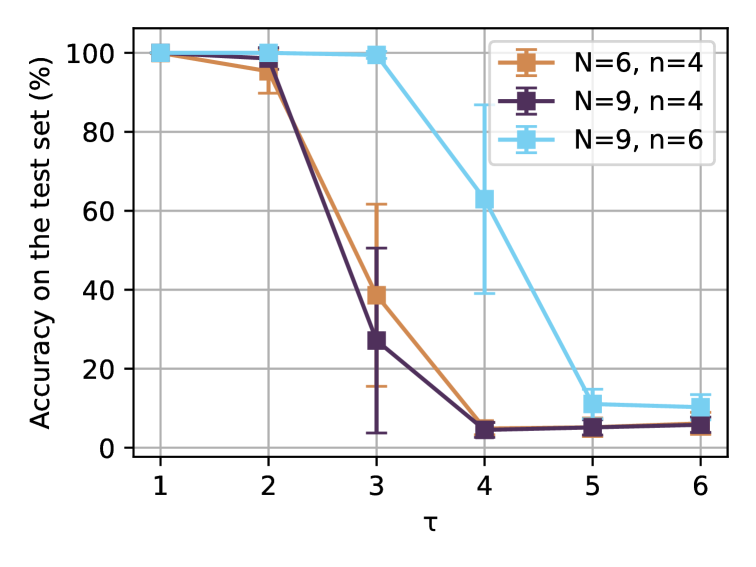
Figure 5: Parity check task (simulated results) with the general encoding. Parity check accuracy for different delays $\tau$ and for different combinations of $N$ (the number of phase segments we imprint on the pump) and $n$ (the number of measured output modes). The error bars are obtained by repeating the simulation with random parameters $10$ times.

IV.3 $N$ input modes and $n$ output modes

Let us consider a Gaussian pump profile $f(\lambda_{P})$ of width $\sigma$ and central wavelength $\lambda_{P}^{c}$. Let $N$ be the dimension of our input space, that is to say the number of pump frequency modes.

The frequency modes $f_{i}(\lambda_{P})$ ($i=1,\dots,N$) considered in the simulations — and implementable using a spatial light modulator — are defined as:

$$f_{i}(\lambda_{P})=\begin{cases}f(\lambda_{P})&\text{if }\lambda_{P}\in\left[\lambda_{P}^{c}-3\sigma+6\sigma\frac{i}{N},\;\lambda_{P}^{c}-3\sigma+6\sigma\frac{i+1}{N}\right]\\ 0&\text{otherwise}\end{cases}$$ (20)

In other words, the total $6\sigma$-wide Gaussian pump is divided into $N$ contiguous, non-overlapping frequency segments (frexels).

Concerning the $n$ measurement modes, for the simulations with the general encoding ($N>1$) we use as measurement modes frequency bands (frexels again). If the Schmidt basis is centered around $\lambda^{c}=2\lambda_{P}^{c}$, we consider an interval $[-S,S]$ centered on $\lambda^{c}$ such that it includes the main features of the first $n$ Schmidt modes.

The frexels are defined as:

$$\xi_{j}(\lambda)=\begin{cases}1&\text{if }\lambda\in\left[\lambda^{c}-S+\frac{2Sj}{n},\;\lambda^{c}-S+\frac{2S(j+1)}{n}\right]\\ 0&\text{otherwise}\end{cases}$$ (21)

That is, each measurement mode corresponds to a rectangular frequency band and together the $n$ modes form a uniform partition of the interval $[\lambda^{c}-S,\;\lambda^{c}+S]$, covering the spectral region where the Schmidt modes are significantly supported. This can be easily implemented again with the spatial light modulator on the local oscillator. Here, the amplitude is set to $1$ because in the simulations everything is normalized after the calculation of the JSA.

The effect of this choice of measurement modes is calculated in the matrix $U$, where the $h_{i}(\lambda)$ are the Schmidt modes:

$$U_{ij}=\int h_{i}(\lambda)\,\xi_{j}(\lambda)\,d\lambda$$ (22)

When each measurement mode $\xi_{j}(\lambda)$ is a frexel this simplifies to:

$$U_{ij}=\int_{\lambda^{c}-S+\frac{2Sj}{n}}^{\lambda^{c}-S+\frac{2S(j+1)}{n}}h_{i}(\lambda)\,d\lambda$$ (23)

That is, $U_{ij}$ quantifies the overlap between the $i$-th Schmidt mode and the $j$-th measurement frequency band. The matrix $U$ therefore describes how the original modal structure is projected onto the coarse-grained measurement basis and enables the computation of the corresponding covariance matrix in simulations. The rows of $U$ are normalized to preserve unitarity as closely as possible. However, since the Schmidt modes form a complete (infinite-dimensional) basis and the measurement modes form a finite set—even if they are orthogonal and span the same subspace—the matrix $U$ does not represent an exact change of basis. Rather, it provides a truncated, approximate mapping suitable for finite-dimensional analysis.

Figure 5 illustrates how access to $N$ input modes and $n$ output modes influences performance, using the parity check task as an example. The general encoding across multiple input modes yields a performance boost as the number of measured output modes increases.

IV.4 Regressions and metrics

To train a reservoir computer we use regressions to combine the observables in a way that mimics a target function. Indeed, we compare a predicted output $y$ with a target output $\hat{y}$, of length $M$.

For binary tasks, where each prediction is either 0 or 1, we use a linear regression initially:

$$y_{k}=\mathbf{w}^{T}\mathbf{O}^{(k)}+b$$ (24)

However, before evaluating the performance, we apply a threshold at 0.5 to obtain binary predictions:

$${y^{\prime}}_{k}=\begin{cases}1&\text{if }y_{k}>0.5,\\ 0&\text{otherwise}.\end{cases}$$ (25)

We evaluate the performance of the system with the accuracy, defined as the fraction of correct predictions:

$$\text{Accuracy}=\frac{1}{M}\sum_{i=1}^{M}\delta\left(y^{\prime}_{i},\hat{y}_{i}\right)$$ (26)

where $\delta(a,b)$ is the Kronecker delta function, equal to 1 if $a=b$ and 0 otherwise.

For continuous tasks, we use a linear regression directly:

$$y_{k}=\mathbf{w}^{T}\mathbf{O}^{(k)}+b$$ (27)

To evaluate the performance, we use here the capacity, which is defined as the squared Pearson correlation coefficient between the predicted output $y$ and the target output $\hat{y}$ (as in [49]):

$$\text{Capacity}=\left(\text{corr}(y,\hat{y})\right)^{2}=\left(\frac{\text{Cov}(y,\hat{y})}{\sigma_{y}\sigma_{\hat{y}}}\right)^{2}$$ (28)

Concerning the expressivity, let $\sigma^{\prime}_{k}$ be the covariance matrix obtained at timestep $k$ from the encoded input $s_{k}$ and feedback in the measurement basis. We construct a matrix $\mathcal{O}\in\mathbb{R}^{d\times d}$, where each row contains the elements of the covariance (there are at most $d=n(2n+1)$ unique elements) for $d$ steps after some washout inputs. We scale the observables and we define:

$$\mathrm{rank}(\mathcal{O})=\#\{\lambda_{i}>\varepsilon\ |\ \lambda_{i}\text{ is a singular value of }\mathcal{O}\}=\text{kernel quality}$$

where the rank is computed with a numerical tolerance $\varepsilon=10^{-4}$. This rank, often called kernel quality, indicates how well the reservoir represents different input streams and it can be used as a measure for the complexity and diversity of nonlinear operations performed, that is to say the expressivity of the reservoir [44, 45, 47]. The rank defines the number of observables that are not linearly dependent (after scaling).

IV.5 Analytical expressions of the global phase encoding

Let us see what happens when measuring more than one mode, that is to say, $n>1$, for the global phase encoding. The set of the $n$ measurement modes is related to the Schmidt modes by $U$. To simplify the notations, we restrict ourselves to the case where $U$ is real.

The covariance matrix of the system becomes:

$$\sigma(\delta,U)=\begin{bmatrix}\sigma_{0,0}(\delta,U)&\sigma_{0,1}(\delta,U)&\dots\\ \vdots&\ddots&\\ \sigma_{n-1,0}(\delta,U)&&\sigma_{n-1,n-1}(\delta,U)\end{bmatrix}$$ (29)

Where $\sigma_{l,j}(\delta,U)$ is a 2x2 matrix:

$$\sigma_{l,j}(\delta,U)=\sum_{a=1}^{n}U_{j,a}U_{l,a}\begin{bmatrix}e^{2r_{a}}+(e^{-2r_{a}}-e^{2r_{a}})\sin^{2}{\delta}&(e^{2r_{a}}-e^{-2r_{a}})\cos{\delta}\sin{\delta}\\ (e^{2r_{a}}-e^{-2r_{a}})\cos{\delta}\sin{\delta}&e^{2r_{a}}+(e^{-2r_{a}}-e^{2r_{a}})\cos^{2}{\delta}\end{bmatrix}$$ (30)

We see that all the terms of the covariance matrix are affine functions of either $\sin^{2}{\delta}$, $\cos^{2}{\delta}$, or $\cos{\delta}\sin{\delta}$, reflecting the phase dependence introduced by the rotation in phase space.

Let us restrict ourselves to the case $n=1$ for simplicity, the rotated quadrature variance along the direction $(\hat{q}+\hat{p})/\sqrt{2}$ is given by

$$\langle\Delta(\frac{\hat{q}+\hat{p}}{\sqrt{2}})^{2}\rangle=\frac{1}{2}\left(\langle\Delta\hat{q}^{2}\rangle+\langle\Delta\hat{p}^{2}\rangle+2\langle\Delta\hat{q}\Delta\hat{p}\rangle\right)=\frac{1}{2}(2e^{-2r}+2(e^{2r}-e^{-2r})\cos\delta\sin\delta)=\langle\Delta\hat{q}\Delta\hat{p}\rangle+cst$$ (31)

IV.6 Phase locking and acquisition process

Since our protocol relies on encoding information in the squeezing phase and on measuring precise elements of the covariance matrix, it is essential to stabilize both the pump phase and the local oscillator (LO) phase. The phase of the local oscillator $\theta_{LO}$ with respect to a fixed reference, that we conveniently call $\phi_{S}$, determines the quadrature measured via homodyne detection: $\hat{x}({\theta_{\text{LO}}})=\cos(\theta_{LO})\hat{q}+\sin(\theta_{\text{LO}})\hat{p}$.

To achieve phase stabilization, a third beam, termed the seed, is introduced at the same wavelength as the LO. Since irrelevant during the actual squeezing measurements (which involve vacuum modes), the seed is periodically blocked during designated measurement times. In the alternating locking times, it is instead unblocked and used to actively monitor and stabilize the pump and LO phases. The detection is left inactive during the locking times, thanks to a gate function of the instruments (gating the measurement times).

The seed follows the same optical path as the pump and interacts with it in the nonlinear waveguide via amplification and deamplification. These oscillations in the seed (and pump) amplitude are monitored and are proportional to:

$$\cos(\phi_{P}-2\phi_{S})$$ (32)

where $\phi_{P}$ and $\phi_{S}$ are the pump and seed phases, respectively. This signal is used in a feedback loop via a PID controller to lock the phase difference. During the locking times, the phase modulator used to encode the information is disabled via an analog switch, ensuring that the encoded phase difference $\delta$ remains unchanged (not compensated by the PID).

The seed also interferes on its path with the LO, generating a signal known as visibility, which is sensitive to $\phi_{\text{LO}}$ because it is proportional to:

$$\cos(\phi_{\text{LO}}-\phi_{S})=\cos{\theta_{LO}}$$ (33)

While this signal can be locked with a PID loop to a specific setpoint, corresponding to a given quadrature measurement, we opted for a more flexible approach. Instead of alternating multiple lock points, we scan the LO phase and post-select the squeezing measurements based on the value of the visibility signal, as illustrated in Fig. 6. The visibility is seen on an oscilloscope on a leak after the balanced beam splitter of the homodyne detection, where seed and LO interact. The variance of the homodyne signal is measured with a spectrum analyzer, synchronized with the oscilloscope and the locking/measurement phases. Indeed, the spectrum analyzer calculates the variance of the input signal when used in zero-span, which gives us our observables directly.

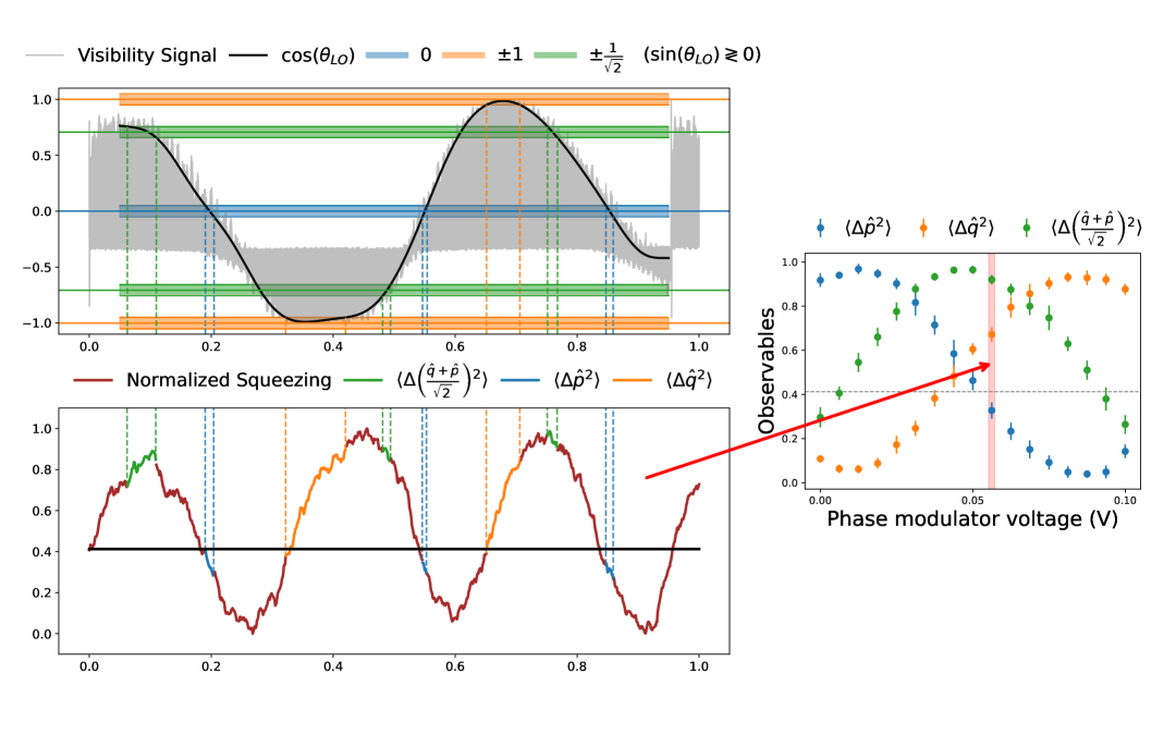
Figure 6: Experimental acquisition process and phase dependence. On the left oscilloscope (top) and spectrum analyzer (bottom) normalized acquisitions for a single global pump phase. The visibility, acquired with the oscilloscope, is normalized between -1 and 1 as a cosine. The variance of the homodyne signal is normalized between 0 and 1 (to have already scaled observables). The values of the visibility cosine dictate what quadrature we are measuring ($\hat{x}_{\theta_{\text{LO}}}=\cos(\theta_{LO})\hat{q}+\sin(\theta_{\text{LO}})\hat{p}$), we take the corresponding times on the spectrum analyzer signal to reconstruct an average value of the covariance elements for the selected global phase (in dB). These averages become our observables. On the right the results of these acquisitions when scanning the global phase of the pump with the modulator and by repeating $10$ times the acquisition on the left.

IV.7 Parameters $\alpha,\beta$ and feedback mask

From the lower subplot of Fig. 1, we estimate that achieving the full modulation range of observables (from 0 to 1 or vice versa, so a $\delta$ span of $\pi/2$) requires a voltage span of approximately $V_{\pi/2}=0.075~\mathrm{V}$. This value sets the scale for the input and feedback parameters used across tasks. The global phase of the pump, $\delta$, depends indeed on the voltage $V$ applied to the EOM as $\delta(V)=\frac{\pi}{2}\cdot\frac{V}{V_{\pi/2}}+\text{offset}$.

XOR Task

For the XOR task, the following parameters were used:

• Input ($s_{k}\in\{0,1\}$) coefficient: $\alpha=V_{\pi/2}$,

• Offset: $\beta=-0.01$ (a small offset with negligible effect on performance),

• Feedback coefficient (scalar): $M=0.035\approx 0.46\,V_{\pi/2}$.

Memory Task

No offset was applied for the memory task, i.e., $\beta_{r}=0$ for all $r$. The feedback strengths $\alpha_{r}$, grouped in a vector $\vec{\alpha}\in\mathbb{R}^{R}$, and the feedback mask matrices $M_{r,r^{\prime}}\in\mathbb{R}^{R\times R}$, were drawn randomly and scaled (multiplied) by $V_{\pi/2}$. The specific values before scaling are:

• For $R=5$:

  $$\vec{\alpha} =\begin{bmatrix}-0.17&-0.37&-0.31&-0.14&-0.3\end{bmatrix},\quad M=\begin{bmatrix}-0.39&0.16&-0.34&0.17&0.32\\ 0.45&-0.21&0.13&0.43&0.32\\ -0.11&0.50&0.29&0.45&0.06\\ 0.32&0.23&-0.06&-0.47&0.47\\ -0.26&-0.01&-0.17&-0.12&0.33\end{bmatrix}$$

• For $R=3$:

  $$\vec{\alpha} =\begin{bmatrix}0.25&0.34&-0.32\end{bmatrix},\quad M=\begin{bmatrix}0.33&-0.02&-0.34\\ -0.50&-0.28&0.29\\ -0.40&-0.48&-0.35\end{bmatrix}$$

• For $R=1$:

  $$\vec{\alpha} =\begin{bmatrix}-0.25\end{bmatrix},\quad M=\begin{bmatrix}0.87\end{bmatrix}$$

Double Scroll Task

For the double scroll task, no offset was applied. The feedback vector $\vec{\alpha}$ was initialized randomly in the interval $[-w,w]$ with $w=1.25$. The feedback mask $M$ was drawn from a uniform distribution over $[-1,1]$, normalized by its largest singular value, and scaled by a factor of 0.7. All values were then multiplied by $V_{\pi/2}$.

General Encoding

The general encoding used in all tasks included:

• Delay time: $\delta_{\text{amp}}=10^{-16}~\mathrm{s}$,

• Random vectors $\vec{\alpha}$ and $\vec{\beta}$ of length $N$, with entries uniformly sampled from $[-1,1]$ and multiplied by $\delta_{\text{amp}}$,

• Feedback mask matrix $M$ with entries in $[0,2]$, normalized by its largest singular value, scaled by a factor $m=0.4$ and multiplied by $\delta_{\text{amp}}$.

IV.8 Double scroll ODEs

The system of ODEs to generate the data for the double-scroll task reads

$$\dot{V}_{1} =V_{1}/R_{1}-\Delta V/R_{2}-2I_{r}\sinh(\beta\Delta V),$$ (34)

$$\dot{V}_{2} =\Delta V/R_{2}+2I_{r}\sinh(\beta\Delta V)-I,$$

$$\dot{I} =V_{2}-R_{4}I\ ,$$

where $\Delta V=V_{1}-V_{2}$, $(R_{1},R_{2},R_{4})=(1.2,3.44,0.193)$, $\beta=11.6$ and $I_{r}=2.25\times 10^{-5}$. We consider the input vector at each time step to be $\mathbf{s}_{k}=\left[V_{1}(k\Delta t),V_{2}(k\Delta t),I(k\Delta t)\right]^{\top}$. In our case, the sampling interval is $\Delta t=1$.

References

- [1] Mantas Lukoševičius and Herbert Jaeger. Reservoir computing approaches to recurrent neural network training. Computer science review, 3(3):127–149, 2009.
- [2] Kohei Nakajima and Ingo Fischer. Reservoir Computing: Theory, Physical Implementations, and Applications. Springer Nature, 2021.
- [3] John B Butcher, David Verstraeten, Benjamin Schrauwen, Charles R Day, and Peter W Haycock. Reservoir computing and extreme learning machines for non-linear time-series data analysis. Neural networks, 38:76–89, 2013.
- [4] Silvia Ortín, Miguel C. Soriano, Luis Pesquera, Daniel Brunner, Daniel San-Martín, Ingo Fischer, Claudio R Mirasso, and José M Gutiérrez. A unified framework for reservoir computing and extreme learning machines based on a single time-delayed neuron. Scientific reports, 5(1):14945, 2015.
- [5] Pere Mujal, Rodrigo Martínez-Peña, Johannes Nokkala, Jorge García-Beni, Gian Luca Giorgi, Miguel C. Soriano, and Roberta Zambrini. Opportunities in quantum reservoir computing and extreme learning machines. Advanced Quantum Technologies, 4(8):2100027, 2021.
- [6] Sanjib Ghosh, Kohei Nakajima, Tanjung Krisnanda, Keisuke Fujii, and Timothy CH Liew. Quantum neuromorphic computing with reservoir computing networks. Advanced Quantum Technologies, 4(9):2100053, 2021.
- [7] Adrià Labay-Mora, Jorge García-Beni, Gian Luca Giorgi, Miguel C. Soriano, and Roberta Zambrini. Neural networks with quantum states of light. Philosophical Transactions A, 382(2287):20230346, 2024.
- [8] Akitada Sakurai, Aoi Hayashi, William John Munro, and Kae Nemoto. Quantum optical reservoir computing powered by boson sampling. Optica Quantum, 3(3):238–245, 2025.
- [9] Keisuke Fujii and Kohei Nakajima. Harnessing disordered-ensemble quantum dynamics for machine learning. Phys. Rev. Appl., 8:024030, Aug 2017.
- [10] Alen Senanian, Sridhar Prabhu, Vladimir Kremenetski, Saswata Roy, Yingkang Cao, Jeremy Kline, Tatsuhiro Onodera, Logan G. Wright, Xiaodi Wu, Valla Fatemi, and Peter L. McMahon. Microwave signal processing using an analog quantum reservoir computer. Nature Communications, 15(1):7490, Aug 2024.
- [11] Johannes Nokkala, Gian Luca Giorgi, and Roberta Zambrini. Retrieving past quantum features with deep hybrid classical-quantum reservoir computing. Machine Learning: Science and Technology, 3(5):035022, 2024.
- [12] Luca Innocenti, Salvatore Lorenzo, Ivan Palmisano, Alessandro Ferraro, Mauro Paternostro, and G Massimo Palma. Potential and limitations of quantum extreme learning machines. Communications Physics, 6(1):118, 2023.
- [13] Pere Mujal, Rodrigo Martínez-Peña, Gian Luca Giorgi, Miguel C. Soriano, and Roberta Zambrini. Time-series quantum reservoir computing with weak and projective measurements. npj Quantum Information, 9(1):16, 2023.
- [14] Antonio Sannia, Gian Luca Giorgi, and Roberta Zambrini. Exponential concentration and symmetries in quantum reservoir computing. arXiv preprint arXiv:2505.10062, 2025.
- [15] Bhavin J. Shastri, Alexander N. Tait, T. Ferreira de Lima, Wolfram H. P. Pernice, Harish Bhaskaran, C. D. Wright, and Paul R. Prucnal. Photonics for artificial intelligence and neuromorphic computing. Nature Photonics, 15(2):102–114, 2021.
- [16] Jorge García-Beni, Gian Luca Giorgi, Miguel C. Soriano, and Roberta Zambrini. Scalable photonic platform for real-time quantum reservoir computing. Phys. Rev. Appl., 20:014051, Jul 2023.
- [17] Alessia Suprano, Danilo Zia, Luca Innocenti, Salvatore Lorenzo, Valeria Cimini, Taira Giordani, Ivan Palmisano, Emanuele Polino, Nicolò Spagnolo, Fabio Sciarrino, G. Massimo Palma, Alessandro Ferraro, and Mauro Paternostro. Experimental property reconstruction in a photonic quantum extreme learning machine. Phys. Rev. Lett., 132:160802, Apr 2024.
- [18] Danilo Zia, Luca Innocenti, Giorgio Minati, Salvatore Lorenzo, Alessia Suprano, Rosario Di Bartolo, Nicolò Spagnolo, Taira Giordani, Valeria Cimini, G. Massimo Palma, Alessandro Ferraro, Fabio Sciarrino, and Mauro Paternostro. Quantum extreme learning machines for photonic entanglement witnessing, February 2025.
- [19] Valeria Cimini, Mandar M. Sohoni, Federico Presutti, Benjamin K. Malia, Shi-Yuan Ma, Ryotatsu Yanagimoto, Tianyu Wang, Tatsuhiro Onodera, Logan G. Wright, and Peter L. McMahon. Large-scale quantum reservoir computing using a gaussian boson sampler, May 2025.
- [20] Sam Nerenberg, Oliver D Neill, Giulia Marcucci, and Daniele Faccio. Photon number-resolving quantum reservoir computing. Optica Quantum, 3(2):201–210, 2025.
- [21] Longhan Wang, Peijie Sun, Ling-Jun Kong, Yifan Sun, and Xiangdong Zhang. Quantum next-generation reservoir computing and its quantum optical implementation. Phys. Rev. A, 111:022609, Feb 2025.
- [22] Kaito Kobayashi, Keisuke Fujii, and Naoki Yamamoto. Feedback-driven quantum reservoir computing for time-series analysis. PRX Quantum, 5:040325, Nov 2024.
- [23] Tomoya Monomi, Wataru Setoyama, and Yoshihiko Hasegawa. Feedback-enhanced quantum reservoir computing with weak measurements. arXiv preprint arXiv:2503.17939, 2025.
- [24] Fangjun Hu, Saeed A. Khan, Nicholas T. Bronn, Gerasimos Angelatos, Graham E. Rowlands, Guilhem J. Ribeill, and Hakan E. Türeci. Overcoming the coherence time barrier in quantum machine learning on temporal data. Nature Communications, 15(1), August 2024.
- [25] Mirela Selimović, Iris Agresti, Michał Siemaszko, Joshua Morris, Borivoje Dakić, Riccardo Albiero, Andrea Crespi, Francesco Ceccarelli, Roberto Osellame, Magdalena Stobińska, and Philip Walther. Experimental neuromorphic computing based on quantum memristor. 2025.
- [26] Tiphaine Kouadou, Francesca Sansavini, Matthieu Ansquer, Johan Henaff, Nicolas Treps, and Valentina Parigi. Spectrally shaped and pulse-by-pulse multiplexed multimode squeezed states of light. APL Photonics, 8(8), 2023.
- [27] Victor Roman-Rodriguez, David Fainsin, Guilherme L Zanin, Nicolas Treps, Eleni Diamanti, and Valentina Parigi. Multimode squeezed state for reconfigurable quantum networks at telecommunication wavelengths. Physical Review Research, 6(4):043113, 2024.
- [28] P. Renault, J. Nokkala, G. Roeland, N.Y. Joly, R. Zambrini, S. Maniscalco, J. Piilo, N. Treps, and V. Parigi. Experimental optical simulator of reconfigurable and complex quantum environment. PRX Quantum, 4:040310, Oct 2023.
- [29] Johannes Nokkala, Rodrigo Martínez-Peña, Gian Luca Giorgi, Valentina Parigi, Miguel C. Soriano, and Roberta Zambrini. Gaussian states of continuous-variable quantum systems provide universal and versatile reservoir computing. Communications Physics, 4(1):53, Mar 2021.
- [30] Jorge García-Beni, Gian Luca Giorgi, Miguel C. Soriano, and Roberta Zambrini. Squeezing as a resource for time series processing in quantum reservoir computing. Opt. Express, 32(4):6733–6747, Feb 2024.
- [31] Jorge García-Beni, Iris Paparelle, Valentina Parigi, Gian Luca Giorgi, Miguel C. Soriano, and Roberta Zambrini. Quantum machine learning via continuous-variable cluster states and teleportation. EPJ Quantum Technology, 12(1):63, Jun 2025.
- [32] Johan Henaff, Matthieu Ansquer, Miguel C. Soriano, Roberta Zambrini, Nicolas Treps, and Valentina Parigi. Optical phase encoding in a pulsed approach to reservoir computing. Opt. Lett., 49(8):2097–2100, Apr 2024.
- [33] Young-Sik Ra, Adrien Dufour, Mattia Walschaers, Clément Jacquard, Thibault Michel, Claude Fabre, and Nicolas Treps. Non-Gaussian quantum states of a multimode light field. Nature Physics, 16(2):144–147, February 2020.
- [34] Maria Schuld and Nathan Killoran. Is quantum advantage the right goal for quantum machine learning? PRX Quantum, 3:030101, Jul 2022.
- [35] J. Eli Bourassa, Rafael N. Alexander, Michael Vasmer, Ashlesha Patil, Ilan Tzitrin, Takaya Matsuura, Daiqin Su, Ben Q. Baragiola, Saikat Guha, Guillaume Dauphinais, Krishna K. Sabapathy, Nicolas C. Menicucci, and Ish Dhand. Blueprint for a Scalable Photonic Fault-Tolerant Quantum Computer. Quantum, 5:392, February 2021.
- [36] Miller Eaton, Carlos González-Arciniegas, Rafael N. Alexander, Nicolas C. Menicucci, and Olivier Pfister. Measurement-based generation and preservation of cat and grid states within a continuous-variable cluster state. Quantum, 6:769, July 2022.
- [37] Matthew S. Winnel, Joshua J. Guanzon, Deepesh Singh, and Timothy C. Ralph. Deterministic preparation of optical squeezed cat and gottesman-kitaev-preskill states. Phys. Rev. Lett., 132:230602, Jun 2024.
- [38] Amanuel Anteneh, Léandre Brunel, and Olivier Pfister. Machine learning for efficient generation of universal photonic quantum computing resources. Optica Quantum, 2(4):296–302, Aug 2024.
- [39] M. V. Larsen, J. E. Bourassa, S. Kocsis, J. F. Tasker, R. S. Chadwick, C. González-Arciniegas, J. Hastrup, C. E. Lopetegui-González, F. M. Miatto, A. Motamedi, R. Noro, G. Roeland, R. Baby, H. Chen, P. Contu, I. Di Luch, C. Drago, M. Giesbrecht, T. Grainge, I. Krasnokutska, M. Menotti, B. Morrison, C. Puviraj, K. Rezaei Shad, B. Hussain, J. McMahon, J. E. Ortmann, M. J. Collins, C. Ma, D. S. Phillips, M. Seymour, Q. Y. Tang, B. Yang, Z. Vernon, R. N. Alexander, and D. H. Mahler. Integrated photonic source of Gottesman–Kitaev–Preskill qubits. Nature, June 2025.
- [40] Benjamin Brecht, Dileep V Reddy, Christine Silberhorn, and Michael G Raymer. Photon temporal modes: a complete framework for quantum information science. Physical Review X, 5(4):041017, 2015.
- [41] V Roman-Rodriguez, B Brecht, C Silberhorn, N Treps, E Diamanti, V Parigi, et al. Continuous variable multimode quantum states via symmetric group velocity matching. New Journal of Physics, 23(4):043012, 2021.
- [42] Francesco Arzani, Claude Fabre, and Nicolas Treps. Versatile engineering of multimode squeezed states by optimizing the pump spectral profile in spontaneous parametric down-conversion. Phys. Rev. A, 97:033808, Mar 2018.
- [43] Y. Cai, J. Roslund, G. Ferrini, F. Arzani, X. Xu, C. Fabre, and N. Treps. Multimode entanglement in reconfigurable graph states using optical frequency combs. Nature Communications, 8(1):15645, Jun 2017.
- [44] Lennert Appeltant et al. Reservoir computing based on delay-dynamical systems. These de Doctorat, Vrije Universiteit Brussel/Universitat de les Illes Balears, 2012.
- [45] Parami Wijesinghe, Gopalakrishnan Srinivasan, Priyadarshini Panda, and Kaushik Roy. Analysis of liquid ensembles for enhancing the performance and accuracy of liquid state machines. Frontiers in neuroscience, 13:504, 2019.
- [46] Daniel J. Gauthier, Erik Bollt, Aaron Griffith, and Wendson A. S. Barbosa. Next generation reservoir computing. Nature Communications, 12(1):5564, Sep 2021.
- [47] Chester Wringe, Martin Trefzer, and Susan Stepney. Reservoir computing benchmarks: a tutorial review and critique. International Journal of Parallel, Emergent and Distributed Systems, pages 1–39, 2025.
- [48] Kiyoshi Kato and Eiko Takaoka. Sellmeier and thermo-optic dispersion formulas for ktp. Applied optics, 41(24):5040–5044, 2002.
- [49] Rodrigo Martínez-Peña, Gian Luca Giorgi, Johannes Nokkala, Miguel C. Soriano, and Roberta Zambrini. Dynamical phase transitions in quantum reservoir computing. Physical Review Letters, 127(10):100502, 2021.