ALINE: Joint Amortization for Bayesian Inference and Active Data Acquisition

Abstract

Many critical applications, from autonomous scientific discovery to personalized medicine, demand systems that can both strategically acquire the most informative data and instantaneously perform inference based upon it. While amortized methods for Bayesian inference and experimental design offer part of the solution, neither approach is optimal in the most general and challenging task, where new data needs to be collected for instant inference. To tackle this issue, we introduce the Amortized Active Learning and Inference Engine (Aline), a unified framework for amortized Bayesian inference and active data acquisition. Aline leverages a transformer architecture trained via reinforcement learning with a reward based on self-estimated information gain provided by its own integrated inference component. This allows it to strategically query informative data points while simultaneously refining its predictions. Moreover, Aline can selectively direct its querying strategy towards specific subsets of model parameters or designated predictive tasks, optimizing for posterior estimation, data prediction, or a mixture thereof. Empirical results on regression-based active learning, classical Bayesian experimental design benchmarks, and a psychometric model with selectively targeted parameters demonstrate that Aline delivers both instant and accurate inference along with efficient selection of informative points.

1 Introduction

Bayesian inference (Gelman et al.,, 2013) and Bayesian experimental design (Rainforth et al.,, 2024) offer principled mathematical means for reasoning under uncertainty and for strategically gathering data, respectively. While both are foundational, they both introduce notorious computational challenges. For example, in scenarios with continuous data streams, repeatedly applying gold-standard inference methods such as Markov Chain Monte Carlo (MCMC) (Carpenter et al.,, 2017) to update posterior distributions can be computationally demanding, leading to various approximate sequential inference techniques (Broderick et al.,, 2013; Doucet et al.,, 2001), yet challenges in achieving both speed and accuracy persist. Similarly, in Bayesian experimental design (BED) or Bayesian active learning (BAL), the iterative estimation and optimization of design objectives can become costly, especially in sequential learning tasks requiring rapid design decisions (Filstroff et al.,, 2024; Giovagnoli,, 2021; Pasek and Krosnick,, 2010), such as in psychophysical experiments where the goal is to quickly infer the subject’s perceptual or cognitive parameters (Watson,, 2017; Powers et al.,, 2017). Moreover, a common approach in BED involves greedily optimizing for single-step objectives, such as the Expected Information Gain (EIG), which measures the anticipated reduction in uncertainty. However, this leads to myopic designs that may be suboptimal, not fully considering how current choices influence future learning opportunities (Foster et al.,, 2021).

To address these issues, a promising avenue has been the development of amortized methods, leveraging recent advances in deep learning (Zammit-Mangion et al.,, 2024). The core principle of amortization involves pre-training a neural network on a wide range of simulated or existing problem instances, allowing the network to “meta-learn” a direct mapping from a problem’s features (like observed data) to its solution (such as a posterior distribution or an optimal experimental design). Consequently, at deployment, this trained network can provide solutions for new, related tasks with remarkable efficiency, often in a single forward pass. Amortized Bayesian inference (ABI) methods—such as neural posterior estimation (Lueckmann et al.,, 2017; Papamakarios and Murray,, 2016; Greenberg et al.,, 2019; Radev et al., 2023b, ) that target the posterior, or neural processes (Garnelo et al., 2018b, ; Garnelo et al., 2018a, ; Müller et al.,, 2022; Nguyen and Grover,, 2022) that target the posterior predictive distribution—yield almost instantaneous results for new data, bypassing MCMC or other approximate inference methods. Similarly, methods for amortized data acquisition, including amortized BED (Foster et al.,, 2021; Ivanova et al.,, 2024, 2021; Blau et al.,, 2022) and BAL (Li et al.,, 2025), instantaneously propose the next design that targets the learning of the posterior or the posterior predictive distribution, respectively, using a deep policy network—bypassing the iterative optimization of complex information-theoretic objectives.

While amortized approaches have significantly advanced Bayesian inference and data acquisition, progress has largely occurred in parallel. ABI offers rapid inference but typically assumes passive data collection, not addressing strategic data acquisition under limited budgets and data constraints common in fields such as clinical trials (Berry et al.,, 2010) and material sciences (Lookman et al.,, 2019; Krause et al.,, 2006). Conversely, amortized data acquisition excels at selecting informative data points, but often the subsequent inference update based on new data is not part of the amortization, potentially requiring separate, costly procedures like MCMC. This separation means the cycle of efficiently deciding what data to gather and then instantaneously updating beliefs has not yet been seamlessly integrated. Furthermore, existing amortized data acquisition methods often optimize for information gain across all model parameters or a fixed predictive target, lacking the flexibility to selectively target specific subsets of parameters or adapt to varying inference goals. This is a significant drawback in scenarios with nuisance parameters (Prins,, 2013) or when the primary interest lies in particular aspects of the model or predictions—which might not be fully known in advance. A unified framework that jointly amortizes both active data acquisition and inference, while also offering flexible acquisition goals, would therefore be highly beneficial.

Table 1: Comparison of different methods for amortized Bayesian inference and data acquisition.

Method	Amortized Inference		Amortized Data Acquisition
	Posterior	Predictive	Posterior	Predictive	Flexible
Neural Processes (Garnelo et al., 2018b, ; Garnelo et al., 2018a, ; Müller et al.,, 2022; Nguyen and Grover,, 2022)	✗	✓	✗	✗	✗
Neural Posterior Estimation (Lueckmann et al.,, 2017; Papamakarios and Murray,, 2016; Greenberg et al.,, 2019; Radev et al., 2023b, )	✓	✗	✗	✗	✗
DAD (Foster et al.,, 2021), RL-BOED (Blau et al.,, 2022)	✗	✗	✓	✗	✗
RL-sCEE (Blau et al.,, 2023)	✓	✗	✓	✗	✗
AAL (Li et al.,, 2025)	✗	✗	✗	✓	✗
JANA Radev et al., 2023a , Simformer (Gloeckler et al.,, 2024), ACE (Chang et al.,, 2025)	✓	✓	✗	✗	✗
Aline (this work)	✓	✓	✓	✓	✓

In this paper, we introduce Amortized Active Learning and INference Engine (Aline), a novel framework designed to overcome these limitations by unifying amortized Bayesian inference and active data acquisition within a single, cohesive system (Table˜1). Aline utilizes a transformer-based architecture (Vaswani et al.,, 2017) that, in a single forward pass, concurrently performs posterior estimation, generates posterior predictive distributions, and decides which data point to query next. Critically, and in contrast to existing methods, Aline offers flexible, targeted acquisition: it can dynamically adjust at runtime its data-gathering strategy to focus on any specified combination of model parameters or predictive tasks. This is enabled by an attention mechanism allowing the policy to condition on specific inference goals, making it particularly effective in the presence of nuisance variables (Prins,, 2013) or for focused investigations. Aline is trained using a self-guided reinforcement learning objective; the reward is the improvement in the log-probability of its own approximate posterior over the selected targets, a principle derived from variational bounds on the expected information gain (Foster et al.,, 2019). Extensive experiments on diverse tasks demonstrate Aline’s ability to simultaneously deliver fast, accurate inference and rapidly propose informative data points.

2 Background

Consider a parametric conditional model defined on some space $\mathcal{Y}\subseteq\mathbb{R}^{d_{\mathcal{Y}}}$ of output variables $y$ given inputs (or covariates) $x\in\mathcal{X}\subseteq\mathbb{R}^{d_{\mathcal{X}}}$, and parameterized by $\theta\in\Theta\subseteq\mathbb{R}^{L}$. Let $\mathcal{D}_{T}=\{(x_{i},y_{i})\}_{i=1}^{T}$ be a collection of $T$ data points (or context) and $p(\mathcal{D}_{T}\,|\,\theta)\equiv p(y_{1:T}\,|\,x_{1:T},\theta)$ denote the likelihood function associated with the model. Given a prior distribution $p(\theta)$, the classical Bayesian inference or prediction problem involves estimating either the posterior distribution $p(\theta\,|\,\mathcal{D}_{T})\propto p(\mathcal{D}_{T}\,|\,\theta)p(\theta)$, or the posterior predictive distribution $p(y_{1:M}^{\star}\,|\,x_{1:M}^{\star},\mathcal{D}_{T})=\mathbb{E}_{p(\theta\,|\,\mathcal{D}_{T})}[p(y_{1:M}^{\star}\,|\,x_{1:M}^{\star},\theta,\mathcal{D}_{T})]$ over target outputs ${y}^{\star}_{1:M}:=({y}^{\star}_{1},...,{y}^{\star}_{M})$ corresponding to a given set of target inputs $x^{\star}_{1:M}:=(x^{\star}_{1},...,x^{\star}_{M})$. Estimating these quantities repeatedly via approximate inference methods such as MCMC can be computationally costly (Gelman et al.,, 2013), motivating the need for amortized inference methods.

Amortized Bayesian inference (ABI).

ABI methods involve training a conditional density network $q_{\phi}$, parameterized by learnable weights $\phi$, to approximate either the posterior predictive distribution $q_{\phi}({y}^{\star}_{1:M}|x^{\star}_{1:M},\mathcal{D}_{T})\approx p({y}^{\star}_{1:M}|x^{\star}_{1:M},\mathcal{D}_{T})$ (Garnelo et al., 2018a, ; Kim et al.,, 2019; Gordon et al.,, 2020; Bruinsma et al.,, 2023; Huang et al., 2023b, ; Bruinsma et al.,, 2020; Nguyen and Grover,, 2022; Müller et al.,, 2022), the joint posterior $q_{\phi}(\theta\,|\,\mathcal{D}_{T})\approx p(\theta\,|\,\mathcal{D}_{T})$ (Lueckmann et al.,, 2017; Papamakarios and Murray,, 2016; Greenberg et al.,, 2019; Radev et al., 2023b, ), or both (Radev et al., 2023a, ; Gloeckler et al.,, 2024; Chang et al.,, 2025). These networks are usually trained by minimizing the negative log-likelihood (NLL) objective with respect to $\phi$:

$$\mathcal{L}(\phi)=\begin{cases}-\mathbb{E}_{p(\theta)p(\mathcal{D}_{T}\,|\,\theta)p(x^{\star}_{1:M},{y}^{\star}_{1:M}\,|\,\theta)}\left[\log q_{\phi}({y}^{\star}_{1:M}\,|\,x^{\star}_{1:M},\mathcal{D}_{T})\right],&\text{(predictive tasks)}\\ -\mathbb{E}_{p(\theta)p(\mathcal{D}_{T}\,|\,\theta)}\left[\log q_{\phi}(\theta\,|\,\mathcal{D}_{T})\right],&\text{(posterior estimation)}\end{cases}$$ (1)

where the expectation is over datasets simulated from the generative process $p(\mathcal{D}_{T}\,|\,\theta)p(\theta)$. Once trained, $q_{\phi}$ can then perform instantaneous approximate inference on new contexts and unseen data points with a single forward pass. However, these ABI methods do not have the ability to strategically collect the most informative data points to be included in $\mathcal{D}_{T}$ in order to improve inference outcomes.

Amortized data acquisition.

BED (Lindley,, 1956; Chaloner and Verdinelli,, 1995; Ryan et al.,, 2016; Rainforth et al.,, 2024) methods aim to sequentially select the next input (or design parameter) $x$ to query, in order to maximize the Expected Information Gain (EIG), that is the information gained about parameters $\theta$ upon observing $y$:

$$\text{EIG}(x):=\mathbb{E}_{p(y\,|\,x)}\left[H[p(\theta)]-H[p(\theta\,|\,x,y)]\right],$$ (2)

where $H$ is the Shannon entropy $H[p(\cdot)]=-\mathbb{E}_{p(\cdot)}\left[\log p(\cdot)\right]$. Directly computing and optimizing EIG sequentially at each step of an experiment is computationally expensive due to the nested expectations, and leads to myopic designs. Amortized BED methods address these limitations by offline learning a design policy network $\pi_{\psi}:\mathcal{X}\times\mathcal{Y}\rightarrow\mathcal{X}$, parameterized by $\psi$ (Foster et al.,, 2021; Ivanova et al.,, 2021; Blau et al.,, 2022), such that at any step $t$ the policy $\pi_{\psi}$ proposes a query $x_{t}\sim\pi_{\psi}(\cdot\,|\,\mathcal{D}_{t-1},\theta)$ to acquire a data point $y_{t}\sim p(y\,|\,x_{t},\theta)$, forming $\mathcal{D}_{t}=\mathcal{D}_{t-1}\cup\{(x_{t},y_{t})\}$. To propose non-myopic designs, $\pi_{\psi}$ is trained by maximizing tractable lower bounds of the total EIG over $T$-step sequential trajectories generated by the policy $\pi_{\psi}$:

$$\text{sEIG}(\psi)=\mathbb{E}_{p(\mathcal{D}_{T}\,|\,\pi_{\psi})}\left[H[p(\theta)]-H[p(\theta\,|\,\mathcal{D}_{T})]\right].$$ (3)

By pre-compiling the design strategy into the policy network, amortized BED methods allow for near-instantaneous design proposals during the deployment phase via a fast forward pass. Typically, these amortized BED methods are designed to maximize information gain about the full set of model parameters $\theta$. Separately, for applications where the primary interest lies in reducing predictive uncertainty rather than parameter uncertainty, objectives like the Expected Predictive Information Gain (EPIG) (Smith et al.,, 2023) have been proposed, so far in non-amortized settings:

$$\text{EPIG}(x)=\mathbb{E}_{p_{\star}(x^{\star})p(y\,|\,x)}\left[H[p({y}^{\star}\,|\,x^{\star})]-H[p({y}^{\star}\,|\,x^{\star},x,y)]\right].$$ (4)

This measures the EIG about predictions ${y}^{\star}$ at target inputs $x^{\star}$ drawn from a target input distribution $p_{\star}(x^{\star})$. Notably, current amortized data acquisition methods are inflexible: they are generally trained to learn about all parameters $\theta$ (via objectives like sEIG) and lack the capability to dynamically target specific subsets of parameters or adapt their acquisition strategy to varying inference goals at runtime.

3 Amortized active learning and inference engine

Problem setup.

We aim to develop a system that intelligently acquires a sequence of $T$ informative data points, $\mathcal{D}_{T}=\{(x_{i},y_{i})\}_{i=1}^{T}$, to enable accurate and rapid Bayesian inference. This system must be flexible: capable of targeting different quantities of interest, such as subsets of model parameters or future predictions. To formalize this flexibility, we introduce a target specifier, denoted by $\xi\in\Xi$, which defines the specific inference goal. We consider two primary types of targets: (1) Parameter targets ($\xi^{\theta}_{S}$) with the goal to infer a specific subset of model parameters $\theta_{S}$, where $S\subseteq\{1,\ldots,L\}$ is an index set of parameters of interest. For example, $\xi^{\theta}_{\{1,2\}}$ would target the joint posterior of $\theta_{1}$ and $\theta_{2}$, while $\xi^{\theta}_{\{1,\ldots,L\}}$ targets all parameters, aligning with standard BED. We define $\mathcal{S}=\{S_{1},\ldots,S_{|\mathcal{S}|}\}$ as the collection of all predefined parameter index subsets the system can target. (2) Predictive targets ($\xi^{{y}^{\star}}_{p_{\star}}$), where the objective is to improve the posterior predictive distribution $p({y}^{\star}|x^{\star},\mathcal{D}_{T})$ for inputs $x^{\star}$ drawn from a specified target input distribution $p_{\star}(x^{\star})$. For simplicity, and following Smith et al., (2023), we consider a single target distribution $p_{\star}(x^{\star})$ in this work. The set of all target specifiers that Aline is trained to handle is thus $\Xi=\{\xi_{S}^{\theta}\}_{S\in\mathcal{S}}\cup\{\xi_{p_{\star}}^{{y}^{\star}}\}$. We assume a discrete distribution $p(\xi)$ over these possible targets, reflecting the likelihood or importance of each specific goal.

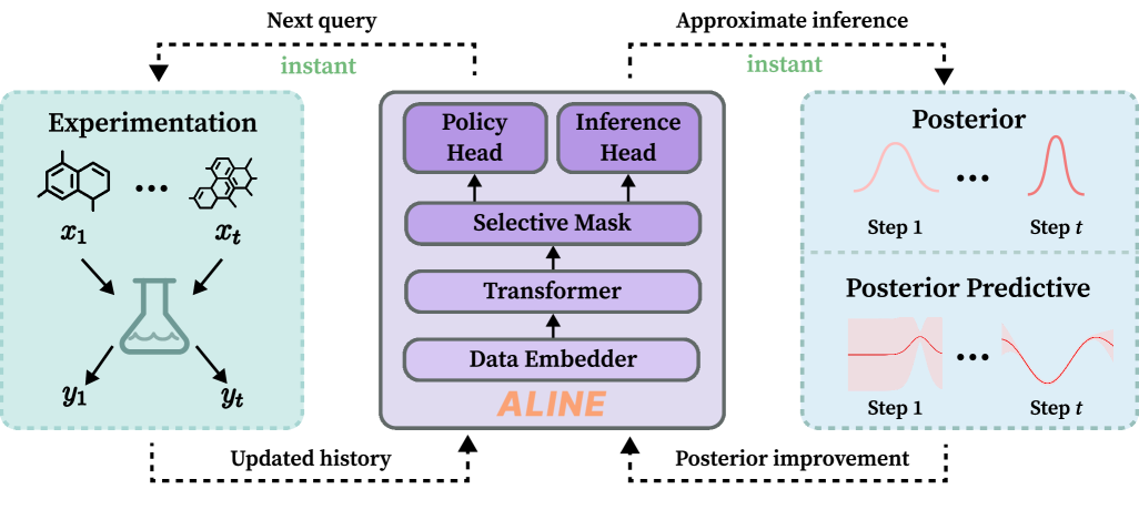
Figure 1: Conceptual workflow of Aline, demonstrating its capability to sequentially query informative data points and perform rapid posterior or predictive inference based on the gathered data.

To achieve both instant, informative querying and accurate inference, we propose to jointly learn an amortized inference model $q_{\phi}$ and an acquisition policy $\pi_{\psi}$ within a single, integrated architecture. Given the accumulated data history $\mathcal{D}_{t-1}$ and a specific target $\xi\in\Xi$, the policy $\pi_{\psi}$ selects the next query $x_{t}$ designed to be most informative for that target. Subsequently, the new data point $(x_{t},y_{t})$ is observed, and the inference model $q_{\phi}$ updates its estimate of the corresponding posterior or posterior predictive distribution. A conceptual workflow of Aline is illustrated in Figure˜1. In the remainder of this section, we detail the objectives for training the inference network $q_{\phi}$ (Section˜3.1) and the acquisition policy $\pi_{\psi}$ (Section˜3.2), discuss their practical implementation (Section˜3.3), and describe the unified model architecture (Section˜3.4).

3.1 Amortized inference

We use the inference network $q_{\phi}$ to provide accurate approximations of the true Bayesian posterior $p(\theta\,|\,\mathcal{D}_{T})$ or posterior predictive distributions $p({y}^{\star}\,|\,x^{\star},\mathcal{D}_{T})$, given the acquired data $\mathcal{D}_{T}$. We train $q_{\phi}$ via maximum-likelihood (Eq. 1). Specifically, for parameter targets $\xi=\xi_{S}^{\theta}$, our objective is:

$$\textstyle\mathcal{L}_{S}^{\theta}(\phi)=-\mathbb{E}_{p(\theta)p(\mathcal{D}_{T}\,|\,\theta)}\left[\log q_{\phi}(\theta_{S}\,|\,\mathcal{D}_{T})\right]=-\mathbb{E}_{p(\theta)p(\mathcal{D}_{T}\,|\,\theta)}\left[\sum_{l\in S}\log q_{\phi}(\theta_{l}\,|\,\mathcal{D}_{T})\right],$$ (5)

where we adopt a diagonal or mean field approximation, where the joint distribution is obtained as a product of marginals $q_{\phi}(\theta_{S}\,|\,\mathcal{D}_{T})=\prod_{l\in S}q_{\phi}(\theta_{l}\,|\,\mathcal{D}_{T})$. Analogously, for predictive targets $\xi=\xi_{p_{\star}}^{{y}^{\star}}$, we assume a factorized likelihood over targets sampled from the target input distribution $p_{\star}(x^{\star})$:

$$\textstyle\mathcal{L}^{{y}^{\star}}_{p_{\star}}(\phi)=-\mathbb{E}_{p(\theta)p(\mathcal{D}_{T}\,|\,\theta)p_{\star}(x^{\star}_{1:M})p({y}^{\star}_{1:M}\,|\,x^{\star}_{1:M},\theta)}\left[\sum_{m=1}^{M}\log q_{\phi}({y}^{\star}_{m}\,|\,x^{\star}_{m},\mathcal{D}_{T})\right].$$ (6)

The factorized form of these training objectives is a common scalable choice in the neural process literature (Garnelo et al., 2018a, ; Müller et al.,, 2022; Nguyen and Grover,, 2022; Chang et al.,, 2025) and more flexible than it might seem, as conditional marginal distributions can be extended to represent full joints autoregressively (Nguyen and Grover,, 2022; Bruinsma et al.,, 2023; Chang et al.,, 2025). For simplicity and tractability, within the scope of this paper we focus on the marginals, leaving the autoregressive extension to future work. Eqs. 5 and 6 form the basis for training the inference component $q_{\phi}$. Optimizing them minimizes the Kullback-Leibler (KL) divergence between the true target distributions (posterior or predictive) defined by the underlying generative process and the model’s approximations $q_{\phi}$ (Müller et al.,, 2022). Learning an accurate $q_{\phi}$ is crucial as it not only determines the quality of the final inference output but also serves as the basis for guiding the data acquisition policy, as we see next.

3.2 Amortized data acquisition

The quality of inference from $q_{\phi}$ depends critically on the informativeness of the acquired dataset $\mathcal{D}_{T}$. The acquisition policy $\pi_{\psi}$ is thus responsible for actively selecting a sequence of query-data pairs $(x_{t},y_{t})$ to maximize the information gained about a specific target $\xi$.

When targeting parameters $\theta_{S}$ (i.e., $\xi=\xi^{\theta}_{S}$), the objective is the total Expected Information Gain ($\text{sEIG}_{\theta_{S}}$) about $\theta_{S}$ over the $T$-step trajectory generated by $\pi_{\psi}$ (see Eq. 3):

$$\text{sEIG}_{\theta_{S}}(\psi)=\mathbb{E}_{p(\theta)p(\mathcal{D}_{T}\,|\,\pi_{\psi},\theta)}\left[\log p(\theta_{S}\,|\,\mathcal{D}_{T})\right]+H[p(\theta_{S})].$$ (7)

For completeness, we include a derivation of $\text{sEIG}_{\theta_{S}}$ in Section˜A.1 which is analogous to that of sEIG in (Foster et al.,, 2021). Directly optimizing sEIG is generally intractable due to its reliance on the unknown true posterior $p(\theta_{S}\,|\,\mathcal{D}_{T})$. We circumvent this by substituting $p(\theta_{S}\,|\,\mathcal{D}_{T})$ with its approximation $q_{\phi}(\theta_{S}\,|\,\mathcal{D}_{T})$ (from Eq. 5), yielding the tractable objective $\mathcal{J}^{\theta}_{S}$ for training $\pi_{\psi}$:

$$\textstyle\mathcal{J}_{S}^{\theta}(\psi):=\mathbb{E}_{p(\theta)p(\mathcal{D}_{T}\,|\,\pi_{\psi},\theta)}\left[\sum_{l\in S}\log q_{\phi}(\theta_{l}\,|\,\mathcal{D}_{T})\right]+H[p(\theta_{S})].$$ (8)

The inference objective (Eq. 5) and this policy objective are thus coupled: $\mathcal{L}_{S}^{\theta}(\phi)$ depends on data $\mathcal{D}_{T}$ acquired through $\pi_{\psi}$, and $\mathcal{J}_{S}^{\theta}(\psi)$ depends on the inference network $q_{\phi}$.

Similarly, when targeting predictions for $\xi=\xi_{p_{\star}}^{{y}^{\star}}$, we aim to maximize information about $p({y}^{\star}\,|\,x^{\star},\mathcal{D}_{T})$ for $x^{\star}\sim p_{\star}(x^{\star})$. We extend the Expected Predictive Information Gain (EPIG) framework (Smith et al.,, 2023) to the amortized sequential setting, defining the total sEPIG:

Proposition 1.

The total expected predictive information gain for a design policy $\pi_{\psi}$ over a data trajectory of length $T$ is:

$$\text{sEPIG}(\psi) :=\mathbb{E}_{p_{\star}(x^{\star})p(\mathcal{D}\,|\,\pi_{\psi})}[H[p({y}^{\star}\,|\,x^{\star})]-H[p({y}^{\star}\,|\,x^{\star},\mathcal{D}_{T})]]$$

$$\,=\mathbb{E}_{p(\theta)p(\mathcal{D}_{T}\,|\,\pi_{\psi},\theta)p_{\star}(x^{\star})p({y}^{\star}\,|\,x^{\star},\theta)}\left[\log p({y}^{\star}\,|\,x^{\star},\mathcal{D}_{T})\right]+\mathbb{E}_{p_{\star}(x^{\star})}[H[p({y}^{\star}\,|\,x^{\star})]].$$

This result adapts Theorem 1 in (Foster et al.,, 2021) for the predictive case (see Section˜A.2 for proof) and, unlike single-step EPIG (Eq. 4), considers the entire trajectory $\mathcal{D}_{T}$ given the policy $\pi_{\psi}$.

Now, similar to Eq. 8, we use the inference network $q_{\phi}({y}^{\star}\,|\,x^{\star},\mathcal{D}_{T})$ to replace the true posterior predictive distribution $p({y}^{\star}\,|\,x^{\star},\mathcal{D}_{T})$ in Proposition˜1 to obtain our active learning objective:

$$\mathcal{J}^{{y}^{\star}}_{p_{\star}}(\psi):=\mathbb{E}_{p(\theta)p(\mathcal{D}_{T}\,|\,\pi_{\psi},\theta)p_{\star}(x^{\star})p({y}^{\star}\,|\,x^{\star},\theta)}\left[\log q_{\phi}({y}^{\star}\,|\,x^{\star},\mathcal{D}_{T})\right]+\mathbb{E}_{p_{\star}(x^{\star})}[H[p({y}^{\star}\,|\,x^{\star})]].$$ (9)

Finally, the following proposition proves that our acquisition objectives, $\mathcal{J}_{S}^{\theta}$ and $\mathcal{J}_{p_{\star}}^{{y}^{\star}}$, are variational lower bounds on the true total information gains ($\text{sEIG}_{\theta_{S}}$ and sEPIG, respectively), making them principled tractable objectives for our goal. The proof is given in Section˜A.3.

Proposition 2.

Let the policy $\pi_{\psi}$ generate the trajectory $\mathcal{D}_{T}$. With $q_{\phi}(\theta_{S}\,|\,\mathcal{D_{T}})$ approximating $p(\theta_{S}\,|\,\mathcal{D_{T}})$, and $q_{\phi}({y}^{\star}\,|\,x^{\star},\mathcal{D}_{T})$ approximating $p({y}^{\star}\,|\,x^{\star},\mathcal{D}_{T})$, we have $\mathcal{J}_{S}^{\theta}(\psi)\leq\text{sEIG}_{\theta_{S}}(\psi)$ and $\mathcal{J}_{p_{\star}}^{{y}^{\star}}(\psi)\leq\text{sEPIG}(\psi)$. Moreover,

$$\text{sEIG}_{\theta_{S}}(\psi)-\mathcal{J}_{S}^{\theta}(\psi) =\mathbb{E}_{p(\mathcal{D}_{T}\,|\,\pi_{\psi})}[\text{KL}(p(\theta_{S}\,|\,\mathcal{D}_{T})||q_{\phi}(\theta_{S}\,|\,\mathcal{D}_{T}))],\quad\text{and}$$

$$\text{sEPIG}(\psi)-\mathcal{J}^{{y}^{\star}}_{p_{\star}}(\psi) =\mathbb{E}_{p_{\star}(x^{\star})p(\mathcal{D}_{T}\,|\,\pi_{\psi})}[\text{KL}(p({y}^{\star}\,|\,x^{\star},\mathcal{D}_{T})||q_{\phi}({y}^{\star}\,|\,x^{\star},\mathcal{D}_{T}))].$$

This principle of using approximate posterior (or predictive) distributions to bound information gain is foundational in Bayesian experimental design (e.g., (Foster et al.,, 2019)) and has been extended to sequential amortized settings (e.g., the sCEE bound in (Blau et al.,, 2022)). Maximizing these $\mathcal{J}$ objectives thus encourages policies that increase information about the targets. The tightness of these bounds is governed by the expected KL divergence between the true quantities and their approximation, with a more accurate $q_{\phi}$ leading to tighter bounds and a more effective training signal for the policy.

Data acquisition objective for Aline.

To handle any target $\xi\in\Xi$ from a user-specified set, we unify the previously defined acquisition objectives. We define $\mathcal{J}(\psi,\xi)$ based on the type of target $\xi$:

$$\mathcal{J}(\psi,\xi)=\begin{cases}\mathcal{J}^{\theta}_{S}(\psi),&\text{if }\xi=\xi^{\theta}_{S}\\ \mathcal{J}_{p_{\star}}^{{y}^{\star}}(\psi),&\text{if }\xi=\xi_{p_{\star}}^{{y}^{\star}}.\end{cases}$$

The final objective for learning the policy network $\pi_{\psi}$, denoted as $\mathcal{J}^{\Xi}$, is the expectation of $\mathcal{J}(\psi,\xi)$ taken over the distribution of possible target specifiers $p(\xi)$: $\mathcal{J}^{\Xi}(\psi)=\mathbb{E}_{\xi\sim p(\xi)}[\mathcal{J}(\psi,\xi)]$.

3.3 Training methodology for Aline

The policy and inference networks, $\pi_{\psi}$ and $q_{\phi}$, in Aline are trained jointly. Training $\pi_{\psi}$ for sequential data acquisition over a $T$-step horizon is naturally framed as a reinforcement learning (RL) problem.

Policy network training ($\pi_{\psi}$).

To guide the policy, we employ a dense, per-step reward signal $R_{t}$ rather than relying on a sparse reward at the end of the trajectory. This approach, common in amortized experimental design (Blau et al.,, 2022, 2023; Huang et al.,, 2025), helps stabilize and accelerate learning. The reward $R_{t}$ quantifies the immediate improvement in the inference quality provided by $q_{\phi}$ upon observing a new data point $(x_{t},y_{t})$, specifically concerning the current target $\xi$. It is defined based on the one-step change in the log-probabilities from our acquisition objectives (Eqs. 8 and 9):

$$R_{t}(\xi)=\begin{cases}\frac{1}{|S|}\sum_{l\in S}(\log q_{\phi}(\theta_{l}\,|\,\mathcal{D}_{t})-\log q_{\phi}(\theta_{l}\,|\,\mathcal{D}_{t-1})),&\text{if }\xi=\xi^{\theta}_{S}\\ \frac{1}{M}\sum_{m=1}^{M}(\log q_{\phi}({y}^{\star}_{m}\,|\,x^{\star}_{m},\mathcal{D}_{t})-\log q_{\phi}({y}^{\star}_{m}\,|\,x^{\star}_{m},\mathcal{D}_{t-1})),&\text{if }\xi=\xi^{{y}^{\star}}_{p_{\star}}.\end{cases}$$ (10)

As per common practice, for gradient stabilization we take averages (not sums) over predictions, which amounts to a constant relative rescaling of our objectives. The policy $\pi_{\psi}$ is then trained using a policy gradient (PG) algorithm with per-episode loss:

$$\textstyle\mathcal{L}_{\text{PG}}(\psi)=-\sum_{t=1}^{T}\gamma^{t}R_{t}(\xi)\log\pi_{\psi}(x_{t}|\mathcal{D}_{t-1},\xi),$$ (11)

which maximizes the expected cumulative $\gamma$-discounted reward over trajectories (Sutton et al.,, 1999).

Inference network training ($q_{\phi}$).

For the per-step rewards $R_{t}$ to be meaningful, the inference network $q_{\phi}$ must provide accurate estimates of posteriors or predictive distributions at each intermediate step $t$ of the acquisition sequence, not just at the final step $T$. Consequently, the practical training objective for $q_{\phi}$, denoted $\mathcal{L}_{\text{NLL}}(\phi)$, encourages this step-wise accuracy. In practice, training proceeds in episodes. For each episode: (1) A ground truth parameter set $\theta$ is sampled from the prior $p(\theta)$. (2) A target specifier $\xi$ is sampled from $p(\xi)$. (3) If the target is predictive ($\xi=\xi_{p_{*}}^{{y}^{\star}}$), $M$ target input locations $\{x^{\star}_{m}\}_{m=1}^{M}$ are sampled from $p_{\star}(x^{\star})$, and their corresponding true outcomes $\{{y}^{\star}_{m}\}_{m=1}^{M}$ are simulated using $\theta$, similarly as (Smith et al.,, 2023). The negative log-likelihood loss $\mathcal{L}_{\text{NLL}}(\phi)$ for $q_{\phi}$ in an episode is then computed by averaging over the $T$ acquisition steps and predictions, using the Monte Carlo estimates of the objectives defined in Eqs. 5 and 6:

$$\mathcal{L}_{\text{NLL}}(\phi)\approx\begin{cases}-\frac{1}{T}\frac{1}{|S|}\sum_{t=1}^{T}\sum_{l\in S}\log q(\theta_{l}\,|\,\mathcal{D}_{t}),&\text{if }\xi=\xi^{\theta}_{S}\\ -\frac{1}{T}\frac{1}{M}\sum_{t=1}^{T}\sum_{m=1}^{M}\log q({y}^{\star}_{m}\,|\,x^{\star}_{m},\mathcal{D}_{t}),&\text{if }\xi=\xi^{{y}^{\star}}_{p_{\star}}.\\ \end{cases}$$ (12)

Joint training.

To ensure $q_{\phi}$ provides a reasonable reward signal early in training, we employ an initial warm-up phase where only $q_{\phi}$ is trained, with data acquisition $(x_{t},y_{t})$ guided by random actions instead of $\pi_{\psi}$. After the warm-up, $q_{\phi}$ and $\pi_{\psi}$ are trained jointly. A detailed step-by-step training algorithm is provided in Section˜B.1.

3.4 Architecture

Aline employs a single, integrated neural architecture based on Transformer Neural Process (TNP) (Nguyen and Grover,, 2022; Chang et al.,, 2025), to concurrently manage historical observations, propose future queries, and condition predictions on specific, potentially varying, inference objectives. An overview of Aline’s architecture is provided in Figure˜A1.

The model inputs are structured into three sets. Following standard TNP-based architecture, the context set $\mathcal{D}_{t}=\{(x_{i},y_{i})\}_{i=1}^{t}$ comprises the history of observations, and the target set $\mathcal{T}$ contains the specific target specifier $\xi$. To facilitate active data acquisition, we incorporate a query set $\mathcal{Q}=\{x^{\text{q}}_{n}\}_{n=1}^{N}$ of candidate points. In this paper, we focus on a discrete pool-based setting for consistency, though it can be straightforwardly extended to continuous design spaces (e.g., (Schulman et al.,, 2015)). Details regarding the embeddings of these inputs are provided in Section˜B.2.

Standard transformer attention mechanisms process these embedded representations. Self-attention operates within the context set, capturing dependencies within $\mathcal{D}_{t}$. Both the query and target set then employ cross-attention to attend to the processed context set representations. To enable the policy $\pi_{\psi}$ to dynamically adapt its acquisition strategy based on the specific inference goal $\xi$, we introduce an additional query-target cross-attention mechanism to allow the query candidates to directly attend to the target set. This allows the evaluation of each candidate $x^{\text{q}}_{n}$ to be informed by its relevance to the different potential targets $\xi$. Examples of the attention mask are shown in Figure˜A2.

Finally, two specialized output heads operate on these processed representations. The inference head ($q_{\phi}$), following ACE (Chang et al.,, 2025), uses a Gaussian mixture to parameterize the approximate posteriors and posterior predictives. The acquisition head ($\pi_{\psi}$) generates a policy over the query set $\pi_{\psi}(x_{t+1}|\mathcal{D}_{t})$, drawing on principles from policy-based design methods (Huang et al.,, 2025; Maraval et al.,, 2024). This novel combination within a TNP framework allows Aline to effectively integrate established components for inference and acquisition with a new mechanism for adaptive goal-oriented querying.

4 Related work

A major family of ABI methods is Neural Processes (NPs) (Garnelo et al., 2018b, ; Garnelo et al., 2018a, ), which learn a mapping from observed context data points to a predictive distribution for new target points. Early NPs often employed MLP-based encoders (Garnelo et al., 2018b, ; Garnelo et al., 2018a, ; Huang et al., 2023b, ; Bruinsma et al.,, 2023), while more recent works utilize more advanced attention and transformer architectures (Kim et al.,, 2019; Nguyen and Grover,, 2022; Müller et al.,, 2022; Feng et al.,, 2023, 2024; Ashman et al., 2024b, ; Ashman et al., 2024a, ). Complementary to NPs, methods within simulation-based inference (Cranmer et al.,, 2020) focus on amortizing the posterior distribution (Papamakarios and Murray,, 2016; Lueckmann et al.,, 2017; Greenberg et al.,, 2019; Radev et al., 2023b, ; Mittal et al.,, 2025; Zammit-Mangion et al.,, 2024). More recently, methods for amortizing both the posterior and posterior predictive distributions have been proposed (Gloeckler et al.,, 2024; Radev et al., 2023a, ; Chang et al.,, 2025). Specifically, ACE (Chang et al.,, 2025) shows how to flexibly condition on diverse user-specified inference targets, a method Aline incorporates for its own flexible inference capabilities. Building on this principle of goal-directed adaptability, Aline advances it by integrating a learned policy that dynamically tailors the data acquisition strategy to such specified objectives.

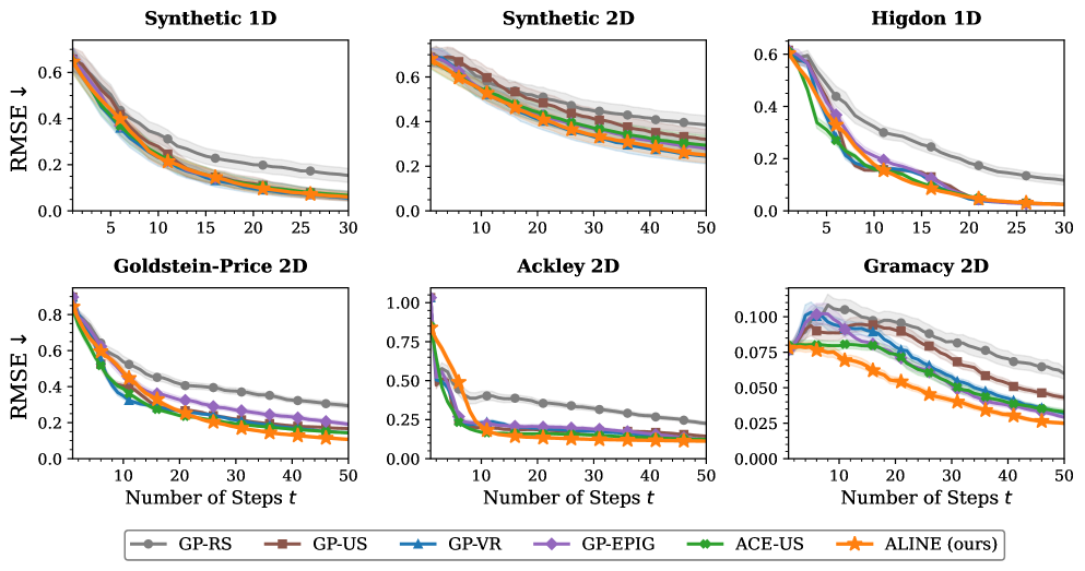
Figure 2: Predictive performance on active learning benchmark functions (RMSE $\downarrow$). Results show the mean and 95% confidence interval (CI) across 100 runs.

Existing amortized BED or BAL methods (Foster et al.,, 2021; Ivanova et al.,, 2021; Blau et al.,, 2022; Li et al.,, 2025) that learn an offline design policy do not provide real-time estimates of the posterior, unlike Aline. An exception to this is the recent work of Blau et al., (2023), which uses a variational posterior bound to provide amortized posterior inference via a separate proposal network. Compared to their method, Aline uses a single, unified architecture where the same model performs amortized inference for both posterior and posterior predictive distributions, and learns the flexible acquisition policy. Recently, transformer-based models have been explored in various amortized sequential decision-making settings, including decision-aware BED (Huang et al.,, 2025), Bayesian optimization (BO) (Maraval et al.,, 2024), multi-objective BO (Hung et al.,, 2025), and preferential BO (Zhang et al.,, 2025).

5 Experiments

We now empirically evaluate Aline’s performance in different active data acquisition and amortized inference tasks. We begin with the active learning task in Section˜5.1, where we want to efficiently minimize the uncertainty over an unknown function by querying $T$ data points. Then, we test Aline’s policy on standard BED benchmarks in Section˜5.2. Finally, in Section˜5.3, we demonstrate the benefit of Aline’s flexible targeting feature in a psychometric modeling task (Wichmann and Hill,, 2001). The code to reproduce our experiments is available at: https://github.com/huangdaolang/aline.

5.1 Active learning for regression and hyperparameter inference

For the active learning task, Aline is trained on a diverse collection of fully synthetic functions drawn from Gaussian Process (GP) (Rasmussen and Williams,, 2006) priors (see Section˜C.1.1 for details). We evaluate Aline’s performance under both in-distribution and out-of-distribution settings. For the in-distribution setting, Aline is evaluated on synthetic functions sampled from the same GP prior that is used during training. In the out-of-distribution setting, we evaluate Aline on benchmark functions (Higdon, Goldstein-Price, Ackley, and Gramacy) unseen during training, to assess generalization beyond the training regime. We compare Aline against non-amortized GP models equipped with standard acquisition functions such as Uncertainty Sampling (GP-US), Variance Reduction (GP-VR) (Yu et al.,, 2006), EPIG (GP-EPIG) (Smith et al.,, 2023), and Random Sampling (GP-RS). Additionally, we include an amortized inference baseline, the Amortized Conditioning Engine (ACE) (Chang et al.,, 2025), paired with Uncertainty Sampling (ACE-US), to specifically evaluate the advantage of Aline’s learned acquisition policy over using a standard acquisition function with an amortized inference model. The performance metric is the root mean squared error (RMSE) of the predictions on a held-out test set.

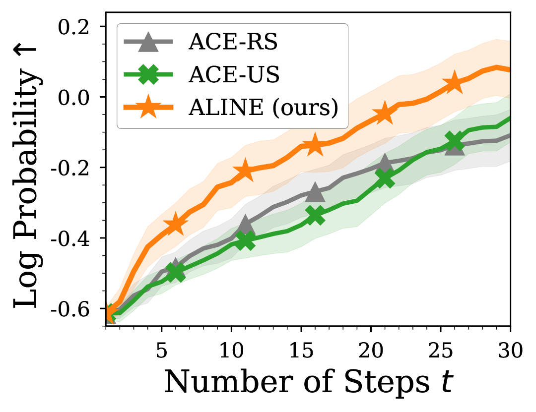
Figure 3: Hyperparameter inference performance on synthetic GP functions.

Results for the active learning task in Figure˜2 show that Aline performs comparably to the best-performing GP-based methods for the in-distribution setting. Importantly, for the out-of-distribution setting, Aline outperforms the baselines in 3 out of the 4 benchmark functions. These results highlight the advantage of Aline’s end-to-end learning strategy, which obviates the need for kernel specification using GPs or explicit acquisition function selection. Further evaluations on additional benchmark functions (Gramacy 1D, Branin, Three Hump Camel), visualizations of Aline’s sequential querying strategy with corresponding predictive updates, and a comparison of average inference times are provided in Section˜D.1.

Additionally, for the in-distribution setting, we test Aline’s capability to infer the underlying GP’s hyperparameters—without retraining, by leveraging Aline’s flexible target specification at runtime. For baselines, we use ACE-US and ACE-RS, since ACE (Chang et al.,, 2025) is also capable of posterior estimation. Figure˜3 shows that Aline yields higher log probabilities of the true parameter value under the estimated posterior at each step compared to the baselines. This is due to the ability to flexibly switch Aline’s acquisition strategy to parameter inference, unlike other active learning methods. We also visualize the obtained posteriors in Section˜D.1.

5.2 Benchmarking on Bayesian experimental design tasks

We test Aline on two classical BED tasks: Location Finding (Sheng and Hu,, 2004) and Constant Elasticity of Substitution (CES) (Arrow et al.,, 1961), with two- and six-dimensional design space, respectively. As baselines, we include a random design policy, a gradient-based method with variational Prior Contrastive Estimation (VPCE) (Foster et al.,, 2020), and two amortized BED methods: Deep Adaptive Design (DAD) (Foster et al.,, 2021) and RL-BOED (Blau et al.,, 2022). Details of the tasks and the baselines are provided in Section˜C.2.

To evaluate performance, we compute a lower bound of the total EIG, namely the sequential Prior Contrastive Estimation lower bound (Foster et al.,, 2021). As shown in Table˜2, Aline surpasses all the baselines in the Location Finding task and achieves performance comparable to RL-BOED in the CES task. Notably, Aline’s training time is reduced as its reward is based on the internal posterior improvement and does not require a large number of contrastive samples to estimate sEIG. While Aline’s deployment time is slightly higher than MLP-based amortized methods due to the computational cost of its transformer architecture, it remains orders of magnitude faster than non-amortized approaches like VPCE. Visualizations of Aline’s inferred posterior distributions are provided in Section˜D.2.

Table 2: Results on BED benchmarks. For the EIG lower bound, we report the mean $\pm$ 95% CI across 2000 runs (200 for VPCE). For deployment time, we use the mean $\pm$ 95% CI from 20 runs.

	Location Finding			Constant Elasticity of Substitution
	EIG lower bound ($\uparrow$)	Training time (h)	Deployment time (s)	EIG lower bound ($\uparrow$)	Training time (h)	Deployment time (s)
Random	5.17$\pm$0.05	N/A	N/A	9.05$\pm$0.26	N/A	N/A
VPCE (Foster et al.,, 2020)	5.25$\pm$0.22	N/A	146.59$\pm$0.09	9.40$\pm$0.27	N/A	788.90$\pm$1.03
DAD (Foster et al.,, 2021)	7.33$\pm$0.06	7.24	0.0001$\pm$0.00	10.77$\pm$0.15	13.70	0.0001$\pm$0.00
RL-BOED (Blau et al.,, 2022)	7.70$\pm$0.06	63.29	0.0003$\pm$0.00	14.60$\pm$0.10	67.28	0.0004$\pm$0.00
Aline (ours)	8.91$\pm$0.04	21.20	0.03$\pm$0.00	14.37$\pm$0.08	13.29	0.04$\pm$0.00

5.3 Psychometric model

Our final experiment involves the psychometric modeling task (Wichmann and Hill,, 2001)—a fundamental scenario in behavioral sciences, from neuroscience to clinical settings (Gilaie-Dotan et al.,, 2013; Powers et al.,, 2017; Xu et al.,, 2024), where the goal is to infer parameters governing an observer’s responses to varying stimulus intensities. The psychometric function used here is characterized by four parameters: threshold, slope, guess rate, and lapse rate; see Section˜C.3.1 for details. Different research questions in psychophysics necessitate focusing on different parameter subsets. For instance, studies on perceptual sensitivity primarily target precise estimation of threshold and slope, while investigations into response biases or attentional phenomena might focus on the guess and lapse rates. This is where Aline’s unique flexible querying strategy can be used to target specific parameter subsets of interest.

We compare Aline with two established adaptive psychophysical methods: QUEST+ (Watson,, 2017), which targets all parameters simultaneously, and Psi-marginal (Prins,, 2013), which can marginalize over nuisance parameters to focus on a specified subset, a non-amortized gold-standard method for flexible acquisition. We evaluate scenarios targeting either the threshold and slope parameters or the guess and lapse rates. Details of the baselines and the experimental setup are in Section˜C.3.2.

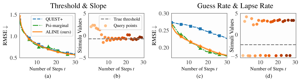
Figure 4: Results on psychometric model. RMSE (mean $\pm$ 95% CI) when targeting (a) threshold & slope and (c) guess & lapse rates, with Aline’s corresponding query strategies shown in (b) and (d).

Figure˜4 shows the results. When targeting threshold and slope (Figure˜4a), which are generally easier to infer, Aline achieves results comparable to baselines. When targeting guess and lapse rates (Figure˜4c), QUEST+ performs sub-optimally as its experimental design strategy is dominated by the more readily estimable threshold and slope parameters. In contrast, both Psi-marginal and Aline lead to significantly better inference than QUEST+ when explicitly targeting guess and lapse rates. Moreover, Aline offers a $10\times$ speedup over these non-amortized methods (See Appendix˜D). We also visualize the query strategies adopted by Aline in the two cases: when targeting threshold and slope (Figure˜4b), stimuli are concentrated near the estimated threshold. Conversely, when targeting guess and lapse rates (Figure˜4d), Aline appropriately selects ‘easy’ stimuli at extreme values where mistakes can be more readily attributed to random behavior (governed by lapses and guesses) rather than the discriminative ability of the subject (governed by threshold and slope).

6 Conclusion

We introduced Aline, a unified amortized framework that seamlessly integrates active data acquisition with Bayesian inference. Aline dynamically adapts its strategy to target selected inference goals, offering a flexible and efficient solution for Bayesian inference and active data acquisition.

Limitations & future work.

Currently, Aline operates with pre-defined, fixed priors, necessitating re-training for different prior specifications. Future work could explore prior amortization (Chang et al.,, 2025; Whittle et al.,, 2025), to allow for dynamic prior conditioning. As Aline estimates marginal posteriors, extending this to joint posterior estimation, potentially via autoregressive modeling (Bruinsma et al.,, 2023), is a promising direction. Note that, at deployment, we may encounter observations that differ substantially from the training data, leading to degradation in performance. This issue can potentially be tackled by combining Aline with robust approaches such as (Forster et al.,, 2025; Huang et al., 2023a, ). Lastly, Aline’s current architecture is tailored to fixed input dimensionalities and discrete design spaces, a common practice with TNPs (Nguyen and Grover,, 2022; Maraval et al.,, 2024; Zhang et al.,, 2025; Huang et al.,, 2025). Generalizing Aline to be dimension-agnostic (Lee et al.,, 2025) and to support continuous experimental designs (Schulman et al.,, 2015) are valuable avenues for future research.

Acknowledgements

DH, LA and SK were supported by the Research Council of Finland (Flagship programme: Finnish Center for Artificial Intelligence FCAI). LA was also supported by Research Council of Finland grants 358980 and 356498. SK was also supported by the UKRI Turing AI World-Leading Researcher Fellowship, [EP/W002973/1]. AB was supported by the Research Council of Finland grant no. 362534. The authors wish to thank Aalto Science-IT project, and CSC–IT Center for Science, Finland, for the computational and data storage resources provided.

Appendix

The appendix is organized as follows:

• In Appendix˜A, we provide detailed derivations and proofs for the theoretical claims made regarding information gain and variational bounds.

• In Appendix˜B, we present the complete training algorithm and the specifics of the Aline model.

• In Appendix˜C, we provide comprehensive details for each experimental setup, including task descriptions and baseline implementations.

• In Appendix˜D, we present additional experimental results, including further visualizations, performance on more benchmarks, and analyses of inference times.

• In Appendix˜E, we provide an overview of the computational resources and software dependencies for this work.

Appendix A Proofs of theoretical results

A.1 Derivation of total EIG for $\theta_{S}$

Following Eq. 3, we can write the expression for the total expected information gain sEIG${}_{\theta_{S}}$ about a parameter subset $\theta_{S}\subseteq\theta$ given data $\mathcal{D}_{T}$ generated under policy $\pi_{\psi}$ as:

$$\text{sEIG}_{\theta_{S}}(\psi)=H[p(\theta_{S})]+\underbrace{\mathbb{E}_{p(\theta_{S},\mathcal{D}_{T}\,|\,\pi_{\psi})}[\log p(\theta_{S}\,|\,\mathcal{D}_{T})]}_{E_{1}},$$ (A1)

where $p(\theta_{S})$ is the marginal prior for $\theta_{S}$, and $p(\theta_{S},\mathcal{D}_{T}\,|\,\pi_{\psi})$ is the joint distribution of $\theta_{S}$ and $\mathcal{D}_{T}$ under $\pi_{\psi}$. Now, let $\theta_{R}=\theta\setminus\theta_{S}$ be the remaining component of $\theta$ not included in $\theta_{S}$. Then, we can express $E_{1}$ from Eq. A1 as

$$E_{1} =\int\log p(\theta_{S}\,|\,\mathcal{D}_{T})p(\theta_{S},\mathcal{D}_{T}\,|\,\pi_{\psi})\text{d}\theta_{S}$$

$$=\int\log p(\theta_{S}\,|\,\mathcal{D}_{T})\left[\int p(\theta_{S},\theta_{R},\mathcal{D}_{T}\,|\,\pi_{\psi})\text{d}\theta_{R}\right]\text{d}\theta_{S}$$

$$=\int\log p(\theta_{S}\,|\,\mathcal{D}_{T})\int p(\theta,\mathcal{D}_{T}\,|\,\pi_{\psi})\text{d}\theta$$

$$=\mathbb{E}_{p(\theta,\mathcal{D}_{T}\,|\,\pi_{\psi})}[\log p(\theta_{S}\,|\,\mathcal{D}_{T})].$$ (A2)

Plugging the above expression in Eq. A1 and noting that $p(\theta,\mathcal{D}_{T}\,|\,\pi_{\psi})=p(\theta)p(\mathcal{D}_{T}\,|\,\theta,\pi_{\psi})$, we arrive at the expression for sEIG${}_{\theta_{S}}$ in Eq. 7.

A.2 Proof of Proposition 1

Proposition (Proposition 1).

The total expected predictive information gain for a design policy $\pi_{\psi}$ over a data trajectory of length $T$ is:

$$\text{sEPIG}(\psi) :=\mathbb{E}_{p_{\star}(x^{\star})p(\mathcal{D}\,|\,\pi_{\psi})}[\text{H}[p({y}^{\star}\,|\,x^{\star})]-\text{H}[p({y}^{\star}\,|\,x^{\star},\mathcal{D}_{T})]]$$

$$\,=\mathbb{E}_{p(\theta)p(\mathcal{D}_{T}\,|\,\pi_{\psi},\theta)p_{\star}(x^{\star})p({y}^{\star}\,|\,x^{\star},\theta)}\left[\log p({y}^{\star}\,|\,x^{\star},\mathcal{D}_{T})\right]+\mathbb{E}_{p_{\star}(x^{\star})}[H[p({y}^{\star}\,|\,x^{\star})]].$$

Proof.

Let $p_{\star}(x^{\star})$ be the target distribution over inputs $x^{\star}$ for which we want to improve predictive performance. Let ${y}^{\star}$ be the corresponding target output. The single-step EPIG for acquiring data $(x,y)$ measures the expected reduction in uncertainty (entropy) about ${y}^{\star}$ for a random target $x^{\star}\sim p_{\star}(x^{\star})$:

$$\text{EPIG}(x)=\mathbb{E}_{p_{\star}(x^{\star})p(y\,|\,x)}[H[p({y}^{\star}\,|\,x^{\star})]-H[p({y}^{\star}\,|\,x^{\star},x,y)]].$$

Following Theorem 1 in (Foster et al.,, 2021), the total EPIG, is the total expected reduction in predictive entropy from the initial prediction $p({y}^{\star}\,|\,x^{\star})$ to the final prediction based on the full history $p({y}^{\star}\,|\,x^{\star},\mathcal{D}_{T})$:

$$\text{sEPIG}(\psi) =\mathbb{E}_{p_{\star}(x^{\star})p(\mathcal{D}_{T}\,|\,\pi_{\psi})}[H[p({y}^{\star}\,|\,x^{\star})]-H[p({y}^{\star}\,|\,x^{\star},\mathcal{D}_{T})]]$$ (A3)

$$=\mathbb{E}_{p_{\star}(x^{\star})p(\mathcal{D}_{T}\,|\,\pi_{\psi})}[\mathbb{E}_{p({y}^{\star}\,|\,x^{\star},\mathcal{D}_{T})}[\log p({y}^{\star}\,|\,x^{\star},\mathcal{D}_{T})]]+\mathbb{E}_{p_{\star}(x^{\star})}[H[p({y}^{\star}\,|\,x^{\star})]]$$ (A4)

$$=\mathbb{E}_{p_{\star}(x^{\star})p(\mathcal{D}_{T},{y}^{\star}\,|\,\pi_{\psi},x^{\star})}[\log p({y}^{\star}\,|\,x^{\star},\mathcal{D}_{T})]+\mathbb{E}_{p_{\star}(x^{\star})}[H[p({y}^{\star}\,|\,x^{\star})]].$$ (A5)

Here, Eq. A3 follows from conditioning EPIG on the entire trajectory $\mathcal{D}_{T}$ instead of a single data point $y$, Eq. A4 follows from the definition of entropy $H[\cdot]$, and Eq. A5 follows from noting that $p(\mathcal{D}_{T},{y}^{\star}\,|\,\pi_{\psi},x^{\star})=p(\mathcal{D}_{T}\,|\,\pi_{\psi})p({y}^{\star}\,|\,x^{\star},\mathcal{D}_{T})$. Next, we combine the expectations and express the joint distribution $p(\mathcal{D}_{T},{y}^{\star}\,|\,\pi_{\psi},x^{\star})=\int p(\theta)p(\mathcal{D}_{T}\,|\,\pi_{\psi},\theta)p({y}^{\star}\,|\,x^{\star},\theta)d\theta$, where, following (Smith et al.,, 2023), we assume conditional independence between $\mathcal{D}_{T}$ and ${y}^{\star}$ given $\theta$. This yields:

$$\text{sEPIG}(\psi)=\mathbb{E}_{p(\theta)p(\mathcal{D}_{T}\,|\,\pi_{\psi},\theta)p_{\star}(x^{\star})p({y}^{\star}\,|\,x^{\star},\theta)}\left[\log p({y}^{\star}\,|\,x^{\star},\mathcal{D}_{T})\right]+\mathbb{E}_{p_{\star}(x^{\star})}[H[p({y}^{\star}\,|\,x^{\star})]],$$

which completes our proof. ∎

A.3 Proof of Proposition 2

Proposition (Proposition 2).

Let the policy $\pi_{\psi}$ generate the trajectory $\mathcal{D}_{T}$. With $q_{\phi}(\theta_{S}\,|\,\mathcal{D_{T}})$ approximating $p(\theta_{S}\,|\,\mathcal{D_{T}})$, and $q_{\phi}({y}^{\star}\,|\,x^{\star},\mathcal{D}_{T})$ approximating $p({y}^{\star}\,|\,x^{\star},\mathcal{D}_{T})$, we have $\mathcal{J}_{S}^{\theta}(\psi)\leq\text{sEIG}_{\theta_{S}}(\psi)$ and $\mathcal{J}_{p_{\star}}^{{y}^{\star}}(\psi)\leq\text{sEPIG}(\psi)$. Moreover,

$$\text{sEIG}_{\theta_{S}}(\psi)-\mathcal{J}_{S}^{\theta}(\psi) =\mathbb{E}_{p(\mathcal{D}_{T}\,|\,\pi_{\psi})}[\text{KL}(p(\theta_{S}\,|\,\mathcal{D}_{T})||q_{\phi}(\theta_{S}\,|\,\mathcal{D}_{T}))],\quad\text{and}$$ (A6)

$$\text{sEPIG}(\psi)-\mathcal{J}^{{y}^{\star}}_{p_{\star}}(\psi) =\mathbb{E}_{p_{\star}(x^{\star})p(\mathcal{D}_{T}\,|\,\pi_{\psi})}[\text{KL}(p({y}^{\star}\,|\,x^{\star},\mathcal{D}_{T})||q_{\phi}({y}^{\star}\,|\,x^{\star},\mathcal{D}_{T}))].$$ (A7)

Proof.

Using the expressions for $\text{sEIG}_{\theta_{S}}$ and $\mathcal{J}_{S}^{\theta}$ from Eq. 7 and Eq. 8, respectively, and noting that $q_{\phi}(\theta_{S}\,|\,\mathcal{D}_{T})=\sum_{l\in S}q_{\phi}(\theta_{l}\,|\,\mathcal{D}_{T})$, we can write the expression for $\text{sEIG}_{\theta_{S}}(\psi)-\mathcal{J}_{S}^{\theta}(\psi)$ as:

$$\text{sEIG}_{\theta_{S}}(\psi)-\mathcal{J}_{S}^{\theta}(\psi) =\mathbb{E}_{p(\theta)p(\mathcal{D}_{T}\,|\,\pi_{\psi},\theta)}[\log p(\theta_{S}\,|\,\mathcal{D}_{T})]-\mathbb{E}_{p(\theta)p(\mathcal{D}_{T}\,|\,\pi_{\psi},\theta)}[\log q_{\phi}(\theta_{S}\,|\,\mathcal{D}_{T})]$$

$$=\mathbb{E}_{p(\mathcal{D}_{T},\theta\,|\,\pi_{\psi},\theta)}\left[\log\frac{p(\theta_{S}\,|\,\mathcal{D}_{T})}{q_{\phi}(\theta_{S}\,|\,\mathcal{D}_{T})}\right]$$ (A8)

$$=\mathbb{E}_{p(\mathcal{D}_{T},\theta_{S}\,|\,\pi_{\psi},\theta)}\left[\log\frac{p(\theta_{S}\,|\,\mathcal{D}_{T})}{q_{\phi}(\theta_{S}\,|\,\mathcal{D}_{T})}\right]$$ (A9)

$$=\mathbb{E}_{p(\mathcal{D}_{T}\,|\,\pi_{\psi})}\left[\mathbb{E}_{p(\theta_{S}\,|\,\mathcal{D}_{T})}\left[\log\frac{p(\theta_{S}\,|\,\mathcal{D}_{T})}{q_{\phi}(\theta_{S}\,|\,\mathcal{D}_{T})}\right]\right]$$ (A10)

$$=\mathbb{E}_{p(\mathcal{D}_{T}\,|\,\pi_{\psi})}[\text{KL}(p(\theta_{S}\,|\,\mathcal{D}_{T})||q_{\phi}(\theta_{S}\,|\,\mathcal{D}_{T}))].$$ (A11)

Here, Eq. A8 follows from the fact $p(\theta)p(\mathcal{D}_{T}\,|\,\pi_{\psi},\theta)=p(\mathcal{D}_{T},\theta\,|\,\pi_{\psi},\theta)$, Eq. A9 follows from Eq. A2, Eq. A10 follows from the fact that $p(\mathcal{D}_{T},\theta_{S}\,|\,\pi_{\psi},\theta)=p(\mathcal{D}_{T}\,|\,\pi_{\psi})p(\theta_{S}\,|\,\mathcal{D}_{T})$, and Eq. A11 follows from the definition of KL divergence.

Since the KL divergence is always non-negative ($\text{KL}(P||Q)\geq 0$), its expectation over trajectories $p(\mathcal{D}_{T}\,|\,\pi_{\psi})$ must also be non-negative. Therefore:

$$\mathcal{J}_{S}^{\theta}(\psi)\leq\text{sEIG}_{\theta_{S}}(\psi).$$ (A12)

Now, we consider the difference between $\text{sEPIG}_{p_{\star}}(\psi)$ and $\mathcal{J}_{p_{\star}}^{{y}^{\star}}(\psi)$:

$$\begin{split}\text{sEPIG}_{p_{\star}}(\psi)-\mathcal{J}_{p_{\star}}^{{y}^{\star}}(\psi)&=\mathbb{E}_{p(\theta)p(\mathcal{D}_{T}\,|\,\pi_{\psi},\theta)p_{\star}(x^{\star})p({y}^{\star}\,|\,x^{\star},\theta)}\left[\log\frac{p({y}^{\star}\,|\,x^{\star},\mathcal{D}_{T})}{q_{\phi}({y}^{\star}\,|\,x^{\star},\mathcal{D}_{T})}\right]\\ &=\mathbb{E}_{p_{\star}(x^{\star})p(\mathcal{D}_{T}\,|\,\pi_{\psi})}\left[\mathbb{E}_{p({y}^{\star}\,|\,x^{\star},\mathcal{D}_{T})}\left[\log\frac{p({y}^{\star}\,|\,x^{\star},\mathcal{D}_{T})}{q_{\phi}({y}^{\star}\,|\,x^{\star},\mathcal{D}_{T})}\right]\right].\end{split}$$ (A13)

Similar to the previous case, the inner expectation is the definition of the KL divergence between the true posterior predictive $p({y}^{\star}\,|\,x^{\star},\mathcal{D}_{T})$ and the variational approximation $q_{\phi}({y}^{\star}\,|\,x^{\star},\mathcal{D}_{T})$:

$$\text{sEPIG}_{p_{\star}}(\psi)-\mathcal{J}_{p_{\star}}^{{y}^{\star}}(\psi)=\mathbb{E}_{p_{\star}(x^{\star})p(\mathcal{D}_{T}\,|\,\pi_{\psi})}[\text{KL}(p({y}^{\star}\,|\,x^{\star},\mathcal{D}_{T})||q_{\phi}({y}^{\star}\,|\,x^{\star},\mathcal{D}_{T}))].$$ (A14)

Since the KL divergence is always non-negative, therefore:

$$\mathcal{J}_{p_{\star}}^{{y}^{\star}}(\psi)\leq\text{sEPIG}_{p_{\star}}(\psi),$$ (A15)

which completes the proof. ∎

Appendix B Further details on Aline

B.1 Training algorithm

Algorithm 1 Aline Training Procedure

1:Input: Prior $p(\theta)$, likelihood $p(y\,|\,x,\theta)$, target distribution $p(\xi)$, query horizon $T$, total training episodes $E_{max}$, warm-up episodes $E_{warm}$.

2:Output: Trained Aline model ($q_{\phi},\pi_{\psi}$).

3:for epoch = 1 to $E_{max}$ do

4:  Sample parameters $\theta\sim p(\theta)$.

5:  Sample target specifier set $\xi\sim p(\xi)$ and corresponding targets $\theta_{S}$ or $\{x^{\star}_{m},{y}^{\star}_{m}\}_{m=1}^{M}$.

6:  Initialize candidate query set $\mathcal{Q}$.

7:  for $t=1$ to $T$ do

8:   if epoch $\leq$ $E_{warm}$ then

9:     Select next query $x_{t}$ uniformly at random from $\mathcal{Q}$.

10:   else

11:     Select next query $x_{t}\sim\pi_{\psi}(\cdot\,|\,\mathcal{D}_{t-1},\xi)$ from $\mathcal{Q}$.

12:   end if

13:   Sample outcome $y_{t}\sim p(y\,|\,x_{t},\theta)$.

14:   Update history $\mathcal{D}_{t}\leftarrow\mathcal{D}_{t-1}\cup\{(x_{t},y_{t})\}$.

15:   Update query set $\mathcal{Q}\leftarrow\mathcal{Q}\setminus\{x_{t}\}$.

16:   if epoch $\leq$ $E_{warm}$ then

17:     $\mathcal{L}=\mathcal{L}_{\text{NLL}}$ (Eq. 12)

18:   else

19:     Calculate reward $R_{t}$ (Eq. 10)

20:     $\mathcal{L}=\mathcal{L}_{\text{NLL}}$ (Eq. 12) $+\mathcal{L}_{\text{PG}}$ (Eq. 11)

21:   end if

22:   Update Aline using $\mathcal{L}$.

23:  end for

24:end for

B.2 Architecture and training details

In Aline, the data is first processed by different embedding layers. Inputs (context $x_{i}$, query candidates $x^{\text{q}}_{n}$, target locations $x^{\star}_{k}$) are passed through a shared nonlinear embedder $f_{x}$. Observed outcomes $y_{i}$ are embedded using a separate embedder $f_{y}$. For discrete parameters, we assign a unique indicator $\ell_{l}$ to each parameter $\theta_{l}$, which is then associated with a unique, learnable embedding vector, denoted as $f_{\theta}(\ell_{l})$. We compute the final context embedding by summing the outputs of the respective embedders: $E^{\mathcal{D}_{t}}=\{(f_{x}(x_{i})+f_{y}(y_{i}))\}_{i=1}^{t}$. Query and target sets are embedded as $E^{\mathcal{Q}}=\{(f_{x}(x^{\text{q}}_{n}))\}_{n=1}^{N}$ and $E^{\mathcal{T}}$ (either $\{(f_{x}(x^{\star}_{m}))\}_{m=1}^{M}$ or $\{f_{\theta}(\ell_{l})\}_{l\in S}$). Both $f_{x}$ and $f_{y}$ are MLPs consisting of an initial linear layer, followed by a ReLU activation function, and a final linear layer. For all our experiments, the embedders use a feedforward dimension of 128 and project inputs to an embedding dimension of 32.

The core of our architecture is a transformer network. We employ a configuration with 3 transformer layers, each equipped with 4 attention heads. The feedforward networks within each transformer layer have a dimension of 128. The model’s internal embedding dimension, consistent across the transformer layers and the output of the initial embedding layers, is 32. These transformer layers process the embedded representations of the context, query, and target sets. The interactions between these sets are governed by specific attention masks, visually detailed in Figure˜A2, where a shaded element indicates that the token corresponding to its row is permitted to attend to the token corresponding to its column.

Aline has two specialized output heads. The inference head, responsible for approximating posteriors and posterior predictive distributions, parameterizes a Gaussian Mixture Model (GMM) with 10 components. The embeddings corresponding to the inference targets are processed by 10 separate MLPs, one for each GMM component. Each MLP outputs parameters for its component: a mixture weight, a mean, and a standard deviation. The standard deviations are passed through a Softplus activation function to ensure positivity, and the mixture weights are normalized using a Softmax function. The policy head, which generates a probability distribution over the candidate query points, is a 2-layer MLP with a feedforward dimension of 128. Its output is passed through a Softmax function to ensure that the probabilities of all actions sum to unity. The architecture of Aline is shown in Figure˜A1.

Aline is trained using the AdamW optimizer with a weight decay of 0.01. The initial learning rate is set to 0.001 and decays according to a cosine annealing schedule.

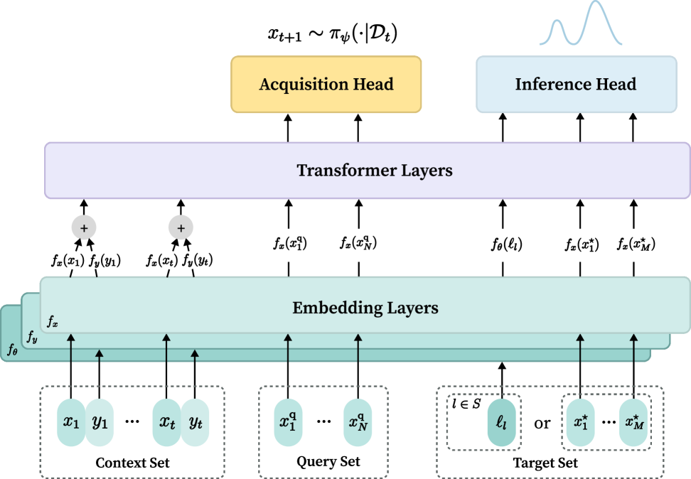
Figure A1: The Aline architecture. The model takes historical observations (Context Set), candidate query points (Query Set), and the current inference goal (Target Set) as inputs. These are transformed by Embedding Layers and subsequently by Transformer Layers. Finally, an Acquisition Head determines the next data point to query, while an Inference Head performs the approximate Bayesian inference.

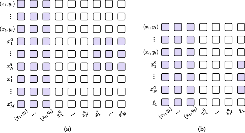
Figure A2: Example attention masks in Aline’s transformer architecture. (a) Mask for a predictive target $\xi=\xi_{p_{\star}}^{{y}^{\star}}$ (b) Mask for a parameter target $\xi=\xi_{\{1\}}^{\theta}$. Shaded squares indicate allowed attention.

Appendix C Experimental details

This section provides details for the experimental setups. Section˜C.1 outlines the specifics for the active learning experiments in Section˜5.1, including the synthetic function sampling procedures (Section˜C.1.1), implementation details for baseline methods (Section˜C.1.2), and training and evaluation details for these tasks (Section˜C.1.3). Next, in Section˜C.2 we describe the details of BED tasks, including the task descriptions (Section˜C.2.1), implementation of the baselines (Section˜C.2.2), and the training and evaluation details (Section˜C.2.3). Lastly, Section˜C.3 contains the specifics of the psychometric modeling experiments, detailing the psychometric function we use (Section˜C.3.1) and the setup for the experimental comparisons (Section˜C.3.2).

C.1 Active learning for regression and hyperparameter inference

C.1.1 Synthetic functions sampling procedure

For active learning tasks, Aline is trained exclusively on synthetically generated Gaussian Process (GP) functions. The procedure for generating these functions is as follows. First, the hyperparameters of the GP kernels, namely the output scale and lengthscale(s), are sampled from their respective prior distributions. For multi-dimensional input spaces ($d_{x}>1$), there is a $p_{\text{iso}}=0.5$ probability that an isotropic kernel is used, meaning that all input dimensions share a common lengthscale. Otherwise, an anisotropic kernel is employed, with a distinct lengthscale sampled for each input dimension. Subsequently, a kernel function is chosen randomly from a pre-defined set, with each kernel having a uniform probability of selection. In our experiments, we utilize the Radial Basis Function (RBF), Matérn 3/2, and Matérn 5/2 kernels.

The kernel’s output scale is sampled uniformly from the interval $U(0.1,1)$. The lengthscale(s) are sampled from $U(0.1,2)\times\sqrt{d_{x}}$. Input data points $x$ are sampled uniformly within the range $[-5,5]$ for each dimension. Finally, Gaussian noise with a fixed standard deviation of $0.01$ is added to the true function output $y$ for each sampled data point. Figure˜A3 illustrates some examples of the synthetic GP functions generated using this procedure.

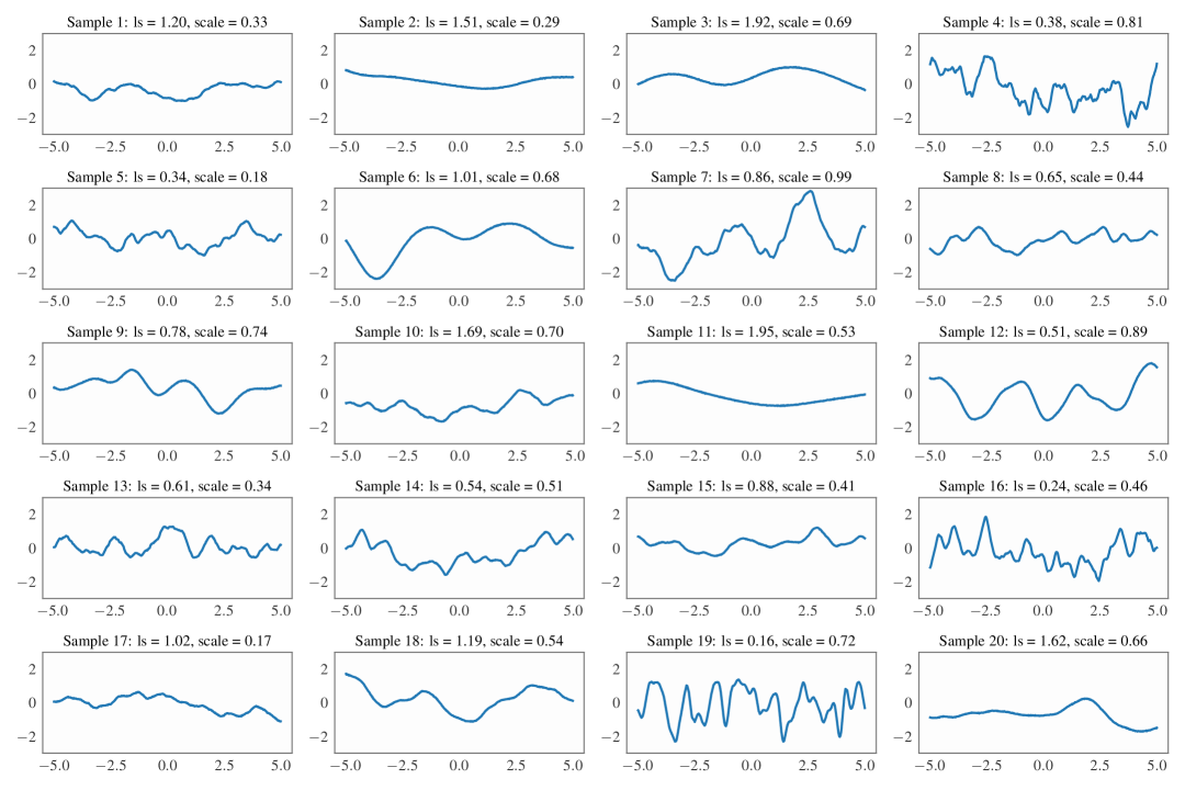
Figure A3: Examples of randomly sampled 1D synthetic GP functions used to train Aline.

C.1.2 Details of acquisition functions

We compare Aline with four commonly used AL acquisition functions. For Random Sampling (RS), we randomly select one point from the candidate pool as the next query point.

Uncertainty Sampling (US) is a simple and widely used AL acquisition strategy that prioritizes points where the model is most uncertain about its prediction:

$$\text{US}(x)=\sqrt{\mathbb{V}[y\,|\,x,\mathcal{D}]},$$ (A16)

where $\mathbb{V}[y\,|\,x,\mathcal{D}]$ is the predictive variance at $x$ given the current training data $\mathcal{D}$.

Variance Reduction (VR) (Yu et al.,, 2006) aims to select a candidate point that is expected to maximally reduce the predictive variance over a pre-defined test set $\{x^{\star}_{m}\}_{m=1}^{M}$, which is defined as:

$$\text{VR}(x)=\frac{\sum_{m=1}^{M}\left(\text{Cov}_{\text{post}}(x^{\star},x)\right)^{2}}{\mathbb{V}[y\,|\,x,\mathcal{D}]},$$ (A17)

$\text{Cov}_{\text{post}}(x^{\star},x)$ is the posterior covariance between the latent function values at $x^{\star}$ and $x$, given the history $\mathcal{D}=\{(X_{\text{train}},y_{\text{train}})\}$, where $X_{\text{train}}$ comprises all currently observed inputs with $y_{\text{train}}$ being their corresponding outputs. It is computed as:

$$\text{Cov}_{\text{post}}(x^{\star},x)=k(x^{\star},x)-k(x^{\star},X_{\text{train}})(K_{\text{train}}+\alpha I)^{-1}k(X_{\text{train}},x).$$ (A18)

Here, $k(\cdot,\cdot)$ is the GP kernel function, $K_{\text{train}}=k(X_{\text{train}},X_{\text{train}})$, and $\alpha$ is the noise variance.

Expected Predictive Information Gain (EPIG) (Smith et al.,, 2023) measures the expected reduction in predictive uncertainty on a target input distribution $p_{\star}(x^{\star})$. Following Smith et al., (2023), for a Gaussian predictive distribution, the EPIG for a candidate point can be expressed as:

$$\text{EPIG}(x)=\mathbb{E}_{p_{\star}(x^{\star})}[\frac{1}{2}\log\frac{\mathbb{V}[y\,|\,x,\mathcal{D}]\mathbb{V}[{y}^{\star}\,|\,x^{\star},\mathcal{D}]}{\mathbb{V}[y\,|\,x,\mathcal{D}]\mathbb{V}[{y}^{\star}\,|\,x^{\star},\mathcal{D}]-\text{Cov}_{\text{post}}(x^{\star},x)^{2}}].$$ (A19)

In practice, we approximate it by averaging over $m$ sampled test points:

$$\text{EPIG}(x)\approx\frac{1}{2M}\sum_{m=1}^{M}\log\frac{\mathbb{V}[y\,|\,x,\mathcal{D}]\mathbb{V}[{y}^{\star}_{m}\,|\,x^{\star}_{m},\mathcal{D}]}{\mathbb{V}[y\,|\,x,\mathcal{D}]\mathbb{V}[{y}^{\star}_{m}\,|\,x^{\star}_{m},\mathcal{D}]-\text{Cov}_{\text{post}}(x^{\star}_{m},x)^{2}}.$$ (A20)

C.1.3 Training and evaluation details

For both 1D and 2D input scenarios, Aline is trained for $2\cdot 10^{5}$ epochs using a batch size of 200. The discount factor $\gamma$ for the policy gradient loss is set to 1. For the GP-based baselines, we utilized Gaussian Process Regressors implemented via the scikit-learn library (Pedregosa et al.,, 2011). The hyperparameters of the GP models are optimized at each step. For the ACE baseline (Chang et al.,, 2025), we use a transformer architecture and an inference head design consistent with our Aline model.

All active learning experiments are evaluated with a candidate query pool consisting of 500 points. Each experimental run commenced with an initial context set consisting of a single data point. The target set size for predictive tasks is set to 100.

C.2 Benchmarking on Bayesian experimental design tasks

C.2.1 Task descriptions

Location Finding (Sheng and Hu,, 2004) is a benchmark problem commonly used in BED literature (Foster et al.,, 2019; Ivanova et al.,, 2021; Blau et al.,, 2022; Ivanova et al.,, 2024). The objective is to infer the unknown positions of $K$ hidden sources, $\theta=\{\theta_{k}\in\mathbb{R^{d}}\}_{k=1}^{K}$, by strategically selecting a sequence of observation locations, $x\in\mathbb{R}^{d}$. Each source emits a signal whose intensity attenuates with distance following an inverse-square law. The total signal intensity at an observation location $x$ is given by the superposition of signals from all sources:

$$\mu(\theta,x)=b+\sum_{k=1}^{K}\frac{\alpha_{k}}{m+\|\theta_{k}-x\|^{2}},$$ (A21)

where $\alpha_{k}$ are known source strength constants, and $b,m>0$ are constants controlling the background level and maximum signal intensity, respectively. In this experiment, we use $K=1$, $d=2$, $\alpha_{k}=1$, $b=0.1$ and $m=10^{-4}$, and the prior distribution over each component of a source’s location $\theta_{k}=(\theta_{k,1},...,\theta_{k,d})$ is uniform over the interval $[0,1]$.

The observation is modeled as the log-transformed total intensity corrupted by Gaussian noise:

$$\log y\,|\,\theta,x\sim\mathcal{N}(\log\mu(\theta,x),\sigma^{2}),$$ (A22)

where we use $\sigma=0.5$ in our experiments.

Constant Elasticity of Substitution (CES) (Arrow et al.,, 1961) considers a behavioral economics problem in which a participant compares two baskets of goods and rates the subjective difference in utility between the baskets on a sliding scale from 0 to 1. The utility of a basket $z$, consisting of $K$ goods with different values, is characterized by latent parameters $\theta=(\rho,\bm{\alpha},\mu)$. The design problem is to select pairs of baskets, $x=(z,z^{\prime})\in[0,100]^{2K}$, to infer the participant’s latent utility parameters.

The utility of a basket $z$ is defined using the constant elasticity of substitution function, as:

$$U(z)=\left(\sum_{i=1}^{K}z_{i}^{\rho}\alpha_{i}\right)^{\frac{1}{\rho}}.$$ (A23)

The prior of the latent parameters is specified as:

$$\begin{split}\rho&\sim\mathrm{Beta}(1,1)\\ \bm{\alpha}&\sim\mathrm{Dirichlet}(\mathbf{1}_{K})\\ \log u&\sim\mathcal{N}(1,3^{2}).\end{split}$$ (A24)

The subjective utility difference between two baskets is modeled as follows:

$$\begin{split}\eta&\sim\mathcal{N}\left(u\cdot\left(U(z)-U\left(z^{\prime}\right)\right),u^{2}\cdot\tau^{2}\cdot\left(1+\left\|z-z^{\prime}\right\|\right)^{2}\right)\\ y&=\mathrm{clip}(\mathrm{sigmoid}(\eta),\epsilon,1-\epsilon).\end{split}$$ (A25)

In this experiment, we choose $K=3$, $\tau=0.005$ and $\epsilon=2^{-22}$.

C.2.2 Implementation details of baselines

We compare Aline with four baseline methods. For Random Design policy, we randomly sample a design from the design space using a uniform distribution.

VPCE (Foster et al.,, 2020) iteratively infers the posterior through variational inference and maximizes the myopic Prior Contrastive Estimation (PCE) lower bound by gradient descent with respect to the experimental design. The hyperparameters used in the experiments are given in LABEL:tab:vpce_configurations.

Table A1: Additional hyperparameters used in VPCE (Foster et al.,, 2020).

Parameter	Location Finding	CES
VI gradient steps	1000	1000
VI learning rate	$10^{-3}$	$10^{-3}$
Design gradient steps	2500	2500
Design learning rate	$10^{-3}$	$10^{-3}$
Contrastive samples $L$	500	10
Expectation samples	500	10

Deep Adaptive Design (DAD) (Foster et al.,, 2021) learns an amortized design policy guided by sPCE lower bound. For a design policy $\pi$, and $L\geq 0$ contrastive samples, sPCE over a sequence of $T$ experiments is defined as:

$$\mathcal{L}_{T}(\pi,L)=\mathbb{E}_{p\left(\theta_{0},\mathcal{D}_{T}\mid\pi\right)p\left(\theta_{1:L}\right)}\left[\log\frac{p\left(\mathcal{D}_{T}\mid\theta_{0},\pi\right)}{\frac{1}{L+1}\sum_{\ell=0}^{L}p\left(\mathcal{D}_{T}\mid\theta_{\ell},\pi\right)}\right],$$ (A26)

where the contrastive samples $\theta_{1:L}$ are drawn independently from the prior $p(\theta)$. The bound becomes tight as $L\rightarrow\infty$, with a convergence rate of $\mathcal{O}(L^{-1})$.

The design network comprises an MLP encoder that encodes historical data into a fixed-dimensional representation, and an MLP emitter that proposes the next design point. The encoder processes the concatenated design-observation pairs from history and aggregates their representations through a pooling operation.

Following the work of Foster et al., (2021), the encoder network consists of two fully connected layers with 128 and 16 units with ReLU activation applied to the hidden layer. The emitter is implemented as a fully connected layer that maps the pooled representation to the design space. The policy is trained using the Adam optimizer with an initial learning rate of $5\cdot 10^{-5}$, $\beta=(0.8,0.998)$, and an exponentially decaying learning rate, reduced by a factor of $\gamma=0.98$ every 1000 epochs. In the Location Finding task, the model is trained for $10^{5}$ epochs, and $10^{4}$ contrastive samples are utilized in each training step for the estimation of the sPCE lower bound. Note that, for the CES task, we applied several adjustments, including normalizing the input, applying the Sigmoid and Softplus transformations to the output before mapping it to the design space, increasing the depth of the network, and initializing weights using Xavier initialization (Glorot and Bengio,, 2010). However, DAD failed to converge during training in our experiments. Therefore, we report the results provided by Blau et al., (2022).

RL-BOED (Blau et al.,, 2022) frames the design policy optimization as a Markov Decision Process (MDP) and employs reinforcement learning to learn the design policy. It utilizes a stepwise reward function to estimate the marginal contribution of the $t$-th experiment to the sEIG.

The design network shares a similar backbone architecture to that of DAD, with the exception that the deterministic output of the emitter is replaced by a Tanh-Gaussian distribution. The encoder comprises two fully connected layers with 128 units and ReLU activation, followed by an output layer with 64 units and no activation. Training is conducted using Randomized Ensembled Double Q-learning (REDQ) (Chen et al.,, 2021), the full configurations are reported in LABEL:tab:rl_boed_configurations.

Table A2: Additional hyperparameters used in RL-BOED (Blau et al.,, 2022).

Parameter	Location Finding	CES
Critics	2	2
Random subsets	2	2
Contrastive samples $L$	$10^{5}$	$10^{5}$
Training epochs	$10^{5}$	$5\cdot 10^{4}$
Discount factor $\gamma$	0.9	0.9
Target update rate	$10^{-3}$	$5\cdot 10^{-3}$
Policy learning rate	$10^{-4}$	$3\cdot 10^{-4}$
Critic learning rate	$3\cdot 10^{-4}$	$3\cdot 10^{-4}$
Buffer size	$10^{7}$	$10^{6}$

C.2.3 Training and evaluation details

In the Location Finding task, the number of sequential design steps, $T$, is set to 30. For all evaluated methods, the sPCE lower bound is estimated using $L=10^{6}$ contrastive samples. The Aline is trained over $10^{5}$ epochs with a batch size of 200. The discount factor $\gamma$ for the policy gradient loss is set to 1. During the evaluation phase, the query set consists of 2000 points, which are drawn uniformly from the defined design space. For the CES task, each experimental run consists of $T=10$ design steps. The sPCE lower bound is estimated using $L=10^{7}$ contrastive samples. The Aline is trained for $2\cdot 10^{5}$ epochs with a batch size of 200, and we use 2000 for the query set size.

C.3 Psychometric model

C.3.1 Model description

In this experiment, we use a four-parameter psychometric function with the following parameterization:

$$\pi(x)=\theta_{3}\cdot\theta_{4}+(1-\theta_{4})F(\frac{x-\theta_{1}}{\theta_{2}}),$$

where:

• $\theta_{1}$ (threshold): The stimulus intensity at which the probability of a positive response reaches a specific criterion. It represents the location of the psychometric curve. We use a uniform prior $U[-3,3]$ for $\theta_{1}$.

• $\theta_{2}$ (slope): Describes the steepness of the psychometric function. Smaller values of $\theta_{2}$ indicate a sharper transition, reflecting higher sensitivity around the threshold. We use a uniform prior $U[0.1,2]$ for $\theta_{2}$.

• $\theta_{3}$ (guess rate): The baseline response probability for stimuli far below the threshold, reflecting responses made by guessing. We use a uniform prior $U[0.1,0.9]$ for $\theta_{3}$.

• $\theta_{4}$ (lapse rate): The rate at which the observer makes errors independent of stimulus intensity, representing an upper asymptote on performance below 1. We use a uniform prior $U[0,0.5]$ for $\theta_{4}$.

We employ a Gumbel-type internal link function $F=1-e^{-10^{z}}$ where $z=\frac{x-\theta_{1}}{\theta_{2}}$. Lastly, a binary response $y$ is simulated from the psychometric function $\pi(x)$ using a Bernoulli distribution with probability of success $p=\pi(x)$.

C.3.2 Experimental details

We compare Aline against two established Bayesian adaptive methods:

• QUEST+ (Watson,, 2017): QUEST+ is an adaptive psychometric procedure that aims to find the stimulus that maximizes the expected information gain about the parameters of the psychometric function, or equivalently, minimizes the expected entropy of the posterior distribution over the parameters. It typically operates on a discrete grid of possible parameter values and selects stimuli to reduce uncertainty over this entire joint parameter space. In our experiments, QUEST+ is configured to infer all four parameters simultaneously.

• Psi-marginal (Prins,, 2013): The Psi-marginal method is an extension of the psi method (Kontsevich and Tyler,, 1999) that allows for efficient inference by marginalizing over nuisance parameters. When specific parameters are designated as targets of interest, Psi-marginal optimizes stimulus selection to maximize information gain specifically for these target parameters, effectively treating the others as nuisance variables. This makes it highly efficient when only a subset of parameters is critical.

For each simulated experiment, true underlying parameters are sampled from their prior distributions. Stimulus values $x$ are selected from a discrete set of size 200 drawn uniformly from the range $[-5,5]$.

Appendix D Additional experimental results

D.1 Active learning for regression and hyperparameter inference

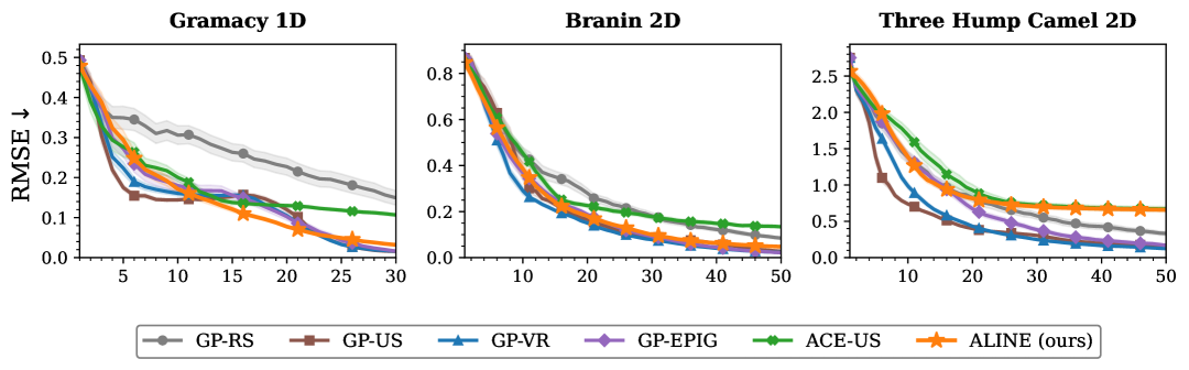
Figure A4: Predictive performance in terms of RMSE on three other active learning benchmark functions. Results show the mean and 95% confidence interval (CI) across 100 runs. Notably, on the Three Hump Camel function, the performance of amortized methods like Aline and ACE-US is limited, as its output scale significantly differs from the pre-training distribution, highlighting a scenario of distribution shift.

AL results on more benchmark functions.

To further assess Aline, we present performance evaluations on an additional set of active learning benchmark functions, see Figure˜A4. The results on Gramacy and Branin show that we are on par with the GP baselines. For Three Hump Camel, we see both Aline and ACE-US showing reduced accuracy. This is because the function’s output value range extends beyond that of the GP functions used during pre-training. This highlights a potential area for future work, such as training Aline on a broader prior distribution of functions, potentially leading to more universally capable models.

Acquisition visualization for AL.

To qualitatively understand the behavior of our model, we visualize the query strategy employed by Aline for AL on a randomly sampled synthetic function Figure˜A5. This visualization illustrates how Aline iteratively selects query points to reduce uncertainty and refine its predictive posterior.

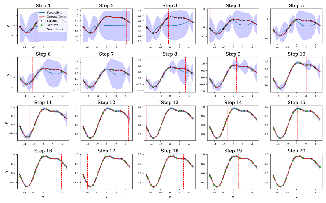
Figure A5: Sequential query strategy of Aline on a 1D synthetic GP function over 20 steps. As more points are queried, the model’s prediction increasingly aligns with the ground truth, and the uncertainty is strategically reduced.

Hyperparameter inference visualization.

We now visualize the evolution of Aline’s estimated posterior distributions for the underlying GP hyperparameters for a randomly drawn 2D synthetic GP function (see Figure˜A6). The posteriors are shown after 1, 15, and 30 active data acquisition steps. As Aline strategically queries more informative data points, its posterior beliefs about these generative parameters become increasingly concentrated and accurate.

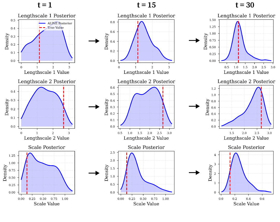
Figure A6: Estimated posteriors for the two lengthscales and the output scale obtained from Aline after $t=1$, $t=15$, and $t=30$ active query steps. The posteriors progressively concentrate around the true parameter values as more data is acquired.

Inference time.

To assess the computational efficiency of Aline, we report the inference times for the AL tasks in Table˜A3. The times represent the total duration to complete a sequence of 30 steps for 1D functions and 50 steps for 2D functions, averaged over 10 independent runs. As both Aline and ACE-US perform inference via a single forward pass per step once trained, they are significantly faster compared to traditional GP-based methods.

Table A3: Comparison of inference times (seconds) for different AL methods on 1D (30 steps) and 2D (50 steps) tasks. Values are averaged over 10 runs (mean $\pm$ standard deviation).

Methods	Inference time (s)
	1D & 30 steps	2D & 50 steps
GP-US	0.62$\pm$0.09	1.72$\pm$0.23
GP-VR	1.41$\pm$0.14	4.03$\pm$0.18
GP-EPIG	1.34$\pm$0.11	3.43$\pm$0.24
ACE-US	0.08$\pm$0.00	0.19$\pm$0.02
Aline	0.08$\pm$0.00	0.19$\pm$0.02

D.2 Benchmarking on Bayesian experimental design tasks

In this section, we provide additional qualitative results for Aline’s performance on the BED benchmark tasks. Specifically, for the Location Finding task, we visualize the sequence of designs chosen by Aline and the resulting posterior distribution over the hidden source’s location (Figure˜A7). For the CES task, we present the estimated marginal posterior distributions for the model parameters, comparing them against their true underlying values (Figure˜A8). We see that Aline offers accurate parameter inference.

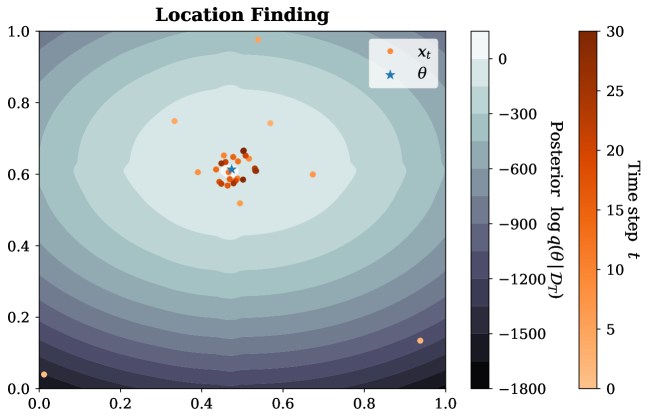
Figure A7: Visualization of Aline’s design policy and resulting posterior for the Location Finding task. The contour plot shows the log posterior probability density of the source location $\theta$ (true location marked by blue star) after $T=30$ steps. Queried locations, with color indicating the time step of acquisition, demonstrating a concentration of queries around the true source.

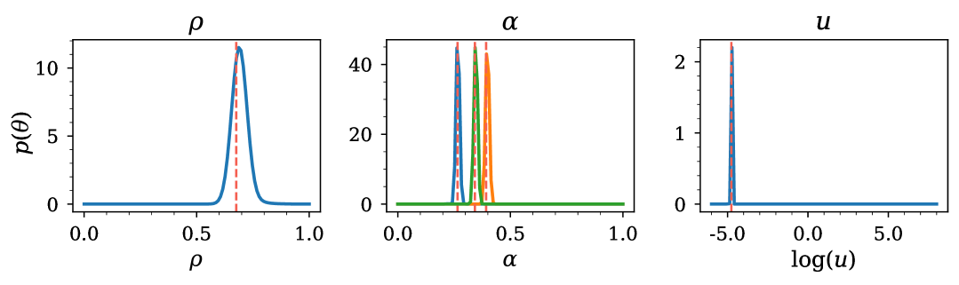
Figure A8: Aline’s estimated marginal posterior distributions for the parameters of the CES task after $T=10$ query steps. The dashed red lines indicate the true parameter values. The posteriors are well-concentrated around the true values, demonstrating accurate parameter inference.

D.3 Psychometric model

Targeted vs. full parameter acquisition.

To further demonstrate the advantage of Aline’s flexible targeting capability, we conduct an additional experiment within the psychometric modeling task. We evaluate two configurations: one where Aline specifically targets a subset of parameters (targeted), which we show in the main text, and another configuration where Aline aims to infer all four parameters simultaneously (full). As illustrated in Figure˜A9, directing Aline’s data acquisition strategy towards a specific parameter subset results in more accurate posterior inference for those targeted parameters compared to when Aline is tasked with learning all parameters concurrently. This underscores the benefit of targeted querying for achieving enhanced precision on parameters of primary interest.

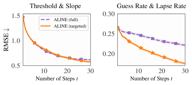
Figure A9: Performance comparison for two Aline configurations under psychometric model. Aline (full) targets all four psychometric parameters simultaneously, and Aline (targeted) focuses on specific parameter subsets. When specifically targeting the guess and lapse rates, Aline (targeted) achieves significantly lower error for this subset compared to the Aline (full) version, demonstrating the benefit of its flexible focusing capability for improved parameter inference.

Inference time.

We additionally assess the computational efficiency of each method in proposing the next design point. The average per-step design proposal time, measured over the 30-step psychometric experiments across 20 runs, is $0.002\pm 0.00$s for Aline, $0.07\pm 0.00$s for QUEST+, and $0.02\pm 0.00$s for Psi-marginal. Methods like QUEST+ and Psi-marginal, which often rely on grid-based posterior estimation, face rapidly increasing computational costs as the parameter space dimensionality or required grid resolution grows. Aline, however, estimates the posterior via the transformer in a single forward pass, making its inference time largely insensitive to these factors. Thus, this computational efficiency gap is anticipated to become even more pronounced for more complex psychometric models.

Appendix E Computational resources and software

All experiments presented in this work, encompassing model development, hyperparameter optimization, baseline evaluations, and preliminary analyses, are performed on a GPU cluster equipped with AMD MI250X GPUs. The total computational resources consumed for this research, including all development stages and experimental runs, are estimated to be approximately 5000 GPU hours. For each experiment, it takes around 20 hours to train an Aline model for $10^{5}$ epochs. The core code base is built using Pytorch (https://pytorch.org/, License: modified BSD license). For the Gaussian Process (GP) based baselines, we utilize Scikit-learn (Pedregosa et al.,, 2011) (https://scikit-learn.org/, License: modified BSD license). The DAD baseline is adapted from the original authors’ publicly available code (Foster et al.,, 2021) (https://github.com/ae-foster/dad; MIT License). Our implementation of the RL-BOED baseline uses the repository provided by (Barlas and Salako,, 2025) (https://github.com/yasirbarlas/RL-BOED; MIT License). We use questplus package (https://github.com/hoechenberger/questplus, License: GPL-3.0) to implement QUEST+, and use Psi-staircase (https://github.com/NNiehof/Psi-staircase, License: GPL-3.0) to implement the Psi-marginal method.

References

- Arrow et al., (1961) Arrow, K. J., Chenery, H. B., Minhas, B. S., and Solow, R. M. (1961). Capital-labor substitution and economic efficiency. The Review of Economics and Statistics, 43(3):225–250.
- (2) Ashman, M., Diaconu, C., Kim, J., Sivaraya, L., Markou, S., Requeima, J., Bruinsma, W. P., and Turner, R. E. (2024a). Translation equivariant transformer neural processes. In International Conference on Machine Learning, pages 1924–1944. PMLR.
- (3) Ashman, M., Diaconu, C., Weller, A., and Turner, R. E. (2024b). In-context in-context learning with transformer neural processes. In Symposium on Advances in Approximate Bayesian Inference, pages 1–29. PMLR.
- Barlas and Salako, (2025) Barlas, Y. Z. and Salako, K. (2025). Performance comparisons of reinforcement learning algorithms for sequential experimental design. arXiv preprint arXiv:2503.05905.
- Berry et al., (2010) Berry, S. M., Carlin, B. P., Lee, J. J., and Muller, P. (2010). Bayesian adaptive methods for clinical trials. CRC press.
- Blau et al., (2023) Blau, T., Bonilla, E., Chades, I., and Dezfouli, A. (2023). Cross-entropy estimators for sequential experiment design with reinforcement learning. arXiv preprint arXiv:2305.18435.
- Blau et al., (2022) Blau, T., Bonilla, E. V., Chades, I., and Dezfouli, A. (2022). Optimizing sequential experimental design with deep reinforcement learning. In International conference on machine learning, pages 2107–2128. PMLR.
- Broderick et al., (2013) Broderick, T., Boyd, N., Wibisono, A., Wilson, A. C., and Jordan, M. I. (2013). Streaming variational bayes. Advances in neural information processing systems, 26.
- Bruinsma et al., (2023) Bruinsma, W., Markou, S., Requeima, J., Foong, A. Y., Andersson, T., Vaughan, A., Buonomo, A., Hosking, S., and Turner, R. E. (2023). Autoregressive conditional neural processes. In The Eleventh International Conference on Learning Representations.
- Bruinsma et al., (2020) Bruinsma, W., Requeima, J., Foong, A. Y., Gordon, J., and Turner, R. E. (2020). The gaussian neural process. In Third Symposium on Advances in Approximate Bayesian Inference.
- Carpenter et al., (2017) Carpenter, B., Gelman, A., Hoffman, M. D., Lee, D., Goodrich, B., Betancourt, M., Brubaker, M., Guo, J., Li, P., and Riddell, A. (2017). Stan: A probabilistic programming language. Journal of statistical software, 76:1–32.
- Chaloner and Verdinelli, (1995) Chaloner, K. and Verdinelli, I. (1995). Bayesian experimental design: A review. Statistical science, pages 273–304.
- Chang et al., (2025) Chang, P. E., Loka, N., Huang, D., Remes, U., Kaski, S., and Acerbi, L. (2025). Amortized probabilistic conditioning for optimization, simulation and inference. In International Conference on Artificial Intelligence and Statistics. PMLR.
- Chen et al., (2021) Chen, X., Wang, C., Zhou, Z., and Ross, K. W. (2021). Randomized ensembled double q-learning: Learning fast without a model. In International Conference on Learning Representations.
- Cranmer et al., (2020) Cranmer, K., Brehmer, J., and Louppe, G. (2020). The frontier of simulation-based inference. Proceedings of the National Academy of Sciences, 117(48):30055–30062.
- Doucet et al., (2001) Doucet, A., De Freitas, N., Gordon, N. J., et al. (2001). Sequential Monte Carlo methods in practice, volume 1. Springer.
- Feng et al., (2023) Feng, L., Hajimirsadeghi, H., Bengio, Y., and Ahmed, M. O. (2023). Latent bottlenecked attentive neural processes. In The Eleventh International Conference on Learning Representations.
- Feng et al., (2024) Feng, L., Tung, F., Hajimirsadeghi, H., Bengio, Y., and Ahmed, M. O. (2024). Memory efficient neural processes via constant memory attention block. In International Conference on Machine Learning, pages 13365–13386. PMLR.
- Filstroff et al., (2024) Filstroff, L., Sundin, I., Mikkola, P., Tiulpin, A., Kylmäoja, J., and Kaski, S. (2024). Targeted active learning for bayesian decision-making. Transactions on Machine Learning Research.
- Forster et al., (2025) Forster, A., Ivanova, D. R., and Rainforth, T. (2025). Improving robustness to model misspecification in bayesian experimental design. In 7th Symposium on Advances in Approximate Bayesian Inference Workshop Track.
- Foster et al., (2021) Foster, A., Ivanova, D. R., Malik, I., and Rainforth, T. (2021). Deep adaptive design: Amortizing sequential bayesian experimental design. In International Conference on Machine Learning, pages 3384–3395. PMLR.
- Foster et al., (2019) Foster, A., Jankowiak, M., Bingham, E., Horsfall, P., Teh, Y. W., Rainforth, T., and Goodman, N. (2019). Variational bayesian optimal experimental design. Advances in Neural Information Processing Systems, 32.
- Foster et al., (2020) Foster, A., Jankowiak, M., O’Meara, M., Teh, Y. W., and Rainforth, T. (2020). A unified stochastic gradient approach to designing bayesian-optimal experiments. In International Conference on Artificial Intelligence and Statistics, pages 2959–2969. PMLR.
- (24) Garnelo, M., Rosenbaum, D., Maddison, C., Ramalho, T., Saxton, D., Shanahan, M., Teh, Y. W., Rezende, D., and Eslami, S. A. (2018a). Conditional neural processes. In International conference on machine learning, pages 1704–1713. PMLR.
- (25) Garnelo, M., Schwarz, J., Rosenbaum, D., Viola, F., Rezende, D. J., Eslami, S., and Teh, Y. W. (2018b). Neural processes. arXiv preprint arXiv:1807.01622.
- Gelman et al., (2013) Gelman, A., Carlin, J. B., Stern, H. S., Dunson, D. B., Vehtari, A., and Rubin, D. B. (2013). Bayesian Data Analysis. CRC Press.
- Gilaie-Dotan et al., (2013) Gilaie-Dotan, S., Kanai, R., Bahrami, B., Rees, G., and Saygin, A. P. (2013). Neuroanatomical correlates of biological motion detection. Neuropsychologia, 51(3):457–463.
- Giovagnoli, (2021) Giovagnoli, A. (2021). The bayesian design of adaptive clinical trials. International journal of environmental research and public health, 18(2):530.
- Gloeckler et al., (2024) Gloeckler, M., Deistler, M., Weilbach, C. D., Wood, F., and Macke, J. H. (2024). All-in-one simulation-based inference. In International Conference on Machine Learning, pages 15735–15766. PMLR.
- Glorot and Bengio, (2010) Glorot, X. and Bengio, Y. (2010). Understanding the difficulty of training deep feedforward neural networks. In Teh, Y. W. and Titterington, M., editors, Proceedings of the Thirteenth International Conference on Artificial Intelligence and Statistics, volume 9 of Proceedings of Machine Learning Research, pages 249–256, Chia Laguna Resort, Sardinia, Italy. PMLR.
- Gordon et al., (2020) Gordon, J., Bruinsma, W. P., Foong, A. Y., Requeima, J., Dubois, Y., and Turner, R. E. (2020). Convolutional conditional neural processes. In International Conference on Learning Representations.
- Greenberg et al., (2019) Greenberg, D., Nonnenmacher, M., and Macke, J. (2019). Automatic posterior transformation for likelihood-free inference. In International conference on machine learning, pages 2404–2414. PMLR.
- (33) Huang, D., Bharti, A., Souza, A., Acerbi, L., and Kaski, S. (2023a). Learning robust statistics for simulation-based inference under model misspecification. Advances in Neural Information Processing Systems, 36:7289–7310.
- Huang et al., (2025) Huang, D., Guo, Y., Acerbi, L., and Kaski, S. (2025). Amortized bayesian experimental design for decision-making. Advances in Neural Information Processing Systems, 37:109460–109486.
- (35) Huang, D., Haussmann, M., Remes, U., John, S., Clarté, G., Luck, K., Kaski, S., and Acerbi, L. (2023b). Practical equivariances via relational conditional neural processes. Advances in Neural Information Processing Systems, 36:29201–29238.
- Hung et al., (2025) Hung, Y. H., Lin, K.-J., Lin, Y.-H., Wang, C.-Y., Sun, C., and Hsieh, P.-C. (2025). Boformer: Learning to solve multi-objective bayesian optimization via non-markovian rl. In The Thirteenth International Conference on Learning Representations.
- Ivanova et al., (2021) Ivanova, D. R., Foster, A., Kleinegesse, S., Gutmann, M. U., and Rainforth, T. (2021). Implicit deep adaptive design: Policy-based experimental design without likelihoods. Advances in Neural Information Processing Systems, 34.
- Ivanova et al., (2024) Ivanova, D. R., Hedman, M., Guan, C., and Rainforth, T. (2024). Step-DAD: Semi-Amortized Policy-Based Bayesian Experimental Design. ICLR 2024 Workshop on Data-centric Machine Learning Research (DMLR).
- Kim et al., (2019) Kim, H., Mnih, A., Schwarz, J., Garnelo, M., Eslami, A., Rosenbaum, D., Vinyals, O., and Teh, Y. W. (2019). Attentive neural processes. In International Conference on Learning Representations.
- Kontsevich and Tyler, (1999) Kontsevich, L. L. and Tyler, C. W. (1999). Bayesian adaptive estimation of psychometric slope and threshold. Vision research, 39(16):2729–2737.
- Krause et al., (2006) Krause, A., Guestrin, C., Gupta, A., and Kleinberg, J. (2006). Near-optimal sensor placements: Maximizing information while minimizing communication cost. In Proceedings of the 5th international conference on Information processing in sensor networks, pages 2–10.
- Lee et al., (2025) Lee, H., Jang, C., Lee, D. B., and Lee, J. (2025). Dimension agnostic neural processes. In The Thirteenth International Conference on Learning Representations.
- Li et al., (2025) Li, C.-Y., Toussaint, M., Rakitsch, B., and Zimmer, C. (2025). Amortized safe active learning for real-time decision-making: Pretrained neural policies from simulated nonparametric functions. arXiv preprint arXiv:2501.15458.
- Lindley, (1956) Lindley, D. V. (1956). On a measure of the information provided by an experiment. The Annals of Mathematical Statistics, 27(4):986–1005.
- Lookman et al., (2019) Lookman, T., Balachandran, P. V., Xue, D., and Yuan, R. (2019). Active learning in materials science with emphasis on adaptive sampling using uncertainties for targeted design. npj Computational Materials, 5(1):21.
- Lueckmann et al., (2017) Lueckmann, J.-M., Goncalves, P. J., Bassetto, G., Öcal, K., Nonnenmacher, M., and Macke, J. H. (2017). Flexible statistical inference for mechanistic models of neural dynamics. Advances in neural information processing systems, 30.
- Maraval et al., (2024) Maraval, A., Zimmer, M., Grosnit, A., and Bou Ammar, H. (2024). End-to-end meta-bayesian optimisation with transformer neural processes. Advances in Neural Information Processing Systems, 36.
- Mittal et al., (2025) Mittal, S., Bracher, N. L., Lajoie, G., Jaini, P., and Brubaker, M. (2025). Amortized in-context bayesian posterior estimation. arXiv preprint arXiv:2502.06601.
- Müller et al., (2022) Müller, S., Hollmann, N., Arango, S. P., Grabocka, J., and Hutter, F. (2022). Transformers can do bayesian inference. In International Conference on Learning Representations.
- Nguyen and Grover, (2022) Nguyen, T. and Grover, A. (2022). Transformer neural processes: Uncertainty-aware meta learning via sequence modeling. In International Conference on Machine Learning, pages 16569–16594. PMLR.
- Papamakarios and Murray, (2016) Papamakarios, G. and Murray, I. (2016). Fast -free inference of simulation models with bayesian conditional density estimation. Advances in neural information processing systems, 29.
- Pasek and Krosnick, (2010) Pasek, J. and Krosnick, J. A. (2010). Optimizing survey questionnaire design in political science: Insights from psychology.
- Pedregosa et al., (2011) Pedregosa, F., Varoquaux, G., Gramfort, A., Michel, V., Thirion, B., Grisel, O., Blondel, M., Prettenhofer, P., Weiss, R., Dubourg, V., et al. (2011). Scikit-learn: Machine learning in python. the Journal of machine Learning research, 12:2825–2830.
- Powers et al., (2017) Powers, A. R., Mathys, C., and Corlett, P. R. (2017). Pavlovian conditioning–induced hallucinations result from overweighting of perceptual priors. Science, 357(6351):596–600.
- Prins, (2013) Prins, N. (2013). The psi-marginal adaptive method: How to give nuisance parameters the attention they deserve (no more, no less). Journal of vision, 13(7):3–3.
- (56) Radev, S. T., Schmitt, M., Pratz, V., Picchini, U., Köthe, U., and Bürkner, P.-C. (2023a). Jana: Jointly amortized neural approximation of complex bayesian models. In Uncertainty in Artificial Intelligence, pages 1695–1706. PMLR.
- (57) Radev, S. T., Schmitt, M., Schumacher, L., Elsemüller, L., Pratz, V., Schälte, Y., Köthe, U., and Bürkner, P.-C. (2023b). Bayesflow: Amortized bayesian workflows with neural networks. Journal of Open Source Software, 8(89):5702.
- Rainforth et al., (2024) Rainforth, T., Foster, A., Ivanova, D. R., and Bickford Smith, F. (2024). Modern bayesian experimental design. Statistical Science, 39(1):100–114.
- Rasmussen and Williams, (2006) Rasmussen, C. E. and Williams, C. K. (2006). Gaussian Processes for Machine Learning. MIT Press.
- Ryan et al., (2016) Ryan, E. G., Drovandi, C. C., McGree, J. M., and Pettitt, A. N. (2016). A review of modern computational algorithms for bayesian optimal design. International Statistical Review, 84(1):128–154.
- Schulman et al., (2015) Schulman, J., Levine, S., Abbeel, P., Jordan, M., and Moritz, P. (2015). Trust region policy optimization. In International conference on machine learning, pages 1889–1897. PMLR.
- Sheng and Hu, (2004) Sheng, X. and Hu, Y.-H. (2004). Maximum likelihood multiple-source localization using acoustic energy measurements with wireless sensor networks. IEEE transactions on signal processing, 53(1):44–53.
- Smith et al., (2023) Smith, F. B., Kirsch, A., Farquhar, S., Gal, Y., Foster, A., and Rainforth, T. (2023). Prediction-oriented bayesian active learning. In International Conference on Artificial Intelligence and Statistics, pages 7331–7348. PMLR.
- Sutton et al., (1999) Sutton, R. S., McAllester, D., Singh, S., and Mansour, Y. (1999). Policy gradient methods for reinforcement learning with function approximation. Advances in neural information processing systems, 12.
- Vaswani et al., (2017) Vaswani, A., Shazeer, N., Parmar, N., Uszkoreit, J., Jones, L., Gomez, A. N., Kaiser, Ł., and Polosukhin, I. (2017). Attention is all you need. Advances in neural information processing systems, 30.
- Watson, (2017) Watson, A. B. (2017). Quest+: A general multidimensional bayesian adaptive psychometric method. Journal of Vision, 17(3):10–10.
- Whittle et al., (2025) Whittle, G., Ziomek, J., Rawling, J., and Osborne, M. A. (2025). Distribution transformers: Fast approximate bayesian inference with on-the-fly prior adaptation. arXiv preprint arXiv:2502.02463.
- Wichmann and Hill, (2001) Wichmann, F. A. and Hill, N. J. (2001). The psychometric function: I. Fitting, sampling, and goodness of fit. Perception & Psychophysics, 63(8):1293–1313.
- Xu et al., (2024) Xu, C., Hülsmeier, D., Buhl, M., and Kollmeier, B. (2024). How does inattention influence the robustness and efficiency of adaptive procedures in the context of psychoacoustic assessments via smartphone? Trends in Hearing, 28:23312165241288051.
- Yu et al., (2006) Yu, K., Bi, J., and Tresp, V. (2006). Active learning via transductive experimental design. In Proceedings of the 23rd international conference on Machine learning, pages 1081–1088.
- Zammit-Mangion et al., (2024) Zammit-Mangion, A., Sainsbury-Dale, M., and Huser, R. (2024). Neural methods for amortised parameter inference. arXiv e-prints, pages arXiv–2404.
- Zhang et al., (2025) Zhang, X., Huang, D., Kaski, S., and Martinelli, J. (2025). Pabbo: Preferential amortized black-box optimization. In The Thirteenth International Conference on Learning Representations.