Revisiting Bäcklund-Darboux transformations for KP and BKP integrable hierarchies
ITEP-TH-19/25
We consider Bäcklund-Darboux transformations for integrable hierarchies of nonlinear equations such as KP, BKP and their close relatives referred to as modified KP and Schwarzian KP. We work in the framework of the bilinear formalism based on the bilinear equations for the tau-function. This approach allows one to extend the theory to fully difference (or discrete) versions of the integrable equations and their hierarchies in a natural way. We also show how to construct the Bäcklund-Darboux transformations in the operator approach developed by the Kyoto school, in which the tau-functions are represented as vacuum expectation values of certain operators made of free fermionic fields (charged for KP and neutral for BKP).
1 Introduction
Bäcklund-Darboux (BD) transformations acting in the space of exact solutions to integrable nonlinear partial differential or difference equations is an old and well studied subject. Generally speaking, such a transformation sends any solution of one or another integrable equation to another solution of the same or maybe a different equation. As soon as integrable equations are known to form infinite hierarchies of compatible equations, one may extend the notion of a BD transformation to the whole hierarchy. General solutions to such hierarchies as Kadomtsev-Petviashvili (KP), its B-version (BKP), 2D Toda lattice and other are provided by tau-functions , which are special functions of infinitely many independent variables (“times”) parametrizing commuting flows of the hierarchies. All other objects related to the integrable equations and their hierarchies such as Baker-Akhiezer functions, potentials and other types of dependent variables can be expressed through the tau-function by acting to it by certain differential or difference operators. In this paper, we consider the BD transformations of common solutions to the whole hierarchies: KP, modified KP (mKP), BKP as well as their difference/discrete analogs; and it is natural to do this on the level of tau-functions.
The existing literature on the subject is enormous, and there is no chance to cite the most part of it here. The standard sources are books [2, 3], which illuminate the subject from different points of view, and where many related references can be found. Among research papers, we mention here [4]–[9] and also [10, 11, 12, 13] for the reason that they had a great impact on the contents of the present paper.
This paper is an attempt to systematize the existing knowledge on the subject on the basis of the bilinear approach to the integrable hierarchies developed by Hirota and researches of the Kyoto school (see [14], [15, 16, 17] and also the book [18]), where the main hero is the tau-function , with being an infinite set of independent variables (“times”) which parametrize different commuting flows. The tau-function can be regarded as a universal dependent variable of the hierarchies. To much extent, the present paper should be regarded as a review; however, we do not exclude that some formulas and results, or their interpretation given here, were never mentioned in the literature in this form, so some of them are probably new.
The main motivation to write this paper was the need to achieve a better and a more detailed understanding of some elements of the theory which are related to BD transformations; such a requirement arose after writing the paper [19], where the BD transformations related to the classical mKP hierarchy appeared naturally in applications to spectral problems for integrable quantum spin chains. These quantum models are usually solved by means of one or another version of the celebrated Bethe ansatz, see, e.g. [20, 21, 22, 23]. The above mentioned applications of the BD transformations go back to papers [24]–[34], where it was realized that the nested Bethe ansatz method has a purely classical reincarnation as a chain of iterated BD transformations of trigonometric or rational solutions to the modified KP (for generalized spin chains with rational or trigonometric quantum -matrices) or KP (for models of the Gaudin type) hierarchy that allow one to “undress” the initial problem to a trivial one, hence obtaining a solution of the former. The nested Bethe equations themselves appear in this approach as equations of motion for poles of trigonometric or rational solutions to the hierarchies in discrete time. Eigenvalues of a special generating function of commuting operators (integrals of motion) in the quantum model appear as tau-functions of the classical hierarchies, with different eigenvalues in the spectrum corresponding to different solutions. We hope that the approach developed in this paper might help to clarify some yet uncovered secrets of Bethe ansatz, including a hypothetical extension of the approach initiated in [29] to quantum models with elliptic -matrices, which remains problematic so far.
The theory of BD transformations is closely related to the problem of integrable discretization of nonlinear partial differential equations such as KP, modified KP (mKP), BKP. A powerful general method for such discretization was suggested in [35] on the level of tau-functions. The key ingredient of this method is Miwa’s change of variables from the continuous times to a set of discrete variables first suggested in [36]:
| (1.1) |
where are parameters playng the role of inverse lattice spacings for the lattice variables .
Remarkably, the discrete variable that numbers different steps of a chain of iterated BD transformations enters the equations connecting neighboring members of the chain in the same way as the discrete variables that are introduced via Miwa’s substitution (1.1). Moreover, if we consider two or more such chains (each having its own discrete variable), then it is possible to write bilinear equations for the tau-function as function of these variables (and other variables of the hierarchy under consideration), and, again, the discrete variables corresponding to the chains enter the equations in a very similar way as those coming from the Miwa’s substitution. In particular, the equations obtained in this way that contain only shifts of the discrete variables numbering levels of the BD chains have precisely the same form as equations of the multi-component KP hierarchy introduced in [37] and further studied in [38]–[41].
As it was discovered by the Kyoto school [15, 16], the integrable hierarchies have a natural realization as quantum field theories of chiral 2D free fermions. In this approach, the tau-functions enter the game as vacuum expectation values of certain operators built from the Fermi-operators. The BD transformations have their natural interpretation in this language, too. Moreover, in this setup they become especially visible: such a transformation is basically an insertion (between the left and right vacua in the expectation value) of an operator which is a linear combination (or even an integral with some density function) of the original Fermi operator fields. In this paper, we have devoted a special section (section 4) to re-interpretation of the content of the previous sections 2 and 3 within the fermionic approach.
Section 2 is devoted to the KP hierarchy and its close relatives like modified KP (mKP) and Schwarzian KP (SKP), and to the BD transformations for them. The difference between these equations consists in choosing the dependent variables. Our starting point is the celebrated generating bilinear integral equation for the KP tau-function (equation (2.1) below).
For the mKP equation and its discrete version (section 2.2), the dependent variable is the wave function (a common solution to the auxiliary linear problems for the KP hierarchy). In general, it can be represented as an integral, over the complex plane of the spectral parameter , of the product of the Baker-Akhiezer (BA) function and some “density function” having a compact support:
| (1.2) |
In the most interesting applications the density function is actually a distribution with the support concentrated at 1D lines or isolated points. Being rewritten in terms of the tau-functions, this equation simultaneously defines the “forward” BD transformation ; to define the “backward” one, , we should integrate the dual BA function instead of in the similar way. The BD transformations send any solution to the hierarchy to another solution and can be iterated. Iterations of such transformations (the BD chains) are considered in section 2.3. The forward transformations are unified in a half-infinite chain (from to ). Combining them with the backward ones, one can extend this chain to the inverse direction (from to ) in such a way that any neighboring tau-functions of the whole infinite chain are connected by the discrete mKP equation.
For the SKP equation and its discrete version (section 2.5), the dependent variable is defined as a double integral of the so-called Baker-Akhiezer (BA) kernel depending on two spectral parameters with two density functions :
| (1.3) |
The fully discretized version of the SKP equation for the has an especially simple and nice form (equation (2.93) in section 2.5). It has a remarkable geometrical meaning clarified in the works [12, 13]. Being rewritten in terms of tau-functions, equation (1.3) simultaneously defines the BD transformation that is sometimes called the “binary” BD transformation. In fact it can be represented as a composition of a forward and a backward ones.
Applying the forward BD transformations times, starting from an initial KP tau-function , it is possible to express the tau-function obtained at the th step in the form of an -fold integral over (2.50) which, however, can be represented as determinant of an matrix whose matrix elements are single integrals. The most interesting case for the known applications is the one when we start from the trivial solution , and then “dress” it by the sequential BD transformations. In this case, the series in inverse powers of the spectral parameter for the BA function is truncated at the th term:
| (1.4) |
This truncation turns out to be very important for the above mentioned applications to models of random matrices and to quantum spin chains.
In section 3, a similar approach is developed applying to the KP equation of type B (BKP) introduced in [17]. Again, the starting point is the bilinear integral equation for the tau-function, which is in fact equivalent to the 4-term bilinear functional relation obtained as one of its corollaries. This relation allows one to introduce, in a natural way, the fully discrete version of the BKP equation and also its modified and Schwarzian analogs which in the BKP case turn out to be almost the same. The BD transformations are introduced in the same way as in the KP case, i.e., through the representation of general solutions to the auxiliary linear problem as integrals of the BA function with density functions. However, in the BKP case there exist only transformations which are similar to the ones of the “forward” type, so the chain of such transformations is half-infinite, from to . Nevertheless, this chain can be extended symmetrically to the negative integer from to by setting .
Section 4 is devoted to the operator approach to the BD transformations. The fermionic technique developed by the Kyoto school [16] allows one to represent the tau-functions as vacuum expectation values of certain operators constructed from free fermions and (charged for KP and neutral for BKP). This realization makes the BD transformations especially visible: each such transformation is obtained by inserting the operators of the form
| (1.5) |
for the KP case and
| (1.6) |
for the BKP case.
There are also two appendices. Appendix A contains some information about Pfaffians which are extensively used in construction of solutions to the BKP hierarchy. In Appendix B the algebra of neutral fermions is realized as a subalgebra of the charged ones.
2 Equations and hierarchies of the KP type
This section is devoted to the KP hierarchy and its close relatives such as mKP and SKP, as well as to the fully discretized versions of these equations. Our approach is based on bilinear equations for the tau-function. The general references are [15, 16, 12, 13].
2.1 The KP hierarchy and its discretization
The generating bilinear equation for the KP tau-function has the form
| (2.1) |
where
| (2.2) |
| (2.3) |
and is a big circle around . This equation is valid for all and .
The bilinear equations of the Hirota-Miwa type follow from (2.1) if one sets in a special way. For example, let us put , where the complex numbers are assumed to belong to some neighborhood of infinity. Then we have
and the integral in (2.1) can be found by means of the residue calculus. There are simple poles at the points , and the residue at infinity is equal to 0. A simple calculation yields a three-term bilinear equation for the tau-function, which after a shift of the times acquires the form
| (2.4) |
This equation is well-known in the literature. Sometimes it is called the Fay identity111This is because of the fact that for the algebraic-geometrical (quasiperiodic) solutions in terms of Riemann theta functions it just becomes the Fay identity for the theta-functions associated with smooth algebraic curves.. Tending to , we obtain a simpler version of this equation:
| (2.5) |
Note that the simplest solution is .
These equations have two different interpretations. From one point of view, they are regarded as generating equations for the KP hierarchy. Expanding them in inverse powers of (as these parameters tend to infinity), one is able to obtain all differential bilinear equations of the hierarchy. Another point of view is regarding (2.4) or (2.5) as an integrable discretization of the KP hierarchy. To this end, it is convenient to introduce three discrete variables associated with three parameters that are assumed to be distinct. These parameters play the role of the inverse lattice spacings for the discrete variables. For any function we introduce the function
| (2.6) |
of the discrete variables. All the continuous variables are regarded here as constants and serve as parameters. The following short-hand notation is convenient:
| (2.7) |
The similar notation will be used in the cases when there are more parameters and discrete variables introduced in the same way as in (2.6). Sometimes, when it is important to indicate the dependence on explicitly, we will also write , , etc. In this notation, equation (2.5) acquires the compact form
| (2.8) |
and is usually regarded as an integrable discretization of the KP equation. Equation (2.4) can be written as
| (2.9) |
Let us prove that equations (2.8) and (2.9) are equivalent. Indeed, putting in (2.9), we obtain (2.8). The inverse statement, that (2.8) implies (2.9), can be proved by the following argument. Consider the equations of the form (2.8) for each triple of indices from the set :
This is a homogeneous linear system for , and the condition of existence of non-zero solutions is
Note that this matrix is skew-symmetric. As is well known, the determinant of a skew-symmetric matrix of an even size is square of its Pfaffian, hence we have:
This is the equation (2.9).
At this point, two remarks are in order.
Remark 1. First, the values of the coefficients in (2.8) (or (2.9) are actually not that very important because the simple transformation , where
allows one to change the coefficients in (2.8) to any other . (As we shall see later, of particular importance is the case when the coefficients are equal to .) However, as far as analytic properties of the solutions as functions of the ’s are concerned, the particular values of the coefficients may be important.
Remark 2. In fact an even simpler version of equation (2.8) is equivalent to (2.9). To wit, if we tend in (2.8), then we obtain:
| (2.10) |
It is easy to see that this equation is equivalent to (2.9). Indeed, write it for the pairs of indices and sum the equations obtained in this way. As a result, we obtain (2.9).
The higher equations of the discrete KP hierarchy can be also considered. To obtain them, for any integer fix distinct points , distinct points and set
where is an irrelevant constant. The residue calculus converts (2.1) to the following equation:
| (2.11) |
(equation (2.4) is its particular case for ). In (2.11),
| (2.12) |
is the Vandermonde determinant, and hat under means that is omitted. Putting for all , we obtain from (2.11) the higher equations of the discrete KP hierarchy which in our short-hand notation can be written in the form
| (2.13) |
where (the index is omitted). One can show that these higher equations for any are algebraic corollaries of the equations of the form (2.8) obtained from (2.13) at assuming that they are valid for all triples of the indices from 1 to . This means that equation (2.8) is already enough for introducing the whole hierarchy. The fact that equation (2.9), or, equation (2.8), is equivalent to the whole hierarchy (i.e., to the generating equation (2.1)), was proved in [42, 43].
As usual for non-linear integrable equations, equation (2.8) can be obtained as compatibility condition for an overdetermined system of linear problems for a “wave function” . These problems can be written in the form
| (2.14) |
Indeed, consider, for example, the equations for and written in the form
where , etc. (comparing to (2.14), we have shifted the arguments as ). These equations allow one to represent the function as a linear combination of , and in two different ways. Compatibility of the linear problems means that the results must coincide. Equating to each other the expressions obtained in the two ways, we see that the terms proportional to and cancel identically while the terms proportional to give a non-trivial relation (provided that is not identically zero):
which means that
is a periodic function of with period and an arbitrary function of . Since we do not assume any special periodicity properties of the solutions, we should conclude that this function does not depend on . Therefore, shifting the arguments as , we come to the relation
where may be an arbitrary function of . The compatibility with the third linear problem implies that must be a constant equal to , hence equation (2.8) follows.
A comment is in order. Generally speaking, compatibility of linear problems follows from existence of a continuous family of common solutions. In our case the coefficient functions in the difference operators are such that the compatibility is equivalent to existence of at least one non-trivial solution.
The continuum limit of equation (2.8) is most easily taken in three steps. At the first step we tend keeping the other two parameters fixed. This gives:
| (2.15) |
Next we tend in (2.15) keeping fixed. The first non-vanishing order yields:
| (2.16) |
At last, we tend . The first non-vanishing order yields, after a relatively long calculation:
| (2.17) |
This equation is bilinear in the tau-function:
| (2.18) |
where we have denoted , , . In terms of the function the equation (more precisely, its second -derivative) becomes the standard KP equation:
| (2.19) |
An important role in the theory is played by the functions
| (2.20) |
where is a spectral parameter. We call (respectively, ) the Baker-Akhiezer (BA) function222This terminology comes from the theory of Riemann surfaces and is standard in the algebro-geometric approach to the construction of periodic solutions; in this case becomes a special function on an algebraic Riemann surface. (respectively, the adjoint Baker-Akhiezer function). For brevity, we will call both and the BA functions. It is known that the BA functions satisfy an infinite system of linear differential equations with -independent coefficients (the compatibility of these equations is just equivalent to the equations of the KP hierarchy). For example, the simplest nontrivial equations are
| (2.21) |
Note that the BA functions are particular and very special solutions to this linear system. More general solutions, which we call wave functions and denote as , , can be obtained by integrating the BA functions with respect to the spectral parameter with arbitrary functions or distributions , of (we call them density functions):
| (2.22) |
where is the standard measure in the complex plane. (We assume that the density functions , are such that the integrals converge; for example, we may require that they have a compact support.) More precisely, we have in mind the following possibilities for the density functions:
-
–
Its support is a compact domain :
where is an integrable bounded function of and is the characteristic function of the domain : if and otherwise;
-
–
The support of is a contour in , and is a distribution represented in terms of the delta-function with the support on as follows333The delta-function is defined by the rule for any integrable function .:
where is some integrable function;
-
–
The support of is a finite number of points , and is a distribution represented as a linear combination of 2D delta-functions:
Various combinations of these possibilities are also admissible. The same is are assumed for .
A few words about reductions are in order. As is known, the KP hierarchy admits a lot of interesting stationary reductions. In particular, the -Gelfand-Dikii (or -KdV) hierarchy is obtained if one requires that the tau-function does not depend on the times , . (The case is the celebrated KdV hierarchy.) For the reduced hierarchy, the choice of possible density functions becomes very restrictive. For example, for the -KdV hierarchy the admissible density functions are distributions of the form
| (2.23) |
with arbitrary . They correspond to adding a soliton to the initial solution.
2.2 The mKP hierarchy and its discretization
The tau-function of the mKP hierarchy, apart from the times , depends on a discrete variable : . The generating bilinear equation has the form
| (2.24) |
In particular, setting we see that as a function of is a tau-function of the KP hierarchy for any fixed . Note that the mKP tau-function is defined up to a multiplier that depend only on : equation (2.24) is invariant under the transformations .
Setting , we obtain from (2.24) by residue calculus:
| (2.25) |
where is the Vandermonde determinant (2.12) and the hat means that is omitted. In particular, at (2.25) gives:
| (2.26) |
Tending , we obtain a simpler equation:
| (2.27) |
which in the short-hand notation introduced in the previous subsection acquires the form
| (2.28) |
Let us show that equations (2.26) and (2.27) are in fact equivalent, i.e. that (2.27) (or (2.28)) implies (2.26). Indeed, let be any cyclic permutation of , then writing equations (2.28) for , multiplying both sides by and summing the results over the three cyclic permutations, we obtain
which is (2.26). We also note that it was proven in [43]) that the three-term equation (2.26) (and, therefore, (2.27)) is equivalent to the whole hierarchy.
The transition from KP to the modified KP essentially consists in passing from the tau-function to the BA functions (2.20), or, more generally, to the wave functions as dependent variables of the hierarchy. Technically this can be done in the following way. From the definition (2.20) together with the 3-term bilinear equation (2.5) one can derive, after some simple algebra, the following relations:
| (2.29) |
In our short-hand notation they can be written in the form
| (2.30) |
where . Integrating the both sides of relations (2.30) with some functions , , we obtain the same relations for the wave functions:
| (2.31) |
Note that the first equation coincides with the linear problem (2.14) which was discussed above in Section 2.1. Now we see that how the linear problem is solved in terms of the BA function (2.20).
From (2.31) and (2.8) it immediately follows that the following equations hold:
| (2.32) |
| (2.33) |
They are the discrete modified KP equations. Note that satisfies the same equation (2.33) as . Moreover, the two equations exchange the forms under the change of variables . Therefore, in whet follows we can deal with equation (2.32) only. It is easy to see that the equivalent forms of equations (2.32), (2.33) are
| (2.34) |
The simple change of the dependent variable , where
(and similarly for ) makes the coefficients in these equations equal to 1.
As before, the continuum limit of equation (2.33) is most easily taken in steps. At the first step we tend keeping the other two parameters fixed. This gives:
| (2.35) |
The further limit yields:
| (2.36) |
At last, the limit yields the mKP equation for [16]:
| (2.37) |
where .
It follows from (2.31) that the discrete mKP equations (2.32), (2.33) can be solved in terms of the mKP tau-function. Indeed, set
| (2.38) |
where is some other tau-function (in a moment we will see that it is a KP tau-function, too). Plugging this into the first equation in (2.31), we obtain the relation
| (2.39) |
As before, let be any cyclic permutation of , then writing equations (2.39) for , multiplying both sides by and summing the results over the three cyclic permutations, we obtain
| (2.40) |
i.e. the equation for a tau-function of the KP hierarchy. From (2.22) and (2.38) it is clear that
| (2.41) |
We can say that the transition from to is a BD transformation sending a solution of the KP hierarchy to another solution.
In a similar way, setting
| (2.42) |
we obtain from the second equation in (2.31):
| (2.43) |
from which it follows, in the same way as before, that is a KP tau-function. From (2.22) and (2.42) it is clear that
| (2.44) |
Now we see that relations (2.39) and (2.43) can be identified with the 3-term bilinear equations for the tau-function of the mKP hierarchy (2.28). Namely, fix some and identify the tau-functions as follows:
then (2.39) and (2.43) acquire the form (2.28). Therefore, we can say that the mKP hierarchy describes a chain of BD transformations of the KP hierarchy, and the discrete variable of the former hierarchy numbers subsequent steps of the chain. More details on this are given below in section 2.3.
2.3 An infinite chain of BD transformations as the mKP hierarchy
In the previous subsection, we have seen that the tau-functions of the KP hierarchy , , defined by (2.38), (2.42) are subsequent members of a chain of BD transformations, which forms a set of solutions to the mKP hierarchy. The functional parameters that define a particular chain is a sequence of functions , which are assumed to be functions or distributions of with a compact support. More precisely, fix some “initial” solution to the KP hierarchy with the tau-function and set, according to (2.38):
As was proved in the previous subsection, is a solution of the KP hierarchy. The corresponding BA function is
| (2.47) |
Integrating it with a function , we get
which is used for introducing the tau-function via
hence
| (2.48) |
Given an infinite sequence of functions (or distributions) , we can repeat this procedure times and obtain a sequence of KP tau-functions with the corresponding BA functions
The recurrence relation is
| (2.49) |
which can be resolved as
| (2.50) |
Using (2.45), this can be represented in the determinant form
| (2.51) |
or
| (2.52) |
Let us mention some important particular cases of the tau-function given by (2.50). If , this formula yields:
| (2.53) |
If and , where is a measure with the support on the real axis, i.e., , then
| (2.54) |
is the partition function of the Hermitean matrix model represented as the -fold integral over eigenvalues after integration over “angle variables”. Equation (2.53) gives its well known representation as determinant of the moments matrix:
| (2.55) |
If and , where is the measure with the support on the unit circle, then
| (2.56) |
is the partition function of the unitary matrix model. Another important example is provided by distributions with support at two points. To wit, set
| (2.57) |
where , are some distinct points in the complex plane and are arbitrary parameters. In this case we have from (2.53) (if ):
| (2.58) |
This is the -soliton solution of the KP hierarchy. The mKP hierarchy connects them for different values of . If the support of a density distribution consists of more than two points, we get in the same way more general soliton-like solutions. A limiting procedure when these points merge in a special way leading to the support of each concentrated just at a point, but with higher derivatives of the delta-function, is also possible. In this case equation (2.53) gives rational solutions, for which the tau-function is a polynomial in the time variables multiplied by an exponential function. Applying the transformations with density distributions of the form (2.57) to a non-trivial , one obtains, using (2.50), solutions which are sometimes called “solitons on a nontrivial background” (such as, for example, solitons on the background of algebraic-geometrical quasiperiodic solutions constructed from algebraic curves of finite genus).
So far we have considered the BD transformations in the positive direction (we call them forward transformations), i.e., with , starting from some “initial” tau-function . In fact this chain can be extended to the negative direction as well, i.e. it is possible to define BD transformations of another type (the backward BD transformations) that send for , starting again from . In fact, the two half-infinite chains are glued together in a single double-infinite chain of KP tau-functions with such that any two of them are connected by equations of the mKP hierarchy.
This can be done using the adjoint wave function . Fix a set of functional parameters (functions or distributions of with a compact support) and set according to (2.42):
| (2.59) |
This recurrence relation defines a sequence of KP tau-functions starting from the initial . Then equation (2.43) states that the sequence for all is a solution of the mKP hierarchy (2.28). This solution is defined by fixing the two sets of functional parameters , . The recurrence relation (2.59) can be resolved as
| (2.60) |
Using (2.46), the right-hand side can be represented in the determinant form
| (2.61) |
or
| (2.62) |
where
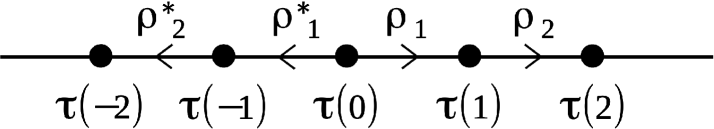
Formulas similar to (2.53)–(2.58) can be easily obtained. The chain of BD transformations is illustrated by Fig. 1.
Let us consider a chain of the forward Bäcklund transformations defined by a sequence of the density functions . A natural question is whether the backward BD transformations can be understood as transformations inverse to the forward ones. More precisely, let be the forward transformation, i.e.,
The question is what density one should assign to a backward transformation in order to come back to , applying it to : . The answer is rather simple and explicit in the case when supports of the functions do not intersect and . In general we have:
| (2.63) |
By assumption, the function has a compact support (which can be a compact domain in or a set of points) such that for all . Let us find the function in the form
where the function has a support and is such that if . We also assume that for all . With these assumptions, equation (2.63) acquires the form
| (2.64) |
The integral in can be transformed by taking “by parts” and using the formula
In this way we get:
| (2.65) |
The first integral in the right-hand side vanishes because on . In fact, under our assumptions the the second integral also vanishes. To see this, we use the explicit formula (2.50) in which we put :
| (2.66) |
After some transformations, we find:
where
Plugging this into (2.65), we get:
because the supports of the functions and do not intersect by the assumption. Finally, we have from (2.64):
| (2.67) |
where
is an irrelevant -independent common multiplier.
2.4 Several chains of BD transformations as a discrete integrable hierarchy
Let us now consider several infinite chains of BD transformations. We begin with two chains in the forward direction that are defined by fixing two sequences of functions and . Starting from an initial KP tau-function , one can apply the first transformation times and then the second one times. We denote the resulting tau-function as . Let us denote the first and the second transformations by and :
| (2.68) |
There are two ways to obtain from (first apply , then or vice versa):
Writing the two composite transformations explicitly, one can easily see that the results differ by a sign, i.e., the anti-commutation relation
| (2.69) |
holds true. Therefore, given , the function is defined only up to a sign444However, since the BA functions are ratios of two tau-functions, the two transformations , commute when they act to the BA functions..
Remark. The anti-commutation relation (2.69) becomes obvious in the realization of the BD transformations via free fermions (section 4.1.3 below).
In order to fix this uncertainty and make to be a well-defined single-valued function on the lattice, we proceed in the following way. Consider a set of chains of the forward BD transformations defined by the operators with sequences of functions , . Let (where all ) be a point of the lattice , and be the vector whose -th component is 1 and all other components are equal to 0. Then we write, by definition:
Let us fix the linear order in the set of the transformations according to the natural order in the set . Then, given , we can uniquely define for as follows:
| (2.70) |
where if and if . This prescription allows one to unambiguously extend the tau-function to all points of the lattice, starting from a given tau-function at the origin .
Let us now derive equations which connect the tau-functions at different points of the -dimensional lattice, as functions of . First, we have the equation
| (2.71) |
where we use the short-hand notation introduced in section 2.1. It can be obtained using the integral formulas of the type (2.68) and bilinear equation (2.5) for the KP tau-function. In order to write this equation in a more compact form, we can use even more short-hand notation like , , etc. Then equation (2.71) acquires the form
| (2.72) |
Tending , we obtain in the limit:
| (2.73) |
Using the short-hand notation from section 2.1 and the ones introduced in the present section, we can write equation (2.28) in the form
| (2.74) |
Put , then the BA function can be represented as , and equation (2.74) can be read as a linear equation for the BA function:
| (2.75) |
Subtracting it from the similar equation for another BD flow with , we get:
The right-hand side can be simplified with the help of equation (2.72). Then this relation becomes the following linear equation for the BA function:
| (2.76) |
Let us mention a slightly different form of this equation which may be useful for applications. Put , , then (2.76) can be written as
| (2.77) |
which means that is obtained from by the action of the first order difference operator acting to it with respect to the variable .
There also exists an equation containing only shifts of the “Bäcklund-Darboux variables” . Let be any cyclic permutation of indices . We need the integral formulas of the type (2.68) for , , and the formulas
that follow from them. Taking into account the bilinear equation (2.5) for the KP tau-function, it is not difficult to see that the equation
| (2.78) |
holds true. In the more explicit notation it reads
| (2.79) |
In particular, we have:
| (2.80) |
Let us note that equation (2.78) is the compatibility condition for the linear problems of the form (2.76). With the help of the same method that was used in section 2.1 to prove that equations of the form (2.5) imply equations (2.4), one can show that equations of the form (2.78) imply the following equations:
| (2.81) |
Finally, we note that equation (2.79) is the equation of the multi-component mKP hierarchy [46] restricted to the sector of discrete variables. To see this, we recall that the tau-function of the -component mKP hierarchy depends on discrete variables and on infinite sets of continuous variables
The integral bilinear equation for the tau-function has the form [46]
| (2.82) |
where the notation means that the times from the set are shifted as in (2.3) and all other times are untouched. The sign factors are defined as follows:
| (2.83) |
Equation (2.82) is valid for all and such that for all . Putting and , where (and also ), we see that the sum in left-hand side of (2.82) has only three non-zero terms (for ), and the integrals are calculated by taking residues at infinity. Then it is not difficult to see that the resulting 3-term bilinear equation is equivalent to (2.79).
2.5 The discrete Schwarzian KP hierarchy
The Schwarzian form of the KP hierarchy is obtained if one chooses the Baker-Akhiezer kernel (BA kernel) as the dependent variable. The BA kernel is the function
| (2.84) |
Moreover, for any integer one can define “higher” (multi-point) BA kernels via
| (2.85) |
where determinant of the Cauchy matrix in the right-hand side is
| (2.86) |
We note the following determinant formula:
| (2.87) |
The proof can be found in [43].
Using the definition and the bilinear equation (2.4), one can prove, after some simple calculations, that the following identity holds:
| (2.88) |
In particular, tending , we obtain a simpler identity:
| (2.89) |
which we will use in what follows. In the short-hand notation it can be written as
| (2.90) |
where , etc.
In the same way as we have defined the wave functions, one can obtain from the BA kernel a more general object, integrating it in and with the functions , :
| (2.91) |
Integrating both sides of (2.90) in and , we obtain the following identity for :
| (2.92) |
Writing it for and shifting the arguments appropriately, we obtain the relations
and
Combining them, we can exclude the wave functions and obtain the equation which contains only -functions:
| (2.93) |
It is easy to check that it can be rewritten in the form
| (2.94) |
Equation (2.93) (or (2.94)) is the discrete Schwarzian KP equation. Its interesting geometric meaning meaning was clarified in the seminal papers [12, 13]. It is also suggestive to compare this equation with (2.34).
The form (2.93) makes it almost obvious that this equation is invariant under fractional-linear (Möbious) transformations
| (2.95) |
It is enough to check this for the three transformations , and , because the general transformation from the Möbious group can be represented as a composition of these three.
Note also that equation (2.94) does not contain the “lattice spacing” parameters explicitly. That is why this equation is actually invariant with respect to any permutations of the discrete variables .
Combining the equations of the form (2.93) written for any triple of distinct indices from the set , one arrives at the equations
| (2.96) |
where the indices in the right-hand side are understood to be taken modulo . These equations can be regarded as the higher equations of the discrete Schwarzian KP hierarchy. Since all of them follow from (2.93), the latter is not only the integrable discretization of the Schwarzian KP equation, but also of the whole hierarchy.
The continuum limit of equation (2.93) is most easily taken in three steps. At the first step we tend keeping the other two parameters fixed. This gives:
| (2.97) |
At the second step we tend and expand equation (2.97) in inverse powers of . The first non-vanishing term arises at . After some calculation this limit yields:
| (2.98) |
where the difference operator is defined as
Finally, one should tend in (2.98). After a relatively long calculation, the first non-vanishing term yields the equation
| (2.99) |
where
| (2.100) |
is the Schwarzian derivative, and we have denoted , , . This is the continuous Schwarzian KP equation in the which first appeared in [44] in the context of Painlevé analysis as the singularity manifold equation associated with the KP equation. Since it was obtained from equation (2.93), it is invariant under the fractional-linear transformations (2.95) by construction. This fact can be also checked directly from equation (2.99). Indeed, the Schwarzian derivative is known to be invariant, and invariance of the other terms can be easily checked for the transformations , and .
Representing the -function as
| (2.101) |
one can show that the transition is a BD transformation, i.e. is another solution of the KP hierarchy. This can be proved in the following way. From (2.88) it follows that
Plugging here (2.38), (2.42) and (2.101), we obtain the relation
where may take values . The three equations in the matrix form can be written as the following linear system for :
The skew-symmetric matrix in the left-hand side is degenerate, and the eigenvector with zero eigenvalue is . Therefore, for existence of nonzero solutions this vector must be orthogonal to the vector in the right-hand side, i.e., the relation
holds. If , it reads
Let be any cyclic permutation of , then writing these equations for with the overall shift , multiplying both sides by and summing the results over the three cyclic permutations, we obtain the 3-term bilinear equation for .
The BD transformation is known in the literature as the binary BD transformation. From (2.84) and (2.91) one can represent the tau-function explicitly as a double integral:
| (2.102) |
It easy to see that any binary BD transformation can be represented as a composition of one forward and one backward BD transformations , introduced in section 2.3.
3 Equations of the BKP type
This section is devoted to the BKP hierarchy, its discrete version and BD transformations. The general references are [17], see also [48]–[51].
3.1 The BKP hierarchy and its discretization
The set of independent variables of the BKP hierachy is the infinite set , where the times carry only odd indices555In this section, we denote the set of times by the same bold letter as for the KP hierarchy and hope that this will not cause any misunderstanding since the KP hierarchy will not be discussed in this section..
Let be the tau-function of the BKP hierarchy. The generating bilinear equation for the BKP tau-function has the form
| (3.1) |
where
| (3.2) |
| (3.3) |
and is a big circle around . This equation is valid for all and . Note that in the BKP case .
Choosing in a special way, one can derive from (3.1) various bilinear equations of the Hirota-Miwa type. For any integer and distinct points set
With this substitution, the residue calculus converts equation (3.1) into the following form:
| (3.4) |
In particular, at we have the equation
| (3.5) |
where
| (3.6) |
Note that the simplest solution is . This follows from the easily verified identity
Equation (3.5) first appeared in the work [36]. As is proved in [43], it is in fact equivalent to the whole BKP hierarchy.
Equation (3.5) can be also understood as a fully discrete BKP equation. For any function set
| (3.7) |
similarly to (2.6), and employ the same short-hand notation as in (2.7). Then equation (3.5) acquires the form
| (3.8) |
As in the KP case, if one considers this equation as a discrete one, without any concern about analytic properties of solutions, values of the coefficients are not that important because they can be made arbitrary by means of the simple transformation given in section 2.1.
The higher functional relations of the BKP hierarchy (BKP analogs of equations (2.45) and (2.46)) were derived in the work [43] as corollaries of equations (3.4). In the most general and suggestive form, they can be written in terms of Pfaffians of the skew-symmetric matrices (3.6) and
| (3.9) |
in the following way:
| (3.10) |
Some information about Pfaffians is collected in Appendix A. The Pfaffian downstairs can be explicitly evaluated:
| (3.11) |
and regarded as a Pfaffian analog of the Vandermonde determinant. Equation (3.10) is written for an even number of the points . To obtain a similar eqiuation for an odd number of them, equal to , one should simply tend in (3.10) to . In this limit, the skew-symmetric matrices still remain to be of size but the matrix elements and become equal to . In particular, equation (3.5) is the simplest particular case of (3.10) corresponding to the choice , .
The BA function is defined by the formula
| (3.12) |
Note that the dual BA function, if defined as in (2.20), is just and thus is not an independent function. In fact another definition of the dual BA function is possible (with the help of the dressing operator; see, for example, [51]) but it also gives a function that is not independent from the function defined by equation (3.12). As in the KP case, the BA function satisfies linear equations. The simplest one follows from equation (3.5) rewritten in a special way. Namely, set , then, using the definition (3.12), one is able, after some simple transformations, to represent equation (3.5) in the form of a linear difference equation for the BA function. In the short-hand notation it reads:
| (3.13) |
Note that comparing to the analogous equations (2.30) for the discrete KP hierarchy it has four terms, rather that three, associated with four vertices of a plaquette of the square lattice.
Like in the KP case, the BA function depends on the spectral parameter , and enters the -independent equation (3.13) linearly. This allows one to introduce a general solution to the linear equation (3.13) in the same way as in (2.22), i.e., by integrating the BA function with an arbitrary function (or a distribution) of :
| (3.14) |
(Again, we assume that has a compact support.) So, the function satisfies the linear equation (3.13):
| (3.15) |
The BA function is just one special solution of this equation.
Equations of the form (3.15) written for each pair of the discrete variables form an overdetermined linear system whose compatibility condition is just the bilinear equation (3.8). To see this, we rewrite (3.15) in the form
| (3.16) |
for () and shift the third variable (which is the same in all terms in (3.16)) by 1: . (As before, is any cyclic permutation of .) Then (3.16) reads
| (3.17) |
Compatibility of the three equations (3.16) means that
| (3.18) |
Expressing and in the right-hand side of (3.17) through with the help of equations (3.16), and substituting the results into (3.18), one can see that cancels from these equalities while the other terms give the compatibility conditions
| (3.19) |
where
Therefore, the compatibility requires that . This is precisely equation (3.8).
3.2 The discrete modified BKP hierarchy
Our next goal is to derive an equation that would contain the -functions at neighboring points of a 3D lattice only, such that the tau-function does not participate in it explicitly. It is thus going to be a BKP analogue of the discrete mKP equation (2.32), and by analogy, might be called the discrete modified BKP (mBKP) equation. However, we will see that the form of this equation suggests to simultaneously regard it as a BKP analogue of the discrete Schwarzian KP equation (2.93). To derive it, we fix three parameters , with the associated discrete variables being , and write equation (3.15) for each pair of indices in the form
| (3.20) |
Let be any cyclic permutation of the indices . Shifting in (3.20) (with ), it is easy to observe that the combination
is symmetric with respect to all permutations of the indices. Therefore, we obtain the discrete equations for the -function of the form
| (3.21) |
or
| (3.22) |
Discrete equations of this form first appeared in [13], where their geometric meaning was also clarified. It is easy to see that they are invariant under fractional-linear (Möbius) transformations of the form (2.95). Therefore, they can be simultaneously regarded as BKP analogues of the discrete mKP equation (because they are written for the wave functions, like in the mKP case) and of the discrete Schwarzian KP equation (because they are invariant under the Möbius transformations). It should be also noted that these equations do not contain the ”lattice spacing” parameters explicitly, and hence should be invariant under any permutation of the variables . Indeed, under the permutations, the two equations in (3.22) are transformed into each other. So, for the BKP hierarchy we have two equations for one and the same function rather than one. However, as it follows from the construction, these equations are compatible and have a lot of common solutions.
3.3 Continuum limit of the discrete modified BKP equation
As before, the continuum limit of equations (3.22) should be taken in steps. At the first step we tend keeping the other two parameters fixed. This gives:
| (3.23) |
where . The further limit as is obtained by expansion of these equations up to the first non-vanishing order in . The two equations in (3.23) give the same result:
| (3.24) |
Finally, we tend in (3.24). To obtain a non-trivial equation from (3.24) in this limit, one should expand the both sides up to the order . The necessary calculations are direct but rather long. In the variables the equation reads:
| (3.25) |
where is the Schwarzian derivative given by (2.100). Let us mention that
where prime means the -derivative. The Möbius-invariance of equation (3.25) can be directly verified. As was already mentioned, equation (3.25) is simultaneously the Schwarzian analog of the BKP equation.
3.4 Bäcklund-Darboux transformations
Equation (2.38) suggests to define BD transformations for the tau-function of the BKP hierarchy following the analogy with the KP case. To wit, let us represent a solution to the linear equation (3.15) in the form
| (3.26) |
where is the BD-transformed tau-function (below we shall see that it is a BKP tau-function indeed). From (3.14) we see that
| (3.27) |
To prove that is a BKP tau-function (i.e. that it obeys equation (3.8) if does so), we substitute (3.26) into equation (3.15). After cancellations, we obtain the following equation connecting and :
| (3.28) |
As before, let be any cyclic permutation of the indices . For any cyclic permutation, write the equation of the form (3.28):
| (3.29) |
and multiply its both sides by . Summing the three equations obtained in this way, we arrive at the relation
| (3.30) |
In a similar way, multiplying the both sides of (3.29) by and summing the resulting equations, we arrive at
| (3.31) |
Next, we proceed by shifting in (3.29) which results in
| (3.32) |
Multiplying both sides of this relation by and summing the resulting equations, we get
| (3.33) |
At last, multiplying the both sides of (3.32) by and summing the three equations, we obtain the relation
| (3.34) |
Now, equation (3.8) states that the right-hand side of (3.31) (and, therefore, its left-hand side as well) is equal to
Comparing with (3.33), we see that it holds
which is the four-term bilinear equation (3.8) for the BKP tau-function. We have proved that the transformation of the form (3.27) sends any solution to the BKP hierarchy to another solution, i.e., it is indeed a BD transformation.
Similarly to the KP case, given a sequence of functions , we can repeat the transformation of the form (3.27) many times, defining the chain of BD transformations by the recursion relation
| (3.35) |
Equation (3.28) for the chain can be written in the form
| (3.36) |
where . Remarkably, equation (3.36) has essentially the same structure as the four-term bilinear equation (3.8) for the BKP tau-function666Values of the numerical constants in front of each term are different in these equations but this discrepancy is not that very important since they can be changed by a simple redefinition of the tau-function that consists in multiplying it by exponential function of a quadratic form in the independent variables.. Namely, the discrete “variable” that numbers sequential steps of the BD chain in equation (3.36) enters in the same way as the third discrete variable in (3.8).
The BD transformations, as defined above, are of the forward type. A crucial difference, comparing to the KP case, is that any analogs of backward transformations do not exist in the BKP setup. There exist different possibilities to extend the chain to the backward direction so that equation (3.36) remains valid. The simplest one is to put for all . Note, however, that equation (3.36) is invariant under the change . Therefore, we can extend the chain to the backward direction in the symmetric way by putting for , or for .
Explicitly solving recurrence relation (3.35), we have:
| (3.37) |
which is valid for both even and odd . With the help of equation (3.10), the right-hand side can be expressed in terms of the Pfaffian:
| (3.38) |
where the skew-symmetric matrix is defined in (3.10), i.e.,
| (3.39) |
and for brevity we have denoted This is the BKP analogue of equation (2.52). Equation (3.38) is written for with an even non-negative but can be easily adopted for the case of an odd . For this, one should omit the terms in the exponential factors and formally put equal to the (formal) delta-function with support at infinity after that. Informally, this means that one should put in the matrix . The skew-symmetric matrix under Pfaffian is still of size but the elements and are represented as single integrals with the density functions , respectively rather than double ones.
Let us mention some important particular cases of equations (3.37) and (3.38). They simplify considerably if the initial tau-function is taken to be the trivial solution, i.e. if one puts . In this case , and (3.38) reads
| (3.40) |
The special choice , where the distribution is the delta-function concentrated on the ray , and is some continuous function, converts the multiple integral in (3.37) to
| (3.41) |
This is the partition function of the Bures statistical ensemble whose connection with the BKP hierarchy was addressed in [54] in some details. Equation (3.40) specialized to this case reads:
| (3.42) |
where . For odd this formula needs some modifications. The details can be found in [54]. Applications to Pfaffian point processes were discussed in [55].
Choosing the density functions in (3.37) (with ) to be distributions concentrated at a finite number of distinct isolated points in , one obtains multi-soliton solutions to the BKP hierarchy and their generalizations. For example, one may take
| (3.43) |
Here we will not go into further details. For the construction of the soliton solutions to the BKP hierarchy in terms of Pfaffians see [56, 57].
3.5 Two and three chains of the Bäcklund-Darboux transformations
Let us consider two BD transformations , with the density functions with supports on some compact domains , respectively. Applying first , then , we have:
| (3.44) |
Because of the singularity at the order of integrals in general can not be interchanged. However, if we require that
| (3.45) |
then the singularity is absent, the integrals over and can be interchanged, and we see that the opposite order of the transformations (first , then ) gives the same result as in (3.44) but with sign minus. So, in this case the transformations anticommute: . This (anti)commutation law receives its natural interpretation in the fermionic construction based on neutral Fermi-operators (see section 4.2 below).
Now, given sequences of density functions , such that their supports satisfy the conditions for all 777To satisfy these conditions, it is enough to assume that the supports belong to the right upper quadrant of the complex plane which we denote as ()., we can consider chains of the BD transformations in the way explained in section 2.4. In the similar way, we can introduce discrete variables that count the number of BD transformations made in the “th direction”. Below we use the short-hand notation introduced in that section: etc. for the tau-functions obtained by sequential application of different BD transformations. Using the integral representation of the BD transformations and the basic bilinear equation (3.8), it is not difficult to obtain the following equations:
| (3.46) |
| (3.47) |
The last equation has the same structure as the basic bilinear equation (3.8), but with different coefficients equal to . This equation should be compared with the equation for the tau-function of the multi-component BKP hierarchy888Its construction was very briefly outlined in [17] and requires more attention..
4 The approach based on free fermions
A very instructive and suggestive approach to integrable hierarchies such as KP and BKP is the operator technique based on the quantum field theory of free massless fermions. It was suggested in the works by Kyoto school in 1983 [15, 16]. In particular, the approach based on free fermions allows one to represent the BD transformations in a very simple and clear form, making all statements related to them almost obvious.
4.1 Charged fermions (KP)
Let us begin with a brief remainder of how the KP hierarchy looks like in terms of free fermions. For more details see the original papers [15, 16] and the detailed review [52].
4.1.1 The algebra of Fermi-operators and vacuum states
Let , , be free Fermi-operators with the standard anti-commutation relations
| (4.1) |
The Fermi-operators carry a charge: the charge of is and the charge of is . They generate an infinite dimensional Clifford algebra . Elements of the algebra are linear combinations of all possible products of the charged Fermi-operators , with different indices (monomials). They are multiplied in accordance with the anticommutation relations (4.1).
We will also use the generating series of the Fermi-operators defined as
| (4.2) |
They are fermionic operator fields in the complex plane of the variable .
Next, we introduce the right vacuum state as a “Dirac sea”, where all negative mode states are empty and all non-negative ones are occupied:
Similarly, the dual (left ) vacuum state has the properties
With respect to the vacuum , the operators with and with are annihilation operators while the operators with and with are creation operators (the latter ones create holes). We also need “shifted” Dirac vacua and defined as
| (4.3) |
| (4.4) |
This definition implies that the charge of the right vacuum is , and the charge of the left vacuum is .
The vacuum expectation value is a Hermitian linear form on the Clifford algebra fixed by the normalization Then, from the commutation relations (4.1) and definitions of the “shifted” Dirac vacua (4.3), (4.4) it follows that for any . Bilinear combinations of fermions satisfy the properties for all and
The expectation value of any operator with non-zero charge is zero. As is well known, the expectation values of products of Fermi-operators with zero charge can be determined by various forms of the Wick theorem (see [52] for details). For example, we have:
| (4.5) |
where
| (4.6) |
(assuming that ).
Neutral bilinear combinations of the Fermi-operators, with certain conditions on the matrix , generate an infinite-dimensional Lie algebra [16]. Exponentiating such expressions, one obtains an infinite dimensional group (a version of ). Elements of this group can be represented in the form
| (4.7) |
Following the paper [52], we call them (invertible) group-like elements. Their main property is the following commutation relations with the - and -operators:
| (4.8) |
where the matrix is .
4.1.2 The KP tau-function as an expectation value
Consider the following bilinear operators with zero charge:
| (4.9) |
They play especially important role in the applications to the integrable hierarchies of the KP type. These operators are positive Fourier modes999The precise definition requires a normal ordering, which is not essential for the operators (4.9) with , see [52]. of the “current operator” which is given by the (normally ordered) product of the Fermi-fields: . It is easy to see that , . Let be the set of parameters which are going to be the KP times. Set
| (4.10) |
It is not difficult to prove that
| (4.11) |
where is given by (2.2).
As it has been established in the works of the Kyoto school, the expectation values of group-like elements are -functions of integrable hierarchies of nonlinear differential equations, i.e., they obey an infinite set of bilinear equations of the Hirota-Miwa type [47, 36] which eventually follow from the Wick theorem for expectation values of products of the Fermi-operators.
The KP tau-function is defined as the vacuum expectation value
| (4.12) |
where is any group-like element of the form (4.7) (or of a more general form given below). The mKP tau-function is defined as
| (4.13) |
For each it is also a KP tau-function as a function of the times . The proof that the functions having this form satisfy the bilinear relation of the KP hierarchy in the generating integral form (2.1) is based on the operator bilinear identity
| (4.14) |
or
| (4.15) |
which is valid for the group-like elements with zero charge of the form (4.7) (and also for certain operators with a nonzero charge of a more general form given below). The identities (4.14), (4.15) immediately follow from the commutation relations (4.8). Equation (4.14) is to be understood as the identity
| (4.16) |
valid for any states , , , from the fermionic Fock space. Choosing , , , we see that the right-hand side of (4.16) vanishes, and the rest can be written as
| (4.17) |
To bring it to the form (2.1), one should use the commutation relations (4.11) and the bosonization rules
| (4.18) |
(equations (2.93) in [52]). Note that the charge of both sides are and in the first and the second equation respectively. The repeated use of the rules (4.18) gives more general bosonization formulas:
| (4.19) |
where is the Vandermonde determinant given by (2.12).
The BA functions (2.20) are expressed through the vacuum expectation values by the following formulas:
| (4.20) |
The BA kernel (2.84) is given by
| (4.21) |
It is assumed in (4.20), (4.21) that the element has zero charge. To see that these representations agree with formulas (2.20) and (2.84), one should use the bosonization rules.
Along with KP tau-functions given by (4.12) with of the form (4.7) more general KP tau-functions can be introduced as expectation values of certain fermionic group-like operators with a definite nonzero charge. In [52] such operators are called non-invertible group-like elements. To wit, let be a linear combination of the operators and be a linear combination of the operators . The element
has charge . The operator as well as the product with of the form (4.7) are examples of non-invertible group-like elements of charge . Although neither nor satisfy (4.8), it is easy to check that they nevertheless obey the basic bilinear operator identity (4.14), which is enough for derivation of the bilinear equation for the tau-function. With the help of it, it is not difficult to show (see, e.g. [52]) that the function
| (4.22) |
is a KP tau-function, too. In the corresponding expressions for the BA functions the left vacuum should be shifted accordingly, to make the whole expression (including the vacua and the Fermi-operators) neutral.
4.1.3 The BD transformations
Using the representation (4.22) of KP tau-functions, it is easy to define the BD transformations. Introduce the operators
| (4.23) |
where and are density functions, as in (2.22). The forward BD transformation that sends the tau-function (4.12) to given by (2.41) is defined as
| (4.24) |
Hereafter we assume that the element has zero charge; otherwise the left vacuum should be shifted accordingly. Similarly, the backward BD transformation from to is given by
| (4.25) |
A chain of the BD transformations is defined by sequential action of the operators of the form (4.23). Namely, introduce the operators
| (4.26) |
then the tau-function (2.50) and (2.60) can be represented as
| (4.27) |
and
| (4.28) |
This is easy to see with the help of bosonization formulas (4.19). One can also consider a composition of forward and backward BD transformations:
| (4.29) |
The representation of BD transformations in terms of Fermi-operators makes it obvious that any two forward and any two backward transformations anticommute while a forward transformation anticommutes with a backward one only if supports of the corresponding density functions do not intersect (because in this case anticommutes with ). The case in (4.29) corresponds to a composition of sequential binary BD transformations, and the Wick theorem implies that the right-hand side of (4.29) in this case is the determinant of the matrix whose matrix elements are the BA kernels at different points, as in equation (2.87).
4.2 Neutral fermions (BKP)
The BKP hierarchy, like the KP one, admits a description in terms of free massless fermions. However, in this case we need neutral fermions , and the corresponding neutral fields
This formalism was developed in [16, 17]. In our presentation, we also follow the work [53].
4.2.1 The algebra of neutral Fermi-operators and vacuum states
The neutral Fermi-operators satisfy the anticommutation relation
| (4.30) |
We thus see that for all . The operator is special: its square is nonzero. At we have from (4.30):
The algebra of neutral fermions consists of linear combinations of all possible products of the neutral Fermi-operators (monomials). Elements of the algebra are multiplied in accordance with the anticommutation relations (4.30). One can define parity of some elements of the algebra by the following rules:
and
for any two elements with a definite parity. For the neutral Fermi-operators, parity is a characteristic analogous to charge for the charged ones. Elements with will be called , and those with even. Any element of the algebra can be represented as a sum of even and odd elements.
The right and left vacua can be defined by the requirements
| (4.31) |
However, these properties do not yet fix the vacuum states uniquely, because given vacuum states , the states and also satisfy conditions (4.31). One of possibilities to choose the vacuum states is using the embedding of the algebra into the Clifford algebra of charged fermions and identify the vacuum state and its dual with the right and left Dirac vacua for the latter111111This is done in detail, e.g., in [53].. Here we adopt this “physical” point of view. Some details are given in Appendix B of the present paper. For a more detailed (and more rigorous) treatment of the algebra and the vacuum states see [17].
Assuming that the right and left vacuum states are fixed, we define the vacuum expectation value by the properties that a) for all odd and b) for even elements it holds
| (4.32) |
We note that
for any . In fact the explicit form of the right-hand sides of (4.32) follows from the anticommutation relations (4.30) and conditions (4.31). For monomials of a higher even degree, the expectation values can be found using the Wick theorem. Let be linear combinations of the Fermi-operators , then it holds:
| (4.33) |
where the sum goes over all permutations of the set such that
and is the signature of the permutation .
In particular, we have:
| (4.34) |
and multi-point correlation functions of the neutral fields are given by the Pfaffian of the skew-symmetric matrix
| (4.35) |
We have from (4.34):
and it follows from the Wick theorem (4.33) that
| (4.36) |
The Pfaffian can be explicitly found (see (3.11)), and the result is
| (4.37) |
Bilinear combinations of the neutral Fermi-operators, with certain conditions on the matrix , which we will not discuss here, generate an infinite-dimensional Lie algebra [16]. Exponentiating these expressions, one obtains an infinite dimensional group. Elements of this group can be represented in the form
| (4.38) |
with a skew-symmetric matrix . (Without loss of generality, its diagonal elements can be put equal to zero.) By analogy with (4.7) we call them group-like elements.
4.2.2 The BKP tau-function as an expectation value
Consider the following even bilinear operators:
| (4.39) |
It is easy to see that for all even nonzero . Let be the set of parameters which are going to be the BKP times. Set
| (4.40) |
It is not difficult to prove that , hence
| (4.41) |
where is the same as in (3.2). We also note that , and hence .
Along with elements of the form (4.38) it is necessary to consider elements of the following more general form:
| (4.42) |
where are linear combinations of the Fermi-operators . General BKP tau-functions are given by
| (4.43) |
with of the form (4.42). The proof that such functions satisfy the bilinear relation of the BKP hierarchy in the generating integral form (3.1) is based on the operator bilinear identity
| (4.44) |
which is valid for the group-like elements of the general form (4.42) and also for elements of the form (4.42). Equation (4.44) is to be understood as the identity
| (4.45) |
valid for any states , , , from the fermionic Fock space for neutral fermions. Choosing , , , we have from (4.45):
or
To bring this equation to the form (3.1), one should use the “neutral” analogs of bosonization rules (4.18):
| (4.46) |
(see equations (6.5) in [16]). Note that the second equation here can be rewritten in a form which does not contain the pre-factor , and thus looks closer to the first equation:
| (4.47) |
where . By induction, one can prove the following more general bosonization formulas:
| (4.48) |
where . Acting by both sides of the first formula to the right vacuum , we reproduce (4.37).
The BA function is expressed as follows:
| (4.49) |
To see that it is indeed connected with the tau-function in the same way as in (3.12), one should use the bosonization rules.
4.2.3 The BD transformations
Consider the operator
| (4.50) |
where is the same function (or distribution) as in (3.14). Using this operator, the BD transformation (3.27) for the BKP tau-function can be represented as
| (4.51) |
that is easy to check. The fact that is a BKP tau-function, too, is clear because the right-hand side of (4.51) has the form (4.43).
To define a chain of sequential transformations of this type,
we fix some half-infinite sequence of density functions and introduce the operators
| (4.52) |
Equation (4.51) is then rewritten as
| (4.53) |
with . The next tau-function then is
| (4.54) |
For general positive , we have:
| (4.55) |
Note that for even and for odd . One can easily check that the right-hand side of (4.55) coincides with (3.37). From the representation (4.55) it is clear that, in contrast to the case of charged fermions, any two BD transformations in general do not anticommute (a sufficient condition for anticommutativity of two transformations , is empty overlap between supports of and ).
4.2.4 BD transformations for BKP versus those for KP
It is known that the BKP tau-functions are square roots of certain KP tau-functions in which all “even” times are put equal to 0. This fact allows us to connect the BD transformations for these two hierarchies. The connection can be most easily established using the technique of free fermions. Specifically, we need the embedding of the algebra of neutral fermions into the Clifford algebra of the charged ones. This realization of the algebra is described in Appendix B. In this section we use the notation and definitions from Appendix B.
The important fact that allows one to connect tau-functions for the KP and BKP hierarchies is that that the operators , commute with , . To wit, let be a BKP tau-function:
| (4.56) |
where
| (4.57) |
with some density functions or distributions with supports in the right upper quadrant. This tau-functions can be thought of as the result of sequential BD transformations for the BKP hierarchy. The same representation holds with the algebra of the -operators in the right-hand side. Then we can write:
| (4.58) |
where . The product can be transformed using the formulas from Appendix B:
| (4.59) |
Therefore, we conclude that
| (4.60) |
where
| (4.61) |
and
| (4.62) |
Plugging this into (4.58), we conclude that
| (4.63) |
This means that the BKP tau-function is the square root of the KP tau-function corresponding to the group-like element , with all even times being put equal to 0. The insertion implements the binary BD transformation of the KP tau-function, with special density functions given by (4.62). Therefore, any BD transformation of the BKP type is equivalent to a binary BD transformation of the KP type with specially chosen density functions, as in (4.62).
5 Conclusion
In this paper, we have revisited the world of Bäcklund-Darboux (BD) transformations for integrable hierarchies of nonlinear partial differential equations such as KP, mKP, BKP and their difference analogs. We have tried to develop a unified approach based on the bilinear formalism, where the main hero is the tau-function. We have seen that when iterated, the BD transformations form infinite or half-infinite chains, with th step of the chain being defined with the help of a density function (which can be a distribution). Remarkably, neighboring members of such a chain are connected by bilinear equations belonging to the same hierarchy (more precisely, to its discrete analog), whose form does not depend on a particular choice of the density functions at each step.
In conclusion, let us note that for some important applications, the chains of sequential BD transformations (finite or infinite) are of a special interest. The most important and interesting cases of the whole construction are the cases when the density functions have supports concentrated either on 1D lines (such as, for example, or ) or at some distinct points in , i.e., when they are distributions rather than continuous functions in the plane.
The former possibility, when the density corresponding to each step of the BD chain is concentrated on 1D curves in the 2D plane, is relevant to the integrable properties of the theory of random matrices121212The literature on random matrices is enormous. Here we only mention the classical book [59], where the connections with integrable equations were not discussed, and the papers [60, 61, 62, 63] devoted to integrability of models of random matrices.. In known examples, the curves are either the real line for matrices with real eigenvalues (or in some cases) or the unit circle for unitary matrices. In these applications, the discrete variable numbering sequential steps of the BD chain is just size of the random matrices. In this case the chain of BD transformations is half-infinite, and for applications to quantum gravity and string theory of particular interest is the limit taken in one or another sophisticated way (for example, the double-scaling limit).
Meanwhile, integrable properties of random matrices with complex eigenvalues (for example, normal matrices) require an access to a similar theory of BD transformations for more general integrable hierarchies such as 2D Toda lattice. We hope to address this issue in a separate publication.
The applications to quantum integrable models arise in the cases when the density functions corresponding to the BD transformations are concentrated at some isolated points in chosen in a special way such that the tau-functions at each level of the BD chain are polynomials or “trigonometric polynomials” of the first variable identified with the quantum spectral parameter (for quantum models with rational and trigonometric -matrices respectively). Unlike the applications to matrix models, of the main interest here are finite chains of BD transformations, with the discrete variable varying from to , where the comes from the underling symmetry algebra of the quantum model ( or ). Another difference is that the BD transformations of the chain should be performed in the backward direction, from to , thus “undressing” the original problem to the trivial one. The sequential steps of the chain correspond to the levels of the nested Bether ansatz procedure. Given a fixed as a polynomial (or trigonometric polynomial) whose roots are inhomogeneity parameters of the spin chain, the procedure of undressing it to the trivial one compatible with the mKP hierarchy, has a finite number of solutions, each of which corresponding to different eigenstates of the quantum spin chain (on a finite 1D lattice). Details on this procedure can be found in [19].
As we have seen in section 2.3, there are two types of BD transformations for the mKP hierarchy: forward and backward ones. The scheme outlined in the previous paragraph is related to the forward transformations which appear as avatars of the nested Bethe ansatz for quantum models based on classical symmetry algebras and their -deformations. The results of [27, 28, 34] suggest that for graded quantum magnets (based on superalgebras, for example, one should include into play also the backward BD transformations defined by equation (2.59), with the BD chain consisting of forward and backward transformations. We anticipate that for the operator realization of the BD transformations given in section 4.1.3 might be useful and instructive. We plan to address the details elsewhere.
Last but not least, there is a tempting problem to investigate whether there are some applications of the BD transformations and their chains for the BKP hierarchy (see section 3.4) to any quantum integrable models, in the analogy with the mKP case outlined above. Perhaps, to uncover the connection (if it does exist in one or another form), one should consider generalized quantum spin chains based on symmetry algebras of type B rather than A.
Acknowledgments
I thank J. Harnad whose questions and comments on my recent paper [19] gave me a strong motivation to revisit the world of Bäcklund-Darboux transformations and try to understand them better. Also, it was J. Harnad who drew my attention to the seminal papers [12, 13]. Thanks are also due to A. Orlov and V. Prokofev for valuable discussions. An illuminating discussion with A. Veselov, after which the idea that Bäcklund-Darboux transformations need a better understanding first came to my mind, is also gratefully acknowledged.
This work is an output of a research project implemented as a part of the Basic Research Program at the National Research University Higher School of Economics (HSE University).
Appendix A: Pfaffians
Here we briefly recall some facts about Pfaffians which are necessary for reading sections 3 and 4. More details can be found, e.g., in the book [14].
Odd-dimensional skew-symmetric matrices are degenerate, their determinants are equal to 0. Determinant of an even-dimensional skew-symmetric matrix is always a full square. The Pfaffian of an even-dimensional skew-symmetric matrix is square root of its determinant. It is given by the explicit formula
where the sum is taken over all permutations of the indices such that
and is signature of the permutation. For example, at we have and at . The recurrence relation for the Pfaffians is
where is a skew-symmetric matrix of an even size and is the matrix with the first and th columns and rows removed.
Let be an skew-symmetric matrix with . The following properties of its Pfaffian are useful in applications:
It is known that tau-functions of integrable hierarchies of type A (such as KP and 2D Toda) are determinants (in general case, of infinite-dimensional matrices or operators) while those for hierarchies of types B and D are Pfaffians of some (possibly, infinite dimensional) skew symmetric matrices.
Appendix B: Neutral fermions from the charged ones
It is instructive to realize the algebra of neutral fermions dealt with in section 4.2 as a subalgebra of the Clifford algebra of the charged fermions discussed in section 4.1. This embedding was first suggested in 1983 in the seminal paper [16] and reviewed many times after that. Below we follow the paper [53].
In fact the neutral Fermi operators can be realized in terms of the charged ones in the following way:
| (B1) |
Then it is easy to check that the operators and defined in this way obey the anticommutation relations (4.30) and the -operators anti-commute with the -operators:
| (B2) |
In particular, . For the fermionic fields we have:
| (B3) |
Note that
| (B4) |
Let , be the dual Dirac vacua for the charged fermions introduced in section 4.1. Then it is easy to check that the operators , defined as above act to the vacuum states as follows:
| (B5) |
These formulas allow one to identify the vacuum states , for the charged fermions with the vacuum states , introduced in section 4.2 for the neutral fermions131313We note in passing that the other vacuum state introduced in section 4.2 is .. In our opinion, this identification makes some constructions from section 4.2 less artificial.
We can introduce the group-like elements
| (B6) |
with a skew-symmetric matrix . They are simultaneously serve as group-like elements for the algebra , as well as their product . Moreover, the elements , obviously commute with each other.
An important special case of group-like elements are the “evolution operators” , , where
| (B7) |
and
| (B8) |
Note that for all even positive , so the sums in (B7) can be taken over all , with only times with odd indices entering the game. Moreover, we have
| (B9) |
where in the right-hand side is the evolution operator (4.10) for charged fermions, and it is implied that all times with even indices in the set are put equal to 0.
At last, let us show that the operator bilinear identity (4.44) for neutral fermions follows from the identities (4.14), (4.15) for charged fermions. Using the embedding , we can rewrite (4.44) as
| (B10) |
where is the group-like element from the algebra . After opening the brackets we see that half of the terms cancel due to identities (4.14), (4.15) and what is left is to prove that
| (B11) |
| (B12) |
Of course for arbitrary group-like this does not take place. However, for special of the form which corresponds to solutions of the BKP hierarchy one can prove both (B11), (B12).
Let us present some details for (B11). We need to prove that commutes with in the same way as , i.e.,
or
| (B13) |
Comparing with (4.8), we see that we should prove the following symmetry of the matrix :
| (B14) |
Writing
(where the skew-symmetry of the matrix is used), we conclude that the matrix for the element is of the form
| (B15) |
from which it follows that
| (B16) |
The symmetry (B14) of the matrix is a consequence of this. The proof of (B12) is similar.
References
- [1]
- [2] V.B. Matveev, M.A. Salle, Darboux transformations and solitons, Berlin: Springer, 1991.
- [3] C. Rogers, W. Schieff, Bäcklund and Darboux transformations, Cambridge Texts in Applied Mathematics 30, Cambridge University Press, 2002.
- [4] J.J.C. Nimmo, Darboux transformations and the discrete KP equation, J. Math. Phys. A: Math. Gen. 30 (1997) 8693–-8704.
- [5] J.J.C. Nimmo, R. Willox, Darboux transformations for the two-dimensional Toda system, Proc. R. Soc. Lond. A 453 (1997) 2497–2525.
- [6] J.J.C. Nimmo, W.K. Schief, Superposition principles associated with the Moutard transformation: an integrable discretization of a (2+1)-dimensional sine-Gordon system, Proc. R. Soc. Lond. A 453 (1997) 255–279.
- [7] J.J.C. Nimmo, Darboux transformations for discrete systems, Chaos, Solitons and Fractals 11 (2000) 115–120.
- [8] J. Harnad, Y. Saint-Aubin, S. Shnider, Bäcklund transformations for nonlinear sigma models with values in Riemannian symmetric spaces, Commun. Math. Phys. 92 (1984) 329–367.
- [9] J. Harnad, Y. Saint-Aubin, S. Shnider, The Soliton correlation matrix and the reduction problem for integrable Systems, Commun. Math. Phys. 93 (1984) 33–56.
- [10] L. Bogdanov, B. Konopelchenko, Analytic-bilinear approach to integrable hierarchies: I.Generalized KP hierarchy, J. Math. Phys. 39 (1998) 4683–-4700.
- [11] L. Bogdanov, B. Konopelchenko, Möbius invariant integrable lattice equations associated with KP and 2DTL hierarchies, Phys. Lett. A 256 (1999) 39–-46.
- [12] B. Konopelchenko, W. Schief, Menelaus’ theorem, Clifford configurations and inversive geometry of the Schwarzian KP hierarchy, J. Phys. A: Math. Gen. 35 (2002) 6125–6144.
- [13] W. Schief, Lattice geometry of the discrete Darboux, KP, BKP and CKP equations. Menelaus’ and Carnot’s theorems, J. Nonlinear Math. Phys. 10 (Supplement 2) (2003) 194-–208.
- [14] R. Hirota, Direct methods in soliton theory, Cambridge Tracts in Mathematics, vol. 155, 2004.
- [15] E. Date, M. Jimbo, M. Kashiwara and T. Miwa, Transformation groups for soliton equations: Nonlinear integrable systems – classical theory and quantum theory (Kyoto, 1981), Singapore: World Scientific, 1983, 39–119.
- [16] M. Jimbo and T. Miwa, Solitons and infinite dimensional Lie algebras, Publ. Res. Inst. Math. Sci. Kyoto 19 (1983) 943–1001.
- [17] E. Date, M. Jimbo, M. Kashiwara, T. Miwa, Transformation groups for soliton equations. IV. A new hierarchy of soliton equations of KP-type, Physica 4D (1982) 343–365.
- [18] J. Harnad and F. Balogh, Tau functions and their applications, Cambridge Monographs on Mathematical Physics, Cambridge University Press, 2021.
- [19] A. Zabrodin, Classical facets of quantum integrability, to be published in Proceedings of Beijing Summer Workshop in Mathematics and Mathematical Physics, 2024, arXiv:2501.18557.
- [20] L. Faddeev Algebraic Aspects of Bethe-Ansatz Int. J. Mod. Phys. A10 (1995) 1845–1878.
- [21] M. Gaudin, La Fonction d’Onde de Bethe, Masson, Paris, New York, Barcelone, Milan, Mexico, Sao Paulo, 1983.
- [22] N. Bogoliubov, A. Izergin and V. Korepin, Quantum inverse scattering method and correlation functions, Cambridge: Cambridge University Press, 1993.
- [23] N. Slavnov, Algebraic Bethe Ansatz and Correlation Functions, World Scientific, Singapore, 2022.
- [24] I. Krichever, O. Lipan, P. Wiegmann, A. Zabrodin, Quantum integrable systems and elliptic solutions of classical discrete nonlinear equations, Commun. Math. Phys. 188 (1997) 267–304.
- [25] A. Zabrodin, Discrete Hirota’s equation in quantum integrable models, Int. J. Mod. Phys. B11 (1997) 3125–3158.
- [26] A. Zabrodin, Hirota equation and Bethe ansatz, Teor. Mat. Fys. 116 (1998) 54–100 (English translation: Theoretical and Mathematical Physics 116 (1998) 782–819).
- [27] V. Kazakov, A.S. Sorin, A. Zabrodin, Supersymmetric Bethe ansatz and Baxter equations from discrete Hirota dynamics, Nucl. Phys. B790 (2008) 345–413.
- [28] A. Zabrodin, Bäcklund transformations for difference Hirota equation and supersymmetric Bethe ansatz, Teor. Mat. Fyz. 155 (2008) 74–93 (English translation: Theor. Math. Phys. 155 (2008) 567–584), arXiv:0705.4006
- [29] A. Alexandrov, V. Kazakov, S. Leurent, Z. Tsuboi, A. Zabrodin, Classical tau-function for quantum spin chains, J. High Energy Phys. 09 (2013) 064, arXiv:1112.3310.
- [30] A. Gorsky, A. Zabrodin and A. Zotov, Spectrum of quantum transfer matrices via classical many-body systems, JHEP 01 (2014) 070, arXiv:1310.6958.
- [31] A. Alexandrov, S. Leurent, Z. Tsuboi, A. Zabrodin, The master -operator for the Gaudin model and the KP hierarchy, Nucl. Phys. B883 (2014) 173–223.
- [32] A. Zabrodin, The master -operator for vertex models with trigonometric -matrices as classical tau-function, Teor. Mat. Fys. 174:1 (2013) 59–76 (English translation: Theor. Math. Phys. 174 (2013) 52–67), arXiv:1205.4152.
- [33] A. Zabrodin, The master T-operator for inhomogeneous XXX spin chain and mKP hierarchy, SIGMA 10 (2014) 006, arXiv:1310.6988.
- [34] Z. Tsuboi, A. Zabrodin, A. Zotov, Supersymmetric quantum spin chains and classical integrable systems, J. High Energy Phys. 05 (2015) 086, arXiv:1412.2586.
- [35] E. Date, M. Jimbo and T. Miwa, Method for generating discrete soliton equations I, II, Journ. Phys. Soc. Japan 51 (1982) 4116–4131.
- [36] T. Miwa, On Hirota’s difference equations, Proc. Japan Acad. 58 Ser. A (1982) 9–12.
- [37] E. Date, M. Jimbo, M. Kashiwara and T. Miwa, Transformation groups for soliton equations III, J. Phys. Soc. Japan 50 (1981) 3806–3812.
- [38] V. Kac and J. van de Leur, The -component KP hierarchy and representation theory, in: A.S. Fokas, V.E. Zakharov (Eds.), Important Developments in Soliton Theory, Springer-Verlag, Berlin, Heidelberg, 1993.
- [39] K. Takasaki and T. Takebe, Universal Whitham hierarchy, dispersionless Hirota equations and multicomponent KP hierarchy, Physica D 235 (2007) 109–125.
- [40] L.-P. Teo, The multicomponent KP hierarchy: differential Fay identities and Lax equations, J. Phys. A: Math. Theor. 44 (2011) 225201.
- [41] I. Krichever, A. Zabrodin, Quasi-periodic solutions of the universal hierarchy, Annales Henri Poincare (2024), arXiv:2308.12187.
- [42] K. Takasaki, T. Takebe, Integrable hierarchies and dispersionless limit, Rev. Math. Phys. 7 (1995) 743–808, arXiv:hep-th/9405096.
- [43] Y. Shigyo, On addition formulae of KP, mKP and BKP hierarchies, SIGMA 9 (2013) 035.
- [44] J. Weiss, The Painlevé property for partial differential equations: II. Bäcklund transformations, Lax pairs and Schwarzian derivative, J. Math. Phys. 24 1405–-1413.
- [45] F. Nijhoff, H. Capel, The direct linearisation approach to hierarchies of integrable PDEs in 2+1 dimensions: I. Lattice equations and the differential-difference hierarchies, Inverse Problems 6 (1990) 567–590.
- [46] A. Zabrodin, Matrix modified Kadomtsev-Petviashvili hierarchy, Teor. Mat. Fys. 199 (2019) 343–356 (English translation: Theor. Math. Phys. 199 (2019) 771–783), arXiv:1802.02797.
- [47] R. Hirota, Discrete analogue of a generalized Toda equation, J. Phys. Soc. Japan 50 (1981) 3785–3791.
- [48] E. Date, M. Jimbo, M. Kashiwara and T. Miwa, Quasi-periodic solutions of the orthogonal KP equation. Transformation groups for soliton equations V, Publ. RIMS, Kyoto Univ. 18 (1982) 1111–1119.
- [49] I. Loris and R. Willox, Symmetry reductions of the BKP hierarchy, Journal of Mathematical Physics 40 (1999) 1420–1431.
- [50] M.-H. Tu, On the BKP Hierarchy: Additional Symmetries, Fay Identity and Adler–-Shiota–-van Moerbeke Formula, Letters in Mathematical Physics 81 (2007) 93–105.
- [51] A. Zabrodin, Kadomtsev-Petviashvili hierarchies of types B and C, Teor. Mat. Fys., 208 (2021) 15–38 (English translation: Theor. Math. Phys. 208 (2021) 865–885), arXiv:2102.12850.
- [52] A. Alexandrov, A. Zabrodin, Free fermions and tau-functions, Journal of Geometry and Physics 67 (2013) 37–80, arXiv:1212.6049.
- [53] J.W. van de Leur, A.Yu. Orlov, Pfaffian and determinantal tau functions, Lett. Math. Phys. 105 (2015) 1499–-1531.
- [54] X.-B. Hu, S.-H. Li, The partition function of the Bures ensemble as the -function of BKP and DKP hierarchies: continuous and discrete, J. Phys. A: Math. Theor. 50 (2017) 285201.
- [55] Z.-L. Wang, S.-H. Li, BKP hierarchy and Pfaffian point process, Nuclear Physics B939 (2019) 447–-464.
- [56] R. Hirota, Soliton solutions to the BKP equations. I. The pfaffian technique, J. Phys. Soc. Japan 58 (1989) 2285–2296.
- [57] S. Tsujimoto and R. Hirota, Pfaffian representation of solutions to the discrete BKP hierarchy in bilinear form, J. Phys. Soc. Japan 65 (1996) 2797–2806.
- [58] A.Yu. Orlov, T. Shiota, K. Takasaki, Pfaffian structures and certain solutions to BKP hierarchies I. Sums over partitions, arXiv:1201.4518.
- [59] M.L. Mehta, Random matrices, 3d edition, Elsevier Academic Press, 2004.
- [60] A. Morozov, Integrability and matrix models, Uspekhi Fys. Nauk 164:1 (1994) 3–-62 (English translation: Phys. Usp., 37:1 (1994) 1–-55), arXiv:hep-th/9303139, hep-th/9502091.
- [61] A. Mironov, 2-d gravity and matrix models I. 2-d gravity, Int. J. Mod. Phys. A9 (1994) 4355–4406, arXiv:hep-th/9312212.
- [62] A. Mironov, Matrix models of two-dimensional gravity, Fiz. Elem. Chast. Atom. Yadra 33 (2002) 1051–1145 (English translation: Phys. Part. Nucl. 33 (2002) 537–582), arXiv:hep-th/9409190.
- [63] S. Kharchev, A. Marshakov, A. Mironov, A. Orlov, A. Zabrodin, Matrix models among integrable theories: forced hierarchies and operator formalism, Nucl. Phys., B366 (1991) 569–601.