Certification of High-Dimensional Entanglement Within the Resource Theory of Buscemi Nonlocality

Abstract

The study on the certification of high degree entanglement, which is quantified in terms of Schmidt number, attracts much attention recently. Drawing inspiration from the work [PRX QUANTUM 2, 020301 (2021)], we first introduce resource theories of distributed measurements and teleportation instruments generated by a bipartite mixed state. Next we quantitatively characterized the relations among the convex resource theories of distributed measurements, teleportation instruments, and bipartite mixed states. At last, we show that high-dimensional entanglement provides advantages in a state discrimination game, and the advantages can be quantified by the Schmidt-number robustness.

Introduction. Entanglement is one of the most fundamental features in quantum mechanics compared to classical physics horodecki2009quantum ; plenio2014introduction . Furthermore, it is also a valuable resource for many tasks in quantum information and quantum computation theory, such as quantum cryptography ekert1991quantum , quantum teleportation bennett1993teleporting , and superdense coding bennett1992communication .

Since the start of quantum information theory, numerous efforts have been devoted to the detection and quantification of quantum entanglement in bipartite systems. A commonly used method to certify the entanglement of a bipartite state is to construct an effective entanglement witness lewenstein2001characterization ; sperling2013multipartite ; chruscinski2014entanglement . One approach to constructing the entanglement witness is to design positive maps that are not completely positive maps horodecki1997separability . Many entanglement witnesses are constructed through this approach with the aid of mutually unbiased bases spengler2012entanglement , symmetric-information-complete positive operator-valued measurements chen2015general , quantum designs graydon2016entanglement ; ketterer2020entanglement and equiangular tight frames rastegin2023 ; shi2024entanglement . The other approach to entanglement detection is based on Bell nonlocality brunner2014bell . The presence of nonlocality can certify the entanglement of the system. Such approaches can be evaluated through the device-independent approach nawareg2015experimental ; mallick2017witnessing ; bowles2018device ; abiuso2021measurement . However, it is important to note that not all entangled states exhibit Bell nonlocality wernerquantum . In 2012, Buscemi generalized the original Bell nonlocality paradigm and proposed revised semiquantum nonsignaling games. The games could certify all the entanglement of any bipartite mixed state buscemi2012all . The authors in branciard2013measurement presented measurement-device-independent entanglement witnesses for the mixed states. Furthermore, the authors in cavalcanti2017all utilized similar ideas to address the task of quantum teleportation. In lipka2020 , the resource theory of the above quantum teleportation scheme was explored. In lipka2021operational , the authors addressed the resource theory of the type of nonlocality proposed by Buscemi. By revealing the advantages of entanglement under different scenarios, these results provide approaches to verify the entanglement of a bipartite system.

Quantifying entanglement is the other important problem in entanglement theory plenio2014introduction . One of the most essential entanglement measure is robustness of entanglement, which can be seen as a quantifier from a geometric perspective vidal1999robustness . The other method to quantify the entanglement of a bipartite state is the Schmidt number terhal2000schmidt , the meaning of this measure is to fully characterize the dimensionality of bipartite entanglement. Comparing with the detection of the entanglement, this topic can present a tighter characterization of the set of bipartite states.

Recently, with the advancement of quantum technology, numerous studies have demonstrated that high-dimensional entanglement offers more advantages in various quantum information tasks cui2020high ; vigliar2021error ; hu2023progress ; bakhshinezhad2024scalable ; zahidy2024practical ; pauwels2025classification . Consequently, the problem of verifying high-dimensional entanglement, defined by its Schmidt number (SN) terhal2000schmidt , has garnered significant attention lately bavaresco2018measurements ; wyderka2023construction ; liu2023characterizing ; morenosemi ; liu2024bounding ; shi2024families ; tavakoli2024enhanced ; duquantifying ; liangdetecting . In bavaresco2018measurements , Bavaresco $et$ $al.$ proposed a method to bound the dimension of an entangled state. Moreno $et$ $al.$ proposed a witness to certify high-dimensional entanglement under the superdense coding scenario morenosemi . Recently, Liu $et$ $al.$ presented the results of SN evaluation of a given state based on its covariance matrix liu2023characterizing ; liu2024bounding . Tavakoli and Morelli derived criteria of the Schmidt number of a given state with the help of mutually unbiased bases and symmetric information complete positive operator-valued measurements (SIC-POVM) tavakoli2024enhanced . Mukherjee $et$ $al.$ showed the protocol of measurement-device-independent (MDI) protocol for certifying high dimensional entanglement of an unknown bipartite system mukherjee2025measurement .

In this paper, by considering resource theories of POVMs generated by high-dimensional entanglement, we reveal the advantages of high dimensional entanglement under different paradigms. Furthermore, the resource theory can also be seen as genuine multiobject resources Duruara2020 . Specifially, first, we propose the definition and properties of a quantifier of the resource theory under the robustness method. Next we consider the relations among the resource theory of POVMs generated by high-dimensional entanglement, quantum teleportation devices, and the Schmidt number of quantum entanglement. At last, we address the entanglement-assisted state discrimination games and reveal the advantages of high dimensional entanglement in the task of discrimination games.

Preliminary Knowledge. Assume $\mathcal{H}$ is a Hilbert space with finite dimensions, and the dimension of any Hilbert space is $d$. A quantum state is positive semidefinite with trace 1. A quantum substate is positive semidefinite with trace less than 1. Let $\boldsymbol{D}_{A}$ be the set of quantum states acting on $\mathcal{H}_{A}$. A quantum channel $\Delta_{A\rightarrow B}$ is a completely positive and trace-preserving linear map from $\boldsymbol{D}_{A}$ to $\boldsymbol{D}_{B}$. A subchannel $\Lambda_{A\rightarrow B}$ is completely positive and trace-nonincreasing. Let $\boldsymbol{C}^{{}^{\prime}}_{A\rightarrow B}$ and $\boldsymbol{C}_{A\rightarrow B}$ be the set of subchannels from $A$ to $B$ and the set of quantum channels from $A$ to $B,$ respectively. Obviously, $\boldsymbol{C}^{{}^{\prime}}_{A\rightarrow B}\supset\boldsymbol{C}_{A\rightarrow B}.$ A positive operator valued measurement (POVM) $\mathbb{M}=\{M_{i}|i=1,2,\cdots,k\}$ is a set of positive semidefinite operators with $k$ outcomes and $\sum_{i}M_{i}=\mathbb{I}.$

Assume $\Lambda\in\boldsymbol{C}_{A\rightarrow B^{{}^{\prime}}}$ is a subchannel, there exists a one to one correspondence between a bipartite substate $S^{B^{{}^{\prime}}B}$ and a subchannel $\Lambda\in{\boldsymbol{C}^{{}^{\prime}}}_{A\rightarrow B^{{}^{\prime}}}$ by Choi-Jamiolkowski isomorphism CHOI1975285 ,

$$(\Lambda\otimes\mathbb{I})(|\Omega\rangle\langle\Omega|)=S,\hskip 11.38109pt\Lambda(\rho)=\mathrm{tr}_{B}[(\mathbb{I}\otimes\rho^{T})S].$$

Here $|\Omega\rangle=\frac{1}{\sqrt{d}}\sum_{i}|ii\rangle.$

Assume $|\psi\rangle^{AB}$ is a pure state in $\mathcal{H}^{A}\otimes\mathcal{H}^{B}$, there always exist orthonormal bases $\{|{i}\rangle^{A}\}$ and $\{|{i}\rangle^{B}\}$ of $\mathcal{H}^{A}$ and $\mathcal{H}^{B}$, respectively such that

$$|\psi\rangle^{AB}=\sum_{i=1}^{k}{\lambda_{i}}|ii\rangle^{AB},$$

here $\lambda_{i}>0$ and $\sum_{i}\lambda_{i}^{2}=1.$ Here the nonzero number $k$ is the Schmidt number of $|\psi\rangle^{AB}$, that is, $SN(|\psi\rangle^{AB})=k$. The Schmidt number of a mixed state $\rho^{AB}$ is defined as follows terhal2000schmidt ,

$$SN(\rho^{AB})=\min_{\rho=\sum_{i}p_{i}|\psi_{i}\rangle^{AB}\langle\psi_{i}|}\max_{i}SN(|\psi_{i}\rangle^{AB}),$$ (1)

where the minimization takes over all the decompositions $\{p_{i},|\psi_{i}\rangle\}_{i}$ of $\rho^{AB}=\sum_{i}p_{i}|\psi_{i}\rangle^{AB}\langle\psi_{i}|$. Here we denote $\mathcal{F}_{sk}$ as the set of bipartite states with Schmidt number less than $k,$ $i.$ $e.$,

$$\mathcal{F}_{sk}=\{\rho^{AB}|SN(\rho^{AB})\leq k,\rho^{AB}\in\mathcal{D}(\mathcal{H}^{AB})\}.$$

The Schmidt-number robustness $\mathrm{R}_{ke}(\cdot)$ for the high-dimensional entanglement is defined as

$$\mathrm{R}_{ke}(\rho_{AB})= \min\hskip 14.22636ptr$$ (2)

$$\rho_{AB}+r\sigma_{AB}= (1+r)\gamma_{AB}$$

$$\hskip 14.22636pt\sigma_{AB}\in\mathcal{D}(\mathcal{H}_{AB}) ,\hskip 14.22636pt\gamma_{AB}\in\mathcal{F}_{sk}.$$

High Dimensional Distributed Measurements. Assume Alice and Bob share a mixed state $\rho_{A^{{}^{\prime}}B^{{}^{\prime}}}$, here we allow Alice and Bob to apply any bipartite POVMs $\mathbb{M}^{AA^{{}^{\prime}}}$ and $\mathbb{M}^{BB^{{}^{\prime}}}$, respectively. Alice and Bob are able to store and share classical information and quantum information. Let us denote $\mathbb{M}^{AB}=\{M^{AB}_{ab}\}$ as the POVMs generated under the following,

$$M^{AB}_{ab}=\mathrm{tr}_{A^{{}^{\prime}}B^{{}^{\prime}}}[(M_{a}^{AA^{{}^{\prime}}}\otimes M_{b}^{BB^{{}^{\prime}}})(\mathbb{I}^{A}\otimes\rho^{A^{{}^{\prime}}B^{{}^{\prime}}}\otimes\mathbb{I}^{B})].$$ (3)

In this manuscript, we maintain the denotation of the POVMs generated above as distributed measurements, and let $\mathcal{R}_{DM}$ denote the set of all distributed measurements. One can check that the set $\mathcal{R}_{DM}$ is convex. In Fig. 1, the procedure of a distributed measurement is presented. Next when the distributed measurements are generated from bipartite states $\rho^{A^{{}^{\prime}}B^{{}^{\prime}}}$ with Schmidt number less than $k$, we denote them as free POVMs, and the set of free POVMs is denoted as $\mathcal{F}_{kDM}$. Specifically, when $\rho^{A^{{}^{\prime}}B^{{}^{\prime}}}$ in (3) is a state with $SN(\rho^{A^{{}^{\prime}}B^{{}^{\prime}}})\leq k$, $\rho^{A^{{}^{\prime}}B^{{}^{\prime}}}$ can be written as

$$\rho^{A^{{}^{\prime}}B^{{}^{\prime}}}=\sum_{\lambda}p_{\lambda}\rho^{A^{{}^{\prime}}B^{{}^{\prime}}}_{\lambda},$$

here $p_{\lambda}>0$, $\sum_{\lambda}p_{\lambda}=1$, and $SN(\rho^{A^{{}^{\prime}}B^{{}^{\prime}}}_{\lambda})\leq k$, $\forall\lambda$. Hence, the associated distributed measurement takes the form

$$M^{AB}_{ab}=\sum_{\lambda}p_{\lambda}M^{AB}_{ab|\lambda},$$ (4)

where $M^{AB}_{ab|\lambda}=\mathrm{tr}[(M^{AA^{{}^{\prime}}}_{a}\otimes M^{B^{{}^{\prime}}B}_{b})(\mathbb{I}^{A}\otimes\rho^{A^{{}^{\prime}}B^{{}^{\prime}}}_{\lambda}\otimes\mathbb{I}^{B})],$ that is, any element in $\mathcal{F}_{kDM}$ can be written as (4). As $\mathcal{F}_{sk}$ is convex, $\mathcal{F}_{kDM}$ is convex. That is, we define a convex quantum resource theory of measurements.

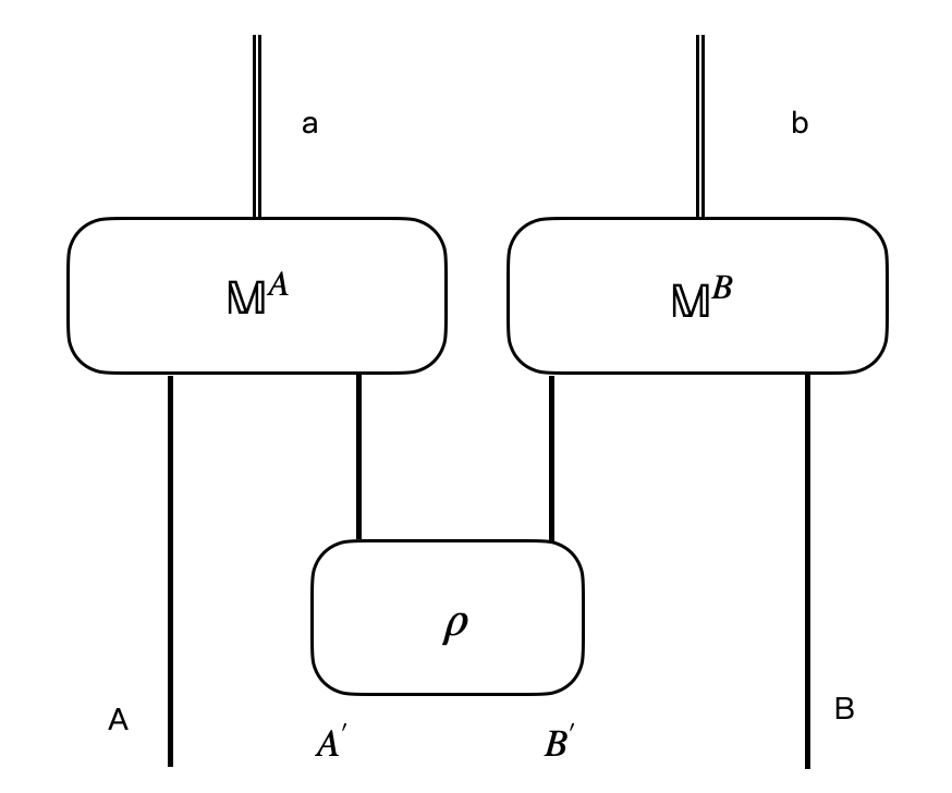
Figure 1: The schematic figure of a distributed measurement $\mathbb{M}^{AB}.$ It is composed of a bipartite mixed state $\rho$ and measurements $\mathbb{M}^{A}$ and $\mathbb{M}^{B}$ acting on Alice and Bob, respectively.

Assume $\mathbb{M}\in\mathcal{R}_{DM}$ is a distributed measurement, a straightforword problem is how to quantify $\mathbb{M}$ in this resource thoeory? Here we address the problem by proposing a quantifier through the robustness-based method.

Definition 1

Assume $\mathbb{M}=\{M_{ab}\}$ is a distributed measure, the quantifier based on the robustness method for this resource theory is defined as follows,

$$\mathrm{R}_{kDM}(\mathbb{M})= \min r$$ (5a)

s. t. $$M_{ab}\leq(1+r)O_{ab},$$ (5b)

$$\{O_{ab}\}\in\mathcal{F}_{kDM}\hskip 11.38109pt\forall a,b.$$ (5c)

In Sec. A.1, we present and prove the properties of $\mathrm{R}_{kDM}(\cdot)$, which can declare the validness of $\mathrm{R}_{kDM}(\cdot)$.

High Dimensional Teleportation Instruments. Quantum teleportation is one of the most fascinating and meaningful applications in quantum theory bennett1993teleporting . In the original quantum teleportation scheme, Alice and Bob share a maximally entangled state, and Charlie sends Alice an unknown state. Alice first performs a Bell-state measurement on the local bipartite systems; she then sends her shared state and the measurement result to Bob, who applies a unitary to his entangled state according to the received information. Finally, Bob obtains the state Alice received initially. Furthermore, the teleportation scheme can also be used to certify nonlocality. In 2017, the authors in cavalcanti2017all explored the non-classicality of teleportation schemes and presented a method to verify bipartite entanglement. The study in lipka2020 subsequently addressed the resource theory of the quantum teleportation scheme. First we introduce the concept of a quantum teleportation instrument.

Definition 2

Assume $\rho_{AB}$ is a bipartite mixed state, a teleportation instrument $\mathsf{\Lambda}=\{\Lambda_{i}|\mathcal{D}(\mathcal{H}_{A})\rightarrow\mathcal{D}(\mathcal{H}_{B})\}$ is a collection of subchannels

$$\Lambda_{i}(\varphi^{A})=\mathrm{tr}_{AA^{{}^{\prime}}}[(M_{i}^{AA^{{}^{\prime}}}\otimes\mathbb{I}^{B})(\varphi^{A}\otimes\rho^{A^{{}^{\prime}}B})].$$ (6)

Here $\mathbb{M}=\{M^{AA^{{}^{\prime}}}_{i}\}$ is a POVM.

Here we denote the set of all subchannels generated by $(\ref{c})$ as $\mathcal{R}_{sc}$. We say a teleportation instrument $\mathsf{\Lambda}$ is free when the Schmidt number of the shared state $\rho^{AB}$ which generates $\Lambda$ is less than $k,$ and the free set of teleportation instrument $\mathsf{\Lambda}$ is denoted as $\mathcal{F}_{sc}$. For a set of subchannels $\mathsf{\Lambda}$, we could quantify the resource under the robustness method,

$$1+\mathrm{R}_{sc}(\mathsf{\Lambda})= \hskip 14.22636pt1+r$$ (7)

s. t. $$\hskip 14.22636pt(1+r)\Gamma_{i}-{\Lambda}_{i}\geq_{pos}0,$$

$$\hskip 14.22636pt\mathsf{\Gamma}=\{\Gamma_{i}\}\in\mathcal{F}_{sc}.$$

Here $(1+r)\Gamma_{i}-{\Lambda}_{i}\geq_{pos}0$ means $(1+r)\Gamma_{i}-\Lambda_{i}$ is completely positive.

Remark 1

In Designolle2021genuine , the authors addressed the genuine high-dimensional quantum steering. They denote an assemblage $\{\sigma_{a|x}\}$ is $n$-preparable if $\sigma_{a|x}$ can be written as

$$\sigma^{B}_{a|x}=\mathrm{tr}_{A}[(A_{a|x}\otimes\mathbb{I})\rho^{AB}],$$

here $\rho^{AB}$ is a mixed state with $SN(\rho^{AB})=n$, and $A_{a|x}$ are semidefinite positive with $\sum_{a}A_{a|x}=\mathbb{I},$ $\forall x.$ Let $\Omega_{n}$ denote the set of all $n$-preparable assemblages. Due to the definition of $n$-preparable, there exists a hierarchical structure $\Omega_{n}\supset\Omega_{n-1}\supset\cdots\supset\Omega_{1}.$

In a teleportation instrument defined in Definition 2, assume this task is to let Bob obtain a set of states $\{\omega_{x}\}$ Alice initially received. In the process of the scheme, the set $\{\omega_{x}\}$ are inputted into the set of subchannels $\mathsf{\Lambda}=\{\Lambda_{i}\}$, and an enssemble $\{\tau^{B}_{i|x}\}$ is obtained, here

$$\tau_{i|x}=\mathrm{tr}_{AA^{{}^{\prime}}}[(M_{i}^{AA^{{}^{\prime}}}\otimes\mathbb{I}^{B})(\omega_{x}^{A}\otimes\rho^{A^{{}^{\prime}}B})].$$

As $SN(\omega_{x}^{A}\otimes\rho^{A^{{}^{\prime}}B})=SN(\rho^{A^{{}^{\prime}}B})$, the assemblage $\tau_{i|x}$ is $n$-preparable.

Relations between High Dimensional Distributed Measurements and Bipartite Mixed Entangled States. Assume $\rho^{A^{{}^{\prime}}B^{{}^{\prime}}}$ is a bipartite mixed state, we could generate distributed measurements and teleportation instrument with the aid of local measurements. One problem arises, what is the relation among the degrees of entanglement, the generated teleportation instruments and the generated distributed measurements quantitatively?

Theorem 1

Assume $\rho^{A^{{}^{\prime}}B^{{}^{\prime}}}$ is a bipartite state,

$$\mathrm{R}_{ke}(\rho^{A^{{}^{\prime}}B^{{}^{\prime}}})=\max_{\mathbb{M}^{A}}\mathrm{R}_{sc}(\mathsf{\Lambda}^{A\rightarrow B})=\max_{\mathbb{M}^{A},\mathbb{M}^{B}}\mathrm{R}_{kDM}(\mathbb{M}^{AB}).$$

where the maximum takes over all the local bipartite measurements $\mathbb{M}^{B}=\{M^{BB^{{}^{\prime}}}_{i}\}$ applied by Bob in the first equality, and the maximum takes over all the local bipartite measurements $\mathbb{M}^{A}=\{M^{AA^{{}^{\prime}}}_{i}\}$ and $\mathbb{M}^{B}=\{M^{BB^{{}^{\prime}}}_{i}\}$ operated by Alice and Bob in the second equality, respectively.

Here we place the proof of Theorem 1 in Sec. A.3

In the next section, we present a task of quantum state discrimination to show the advantages of high-dimensional entanglement.

Entanglement-assisted state discrimination. Assume Charles owns a bipartite state from the ensemble $\mathcal{G}=\{p_{xy},\sigma_{xy}\}$ according to the probability distribution $\{p_{xy}\}$, then according to the prior probability distribution, he sends one part of the state to Alice, while sends the other part of the state to Bob. Next Alice and Bob choose arbitrary local POVMs $\mathbb{M}^{A}=\{M_{a}^{AA^{{}^{\prime}}}\}$ and $\mathbb{M}^{B}=\{M_{b}^{BB^{{}^{\prime}}}\}$ to the states they received and their part of the state $\rho^{A^{{}^{\prime}}B^{{}^{\prime}}}$ and receive outcomes $a$ and $b$, respectively. At last, Alice and Bob win the game only if they both guess which state they received. Hence, the average probability of the game can be expressed as

$$p_{g}(\mathcal{G},\rho^{A^{{}^{\prime}}B^{{}^{\prime}}})=\max_{\mathbb{M}^{A},\mathbb{M^{B}}}\sum_{a,b,x,y}p_{xy}\mathrm{tr}(M_{ab}\sigma_{xy})\delta_{xa}\delta_{yb},$$

where the maximum takes over all the POVMs $\mathbb{M}^{A}$ of Alice and $\mathbb{M}^{B}$ of Bob with $M_{ab}$ ownning the form like (3). When restricting the shared state $\rho^{A^{{}^{\prime}}B^{{}^{\prime}}}$ in $\mathcal{F}_{sk}$, the best average probability of the above task is denoted as

$$p_{g}^{(k)}(\mathcal{G})=\max_{\delta^{A^{{}^{\prime}}B^{{}^{\prime}}}\in\mathcal{F}_{sk}}p_{g}(\mathcal{G},\delta^{A^{{}^{\prime}}B^{{}^{\prime}}}),$$

where the maximum takes over all the bipartite states with its Schmidt number less than $k.$

Theorem 2

Assume $\rho_{AB}$ is a bipartite state shared between Alice and Bob, let $\mathcal{G}=\{p_{xy},\sigma_{xy}\}$ be any ensemble of the bipartite states, then we have the following results,

$$\max_{\mathcal{G}}\frac{p_{g}(\mathcal{G},\rho^{A^{{}^{\prime}}B^{{}^{\prime}}})}{p_{g}^{(k)}(\mathcal{G})}=1+\mathrm{R}_{ke}(\rho^{A^{{}^{\prime}}B^{{}^{\prime}}}).$$

Here the maximum takes over all the ensembles $\mathcal{G}=\{p_{xy},\sigma_{xy}\}$ of bipartite states.

Here we place the proof of Theorem 2 in Sec. A.4.

Conclusions In this manuscript, we addressed the problem of certifying high-dimensional entanglement within the resource theories generated by the bipartite states considered here. First we introduced the resource theory of distributed measurement where the free objects are the distributed measurements generated by mixed states with Schmidt number less than $k$, then we presented the definition and properties of a quantifier for the resource by the robustness-based method. Next we presented the relation quantitatively among the high-dimensional entangled state, distributed measurements, and teleportation instruments. At last, we considered the task of entanglement-assisted state discrimination, and showed the advantages of high-dimensional entanglement, which can be quantified by the Schmidt-number robustness.

For the future work, it would be riveting to consider the corresponding resource theories in terms of multi-shot scenario for future work. Besides, it is intriguing to study the certifications on other high-dimensional objects under the quantum resource theories considered here.

Acknowledgement X. S. was supported by the National Natural Science Foundation of China (Grant No. 12301580).

Appendix A Supplemental Materials

In this section, we would first recall the knowledge needed of semidefinite programming (SDP), then we present the properties of $\mathrm{R}_{kDM}(\mathbb{M})$, next we consider the analytical expressions of $\mathrm{R}_{sc}(\Lambda)$ by a semidefinite programming. At last, we prove Theorem 1 and Theorem 2 in the main text.

Firstly, we recall the knowledge needed of SDP. Readers can refer to watrous2018theory ; gour2019comparison to learn more. Let $V_{1}$ and $V_{2}$ be two vector spaces, and let $K_{1}\subset V_{1}$ and $K_{2}\subset V_{2}$ be two convex cones. If $\Gamma:V_{1}\rightarrow V_{2}$ is a linear map, $H_{1}$ and $H_{2}$ are two given elements in $V_{1}$ and $V_{2}$, respectively,

The primal problem:

$$\alpha= \hskip 14.22636pt\min\mathrm{tr}(XH_{1})$$ (8)

s. t. $$\hskip 14.22636pt\Gamma(X)-H_{2}\in K_{2},$$

$$\hskip 14.22636ptX\in K_{1}.$$

The dual problem:

$$\beta= \hskip 14.22636pt\max\mathrm{tr}(YH_{2})$$ (9)

s. t. $$\hskip 14.22636ptH_{1}-\Gamma^{*}(Y)\in K_{1}^{*},$$

$$\hskip 14.22636ptY\in K^{*}_{2}.$$

Here $\Gamma^{*}:V_{2}\rightarrow V_{1}$ is the dual map of $\Gamma$, $K_{1}$ and $K_{2}$ are the dual cones of $K_{1}$ and $K_{2}$, respectively.

Next we present the strong duality conditions:

• Assume $K\subset V_{2}\oplus\mathbb{R}$ is a cone defined as

  $$K=\{(\Gamma(X)-Y,\mathrm{tr}XH_{1}):X\in K_{1},Y\in K_{2}\}.$$

  If $K$ is closed in $V_{2}\oplus\mathbb{R}$ and there exists a primal feasible plan, $\alpha=\beta.$

• The Slater’s condition: suppose that there is a primal feasible plan $X_{0}\in\emph{int}(K_{1})$ such that $\Gamma(X_{0})-H_{2}\in\emph{int}(K_{2})$. If there exists a primal optimal plan, then $\alpha=\beta.$

A.1 Properties of $\mathrm{R}_{kDM}(\mathbb{M})$

In this subsection, first we present the dual problem of $\mathrm{R}_{kDM}(\mathbb{M})$ for a POVM $\mathbb{M}$. Then we show the properties of $\mathrm{R}_{kDM}(\mathbb{M})$ defined in Theorem 3.

Here we first present the dual problem of $\mathrm{R}_{kDM}(\mathbb{M}).$ Assume $\mathbb{M}$ is a POVM, then $\mathrm{R}_{kDM}(\mathbb{M})$ can be written as follows,

$$1+\mathrm{R}_{kDM}(\mathbb{M})=\hskip 14.22636pt \min\frac{1}{d^{2}}\mathrm{tr}\sum_{ab}\tilde{O}_{ab}$$ (10)

s. t. $$M_{ab}\leq\tilde{O}_{ab},$$

$$\{\tilde{O}_{ab}\}\in\tilde{\mathcal{F}}_{kDM}\hskip 11.38109pt\forall a,b.$$

Here $\tilde{O}_{ab}=(1+r)O_{ab},$ and $\tilde{\mathcal{F}}_{kDM}$ is the cone of $\mathcal{F}_{kDM}.$ As $\mathbb{O}$ is a POVM,

$$\sum_{ab}O_{ab}=\mathbb{I}_{AB},\hskip 14.22636pt\mathrm{tr}\sum_{ab}O_{ab}=d^{2},$$

here $dim(\mathcal{H}_{A})=dim(\mathcal{H}_{B})=d.$ The duality problem of (10) is

$$1+\mathrm{R}_{kDM}(\mathbb{M})=\hskip 14.22636pt \frac{1}{d^{2}}\max\sum_{ab}Y_{ab}M_{ab}$$ (11)

s. t. $$\mathbb{I}-Y_{ab}\in\tilde{\mathcal{F}}_{kDM}^{*},$$

$$Y_{ab}\geq 0.$$ (12)

Moreover, (10) can also be written as follows,

$$1+\mathrm{R}_{kDM}(\mathbb{M})=\hskip 14.22636pt 1+\min r$$ (13)

s. t. $$M_{ab}\leq\tilde{O}_{ab}$$

$$\sum_{a,b}\tilde{O}_{ab}=(1+r)\mathbb{I}^{AB}$$

$$\tilde{\mathbb{O}}\in\tilde{\mathcal{F}}_{kDM}.$$

Then we present the duality problem of (13),

$$1+\mathrm{R}_{kDM}(\mathbb{M})= \hskip 14.22636pt\max\sum_{a,b}\mathrm{tr}(Y_{ab}M_{ab})$$

s. t. $$\hskip 14.22636ptK-Y_{ab}\in\tilde{\mathcal{F}}_{kDM}^{*},$$

$$\hskip 14.22636pt\mathrm{tr}K=1,\hskip 11.38109ptY_{ab}\geq 0.$$ (14)

Here $\tilde{\mathcal{F}}^{*}_{kDM}=\{Z|\mathrm{tr}(XZ)\geq 0,X\in\tilde{\mathcal{F}}_{kDM}\}$.

Next we would recall the definition of simulability of distributed measurements, first we introduce the definition of $n$-partially entanglement breaking ($n$-PEB).

Definition 3

Chruscinski2006on A channel $\Lambda$ is $n$-PEB if $SN(\Lambda\otimes\mathbb{I}(\rho^{AB}))\leq n$ for all bipartite states $\rho^{AB}.$

The definition of simulability of distributed measurements in the resource theory considered here is based on $n$-PEB.

Definition 4

Assume $\mathbb{M}^{AB}=\{M^{AB}_{ij}\}$ and $\mathbb{N}^{AB}=\{N^{AB}_{mn}\}$ are two distributed POVMs, we say $\mathbb{N}^{AB}$ can be simulated by $\mathbb{M}^{AB}$, if

$$N^{AB}_{mn}=\sum_{ij\lambda}p_{\lambda}p(m,n|i,j,\lambda)\mathcal{E}_{\lambda}^{\dagger}[M^{AB}_{ij}],$$ (15)

here $p_{\lambda}$ is a probability distribution, $\mathcal{E}_{\lambda}$ is $n$-PEB. When a POVM $\mathbb{N}$ can be simulated by a POVM $\mathbb{M}$ under the way defined in (15), we denote $\mathbb{N}\preceq\mathbb{M}.$

Theorem 3

Assume $\mathbb{M}^{AB}\in\mathcal{R}_{kDM}$ is a distributed measurement, the quantifier $\mathrm{R}_{kDM}(\mathbb{M})$ defined in Definition 1 satifies the following properties,

• [Faithfulness] $\mathrm{R}_{kDM}(\mathbb{M})$ vanishes if and only if the measurement $\mathbb{M}$ is free.

  $$\mathrm{R}_{kDM}(\mathbb{M})=0\hskip 14.22636pt\Longleftrightarrow\hskip 14.22636pt\mathbb{M}\in\mathcal{F}_{kDM}.$$

• [Convexity] Assume $\mathbb{M}_{1}$ and $\mathbb{M}_{2}$ are two distributed measurements in $\mathcal{R}_{DM},$ let $\mathbb{M}=p\mathbb{M}_{1}+(1-p)\mathbb{M}_{2}$,

  $$\mathrm{R}_{kDM}(\mathbb{M})\leq p\mathrm{R}_{kDM}(\mathbb{M}_{1})+(1-p)\mathrm{R}_{kDM}(\mathbb{M}_{2}),$$

  here $p\in(0,1).$

• [Monotonicity] Assume $\mathbb{N}$ and $\mathbb{M}$ are two distributed measurement, if $\mathbb{N}$ can be simulated by $\mathbb{M}$ under the simulation strategy defined by (15), $i.$ $e.$ $\mathbb{N}\preceq\mathbb{M},$ then

  $$\mathrm{R}_{kDM}(\mathbb{N}^{AB})\leq\mathrm{R}_{kDM}(\mathbb{M}^{AB}).$$

Proof of Theorem 3:

• [Faithfulness] $\Longrightarrow:$ If $\mathbb{M}\in\mathcal{F}_{kDM}$, then we can choose $r=0$ in (5a), as $\mathrm{R}_{kDM}(\cdot)$ is nonnegative, $r=0$ is optimal.

  $\Longleftarrow:$ Due to the definition of $\mathrm{R}_{kDM}(\cdot)$, it is straightword to obtain that $\mathbb{M}\in\mathcal{F}_{kDM}$.

• [Convexity] Assume $\tilde{\mathbb{O}}_{1}$ and $\tilde{\mathbb{O}}_{2}$ are two optimal POVMs in $\tilde{\mathcal{F}}_{kDM}$ in terms of $\mathrm{R}_{kDM}(\cdot)$ for $\mathbb{M}_{1}$ and $\mathbb{M}_{2}$, respectively. As the set of bipartite states with Schmidt number less than $k$ is convex, $p\tilde{\mathbb{O}}_{1}+(1-p)\tilde{\mathbb{O}}_{2}\in\mathcal{F}_{kDM}.$ As

  $$1+\mathrm{R}_{kDM}(\mathbb{M}^{{}^{\prime}})$$

  $$\leq \frac{1}{d_{A}d_{B}}[p\mathrm{tr}(\sum_{ab}\tilde{O}_{ab}^{1})+(1-p)\mathrm{tr}(\sum_{ab}\tilde{O}_{ab}^{2})]$$

  $$= p\mathrm{R}_{kDM}(\mathbb{M}_{1})+(1-p)\mathrm{R}_{kDM}(\mathbb{M}_{2})+1.$$

• [Monotonicity] As $\mathbb{N}\preceq\mathbb{M},$ there exist a probability distribution $\{p_{\lambda}\}$ and $n$-PEB $\{\mathcal{E}_{\lambda}\}$ such that

  $$N_{mn}=\sum_{ij\lambda}p_{\lambda}p(m,n|i,j,\lambda)\mathcal{E}_{\lambda}^{\dagger}[M_{ij}].$$

  Next assume $\mathbb{Y}=\{Y_{mn}\}$ and $K$ are the optimal for $\mathbb{N}$ in terms of the definition of $\mathrm{R}_{B}(\cdot)$, let $Z_{ij}=\sum p_{\lambda}p(a,b|i,j,\lambda)\mathcal{E}_{\lambda}[Y_{ab}]$. Let $\mathbb{H}=\{H_{mn}\}$ and $K$ be arbitrary in $\tilde{\mathcal{F}}_{kDM}$ and $\mathcal{F}_{sk}$, respectively, then

  $$\mathrm{tr}[H_{mn}(K-\sum_{i,j,\lambda}p_{\lambda}p(m,n|i,j,\lambda)\mathcal{E}_{\lambda}[Y_{mn}])]$$

  $$= \mathrm{tr}[H_{mn}(\sum_{\lambda}\mathcal{E}_{\lambda}(K-\sum_{m,n}p_{\lambda}p(m,n|i,j,\lambda)Y_{mn}))]$$

  $$\geq \mathrm{tr}[H_{mn}(\sum_{\lambda}\mathcal{E}_{\lambda}\sum_{m,n}p_{\lambda}p(m,n|i,j,\lambda)(K-Y_{mn}))]$$

  $$\geq 0$$

  Here the first equality is due to that $\sum_{\lambda}\mathcal{E}_{\lambda}$ is a channel, and $\mathrm{tr}\sum_{\lambda}\mathcal{E}_{\lambda}(K)=\mathrm{tr}K.$ By the definition of $Y_{mn}$ and $(\ref{r4})$, the last inequality is valid. That is, $\mathbb{Z}=\{Z_{ab}\}$ satisfies the conditions of the dual problem (14). Hence,

  $$\mathrm{R}_{kDM}(\mathbb{M})\geq \sum_{i,j}\mathrm{tr}(Z_{ij}M_{ij})$$

  $$= \sum_{i,j}\mathrm{tr}(\sum p_{\lambda}p(a,b|i,j,\lambda)\mathcal{E}_{\lambda}[Y_{ab}]M_{ij})$$

  $$= \sum_{a,b}\mathrm{tr}(\sum_{ij\lambda}p_{\lambda}p(a,b|i,j,\lambda)Y_{ab}\mathcal{E}_{\lambda}^{\dagger}(M_{ij}))$$

  $$= \sum_{i,j}\mathrm{tr}(Y_{ij}N_{ij})$$

  $$= \mathrm{R}_{kDM}(\mathbb{N}).$$

  Then we finish the proof.

A.2 Properties of $\mathrm{R}_{sc}(\mathsf{\Lambda})$.

In this part, before presenting the properties of $\mathrm{R}_{sc}(\mathsf{\Lambda})$, we would restate $\mathrm{R}_{sc}(\cdot)$. Assume $\{M_{a}^{AA^{{}^{\prime}}}\}$ is a POVM, $\rho_{A^{{}^{\prime}}B}$ is a state shared by Alice and Bob. Next we let $J_{a}$ denotes the Choi-Jamiolkowski isomorphism of $\Lambda_{a}$, that is, $J_{a}=(\mathbb{I}\otimes\Lambda_{a})[|\psi_{+}\rangle\langle\psi_{+}|]$, here $|\psi_{+}\rangle=\frac{1}{\sqrt{d}}\sum_{i=1}^{d}|ii\rangle$ is the maximally entangled state. Hence, $\mathrm{R}_{sc}(\Lambda)$ can be written as

$$1+\mathrm{R}_{sc}(\mathsf{\Lambda})= \hskip 14.22636pt\min\mathrm{tr}\tilde{\sigma}^{B^{{}^{\prime}}}$$ (16)

s. t. $$\hskip 14.22636ptJ_{a}^{VB^{{}^{\prime}}}\leq O_{a}^{VB^{{}^{\prime}}}\hskip 8.53581pt\forall a,$$

$$\hskip 14.22636pt\sum_{a}O_{a}^{VB^{{}^{\prime}}}=\frac{\mathbb{I}}{d}\otimes\tilde{\sigma}^{B^{{}^{\prime}}},$$

$$\hskip 14.22636ptO_{a}^{VB^{{}^{\prime}}}\in\mathcal{F}_{sk}.\hskip 8.53581pt\forall a,$$

$$\hskip 14.22636pt\tilde{\sigma}^{B^{{}^{\prime}}}\geq 0.$$

Then the dual problem of $\mathrm{R}_{sc}(\mathsf{\Lambda})$ can be written as

$$1+\mathrm{R}_{sc}(\mathsf{\Lambda})= \hskip 14.22636pt\max\sum_{a}\mathrm{tr}(Y_{a}J_{a})$$ (17)

s. t. $$\hskip 14.22636ptM-Y_{a}\in\mathcal{F}_{sk}^{*},$$

$$\hskip 14.22636pt\mathrm{tr}_{V}M=\mathbb{I},$$

$$\hskip 14.22636ptY_{a}\geq 0.$$

Next we show that $\mathrm{R}_{sc}(\cdot)$ satisfies the following properties:

• [Faithfulness]$\Longleftarrow:$ If $\mathrm{R}_{sc}(\mathsf{\Lambda})=0$, then due to the definition of $\mathrm{R}_{kDM}(\cdot)$, we have $\mathsf{\Lambda}\in\mathcal{F}_{sc}.$

  $\Longrightarrow:$ If $\mathsf{\Lambda}\in\mathcal{F}_{sc},$ when taking $\Gamma_{i}$ in (7) as $\Lambda_{i}$, $r=0$. As $r$ is nonnegative, $r=0$ is the minimum.

• [Convexity] Assume $\mathsf{\Lambda}_{1}=\{\Lambda_{a}^{(1)}\}$ and $\mathsf{\Lambda}_{2}=\{\Lambda_{a}^{(2)}\}$ are two sets of subchannels generated under the Definition 2, $\{O_{a}\}$ and $\{Q_{a}\}$ are the optimal for $\mathsf{\Lambda}_{1}$ and $\mathsf{\Lambda}_{2}$ in terms of (16), respectively, then based on $\mathrm{R}_{sc}(\mathsf{\Lambda})$ defined in (16), $\mathrm{R}_{sc}(\mathsf{\Lambda}_{1})=\sum_{a}\mathrm{tr}(O_{a}),$ $\mathrm{R}_{sc}(\mathsf{\Lambda}_{2})=\sum_{a}\mathrm{tr}(Q_{a})$. Let $J_{a}$ and $K_{a}$ be the Choi-Jamiolkowski isomorphism of $\Lambda^{(1)}_{a}$ and $\Lambda^{(2)}_{a},$ respectively. Let $\mathsf{\Gamma}=p\mathsf{\Lambda}_{1}+(1-p)\mathsf{\Lambda}_{2},$ $p\in(0,1),$ $pJ_{a}+(1-p)K_{a}$ are Choi-Jamiolkowski isomorphism of subchannels in $\mathsf{\Gamma},$

  $$1+\mathrm{R}_{sc}(\Gamma)\leq p\sum_{a}\mathrm{tr}(O_{a})+(1-p)\mathrm{tr}(Q_{a})$$

  $$= p[1+\mathrm{R}_{sc}(\mathsf{\Lambda_{1}})]+(1-p)[1+\mathrm{R}_{sc}(\mathsf{\Lambda_{2}})].$$

  The first inequality is due to that $pO_{a}+(1-p)Q_{a}\geq pJ_{a}+(1-p)K_{a}$. Hence, we finish the proof of $\mathrm{R}_{sc}(\Gamma)\leq p\mathrm{R}_{sc}(\Lambda_{1})+(1-p)\mathrm{R}_{sc}(\Lambda_{1}).$

A.3 Proof of Theorem 1

In this subsection, we mainly present the proof of Theorem 1. Before proving Theorem 1, we first present the dual problem of $\mathrm{R}_{e}(\cdot)$, then we get some Lemmas needed to show Theorem 1.

Based on the knowledge of semidefinite programming given in Sec. A.1, we present the dual problem of $\mathrm{R}_{ke}(\rho_{AB})$,

$$1+\mathrm{R}_{ke}(\rho_{AB})=\hskip 14.22636pt \max\mathrm{tr}(A\rho)$$

s. t. $$\mathbb{I}-A\in\mathcal{F}_{sk}^{*},$$

$$\hskip 14.22636ptA\geq 0.$$ (18)

Lemma 4

Let $\rho^{A^{{}^{\prime}}B}$ be a bipartite mixed state, assume $\mathbb{M}^{A}=\{M_{a}^{AA^{{}^{\prime}}}\}_{a}$ is an arbitrary POVM operated by Alice, $\mathsf{\Lambda}=\{\Lambda_{i}\}$ is a set of subchannels defined in (6) generated by $\mathbb{M}^{A}$ and $\rho^{A^{{}^{\prime}}B}$, then

$$\mathrm{R}_{ke}(\rho)=\max_{\mathbb{M}^{A}}\mathrm{R}_{sc}(\mathsf{\Lambda}),$$

where the maximum takes over all the POVMs $\mathbb{M}^{A}.$

Proof: First we show that $r_{1}=\mathrm{R}_{ke}(\rho)\geq\mathrm{R}_{sc}(\Lambda).$ Let $\gamma_{A^{{}^{\prime}}B}$ be the optimal for $\rho^{A^{{}^{\prime}}B}$ in terms of $\mathrm{R}_{ke}(\rho_{A^{{}^{\prime}}B})$, and let $\mathsf{\Gamma}=\{\Gamma_{i}(\cdot)\}$ be the set of subchannels such that

$$\Gamma_{i}(\phi^{A})=\mathrm{tr}_{AA^{{}^{\prime}}}[(M_{i}^{AA^{{}^{\prime}}}\otimes\mathbb{I}^{B})(\phi^{A}\otimes\gamma^{A^{{}^{\prime}}B})],$$

then we have

$$(1+r_{1})\Gamma_{i}-\Lambda_{i}\in\mathcal{R}_{sc}.$$

As $\gamma_{A^{{}^{\prime}}B}$ is a state with $SN(\gamma)\leq k,$ then $\mathsf{\Gamma}\in\mathcal{F}_{sc}.$ Due to the definition of $\mathrm{R}_{sc}(\Lambda)$, $\mathrm{R}_{ke}(\rho)\geq\mathrm{R}_{sc}(\Lambda).$

Next we present a teleportation instrument $\mathsf{\Lambda}$ such that $\mathrm{R}_{ke}(\rho)\leq\mathrm{R}_{sc}(\Lambda).$ Assume $\{U_{i}\}$ is a set of Pauli operators with respect to the basis $\{|i\rangle^{V}\},$ let $A$ be the optimal for $\rho^{A^{{}^{\prime}}B^{{}^{\prime}}}$ in terms of $\mathrm{R}_{ke}(\rho^{A^{{}^{\prime}}B})$. Let

$$Y^{VB}_{a}= \frac{1}{d}(\mathcal{U}^{V}_{a}\otimes\mathbb{I})(A^{VB})^{T},$$

$$M^{VA^{{}^{\prime}}}_{a}= (\mathcal{U}^{V}_{a}\otimes\mathbb{I})(\psi_{+}),$$

here $\mathcal{U}_{a}(\cdot)=U_{a}(\cdot)U_{a}^{\dagger}$, then

$$1+\max_{\mathbb{M}^{A}}\mathrm{R}_{sc}(\mathsf{\Lambda})\geq \sum_{a}\mathrm{tr}Y_{a}J_{a}$$

$$= \sum_{a}\mathrm{tr}[(Y_{a}^{VB}\otimes\mathbb{I}^{AA^{{}^{\prime}}})(M_{a}^{AA^{{}^{\prime}}}\otimes\mathbb{I}^{VB})(\psi_{+}^{VA}\otimes\rho^{A^{{}^{\prime}}B})]$$

$$= \sum_{a}\mathrm{tr}[(Y_{a}^{VB}\otimes\mathbb{I}^{AA^{{}^{\prime}}})((M_{a}^{VA^{{}^{\prime}}})^{T}\otimes\mathbb{I}^{VB})(\psi_{+}^{VA}\otimes\rho^{A^{{}^{\prime}}B})]$$

$$= \frac{1}{d}\sum_{a}\mathrm{tr}[(Y_{a}^{VB}\otimes\mathbb{I}^{A^{{}^{\prime}}})((M_{a}^{VA^{{}^{\prime}}})^{T}\otimes\mathbb{I}^{B})(\mathbb{I}^{A}\otimes\rho^{A^{{}^{\prime}}B})]$$

$$= \frac{1}{d^{2}}\sum_{a}\mathrm{tr}_{VA^{{}^{\prime}}B}[(\mathcal{U}^{V}_{a}\otimes\mathbb{I})(A^{VB})^{T}\otimes\mathbb{I}^{A^{{}^{\prime}}}][(\mathcal{U}^{V}_{a}\otimes\mathbb{I})(\psi_{+})](\mathbb{I}^{V}\otimes\rho^{A^{{}^{\prime}}B})]$$

$$= \mathrm{tr}(A\rho)$$

$$= 1+\mathrm{R}_{ke}(\rho^{A^{{}^{\prime}}B}).$$

Hence, we finish the proof.

Lemma 5

Assume $\rho^{AB}$ is a bipartite mixed state, $\mathbb{M}^{A}=\{M_{i}^{AA^{{}^{\prime}}}\}_{i}$ is a POVM, $\mathsf{\Lambda}=\{\Lambda_{i}\}_{i}$ is a set of subchannels defined in (6), then

$$\mathrm{R}_{sc}(\mathsf{\Lambda})=\max_{\mathbb{M}^{B}}(\mathbb{M}^{AB}),$$

where $\mathbb{M}^{AB}$ is defined in (3), and the maximum takes over all the POVMs $\mathbb{M}^{B}=\{M^{BB^{{}^{\prime}}}\}.$

Proof: First we show that $\mathrm{R}_{sc}(\mathsf{\Lambda})$ is lower than $\max_{\mathbb{M}^{B}}(\mathbb{M}^{AB}).$

Let $\{Y_{a}\}$ and $M$ be the optimal for $\mathsf{\Lambda}$ in terms of (17), let $\{U_{b}^{B}\}$ be a set of Pauli operators with respect to the basis $\{|i\rangle_{B}\}$. Let

$$M_{b}^{BB^{{}^{\prime}}}= (\mathcal{U}_{b}\otimes\mathbb{I})(\psi_{+}^{{BB^{{}^{\prime}}}})$$

$$A_{ab}= (\mathcal{U}_{b}\otimes\mathbb{I})(Y_{a}^{T}),$$

$$K= \frac{1}{d}(\mathcal{U}_{b}\otimes\mathbb{I})(M^{T}),$$

here $\mathcal{U}_{b}(\cdot)=U_{b}(\cdot)U_{b}^{\dagger}$.

Based on the definitions of $\{Y_{a}\}$ and $M$, $\{A_{ab}\}$ and $K$ satisfy the restricted conditions in $(\ref{r4})$, hence we have

$$1+\max_{\mathbb{M}^{B}}\mathrm{R}_{B}(\mathbb{M}^{AB})$$ (19)

$$\geq \sum_{ab}\mathrm{tr}(A_{ab}M_{ab})$$

$$= \sum_{ab}\mathrm{tr}[(\mathcal{U}_{b}\otimes\mathbb{I})(Y_{a}^{T})\otimes\mathbb{I}_{A^{{}^{\prime}}B^{{}^{\prime}}}][(M^{AA^{{}^{\prime}}}_{a}\otimes(\mathcal{U}_{b}\otimes\mathbb{I})(\psi_{+}^{BB^{{}^{\prime}}}))(\mathbb{I}^{A}\otimes\rho_{A^{{}^{\prime}}B^{{}^{\prime}}}\otimes\mathbb{I}^{B})]$$

$$= \frac{1}{d^{2}}\sum_{ab}\mathrm{tr}[Y_{a}^{AB^{{}^{\prime}}}(M_{a}^{AA^{{}^{\prime}}}\otimes\mathbb{I}^{BB^{{}^{\prime}}})(\psi_{+}^{VA}\otimes\rho^{A^{{}^{\prime}}B^{{}^{\prime}}})]$$ (20)

$$= \sum_{a}\mathrm{tr}[Y_{a}J_{a}]$$

$$= 1+\mathrm{R}_{sc}(\mathsf{\Lambda}).$$ (21)

Then we show the inequality of the other side. Assume $\mathbb{M}^{AB}=\{M_{ab}^{AB}\}$ is generated under the fomula (3), then we could construct $\mathbb{N}^{VB}=\{N_{ab}\}$ such that

$$N_{ab}^{VB}=d\mathrm{tr}_{A}[(\mathbb{I}^{V}\otimes M_{ab}^{AB})(\psi_{+}^{VA}\otimes\mathbb{I}^{B})],$$

here $\psi_{+}^{VA}$ is the maximally entangled state. As $(\mathbb{I}\otimes A)|\psi\rangle=(A^{T}\otimes\mathbb{I})|\psi\rangle$, $N_{ab}^{T}=M_{ab}$.

$$N_{ab}^{VB}$$ (22)

$$= d\mathrm{tr}_{AA^{{}^{\prime}}B^{{}^{\prime}}}[(\mathbb{I}^{V}\otimes M_{a}^{AA^{{}^{\prime}}}\otimes M^{BB^{{}^{\prime}}}_{b})(\psi_{+}^{VA}\otimes\rho^{A^{{}^{\prime}}B^{{}^{\prime}}}\otimes\mathbb{I}^{B})]$$ (23)

$$= \mathrm{tr}_{B^{{}^{\prime}}}[(\mathbb{I}^{V}\otimes M_{b}^{BB^{{}^{\prime}}})(J_{a}^{VB^{{}^{\prime}}}\otimes\mathbb{I}^{B})],$$ (24)

the second equality is due to the definition of $\Lambda_{i}(\cdot)$ defined in Definition 2, the Choi-Jamiolkowski isomorphism of subchannels $\Lambda_{a}$, and $(\mathbb{I}\otimes A)|\psi\rangle=(A^{T}\otimes\mathbb{I})|\psi\rangle$. Due to the definition of $\mathrm{R}_{sc}(\mathsf{\Lambda})$, we have

$$J_{a}^{VB^{{}^{\prime}}}\leq[1+\mathrm{R}_{sc}(\mathsf{\Lambda})]O_{a},\hskip 8.53581pt\{O_{a}\}\in\mathcal{F}_{sk},$$

combing the above formula, (24) can be turned into

$$N_{ab}^{VB}\leq [1+\mathrm{R}_{sc}(\mathsf{\Lambda})]\mathrm{tr}_{B^{{}^{\prime}}}[(\mathbb{I}^{V}\otimes M_{b}^{BB^{{}^{\prime}}})(O_{a}^{VB^{{}^{\prime}}}\otimes\mathbb{I}^{B})]$$

$$= [1+\mathrm{R}_{sc}(\mathsf{\Lambda})]T_{ab},$$

here $\{T_{ab}\}$ is in $\mathcal{F}_{B}.$ Then we have

$$N^{AB}_{ab}\leq[1+\mathrm{R}_{sc}(\mathsf{\Lambda})]T_{ab}^{AB}.$$

Hence, due to the definition of $\mathrm{R}_{kDM}(\mathbb{M}^{AB})$, and the set $\mathcal{F}_{kDM}$ is closed under the transpose $(\cdot)^{T}$, we have $\max_{\mathbb{M}^{B}}\mathrm{R}_{kDM}(\mathbb{M}^{AB})\leq\mathrm{R}(\mathsf{\Lambda})$.

At last, by combing (21), we have $\max_{\mathbb{M}^{B}}\mathrm{R}_{kDM}(\mathbb{M}^{AB})\leq\mathrm{R}(\mathsf{\Lambda}).$ At last, we show $\max_{\mathbb{M}^{B}}\mathrm{R}_{kDM}(\mathbb{M}^{AB})=\mathrm{R}(\mathsf{\Lambda}).$

Proof of Theorem 1: First we prove $\mathrm{R}_{ke}(\rho_{AB})\geq\mathrm{R}_{kDM}(\mathbb{M}).$ Assume $\mathrm{R}_{ke}(\rho_{AB})=r,$ $\sigma_{AB}$ and $\gamma_{AB}$ are the states defined in (2) for $\mathrm{R}_{ke}(\rho_{AB})$, then let

$$M^{{}^{\prime}}_{ab}= \mathrm{tr}_{A^{{}^{\prime}}B^{{}^{\prime}}}[(M_{a}^{AA^{{}^{\prime}}}\otimes M_{b}^{BB^{{}^{\prime}}})(\mathbb{I}_{A}\otimes\sigma_{A^{{}^{\prime}}B^{{}^{\prime}}}\otimes\mathbb{I}_{B})],$$

$$M_{ab}^{{}^{\prime\prime}}= \mathrm{tr}_{A^{{}^{\prime}}B^{{}^{\prime}}}[(M_{a}^{AA^{{}^{\prime}}}\otimes M_{b}^{BB^{{}^{\prime}}})(\mathbb{I}_{A}\otimes\gamma_{A^{{}^{\prime}}B^{{}^{\prime}}}\otimes\mathbb{I}_{B})].$$

Due to the above definition, we have $\{M_{ab}^{{}^{\prime\prime}}\}\in\mathcal{F}_{kDM},$ and $M_{ab}\leq(1+r)O_{ab}$. By the definition of $\mathrm{R}_{kDM}(\cdot),$ we finish the proof of $\mathrm{R}_{e}(\rho_{AB})\geq\mathrm{R}_{kDM}(\mathbb{M}).$

At last, we show the other side of the inequality. By Lemma 5, we have

$$\max_{\mathbb{M}^{A},\mathbb{M}^{B}}\mathrm{R}_{kDM}(\mathbb{M}^{AB})=\max_{\mathbb{M}^{A}}[\max_{\mathbb{M}^{B}}\mathrm{R}_{kDM}(\mathbb{M}^{AB})]=\max_{\mathbb{M}^{A}}\mathrm{R}(\mathsf{\Lambda}^{A\rightarrow B^{{}^{\prime}}}).$$

That is, if we prove $\max_{\mathbb{M}^{A}}\mathrm{R}(\mathsf{\Lambda}^{A\rightarrow B^{{}^{\prime}}})\geq\mathrm{R}_{e}(\rho_{AB})$, we finish the proof.

Assume $A$ is the optimal for $\rho$ in terms of $\mathrm{R}_{ke}(\cdot)$. Let $\{U_{a}\}_{a=1}^{d^{{}^{\prime}}}$ be a set of Pauli operators with respect to $\{|i\rangle^{A^{{}^{\prime}}}\}$. Let $\mathbb{M}^{A}=\{M_{a}^{AA^{{}^{\prime}}}=(\mathbb{I}\otimes\mathcal{U}_{a})[\psi_{+}]\}$. Based on the above assumption, let $M$, $Y_{a}$ and $\mathbb{M}^{A}$ be the following

$$M=\frac{1}{d}\mathbb{I},\hskip 8.53581ptY_{a}=(\mathbb{I}\otimes\mathcal{U}_{a})[A],\hskip 11.38109ptM_{a}^{AA^{{}^{\prime}}}=(\mathbb{I}\otimes\mathcal{U}_{a})(\psi_{+}),$$

which are appropriate for $\mathrm{R}_{sc}(\mathsf{\Lambda})$ in terms of (17).

Hence, we have

$$1+\max_{\mathbb{M}^{A}}\mathrm{R}(\mathsf{\Lambda}^{A\rightarrow B^{{}^{\prime}}})$$

$$\geq \sum_{a}\mathrm{tr}(Y_{a}J_{a})$$

$$= \sum_{a}\mathrm{tr}[(\mathbb{I}\otimes\mathcal{U}_{a}[A])\mathrm{tr}_{AA^{{}^{\prime}}}[(\mathbb{I}^{V}\otimes M_{a}^{AA^{{}^{\prime}}}\otimes\mathbb{I}^{B^{{}^{\prime}}})(\psi_{+}\otimes\rho)]]$$

$$= \sum_{a}\mathrm{tr}[(\mathbb{I}\otimes\mathcal{U}_{a}[A])\otimes\mathbb{I}_{AA^{{}^{\prime}}}][(\mathbb{I}^{V}\otimes(\mathbb{I}\otimes\mathcal{U}_{a})(\psi_{+})\otimes\mathbb{I}^{B^{{}^{\prime}}})(\psi_{+}\otimes\rho)]$$

$$= \mathrm{tr}(A\rho)$$

$$= 1+\mathrm{R}_{ke}(\rho).$$

Then we finish the proof of this theorem.

A.4 Proof of Theorem 2

In the proof, let $\mathrm{R}_{ke}(\rho)=r,$ and $\gamma$ is the optimal in terms of $\mathrm{R}_{ke}(\cdot)$ for $\rho$,

$$\rho_{AB}\leq(1+r)\gamma_{AB},\hskip 11.38109ptSN(\gamma_{AB})\leq k.$$

Then

$$p_{g}(\mathcal{G},\rho_{AB})= \max_{\mathbb{M}^{A},\mathbb{M^{B}}}\sum_{a,b,x,y}p_{xy}\mathrm{tr}(M_{ab}\sigma_{xy})$$

$$= \max_{\mathbb{M}^{A},\mathbb{M^{B}}}\sum_{a,b,x,y}p_{xy}\mathrm{tr}(M_{x}^{AA^{{}^{\prime}}}\otimes M_{y}^{BB^{{}^{\prime}}})(\rho^{AB}\otimes\mathbb{I}^{A^{{}^{\prime}}B^{{}^{\prime}}})(\mathbb{I}^{AB}\otimes\sigma^{A^{{}^{\prime}}B^{{}^{\prime}}}_{xy})$$

$$\leq (1+r)\max_{\mathbb{M}^{A},\mathbb{M^{B}}}\sum_{a,b,x,y}p_{xy}\mathrm{tr}(M_{x}^{AA^{{}^{\prime}}}\otimes M_{y}^{BB^{{}^{\prime}}})(\gamma^{AB}\otimes\mathbb{I}^{A^{{}^{\prime}}B^{{}^{\prime}}})(\mathbb{I}^{AB}\otimes\sigma^{A^{{}^{\prime}}B^{{}^{\prime}}}_{xy}),$$

$$\frac{p_{g}(\mathcal{G},\rho_{AB})}{p_{g}^{(k)}(\mathcal{G})}= \frac{\sum_{a,b,x,y}p_{xy}\mathrm{tr}(M_{x}^{AA^{{}^{\prime}}}\otimes M_{y}^{BB^{{}^{\prime}}})(\rho^{AB}\otimes\mathbb{I}^{A^{{}^{\prime}}B^{{}^{\prime}}})(\mathbb{I}^{AB}\otimes\sigma^{A^{{}^{\prime}}B^{{}^{\prime}}}_{xy})}{\max_{\delta\in\mathcal{F}_{sk}}\sum_{a,b,x,y}p_{xy}\mathrm{tr}(M_{x}^{AA^{{}^{\prime}}}\otimes M_{y}^{BB^{{}^{\prime}}})(\delta^{AB}\otimes\mathbb{I}^{A^{{}^{\prime}}B^{{}^{\prime}}})(\mathbb{I}^{AB}\otimes\sigma^{A^{{}^{\prime}}B^{{}^{\prime}}}_{xy})}$$

$$\leq \frac{(1+r)\sum_{a,b,x,y}p_{xy}\mathrm{tr}(M_{x}^{AA^{{}^{\prime}}}\otimes M_{y}^{BB^{{}^{\prime}}})(\delta^{AB}\otimes\mathbb{I}^{A^{{}^{\prime}}B^{{}^{\prime}}})(\mathbb{I}^{AB}\otimes\sigma^{A^{{}^{\prime}}B^{{}^{\prime}}}_{xy})}{\max_{\delta\in\mathcal{F}_{sk}}\sum_{a,b,x,y}p_{xy}\mathrm{tr}(M_{x}^{AA^{{}^{\prime}}}\otimes M_{y}^{BB^{{}^{\prime}}})(\delta^{AB}\otimes\mathbb{I}^{A^{{}^{\prime}}B^{{}^{\prime}}})(\mathbb{I}^{AB}\otimes\sigma^{A^{{}^{\prime}}B^{{}^{\prime}}}_{xy})}$$

$$\leq 1+r.$$

The first inequality is due to that $\delta$ is the optimal in terms of $\mathrm{R}_{ke}(\cdot)$ for $\rho$. Hence, we have

$$\max_{\mathcal{G}}\frac{p_{g}(\mathcal{G},\rho_{AB})}{p_{g}^{(k)}(\mathcal{G})}\leq 1+\mathrm{R}_{ke}(\rho_{AB}).$$

Next we prove the other side of the inequality, $\max_{\mathcal{G}}\frac{p_{g}(\mathcal{G},\rho_{AB})}{p_{g}^{(k)}(\mathcal{G})}\geq 1+\mathrm{R}_{ke}(\rho_{AB}).$ Assume $F$ is the optimal for $\rho$ in terms of $\mathrm{R}_{ke}(\rho_{AB})$, let $\tilde{F}=\frac{F}{\mathrm{tr}F},$ and $p_{kl}=\frac{1}{d^{4}}.$ Let $\psi_{+}$ be the maximally entangled state, $\mathbb{M}^{A}=\{\mathbb{I}\otimes\mathcal{U}^{A^{{}^{\prime}}}_{k}(\psi^{AA^{{}^{\prime}}}_{+})\},$ $\mathbb{M}^{B}=\{\mathbb{I}\otimes\mathcal{U}^{B^{{}^{\prime}}}_{l}(\psi_{+}^{BB^{{}^{\prime}}})\}$, $\sigma_{kl}=\mathbb{I}^{AB}\otimes\mathcal{U}_{k}^{A^{{}^{\prime}}}\otimes\mathcal{U}_{l}^{B^{{}^{\prime}}}(\tilde{F}),$ here $\psi_{+}$ is the maximally entangled state, then

$$p_{g}(\mathcal{G},\rho_{AB})$$

$$= \sum_{k,l}\frac{1}{d^{4}}\mathrm{tr}(M_{k}^{AA^{{}^{\prime}}}\otimes M_{l}^{BB^{{}^{\prime}}})(\rho^{AB}\otimes\mathbb{I}^{A^{{}^{\prime}}B^{{}^{\prime}}})(\mathbb{I}^{AB}\otimes\sigma^{A^{{}^{\prime}}B^{{}^{\prime}}}_{kl})$$

$$= \sum_{k,l}\frac{1}{d^{4}}\mathrm{tr}(\psi_{+}^{AA^{{}^{\prime}}}\otimes\psi_{+}^{BB^{{}^{\prime}}})(\rho^{AB}\otimes\mathbb{I}^{A^{{}^{\prime}}B^{{}^{\prime}}})(\mathbb{I}^{AB}\otimes\tilde{F})$$

$$= \mathrm{tr}\frac{\rho F}{\mathrm{tr}F},$$ (25)

assume $\delta^{AB}$ is an arbitrary bipartite state with $SN(\delta^{AB})\leq k,$

$$p_{g}(\mathcal{G},\delta^{AB})=\mathrm{tr}\frac{\delta F}{\mathrm{tr}F}\leq\frac{1}{\mathrm{tr}F},$$ (26)

then combing $(\ref{l1})$ and $(\ref{l2}),$

$$\frac{p_{succ}(\mathcal{G},\rho^{AB})}{\max_{\delta\in\mathcal{F}_{sk}}p_{succ}(\mathcal{G},\delta^{AB})}\geq \frac{\mathrm{tr}\frac{\rho F}{\mathrm{tr}F}}{\frac{1}{\mathrm{tr}F}}$$

$$= \mathrm{tr}(\rho F)$$

$$= \mathrm{R}_{e}(\rho)+1.$$

Hence, we finish the proof.

References

- (1) R. Horodecki, P. Horodecki, M. Horodecki, and K. Horodecki, “Quantum entanglement,” Reviews of modern physics, vol. 81, no. 2, p. 865, 2009.
- (2) M. B. Plenio and S. S. Virmani, “An introduction to entanglement theory,” in Quantum Inf. Comput. Springer, 2014, pp. 173–209.
- (3) A. K. Ekert, “Quantum cryptography based on bell’s theorem,” Physical review letters, vol. 67, no. 6, p. 661, 1991.
- (4) C. H. Bennett, G. Brassard, C. Crépeau, R. Jozsa, A. Peres, and W. K. Wootters, “Teleporting an unknown quantum state via dual classical and einstein-podolsky-rosen channels,” Physical review letters, vol. 70, no. 13, p. 1895, 1993.
- (5) C. H. Bennett and S. J. Wiesner, “Communication via one-and two-particle operators on einstein-podolsky-rosen states,” Physical review letters, vol. 69, no. 20, p. 2881, 1992.
- (6) M. Lewenstein, B. Kraus, P. Horodecki, and J. Cirac, “Characterization of separable states and entanglement witnesses,” Physical Review A, vol. 63, no. 4, p. 044304, 2001.
- (7) J. Sperling and W. Vogel, “Multipartite entanglement witnesses,” Physical review letters, vol. 111, no. 11, p. 110503, 2013.
- (8) D. Chruscinski and G. Sarbicki, “Entanglement witnesses: construction, analysis and classification,” Journal of Physics A: Mathematical and Theoretical, vol. 47, no. 48, p. 483001, 2014.
- (9) P. Horodecki, “Separability criterion and inseparable mixed states with positive partial transposition,” Physics Letters A, vol. 232, no. 5, pp. 333–339, 1997.
- (10) C. Spengler, M. Huber, S. Brierley, T. Adaktylos, and B. C. Hiesmayr, “Entanglement detection via mutually unbiased bases,” Physical Review A, vol. 86, no. 2, p. 022311, 2012.
- (11) B. Chen, T. Li, and S.-M. Fei, “General sic measurement-based entanglement detection,” Quantum Information Processing, vol. 14, no. 6, pp. 2281–2290, 2015.
- (12) M. A. Graydon and D. Appleby, “Entanglement and designs,” Journal of Physics A: Mathematical and Theoretical, vol. 49, no. 33, p. 33LT02, 2016.
- (13) A. Ketterer, N. Wyderka, and O. Gühne, “Entanglement characterization using quantum designs,” Quantum, vol. 4, p. 325, 2020.
- (14) A. M. Rastegin, “Entropic uncertainty relations from equiangular tight frames and their applications,” Proc. R. Soc. A., vol. 479, p. 20220546, 2023.
- (15) S. Xian, “The entanglement criteria based on equiangular tight frames,” Journal of Physics A: Mathematical and Theoretical, vol. 57, no. 07, p. 075302, 2024.
- (16) N. Brunner, D. Cavalcanti, S. Pironio, V. Scarani, and S. Wehner, “Bell nonlocality,” Reviews of modern physics, vol. 86, no. 2, pp. 419–478, 2014.
- (17) M. Nawareg, S. Muhammad, E. Amselem, and M. Bourennane, “Experimental measurement-device-independent entanglement detection,” Scientific reports, vol. 5, no. 1, p. 8048, 2015.
- (18) A. Mallick and S. Ghosh, “Witnessing arbitrary bipartite entanglement in a measurement-device-independent way,” Physical Review A, vol. 96, no. 5, p. 052323, 2017.
- (19) J. Bowles, I. Šupić, D. Cavalcanti, and A. Acín, “Device-independent entanglement certification of all entangled states,” Physical review letters, vol. 121, no. 18, p. 180503, 2018.
- (20) P. Abiuso, S. Bäuml, D. Cavalcanti, and A. Acín, “Measurement-device-independent entanglement detection for continuous-variable systems,” Physical Review Letters, vol. 126, no. 19, p. 190502, 2021.
- (21) R. F. Werner, “Quantum states with einstein-podolsky-rosen correlations admitting a hidden-variable model,” Physical Review A—Atomic, Molecular, and Optical Physics, vol. 40, p. 4277, 1989.
- (22) F. Buscemi, “All entangled quantum states are nonlocal,” Physical review letters, vol. 108, no. 20, p. 200401, 2012.
- (23) C. Branciard, D. Rosset, Y.-C. Liang, and N. Gisin, “Measurement-device-independent entanglement witnesses for all entangled quantum states,” Physical review letters, vol. 110, no. 6, p. 060405, 2013.
- (24) D. Cavalcanti, P. Skrzypczyk, and I. Šupić, “All entangled states can demonstrate nonclassical teleportation,” Physical Review Letters, vol. 119, no. 11, p. 110501, 2017.
- (25) P. Lipka-Bartosik and P. Skrzypczyk, “Operational advantages provided by nonclassical teleportation,” Phys. Rev. Res., vol. 2, p. 023029, 2020.
- (26) P. Lipka-Bartosik, A. F. Ducuara, T. Purves, and P. Skrzypczyk, “Operational significance of the quantum resource theory of buscemi nonlocality,” PRX Quantum, vol. 2, no. 2, p. 020301, 2021.
- (27) G. Vidal and R. Tarrach, “Robustness of entanglement,” Physical Review A, vol. 59, no. 1, p. 141, 1999.
- (28) B. M. Terhal and P. Horodecki, “Schmidt number for density matrices,” Physical Review A, vol. 61, no. 4, p. 040301, 2000.
- (29) C. Cui, K. P. Seshadreesan, S. Guha, and L. Fan, “High-dimensional frequency-encoded quantum information processing with passive photonics and time-resolving detection,” Physical review letters, vol. 124, no. 19, p. 190502, 2020.
- (30) C. Vigliar, S. Paesani, Y. Ding, J. C. Adcock, J. Wang, S. Morley-Short, D. Bacco, L. K. Oxenlowe, M. G. Thompson, J. G. Rarity et al., “Error-protected qubits in a silicon photonic chip,” Nature Physics, vol. 17, no. 10, pp. 1137–1143, 2021.
- (31) X.-M. Hu, Y. Guo, B.-H. Liu, C.-F. Li, and G.-C. Guo, “Progress in quantum teleportation,” Nature Reviews Physics, vol. 5, no. 6, pp. 339–353, 2023.
- (32) P. Bakhshinezhad, M. Mehboudi, C. R. I. Carceller, and A. Tavakoli, “Scalable entanglement certification via quantum communication,” PRX Quantum, vol. 5, no. 2, p. 020319, 2024.
- (33) M. Zahidy, D. Ribezzo, C. De Lazzari, I. Vagniluca, N. Biagi, R. Müller, T. Occhipinti, L. K. Oxenlowe, M. Galili, T. Hayashi et al., “Practical high-dimensional quantum key distribution protocol over deployed multicore fiber,” Nature Communications, vol. 15, no. 1, p. 1651, 2024.
- (34) J. Pauwels, A. Pozas-Kerstjens, F. Del Santo, and N. Gisin, “Classification of joint quantum measurements based on entanglement cost of localization,” Physical Review X, vol. 15, no. 2, p. 021013, 2025.
- (35) J. Bavaresco, N. Herrera Valencia, C. Klockl, M. Pivoluska, P. Erker, N. Friis, M. Malik, and M. Huber, “Measurements in two bases are sufficient for certifying high-dimensional entanglement,” Nature Physics, vol. 14, no. 10, pp. 1032–1037, 2018.
- (36) N. Wyderka, G. Chesi, H. Kampermann, C. Macchiavello, and D. Bruss, “Construction of efficient schmidt-number witnesses for high-dimensional quantum states,” Physical Review A, vol. 107, no. 2, p. 022431, 2023.
- (37) S. Liu, Q. He, M. Huber, O. Guhne, and G. Vitagliano, “Characterizing entanglement dimensionality from randomized measurements,” PRX Quantum, vol. 4, no. 2, p. 020324, 2023.
- (38) G. Moreno, R. Nery, C. de Gois, R. Rabelo, and R. Chaves, “Semi-device-independent certification of entanglement in superdense coding,” Phys. Rev. A, vol. 103, p. 022426, Feb 2021.
- (39) S. Liu, M. Fadel, Q. He, M. Huber, and G. Vitagliano, “Bounding entanglement dimensionality from the covariance matrix,” Quantum, vol. 8, p. 1236, 2024.
- (40) S. Xian, “Families of schmidt-number witnesses for high dimensional quantum states,” Communications in Theoretical Physics, vol. 76, no. 8, p. 085103, 2024.
- (41) A. Tavakoli and S. Morelli, “Enhanced schmidt number criteria based on correlation trace norms,” arXiv preprint arXiv:2402.09972, 2024.
- (42) S. Du, S. Liu, M. Fadel, G. Vitagliano, and Q. He, “Quantifying entanglement dimensionality from the quantum fisher information matrix,” arXiv preprint arXiv:2501.14595, 2025.
- (43) J.-M. Liang, S. Liu, S.-M. Fei, and Q. He, “Detecting high-dimensional entanglement by local randomized projections,” arXiv preprint arXiv:2501.01088, 2025.
- (44) S. Mukherjee, B. Mallick, A. K. Das, A. Kundu, and P. Ghosal, “Measurement-device-independent certification of schmidt number,” arXiv preprint arXiv:2502.13296, 2025.
- (45) A. F. Ducuara, P. Lipka-Bartosik, and P. Skrzypczyk, “Multiobject operational tasks for convex quantum resource theories of state-measurement pairs,” Phys. Rev. Res., vol. 2, p. 033374, 2020.
- (46) M.-D. Choi, “Completely positive linear maps on complex matrices,” Linear Algebra and its Applications, vol. 10, no. 3, pp. 285–290, 1975.
- (47) S. Designolle, V. Srivastav, R. Uola, N. H. Valencia, W. McCutcheon, M. Malik, and N. Brunner, “Genuine high-dimensional quantum steering,” Physical review letters, vol. 126, p. 200404, 2021.
- (48) J. Watrous, The theory of quantum information. Cambridge university press, 2018.
- (49) G. Gour, “Comparison of quantum channels by superchannels,” IEEE Transactions on Information Theory, vol. 65, no. 9, pp. 5880–5904, 2019.
- (50) D. Chruscinski and A. Kossakowski, “On partially entanglement breaking channels,” Open Systems & Information Dynamics, vol. 13, no. 1, p. 17, 2006.