Hierarchical Feature-level Reverse Propagation
for Post-Training Neural Networks

Abstract

End-to-end autonomous driving has emerged as a dominant paradigm, yet its highly entangled black-box models pose significant challenges in terms of interpretability and safety assurance. To improve model transparency and training flexibility, this paper proposes a hierarchical and decoupled post-training framework tailored for pretrained neural networks. By reconstructing intermediate feature maps from ground-truth labels, surrogate supervisory signals are introduced at transitional layers to enable independent training of specific components, thereby avoiding the complexity and coupling of conventional end-to-end backpropagation and providing interpretable insights into networks’ internal mechanisms. To the best of our knowledge, this is the first method to formalize feature-level reverse computation as well-posed optimization problems, which we rigorously reformulate as systems of linear equations or least squares problems. This establishes a novel and efficient training paradigm that extends gradient backpropagation to feature backpropagation. Extensive experiments on multiple standard image classification benchmarks demonstrate that the proposed method achieves superior generalization performance and computational efficiency compared to traditional training approaches, validating its effectiveness and potential.

Keywords: hierarchical and decoupled post-train, explainable AI, feature map reconstruction, autonomous driving.

1 Introduction

As a rapidly advancing technology in recent years, artificial intelligence (AI) based on deep neural networks (DNNs) [19] provides promising solutions for autonomous driving (AD). Featured in optimizing all processing steps simultaneously, end-to-end (E2E) models that directly map raw sensor inputs to driving commands [4, 8, 38, 30, 27] have become the dominant paradigm in AD systems for their remarkable performance. However, the inherent opacity of DNNs presents a significant barrier to safety assurance, which can be further exacerbated in highly complex AD pipelines [16, 6]. Additionally, despite the effectiveness of jointly optimizing E2E models, training a high-performing and trustworthy AD model can be data-intensive and computationally expensive, thereby necessitating more explainable and more scalable approaches.

On the contrary, the modularization paradigm comprises a sequence of refined components for distinct subtasks such as object detection, trajectory prediction, and route planning. Modular architectures allow engineering teams to independently make improvements on specialized modules [27], and are generally more transparent than seamless E2E models as self-contained modules can expose some intermediate information [16]. For instance, BEVFormer V2 [31], CLIP-BEVFormer [21], DiffStack [12], ChauffeurNet [2] and the 3D detector with pixel-wise depth prediction loss [13] use intermediate outputs of specific modules as auxiliary loss terms to promote optimization. In well-defined perception modules, some transitional results can be explained post-hoc by visualizing attribution heatmaps [33, 15, 23].

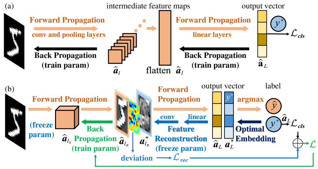
Figure 1: (a) Conventional back propagation training approach on CNN for image classification tasks. (b) Our hierarchical and decoupled post-training framework based on feature map reconstruction for image classification tasks.

With the vision of integrating both conceptions, this study develops a modularization evaluation and a hierarchical decoupled post-training framework for E2E architectures (Fig.1), aiming to enhance explainability and enable targeted optimization while retaining the superior performance of E2E models.

Considering their essential role in AD applications, this paper focuses on image classification tasks. Fig.2 illustrates that certain intermediate layers in a converged convolutional neural network (CNN) are independently post-trained, while the remaining modules are kept frozen. Specifically, the feature maps $\mathbf{a}_{l}^{\ast},l\in\{L,L-1,\cdots l_{R}\}$ are constructed layer by layer using the proposed optimal embedding algorithm (OE) and the feature reconstruction algorithms (FR), and the feature map $\mathbf{a}_{l}^{\ast}$ serves as the surrogate signal of the ground truth label $y^{\ast}$ at $l_{R}^{th}$ layer. The OE part seeks the reconstructed output vector $\mathbf{a}_{L}^{\ast}$ that is closest to the original forward output vector $\hat{\mathbf{a}}_{L}$ and satisfies $y^{\ast}=\arg\max_{i}(\mathbf{a}_{L}^{\ast})_{i}$, which we managed to find the optimum solution under L1 norm and L2 norm respectively. Then FR through linear or convolutional operations are executed layer by layer until achieving the $\mathbf{a}_{l_{R}}^{\ast}$.

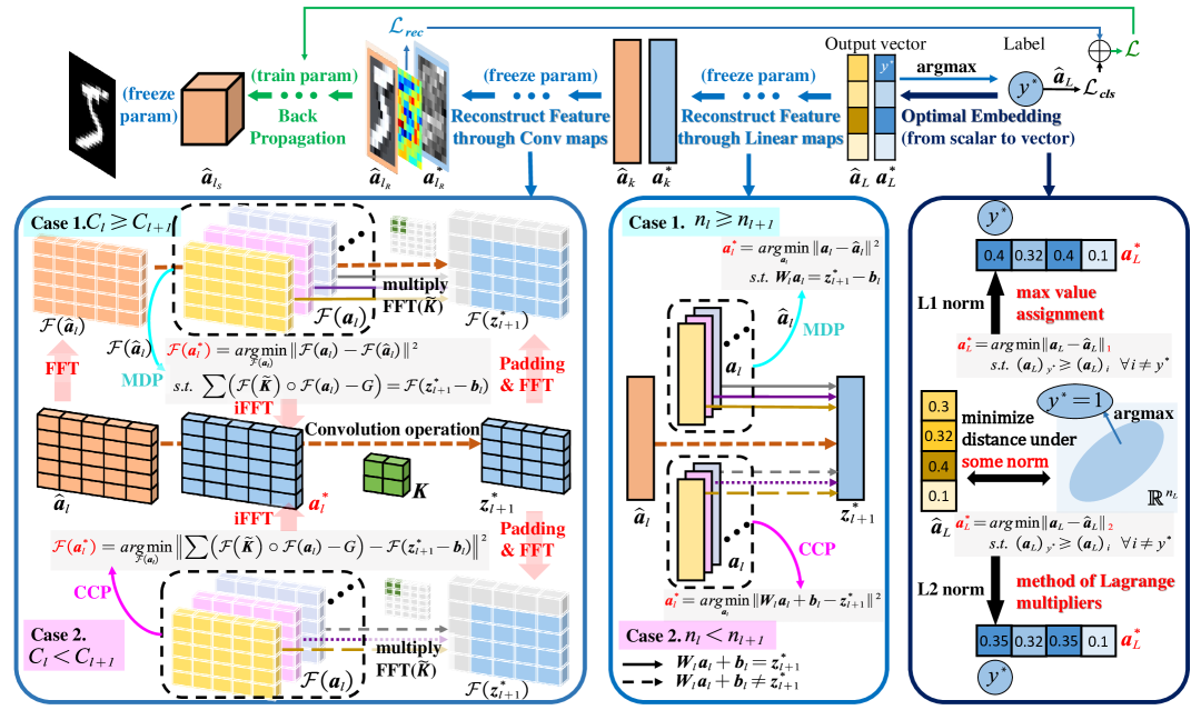
Figure 2: Hierarchical and Decoupled Post-Training based on Feature Map Reconstruction for Image Classification Tasks. Given a well-trained CNN, the optimal embedding and feature reconstruction are executed in line with the network’s backward computation flow to obtain the reconstructed $(l_{R})^{th}$ feature map. A combination of reconstruction loss and classification loss is then used to post-train the intermediate modules from $l_{S}^{th}$ layer to $l_{R}^{th}$ layer.

The FR processes are modeled as two types of optimization problems depending on whether the channel number $C_{l}$ (or vector dimension $n_{l}$) of the $l^{th}$ feature map is greater than the channel number $C_{l+1}$ (or vector dimension $n_{l+1}$) of the $(l+1)^{th}$ feature map or not. This dichotomy results from whether the desired $\mathbf{a}_{l_{R}}^{\ast}$ that satisfies network computation, is underdetermined (infinitely many solutions) or overdetermined (no exact solution). Subsequently, the deviation between the forward feature $\hat{\mathbf{a}}_{l_{R}}$ and the reconstructed feature $\mathbf{a}_{l_{R}}^{\ast}$ is defined as the reconstruction loss $\mathcal{L}_{rec}$. Modules from $l_{S}^{th}$ layer to $l_{R}^{th}$ layer are optimized via back propagation (BP) using a combination of $\mathcal{L}_{rec}$ and the final classification loss $\mathcal{L}_{cls}$.

Our contributions can be summarized as follows.

• We originally propose a post-training approach on the basis of FR-backpropagation to achieve targeted optimization, which also provides a novel feature map deviation visualization method to encourage explainability.

• The FR algorithm for linear operations is skillfully designed. Guided by optimization theory, solving a systems of linear equations or a least squares problem constitutes the majority of computation in this FR process.

• Informed by the FR for linear operations, the FR for convolutional operations is meticulously formalized, additionally leveraging fast Fourier transform (FFT) to substantially reduce computational cost.

• The optimal embedding that maps category labels to reconstructed output vectors is systematically discussed, and its precise optimum solutions under the L1 and L2 norm can be obtained efficiently.

2 Related Work

2.1 Decoupling Networks

Decoupled learning has been widely researched to address inefficiencies of lockings in BP approaches. Jaderberg et al. [9] developed decoupled neural interfaces, where synthetic gradients are used to decouple layer updates, allowing for asynchronous training of different modules. As a simpler yet more parallelizable alternative, decoupled greedy learning based on a greedy relaxation of the joint learning objective was later introduced [3]. Similarly, Zhuang et al. [40] explored delayed gradient updates to achieve a fully decoupled training scheme that can train modules independently, reducing memory overhead while maintaining competitive performance. Peng et al.[22] extended decoupled learning by incorporating re-computation and weight prediction strategies to mitigate memory explosion.

Beyond decoupled training, several works have partially decoupled deep networks by extracting comprehensible knowledge or instructive information for the purpose of improving interpretability. Li et al. [17] proposed Ego-Net to better estimate egocentric vehicle orientation by extracting meaningful intermediate geometrical representations. Odense and Garcez [20] proposed a layer-wise extraction method using M-of-N rules, demonstrating considerable explanations for certain layers, such as softmax layers. Furthermore, Zhang et al. [36] managed to train a feature map convergence evaluation network to quantitatively assess the training maturity of individual modules.

2.2 Explainable AI for AD systems

Over the past few years, researchers have extensively explored visualization methods to help understanding DNN outputs in classification or perception tasks. Class activation mapping (CAM), introduced by Zhou et al. [39], highlights class-specific influential regions to explain model decisions. Simonyan et al. [26] proposed gradient-based visualization methods for class saliency maps across various CNNs. This work laid the foundation for Grad-CAM [25], an extension version of CAM introduced by Selvaraju et al.. Besides, Jiang et al. [10] further advanced this by proposing LayerCAM, which integrates hierarchical class activation maps to refine localization accuracy. Furthermore, Shapley value-based CAM [37] obtains the importance of each pixel through the Shapley values. Zeiler and Fergus [35] introduced a deconvolutional network to project feature activations back to the input pixel space, giving insight into the function of intermediate feature layers. OD-XAI [18] utilized Grad-CAM and saliency maps to locate the important regions that contribute to semantic road segmentation. Abukmeil et al.[1] proposed the first explainable semantic segmentation model for AD based on the variational autoencoder, which used multiscale second-order derivatives between the latent space and the encoder layers to capture the curvatures of the neurons’ responses. For LiDAR-based 3D object detection, OccAM’s Laser [24] serves as a perturbation-based approach empirically estimates the importance of each point by testing the model with randomly generated subsets of the input point cloud without requiring any prior knowledge of model architectures or parameters. Gou et al. [7] developed a visual analytics system equipped with a disentangled representation learning and semantic adversarial learning, to assess, understand, and improve traffic light detection. Moreover, interactive software that allows real-time inspection of neuron activations, and a high-quality feature visualization method via regularized optimization are helpful in inspiring intuition [34].

Regarding planning and prediction tasks, the generated explanations rely on attention mechanisms either as part of the transformer architecture or in conjunction with a recurrent neural network (RNN) [16]. Jiang et al. [11] proposed an intention-aware interactive transformer model to address the problem of real-time vehicle trajectory prediction in large-scale dense traffic scenarios. Kochakarn et al. [14] proposed a self-supervision pipeline with the attention mechanisms that can create spatial and temporal heatmaps on the scene graphs, to infer representative and well-separated embeddings. Wang et al. [28] presented a method for intention prediction of surrounding vehicles using a bidirectional long short term memory network combined with a conditional random field layer, which can find the characteristics that contribute the most to the prediction.

These state-of-the-art techniques greatly improve the explainability of AI in AD tasks and can be deployed into existing decision-making systems [16]. However, they still face the sharp trade-off between computational overhead and performance, since the interpretation monitor is supposed to not take too much time to operate [32]. In addition, these explainable algorithms may fail to correctly capture the crucial attributes that are responsible for degraded outputs due to their modeling defects [16].

3 Method

Consider a pretrained baseline CNN with its weight $\mathbf{W}_{l}$ and bias $\mathbf{b}_{l}$ for each $l^{th}$ layer, $l\in\{1,2,...,L\}$. Denote the $l^{th}$ preactivated feature by $\hat{\mathbf{z}}_{l}$, and the $l^{th}$ activated feature by $\hat{\mathbf{a}}_{l}=activate(\mathbf{z}_{l})$, which satisfies $\hat{\mathbf{z}}_{l+1}=\mathbf{W}_{l}\hat{\mathbf{a}}_{l}+\mathbf{b}_{l}$. In general, we assume that the linear weight matrix $\mathbf{W}_{l}$ is always full-rank in all subsequent analyses.

The post-train of the modules from the $l_{S}^{th}$ layer to the $l_{R}^{th}$ layer can be performed by optimizing the following loss $\mathcal{L}$, where the core and crux of FR-PT lies in how to reconstruct the feature maps $\mathbf{a}_{l_{R}}^{\ast}$ from final labels appropriately and efficiently.

$$\mathcal{L}_{cls}=CrossEntropy(\mathbf{y}^{\ast},\hat{\mathbf{a}}_{L})$$ (1)

$$\mathcal{L}_{rec}=MSE(\mathbf{a}_{l_{R}}^{\ast},\hat{\mathbf{a}}_{l_{R}})$$ (2)

$$\mathcal{L}=(1-\alpha)\mathcal{L}_{cls}+\alpha\mathcal{L}_{rec}$$ (3)

We adopt a greedy strategy to reconstruct all feature maps from $\mathbf{a}_{L}^{\ast}$ to $\mathbf{a}_{l_{R}}^{\ast}$ layer by layer. That is, each reconstruction step from $\mathbf{z}_{l+1}^{\ast}$ and parameters at the $l^{th}$ layer, pursues the ”best” $\mathbf{a}_{l}^{\ast}$ without considering other feature maps, resulting in the obtained $\mathbf{a}_{l}^{\ast}$ may not be the optimal choice for successive determinations of feature maps $\mathbf{a}_{k}^{\ast}$, where $k<l$.

Since multiple operations are commonly involved in CNNs, we divide them into linear operations, convolutional operations, the ”argmax” operation, and other operations in the following discussion. Before giving concrete algorithms, we need to analyze the reverse computation of linear operations at the single $l^{th}$ layer. During the transformation from $\hat{\mathbf{a}}_{l}$ to $\hat{\mathbf{z}}_{l+1}$, the feature channels either expand or contract, which makes the linear system $\mathbf{W}_{l}\mathbf{a}_{l}^{\ast}+\mathbf{b}_{l}=\mathbf{z}_{l+1}^{\ast}$ either unsolvable or underdetermined, respectively. In order to cope with the first case, the computing consistency principle (CCP) is proposed to determine the feature $\mathbf{a}_{l}^{\ast}$ that minimizes the computing consistency error $\|\mathbf{W}_{l}\mathbf{a}_{l}^{\ast}+\mathbf{b}_{l}-\mathbf{z}_{l+1}^{\ast}\|$ as the reconstructed feature. In regard of the second case, the minimal deviation principle (MDP) is proposed to prefer the feature $\mathbf{a}_{l}^{\ast}$ that minimizes the deviation degree $\|\mathbf{a}_{l}^{\ast}-\hat{\mathbf{a}}_{l}\|$ among all features that satisfy the linear computation $\mathbf{W}_{l}\mathbf{a}_{l}^{\ast}+\mathbf{b}_{l}=\mathbf{z}_{l+1}^{\ast}$, as the reconstructed feature. Both principles choose the feature $\mathbf{a}_{l}^{\ast}$ in a way that can mostly inherit the superiority capability of former converged network computation, that is, leverage the exceptional achievement of E2E overall optimization.

3.1 Feature Reconstruction through Linear Operations

Given the reconstructed $(l+1)^{th}$ preactivation feature map $\mathbf{z}_{l+1}^{\ast}$ with dimension $n_{l+1}$, the frozen linear weights $\mathbf{W}_{l}$, bias $\mathbf{b}_{l}$, and the original $l^{th}$ activated feature $\hat{\mathbf{a}}_{l}$ with dimension $n_{l}$, the reconstructed $l^{th}$ activated feature $\mathbf{a}_{l}^{\ast}$ is desired. Adhere to the architecture of the baseline CNN, one can choose either of the following cases to perform.

(a) $n_{l}\geq n_{l+1}$. Among the infinitely many solutions $\mathbf{a}_{l}$ satisfying $W_{l}\mathbf{a}_{l}+\mathbf{b}_{l}=\mathbf{z}_{l+1}^{\ast}$, the one closest to the original version $\mathbf{a}_{l}$ is preferred as the reconstructed feature $\mathbf{a}_{l}^{\ast}$ according to MDP. For each instance $x$, Eq. 4 provides a strict convex quadratic programming with linear constraints.

$$\mathbf{a}_{l}^{\ast}=\arg\min_{\mathbf{a}_{l}} \|\mathbf{a}_{l}-\hat{\mathbf{a}}_{l}\|^{2}$$

s.t. $$W_{l}\mathbf{a}_{l}=\mathbf{z}_{l+1}^{\ast}-\mathbf{b}_{l}\phantom{+c^{2}}$$ (4)

Dual method [5] is applied to solve Eq. 4. The Lagrangian function is $L(\mathbf{a}_{l},\boldsymbol{\lambda})=\|\mathbf{a}_{l}-\hat{\mathbf{a}}_{l}\|^{2}-\boldsymbol{\lambda}(\hat{\mathbf{a}}_{l}\mathbf{W}_{l}+\mathbf{b}_{l}-\mathbf{z}_{l+1}^{\ast})$, where $\boldsymbol{\lambda}\in\mathbb{R}^{n_{l+1}}$ is the Lagrange multiplier. Set its partial derivative to zero as Eq. 5.

$$\frac{\partial L}{\partial\boldsymbol{\lambda}}(\mathbf{a}_{l}^{\ast},\boldsymbol{\lambda}^{\ast})=\mathbf{0},\quad\frac{\partial L}{\partial\mathbf{a}_{l}}(\mathbf{a}_{l}^{\ast},\boldsymbol{\lambda}^{\ast})=\mathbf{0}$$ (5)

Write these two equations in $(n_{l}+n_{l+1})$-dimensional matrix form as Eq. 6.

$$\begin{pmatrix}{2\mathbb{I}_{n_{l}}}&{-\mathbf{W}_{l}^{T}}\\ {\mathbf{W}_{l}}&{\mathbf{0}_{n_{l+1}}}\end{pmatrix}\begin{pmatrix}{\mathbf{a}_{l}^{\ast}}\\ {\boldsymbol{\lambda}^{\ast}}\end{pmatrix}=\begin{pmatrix}{2\hat{\mathbf{a}}_{l}}\\ {\mathbf{z}_{l+1}^{\ast}-\mathbf{b}_{l}}\end{pmatrix},\forall x$$ (6)

Since $\mathbf{W}_{l}$ is full-rank matrix, the left matrix is full-rank, suggesting that there exists an unique solution $(\mathbf{a}_{l}^{\ast},\boldsymbol{\lambda}^{\ast})\in\mathbb{R}^{n_{l}+n_{l+1}}$.

(b) $n_{l}<n_{l+1}$. The $\mathbf{a}^{\ast}_{l}$ with minimal squared error of the computing consistency is pursued, thereby yielding for a least squares problem 7.

$$\mathbf{a}_{l}^{\ast}=\arg\min_{\mathbf{a}_{l}}\|\mathbf{W}_{l}\mathbf{a}_{l}+\mathbf{b}_{l}-\mathbf{z}_{l+1}^{\ast}\|^{2},\forall x$$ (7)

Both the system of linear equations 6 and the least squares problem 7 have been well-studied, and can be solved efficiently using standard numerical methods.

3.2 Feature Reconstruction through Convolutional Operations

Given the reconstructed $(l+1)^{th}$ pre-activated feature $\mathbf{z}_{l+1}^{\ast}\in\mathbb{R}^{BS\times C_{l+1}\times H_{l+1}\times W_{l+1}}$, the frozen convolutinal kernel $\mathbf{K}_{l}$, bias $\mathbf{b}_{l}$, and the original $l^{th}$ activated feature map $\hat{\mathbf{a}}_{l}\in\mathbb{R}^{BS\times C_{l}\times H_{l}\times W_{l}}$, the reconstructed $l^{th}$ activated feature $\mathbf{a}_{l}^{\ast}$ is desired. For engineering convenience, this study focuses primarily on the case where the convolutional kernels use stride 1 and no padding (i.e., $stride=1,padding=0$). Under this setting, the feature map sizes satisfy $H_{l}>H_{l+1}$ and $W_{l}>W_{l+1}$.

As a variety of linear transformation, the reconstruction of convolutional operation can be solved by formulae in Section 3.1. However, due to the larger feature map size and the multiplexing of convolutional kernels $\mathbf{K}_{l}$, this method can be highly computationally expensive. To deal with this, we designed an algorithm based on FFT and convolution theorem to significantly reduce computing complexity while causing negligible additional modeling error.

Let $T_{n,m}^{x}$ be the contribution from the $m^{th}$ channel of feature map $\hat{\mathbf{a}_{l}}$ to the $n^{th}$ channel of feature map $\hat{\mathbf{z}}_{l+1}$ for instance $x$. The “$\otimes$” in Eq. 8 implies convolutional operation in neural networks.

$$T_{n,m}^{x}=\hat{\mathbf{a}}_{l}[x,m]\otimes\mathbf{K}[n,m]\in\mathbb{R}^{H_{l+1}\times W_{l+1}}$$ (8)

Thus, the $n^{th}$ channel of $\hat{\mathbf{z}}_{l+1}$ for instance $x$ is given by Eq. 9.

$$\hat{\mathbf{z}}_{l+1}[x,n]=\sum_{m=1}^{C_{l}}T_{n,m}^{x}+(\mathbf{b}_{l})_{n}$$ (9)

To utilize the convolution theorem, $\mathcal{F}(f)\mathcal{F}(g)=\mathcal{F}(f\ast g)$, the operation in convolutional layer ”$\otimes$” needs to be replaced by convolution in mathematical version ”$\ast$”. Thus the original convolutional kernel $\mathbf{K}$ needs to be flipped as the following $\widetilde{\mathbf{K}}\in\mathbb{R}^{H_{\mathbf{K}}\times{W}_{\mathbf{K}}}$.

$$\widetilde{\mathbf{K}}[n,m](s,t)=K[n,m](H_{\mathbf{K}}-1-s,W_{\mathbf{K}}-1-t)$$ (10)

Hence, we have formula 3.2. Note that the”$\ast$” here is not standard mathematical notation for convolution in neural networks do not regard tensors as functions on infinite spaces, which means the boundary needs further processing.

$$T_{n,m}^{x}(i,j)= \sum_{s=1}^{H_{\mathbf{K}}}\sum_{t=1}^{W_{\mathbf{K}}}\hat{\mathbf{a}}_{l}[x,m](i+s,j+t)\mathbf{K}[n,m](s,t)$$

$$= \sum_{s^{\prime}=1}^{H_{\mathbf{K}}}\sum_{t^{\prime}=1}^{W_{\mathbf{K}}}\hat{\mathbf{a}}_{l}[x,m]\scriptstyle(i+H_{\mathbf{K}}-1-s^{\prime},j+W_{\mathbf{K}}-1-t^{\prime})\cdot$$

$$\widetilde{\mathbf{K}}[n,m](s^{\prime},t^{\prime})$$

$$= \hat{\mathbf{a}}_{l}[x,m]\ast\widetilde{\mathbf{K}}[n,m]\in\mathbb{R}^{H_{l+1}\times W_{l+1}}$$ (11)

The Fourier transforms of $\widetilde{\mathbf{K}}[n,m]$, $\hat{\mathbf{a}}_{l}[x,m]$, and $T_{n,m}^{x}$ are Eq. 12, 13, and 3.2, respectively, where $i$ refers to the imaginary unit. With the goal to preserve all information, we zero-pad $T_{n,m}^{x}$ on the left and top, and $\widetilde{\mathbf{K}}[n,m]$ on the right and bottom, so as to make $\mathcal{F}(\widetilde{\mathbf{K}}[n,m])$ and $\mathcal{F}(T_{n,m}^{x})$ match the shape of $\mathcal{F}(\hat{\mathbf{a}}_{l}[x,m])$.

$$\mathcal{F}(\widetilde{\mathbf{K}}[n,m])(u,v)=\sum_{s=1}^{H_{\mathbf{K}}}\sum_{t=1}^{W_{\mathbf{K}}}\widetilde{\mathbf{K}}[n,m](s,t)e^{-2\pi i(\frac{us}{H_{l}}+\frac{vt}{W_{l}})}$$ (12)

$$\mathcal{F}(\hat{\mathbf{a}}_{l}[x,m])(u,v)=\sum_{k=1}^{H_{l}}\sum_{j=1}^{W_{l}}\hat{\mathbf{a}}_{l}[x,m](k,j)e^{-2\pi i(\frac{uk}{H_{l}}+\frac{vj}{W_{l}})}$$ (13)

$$\mathcal{F}(T_{n,m}^{x})(u,v)$$

$$= \sum_{k=1}^{H_{l+1}}\sum_{j=1}^{W_{l+1}}T_{m}^{b,n}(k,j)e^{-2\pi i(\frac{u(k+H_{\mathbf{K}}-1)}{H_{l}}+\frac{v(j+W_{\mathbf{K}}-1)}{W_{l}})}$$

$$= \sum_{k=1}^{H_{l+1}}\sum_{j=1}^{W_{l+1}}\sum_{s=1}^{H_{\mathbf{K}}}\sum_{t=1}^{W_{\mathbf{K}}}\hat{\mathbf{a}}_{l}[x,m]\scriptstyle(k+H_{\mathbf{K}}-1-s,j+W_{\mathbf{K}}-1-t)\cdot$$

$$\widetilde{K}[n,m](s,t)e^{-2\pi i(\frac{u(k+H_{\mathbf{K}}-1)}{H_{l}}+\frac{v(j+W_{\mathbf{K}}-1)}{W_{l}})}$$ (14)

Due to the finiteness of feature map size, the boundary of feature maps needs further modification using Eq. 3.2, where set $B_{s,t}$ for each $(s,t)\in H_{\mathbf{K}}\times W_{\mathbf{K}}$ contains all boundary elements in $\hat{\mathbf{a}}_{l}$ that $T_{n,m}^{x}$ does not count while $\mathcal{F}(\hat{\mathbf{a}}_{l}[x,m])\circ\mathcal{F}(\widetilde{\mathbf{K}}[n,m])$ does, as shown in Fig.3.

$$G_{n,m}^{x}[\hat{\mathbf{a}}_{l}[x,m]] (u,v)=\sum_{s=1}^{H_{\mathbf{K}}}\sum_{t=1}^{W_{\mathbf{K}}}\sum_{(k,j)\in B_{s,t}}\widetilde{\mathbf{K}}[n,m](s,t)\cdot$$

$$\hat{\mathbf{a}}_{l}[x,m](k,j)e^{-2\pi i(\frac{u(s+k)}{H_{l}}+\frac{v(t+j)}{W_{l}})}$$ (15)

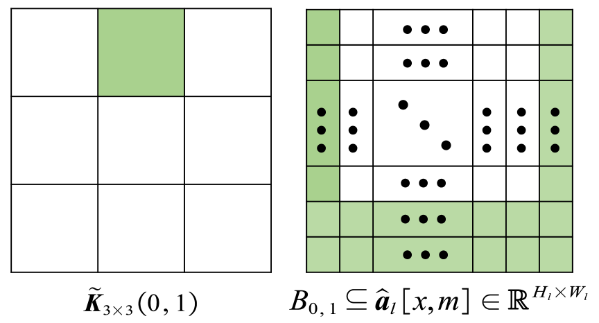
Figure 3: Schematic diagram of the boundary set $B_{0,1}$ for $\widetilde{\mathbf{K}}(0,1)$.

Thereupon, one can verify the network computing $\mathbf{a}_{l}^{\ast}[x,m]\otimes\mathbf{K}[n,m]=T_{n,m}^{x}[\mathbf{a}_{l}^{\ast}]$ is equivalent to equation 16, where ”$\circ$” is element-wise multiplication.

$$\mathcal{F}(\mathbf{a}_{l}^{\ast}[x,m])\circ\mathcal{F}(\widetilde{\mathbf{K}}[n,m])-G_{n,m}^{x}[\mathbf{a}_{l}^{\ast}]=\mathcal{F}(T_{n,m}^{x}[\mathbf{a}_{l}^{\ast}])$$ (16)

Since Fourier transform is linear, the desired newtork computation (Eq. 9)is equivalent to Eq. 3.2 for any $n\in C_{l+1}$ and any instance $x$.

$$\mathcal{F}(\mathbf{z}_{l+1}^{\ast}[x,n]-(\mathbf{b}_{l})_{n})=\sum_{m=1}^{C_{l}}\mathcal{F}(T_{n,m}^{x}[\mathbf{a}_{l}^{\ast}])$$

$$= \sum_{m=1}^{C_{l}}\{\mathcal{F}(\mathbf{a}_{l}^{\ast}[x,m])\circ\mathcal{F}(\widetilde{\mathbf{K}}[n,m])-G_{n,m}^{x}[\mathbf{a}_{l}^{\ast}]\}$$ (17)

In real computing, the $G_{n,m}^{x}[\mathbf{a}_{l}^{\ast}]$ is replaced by $G_{n,m}^{x}[\hat{\mathbf{a}}_{l}]$, leading formula 3.2 to be approximately correct.

(a) $C_{l}\geq C_{l+1}$. We need to solve a convex quadratic programming 3.2 established by the MDP, for each $(u,v)\in H_{l}\times W_{l}$ and each instance $x$.

$$\min_{\mathcal{F}(\mathbf{a}_{l}[x,m])}\sum_{m=1}^{C_{l}}\|\mathcal{F}(\mathbf{a}_{l}[x,m])(u,v)-\mathcal{F}(\hat{\mathbf{a}}_{l}[x,m])(u,v)\|^{2}$$

$$\text{s.t.}\quad\sum_{m=1}^{C_{l}}(\mathcal{F}(\mathbf{a}_{l}[x,m])\circ\mathcal{F}(\widetilde{\mathbf{K}}[n,m])-G^{x}_{n,m}[\hat{\mathbf{a}}_{l}])(u,v)$$

$$=\mathcal{F}(\mathbf{z}_{l+1}^{\ast}[x,n]-(\mathbf{b}_{l})_{n})(u,v),n=1,2,\cdots,C_{l+1}$$ (18)

According to Eq. 6, the linear system 19 can be built for each $(u,v)\in H_{l}\times W_{l}$ and each instance $x$, producing the $\mathcal{F}(\mathbf{a}_{l}^{\ast}[x,m])(u,v),m=1,2,\cdots,C_{l}$ each time.

$$\begin{pmatrix}\mathbb{I}_{C_{l}}&\mathcal{F}(\mathbf{\tilde{K}})^{T}\\ \mathcal{F}(\widetilde{\mathbf{K}})&\mathbf{0}_{C_{l+1}}\end{pmatrix}\begin{pmatrix}\mathcal{F}(\mathbf{a}_{l}^{\ast})\\ \frac{-1}{2}\boldsymbol{\lambda}^{\ast}\end{pmatrix}=\begin{pmatrix}\mathcal{F}(\hat{\mathbf{a}_{l}})\\ \scalebox{0.8}{$\mathcal{F}(\mathbf{z}_{l+1}^{\ast}-(\mathbf{b}_{l})_{n})+\sum_{m=1}^{C_{l}}G_{n,m}^{x}$}\end{pmatrix}$$ (19)

(b) $C_{l}<C_{l+1}$. We need to solve a least square problem 20 established by the CCP, for each $(u,v)\in H_{l}\times W_{l}$ and each instance $x$. $\mathcal{F}(\mathbf{a}_{l}^{\ast}[x,m])(u,v),m=1,2,\cdots,C_{l}$ can be obtained each time.

$$\min_{\mathcal{F}(\mathbf{a}_{l})}\|\sum_{m=1}^{C_{l}}(\mathcal{F}(\widetilde{\mathbf{K}})\circ\mathcal{F}(\mathbf{a}_{l})-G_{n,m}^{x}[\hat{\mathbf{a}}_{l}])-\mathcal{F}(\mathbf{z}_{l+1}^{\ast}-(\mathbf{b}_{l})_{n})\|^{2}$$ (20)

Finally, since Fourier transform is an isometry, i.e., it preserves distances in the L2 norm such that $\|\mathcal{F}(\mathbf{x})-\mathcal{F}(\mathbf{y})\|_{L_{2}}=\|\mathbf{x}-\mathbf{y}\|_{L_{2}}$, the desired reconstructed feature map $\mathbf{a}_{l}^{\ast}$ can be directly obtained by applying the inverse FFT to $\mathcal{F}(\mathbf{a}_{l}^{\ast})$.

3.3 Optimal Embedding for Category Labels

Obviously, there are infinitely many output vector candidates whose argmax corresponds to the correct category label. According to MDP, the optimal output vector reconstruction $\mathbf{a}^{\ast}_{L}$ can be seeked by solving problem 21, where $\|\cdot\|_{{N}}$ denotes some type of norm, and $(\mathbf{a}_{L})_{k}$ denotes the $k^{th}$ entry of vector $\mathbf{a}_{L}$. In this section, we will discuss this problem under L1 and L2 norms.

$$\min_{\mathbf{a}_{L}} \|\mathbf{a}_{L}-\hat{\mathbf{a}}_{L}\|_{N}$$ (21)

$$s.t. (\mathbf{a}_{L})_{y^{\ast}}\geq(\mathbf{a}_{L})_{i},\forall i\in I_{y^{\ast}}=\{1,2,\cdots,n_{L}\}-\{y^{\ast}\}$$

(a). A trivial solution called ”Maximum Assignment (MA)” 22, simply assigns the maximum value to the ground-truth label $(y^{\ast})^{th}$ entry.

$$(\mathbf{a}^{MA}_{L})_{j}=\begin{cases}\max_{i}(\hat{\mathbf{a}}_{L})_{i},&\text{when }j=y^{\ast}\\ (\hat{\mathbf{a}}_{L})_{j},&\text{otherwise}\end{cases}$$ (22)

proposition: When $\|\cdot\|_{{N}}$ is set to the L1 norm, MA solution $\mathbf{a}_{L}^{MA}$ is the optimal output vector reconstruction $\mathbf{a}^{\ast}_{L}$.
Proof. MA solution $\mathbf{a}_{L}^{MA}$ satisfies the constrait condition in problem 21. It suffices to check whether the MA solution has the minimum norm. The L1 norm is the sum of absolute values of all entries. For any $\mathbf{a}_{L}$ satisfying $(\mathbf{a}_{L})_{y^{\ast}}=\max_{i}(\mathbf{a}_{L})_{i}$, formula 23 holds.

$$\|\mathbf{a}_{L}-\hat{\mathbf{a}}_{L}\|_{L_{1}}\geq\max_{i}(\hat{\mathbf{a}_{L}})_{i}-(\hat{\mathbf{a}}_{L})_{y^{\ast}}=\|\mathbf{a}_{L}^{MA}-\hat{\mathbf{a}}_{L}\|_{L_{1}}$$ (23)

This completes the proof. $\blacksquare$

(b). When $\|\cdot\|_{{N}}$ is set to the L2 norm, we introduce Lagrangian multipliers $\boldsymbol{\mu}\in\mathbb{R}^{n_{L}-1}$ for constraints in problem 21. For any $\mu_{i}=0$, the corresponding constraint is not active, i.e., $(\mathbf{a}_{L})_{y^{\ast}}>(\mathbf{a}_{L})_{i}$, while when $\mu_{i}>0$, the corresponding constraint is active, i.e., $(\mathbf{a}_{L})_{y^{\ast}}=(\mathbf{a}_{L})_{i}$. The Lagrangian function is as follows.

$$L(\mathbf{a}_{L},\boldsymbol{\mu})=\mathbf{a}_{L}^{T}\mathbf{a}_{L}-2\mathbf{a}_{L}^{T}\hat{\mathbf{a}}_{L}+\hat{\mathbf{a}}_{L}^{T}\hat{\mathbf{a}}_{L}-\sum_{i\in I_{y^{\ast}}}\mu_{i}[(\mathbf{a}_{L})_{y^{\ast}}-(\mathbf{a}_{L})_{i}]$$ (24)

Since problem 21 is a convex quadratic problem satisfying Slater’s condition [5], it has a unique solution $\mathbf{a}_{L}^{\ast}$. Hence, there exists a unique solution $(\mathbf{a}_{L}^{\ast},\boldsymbol{\mu}^{\ast})$ for the KKT conditions 25e.

$$(\mathbf{a}_{L}^{\ast})_{y^{\ast}}\geq\max_{i}(\mathbf{a}_{L}^{\ast})_{i}$$ (25a)

$$\boldsymbol{\mu}^{\ast}\succeq 0$$ (25b)

$$\frac{\partial L}{\partial(\mathbf{a}_{L}^{\ast})_{y^{\ast}}}(\mathbf{a}_{L}^{\ast},\boldsymbol{\mu}^{\ast})=2(\mathbf{a}_{L}^{\ast}-\hat{\mathbf{a}}_{L})_{y^{\ast}}-\sum_{i\in I_{y^{\ast}}}\mu_{i}^{\ast}=0$$ (25c)

$$\frac{\partial L}{\partial(\mathbf{a}_{L}^{\ast})_{i}}(\mathbf{a}_{L}^{\ast},\boldsymbol{\mu}^{\ast})=2(\mathbf{a}_{L}^{\ast}-\hat{\mathbf{a}}_{L})_{i}+\mu_{i}^{\ast}=0$$ (25d)

$$\mu_{i}^{\ast}[(\mathbf{a}_{L}^{\ast})_{y^{\ast}}-(\mathbf{a}_{L}^{\ast})_{i}]=0,\forall i\in I_{y^{\ast}}$$ (25e)

According to condition 25e c and d, we can eliminate $\mathbf{a}_{L}^{\ast}$ by

$$(\mathbf{a}_{L}^{\ast})_{y^{\ast}}=(\hat{\mathbf{a}}_{L})_{y^{\ast}}+\frac{\sum_{i\in I_{y^{\ast}}}\mu_{i}^{\ast}}{2}$$ (26)

$$(\mathbf{a}_{L}^{\ast})_{i}=(\hat{\mathbf{a}}_{L})_{i}-\frac{\mu_{i}^{\ast}}{2},\forall i\in I_{y^{\ast}}$$ (27)

It is clear that $(\mathbf{a}_{L}^{\ast})_{y^{\ast}}\geq(\hat{\mathbf{a}}_{L})_{y^{\ast}}$ and $(\mathbf{a}_{L}^{\ast})_{i}\leq(\hat{\mathbf{a}}_{L})_{i}\forall i\in I_{y^{\ast}}$. The KKT condition 25e suffices to solve all ${\mu}_{i}^{\ast}$, which we split into three cases:

(i) For all $i\in I_{1}=\{i|(\hat{\mathbf{a}}_{L})_{y^{\ast}}\geq(\hat{\mathbf{a}}_{L})_{i}\}$, the $i^{th}$ entry of vector $(\mathbf{a}_{L}^{\ast})_{i}$ can contribute zero to the L2 norm difference by letting $\mu^{\ast}_{i}=0$ and $(\mathbf{a}_{L}^{\ast})_{i}=(\hat{\mathbf{a}}_{L})_{i}$.

(ii) For all $i\in I_{2}=\{i|(\hat{\mathbf{a}}_{L})_{y^{\ast}}<(\hat{\mathbf{a}}_{L})_{i},(\mathbf{a}_{L}^{\ast})_{y^{\ast}}>(\mathbf{a}_{L}^{\ast})_{i}\}$, we get inequation 28 by Eq. 26, Eq. 27 and $\mu_{i}^{\ast}=0$ by condition 25e e.

$$\frac{\sum_{k\in I_{y^{\ast}}}\mu_{k}^{\ast}}{2}>(\mathbf{a}^{\ast}_{L})_{i}-(\hat{\mathbf{a}}_{L})_{y^{\ast}}=(\hat{\mathbf{a}}_{L})_{i}-(\hat{\mathbf{a}}_{L})_{y^{\ast}}$$ (28)

(iii) The ”active set” $I_{3}=\{i|(\hat{\mathbf{a}}_{L})_{y^{\ast}}<(\hat{\mathbf{a}}_{L})_{i},(\mathbf{a}_{L}^{\ast})_{y^{\ast}}=(\mathbf{a}_{L}^{\ast})_{i}\}$ suggests $\boldsymbol{\mu}^{\ast}_{I_{3}}\succ 0$ and the corresponding constraints are active. For all $i\in I_{3}$ we have Eq. 29 by Eq. 26 and 27.

$$\frac{\sum_{k}\mu_{k}^{\ast}}{2}+\frac{\mu_{i}^{\ast}}{2}=(\hat{\mathbf{a}}_{L})_{i}-(\hat{\mathbf{a}}_{L})_{y^{\ast}}$$ (29)

That is, $(\mathbf{1}_{|I_{3}|}+\mathbb{I}_{|I_{3}|})\frac{\boldsymbol{\mu}^{\ast}_{I_{3}}}{2}=((\hat{\mathbf{a}}_{L})_{i}-(\hat{\mathbf{a}}_{L})_{y^{\ast}})_{I_{3}}$. Through matrix inversion, equation 30 will hold, where $\mathbb{I}_{|I_{3}|}$ indicates the $|I_{3}|$-dimensional identity matrix, and $\mathbf{1}_{|I_{3}|}$ indicates the $|I_{3}|$-dimensional matrix with all entries equal to 1.

$$\frac{\boldsymbol{\mu}^{\ast}_{I_{3}}}{2}=(\mathbb{I}_{|I_{3}|}-\frac{\mathbf{1}_{|I|_{3}}}{|I_{3}|+1})((\hat{\mathbf{a}}_{L})_{i}-(\hat{\mathbf{a}}_{L})_{y^{\ast}})_{I_{3}}$$ (30)

Therefore, as long as the sets $I_{1}$, $I_{2}$ and $I_{3}$ are determined, we can obtain $\boldsymbol{\mu}^{\ast}$ and thus $\mathbf{a}_{L}^{\ast}$. The index set $I_{1}$ is straightforward to identify, whereas $I_{2}$ and $I_{3}$ must be considered jointly. By summing Eq. 29 over all $i\in I_{3}$, we obtain Eq. 31.

$$\frac{\sum_{k\in I_{y^{\ast}}}\mu_{k}^{\ast}}{2}=\frac{\sum_{k\in I_{3}}[(\hat{\mathbf{a}}_{L})_{k}-(\hat{\mathbf{a}}_{L})_{y^{\ast}}]}{|I_{3}|+1}$$ (31)

Hence, for all $j\in I_{2},i\in I_{3}$, we have inequation 32 by formula 28, 29, and 31.

$$(\hat{\mathbf{a}}_{L})_{j}-(\hat{\mathbf{a}}_{L})_{y^{\ast}}<\frac{\sum_{k\in I_{3}}[(\hat{\mathbf{a}}_{L})_{k}-(\hat{\mathbf{a}}_{L})_{y^{\ast}}]}{|I_{3}|+1}<(\hat{\mathbf{a}}_{L})_{i}-(\hat{\mathbf{a}}_{L})_{y^{\ast}}$$ (32)

Let $\{d_{s}=(\hat{\mathbf{a}}_{L})_{t_{s}}-(\hat{\mathbf{a}}_{L})_{y^{\ast}}\}_{t_{s}\in I_{2}\cup I_{3}}$ be a monotonically decreasing sequence. It is easy to get $(\hat{\mathbf{a}}_{L})_{j}<(\hat{\mathbf{a}}_{L})_{i},\forall j\in I_{2},i\in I_{3}$. Thus, we can determine set $I_{2}$ and $I_{3}$ in $\{d_{s}\}$ by rewriting equation 32 as follows.

$$(|I_{3}|+1)d_{|I_{3}|+1}<\sum_{s=1}^{|I_{3}|}d_{s}<(|I_{3}|+1)d_{|I_{3}|}$$ (33)

Due to the existence and uniqueness of the Lagrange multipliers $\boldsymbol{\mu}^{\ast}$, there must exist a unique number of $|I_{3}|$, which can be achieved by checking all indices $\{1,2,\cdots,|I_{2}|+|I_{3}|\}$ against formula 33. Then, we have $I_{3}=\{t_{s}\}_{s=1}^{|I_{3}|}$. We call the obtained $\mathbf{a}_{L}^{\ast}$ ”nearest embedding” solution $\mathbf{a}_{L}^{NE}$.

Algorithm 1 Parallelizable Nearest Embedding Algorithm

0: original output vector $\hat{\mathbf{a}}_{L}$ and ground truth label $y^{\ast}$

0: reconstructed output vector $\mathbf{a}_{L}^{NE}$

1: $\mathbf{a}_{L}^{NE}\leftarrow\hat{\mathbf{a}}_{L}$

2: Get the difference sequence $\{d_{i}\}_{i=1}^{n_{L}}$, where $d_{i}\leftarrow(\hat{\mathbf{a}}_{L})_{i}-(\hat{\mathbf{a}}_{L})_{y^{\ast}}$.

3: Sort $\{d_{i}\}_{i=1}^{n_{L}}$ to get the monotonically decreasing sequence $\{d_{s}\}_{i=1}^{n_{L}}$, where $d_{s}\leftarrow(\hat{\mathbf{a}}_{L})_{t_{s}}-(\hat{\mathbf{a}}_{L})_{y^{\ast}}$.

4: Get the cumulate sum $\{c_{w}\}$, where $c_{w}\leftarrow\sum_{s=1}^{w}d_{s}$.

5: Get sequences $\{s\cdot d_{s}\}$ and $\{(s+1)\cdot d_{s}\}$.

6: Find the unique index $s=|I_{3}|$ that satisfies $d_{|I_{3}|}>0$ and formula 33.

7: Get index set $I_{3}\leftarrow\{t_{s}\}_{s=1}^{|I_{3}|}$ and calculate $\boldsymbol{\mu}^{\ast}_{I_{3}}$ by equation 30. Set other $\mu_{i}^{\ast}\leftarrow 0$.

8: Update $\mathbf{a}_{L}^{NE}$ by equations 26 and 27.

9: return  $\mathbf{a}_{L}^{NE}$

3.4 Other Reverse Operations

We next discuss the reverse computation of other operations classically occurred in CNNs.

(a) Non-linear Activation. Common activation functions mapping $\mathbf{z}_{l}$ to $\mathbf{a}_{l}$ can be divided into three types:

(i) Bijection with unlimited range (e.g. leaky relu, sinh, arcsinh). Their inverse functions has domain of $\mathbb{R}$, naturally suitable for the reverse computation sending $\mathbf{a}_{l}^{\ast}$ to $\mathbf{z}_{l}^{\ast}$.

(ii) Bijection with limited range (e.g. sigmoid, arctan). $\mathbf{a}_{l}^{\ast}$ may not within the domain of these activations’ inverse functions. Hence, we firstly limit $\mathbf{a}_{l}^{\ast}$ to fit the domain of their inverse functions, and then perform the reverse computation.

Table 1: modules post-training results of a baseline on Mnist with test accuracy $97.62\%$ (loss coefficient $\alpha=0.1$)

PT ($l_{S},l_{R}$)	#paras	GPU Mem	epoch1	epoch5	epoch10
BP(0,1)	52	7.93	$97.693_{\pm 0.035}$	$97.671_{\pm 0.062}$	$\mathbf{97.719_{\pm 0.054}}$
FR(0,1)	52	8.23	$97.682_{\pm 0.042}$	$97.688_{\pm 0.037}$	$97.692_{\pm 0.039}$
BP(0,2)	256	7.93	$97.703_{\pm 0.031}$	$97.707_{\pm 0.038}$	$\mathbf{97.748_{\pm 0.023}}$
FR(0,2)	256	8.20	$97.682_{\pm 0.040}$	$97.707_{\pm 0.026}$	$97.739_{\pm 0.021}$
BP(1,2)	204	5.37	$97.700_{\pm 0.022}$	$97.712_{\pm 0.018}$	$97.694_{\pm 0.022}$
FR(1,2)	204	5.64	$97.695_{\pm 0.020}$	$97.697_{\pm 0.018}$	$\mathbf{97.716_{\pm 0.028}}$
BP(0,3)	2826	7.96	$97.736_{\pm 0.030}$	$97.855_{\pm 0.054}$	$\mathbf{97.913_{\pm 0.062}}$
FR(0,3)	2826	7.98	$97.676_{\pm 0.036}$	$97.744_{\pm 0.047}$	$97.781_{\pm 0.058}$
BP(1,3)	2774	5.40	$97.727_{\pm 0.065}$	$97.833_{\pm 0.072}$	$\mathbf{97.901_{\pm 0.047}}$
FR(1,3)	2774	5.41	$97.695_{\pm 0.045}$	$97.748_{\pm 0.057}$	$97.791_{\pm 0.031}$
BP(2,3)	2570	5.39	$97.718_{\pm 0.046}$	$97.826_{\pm 0.023}$	$\mathbf{97.852_{\pm 0.036}}$
FR(2,3)	2570	5.41	$97.692_{\pm 0.047}$	$97.742_{\pm 0.023}$	$97.741_{\pm 0.034}$

Table 2: modules post-training results of a baseline on Cifar10 with test accuracy $62.55\%$ (loss coefficient $\alpha=0.1$)

PT ($l_{S},l_{R}$)	#paras	GPU Mem	epoch1	epoch5	epoch10
BP(0,1)	380	17.43	$62.474_{\pm 0.173}$	$62.568_{\pm 0.256}$	$62.667_{\pm 0.244}$
FR(0,1)	380	20.45	$62.336_{\pm 0.326}$	$62.584_{\pm 0.472}$	$\mathbf{62.722_{\pm 0.288}}$
BP(0,2)	840	17.43	$62.546_{\pm 0.202}$	$62.569_{\pm 0.321}$	$\mathbf{62.736_{\pm 0.226}}$
FR(0,2)	840	19.60	$62.371_{\pm 0.323}$	$62.420_{\pm 0.183}$	$62.600_{\pm 0.241}$
BP(1,2)	460	12.01	$\mathbf{62.698_{\pm 0.155}}$	$62.674_{\pm 0.109}$	$62.622_{\pm 0.084}$
FR(1,2)	460	13.94	$62.667_{\pm 0.085}$	$62.684_{\pm 0.095}$	$62.603_{\pm 0.122}$
BP(0,3)	2205	17.45	$62.294_{\pm 0.399}$	$62.717_{\pm 0.253}$	$62.749_{\pm 0.177}$
FR(0,3)	2205	19.46	$62.465_{\pm 0.254}$	$62.637_{\pm 0.283}$	$\mathbf{62.755_{\pm 0.386}}$
BP(1,3)	1825	12.03	$62.662_{\pm 0.125}$	$62.719_{\pm 0.141}$	$\mathbf{62.775_{\pm 0.203}}$
FR(1,3)	1825	13.79	$62.576_{\pm 0.102}$	$62.696_{\pm 0.143}$	$62.653_{\pm 0.103}$
BP(2,3)	1365	12.02	$62.564_{\pm 0.146}$	$\mathbf{62.593_{\pm 0.183}}$	$62.498_{\pm 0.114}$
FR(2,3)	1365	13.08	$62.505_{\pm 0.102}$	$62.543_{\pm 0.145}$	$62.575_{\pm 0.161}$
BP(0,4)	33053	17.81	$62.415_{\pm 0.375}$	$62.654_{\pm 0.433}$	$62.711_{\pm 0.549}$
FR(0,4)	33053	19.65	$62.393_{\pm 0.313}$	$62.693_{\pm 0.194}$	$\mathbf{62.982_{\pm 0.215}}$
Bp(1,4)	32673	12.38	$62.451_{\pm 0.265}$	$62.700_{\pm 0.184}$	$62.682_{\pm 0.177}$
FR(1,4)	32673	13.99	$62.481_{\pm 0.148}$	$62.856_{\pm 0.242}$	$\mathbf{62.883_{\pm 0.120}}$
BP(2,4)	32213	12.37	$62.383_{\pm 0.236}$	$62.639_{\pm 0.220}$	$62.533_{\pm 0.199}$
FR(2,4)	32213	13.28	$62.544_{\pm 0.185}$	$\mathbf{62.656_{\pm 0.143}}$	$62.587_{\pm 0.109}$
BP(3,4)	30848	12.35	$62.526_{\pm 0.256}$	$62.691_{\pm 0.084}$	$\mathbf{62.715_{\pm 0.122}}$
FR(3,4)	30848	13.26	$62.535_{\pm 0.143}$	$62.703_{\pm 0.091}$	$62.692_{\pm 0.145}$
BP(0,5)	34343	17.95	$62.137_{\pm 0.244}$	$62.588_{\pm 0.442}$	$62.583_{\pm 0.319}$
FR(0,5)	34343	19.51	$62.239_{\pm 0.305}$	$62.631_{\pm 0.230}$	$\mathbf{62.878_{\pm 0.198}}$
BP(1,5)	33963	12.40	$62.369_{\pm 0.290}$	$\mathbf{62.807_{\pm 0.305}}$	$62.582_{\pm 0.112}$
FR(1,5)	33963	13.84	$62.340_{\pm 0.239}$	$62.695_{\pm 0.143}$	$62.719_{\pm 0.200}$
BP(2,5)	33503	12.39	$62.360_{\pm 0.215}$	$\mathbf{62.612_{\pm 0.174}}$	$62.445_{\pm 0.190}$
FR(2,5)	33503	13.13	$62.384_{\pm 0.197}$	$62.586_{\pm 0.242}$	$62.544_{\pm 0.163}$
BP(3,5)	32138	12.37	$62.383_{\pm 0.109}$	$\mathbf{62.579_{\pm 0.116}}$	$62.447_{\pm 0.149}$
FR(3,5)	32138	13.11	$62.348_{\pm 0.188}$	$62.568_{\pm 0.239}$	$62.522_{\pm 0.170}$
BP(4,5)	1290	12.02	$62.301_{\pm 0.152}$	$\mathbf{62.365_{\pm 0.111}}$	$62.260_{\pm 0.071}$
FR(4,5)	1290	12.76	$62.263_{\pm 0.104}$	$62.309_{\pm 0.154}$	$62.272_{\pm 0.053}$

(iii) Not bijection with limited range (e.g. relu, sin). We choose identity map as relu’s reverse compute. As for locally bijective functions like sin, $\mathbf{a}_{l}^{\ast}$ is normalized into $[-1,1]$ and then deactivated by their inverse functions.

(b) Pooling Layers (stride=kernel size). Since the information lost during pooling operations contributes little to the final output, we reconstruct the pre-pooling feature maps by directly copying values from the post-pooling ones.

4 Experiments

Table 3: modules post-training results of a baseline on Cifar100 with test accuracy $36.74\%$ (loss coefficient $\alpha=0.7$)

PT ($l_{S},l_{R}$)	#paras	GPU Mem	epoch1	epoch5	epoch10
BP(0,1)	760	26.51	$36.806_{\pm 0.269}$	$36.901_{\pm 0.214}$	$\mathbf{36.972_{\pm 0.199}}$
FR(0,1)	760	34.18	$36.957_{\pm 0.224}$	$36.661_{\pm 0.386}$	$36.904_{\pm 0.250}$
BP(0,2)	2125	26.53	$36.846_{\pm 0.265}$	$\mathbf{36.858_{\pm 0.172}}$	$36.780_{\pm 0.216}$
FR(0,2)	2125	30.95	$36.695_{\pm 0.345}$	$36.785_{\pm 0.237}$	$36.515_{\pm 0.449}$
BP(1,2)	1365	19.83	$\mathbf{37.158_{\pm 0.127}}$	$37.090_{\pm 0.089}$	$37.072_{\pm 0.136}$
FR(1,2)	1365	22.70	$37.005_{\pm 0.158}$	$36.990_{\pm 0.094}$	$37.058_{\pm 0.083}$
BP(0,3)	4845	26.56	$36.594_{\pm 0.272}$	$36.455_{\pm 0.183}$	$36.329_{\pm 0.300}$
FR(0,3)	4845	30.66	$36.814_{\pm 0.229}$	$36.930_{\pm 0.259}$	$\mathbf{37.045_{\pm 0.324}}$
BP(1,3)	4085	19.87	$36.905_{\pm 0.138}$	$36.771_{\pm 0.122}$	$36.626_{\pm 0.160}$
FR(1,3)	4085	22.40	$37.042_{\pm 0.206}$	$37.120_{\pm 0.245}$	$\mathbf{37.198_{\pm 0.118}}$
BP(2,3)	2720	19.85	$37.082_{\pm 0.117}$	$36.932_{\pm 0.077}$	$36.734_{\pm 0.068}$
FR(2,3)	2720	22.38	$37.108_{\pm 0.148}$	$\mathbf{37.197_{\pm 0.112}}$	$37.100_{\pm 0.089}$
BP(0,4)	87021	27.50	$36.366_{\pm 0.255}$	$36.243_{\pm 0.394}$	$35.941_{\pm 0.193}$
FR(0,4)	87021	31.51	$\mathbf{36.759_{\pm 0.178}}$	$36.543_{\pm 0.267}$	$36.464_{\pm 0.249}$
BP(1,4)	86261	20.81	$36.809_{\pm 0.196}$	$36.659_{\pm 0.122}$	$36.319_{\pm 0.160}$
FR(1,4)	86261	23.25	$\mathbf{36.866_{\pm 0.216}}$	$36.839_{\pm 0.168}$	$36.666_{\pm 0.107}$
BP(2,4)	84896	20.79	$\mathbf{36.932_{\pm 0.136}}$	$36.706_{\pm 0.171}$	$36.429_{\pm 0.133}$
FR(2,4)	84896	23.23	$36.895_{\pm 0.140}$	$36.816_{\pm 0.137}$	$36.725_{\pm 0.109}$
BP(3,4)	82176	20.76	$37.063_{\pm 0.113}$	$37.029_{\pm 0.178}$	$36.923_{\pm 0.149}$
FR(3,4)	82176	23.19	$\mathbf{37.191_{\pm 0.100}}$	$37.081_{\pm 0.159}$	$37.084_{\pm 0.173}$
BP(0,5)	112721	27.80	$36.109_{\pm 0.289}$	$35.852_{\pm 0.324}$	$35.531_{\pm 0.578}$
FR(0,5)	112721	31.56	$36.865_{\pm 0.117}$	$37.007_{\pm 0.332}$	$\mathbf{37.179_{\pm 0.138}}$
BP(1,5)	111961	21.10	$36.426_{\pm 0.249}$	$36.427_{\pm 0.273}$	$35.561_{\pm 0.202}$
FR(1,5)	111961	23.29	$36.957_{\pm 0.092}$	$37.116_{\pm 0.113}$	$\mathbf{37.215_{\pm 0.155}}$
BP(2,5)	110596	21.08	$36.562_{\pm 0.223}$	$36.606_{\pm 0.206}$	$35.758_{\pm 0.141}$
FR(2,5)	110596	23.28	$36.962_{\pm 0.231}$	$37.007_{\pm 0.150}$	$\mathbf{37.038_{\pm 0.157}}$
BP(3,5)	107876	21.05	$36.801_{\pm 0.239}$	$36.738_{\pm 0.183}$	$36.463_{\pm 0.112}$
FR(3,5)	107876	23.24	$37.040_{\pm 0.076}$	$37.042_{\pm 0.106}$	$\mathbf{37.108_{\pm 0.099}}$
BP(4,5)	25700	20.11	$36.999_{\pm 0.088}$	$37.069_{\pm 0.143}$	$36.995_{\pm 0.128}$
FR(4,5)	25700	22.30	$37.050_{\pm 0.112}$	$\mathbf{37.087_{\pm 0.086}}$	$37.065_{\pm 0.069}$

To evaluate FR-based post-training (FR-PT), experiments on six classical image classification benchmarks are conducted. We choose a 2Conv+1fc architecture as the baseline network for Mnist, a 3Conv+2fc for Cifar-10, a 3Conv+2fc for Cifar-100, a 4Conv+2fc for Tiny ImageNet, a 5Conv+2fc for ImageNette, and a 5Conv+2fc for ImageWoof.

Data sets are all instance normalized as the default setting following the previous works [29]. All nonlinear activation functions are ”tanh”. The pooling layers are configured as max-pooling, with their stride equal to the kernel size. The optimizer for BP is Adam with a learning rate $0.001$. The batch size is set to 256 for all training processes. The performance of each network is evaluated by its test accuracy ($\%$).

Table 4: modules post-training results of a baseline on Tiny ImageNet with test accuracy $24.99\%$ (loss coefficient $\alpha=0.7$)

PT ($l_{S},l_{R}$)	#paras	GPU Mem	epoch1	epoch5	epoch10
BP(0,1)	760	137.26	$24.945_{\pm 0.186}$	$\mathbf{25.187_{\pm 0.159}}$	$25.100_{\pm 0.206}$
FR(0,1)	760	171.37	$24.533_{\pm 0.232}$	$24.724_{\pm 0.165}$	$24.829_{\pm 0.160}$
BP(0,2)	3035	139.30	$25.408_{\pm 0.486}$	$\mathbf{25.412_{\pm 0.518}}$	$25.413_{\pm 0.291}$
FR(0,2)	3035	157.21	$25.373_{\pm 0.336}$	$25.368_{\pm 0.254}$	$25.375_{\pm 0.445}$
BP(1,2)	2275	109.77	$25.116_{\pm 0.383}$	$25.511_{\pm 0.342}$	$25.427_{\pm 0.306}$
FR(1,2)	2275	136.53	$25.365_{\pm 0.533}$	$\mathbf{25.697_{\pm 0.442}}$	$25.339_{\pm 0.464}$
BP(0,3)	10945	139.79	$25.264_{\pm 0.447}$	$\mathbf{25.455_{\pm 0.368}}$	$25.430_{\pm 0.452}$
FR(0,3)	10945	150.54	$25.216_{\pm 0.344}$	$25.144_{\pm 0.702}$	$25.199_{\pm 0.439}$
BP(1,3)	10185	109.46	$25.013_{\pm 0.391}$	$25.523_{\pm 0.313}$	$25.270_{\pm 0.457}$
FR(1,3)	10185	129.06	$\mathbf{25.618_{\pm 0.350}}$	$25.098_{\pm 0.694}$	$25.587_{\pm 0.480}$
BP(2,3)	7910	106.57	$\mathbf{25.702_{\pm 0.314}}$	$25.663_{\pm 0.337}$	$25.647_{\pm 0.287}$
FR(2,3)	7910	119.06	$25.624_{\pm 0.170}$	$25.521_{\pm 0.286}$	$25.502_{\pm 0.306}$
BP(0,4)	25165	140.19	$25.072_{\pm 0.597}$	$25.092_{\pm 0.642}$	$24.805_{\pm 0.363}$
FR(0,4)	25165	150.09	$25.189_{\pm 0.734}$	$25.334_{\pm 0.544}$	$\mathbf{25.713_{\pm 0.498}}$
BP(1,4)	24405	109.63	$25.072_{\pm 0.554}$	$24.942_{\pm 0.547}$	$24.531_{\pm 0.363}$
FR(1,4)	24405	127.44	$25.439_{\pm 0.474}$	$25.303_{\pm 0.634}$	$\mathbf{25.523_{\pm 0.378}}$
BP(2,4)	22130	106.73	$25.372_{\pm 0.447}$	$25.078_{\pm 0.481}$	$25.005_{\pm 0.371}$
FR(2,4)	22130	117.78	$25.533_{\pm 0.614}$	$\mathbf{25.698_{\pm 0.416}}$	$25.377_{\pm 0.303}$
BP(3,4)	14220	106.64	$25.696_{\pm 0.341}$	$25.462_{\pm 0.213}$	$25.442_{\pm 0.225}$
FR(3,4)	14220	116.77	$25.601_{\pm 0.298}$	$25.717_{\pm 0.242}$	$\mathbf{25.945_{\pm 0.299}}$
BP(0,5)	394317	143.84	$25.341_{\pm 0.534}$	$25.151_{\pm 0.418}$	$24.288_{\pm 0.263}$
FR(0,5)	394317	153.10	$\mathbf{26.408_{\pm 0.349}}$	$26.117_{\pm 0.698}$	$25.474_{\pm 0.358}$
BP(1,5)	393557	113.96	$25.528_{\pm 0.427}$	$24.694_{\pm 0.483}$	$23.529_{\pm 0.369}$
FR(1,5)	393557	130.46	$25.861_{\pm 0.313}$	$\mathbf{25.979_{\pm 0.342}}$	$25.403_{\pm 0.282}$
BP(2,5)	391282	111.49	$25.547_{\pm 0.328}$	$25.001_{\pm 0.443}$	$23.829_{\pm 0.292}$
FR(2,5)	391282	121.79	$\mathbf{26.346_{\pm 0.250}}$	$25.883_{\pm 0.342}$	$25.380_{\pm 0.285}$
BP(3,5)	383372	112.46	$26.031_{\pm 0.371}$	$25.454_{\pm 0.233}$	$24.526_{\pm 0.244}$
FR(3,5)	383372	121.69	$\mathbf{26.410_{\pm 0.261}}$	$26.097_{\pm 0.191}$	$25.434_{\pm 0.321}$
BP(4,5)	369152	111.87	$\mathbf{26.779_{\pm 0.194}}$	$26.173_{\pm 0.159}$	$25.539_{\pm 0.195}$
FR(4,5)	369152	121.77	$26.421_{\pm 0.140}$	$26.391_{\pm 0.144}$	$26.068_{\pm 0.176}$
BP(0,6)	496917	144.96	$24.824_{\pm 0.606}$	$23.969_{\pm 0.338}$	$21.866_{\pm 0.213}$
FR(0,6)	496917	153.55	$25.885_{\pm 0.222}$	$\mathbf{26.359_{\pm 0.149}}$	$26.104_{\pm 0.401}$
BP(1,6)	496157	114.50	$24.592_{\pm 0.472}$	$23.707_{\pm 0.461}$	$21.342_{\pm 0.376}$
FR(1,6)	496157	131.68	$\mathbf{26.008_{\pm 0.284}}$	$25.934_{\pm 0.365}$	$25.968_{\pm 0.155}$
BP(2,6)	493882	114.05	$24.780_{\pm 0.568}$	$23.588_{\pm 0.295}$	$21.456_{\pm 0.298}$
FR(2,6)	493882	122.63	$25.883_{\pm 0.223}$	$\mathbf{26.116_{\pm 0.208}}$	$26.055_{\pm 0.213}$
BP(3,6)	485972	112.99	$25.504_{\pm 0.267}$	$24.258_{\pm 0.267}$	$21.780_{\pm 0.237}$
FR(3,6)	485972	122.54	$25.925_{\pm 0.206}$	$\mathbf{26.008_{\pm 0.151}}$	$25.846_{\pm 0.204}$
BP(4,6)	471752	112.28	$25.826_{\pm 0.257}$	$24.655_{\pm 0.337}$	$22.908_{\pm 0.187}$
FR(4,6)	471752	122.37	$\mathbf{26.079_{\pm 0.166}}$	$26.061_{\pm 0.228}$	$26.014_{\pm 0.128}$
BP(5,6)	102600	108.57	$25.630_{\pm 0.186}$	$25.148_{\pm 0.221}$	$24.283_{\pm 0.252}$
FR(5,6)	102600	117.48	$25.686_{\pm 0.144}$	$\mathbf{25.807_{\pm 0.214}}$	$25.794_{\pm 0.151}$

Section 4.1 compares FR-based post-training (FR-PT) with the SOTA BP-based post-training (BP-PT) across six benchmarks, and visualizes the deviations between the forward and reconstructed feature maps. Section 4.2 demonstrates ablation experiments to verify the necessary of optimal embedding methods. Section 4.3 studies the effect of FR-PT on networks at different training stages. Lastly, we discuss the effectiveness of FR-PT on different network architectures in Section 4.4.

Table 5: modules post training results of a baseline on ImageNette with test accuracy $51.56\%$ (loss coefficient $\alpha=0.3$)

PT ($l_{S},l_{R}$)	#paras	GPU Mem	epoch1	epoch5	epoch10
BP(0,1)	18760	1320.80	$50.652_{\pm 0.455}$	$51.399_{\pm 0.419}$	$51.554_{\pm 0.435}$
FR(0,1)	18760	1600.61	$50.978_{\pm 0.595}$	$51.490_{\pm 0.755}$	$\mathbf{51.651_{\pm 0.589}}$
BP(0,2)	62125	1321.29	$50.983_{\pm 0.512}$	$51.427_{\pm 0.446}$	$51.850_{\pm 0.306}$
FR(0,2)	62125	1491.10	$51.238_{\pm 0.236}$	$51.608_{\pm 0.365}$	$\mathbf{51.939_{\pm 0.488}}$
BP(1,2)	43365	1074.74	$51.544_{\pm 0.169}$	$51.806_{\pm 0.301}$	$51.954_{\pm 0.200}$
FR(1,2)	43365	1239.19	$51.503_{\pm 0.201}$	$51.704_{\pm 0.207}$	$\mathbf{52.010_{\pm 0.300}}$
BP(0,3)	98445	1369.04	$50.601_{\pm 0.553}$	$51.429_{\pm 0.671}$	$51.911_{\pm 0.599}$
FR(0,3)	98445	1460.55	$50.678_{\pm 0.564}$	$51.511_{\pm 0.364}$	$\mathbf{52.217_{\pm 0.432}}$
BP(1,3)	79685	1075.16	$51.282_{\pm 0.351}$	$52.048_{\pm 0.466}$	$52.194_{\pm 0.346}$
FR(1,3)	79685	1211.42	$51.567_{\pm 0.404}$	$51.939_{\pm 0.339}$	$\mathbf{52.336_{\pm 0.165}}$
BP(2,3)	36320	1074.66	$51.470_{\pm 0.205}$	$51.669_{\pm 0.368}$	$51.521_{\pm 0.368}$
FR(2,3)	36320	1211.07	$51.671_{\pm 0.102}$	$\mathbf{51.814_{\pm 0.270}}$	$51.794_{\pm 0.243}$
BP(0,4)	110970	1369.18	$50.150_{\pm 0.560}$	$51.024_{\pm 0.756}$	$\mathbf{52.183_{\pm 0.532}}$
FR(0,4)	110970	1454.04	$50.668_{\pm 0.660}$	$51.791_{\pm 0.329}$	$52.150_{\pm 0.418}$
BP(1,4)	92210	1075.31	$51.478_{\pm 0.653}$	$51.903_{\pm 0.495}$	$\mathbf{52.201_{\pm 0.440}}$
FR(1,4)	92210	1205.89	$51.289_{\pm 0.397}$	$51.936_{\pm 0.262}$	$52.061_{\pm 0.380}$
BP(2,4)	48845	1074.81	$51.208_{\pm 0.239}$	$51.712_{\pm 0.432}$	$\mathbf{52.064_{\pm 0.259}}$
FR(2,4)	48845	1204.80	$51.697_{\pm 0.356}$	$51.569_{\pm 0.318}$	$51.916_{\pm 0.318}$
BP(3,4)	12525	1074.39	$51.439_{\pm 0.340}$	$\mathbf{51.712_{\pm 0.255}}$	$51.496_{\pm 0.238}$
FR(3,4)	12525	1204.40	$51.468_{\pm 0.322}$	$51.575_{\pm 0.304}$	$51.534_{\pm 0.251}$
BP(0,5)	117750	1369.26	$49.934_{\pm 0.872}$	$51.557_{\pm 0.657}$	$\mathbf{52.275_{\pm 0.491}}$
FR(0,5)	117750	1453.52	$50.288_{\pm 0.588}$	$51.651_{\pm 0.529}$	$52.005_{\pm 0.580}$
BP(1,5)	98990	1075.39	$51.378_{\pm 0.527}$	$51.908_{\pm 0.267}$	$\mathbf{52.301_{\pm 0.289}}$
FR(1,5)	98990	1205.44	$51.409_{\pm 0.433}$	$52.270_{\pm 0.342}$	$52.265_{\pm 0.421}$
BP(2,5)	55625	1074.89	$51.205_{\pm 0.552}$	$51.814_{\pm 0.299}$	$\mathbf{52.176_{\pm 0.336}}$
FR(2,5)	55625	1204.33	$51.315_{\pm 0.391}$	$51.707_{\pm 0.138}$	$52.000_{\pm 0.513}$
BP(3,5)	19305	1074.47	$51.722_{\pm 0.343}$	$51.575_{\pm 0.291}$	$51.676_{\pm 0.372}$
FR(3,5)	19305	1203.91	$51.404_{\pm 0.419}$	$51.674_{\pm 0.402}$	$\mathbf{51.789_{\pm 0.280}}$
BP(4,5)	6780	1074.32	$51.600_{\pm 0.237}$	$51.901_{\pm 0.110}$	$\mathbf{52.120_{\pm 0.188}}$
FR(4,5)	6780	1203.78	$51.717_{\pm 0.197}$	$52.082_{\pm 0.215}$	$52.076_{\pm 0.118}$
BP(0,6)	179318	1369.97	$49.343_{\pm 0.749}$	$50.874_{\pm 0.684}$	$51.233_{\pm 0.971}$
FR(0,6)	179318	1453.65	$50.107_{\pm 0.817}$	$50.803_{\pm 0.497}$	$\mathbf{51.462_{\pm 0.420}}$
BP(1,6)	160558	1076.09	$50.668_{\pm 0.518}$	$51.496_{\pm 0.442}$	$51.073_{\pm 0.316}$
FR(1,6)	160558	1205.68	$51.139_{\pm 0.390}$	$\mathbf{51.687_{\pm 0.656}}$	$51.287_{\pm 0.495}$
BP(2,6)	117193	1075.59	$50.563_{\pm 0.610}$	$51.121_{\pm 0.600}$	$50.780_{\pm 0.392}$
FR(2,6)	117193	1204.57	$51.083_{\pm 0.579}$	$\mathbf{51.439_{\pm 0.469}}$	$50.996_{\pm 0.309}$
BP(3,6)	80873	1075.17	$51.011_{\pm 0.470}$	$51.050_{\pm 0.315}$	$51.124_{\pm 0.347}$
FR(3,6)	80873	1204.16	$\mathbf{51.389_{\pm 0.424}}$	$51.200_{\pm 0.342}$	$51.172_{\pm 0.278}$
BP(4,6)	68348	1075.03	$51.447_{\pm 0.420}$	$51.447_{\pm 0.250}$	$51.434_{\pm 0.362}$
FR(4,6)	68348	1204.01	$51.350_{\pm 0.433}$	$\mathbf{51.712_{\pm 0.333}}$	$51.468_{\pm 0.327}$
BP(5,6)	61568	1074.95	$51.654_{\pm 0.217}$	$51.755_{\pm 0.267}$	$51.592_{\pm 0.369}$
FR(5,6)	61568	1203.93	$51.524_{\pm 0.301}$	$\mathbf{51.664_{\pm 0.162}}$	$51.501_{\pm 0.222}$
BP(0,7)	180608	1369.98	$49.855_{\pm 0.542}$	$51.294_{\pm 0.351}$	$51.009_{\pm 0.483}$
FR(0,7)	180608	1453.49	$50.586_{\pm 0.627}$	$\mathbf{51.361_{\pm 0.602}}$	$51.129_{\pm 0.202}$
BP(1,7)	161848	1076.11	$50.665_{\pm 0.522}$	$51.159_{\pm 0.600}$	$50.280_{\pm 0.336}$
FR(1,7)	161848	1205.54	$51.101_{\pm 0.422}$	$\mathbf{51.366_{\pm 0.225}}$	$51.034_{\pm 0.202}$
BP(2,7)	118483	1075.61	$50.818_{\pm 0.359}$	$50.932_{\pm 0.369}$	$49.804_{\pm 0.386}$
FR(2,7)	118483	1204.43	$51.106_{\pm 0.475}$	$\mathbf{51.129_{\pm 0.354}}$	$50.736_{\pm 0.430}$
BP(3,7)	82163	1075.19	$51.118_{\pm 0.381}$	$51.004_{\pm 0.541}$	$50.466_{\pm 0.363}$
FR(3,7)	82163	1204.02	$51.177_{\pm 0.271}$	$\mathbf{51.190_{\pm 0.344}}$	$51.106_{\pm 0.312}$
BP(4,7)	69638	1075.05	$51.274_{\pm 0.232}$	$51.075_{\pm 0.286}$	$50.782_{\pm 0.317}$
FR(4,7)	69638	1203.87	$51.292_{\pm 0.226}$	$\mathbf{51.307_{\pm 0.197}}$	$51.238_{\pm 0.289}$
BP(5,7)	62858	1074.97	$51.264_{\pm 0.272}$	$51.350_{\pm 0.380}$	$50.889_{\pm 0.220}$
FR(5,7)	62858	1203.79	$51.389_{\pm 0.269}$	$\mathbf{51.468_{\pm 0.253}}$	$51.394_{\pm 0.218}$
BP(6,7)	1290	1074.26	$\mathbf{51.501_{\pm 0.190}}$	$51.468_{\pm 0.112}$	$51.192_{\pm 0.136}$
FR(6,7)	1290	1203.09	$51.409_{\pm 0.070}$	$51.340_{\pm 0.135}$	$51.126_{\pm 0.096}$

Table 6: modules post training results of a baseline on ImageWoof with test accuracy $27.23\%$ (loss coefficient $\alpha=0.1$)

PT ($l_{S},l_{R}$)	#paras	GPU Mem	epoch1	epoch5	epoch10
BP(0,1)	18760	1320.80	$\mathbf{27.255_{\pm 0.249}}$	$27.210_{\pm 0.178}$	$27.156_{\pm 0.210}$
FR(0,1)	18760	1606.72	$27.199_{\pm 0.279}$	$27.247_{\pm 0.236}$	$27.180_{\pm 0.170}$
BP(0,2)	62125	1321.29	$27.320_{\pm 0.320}$	$\mathbf{27.391_{\pm 0.329}}$	$27.381_{\pm 0.247}$
FR(0,2)	62125	1491.90	$27.109_{\pm 0.205}$	$27.246_{\pm 0.245}$	$27.368_{\pm 0.337}$
BP(1,2)	43365	966.78	$27.241_{\pm 0.192}$	$27.170_{\pm 0.145}$	$27.350_{\pm 0.253}$
FR(1,2)	43365	1101.77	$27.223_{\pm 0.307}$	$27.185_{\pm 0.197}$	$\mathbf{27.353_{\pm 0.219}}$
BP(0,3)	98445	1369.04	$27.218_{\pm 0.269}$	$\mathbf{27.414_{\pm 0.267}}$	$27.274_{\pm 0.359}$
FR(0,3)	98445	1461.20	$27.162_{\pm 0.241}$	$27.287_{\pm 0.189}$	$27.160_{\pm 0.296}$
BP(1,3)	79685	967.20	$\mathbf{27.413_{\pm 0.318}}$	$27.286_{\pm 0.321}$	$27.354_{\pm 0.224}$
FR(1,3)	79685	1069.39	$27.394_{\pm 0.335}$	$27.311_{\pm 0.344}$	$27.289_{\pm 0.272}$
BP(2,3)	36320	966.70	$27.460_{\pm 0.315}$	$27.490_{\pm 0.182}$	$27.437_{\pm 0.262}$
FR(2,3)	36320	1069.00	$27.455_{\pm 0.270}$	$27.462_{\pm 0.264}$	$\mathbf{27.554_{\pm 0.302}}$
BP(0,4)	110970	1369.18	$27.289_{\pm 0.332}$	$27.371_{\pm 0.343}$	$\mathbf{27.386_{\pm 0.443}}$
FR(0,4)	110970	1453.97	$27.185_{\pm 0.197}$	$27.228_{\pm 0.384}$	$27.111_{\pm 0.256}$
BP(1,4)	92210	967.35	$27.424_{\pm 0.356}$	$27.261_{\pm 0.403}$	$27.279_{\pm 0.311}$
FR(1,4)	92210	1062.41	$\mathbf{27.666_{\pm 0.336}}$	$27.447_{\pm 0.326}$	$27.231_{\pm 0.369}$
BP(2,4)	48845	966.85	$27.343_{\pm 0.230}$	$27.381_{\pm 0.181}$	$27.149_{\pm 0.303}$
FR(2,4)	48845	1061.90	$\mathbf{27.526_{\pm 0.253}}$	$27.381_{\pm 0.283}$	$27.198_{\pm 0.344}$
BP(3,4)	12525	966.43	$27.432_{\pm 0.273}$	$\mathbf{27.608_{\pm 0.243}}$	$27.539_{\pm 0.284}$
FR(3,4)	12525	1061.50	$27.587_{\pm 0.280}$	$27.559_{\pm 0.186}$	$27.470_{\pm 0.448}$
BP(0,5)	117750	1369.26	$27.137_{\pm 0.387}$	$26.778_{\pm 0.367}$	$26.709_{\pm 0.357}$
FR(0,5)	117750	1453.45	$27.088_{\pm 0.350}$	$\mathbf{27.190_{\pm 0.272}}$	$26.900_{\pm 0.402}$
BP(1,5)	98990	967.42	$27.231_{\pm 0.242}$	$27.302_{\pm 0.359}$	$26.679_{\pm 0.331}$
FR(1,5)	98990	1061.86	$\mathbf{27.478_{\pm 0.296}}$	$27.167_{\pm 0.481}$	$26.554_{\pm 0.426}$
BP(2,5)	55625	966.93	$27.244_{\pm 0.427}$	$27.098_{\pm 0.395}$	$26.801_{\pm 0.461}$
FR(2,5)	55625	1061.36	$\mathbf{27.577_{\pm 0.612}}$	$27.185_{\pm 0.430}$	$26.539_{\pm 0.293}$
BP(3,5)	19305	966.51	$27.378_{\pm 0.238}$	$27.294_{\pm 0.304}$	$27.193_{\pm 0.325}$
FR(3,5)	19305	1060.96	$\mathbf{27.630_{\pm 0.272}}$	$27.585_{\pm 0.339}$	$27.037_{\pm 0.231}$
BP(4,5)	6780	966.36	$27.849_{\pm 0.248}$	$27.468_{\pm 0.254}$	$27.292_{\pm 0.312}$
FR(4,5)	6780	1060.81	$\mathbf{27.903_{\pm 0.353}}$	$27.544_{\pm 0.120}$	$27.333_{\pm 0.215}$
BP(0,6)	179318	1369.97	$26.895_{\pm 0.589}$	$26.419_{\pm 0.593}$	$25.963_{\pm 0.555}$
FR(0,6)	179318	1453.64	$\mathbf{26.946_{\pm 0.489}}$	$26.681_{\pm 0.472}$	$25.513_{\pm 0.578}$
BP(1,6)	160558	968.13	$\mathbf{27.109_{\pm 0.381}}$	$26.472_{\pm 0.350}$	$25.772_{\pm 0.512}$
FR(1,6)	160558	1062.06	$26.918_{\pm 0.766}$	$26.589_{\pm 0.430}$	$25.826_{\pm 0.524}$
BP(2,6)	117193	967.63	$27.205_{\pm 0.506}$	$26.276_{\pm 0.452}$	$25.551_{\pm 0.299}$
FR(2,6)	117193	1061.56	$\mathbf{27.322_{\pm 0.354}}$	$26.416_{\pm 0.509}$	$25.976_{\pm 0.297}$
BP(3,6)	80873	967.21	$\mathbf{27.338_{\pm 0.346}}$	$26.821_{\pm 0.517}$	$25.991_{\pm 0.507}$
FR(3,6)	80873	1061.15	$27.310_{\pm 0.268}$	$26.679_{\pm 0.577}$	$26.259_{\pm 0.235}$
BP(4,6)	68348	967.07	$27.442_{\pm 0.381}$	$27.060_{\pm 0.347}$	$26.859_{\pm 0.491}$
FR(4,6)	68348	1061.00	$\mathbf{27.714_{\pm 0.349}}$	$27.256_{\pm 0.397}$	$27.004_{\pm 0.416}$
BP(5,6)	61568	966.99	$27.745_{\pm 0.227}$	$27.633_{\pm 0.250}$	$27.126_{\pm 0.215}$
FR(5,6)	61568	1060.92	$\mathbf{27.821_{\pm 0.326}}$	$27.587_{\pm 0.351}$	$27.129_{\pm 0.215}$
BP(0,7)	180608	1369.98	$\mathbf{27.394_{\pm 0.527}}$	$26.187_{\pm 0.419}$	$25.220_{\pm 0.646}$
FR(0,7)	180608	1453.49	$26.933_{\pm 0.645}$	$26.292_{\pm 0.483}$	$25.429_{\pm 0.517}$
BP(1,7)	161848	968.15	$27.043_{\pm 0.383}$	$26.215_{\pm 0.340}$	$25.345_{\pm 0.551}$
FR(1,7)	161848	1061.91	$\mathbf{27.088_{\pm 0.431}}$	$26.129_{\pm 0.327}$	$25.391_{\pm 0.702}$
BP(2,7)	118483	967.65	$27.121_{\pm 0.550}$	$26.172_{\pm 0.285}$	$25.004_{\pm 0.564}$
FR(2,7)	118483	1061.41	$\mathbf{27.205_{\pm 0.361}}$	$26.345_{\pm 0.301}$	$25.635_{\pm 0.508}$
BP(3,7)	82163	967.23	$\mathbf{27.345_{\pm 0.547}}$	$26.480_{\pm 0.292}$	$25.495_{\pm 0.448}$
FR(3,7)	82163	1060.99	$26.987_{\pm 0.509}$	$26.406_{\pm 0.387}$	$25.930_{\pm 0.395}$
BP(4,7)	69638	967.08	$27.442_{\pm 0.331}$	$26.691_{\pm 0.310}$	$26.103_{\pm 0.282}$
FR(4,7)	69638	1060.85	$\mathbf{27.539_{\pm 0.336}}$	$26.785_{\pm 0.468}$	$26.055_{\pm 0.224}$
BP(5,7)	62858	967.01	$27.343_{\pm 0.482}$	$26.941_{\pm 0.353}$	$26.513_{\pm 0.118}$
FR(5,7)	62858	1060.77	$\mathbf{27.613_{\pm 0.184}}$	$26.819_{\pm 0.489}$	$26.516_{\pm 0.529}$
BP(6,7)	1290	966.30	$\mathbf{27.742_{\pm 0.225}}$	$27.518_{\pm 0.095}$	$27.167_{\pm 0.116}$
FR(6,7)	1290	1060.06	$27.610_{\pm 0.206}$	$27.391_{\pm 0.090}$	$27.129_{\pm 0.196}$

4.1 Post-Training Results

We first define and train a baseline CNN architecture for each dataset, in which the number of channels in convolutional layers typically increases with depth, while the dimensionality of the subsequent fully connected layers decreases. To further improve the performance of converged CNNs pretrained by BP, this section compares FR-PT with the BP-based post-training, both starting with the same pretrained baseline CNN. Each training configuration is repeated for 10 runs to obtain statistically reliable performance results.

For each layer index $l\in\{1,2,\cdots,L\}$ in the original well-trained baseline network, we freeze the weights and bias parameters of all subsequent layers after the $l^{th}$ layer, and use algorithms described in Section 3 to generate the training datasets containing reconstructed feature maps $\mathbf{a}_{l}^{\ast}$ for all instances, where the nearest embedding $\mathbf{a}_{L}^{\ast}=\mathbf{a}_{L}^{NE}$ is adopted in the optimal embedding part sending scalar labels to output vectors. These priorly obtained datasets are directly used to compute the reconstruction loss $\mathcal{L}_{rec}$ (Eq. 2), as the parameters beyond the $l_{R}^{th}$ layer remain frozen during post-training processes.

During each FR-PT process, the first $l_{S}$ layers are frozen, indicating the total loss $\mathcal{L}$ (Eq. 3) is used to optimize the parameters between the $l_{S}^{th}$ layer and the $l_{R}^{th}$ layer. FR-PT is evaluated across all possible hyperparameter combinations $(l_{S},l_{R})$ for each baseline network architecture. The results are summarized in Tables 1-6 for each corresponding benchmark, including the number of trainable parameters, GPU memory jusage (MB), and the mean and standard deviation of test accuracy ($\%$).

It can be observed that FR-PT generally outperforms BP-PT when $l_{R}$ is set to the last few layer indices, such as $l_{R}=4$ for Cifar10 (Table 2); $l_{R}=3,4,5$ for Cifar100 (Table 3); $l_{R}=4,5,6$ for Tiny Imagenet (Table 4); $l_{R}=6,7$ for ImageNette (Table 5); $l_{R}=5$ for ImageWoof (Table 6), whereas BP-PT surpasses FR-PT when $l_{R}$ is set to the first few layer indices. The reason lies in the accumulation of information loss during the backward reverse computation, particularly due to reconstructions for pooling operations and convolutional operations with $C_{l}>C_{l+1}$. As a result, the reconstructed $y^{\ast}$-informed feature maps $\mathbf{a}^{\ast}_{l}$ at the first few layers deviate significantly from the original forward-obtained ones $\hat{\mathbf{a}}_{l}$ . This discrepancy leads to a larger violation of the pretrained parameters when optimizing the $\mathcal{L}_{rec}$ term, thereby disturbing the training process. As for Mnist, note the test accuracy of FR-PT is relatively lower than that of BP-PT on Mnist (Table 1). This may be attributed to the baseline network not being fully converged, allowing the BP method to continue improving performance effectively. Nevertheless, it is FR-PT that achieves the highest post-training generalization performance on CIFAR-10, CIFAR-100, ImageNette, and ImageWoof.

It is evident that independently training a module requires less GPU memory compared to training the entire network. Moreover, the GPU memory usages of FR-PT are slightly higher than those of BP-PT under the same module from $l_{S}$ to $l_{R})$, especially when $l_{R}$ is small, due to the additional storage of reconstructed feature maps required by FR-PT.

In addition to training networks, the feature reconstruct technique can also be used to visualize how intermediate feature maps evolve as the model’s capability improves. As shown in Fig. 4, the absolute values of $(\hat{\mathbf{a}}_{l}-\mathbf{a}_{l}^{\ast})$ become progressively more blue as the test accuracy grows, suggesting the discrepancy gets smaller and the network generates true outputs more consistently. Besides, it can be observed that the regular strip-shaped characteristic in discrepancy’s distribution is waning gradually, leaving weak noises that largely caused by the reconstruction modeling error. This phenomenon strongly supports our insight that the consistency between input-informed and label-informed intermediate representations is intrinsically positively associated with the evaluation of the models.

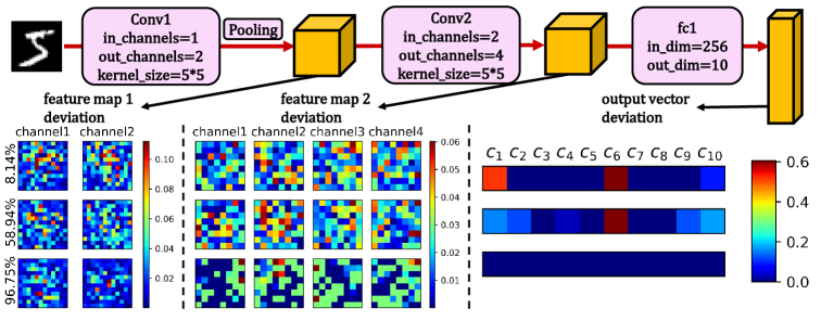
Figure 4: Absolute values of discrepancy between forward feature maps $\hat{\mathbf{a}}_{l}$ and reconstructed feature maps $\mathbf{a}_{l}^{\ast}$ as a single CNN evolves on Mnist at three training stages with test accuracy being $8.14\%$, $58.94\%$, and $96.75\%$.

Figure 5: Average test accuracy with $95\%$ confidence of optimal embedding approaches compared with one-hot coding across six benchmarks.

Figure 6: The post-training results comparison across 30 baselines with different training stages. A single baseline for Cifar100 evolves by one BP epoch per stage (black line). Then, for each post-training, only the parameters between $1^{th}$ layer and $4^{th}$ layer are trainable.

4.2 Ablation Study on Optimal Embedding

As for the transform from a scalar label $y^{\ast}$ to the output vector $\mathbf{a}_{L}^{\ast}$, we compared optimal embedding approaches $\mathbf{a}_{L}^{MA}$ and $\mathbf{a}_{L}^{NE}$ with the trivial one-hot code $\mathbf{a}_{L}^{OH}$ of true label. The reconstruction loss is $\mathcal{L}_{rec}=L1Loss(\hat{\mathbf{a}}_{L},\mathbf{a}_{L}^{MA})$, $\mathcal{L}_{rec}=MSE(\hat{\mathbf{a}}_{L},\mathbf{a}_{L}^{NE})$ and $\mathcal{L}_{rec}=MSE(\hat{\mathbf{a}}_{L},\mathbf{a}_{L}^{OH})$. The loss coefficient $\alpha$ is properly selected for each dataset. Only the last layer is trained during each post-training process to eliminate confounding factors from other reconstruction processes.

As shown in Fig. 5, optimal embeddings outperform the one-hot approach across six benchmarks, indicating the effectiveness and indispensability of optimal embedding methods.

4.3 FR-PT on different training stages

This section explains why FR-based training is treated as a post-training approach in this study. A single CNN is pretrained by BP on Cifar100 for 30 epochs, where we save the model every epoch to obtain 30 baselines. The evolution of their test accuracies is depicted as the black line in Fig. 6. Each column is a post-training task on a specific baseline, where 10 epochs BP-PT (gray line), 1 epoch FR-PT (green box diagrams), 5 epochs FR-PT (blue box diagrams) and 10 epochs FR-PT (red box diagrams) are also demonstrated in Fig. 6.

It can been seen that FR-PT surpasses BP-PT when the baseline network just exhibit convergence. This may be explained that when baseline is underfitting, the BP approach still has dominant ability to improving networks, while the FR-PT does not gain good enough reconstructed feature maps due to the poor-quality parameters in the pre-matured networks. When baseline is overfitting, the whole network is entrapped in the local minimum and is difficult to escape.

Furthermore, ”1 epoch FR-PT” becomes the best approach as the baseline convergence quality increases. The reason may be that the generalization of converged networks can not be further improved by iterative optimization logic, but by directly rectifying its prediction process to a more reasonable way.

Figure 7: Influence comparison of FR-PT on different ”3Conv+2fc” baselines of cifar10. (a) indicates the typical network architecture whose convolutional channel numbers increase in forward direction. (b) suggests a new architecture whose convolutional channel numbers decrease in forward direction.

4.4 FR-PT on different architectures

In Section 3, we separate feature reconstruction algorithms into two cases according to whether the neighboring layers’ channel increases or decreases. To further study the difference about the influence on different network architectures, we perform FR-PT on cifar10, starting with two 3Conv+2fc baselines with different architectures. Type (a) has convolutional layers with 5, 10, and 15 channels sequentially, and the feature maps are reconstructed by solving least squares problems derived from the CCP, which means these reconstructed features do not satisfy the network computation perfectly. Type (b) has its convolutional layers with 15,10, and 5 channels sequentially, and the feature maps are reconstructed by solving systems of linear equations by MDP, which means these reconstructed features perfectly satisfy network computation.

In Fig. 7, type (b) showcases more pronounced improvements of FR-PT over the BP post-training (black line), suggesting that feature reconstruction is more successful for architectures where the number of convolutional channels decreases in the forward direction.

5 Conclusion

This study presents a hierarchical and decoupled post-training framework based on feature reconstruction, applied on converged CNNs for image classification. A series of reverse computation algorithms is originally proposed, featuring rigorous theoretical foundations and high computational efficiency. Particularly noteworthy are the nearest embedding algorithm and the feature reconstruction for both linear and convolutional operations. Extensive experimental results statistically verify the effectiveness and rationality of the proposed framework.

Several potential research directions merit further exploration. First, the proposed feature reconstruction algorithms could be extended to other network architectures, such as Recurrent Neural Networks, ResNets, and Transformers, and applied to more sophisticated tasks. Second, integrating more flexible and insightful techniques with feature reconstruction and optimal embedding represents a promising avenue for enhancing both interpretability and performance.

References

- [1] Mohanad Abukmeil, Angelo Genovese, Vincenzo Piuri, Francesco Rundo, and Fabio Scotti. Towards explainable semantic segmentation for autonomous driving systems by multi-scale variational attention. In 2021 IEEE International Conference on Autonomous Systems (ICAS), pages 1–5, 2021.
- [2] Mayank Bansal, Alex Krizhevsky, and Abhijit S. Ogale. Chauffeurnet: Learning to drive by imitating the best and synthesizing the worst. ArXiv, abs/1812.03079, 2018.
- [3] Eugene Belilovsky, Michael Eickenberg, and Edouard Oyallon. Decoupled greedy learning of cnns. In International Conference on Machine Learning, pages 736–745. PMLR, 2020.
- [4] Mariusz Bojarski, Davide Del Testa, Daniel Dworakowski, Bernhard Firner, Beat Flepp, Prasoon Goyal, Lawrence D. Jackel, Mathew Monfort, Urs Muller, Jiakai Zhang, Xin Zhang, Jake Zhao, and Karol Zieba. End to end learning for self-driving cars, 2016.
- [5] Stephen Boyd and Lieven Vandenberghe. Convex Optimization. Cambridge University Press, 2004.
- [6] Nadia Burkart and Marco F. Huber. A survey on the explainability of supervised machine learning. J. Artif. Int. Res., 70:245–317, May 2021.
- [7] Liang Gou, Lincan Zou, Nanxiang Li, Michael Hofmann, Arvind Kumar Shekar, Axel Wendt, and Liu Ren. Vatld: A visual analytics system to assess, understand and improve traffic light detection. IEEE Transactions on Visualization and Computer Graphics, 27(2):261–271, 2021.
- [8] Jyh-Jing Hwang, Runsheng Xu, Hubert Lin, Wei-Chih Hung, Jingwei Ji, Kristy Choi, Di Huang, Tong He, Paul Covington, Benjamin Sapp, Yin Zhou, James Guo, Dragomir Anguelov, and Mingxing Tan. Emma: End-to-end multimodal model for autonomous driving, 2024.
- [9] Max Jaderberg, Wojciech Marian Czarnecki, Simon Osindero, Oriol Vinyals, Alex Graves, David Silver, and Koray Kavukcuoglu. Decoupled neural interfaces using synthetic gradients, 2017.
- [10] Peng-Tao Jiang, Chang-Bin Zhang, Qibin Hou, Ming-Ming Cheng, and Yunchao Wei. Layercam: Exploring hierarchical class activation maps for localization. IEEE Transactions on Image Processing, 30:5875–5888, 2021.
- [11] Titong Jiang, Yahui Liu, Qing Dong, and Tao Xu. Intention-aware interactive transformer for real-time vehicle trajectory prediction in dense traffic. Transportation Research Record, 2677(3):946–960, 2023.
- [12] Peter Karkus, Boris Ivanovic, Shie Mannor, and Marco Pavone. Diffstack: A differentiable and modular control stack for autonomous vehicles. In Karen Liu, Dana Kulic, and Jeff Ichnowski, editors, Proceedings of The 6th Conference on Robot Learning, volume 205 of Proceedings of Machine Learning Research, pages 2170–2180. PMLR, 14–18 Dec 2023.
- [13] Youngseok Kim, Sanmin Kim, Sangmin Sim, Jun Won Choi, and Dongsuk Kum. Boosting monocular 3d object detection with object-centric auxiliary depth supervision. IEEE Transactions on Intelligent Transportation Systems, 24(2):1801–1813, 2023.
- [14] Pawit Kochakarn, Daniele De Martini, Daniel Omeiza, and Lars Kunze. Explainable action prediction through self-supervision on scene graphs. In 2023 IEEE International Conference on Robotics and Automation (ICRA), pages 1479–1485, 2023.
- [15] Suresh Kolekar, Shilpa Gite, Biswajeet Pradhan, and Abdullah Alamri. Explainable ai in scene understanding for autonomous vehicles in unstructured traffic environments on indian roads using the inception u-net model with grad-cam visualization. Sensors, 22(24), 2022.
- [16] Anton Kuznietsov, Balint Gyevnar, Cheng Wang, Steven Peters, and Stefano V. Albrecht. Explainable ai for safe and trustworthy autonomous driving: A systematic review. IEEE Transactions on Intelligent Transportation Systems, 25(12):19342–19364, 2024.
- [17] Shichao Li, Zengqiang Yan, Hongyang Li, and Kwang-Ting Cheng. Exploring intermediate representation for monocular vehicle pose estimation. In Proceedings of the IEEE/CVF Conference on Computer Vision and Pattern Recognition (CVPR), pages 1873–1883, June 2021.
- [18] Harsh Mankodiya, Dhairya Jadav, Rajesh Gupta, Sudeep Tanwar, Wei-Chiang Hong, and Ravi Sharma. Od-xai: Explainable ai-based semantic object detection for autonomous vehicles. Applied Sciences, 12(11), 2022.
- [19] Amitha Mathew, P Amudha, and S Sivakumari. Deep learning techniques: an overview. Advanced Machine Learning Technologies and Applications: Proceedings of AMLTA 2020, pages 599–608, 2021.
- [20] Simon Odense and Artur d’Avila Garcez. Layerwise knowledge extraction from deep convolutional networks. arXiv preprint arXiv:2003.09000, 2020.
- [21] Chenbin Pan, Burhaneddin Yaman, Senem Velipasalar, and Liu Ren. Clip-bevformer: Enhancing multi-view image-based bev detector with ground truth flow, 2024.
- [22] Jiawei Peng, Yicheng Xu, Zhiping Lin, Zhenyu Weng, Zishuo Yang, and Huiping Zhuang. Decoupled neural network training with re-computation and weight prediction. PloS one, 18(2):e0276427, 2023.
- [23] David Schinagl, Georg Krispel, Horst Possegger, Peter M. Roth, and Horst Bischof. Occam’s laser: Occlusion-based attribution maps for 3d object detectors on lidar data. In Proceedings of the IEEE/CVF Conference on Computer Vision and Pattern Recognition (CVPR), pages 1141–1150, June 2022.
- [24] David Schinagl, Georg Krispel, Horst Possegger, Peter M. Roth, and Horst Bischof. Occam’s laser: Occlusion-based attribution maps for 3d object detectors on lidar data. In 2022 IEEE/CVF Conference on Computer Vision and Pattern Recognition (CVPR), pages 1131–1140, 2022.
- [25] Ramprasaath R. Selvaraju, Michael Cogswell, Abhishek Das, Ramakrishna Vedantam, Devi Parikh, and Dhruv Batra. Grad-cam: Visual explanations from deep networks via gradient-based localization. In 2017 IEEE International Conference on Computer Vision (ICCV), pages 618–626, 2017.
- [26] Karen Simonyan, Andrea Vedaldi, and Andrew Zisserman. Deep inside convolutional networks: Visualising image classification models and saliency maps. CoRR, abs/1312.6034, 2013.
- [27] Ardi Tampuu, Tambet Matiisen, Maksym Semikin, Dmytro Fishman, and Naveed Muhammad. A survey of end-to-end driving: Architectures and training methods. IEEE Transactions on Neural Networks and Learning Systems, 33(4):1364–1384, 2022.
- [28] Kai Wang, Jie Hou, and Xianlin Zeng. Lane-change intention prediction of surrounding vehicles using bilstm-crf models with rule embedding. In 2022 China Automation Congress (CAC), pages 2764–2769, 2022.
- [29] Shaobo Wang, Yicun Yang, Zhiyuan Liu, Chenghao Sun, Xuming Hu, Conghui He, and Linfeng Zhang. Dataset distillation with neural characteristic function: A minmax perspective, 2025.
- [30] Zhenhua Xu, Yujia Zhang, Enze Xie, Zhen Zhao, Yong Guo, Kwan-Yee K. Wong, Zhenguo Li, and Hengshuang Zhao. Drivegpt4: Interpretable end-to-end autonomous driving via large language model. IEEE Robotics and Automation Letters, 9(10):8186–8193, 2024.
- [31] Chenyu Yang, Yuntao Chen, Hao Tian, Chenxin Tao, Xizhou Zhu, Zhaoxiang Zhang, Gao Huang, Hongyang Li, Yu Qiao, Lewei Lu, Jie Zhou, and Jifeng Dai. Bevformer v2: Adapting modern image backbones to bird’s-eye-view recognition via perspective supervision. In Proceedings of the IEEE/CVF Conference on Computer Vision and Pattern Recognition (CVPR), pages 17830–17839, June 2023.
- [32] Hakan Yekta Yatbaz, Mehrdad Dianati, and Roger Woodman. Introspection of dnn-based perception functions in automated driving systems: State-of-the-art and open research challenges. IEEE Transactions on Intelligent Transportation Systems, 25(2):1112–1130, 2024.
- [33] Keisuke Yoneda, Naoki Ichihara, Hotsuyuki Kawanishi, Tadashi Okuno, Lu Cao, and Naoki Suganuma. Sun-glare region recognition using visual explanations for traffic light detection. In 2021 IEEE Intelligent Vehicles Symposium (IV), pages 1464–1469, 2021.
- [34] Jason Yosinski, Jeff Clune, Anh Nguyen, Thomas Fuchs, and Hod Lipson. Understanding neural networks through deep visualization, 2015.
- [35] Matthew D Zeiler and Rob Fergus. Visualizing and understanding convolutional networks, 2013.
- [36] Ludan Zhang, Chaoyi Chen, Lei He, and Keqiang Li. Feature map convergence evaluation for functional module, 2024.
- [37] Quan Zheng, Ziwei Wang, Jie Zhou, and Jiwen Lu. Shap-cam: Visual explanations for convolutional neural networks based on shapley value. In European conference on computer vision, pages 459–474. Springer, 2022.
- [38] Wenzhao Zheng, Ruiqi Song, Xianda Guo, Chenming Zhang, and Long Chen. Genad: Generative end-to-end autonomous driving. In European Conference on Computer Vision, pages 87–104. Springer, 2024.
- [39] Bolei Zhou, Aditya Khosla, Agata Lapedriza, Aude Oliva, and Antonio Torralba. Learning deep features for discriminative localization. In 2016 IEEE Conference on Computer Vision and Pattern Recognition (CVPR), pages 2921–2929, 2016.
- [40] Huiping Zhuang, Yi Wang, Qinglai Liu, and Zhiping Lin. Fully decoupled neural network learning using delayed gradients. IEEE transactions on neural networks and learning systems, 33(10):6013–6020, 2021.