Gravitational Wave Signals in a Promising Realization of SO(10) Unification

Abstract

We investigate gravitational wave signals in a non-supersymmetric grand unified model where the group $SO(10)$ is broken in two steps to the Standard Model gauge group. We calculate the analytical form of the one-loop effective potential responsible for the first step of symmetry breaking and show that it can lead to a first-order phase transition with gravitational wave production. We also determine the gravitational wave background produced by the primordial plasma of relativistic particles. The present experimental sensitivity is still far from the expected signals but could be in reach of novel detector concepts.

CQUeST-2025-0759

1 Introduction

Before the advent of gravitational wave (GW) experiments, physics beyond the Standard Model (SM) could be probed at early cosmological times using photons and neutrinos. The earliest observable photons come from the Cosmic Microwave Background (CMB), because before recombination the Universe was optically thick, while detection of cosmic neutrinos could probe the primordial nucleosynthesis era. However, times at which Grand Unified Theories (GUTs) are unbroken remain inaccessible to cosmological information from photons and neutrinos. On the other hand, the Large Hadron Collider has not found any indication for physics beyond the SM, and hence observations from other experiments are crucial to keep probing compelling frameworks motivated by unsolved issues in the SM. As has been known for a long time [1], GUTs provide one such framework that could leave a signal in the form of a stochastic GW background.

Due to the possible observation of a stochastic GW background by pulsar timing arrays [2, 3, 4, 5] there has been a resurgence in studying GW from GUTs (see [6] for extensive references). The first evidence reported by the NANOGrav collaboration [7] appeared to be consistent with the expected signal from cosmic strings, considered the smoking gun of the characteristic sequence of symmetry breakings expected in GUTs. It now appears clear that what is observed by the pulsar timing arrays cannot be the signal of a Nambu-Goto string arising from a GUT. Nevertheless, signals of this kind can appear below scales of order $10^{15}\,\text{GeV}$, owing to the fact that there could be different stages of symmetry breaking in GUT models, both supersymmetric and non-supersymmetric. In addition, specific GUT scenarios can be characterized by the appearance of a rich pattern of mutually interacting topological defects [8, 9].

The current, upcoming and projected experiments have the potential to detect GW signals in an extended frequency range. This provides an invaluable opportunity to analyze under which conditions these could come from a GUT group, to which specific scenario they correspond and at what scale they appear. In this work, we will focus on two types of signals: the GW produced by the high-temperature first-order phase transitions (FOPT) induced by the GUT symmetry breaking (Section 3) and the stochastic background produced by the shear viscosity of the relativistic plasma in thermal equilibrium throughout the expansion history of the Universe (Section 5). On the one hand, the former signal is not present in the SM and is considered a smoking gun for GUTs. Due to the complexity of the construction of such models, there have been no studies on FOPT in detailed GUT models, particularly at the GUT scale. It is clear that one reason for this is the high frequency required for the observation of the signals, and hence the majority of FOPT analyzed within the context of GUTs refer to phase transitions in the different chain of breakings of GUT models in the LIGO or LISA region [10, 11, 12]. However, given the panacea that GUT models are for addressing issues that in the SM remain unsolved, the study of all possible signals that GUT theories can produce merits consideration and therefore we begin the task of studying carefully transitions from the GUT scale.

On the other hand, the signal from the plasma does not require physics beyond the SM and is thus also expected in the SM. Apart from the already mentioned cosmic strings and other topological defects, GW can also be produced in an incomplete phase transition [13], which could trigger observable effects in the CMB. We will briefly consider this option in Section 4. Before turning to these various sources of GW, we will introduce the concrete GUT scenario we consider, calculate the effective scalar potential governing the FOPT, and discuss the viable parameter space in Section 2.

2 SO(10) Model

2.1 General Assumptions

In order to shed light on the possible GW signals produced by GUTs in the early Universe, we adopt the following breaking chain pattern in this work:

$$SO(10) \xrightarrow[45~[\mbox{\scriptsize{1}]}]{M_{\text{GUT}}} SU(3)_{C}\times SU(2)_{L}\times SU(2)_{R}\times U(1)_{B-L}$$ (2.1)

$$\xrightarrow[126~[\mbox{\scriptsize{2'}]}]{M_{R}} SU(3)_{C}\times SU(2)_{L}\times U(1)_{Y}\xrightarrow[10]{\>M_{\text{EW}}}SU(3)_{C}\times U(1)_{\text{em}}\,,$$

where we denote with [1], [2] and [2’], respectively, the appearance of monopoles, cosmic strings and embedded strings [14]. We choose this chain because it allows gauge coupling unification without introducing supersymmetry and is in compliance with the current experimental limits on the proton decay rate. An additional appeal of this breaking chain is that, at least in its minimal version (with just the scalar content of Eq. (2.1), plus three generations of fermions in the spinorial representation of $SO(10)$) it has been shown to have promising phenomenological prospects [15, 16, 17] (with the possible exception of some tension with electroweak observables that might be relaxed by extending the $\mathbf{10}$ representation at the last stage in Eq. (2.1) with an extended Higgs sector).

In the breaking chain of Eq. (2.1), and in scenario “A” (see Fig. 1) monopoles can be produced after inflation without overclosing the Universe if they attach to the cosmic strings generated afterwards, which causes them to decay. This is not guaranteed in the case of embedded strings [18], for which other mechanisms to reduce the monopole energy density can be implemented, including the addition of more scalars [18, 19, 20] and through the monopole coupling to fermions of the GUT theory [21, 22]. As a consequence, in the following we will not consider this issue any further. It is worth pointing out that in this scenario the unification scale turns out to be close to the upper bound on the inflation scale [23],

$$V_{\text{Inf}}<(1.6\times 10^{16}\,\text{GeV})^{4}\,.$$ (2.2)

An upper bound of the same order of magnitude exists also for the temperature of the plasma after reheating, in order for the latter to be in thermal equilibrium [24]. Given this tight space between inflation and the GUT scale, one can consider instead that unification takes place before inflation, as schematically depicted as option “B” in Fig. 1. In Section 2.3 we describe the potential that would give rise to the FOPT and in Section 4 we discuss realizations of the option “B” in the context of transitions that start before inflation and end after inflation [13], leaving an imprint in the CMB and with effects in a broad bandwidth.

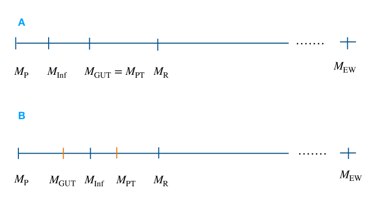
Figure 1: Possible scenarios for the completion of the phase transition. In scenario “A”, the phase transition happens at the scale of grand unification and after the inflation scale, so its effects are visible today. Scenario “B” refers to the case that the phase transition does not complete at $M_{\text{GUT}}$ but is completed after inflation. We briefly mention this possibility in Section 4.

To conclude this section, we mention that a supersymmetric version of this model, breaking supersymmetry at a high scale could be realized with a modification of the breaking chain as

$$SO(10) \xrightarrow[45~[\mbox{\scriptsize{1}]}]{M_{\text{GUT}}} SU(3)_{C}\times SU(2)_{L}\times SU(2)_{R}\times U(1)_{B-L}$$

$$\xrightarrow[~[\mbox{\scriptsize{1}]}]{M_{R}} SU(3)_{C}\times SU(2)_{L}\times U(1)_{R}\times U(1)_{B-L}$$

$$\xrightarrow[126~[\mbox{\scriptsize{2}]}]{M_{R}} SU(3)_{C}\times SU(2)_{L}\times U(1)_{Y}\times\mathbb{Z}_{2}\xrightarrow[10]{\>M_{\text{EW}}}SU(3)_{C}\times U(1)_{\text{em}}\times\mathbb{Z}_{2}\,.$$

The construction of the potential that could lead to a phase transition is different from the case we discuss here, and we will leave it for future work. It is worth mentioning that for this case the cosmic strings generated at the scale $M_{R}$ can trigger on their own the monopole decay.

2.2 Definition and Matter Content

We consider the minimal $SO(10)$ model containing only the gauge bosons, the three families of fermions transforming under the representation $\mathbf{16}$, as well as scalars transforming under $\mathbf{10}$, $\mathbf{45}$, and $\mathbf{126}$ [15, 16, 17]. We will refer to this model as $\mathbf{G}^{\rm M}_{3221}$, since the first step of symmetry breaking leads to the gauge group

$$G_{3221}:=SU(3)_{C}\times SU(2)_{L}\times SU(2)_{R}\times U(1)_{B-L}\,.$$ (2.4)

We will investigate the potential for a first-order phase transition in this step, triggered by a vev $v$ of the $G_{3221}$-singlet component of the $\mathbf{45}$ (see App. A for details).

As indicated in Eq. (2.1), we assume that a $\mathbf{126}$ vev is solely responsible for the later symmetry breaking to the SM gauge group, which implies that the $SU(2)_{R}$ triplet component of the $\mathbf{45}$ does not obtain a vev, i.e., $\omega_{R}=0$ in the notation of [16, 17]. We also assume that the symmetry breaking does not lead to large mass splittings between particles from the same $SO(10)$ multiplet; thus, all masses of the $\mathbf{45}$ scalars are of $\mathcal{O}(M_{\text{GUT}})$ and all masses of the $\mathbf{126}$ scalars are of $\mathcal{O}(M_{R})$. The only exception is the multiplet $\mathbf{10}$, where a large splitting is required between the doublet and triplet components to avoid rapid proton decay, of course, cf. Section 2.5.2. Finally, we assume that one doublet component of the $\mathbf{10}$ obtains a mass of $\mathcal{O}(M_{R})$. In other words, below $M_{R}$ we have exactly the gauge group and particle content of the SM.

2.3 Effective Potential

In this section, we present the main results for the contributions to the effective scalar potential, including $1$-loop and thermal corrections. Details of the computation are given in App. B. We start with the tree-level $SO(10)$-symmetric potential for the scalar $\mathbf{45}$,

$$V_{0}(\phi)=-\frac{\mu^{2}}{2}\operatorname{Tr}\phi^{2}+\frac{a_{0}}{4}\left(\operatorname{Tr}\phi^{2}\right)^{2}+\frac{a_{2}}{4}\operatorname{Tr}\phi^{4}$$ (2.5)

with $\mu^{2}>0$. In terms of the classical field $\phi_{c}$, the tree-level potential corresponding to the chain in Eq. (2.4), is obtained by plugging Eq. (B.1) into Eq. (2.5), resulting in

$$V_{0}(\phi_{c})=-\frac{1}{2}\mu^{2}\varphi_{c}^{2}+a_{0}\varphi_{c}^{4}+\frac{1}{6}a_{2}\varphi_{c}^{4}\,.$$ (2.6)

Defining the unification scale $v\equiv M_{\text{GUT}}$ as the value of the classical field $\varphi_{c}$ at the potential minimum, the tree-level minimization condition yields

$$\mu^{2}=\Bigl{(}4a_{0}+\frac{2}{3}a_{2}\Bigr{)}\,v^{2}\,.$$ (2.7)

The $1$-loop contribution to the effective potential at zero temperature, $V_{1}(\phi_{c})$, contains two parts, the gauge boson contribution

$$V_{1}^{g}(\phi_{c})=\frac{3}{64\pi^{2}}\sum_{i=g1,g2}n_{i}\,m_{i}^{4}(\phi_{c})\left(\ln\frac{m_{i}^{2}(\phi_{c})}{\mu_{r}^{2}}-\frac{5}{6}\right),$$ (2.8)

and the scalar contribution

$$V_{1}^{s}(\phi_{c})=\frac{1}{64\pi^{2}}\sum_{i=s1,s2,s3,\chi}n_{i}\,m_{i}^{4}(\phi_{c})\left(\ln\frac{|m_{i}^{2}(\phi_{c})|}{\mu_{r}^{2}}-\frac{3}{2}\right),$$ (2.9)

where $m_{i}(\phi_{c})$ is the field-dependent mass of the gauge boson or scalar $i$ and $n_{i}$ the number of particles with this mass. Both quantities are given in Tab. 1. These expressions have been obtained in the $\overline{\text{MS}}$ renormalization scheme with the renormalization scale $\mu_{r}$, for which we choose $\mu_{r}=v$ in numerical calculations. Note that the scalar contribution contains both the physical scalars and the Nambu-Goldstone bosons. As the masses of the scalars from representations other than $\mathbf{45}$ are significantly smaller than $v$, the same holds for their field-dependent masses, and thus it is safe to assume that their contributions to the effective potential have a negligible impact on the phase transition. Note that the scalar potential that we are considering here for the first step of the symmetry breaking is independent of any physics below the unification scale, of course apart from the value of the unification scale, which is determined by the breaking chain and the matter content.

Field-dependent mass squared		Particle type	Multiplicity $n_{i}$
$m_{g1}^{2}(\phi_{c})$	$\frac{1}{6}g^{2}\varphi_{c}^{2}$	Gauge boson	$24$
$m_{g2}^{2}(\phi_{c})$	$\frac{2}{3}g^{2}\varphi_{c}^{2}$	Gauge boson	$6$
$m_{s1}^{2}(\phi_{c})$	$-\mu^{2}+4a_{0}\varphi_{c}^{2}$	Scalar	$6$
$m_{s2}^{2}(\phi_{c})$	$-\mu^{2}+12a_{0}\varphi_{c}^{2}+2a_{2}\varphi_{c}^{2}$	Scalar	$1$
$m_{s3}^{2}(\phi_{c})$	$-\mu^{2}+4a_{0}\varphi_{c}^{2}+2a_{2}\varphi_{c}^{2}$	Scalar	$8$
$m_{\chi}^{2}(\phi_{c})$	$-\mu^{2}+4a_{0}\varphi_{c}^{2}+\frac{2}{3}a_{2}\varphi_{c}^{2}$	NGB	$30$

Table 1: Field-dependent masses. The multiplicity indicates the number of particles with this mass.

In Eq. (B.6) we specify the $1$-loop contributions to the effective potential at finite temperature, $V_{\rm{th}}(\phi_{c},T)$. Then the complete $1$-loop effective potential is given by

$$V(\phi_{c},T)=V_{0}(\phi_{c})+V_{1}^{g}(\phi_{c})+V_{1}^{s}(\phi_{c})+V_{\text{th}}(\phi_{c},T)\,.$$ (2.10)

We need to find the minimum of the potential including these corrections. The condition for the minimum at zero temperature is

$$\frac{\partial V(\phi_{c},0)}{\partial\phi_{c}}=\frac{\partial V_{0}(\phi_{c})}{\partial\phi_{c}}+\frac{\partial V_{1}^{g}(\phi_{c})}{\partial\phi_{c}}+\frac{\partial V_{1}^{s}(\phi_{c})}{\partial\phi_{c}}=0,$$ (2.11)

which can be solved numerically. What we adopt here is a similar strategy to the one followed in [16] in that we adjust the value of $\mu^{2}$ such that the minimum at the $1$-loop level is roughly equal to $v$. We remind the reader that $v$ is fixed by the gauge coupling unification condition, as we will discuss in Section 2.4. Specifically, we calculate $\mu^{2}$ at the tree level from Eq. (2.7) and use it in Eq. (2.11) to find the value of the scalar field in the minimum, denoted by $\phi_{m}$. This value differs from $v$, so we update $\mu^{2}$ iteratively using Newton’s method until $\phi_{m}$ differs from $v$ by no more than $1\,\%$. As the value of $\mu^{2}$ thus obtained approaches zero, the calculation becomes numerically challenging due to convergence issues and large higher-order loop corrections. Therefore, we exclude points with $\mu^{2}<0$.

Given the size of the gauge coupling at the GUT scale (around $0.5$ as we explain in Section 2.4) and the particle content of the model (thirty massive gauge bosons and fifteen scalar bosons), we expect that loop corrections can become big and one-loop precision may not be sufficient. As a two-loop computation is beyond the scope of this work, we adopt the usual strategy for estimating the uncertainty caused by neglecting higher loop orders, see e.g. [25, 26], defining the quantity

$$\Delta^{\text{2-loop}}:=\left\langle\frac{\left.V(\phi_{c},0)\right|_{\mu_{r}=2v}-\left.V(\phi_{c},0)\right|_{\mu_{r}=v/2}}{\big{(}\left.V(\phi_{c},0)\right|_{\mu_{r}=2v}+\left.V(\phi_{c},0)\right|_{\mu_{r}=v/2}\big{)}/2}\right\rangle_{\!0<\phi_{c}<1.2v}$$ (2.12)

to estimate the importance of higher loop orders, since the exact potential is independent of $\mu_{r}$. The brackets in Eq. (2.12) indicate an average over $1000$ linearly sampled values of $\phi_{c}$ between 0 and $1.2\,v$ to reduce the sensitivity to single points in field space where the denominator becomes very small due to cancellations.

Before presenting the parameter space where a first-order phase transition would be possible, we discuss in the next sections constraints on the model that lead to bounds on the unification scale and on the parameter space of the coefficients in the potential.

2.4 Gauge Coupling Running

The minimal version of the model with the breaking chain of Eq. (2.1) contains the scalar $\mathbf{45}$ which breaks the $SO(10)$ group, then the ${\mathbf{126}}$ breaks subsequently to $G_{SM}$ and then the $\mathbf{10}$ causes the breaking at the electroweak (EW) scale. Our convention for the order of the indices is $a=3,2L,2R,B-L$ for this model the component acquiring a vev in the $\mathbf{126}$ is $(1,1,3,2)$ and that of $\mathbf{10}$ is $(1,2,2,0)$ $\supset(2,1,\pm 1/2)$. Where this last decomposition is under the SM group, $SU(2)_{L}\times SU(3)_{C}\times U(1)_{Y}$. For the matter, we have the three families of fermions: $(3,2,1,-1/3)$, $(1,2,1,1)$, $(\overline{3},1,2,1/3)$ and $(1,1,2,-1)$. However, we just take into account the running of the top mass up to the $M_{R}$ scale. With this minimal matter content, the beta function coefficients at one and two loops are, respectively [27, 28, 8],

$$b_{a}^{(1)}=\left(\begin{array}[]{c}-7\\ -3\\ -7/3\\ 11/2\\ \end{array}\right),\quad b_{ab}^{(2)}=\left(\begin{array}[]{cccc}-26&9/2&9/2&1/2\\ 12&8&3&3/2\\ 12&3&80/3&27/2\\ 12&9/2&81/3&61/2\\ \end{array}\right).$$ (2.21)

The matching conditions at the scale $M_{R}$ are

$$g^{SM}_{2}(M_{R}) = g^{G_{3221}}_{2L}(M_{R})\,,$$

$$g^{SM}_{1}(M_{R}) = \left[\frac{3}{5}\frac{1}{{g^{G_{3221}}_{2R}}^{2}(M_{R})}+\frac{2}{5}\frac{1}{{g^{G_{3221}}_{B-L}}^{2}(M_{R})}\right]^{-1/2},$$

$$g^{SM}_{3}(M_{R}) = g^{G_{3221}}_{3}(M_{R})\,,$$ (2.22)

where $g^{G_{3221}}_{2L}$, $g^{G_{3221}}_{2R}$ $g^{G_{3221}}_{B-L}$ and $g^{G_{3221}}_{3}$ are respectively the couplings of the group factors $SU(2)_{L}$, $SU(2)_{R}$, $U(1)_{B-L}$ and $SU(3)_{C}$. To unclutter the notation, from now on we suppress the superscript $G_{3221}$.

When running up the SM gauge coupling and matching to the $G_{3221}$ group we need to make a guess about the relation between $g_{2R}$ and $g_{2L}$ but after running back and forth, in the final run from $M_{\text{GUT}}$ to $M_{R}$, we can then obtain the final predicted value for $g_{2R}(M_{R})$ and $g_{2L}(M_{R})$. The beta functions take the form $dg_{a}/dt=g_{a}^{3}b_{a}/16\pi^{2}+g_{a}^{3}/(16\pi^{2})^{2}\left[\sum_{b=1}^{4}b_{ab}g_{b}^{2}\right]$, for $a=3,2L,2R,B-L$ and the coefficients $b_{a}$ and $b_{ab}$ as in Eq. (2.21). For the SM, $dg_{a}/dt=g_{a}^{3}b_{a}/16\pi^{2}+g_{a}^{3}/(16\pi^{2})^{2}\left[\sum_{b=1}^{3}b_{ab}g_{b}^{2}-C_{a}^{t}y_{t}^{2}\right]$ with $C_{1}=17/10$, $C_{2}=3/2$, $C_{3}=2$, for $a=1,2,3$ representing respectively the SM group factors $U(1)_{Y},SU(2)_{L},SU(3)_{C}$. The coefficients $b_{a}$ and $b_{ab}$ for this case are very well known and can be found in [29]. Just with this minimal content the scales are

$$M_{R}^{2\,\rm{loop}} = (2.9\pm 1.0)\times 10^{9}\,\text{GeV}\,,$$

$$M_{\text{GUT}}^{2\,\rm{loop}} = (1.60\pm 1.0)\times 10^{16}\,\text{GeV}\,.$$ (2.23)

Once various thresholds are considered, at two-loop precision the scale $M_{\text{GUT}}$ can drop to $\mathcal{O}(10^{15})\,\text{GeV}$ [17] for the minimal setting. However, finding all phenomenology to be viable, especially in the Higgs sector at the EW scale [17], seems challenging. Adding matter content impacts the running and so the unification scale. Therefore, in what we consider here we set values of the unification scale in the range from $10^{15}\,\text{GeV}$ to $1.6\times 10^{16}\,\text{GeV}$.

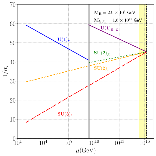
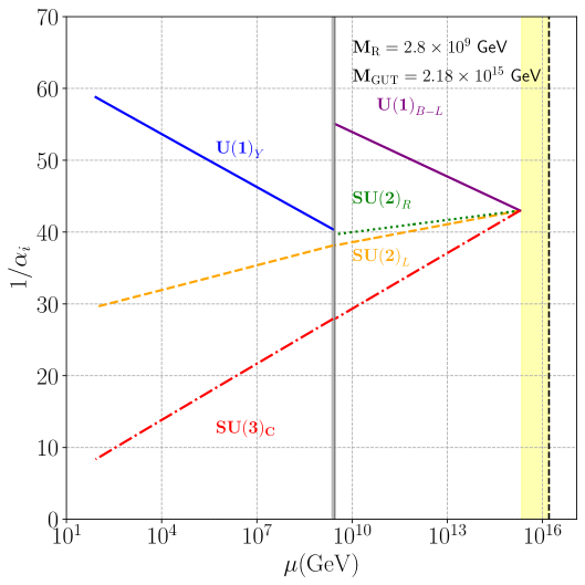
Figure 2: The left panel represents the running of the Minimal $\mathbf{G}_{3221}$ model: $\mathbf{G}^{\rm M}_{3221}$ (containing only $\mathbf{45}\oplus\mathbf{126}\oplus\mathbf{10}$), with $M_{R}=(2.9\pm 1.0)\times 10^{9}\,\text{GeV}$ and $M_{\text{GUT}}=(1.60\pm 1.0)\times 10^{16}\,\text{GeV}$. The gauge couplings of the groups of the SM are run up to $M_{R}$ and those of $SU(3)_{C}\times SU(2)_{L}\times SU(2)_{R}\times U(1)_{B-L}$ from $M_{R}$ and $M_{\text{GUT}}$. The vertical gray band around $2.8\times 10^{9}$ GeV represents the band for $M_{R}$ allowed for $M_{R}$ for this model and the model of the right plot. The right plot represents the running of the $\mathbf{G}_{3221}$ model plus a scalar Dark Matter $SU(2)_{R}$-$SU(2)_{L}$ bi-doublet candidate (that of the third panel Fig. 9 of [30]). We present this last plot as an example that the addition of matter can alter the running (see Eq. (2.24) and the text below) of the gauge coupling constants and reduce the unification scale.

Since it is challenging to accommodate the EW physics in the minimal $G^{\rm M}_{3221}$, we may consider the addition of more scalars or fermions. For this purpose, we recall the general expression for the 1-loop beta function

$$\beta_{g_{i}}=\frac{g^{3}}{16\pi^{2}}b_{i},\quad b_{i}=\left[-\frac{11}{3}C(G_{i})+\frac{2}{3}\sum S(R_{F_{i}})+\frac{1}{3}\sum S(R_{S_{i}})\right],$$ (2.24)

for $F_{i}$ chiral fermions and $S_{i}$ real scalars. As it is well known, for the SM $SU(3)_{C}$ factor, we have $C(SU(3)_{C})=3$, and $S(R_{F_{i}})=6$, rendering the famous $b_{3}=-7$. We can see that the addition of particles that make $b_{3}$ less negative, for example, colour triplets, flattens the running of $1/\alpha_{3}$ and shifts $M_{\text{GUT}}$ to higher scales and $M_{R}$ to lower scales. But as some of us noted in [30], the addition of colour triplets is not enough because multiplets of all the other groups are required in order to ensure that the couplings $g_{2L}$ and $g_{2R}$ unify at high scale. As an example, in Fig. 2 we plot the running of the gauge couplings when a Dark Matter scalar candidate has been added to the running of the model $G_{3221}$ with an additional scalar which is both doublet of $SU(2)_{R}$ and $SU(2)_{L}$ (referred to as “bi-doublet”) and singlet of $SU(3)_{C}$. For this case the GUT scale is located at $2.8\times 10^{15}\,\text{GeV}$. Further examples of adding Dark Matter candidates can be found in [27, 30]. Note that in our analysis of FOPT, we consider both the maximum scale $M_{\text{GUT}}=1.6\times 10^{16}\,\text{GeV}$ and the scale $M_{\text{GUT}}=10^{15}\,\text{GeV}$ because that scale is still compatible with proton decay. One further justification for this is that we can add matter at lower energies, that will alter the scale of gauge coupling unification but not the basic characteristics of the potential of Eq. (2.5).

2.5 Constraints within the Model

2.5.1 Mass Spectrum

Calculating the mass spectrum arising from the GUT-scale symmetry breaking step, one encounters particles with negative mass-squared, i.e., tachyons. However, taking into account loop corrections to the masses, it turns out that this problem can be avoided if the quartic couplings of the scalar $\mathbf{45}$ are restricted to [16]

$$a_{0}\in(0.0,0.2)\quad,\quad a_{2}\in(-0.05,-0.01)\,.$$ (2.25)

Hence, we will only consider parameter values within these ranges in our analysis.

2.5.2 Proton Decay

Here we follow [27, 31, 8] and give a brief account on the way proton decay rates are calculated. The most sensitive channel for non-superysmmetric models is the dimension-6 operator induced decay $p\rightarrow\pi^{0}\,e^{+}$ which is mediated by gauge fields. The proton decay for this channel can be estimated as [27]

$$\Gamma(p\rightarrow\pi^{0}\,e^{+}) = \frac{m_{p}}{32\pi}\left(1-\frac{m^{2}_{\pi^{0}}}{m^{2}_{p}}\right)^{2}\,\left[|\mathcal{A}_{L}(p\rightarrow\,\pi^{0}\,e^{+})|^{2}+|\mathcal{A}_{R}(p\rightarrow\,\pi^{0}\,e^{+})|^{2}\right],$$ (2.26)

where $m_{p}$ and $m_{\pi^{0}}$ are respectively the proton and the neutral pion masses. The amplitudes at the weak scale are given by

$${\mathcal{A}_{L}}(p\rightarrow\pi^{0}\,e^{+}) = C_{RL}((ud)_{R}u_{L})(\mu=2\,\rm GeV)\langle{\it{\pi}}^{0}{\it{|(ud)_{R}u_{R}|p}}\rangle,$$

$${\mathcal{A}_{R}}(p\rightarrow\pi^{0}\,e^{+}) = 2C_{LR}((ud)_{L}u_{R})(\mu=2\,\rm GeV)\langle{\it{\pi}}^{0}{\it{|(ud)_{R}u_{R}|p}}\rangle,$$ (2.27)

where the Wilson coefficients $C_{RL}((ud)_{R}u_{L})$ and $C_{LR}((ud)_{L}u_{R})$ correspond respectively to $C_{1}$ and $C_{2}$ of [27]. For numerical values we use the inputs given in Tab. 1 in [8], including the value of the hadronic matrix elements and the evolution of the Wilson coefficients from $M_{\text{GUT}}$ is given in [31]. For the minimal $G_{3221}$ model, we obtain $(2.4\pm 1.6)\times 10^{36}$ years, a safe value given the current experimental bound of $\tau(p\rightarrow\phi^{0}e^{+})>1.6\times 10^{34}$ years at 95% C.L. [32] and the projected bound of $7.8\times 10^{34}$ years at 95% C.L. [33].

3 Appearance of a First Order Phase Transition

3.1 Preliminaries

In this section, we briefly mention only the salient concepts pertaining FOPT, which have been studied extensively (see for example [34]), in order to explain our results. As it is well known, FOPT can generate GW through nucleation, expansion, collision, and merger of bubbles in the broken phase. In vacuum, GW originate solely from bubble collisions and can be described by the envelope approximation [35]. In a thermal plasma, however, friction slows bubble expansion, transferring most of the energy to the plasma and making scalar field contributions subdominant. Lattice simulations show that this energy drives sound waves in the plasma, leading to an acoustic phase that dominates GW production [36, 37]. For stronger transitions, turbulence may emerge, sustaining GW emission until it dissipates [38, 39, 40, 41, 42]. To model these effects, we use GW templates from 3D simulations that fit the spectrum in terms of phase transition parameters and frequency [43, 44, 45]. Key quantities characterizing the GW are $\alpha$ and $\beta$, respectively, the ratio of released vacuum energy to the plasma’s radiation energy in the symmetric phase and a measure of the duration of the phase transition. For completeness, the formulas that we use for $\alpha$ and $\beta$ are presented in Eq. (C.2) and Eq. (C.3), while the 3D action, $S_{3}$, describing the bubbles forming when the transition between the meta-stable and the ture vacuum takes place is given in Eq. (C.1). According to [46, 47, 48] the decay rate, $\Gamma(T)$, of a bubble is given by

$$\Gamma(T)\simeq\max\left[T^{4}\left(\frac{S_{3}}{2\pi T}\right)^{\frac{3}{2}}\exp\left(-S_{3}/T\right)\,,\,R_{0}^{-4}\left(S_{4}/2\pi\right)^{2}\exp(-S_{4})\right].$$ (3.1)

Taking the first expression to be valid we can calculate the nucleation temperature $T_{n}$, at which the average number of bubbles nucleated per Hubble horizon is of order 1:

$$N(T_{n})=\left(\frac{3\overline{M}_{\text{Pl}}}{\pi}\right)^{4}\left(\frac{10}{g_{*}}\right)^{2}\int_{T_{n}}^{T_{c}}\frac{dT}{T^{5}}\left(\frac{S_{3}}{2\pi T}\right)^{3/2}\exp{(-S_{3}/T)}\sim 1\,,$$ (3.2)

which is equivalent to computing the nucleation temperature by taking $\Gamma/V$, where $V$ is the comoving volume, as

$$\frac{\Gamma}{V}\approx T_{n}^{4}e^{S_{3}(T_{n})/T_{n}}\,,$$ (3.3)

integrating to the time $t_{*}$ at which the phase transition takes place and requiring that the total number of bubbles nucleated from time $t=0$ to $t=t_{*}$ is of order 1. Eq. (3.3) has no solution when

$$\frac{\Gamma}{V}<H^{4}\,,$$ (3.4)

which can be written as

$$\frac{S_{3}(T)}{T}>4\log\left(\frac{\overline{M}_{\text{Pl}}}{T}\right)-2\log\left(\frac{90}{\pi^{2}g_{*}(T)}\right).$$ (3.5)

In this case the transition is not completed. For finding the suitable parameter space where a FOPT may occur, we consider the one-loop corrected potential with thermal corrections in Eq. (2.10) and the criterion Eq. (3.2) to determine whether nucleation is possible. We note that for the potential that we are considering, the temperature correction always grows and has a different sign with respect to the tree-level and 1-loop contributions, which need to have a minimum and become negative. In this regard, the thermal contribution is typically necessary to produce a barrier. As is well understood, a barrier can occur if there is a cubic term in the field in the 1-loop thermally corrected potential (where the total contribution to the potential is $\phi^{3}E$, where $E$ has mass dimension $1$ and could be temperature-independent). $E$ is proportional to $g^{3}$ and hence the appearance of a barrier enhances with $g^{3}$.

Above the unification scale, the considered model contains $96$ fermionic ($3$ generations in the representation $\mathbf{16}$, $2$ possible spin orientations) and $307$ scalar degrees of freedom ($45$ massless gauge bosons, $10+45+126\times 2$ real scalars), which yields $g_{*}=481$ effective relativistic degrees of freedom. However, nucleation happens at temperatures below $M_{\text{GUT}}$, where some of the particles obtaining GUT-scale masses are non-relativistic. To account for this, we use $g_{*}=300$ in our computations.

3.2 Results

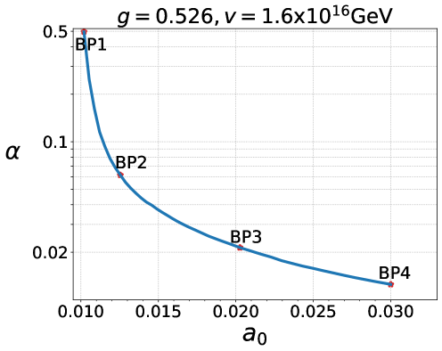
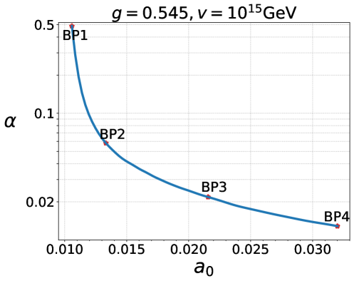
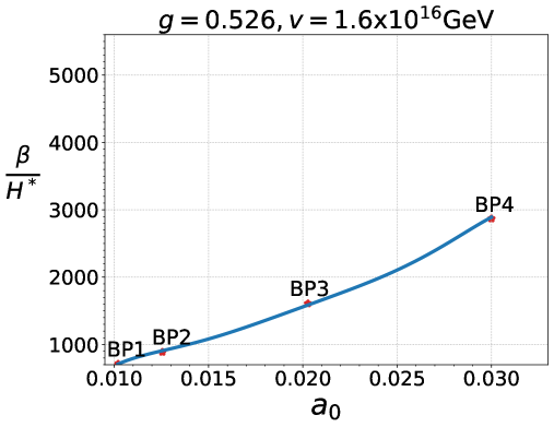
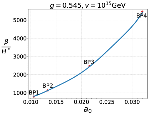
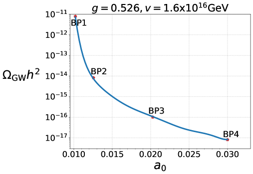
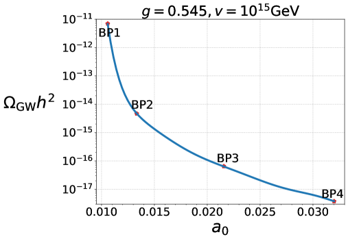
Figure 3: Phase transition parameters ($\alpha$, $\beta/H_{*}$) and GW density as a function of $a_{0}$ for the scales $M_{\text{GUT}}=1.6\times 10^{16}\,$GeV, left, and $M_{\text{GUT}}=1.0\times 10^{15}\,$GeV, right. The (red) dots represent the benchmark points listed in Tables 2 and 3.

We start by discussing the behaviour of the phase transition parameters $\alpha$ and $\beta/H_{*}$, which indicate the strength and the inverse duration, respectively, see Appendix C. In Fig. 3 we collect the results for the scales $M_{\text{GUT}}=1.6\times 10^{16}\,\text{GeV}$ and $M_{\text{GUT}}=1.0\times 10^{15}\,\text{GeV}$. As is known, $\alpha$ and $\beta/H_{*}$ are not completely independent parameters, since both of them depend on the 3D action, Eq. (C.1) and they have opposite behaviours, that is, when $\alpha$ increases, $\beta/H_{*}$ decreases. This behaviour can be clearly seen in Fig. 3, where we plot $\alpha$ and $\beta$ as a function of the parameter $a_{0}$, Eq. (2.6), and whose range is constrained, such as to avoid a tachyonic spectrum, Eq. (2.25). We have also marked four representative benchmark points (BP) and we give the critical, nucleation temperature, $\alpha$ and $\beta$ in Tab. 2. In addition, in Fig. 3, we have plotted the GW energy density as computed with the equations of Appendix C. Since $\Omega_{\text{GW}}h^{2}$ is proportional to $\alpha^{2}/(\beta/H_{*})$, $\Omega_{GW}h^{2}$ follows a decreasing behaviour as $a_{0}$ grows, just as in the case of $\alpha(a_{0})$. For each point in $a_{0}$, $\mu^{2}$ and $a_{2}$ are computed following the algorithm described in Section 2.3.

In order to see the behaviour of the observable $\Omega_{\text{GW}}h^{2}$ as a function of both parameters $a_{0}$ and $a_{2}$, we present Fig. 4 and Fig. 5 for $M_{\text{GUT}}=1.6\times 10^{16}\,\text{GeV}$ and $M_{\text{GUT}}=1.0\times 10^{15}\,\text{GeV}$, respectively. We have also marked the four benchmark points (BP) as well as the lines corresponding to the parameter values for which the curves in Fig. 3 have been computed. We show in solid gray the part of the allowed parameter space of $a_{0}$ and $a_{2}$ that allows for a first-order phase transition. The shading indicates the order of magnitude of the GW signal, with lighter shading corresponding to a stronger signal. Inside the yellow region indicated by “No nucleation”, there is no potential barrier and nucleation is not possible. Its exact boundary is difficult to determine because close to it the numerical algorithm eventually fails when $T_{0}\rightarrow T_{c}$.

We see that the borders of the shaded regions are nearly parallel. Hence, the signal strength does not depend on $a_{0}$ and $a_{2}$ separately, but to a good approximation only on a linear combination. Consequently, the two-dimensional plots in Fig. 3 are sufficient to encode most of the parameter dependence, as a parallel shift of the line connecting the benchmark points would lead to curves very similar to those in Fig. 3.

The hatched regions mark parameter space points where $\Delta^{\text{2-loop}}$ of Eq. (2.12) is larger than $0.5$, indicating that the precision of our one-loop calculation is likely to be insufficient. As the GW signal is strongest in these regions, extending the calculation to include higher loop orders would be a highly desirable goal for future work. We see that BP2 is at the border of the region with $\Delta^{\text{2-loop}}>0.5$ and thus corresponds to the largest signal strength for which we are confident in the accuracy of our calculation. In contrast, BP1 has the largest value of $\Delta^{\text{2-loop}}$ and should therefore be regarded with caution.

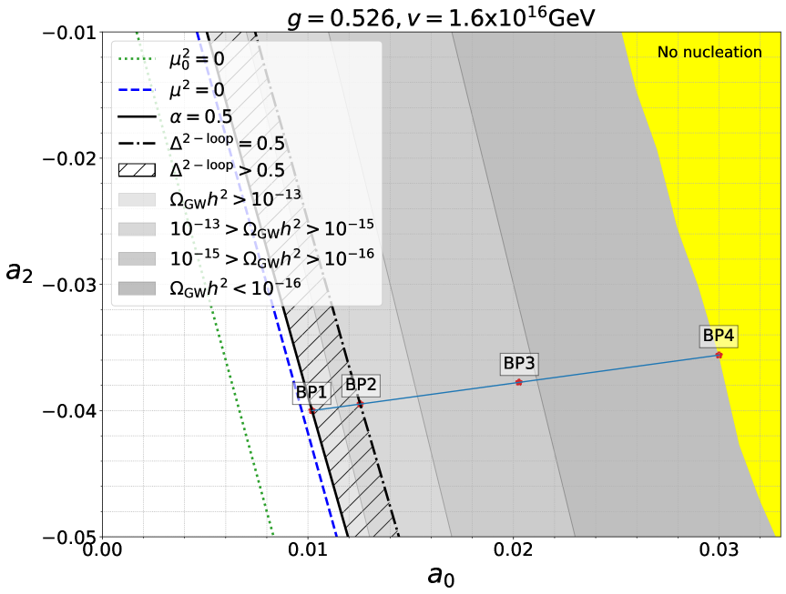
Figure 4: GW parameter space for $a_{0}$ vs. $a_{2}$, where $a_{2}$ is restricted to the region where the spectrum does not contain tachyons. The four points marked by stars are our benchmark points. The yellow region has no FOPT or is numerically difficult to calculate. In the hatched region, $\Delta^{\text{2-loop}}>0.5$. We denote the quadratic term in the scalar potential obtained from the tree-level condition (2.7) by $\mu_{0}^{2}$. In contrast, $\mu^{2}$ is the corrected value of this parameter ensuring that the $1$-loop-corrected scalar potential has a minimum at $v$.

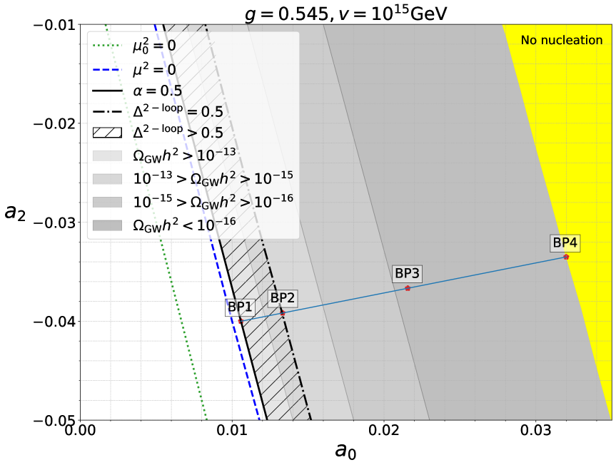
Figure 5: The same as in Fig. 4 but for $M_{\text{GUT}}=1.0\times 10^{15}\,\text{GeV}$.

The plots also include the lines on which the quadratic term in the scalar potential vanishes at tree level ($\mu_{0}^{2}=0$, by which we mean that the r.h.s. of Eq. (2.7) vanishes) and at the one-loop level ($\mu^{2}=0$, cf. the discussion in Section 2.3). Evidently, a strong signal corresponds to small values of $\mu^{2}$.

BP	$T_{0}/M_{\text{GUT}}$	$T_{c}/M_{\text{GUT}}$	$T_{n}/M_{\text{GUT}}$	$\alpha$	$\beta/H_{*}$	$a_{0}$	$a_{2}$
BP1	0.0603	0.119	0.0638	0.50	$7.1\times 10^{2}$	0.0102	$-0.04$
BP2	0.136	0.170	0.142	0.062	$8.9\times 10^{2}$	0.0125	$-0.0394$
BP3	0.242	0.259	0.249	0.021	$1.6\times 10^{3}$	0.0202	$-0.0377$
BP4	0.308	0.318	0.313	0.013	$2.9\times 10^{3}$	0.03	$-0.0356$

Table 2: Phase transition parameters for four benchmark points with $M_{\text{GUT}}=1.6\times 10^{16}\,$GeV.

BP	$T_{0}/M_{\text{GUT}}$	$T_{c}/M_{\text{GUT}}$	$T_{n}/M_{\text{GUT}}$	$\alpha$	$\beta/H_{*}$	$a_{0}$	$a_{2}$
BP1	0.0603	0.122	0.0659	0.49	$7.9\times 10^{2}$	0.01058	$-0.04$
BP2	0.141	0.176	0.150	0.058	$1.1\times 10^{3}$	0.0133	$-0.0391$
BP3	0.244	0.261	0.252	0.022	$2.5\times 10^{3}$	0.0215	$-0.0366$
BP4	0.309	0.319	0.316	0.013	$5.5\times 10^{3}$	0.032	$-0.0335$

Table 3: Phase transition parameters for four benchmark points with $M_{\text{GUT}}=1.0\times 10^{15}\,$GeV.

4 Incomplete Phase Transitions

In Section 3.2, we have seen that for both cases of $M_{\text{GUT}}=1.6\times 10^{16}\,\text{GeV}$ and $M_{\text{GUT}}=1.0\times 10^{15}\,\text{GeV}$, there is a parameter space in $a_{0}$ and $a_{2}$ (see the yellow region of Fig. 4 and Fig. 5) where the phase transition does not complete at the GUT scale. For these cases, we could have the scenario “B”, depicted in Fig. 1, because the criterion of Eq. (3.5) is satisfied. As pointed out in [13], the phase transition can still occur at a lower scale, leaving an imprint in the CMB. For this to happen the scalar field breaking the GUT theory needs to act like a spectator value during inflation, Eq. (3.4) has to be satisfied and $V_{\rm Inf}(\phi_{\rm Inf})\gg V(\phi)$, where we have called $\phi_{\rm Inf}$ the field triggering inflation. What is relevant for the breaking chain that we are considering is that the scalar spectrum is modified and the induced GW can be seen at lower frequencies than those of the phase transitions and the plasma. This depends on the phase transition parameters and is governed by the dimensionless parameter $\gamma_{PT}:=1/H^{4}\,\Gamma/V\big{(}\Delta V(\phi)/\dot{\phi}_{\rm Inf}\big{)}^{2}$, defined in [13]. In the yellow region of Fig. 4 and Fig. 5, $1/H^{4}\,\Gamma/V<1$ and we can compute it in those regions. The other term in $\gamma_{PT}$ depends on details of inflation and since we do not have a model of inflation we can give an upper bound $\gamma_{PT}\leq 10^{-3}\big{(}\Delta V(\phi)/\dot{\phi}_{\rm Inf}\big{)}^{2}$, since the scale of $V(\phi)\ll V_{\rm Inf}(\phi_{\rm Inf})$ we expect that $V(\phi)\ll V_{\rm Inf}(\phi_{\rm Inf})\ll 1$ at the end of inflation when the slow-roll parameter is close to unity. For illustration, we plot in Fig. 8 the region in the plane of frequency vs. $\Omega_{\text{GW}}h^{2}$ at which these signals could potentially be observed.

5 Gravitational Waves from the SO(10) Plasma

Any plasma in thermal equilibrium emits GW [49]. The signal is determined by the shear viscosity of the plasma. In the SM it is a certainty that it is present, but the ultra-high frequency of the GW makes them challenging to discover. Scenarios of physics beyond the SM can both lower the peak frequency and enhance the signal as a result ofesult of the many additional degrees of freedom. As the shear viscosity changes during the different stages of the GUT symmetry breaking down to the SM, we obtain a different signal during each particular stage. Furthermore and more importantly, as the breaking scales $M_{\text{GUT}}$ and $M_{R}$ are fixed by gauge coupling unification, the maximum temperature of each stage is fixed, unlike the SM, where the maximum temperature is the reheating temperature and thus a free parameter. In the following, we determine the GW signal for each breaking stage, following [49, 50].

In this work, we present the results for the GW signal from the plasma during the three steps of symmetry breaking shown in Eq. (2.1) with the minimal content of matter. For each step, we take Eq. (5.6) and use the well-known expression for the GW produced by a plasma in equilibrium [49],

$$\Omega_{\text{GW}}(f,T_{0})\,h^{2}=\Omega_{\gamma_{0}}h^{2}\frac{\lambda}{\overline{M}_{\text{Pl}}}\int^{T_{\rm Max}}_{T_{\rm EWCO}}\,dT\left(\frac{g_{*0}}{g_{*}(T)}\right)^{4/3}\,T^{2}\,\hat{k}(f,T)^{3}\frac{\eta(\hat{k},T)}{\sqrt{\rho(T)}}\,\beta(T)\,,$$ (5.1)

where $\Omega_{\rm{GW}}(f,T_{0})$ is the fraction of energy released into GW radiation per frequency octave [1], $\lambda=30\sqrt{3}/\pi^{4}$ and

$$\hat{k}(f,T):=\frac{k}{T}=\left[\frac{g_{*s}(T)}{g_{*s}(T_{0})}\right]^{\frac{1}{3}}\frac{2\pi f}{T_{0}},\quad f=\frac{1}{2\pi}\left[\frac{g_{\rm*s}(T_{0})}{g_{\rm*s}(T_{\rm EWCO})}\right]^{\frac{1}{3}}\left(\frac{T_{0}}{T_{\rm EWCO}}\right)k_{\rm EWCO}\,.$$ (5.2)

In these equations, $T_{\rm EWCO}=160\,\text{GeV}$,

$$k_{\rm EWCO}=k(T)\left(g_{*s}(T_{\rm EWCO})/g_{*s}(T)\right)^{1/3}T_{\rm EWCO}/T$$

is the wave number at $T$ = $T_{\rm EWCO}$, and $T_{\rm Max}$ is the maximum temperature that we identify with the reheating temperature.

The shear viscosity of the SM was computed up to the leading contribution in [49], while accounting for temperature dependence in [50]. For a general theory, we have

$$\eta(\hat{k},T) = \left\{\begin{array}[]{cc}\frac{1}{8\pi}\frac{16}{g_{1}^{4}\ln(5T/m_{D_{1}})},&\,\hat{k}\lesssim\alpha_{1}^{2},\\ \eta_{\rm{HTL}}(\hat{k},T)+\eta^{T}(\hat{k},T),&\hat{k}\gtrsim 3,\end{array}\right.,$$ (5.5)

where $\eta_{\rm{HTL}}$ is the Hard Thermal Logarithmic (HTL) expression [51, 50]

$$\eta_{\text{HTL}}(\hat{k},T)=\frac{1}{16\pi}\hat{k}n_{B}(\hat{k})\,\sum^{m}_{n=1}d_{n}{\hat{m}}^{2}_{D_{\mathcal{G}_{n}}}\ln\left(4\frac{{\hat{k}}^{2}}{\hat{m}^{2}_{D_{\mathcal{G}_{n}}}}+1\right),$$ (5.6)

where the sum is over the $m$ different groups if the model contains more than one group factor, $d_{n}$ is the number of generators of the given group and the normalized Debye masses are $\hat{m}^{2}_{D_{\mathcal{G}_{n}}}={m}^{2}_{D_{\mathcal{G}_{n}}}/T^{2}$. The $\eta^{T}$ part is a function that depends on the gauge couplings at definite temperature. For the SM, this has been calculated in [50]. In this work, we assume $\eta^{T}\rightarrow 0$ for the SO(10) model but we take into account the value of the gauge couplings at a definite temperature. Note that the first part in Eq. (5.5) corresponds to the hydrodynamic limit (low frequency) and the second term to the leading log (high frequency) [49].

In practice, due to the dominance of $T_{\rm Max}$ and the production of the GW in the radiation era the expression in Eq. (5.1) reduces to

$$\frac{{\Omega_{\rm{GW}}(f,T_{0})h^{2}}}{\Omega_{\gamma_{0}}h^{2}} = \lambda\,\left[\frac{a_{\rm{Max}}T_{\rm{Max}}}{a_{0}T_{0}}\right]^{4}\frac{T_{\rm{EWCO}}-T_{\rm{Max}}}{\overline{M}_{\text{Pl}}}\frac{T^{2}_{\rm{in}}}{\sqrt{\rho}}\,\hat{k}^{3}\,\eta\left(T,\hat{k}\right),$$ (5.7)

which is the expression we use to produce the plots.

We recall that for a general gauge theory the Debye masses of a group factor $\mathcal{G}_{n}$ are given by [52]

$$m^{2}_{D_{\mathcal{G}_{n}}}=g^{2}_{n}T^{2}\left[\frac{1}{3}S(\text{Adj})+\frac{1}{6}\sum_{i}S(R_{F_{i}})+\frac{1}{6}\sum_{j}S(R_{S_{j}})\right],$$ (5.8)

where $S$ is the Dynkin index of a representation (the adjoint representation Adj for the gauge bosons, the $i$-th fermion representation $R_{F_{i}}$, and the $j$-th real scalar representation $R_{S_{j}}$). In our model, the results for the Debye masses, calculated with the help of GroupMath [53], are as follows.

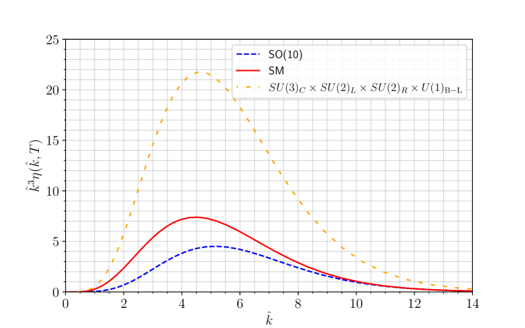
Figure 6: Comparison of the shear viscosity, $\eta$, for the case of the SM, red-solid, and for the SO(10) case, long-dashed and for the group $SU(3)_{C}\times SU(2)_{R}\times SU(2)_{L}\times U(1)_{\rm B-L}$, orange short-dashed.

SO(10) Plasma

For the stage above the unification scale, we have a single group $\mathcal{G}=SO(10)$. There are three families of fermions in the $\mathbf{16}$ representation, that is, $S(\mathbf{16}_{F_{i}})=2$ with $i=1,2,3$. In addition, we have gauge bosons and scalars in the adjoint, $S(\text{Adj})=S(\mathbf{45})=8$, a real scalar multiplet with $S(\mathbf{10})=1$, and complex scalars in the $\mathbf{126}$, so $S(\mathbf{126}_{j})=35$ for $j=1,2$. Summing up these contributions, Eq. (5.8) yields

$$m^{2}_{D_{SO(10)}}=\frac{101}{6}\,g^{2}T^{2}\,,$$ (5.9)

so the contribution to Eq. (5.6) is

$$d_{SO(10)}m^{2}_{D_{SO(10)}}=45\times g^{2}T^{2}\frac{101}{6}\,.$$ (5.10)

$\mathbf{SU(3)}_{C}\times\mathbf{SU(2)}_{L}\times\mathbf{SU(2)}_{R}\times\mathbf{U(1)}_{B-L}$ Plasma

Between the unification scale and the scale of $B-L$ breaking, the plasma contains the fermions, the gauge bosons of the intermediate gauge group $G_{3221}$, the doublet scalars originating from the $\mathbf{10}$, and the scalars from the $\mathbf{126}$. The representations decompose as (for the indices $a=3,2L,2R,B-L$)

$$\mathbf{10} = (\mathbf{1},\mathbf{2},\mathbf{2},0)\oplus\text{(heavy triplets)}\,,$$

$$\mathbf{16} = (\mathbf{3},\mathbf{2},\mathbf{1},\tfrac{1}{3})\oplus(\mathbf{\overline{3}},\mathbf{1},\mathbf{2},-\tfrac{1}{3})\oplus(\mathbf{1},\mathbf{2},\mathbf{1},-1)\oplus(\mathbf{1},\mathbf{1},\mathbf{2},1)\,,$$

$$\mathbf{126} = (\mathbf{\overline{6}},\mathbf{1},\mathbf{3},\tfrac{2}{3})\oplus(\mathbf{\overline{3}},\mathbf{3},\mathbf{1},\tfrac{2}{3})\oplus(\mathbf{\overline{3}},\mathbf{1},\mathbf{1},\tfrac{2}{3})\oplus(\mathbf{8},\mathbf{2},\mathbf{2},0)\oplus(\mathbf{1},\mathbf{2},\mathbf{2},0)\oplus(\mathbf{6},\mathbf{3},\mathbf{1},-\tfrac{2}{3})\oplus$$ (5.11)

$$(\mathbf{3},\mathbf{1},\mathbf{3},-\tfrac{2}{3})\oplus(\mathbf{3},\mathbf{1},\mathbf{1},-\tfrac{2}{3})\oplus(\mathbf{\overline{3}},\mathbf{2},\mathbf{2},-\tfrac{4}{3})\oplus(\mathbf{1},\mathbf{1},\mathbf{3},-2)\oplus(\mathbf{3},\mathbf{2},\mathbf{2},\tfrac{4}{3})\oplus$$

$$(\mathbf{1},\mathbf{3},\mathbf{1},2)$$

in terms of $G_{3221}$ multiplets, where the last number in parentheses indicates $B-L$. Plugging the corresponding $SU(2)$ and $SU(3)$ Dynkin indices as well as $(B-L)^{2}$ into Eq. (5.8), we find

$$d_{i}m^{2}_{D_{i}}=\left\{\begin{array}[]{c}d_{1}\frac{304}{9}g_{B-L}^{2}T^{2},\,d_{1}=1\,,\\ \\ d_{2}\frac{41}{3}g_{SU(2)_{L}}^{2}T^{2},\,d_{2}=3\,,\\ \\ d_{2}\frac{41}{3}g_{SU(2)_{R}}^{2}T^{2},\,d_{2}=3\,,\\ \\ d_{3}\frac{41}{3}g_{3}^{2}T^{2},\,d_{3}=8\,.\end{array}\right.$$ (5.19)

SM Plasma

Below the $B-L$ breaking scale, we have the gauge group and particle content of the SM, so we can use the known results [49]

$$d_{i}m^{2}_{D_{i}}=\left\{\begin{array}[]{c}d_{1}\frac{11}{6}g_{1}^{2}T^{2},\,d_{1}=1\,,\\ \\ d_{2}\frac{11}{6}g_{2}^{2}T^{2},\,d_{2}=3\,,\\ \\ d_{3}2g_{3}^{2}T^{2},\,d_{3}=8\,.\end{array}\right.$$ (5.25)

In Fig. 6 we show the comparison of the shear viscosity, $\eta$ of the SO(10) group, the $G_{3221}$ group and the SM group.

We can see that the peak of the shear viscosity, $\eta$, for the group $G_{3221}$ is enhanced with respect to the SM due to the four group factors, Eq. (5.19), of the $G_{3221}$ model in comparison to the three group factors of the SM model, Eq. (5.25). For this reason, it is clear that the peak of the shear viscosity of the $SO(10)$ group, Eq. (5.10) is further suppressed than that of the SM.

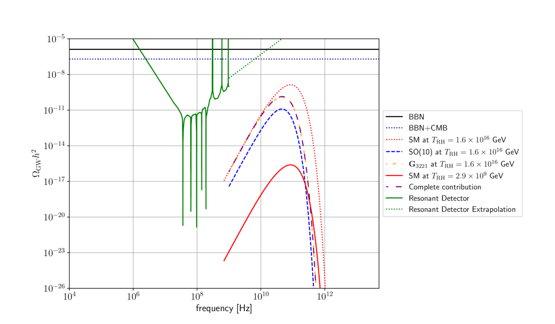
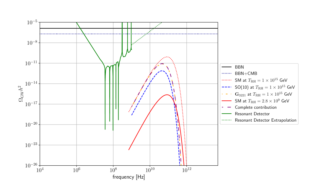
Figure 7: Contributions to GW from plasma fluctuations, shown separately for each step of the breaking chain in Eq. (2.1) for $M_{\text{GUT}}=1.6\times 10^{16}\,\text{GeV}$ (top) and $M_{\text{GUT}}=10^{15}\,\text{GeV}$ (bottom). For comparison, we have also plotted the SM expectation for the same reheating temperature. “Resonant Detector” refers to the proposal in [54]. In this plot we show only the leading-log part in $\eta$, Eq. (5.5), since it is the one that determines the location of the peak. In Fig. 8 we show also the hydrodynamic limit, relevant for disentangling the signal in the low frequency bandwidth from other sources.

Note, however, from Eq. (5.1), that the location of the peak of the density of GW, as a function of the frequency, scales as $(g_{*0}/g_{*}(T))^{4/3}$ and hence the more degrees of freedom the lower the frequency of the peak of the GW density. This is illustrated in Fig. 7 where we have plotted each of the contributions to the GW plasma of the breaking chain of Eq. (2.1). The height of the peak is determined by the maximum attainable temperature at each stage. Note that the $SO(10)$ group would be unbroken from $M_{\text{Pl}}$ down to $M_{\text{GUT}}$ but due to constraints on inflation and thermal equilibrium of the plasma, as mentioned in Section 2, the plasma would enter into thermal equilibrium just close to the GUT scale and therefore we consider the temperature of the $SO(10)$ (dashed blue line) plasma at this temperature. The contribution from $G_{3221}$, short-dashed (orange) line, and the SM contribution, solid red line, which is more than four orders of magnitude suppressed with respect to the $SO(10)$ contribution. Note that because of the different group factor contributions to the $G_{3221}$ group, the contribution from this stage leads the overall signal, although technically the maximum attainable temperature is lower than for the complete $SO(10)$ group. For comparison, we have also plotted the GW density of the plasma of the SM at the maximum temperature of $SO(10)$ so that we can see how we could distinguish the signals for each case. An upper hand of the contributions to the $SO(10)$ signal, in comparison to the SM, is that even if the height of the peak is lower, the location of the peak has a lower frequency. Furthermore, in the $SO(10)$ case, the reheating temperature is fixed by the hierarchy of the scales of the breaking chain Eq. (2.4), while for the case of the SM, there is not a way to fix the reheating temperature.

6 Conclusions

We have investigated expected GW signals within one of the most promising breaking chains of a non-supersymmetric SO(10) model [27, 15, 16, 17], Eq. (2.1). We focused on two types of signal: the GWs produced by the high-temperature first-order phase transitions (FOPT) induced by the symmetry breaking expected in GUTs, and the stochastic background produced by the shear viscosity of the relativistic plasma in thermal equilibrium throughout the expansion history of the Universe.

As far as the FOPT is concerned, we considered a minimal particle content, including the gauge bosons, three families of fermions transforming under the representation 16 and three scalars multiplets transforming under 10, 45 and 126. Specifically, we analyzed the parameter space where the symmetry breaking is triggered by the 45, whose tree-level potential is given in Eq. (2.5) and governed by two free parameters $a_{0}$ and $a_{2}$. We studied the corresponding effective potential including the one-loop and thermal corrections, providing for the first time a compact analytic expression. We explored gauge coupling unification in this scenario, finding that it takes place between $10^{15}$ and $10^{16}\,\text{GeV}$, and adopted an iterative procedure to fix the quadratic term in the potential ensuring a vev of the 45 in the correct range for each value of $a_{0}$ and $a_{2}$. To calculate the ensuing expected signals we used the parameters of the phase transition obtained from the effective potential in the well-known expressions for the sound wave [36, 37] and turbulence [43, 44] contributions to the density of GW when the barrier is mainly of thermal origin.

We found that the FOPT takes place in a significant part of the parameter space allowed by the absence of tachyons and by proton decay. The GW signal peaks at frequencies of order $10^{10}$ to $10^{11}\,$Hz, depending on the unification scale, as expected for FOPT occurring at very high energy scales. This puts it beyond the sensitivity range of pulsar timing arrays and most GW detectors but possibly within the range of proposed resonant detectors [54]. We found the strongest signal in the region of the parameter space where the accuracy of the computation is limited by large contributions of higher loop orders. Consequently, an important direction for future work is to improve the calculation of the effective potential beyond one-loop precision. We remark, that this is often also needed for models that seem to have a promising observable signal.

Fluctuations in the primordial plasma can yield a stronger GW signal than the FOPT, at frequencies of the same order, as shown by the solid and dashed lines in Fig. 8. However, the $SO(10)$ signal is somewhat suppressed compared to the SM with the same reheating temperature. Consequently, observing a signal at the SM strength would in principle disfavor an interpretation in terms of the $SO(10)$ model. The lower-frequency part of the plotted signal corresponds to the hydrodynamic limit, i.e., the first expression in Eq. (5.5), and the high-frequency part to the leading-log result (second expression).

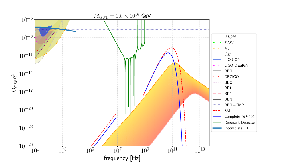
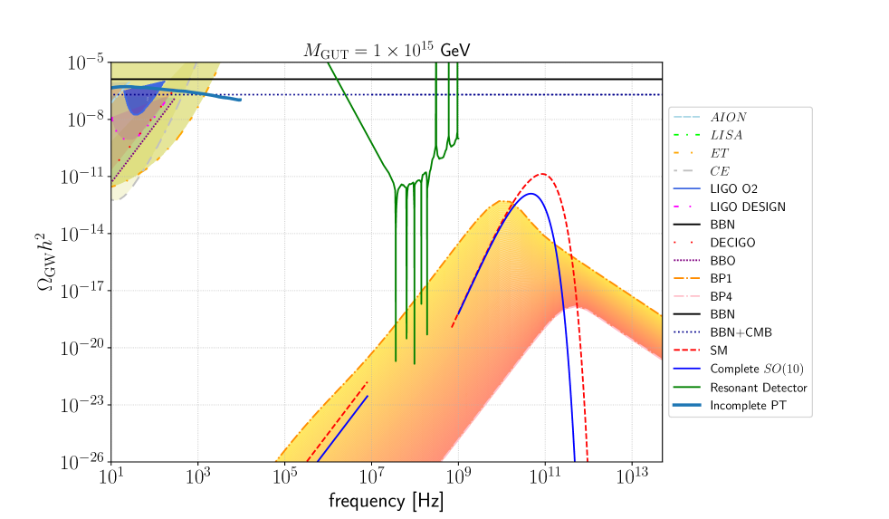
Figure 8: GW signals from the considered $SO(10)$ model for two different values of the unification scale, $M_{\text{GUT}}=1.6\times 10^{16}\,\text{GeV}$ (top) and $M_{\text{GUT}}=10^{15}\,\text{GeV}$ (bottom). The coloured region shows the GW spectrum that can be obtained from the FOPT at the GUT scale by varying the scalar quartic couplings within the allowed region of the parameter space; the upper boundary corresponds to BP 1, while the lower boundary is obtained for BP 4. Solid and dashed lines show the GW produced by fluctuations in the plasma, with the $SO(10)$ prediction plotted in blue, while the signal expected in the SM with the same reheating temperature is plotted in red for comparison. We also show the sensitivity of current and planned experiments, along with the BBN and the CMB constraints.

In Fig. 8 we plot all GW signals that we have considered in this work, along with some current and planned experiments, in particular the resonant detector proposed in [54]. As to the possibilities of observing GW produced by the scalar power spectrum when the phase transition is not completed before inflation (see Section 4), the details depend on the particular inflation scenario and are therefore more model-dependent. Nevertheless, in our scenario we can put a bound on the parameter $\gamma_{PT}$ that controls the shape and strength of the signal, $\gamma_{PT}\leq 10^{-3}\big{(}\Delta V(\phi)/\dot{\phi}_{\rm Inf}\big{)}^{2}$. We include this limit in Fig. 8. All possible signals that can come from this scenario will be lower than the solid petrol blue line shown from $10^{1}$ to $10^{4}$ Hz. We have not discussed GW produced by topological defects, which have been extensively studied recently (see, e.g., [9, 8, 55, 56, 57, 58, 59, 60, 61, 62]) and could occur at much lower frequencies.

We have studied a minimal GUT setup that realizes a realistic symmetry breaking chain. Although a direct solution to the Dark Matter problem is not given in this context, we have mentioned in Section 2.4 how the addition of a doublet of both $SU(2)_{L}$ and $SU(2)_{R}$ can provide a Dark Matter candidate, as some of us did in [30]. The fermion mass spectrum and perturbativity in the Higgs sector were not addressed but interestingly, both issues can be alleviated by introducing additional scalar fields at low energy. We have also made a number of simplifying assumptions about the mass spectrum and the contributions to the effective potential. Finally, the potential of a FOPT during the second step of symmetry breaking, which would produce GW with lower frequencies, warrants exploration. This study should therefore be considered a first step in the investigation of phase transitions in more complicated and more realistic unified models, paving the way for a promising new direction of research at the intersection of GUT model building and cosmology.

Appendix A SO(10) Group Theory

The generators of $SO(10)$ are conveniently labeled by antisymmetric indices, so we denote them by $T^{\alpha\beta}=-T^{\beta\alpha}$ with $\alpha,\beta=1,\dots,10$. In the fundamental representation, they are antisymmetric $10\times 10$ matrices,

$$(T^{\alpha\beta})_{ij}=-\frac{i}{\sqrt{2}}\left(\delta_{\alpha i}\delta_{\beta j}-\delta_{\alpha j}\delta_{\beta i}\right),$$ (A.1)

where $i,j=1,\dots,10$. We do not distinguish between upper and lower indices and imply summation over repeated indices. The generators satisfy

$$\operatorname{Tr}(T^{\alpha\beta}T^{\gamma\delta})=\delta_{\alpha\gamma}\delta_{\beta\delta}-\delta_{\alpha\delta}\delta_{\beta\gamma}\,.$$ (A.2)

The scalar and gauge boson fields relevant to our discussion transform under the adjoint representation $\mathbf{45}$ and are written as antisymmetric $10\times 10$ matrices as well,

$$\phi = \frac{i}{\sqrt{2}}\phi_{\alpha\beta}T^{\alpha\beta}\,,$$ (A.3)

$$A^{\mu} = \frac{i}{\sqrt{2}}A^{\mu}_{\alpha\beta}T^{\alpha\beta}\,.$$ (A.4)

Their Lagrangian is

$$\mathcal{L}=-\frac{1}{4}\operatorname{Tr}(F_{\mu\nu}F^{\mu\nu})+\frac{1}{4}\operatorname{Tr}\bigl{(}(D_{\mu}\phi)^{\dagger}(D^{\mu}\phi)\bigr{)}-V(\phi)\,,$$ (A.5)

where the scalar potential is given in Eq. (2.5). The field-strength tensor and the covariant derivative are given by

$$F^{\mu\nu} = \partial^{\nu}A^{\mu}-\partial^{\mu}A^{\nu}-ig\left[A^{\mu},A^{\nu}\right],$$ (A.6)

$$D^{\mu}\phi = \partial^{\mu}\phi-ig\left[A^{\mu},\phi\right].$$ (A.7)

In order to obtain the breaking pattern $SO(10)\to SU(3)_{c}\times SU(2)_{L}\times SU(2)_{R}\times U(1)_{B-L}$, we note that $SO(10)$ contains the subgroups $SO(6)$ and $SO(4)$, which are isomorphic to $SU(4)$ and $SU(2)_{L}\times SU(2)_{R}$, respectively. Defining the generators of $SU(4)$ as [63]

$$U_{1} =-\frac{1}{\sqrt{2}}\left(T^{36}+T^{45}\right), U_{8} =\frac{1}{\sqrt{6}}\left(2\,T^{12}-T^{34}+T^{56}\right),$$

$$U_{2} =-\frac{1}{\sqrt{2}}\left(T^{46}-T^{35}\right), U_{9} =-\frac{1}{\sqrt{2}}\left(T^{14}+T^{23}\right),$$

$$U_{3} =\frac{1}{\sqrt{2}}\left(T^{34}+T^{56}\right), U_{10} =\frac{1}{\sqrt{2}}\left(T^{13}-T^{24}\right),$$

$$U_{4} =\frac{1}{\sqrt{2}}\left(T^{16}+T^{25}\right), U_{11} =\frac{1}{\sqrt{2}}\left(T^{16}-T^{25}\right),$$

$$U_{5} =-\frac{1}{\sqrt{2}}\left(T^{15}-T^{26}\right), U_{12} =\frac{1}{\sqrt{2}}\left(T^{15}+T^{26}\right),$$

$$U_{6} =\frac{1}{\sqrt{2}}\left(T^{14}-T^{23}\right), U_{13} =\frac{1}{\sqrt{2}}\left(T^{36}-T^{45}\right),$$

$$U_{7} =\frac{1}{\sqrt{2}}\left(T^{13}+T^{24}\right), U_{14} =\frac{1}{\sqrt{2}}\left(T^{35}+T^{46}\right),$$

$$U_{15}=\frac{1}{\sqrt{3}}\left(T^{12}+T^{34}-T^{56}\right),$$ (A.8)

they satisfy

$$\operatorname{Tr}(U_{a}U_{b})=\delta_{ab}\quad,\quad a,b=1,\dots,15\,.$$ (A.9)

The generator $U_{15}$ commutes with both the $SO(4)$ generators and $U_{1,\dots,8}$, which generate the $SU(3)_{c}$ subgroup of $SU(4)$. Consequently, a vev $\braket{\phi}\propto U_{15}$ leads to the desired symmetry breaking with $U(1)_{B-L}$ generated by $U_{15}$.

Appendix B Effective Potential

Based on the previous discussion of symmetry breaking at the GUT scale, we consider a classical (or background) field proportional to the generator $U_{15}$,

$$\phi_{c}=\sqrt{2}i\,\varphi_{c}\,U_{15}\,,$$ (B.1)

where the factor $\sqrt{2}i$ ensures canonical normalization of the real scalar field $\varphi_{c}$. At the potential minimum,

$$\varphi_{c}=v\equiv\sqrt{3}\,\omega_{BL}\,.$$ (B.2)

Assuming that the symmetry breaking at the GUT scale is dominated by the single vev $v$, the effective potential can be approximated as a function of the single classical field $\varphi_{c}$.

The gauge boson masses after SSB are obtained by evaluating the commutators of the $SO(10)$ generators with $\braket{\phi}$ [15]. Likewise, we find the field-dependent mass matrix $M_{g}^{2}(\phi_{c})$, a $45\times 45$ matrix with elements

$$M_{g}^{2}(\phi_{c})_{(\alpha\beta)(\gamma\delta)}=\frac{g^{2}}{2}\operatorname{Tr}\left(\big{[}T^{(\alpha\beta)},\phi_{c}\big{]}\big{[}T^{(\gamma\delta)},\phi_{c}\big{]}\right),$$ (B.3)

where $(\alpha\beta)$ is an ordered index pair ($\alpha<\beta$) determining the row and analogously $(\gamma\delta)$ is an ordered pair determining the column. The block of $M_{g}^{2}$ containing the masses of the $24$ gauge bosons that do not belong to any of the subgroups in our breaking chain is diagonal with the non-zero entries $m_{g1}^{2}(\phi_{c})=\frac{1}{6}g^{2}\varphi_{c}^{2}$, see Tab. 1 where we collect the field-dependent masses of all particles relevant for our discussion. For the masses of the $SU(4)$ gauge bosons, the corresponding block of $M_{g}^{2}$ is not diagonal. Hence, it is more convenient to determine their masses in the basis of the $SU(4)$ generators, i.e., to calculate

$$M_{SU(4)}^{2}(\phi_{c})_{ab}=\frac{g^{2}}{2}\operatorname{Tr}\left(\big{[}U_{a},\phi_{c}\big{]}\big{[}U_{b},\phi_{c}\big{]}\right)$$ (B.4)

using the $SU(4)$ generators given in Eqs. (A.8). This yields $6$ massive gauge bosons with field-dependent masses squared $m_{g2}^{2}(\phi_{c})=\frac{2}{3}g^{2}\varphi_{c}^{2}$.

For the scalars, the field-dependent mass-squared matrix is given by

$$M^{2}_{s}(\phi_{c})_{(\alpha\beta)(\gamma\delta)}=\left.\frac{\partial^{2}\,V_{0}(\phi)}{\partial\phi_{(\alpha\beta)}\partial\phi_{(\gamma\delta)}}\right|_{\phi=\phi_{c}},$$ (B.5)

where $V_{0}(\phi)$ is the tree-level potential (2.5). Evaluating the eigenvalues of this matrix, we obtain the field-dependent scalar and NGB masses squared given in Tab. 1.

The thermal corrections are given by the well-known formulas [64, 47]

$$V_{\text{th}}(\phi_{c},T) = \sum_{i=g,s,\chi}\frac{n_{i}}{2\pi^{2}}T^{4}\,J_{b}(x)\quad,\quad x\equiv\frac{m_{i}(\phi_{c})}{T}\,,$$

$$J_{b}(x) = \Re\int_{0}^{\infty}dy\,y^{2}\ln\left[1-e^{-\sqrt{y^{2}+x^{2}}}\right],$$ (B.6)

where $n_{i}$ represents the degrees of freedom of particles. Also, note that we have to sum over the individual field-dependent gauge and scalar boson masses $m_{i}(\phi_{c})$ given in Tab. 1. As we do not consider Yukawa couplings between the fermions and the scalar $\mathbf{45}$, there is no fermionic contribution to the thermal corrections.

In Figs. 9 and 10 we present plots of the effective potential for the case of $M_{\text{GUT}}=1.6\times 10^{16}\,\text{GeV}$.

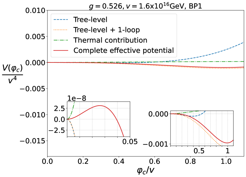
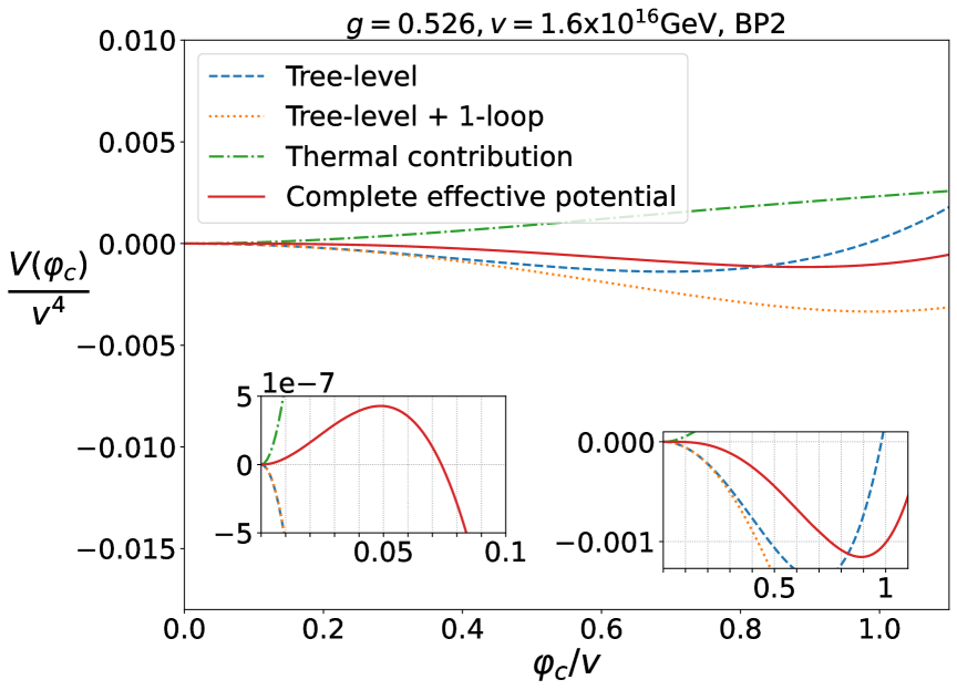
Figure 9: Effective potential for BP1 and BP2 for the case $M_{\text{GUT}}=1.6\times 10^{16}\,\text{GeV}$. The continuous red curve represents the complete $1$-loop effective potential $V(\phi_{c},T_{n})$ at the nucleation temperature.

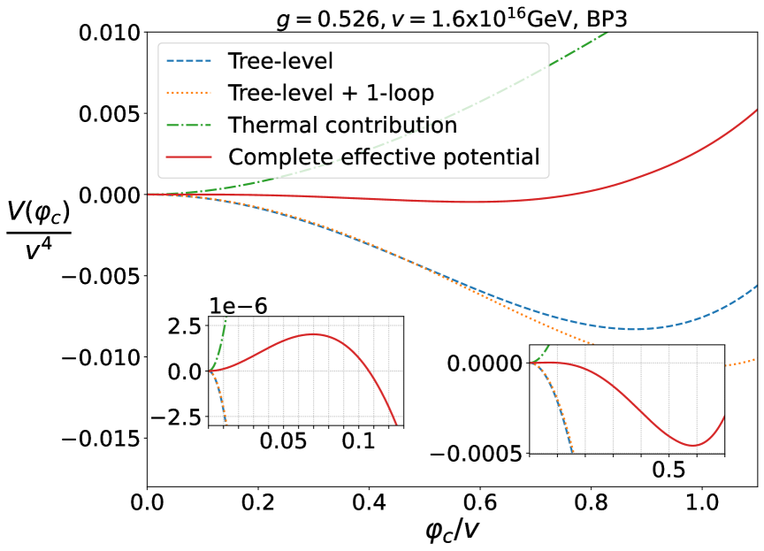
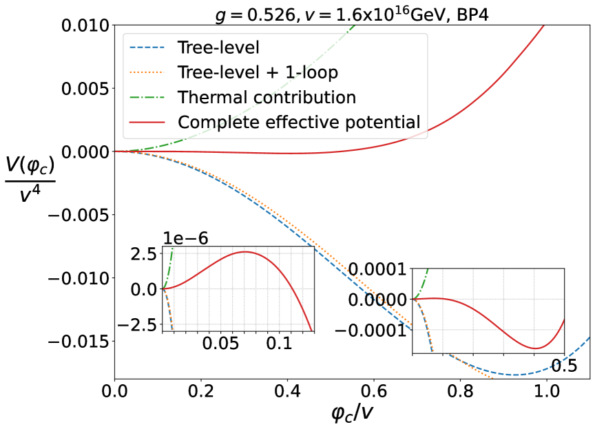
Figure 10: Same as Fig. 9 for BP3 and BP4.

Appendix C FOPT and GW Conventions

For completeness, we specify in this appendix the conventions we use for the FOPT parameters and the fits that we use for the density of GW. The 3D action describing the bubbles forming when the transition between the meta-stable and the true vacuum takes place is given by

$$S_{3}[\phi_{c}(r),T]=4\pi\int_{0}^{\infty}r^{2}dr\left[\frac{1}{2}\left(\frac{d\phi_{c}(r)}{dr}\right)^{2}+V(\phi_{c}(r),T)\right].$$ (C.1)

The strength of phase transition can be parameterized by

$$\alpha=\frac{1}{\rho_{\rm rad}}\left.\left[\Delta V(\phi_{c},T)-\frac{T}{4}\frac{\partial\Delta V(\phi_{c},T)}{\partial T}\right]\right|_{T=T_{n}},$$ (C.2)

where $\Delta V(\phi_{c},T)$ is the difference of the potential between the two minima (meta-stable and stable). The $\beta$ parameter quantifies the rate at which the FOPT occurs,

$$\beta=H_{*}\left.T\frac{d}{dT}\left(\frac{S_{3}}{T}\right)\right|_{T=T_{n}\approx T_{*}}.$$ (C.3)

The GW density is governed by the parameters $T_{n}$, $\alpha$, $\beta$, the sound speed, $c_{s}$, the bubble wall speed $v_{w}$, as well as the efficiency factors $\kappa_{\nu}$, and $\epsilon$. We employ these parameters in the well-known formulas [36, 37] for sound wave and turbulence contributions [43, 44] in the case where the barrier is mainly of thermal origin (i.e., it vanishes in the limit $T\rightarrow 0$) and the 1-loop gauge boson contributions are non-negligible. This is known as the case of non-runaway bubbles. In this case, the dominant contributions are sound waves and the magnetohydrodynamic (MHD) turbulence of the plasma.

The red-shifted sound wave contribution to the GW density observed today is

$$\Omega_{\rm sw}h^{2}(f)=\\ 2.65\times 10^{-6}\,H_{*}\tau_{\rm sw}\left(\frac{\beta}{H_{*}}\right)^{-1}v_{w}\left(\frac{\kappa_{\nu}\alpha}{1+\alpha}\right)^{2}\left(\frac{g_{*}}{100}\right)^{-\frac{1}{3}}\left(\frac{f}{f_{\rm sw}}\right)^{3}\left(\frac{7}{4+3\left(f/f_{\rm sw}\right)^{2}}\right)^{7/2},$$ (C.4)

where

$$f_{\rm{sw}}=1.9\times 10^{-5}\,\frac{1}{v_{w}}\left(\frac{\beta}{H_{*}}\right)\left(\frac{T_{*}}{100\,{\rm{GeV}}}\right)\left(\frac{g_{*}}{100}\right)^{1/6}{\rm{Hz}}$$ (C.5)

is the peak frequency as observed today. The factor $\tau_{\rm sw}=\min\left[\frac{1}{H_{*}},\frac{R_{*}}{\bar{U}_{f}}\right]$ is the time scale of the duration of the phase transition [45, 65], and $g_{*}$ and $H_{*}$, respectively, are the number of degrees of freedom in the thermal bath and the Hubble parameter at the time of GW production. For non-runaway bubbles, the reheating temperature and the thermal bath temperature, $T_{*}$, coincide with the nucleation temperature $T_{n}$. Thus, $\tau_{\rm sw}$ can equal either $1/H_{*}$ or ${R_{*}}/{\bar{U}_{f}}$, where $H_{*}R_{*}=\max(v_{w},c_{s})\,(8\pi)^{1/3}(\beta/H_{*})^{-1}$. The root-mean-square (RMS) fluid velocity can be approximated as

$$\bar{U}_{f}^{2}\approx\frac{3}{4}\left(\frac{\kappa_{\nu}\alpha}{1+\alpha}\right).$$

We emphasize that Eq. (C.4) is based on simulations that were restricted to values of $\alpha\lesssim 0.1$ and $\bar{U}_{f}\lesssim 0.05$ [66, 67]. The efficiency factor $\kappa_{\nu}$ can be approximated by [68]

$$\kappa_{\nu}\simeq\left\{\begin{array}[]{cc}\alpha(0.73+0.83\sqrt{\alpha}+\alpha)^{-1},&v_{w}\sim 1\,,\\ v_{w}^{6/5}6.9\alpha\left(1.36-0.037\sqrt{\alpha}+\alpha\right)^{-1},&v_{w}\ll 1\,.\end{array}\right.$$ (C.8)

The MHD turbulence provides a smaller contribution to the GW signal,

$$\Omega_{\text{turb}}h^{2}(f)=\\ 3.35\times 10^{-4}\left(\frac{\beta}{H_{*}}\right)^{-1}v_{w}\left(\frac{\epsilon\,\kappa_{\nu}\alpha}{1+\alpha}\right)^{\frac{3}{2}}\left(\frac{g_{*}}{100}\right)^{-\frac{1}{3}}\frac{\left(f/f_{\rm turb}\right)^{3}\left(1+f/f_{\rm turb}\right)^{-\frac{11}{3}}}{1+8\pi\frac{f}{h_{*}}}$$ (C.9)

with

$$h_{*}=16.5\frac{T_{*}}{10^{8}\,\rm{GeV}}\left(\frac{g_{*}}{100}\right)^{1/6}\text{Hz}$$ (C.10)

and the peak frequency

$$f_{\rm{turb}}=2.7\times 10^{-5}\,\frac{1}{v_{w}}\left(\frac{\beta}{H_{*}}\right)\left(\frac{T_{*}}{100\,{\rm{GeV}}}\right)\left(\frac{g_{*}}{100}\right)^{1/6}{\rm{Hz}}\,.$$ (C.11)

In Eq. (C.9) we have assumed that the turbulence efficiency factor $\kappa_{\rm t}$ can be written as $\kappa_{\rm{t}}=\epsilon\kappa_{\nu}$, where $\epsilon$ is another efficiency factor. As simulations suggest that at most $5\%$ to $10\%$ of the bulk motion of the bubble wall is converted into vorticity [37] (which enters into the turbulence contribution), it is customary to assume a conservative value of $\epsilon=0.05$ [66].

The bubble wall velocity $v_{w}$ is determined by a microphysical description of the interactions between the scalar field evolving through the bubble wall and the thermal plasma. As a precise computation is very challenging, we present the GW density profiles for the detonation velocity $v_{w}^{d}=(1/\sqrt{3}+\sqrt{\alpha^{2}+2\alpha/3})/(1+\alpha)$ [69]. The values $\epsilon=0.05$ and $\overline{U}_{f}\sim 0.05$ were obtained in the regime of detonations and small $\alpha$-deflagrations [37, 70, 66, 67].

References

- [1] M. Kamionkowski, A. Kosowsky and M.S. Turner, Gravitational radiation from first order phase transitions, Phys. Rev. D 49 (1994) 2837 [astro-ph/9310044].
- [2] NANOGrav collaboration, The NANOGrav 15 yr Data Set: Evidence for a Gravitational-wave Background, Astrophys. J. Lett. 951 (2023) L8 [2306.16213].
- [3] EPTA, InPTA collaboration, The second data release from the European Pulsar Timing Array – III. Search for gravitational wave signals, Astron. Astrophys. 678 (2023) A50 [2306.16214].
- [4] D.J. Reardon et al., Search for an Isotropic Gravitational-wave Background with the Parkes Pulsar Timing Array, Astrophys. J. Lett. 951 (2023) L6 [2306.16215].
- [5] H. Xu et al., Searching for the Nano-Hertz Stochastic Gravitational Wave Background with the Chinese Pulsar Timing Array Data Release I, Res. Astron. Astrophys. 23 (2023) 075024 [2306.16216].
- [6] R. Caldwell et al., Detection of early-universe gravitational-wave signatures and fundamental physics, Gen. Rel. Grav. 54 (2022) 156 [2203.07972].
- [7] NANOGrav collaboration, The NANOGrav 12.5 yr Data Set: Search for an Isotropic Stochastic Gravitational-wave Background, Astrophys. J. Lett. 905 (2020) L34 [2009.04496].
- [8] E.J. Chun and L. Velasco-Sevilla, Tracking down the route to the SM with inflation and gravitational waves, Phys. Rev. D 106 (2022) 035008 [2112.14483].
- [9] D.I. Dunsky, A. Ghoshal, H. Murayama, Y. Sakakihara and G. White, GUTs, hybrid topological defects, and gravitational waves, Phys. Rev. D 106 (2022) 075030 [2111.08750].
- [10] F.P. Huang and X. Zhang, Probing the gauge symmetry breaking of the early universe in 3-3-1 models and beyond by gravitational waves, Phys. Lett. B 788 (2019) 288 [1701.04338].
- [11] D. Croon, T.E. Gonzalo and G. White, Gravitational Waves from a Pati-Salam Phase Transition, JHEP 02 (2019) 083 [1812.02747].
- [12] V. Brdar, L. Graf, A.J. Helmboldt and X.-J. Xu, Gravitational Waves as a Probe of Left-Right Symmetry Breaking, JCAP 12 (2019) 027 [1909.02018].
- [13] J. Barir, M. Geller, C. Sun and T. Volansky, Gravitational waves from incomplete inflationary phase transitions, Phys. Rev. D 108 (2023) 115016 [2203.00693].
- [14] R. Jeannerot, J. Rocher and M. Sakellariadou, How generic is cosmic string formation in SUSY GUTs, Phys. Rev. D 68 (2003) 103514 [hep-ph/0308134].
- [15] L. Gráf, M. Malinský, T. Mede and V. Susič, One-loop pseudo-Goldstone masses in the minimal Higgs model, Phys. Rev. D 95 (2017) 075007 [1611.01021].
- [16] K. Jarkovská, M. Malinský, T. Mede and V. Susič, Quantum nature of the minimal potentially realistic SO(10) Higgs model, Phys. Rev. D 105 (2022) 095003 [2109.06784].
- [17] K. Jarkovská, M. Malinský and V. Susič, Trouble with the minimal renormalizable SO(10) GUT, Phys. Rev. D 108 (2023) 055003 [2304.14227].
- [18] T. Vachaspati and A. Achucarro, Semilocal cosmic strings, Phys. Rev. D 44 (1991) 3067.
- [19] M. Hindmarsh, Existence and stability of semilocal strings, Phys. Rev. Lett. 68 (1992) 1263.
- [20] A. Achúcarro, A. Avgoustidis, A. López-Eiguren, C.J.A.P. Martins and J. Urrestilla, Cosmological evolution of semilocal string networks, Phil. Trans. Roy. Soc. Lond. A 377 (2019) 0004 [1912.12069].
- [21] V.A. Rubakov, Superheavy Magnetic Monopoles and Proton Decay, JETP Lett. 33 (1981) 644.
- [22] C.G. Callan, Jr., Monopole Catalysis of Baryon Decay, Nucl. Phys. B 212 (1983) 391.
- [23] Planck collaboration, Planck 2018 results. X. Constraints on inflation, Astron. Astrophys. 641 (2020) A10 [1807.06211].
- [24] E.W. Kolb and M.S. Turner, The Early Universe, Taylor and Francis (2019), 10.1201/9780429492860.
- [25] A.J. Buras, Weak Hamiltonian, CP violation and rare decays, in Les Houches Summer School in Theoretical Physics, Session 68: Probing the Standard Model of Particle Interactions, pp. 281–539, 1998 [hep-ph/9806471].
- [26] T. Plehn, Lectures on LHC Physics, Lect. Notes Phys. 844 (2012) 1 [0910.4182].
- [27] Y. Mambrini, N. Nagata, K.A. Olive, J. Quevillon and J. Zheng, Dark matter and gauge coupling unification in nonsupersymmetric SO(10) grand unified models, Phys. Rev. D 91 (2015) 095010 [1502.06929].
- [28] J. Chakrabortty, R. Maji and S.F. King, Unification, Proton Decay and Topological Defects in non-SUSY GUTs with Thresholds, Phys. Rev. D 99 (2019) 095008 [1901.05867].
- [29] M.E. Machacek and M.T. Vaughn, Two Loop Renormalization Group Equations in a General Quantum Field Theory. 3. Scalar Quartic Couplings, Nucl. Phys. B 249 (1985) 70.
- [30] A. Biswas, A. Kar, H. Kim, S. Scopel and L. Velasco-Sevilla, Improved white dwarves constraints on inelastic dark matter and left-right symmetric models, Phys. Rev. D 106 (2022) 083012 [2206.06667].
- [31] J. Ellis, J.L. Evans, N. Nagata, K.A. Olive and L. Velasco-Sevilla, Supersymmetric proton decay revisited, Eur. Phys. J. C 80 (2020) 332 [1912.04888].
- [32] Super-Kamiokande collaboration, Search for proton decay via and in 0.31 megaton·years exposure of the Super-Kamiokande water Cherenkov detector, Phys. Rev. D 95 (2017) 012004 [1610.03597].
- [33] Hyper-Kamiokande collaboration, Hyper-Kamiokande Design Report, 1805.04163.
- [34] M.B. Hindmarsh, M. Lüben, J. Lumma and M. Pauly, Phase transitions in the early universe, SciPost Phys. Lect. Notes 24 (2021) 1 [2008.09136].
- [35] S.J. Huber and T. Konstandin, Gravitational Wave Production by Collisions: More Bubbles, JCAP 09 (2008) 022 [0806.1828].
- [36] M. Hindmarsh, S.J. Huber, K. Rummukainen and D.J. Weir, Gravitational waves from the sound of a first order phase transition, Phys. Rev. Lett. 112 (2014) 041301 [1304.2433].
- [37] M. Hindmarsh, S.J. Huber, K. Rummukainen and D.J. Weir, Numerical simulations of acoustically generated gravitational waves at a first order phase transition, Phys. Rev. D 92 (2015) 123009 [1504.03291].
- [38] A. Kosowsky, A. Mack and T. Kahniashvili, Gravitational radiation from cosmological turbulence, Phys. Rev. D 66 (2002) 024030 [astro-ph/0111483].
- [39] A. Nicolis, Relic gravitational waves from colliding bubbles and cosmic turbulence, Class. Quant. Grav. 21 (2004) L27 [gr-qc/0303084].
- [40] C. Caprini and R. Durrer, Gravitational waves from stochastic relativistic sources: Primordial turbulence and magnetic fields, Phys. Rev. D 74 (2006) 063521 [astro-ph/0603476].
- [41] T. Kahniashvili, A. Brandenburg, L. Campanelli, B. Ratra and A.G. Tevzadze, Evolution of inflation-generated magnetic field through phase transitions, Phys. Rev. D 86 (2012) 103005 [1206.2428].
- [42] L. Kisslinger and T. Kahniashvili, Polarized Gravitational Waves from Cosmological Phase Transitions, Phys. Rev. D 92 (2015) 043006 [1505.03680].
- [43] C. Caprini, R. Durrer and G. Servant, The stochastic gravitational wave background from turbulence and magnetic fields generated by a first-order phase transition, JCAP 12 (2009) 024 [0909.0622].
- [44] P. Binetruy, A. Bohe, C. Caprini and J.-F. Dufaux, Cosmological Backgrounds of Gravitational Waves and eLISA/NGO: Phase Transitions, Cosmic Strings and Other Sources, JCAP 06 (2012) 027 [1201.0983].
- [45] J. Ellis, M. Lewicki and J.M. No, On the Maximal Strength of a First-Order Electroweak Phase Transition and its Gravitational Wave Signal, JCAP 04 (2019) 003 [1809.08242].
- [46] S. Coleman, Fate of the false vacuum: Semiclassical theory, Phys. Rev. D 15 (1977) 2929.
- [47] A.D. Linde, Decay of the False Vacuum at Finite Temperature, Nucl. Phys. B 216 (1983) 421.
- [48] A.D. Linde, Fate of the false vacuum at finite temperature: Theory and applications, Phys. Lett. B 100 (1981) 37.
- [49] J. Ghiglieri and M. Laine, Gravitational wave background from Standard Model physics: Qualitative features, JCAP 07 (2015) 022 [1504.02569].
- [50] J. Ghiglieri, G. Jackson, M. Laine and Y. Zhu, Gravitational wave background from Standard Model physics: Complete leading order, JHEP 07 (2020) 092 [2004.11392].
- [51] E. Braaten and R.D. Pisarski, Soft Amplitudes in Hot Gauge Theories: A General Analysis, Nucl. Phys. B 337 (1990) 569.
- [52] H.A. Weldon, Effective Fermion Masses of Order gT in High Temperature Gauge Theories with Exact Chiral Invariance, Phys. Rev. D 26 (1982) 2789.
- [53] R.M. Fonseca, GroupMath: A Mathematica package for group theory calculations, Comput. Phys. Commun. 267 (2021) 108085 [2011.01764].
- [54] N. Herman, L. Lehoucq and A. Fúzfa, Electromagnetic antennas for the resonant detection of the stochastic gravitational wave background, Phys. Rev. D 108 (2023) 124009 [2203.15668].
- [55] S. Antusch, K. Hinze, S. Saad and J. Steiner, Singling out SO(10) GUT models using recent PTA results, Phys. Rev. D 108 (2023) 095053 [2307.04595].
- [56] W. Buchmüller, V. Domcke and K. Schmitz, Metastable cosmic strings, JCAP 11 (2023) 020 [2307.04691].
- [57] G. Lazarides, R. Maji, A. Moursy and Q. Shafi, Inflation, superheavy metastable strings and gravitational waves in non-supersymmetric flipped SU(5), JCAP 03 (2024) 006 [2308.07094].
- [58] W. Ahmed, M.U. Rehman and U. Zubair, Probing stochastic gravitational wave background from strings in light of NANOGrav 15-year data, JCAP 01 (2024) 049 [2308.09125].
- [59] S.F. King, G.K. Leontaris and Y.-L. Zhou, Flipped SU(5): unification, proton decay, fermion masses and gravitational waves, JHEP 03 (2024) 006 [2311.11857].
- [60] S. Antusch, K. Hinze and S. Saad, Explaining PTA results by metastable cosmic strings from SO(10) GUT, JCAP 10 (2024) 007 [2406.17014].
- [61] R. Maji and Q. Shafi, C-parity, magnetic monopoles, and higher frequency gravitational waves, Phys. Rev. D 111 (2025) 075027 [2502.10135].
- [62] R. Maji and Q. Shafi, Superheavy Metastable Strings in SO(10), 2504.09055.
- [63] A.D. Özer, - Grand Unification and Fermion Masses, Ph.D. thesis, Munich U., 2005. 10.5282/edoc.4695.
- [64] L. Dolan and R. Jackiw, Symmetry behavior at finite temperature, Phys. Rev. D 9 (1974) 3320.
- [65] J. Ellis, M. Lewicki, J.M. No and V. Vaskonen, Gravitational wave energy budget in strongly supercooled phase transitions, JCAP 06 (2019) 024 [1903.09642].
- [66] C. Caprini et al., Science with the space-based interferometer eLISA. II: Gravitational waves from cosmological phase transitions, JCAP 04 (2016) 001 [1512.06239].
- [67] C. Caprini et al., Detecting gravitational waves from cosmological phase transitions with LISA: an update, JCAP 03 (2020) 024 [1910.13125].
- [68] J.R. Espinosa, T. Konstandin, J.M. No and G. Servant, Energy Budget of Cosmological First-order Phase Transitions, JCAP 06 (2010) 028 [1004.4187].
- [69] P.J. Steinhardt, Relativistic detonation waves and bubble growth in false vacuum decay, Phys. Rev. D 25 (1982) 2074.
- [70] M. Hindmarsh, S.J. Huber, K. Rummukainen and D.J. Weir, Shape of the acoustic gravitational wave power spectrum from a first order phase transition, Phys. Rev. D 96 (2017) 103520 [1704.05871].