When Measurement Mediates the Effect of Interest

Abstract

Many health promotion strategies aim to improve reach into the target population and outcomes among those reached. For example, an HIV prevention strategy could expand the reach of risk screening and the delivery of biomedical prevention to persons with HIV risk. This setting creates a complex missing data problem: the strategy improves health outcomes directly and indirectly through expanded reach, while outcomes are only measured among those reached. To formally define the total causal effect in such settings, we use Counterfactual Strata Effects: causal estimands where the outcome is only relevant for a group whose membership is subject to missingness and/or impacted by the exposure. To identify and estimate the corresponding statistical estimand, we propose a novel extension of Two-Stage targeted minimum loss-based estimation (TMLE). Simulations demonstrate the practical performance of our approach as well as the limitations of existing approaches.

Key Words: cluster-randomized control trials; missing data; mediation; targeted minimum loss-based estimation; counterfactual strata effects:

1 Introduction

Missing data remain a persistent challenge in medical and public health research [1]. Persons with complete data on key variables often differ meaningfully from persons with missing data. Failure to account for these differences can lead to biased estimates and precision losses [2, 3, 4]. Common approaches to handle missing data include (1) a ”complete-case analysis”, which restricts to participants with the relevant variables measured, (2) adjustment for baseline factors (e.g., age and sex) through standardization (i.e., G-computation) or inverse weighting, and (3) multiple imputation [5, 6, 7]. These approaches are not directly applicable when the total effect is of interest and measurement mediates the causal effect.

Concretely, health screening is often the first step to initiating a new treatment or prevention product. For example, HIV testing is a prerequisite for initiation of antiretroviral therapy (ART) for persons with HIV and for initiation of pre-exposure prophylaxis (PrEP) for persons at risk of HIV acquisition. Similarly, blood pressure must be measured prior to starting antihypertensive medication, and LDL cholesterol must be measured prior to starting Statins. However, the coverage of health screening is never 100%, and the target population of our prevention/treatment efforts is generally unknown (e.g., [8, 9]). Therefore, implementation strategies to improve health outcomes often also aim to improve the reach of health screening. For example, a strategy could expand outreach and service delivery into the community through village health teams or peer-based approaches (e.g., [10, 11, 12]). Likewise, a strategy could improve screening and uptake by integrating services at the health clinic or by offering new services at a pharmacy (e.g., [13, 14]).

In such settings, the strategy is often deployed at the group-level or induces changes at the group-level. Examples of groups include communities, pharmacies, clinics, and health systems. Also in such settings, health screening is a mediator; it is an intermediate variable on the causal pathway between the exposure (a health promotion strategy) and the outcome (treatment/prevention uptake) [15, 16, 17, 18, 19, 20]. Several mediated effects may be of potential interest, including controlled direct effects, natural direct and indirect effects, stochastic direct and indirect effects, and separable direct and indirect effects [17, 21, 22, 23, 24]. These estimands correspond to hypothetical interventions to change the distribution of the mediator and are reviewed in Rudolph et al. [25]. However, when studying a novel health promotion strategy, it is of primary interest to evaluate the total causal effect, prior to investigating mediating pathways.

We present a general framework to evaluate total effects of strategies that simultaneously improve reach into the target population and outcomes among those reached. Specifically, we provide a framework to address the novel multilevel-mediation-missing data problem, arising because (1) the group-level intervention improves health outcomes directly and indirectly through expanded reach; (2) simultaneously, outcomes are only measured among those reached. First, we give an overview of the motivating study, a cluster randomized trial (CRT) to improve PrEP uptake in rural Kenya and Uganda. Next, we describe the data generation process with a hierarchical causal model and formally define the causal estimand with Counterfactual Strata Effects, occurring when the outcome is only relevant for a group whose membership is subject to missingness and/or impacted by the exposure [26, 27, 28, 29, 30]. For identification and estimation of the corresponding statistical estimand, we use Two-Stage targeted minimum loss-based estimation (TMLE), which separates control for missing data from effect evaluation [27]. Our simulation study evaluates the finite sample performance of our approach and compares with alternatives. We close with a discussion of extensions to more complex settings and areas for ongoing research. To match our motivating example, we focus on CRTs throughout.

2 Motivating Study

Alcohol use is a persistent risk factor for HIV acquisition [31, 32, 33, 34, 35, 36, 37, 38] . In sub-Saharan Africa, attending drinking venues (i.e., bars) as a patron or an employee has been associated with increased HIV risk [39, 40, 41]. OPAL (Outreach and Prevention at ALcohol venues) is an ongoing CRT whose primary objective is to evaluate the effectiveness of community-based, recruitment strategies on PrEP uptake among adults at drinking venues in rural Kenya and Uganda (NCT05862857). The units of randomization (i.e., clusters) are groups of nearby drinking venues. At these venues, patrons and employees receive recruitment cards offering multi-disease screening (intervention) or HIV-focused screening (control) at their local health clinic. When these cards are presented at the clinic, the participant is offered screening as well as PrEP initiation if interested and eligible. The primary research question is what would be the difference in PrEP uptake among persons with HIV risk if everyone received a multi-disease versus HIV-focused recruitment card.

Figure 1 provides a simplified schematic of OPAL and illustrates the multilevel-mediation-missing data problem inherent in studies aiming to expand reach into the target population and health outcomes among those reached. First, CRTs have a hierarchical data structure; individuals are nested in clusters. Second, risk screening mediates the effect on prevention use. There is a direct effect of the intervention on prevention use as well as an indirect effect through risk screening. Third, everyone has an “underlying” HIV risk status, which is only observed if they participate in screening. In other words, HIV risk status is missing unless they engage in screening, which is also a prerequisite for starting PrEP. Existing methods for missing data would adjust for differences between persons screened versus not screened. However, these methods would block the indirect effect and bias estimates of overall effectiveness towards the null. We now present our novel approach for estimating total effects, while addressing the multilevel-mediation-missing data problem, common to CRTs aiming to improve reach into the target population and health outcomes among persons reached.

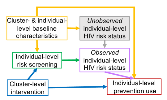
Figure 1: Simplified causal graph for the OPAL trial to increase HIV risk screening and prevention use among persons with HIV risk: individuals are nested within clusters; HIV risk screening mediates the intervention effect, and HIV risk status is missing (unobserved) if an individual does not screen. New methods are needed to evaluate overall effectiveness, while accounting for the multilevel-mediation-missing data problem.

3 Methods

We first introduce the notation that will be used to formalize the data generating process, specify the causal estimand, and derive the statistical estimand. Throughout, clusters are indexed with $j=\{1,\ldots,J\}$, and individuals are indexed with $i=\{1,\ldots,N_{j}\}$. The number of individuals in a given cluster $N_{j}$ often varies. Cluster-level variables are indexed by super-script $c$ and shared by all individuals in that cluster. For the $j^{th}$ cluster, $E^{c}_{j}$ denotes the cluster-level baseline covariates, and $A^{c}_{j}=1$ denotes randomization to the intervention arm, while $A^{c}_{j}=0$ denotes randomization to the control arm. Bold font denotes the set of individual-level variables for a given cluster. For the $N_{j}$ individuals in the $j^{th}$ cluster, $\bm{W}_{j}$ is the matrix of individual-level characteristics at baseline:

$$\bm{W}_{j}=\begin{bmatrix}W1_{1j}&W2_{1j}&\cdots\\ W1_{2j}&W2_{2j}&\cdots\\ \vdots&\vdots&\vdots\\ W1_{N_{j}j}&W2_{N_{j}j}&\cdots\end{bmatrix}$$

In OPAL, for example, $\bm{W}_{j}$ could include the age, sex, alcohol use, mobility, and socioeconomic status for the individuals in cluster $j$.

Asterisks denote underlying values of variables. In OPAL, $\bm{Y1}_{j}^{*}=(Y1_{ij}^{*}:i=1,...,N_{j})$ is the vector of underlying indicators of HIV risk for the $N_{j}$ individuals from cluster $j$. More generally, $Y1$ is an indicator of being in the target population of interest (e.g., having HIV for the outcome of ART initiation or having high blood pressure for the outcome of antihypertensive medication use). These indicators are only observed for individuals participating in health screening. Therefore, we define $\bm{\Delta}_{j}=(\Delta_{ij}:i=1,\ldots,N_{j}$) as the vector of measurement indicators for cluster $j$. In OPAL, the HIV risk status of given individual is observed if they are screened at the health center (i.e., if $\Delta$=1) and is missing otherwise (i.e., if $\Delta$=0). Then we define the observed indicators as $Y1_{ij}=\Delta_{ij}\times Y1_{ij}^{*}$ for individual $i$ in cluster $j$ and as $\bm{Y1}_{j}=(Y1_{ij}:i=1,\ldots,N_{j}$) for cluster $j$. In OPAL, $Y1=1$ if the individual screened at risk for HIV acquisition and is zero otherwise (i.e., screened but was not at risk, or did not screen). Finally, we define the outcome vector for cluster $j$ as $\bm{Y2}_{j}=(Y2_{ij}:i=1,\ldots,N_{j}$). In OPAL, $\bm{Y2}$ consists of indicators of PrEP initiation. To match the running example where PrEP initiation occurs at the health clinic, we assume complete measurement, but this can easily be relaxed. Altogether, we denote the observed data for individual $i$ in cluster $j$ as $O_{ij}=(E^{c}_{j},W_{ij},A^{c}_{j},\Delta_{ij},Y1_{ij},Y2_{ij})$.

3.1 Structural causal model

Causal relationships between these variables are specified through a hierarchical, non-parametric structural equation model [42, 43]:

$$E^{c} =f_{E^{c}}(U_{E^{c}})$$

$$\bm{W} =f_{\bm{W}}(E^{c},U_{\bm{W}})$$

$$A^{c} =f_{A^{c}}(U_{A^{c}})$$

$$\bm{Y1}^{*} =f_{\bm{Y1}^{*}}(E^{c},\bm{W},U_{\bm{Y1}^{*}})$$

$$\bm{\Delta} =f_{\bm{\Delta}}(E^{c},\bm{W},A^{c},U_{\bm{\Delta}})$$

$$\bm{Y1} =\bm{\Delta}\times\bm{Y1}^{*}$$

$$\bm{Y2} =f_{\bm{Y2}}(E^{c},\bm{W},A^{c},\bm{Y1},U_{\bm{Y2}})$$

In this model, the values of the random variables on the left-hand side are determined by the structural equations $(f_{E^{c}},f_{\bm{W}},f_{A^{c}},f_{\bm{Y1}^{*}},f_{\bm{\Delta}},f_{\bm{Y1}},f_{\bm{Y2}})$, which are non-parametric, and specify each variable’s “parents”, including unmeasured factors $(U_{E^{c}},U_{\bm{W}},U_{A^{c}},U_{\bm{Y1}^{*}},U_{\bm{\Delta}},U_{\bm{Y2}})$. Due to randomization, the unmeasured factors contributing to the intervention assignment $U_{A^{c}}$ are independent of the others. The corresponding directed acyclic graph is given in Figure 2.

To reflect the OPAL study, we have made several exclusion restrictions. First, the trial arm $A^{c}$ is completely randomized; this assumption can easily be relaxed to reflect covariate-dependent randomization schemes. Second, there is no impact of the trial arm $A^{c}$ on underlying HIV risk status $\bm{Y1}^{*}$. In other words, we assume the intervention does not impact the target population of interest. We relax this and other assumptions in Section 5. Third, there is no effect of underlying risk status $\bm{Y1}^{*}$ on screening $\bm{\Delta}$; this assumption is needed for identification, as detailed below (Section 3.4). Finally, by definition, observed HIV risk status $\bm{Y1}$ is only a function of underlying risk status $\bm{Y1}^{*}$ and measurement $\bm{\Delta}$. Using the causal model, we can generate counterfactuals and formally define the causal estimand of interest, as described next.

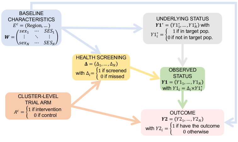
Figure 2: A simplified hierarchical causal graph to illustrate the data generating process in a CRT where the intervention improves health screening and health outcomes (among those screened). Since the causal model is defined at the cluster-level, we drop the subscript $j$ throughout. For simplicity, we have omitted the unmeasured factors: $\bm{U}=(U_{E^{c}},U_{\bm{W}},U_{A^{c}},U_{\bm{Y1}^{*}},U_{\bm{\Delta}},U_{\bm{Y2}})$.

3.2 Counterfactual Strata Effects

Recall our goal is to estimate the total effect: a contrast in the expected counterfactual outcome under the intervention versus the expected counterfactual outcome under the control. In OPAL, for example, our goal is to evaluate the expected difference in the counterfactual probability of starting PrEP for persons with HIV risk if all clusters received multi-disease recruitment cards ($A^{c}=1$) versus HIV-only recruitment cards ($A^{c}=0$). Our causal effect of interest is formally defined as

$$\Psi^{*}=\mathbb{E}[Y^{c*}(1)-Y^{c*}(0)]$$

where the expectation is over the target population of clusters and where

$$Y^{c*}(a^{c})=\mathbb{P}[Y2(a^{c})=1\mid Y1^{*}=1]$$

is the counterfactual probability of starting PrEP under trial arm $a^{c}$, among persons at risk of HIV acquisition. Of course, we could consider alternative contrasts (e.g., ratios) and alternative summaries (e.g., weighting by cluster size) [44]. Crucially, our causal parameter $\Psi^{*}$ is a summary of counterfactual outcomes under the two strategies of interest, but does not modify measurement. In other words, $\Psi^{*}$ captures the direct and indirect effects of the intervention in the target population without enforcing 100% compliance on screening. Therefore, $\Psi^{*}$ is an intent-to-treat parameter.

Due to the conditioning on underlying variables, causal parameters of this type have been termed “Counterfactual Strata Effects” [30, 29]. Counterfactual Strata Effects are causal estimands where the outcome is only relevant for a group whose membership is subject to missingness and/or impacted by the exposure. In the running example, PrEP uptake is only relevant for persons who are at risk of HIV acquisition, and the population with HIV risk is generally unknown. Counterfactual Strata Effects have previously been applied to study intervention effects on population-level HIV viral suppression (the proportion of all persons with HIV who are suppressing viral replication) and the incidence of latent tuberculosis infection (the proportion of persons at risk of tuberculosis who acquire it) [45, 27, 46, 47, 26, 28, 48, 49]. In both examples, the outcome and the target population are subject to missingness, and the study intervention may have had an impact on the target population. (See extensions in Section 5.)

Counterfactual Strata Effects are related but distinct from Principal Strata Effects [50, 51]. In the latter, effects are defined conditional on latent classes where a post-baseline variable is used to cross-classify participants by joint potential values of that variable under each exposure level. Examples include average causal effects among compliers, defiers, always takers, or never takers. In OPAL, for example, we could estimate the average treatment effect among the latent subgroup of persons who would be always be screened for PrEP eligibility regardless of the recruitment card that they received. However, our goal is to evaluate the overall effectiveness of the health strategy among the entire target population.

Counterfactual Strata Effects are also related but distinct from the framework proposed by Young and colleagues for time-to-event outcomes with competing events [23, 24, 52, 53]. Specifically, when the competing event is a censoring event, contrasts of the expected counterfactual outcomes define a controlled direct effect: the impact if all censoring had been prevented. To understand how the competing event mediates the causal effect in such settings, Young and colleagues have also proposed separable direct and indirect effects. However, our goal remains to evaluate the total effect of the health promotion strategy among persons in the target population, including those not reached for health screening. We now propose developing, evaluating, and applying Two-Stage TMLE for this effect.

3.3 Two-Stage TMLE for Estimation and Inference

Two-Stage TMLE is a general approach to identifying and estimating causal effects in a settings with missing data and dependent data [27, 28]. In the first stage, we fully stratify on each cluster and focus on controlling for differential missingness/censoring of individual-level data. In the second stage, we use estimates from the first stage to evaluate the total effect and focus on improving efficiency. In the following, we propose an implementation of Two-Stage TMLE to address unique challenges when evaluating the total effect of strategies to improve reach into the target population and outcomes among those reached. As detailed below, fully stratifying on each cluster in the first stage simplifies the multilevel-mediation-missingness problem (Figure 1). Therefore, we can control for differential measurement without losing the effect of the cluster-level exposure (i.e., without blocking the indirect effect).

3.4 Stage 1: Identifying and estimating in each cluster

In Stage 1, we consider each cluster in turn. Within each cluster, the cluster-level covariates and intervention are constant. Therefore, the observed data for cluster $j$ simplify to $O_{ij}=(W_{ij},\Delta_{ij},Y1_{ij},Y2_{ij})$ for $i=1,\ldots,N_{j}$. Equally importantly, our Stage 1 causal estimand simplifies to the counterfactual probability of the outcome for persons in the target population: $Y^{c*}$= $\mathbb{P}(Y2=1\mid Y1^{*}=1)$. In OPAL, this is the probability of initiating PrEP among persons with HIV risk. Crucially, stratifying on cluster allows the missingness mechanism to vary by cluster, while capturing the impacts of the cluster-level variables, including the intervention $A^{c}$.

Following [45, 26, 27, 28], we re-express this causal estimand as the joint probability of being in the target population and having the outcome, divided by the probability of being in the target population:

$$Y^{c*}=\frac{\mathbb{P}(Y2=1,Y1^{*}=1)}{\mathbb{P}(Y1^{*}=1)}$$

In OPAL, $Y^{c*}$ is now written as the joint probability of initiating PrEP and being at risk of HIV acquisition, divided by the prevalence of HIV risk. The numerator and denominator can then be identified and estimated, separately.

We first focus on the numerator. Throughout, having the outcome is contingent on being in the target population (e.g., starting PrEP is contingent upon on testing HIV-negative and reporting risk). Therefore, the numerator simplifies to the observed proportion with the outcome: $\mathbb{P}(Y2=1)$. This framework naturally extends to more complex settings where the outcome is also subject to missingness [26, 27, 28].

We now turn to the denominator. Throughout, the denominator defines the target population and is subject to missingness: $\mathbb{P}(Y1^{*}=1)$. To identify the denominator from the observed data distribution, we need to consider the plausibility of various missing data assumptions. Suppose the missing-completely-at-random (MCAR) held within each cluster [3]. For a given cluster in OPAL, the corresponding assumption would be that HIV risk among persons who go to the clinic for screening is perfectly representative of HIV risk among persons who do not. This is highly implausible, and we, instead, consider the missing-at-random (MAR) assumption [3]: for each cluster, HIV risk among those screened is representative of risk among those missed within all possible values of the baseline covariates $W$. Importantly, the adjustment set for a given individual can include covariates of other cluster members (e.g., their friends). Furthermore, in OPAL where a cluster is a group of nearby drinking venues, the adjustment set can also include characteristics of the venue (e.g., type of alcohol served or presence of on-site rooms for sex work). This missing data assumption can be represented as $Y1^{*}\perp\Delta\mid W$ and is further relaxed in Section 5 to adjust for time-varying covariates, which are potentially impacted by the exposure $A^{c}$. Additionally, we require that the probability of being measured within covariate strata be bounded away from 0: $\mathbb{P}(\Delta=1\mid W=w)>0$ for all possible $w$. Under these assumptions, the statistical estimand for the denominator is given by the G-computation formula [54]: $\mathbb{E}[\mathbb{E}(Y1\mid\Delta=1,W)]$.

Altogether, our Stage 1 statistical estimand, a cluster-level parameter, is

$$Y^{c}=\frac{\mathbb{P}(Y2=1)}{\mathbb{E}[\mathbb{E}(Y1\mid\Delta=1,W)]}$$

In OPAL, $Y^{c}$ is interpreted as the probability of starting PrEP, divided the adjusted prevalence of HIV risk. To estimate the numerator, we use the empirical proportion with the outcome. To estimate the denominator, we use TMLE, a doubly robust, substitution estimator optimizing the bias-variance trade-off for the target parameter [55]. Within TMLE, we apply the Super Learner, an ensemble machine learning algorithm [56], for flexible estimation of the the outcome regression $\mathbb{E}(Y1\mid\Delta=1,W)$ and measurement mechanism $\mathbb{P}(\Delta=1\mid W)$. Briefly, the TMLE algorithm updates the initial estimates of $\hat{\mathbb{E}}(Y1\mid\Delta=1,W)$ by using information from $\hat{\mathbb{P}}(\Delta=1\mid W)$ and obtains targeted estimates $\hat{\mathbb{E}}^{\star}(Y1\mid\Delta=1,W)$, which are averaged across individuals.

Since we fully stratify on cluster in Stage 1, we need to implement the estimation algorithm $J$ times to obtain estimates for each cluster $j=\{1,\ldots,J\}$:

$$\hat{Y}_{j}^{c}=\frac{1/N_{j}\sum_{i=1}^{N_{j}}\mathbbm{1}(Y2_{ij}=1)}{1/N_{j}\sum_{i=1}^{N_{j}}\hat{\mathbb{E}}^{\star}(Y1\mid\Delta=1,W_{ij})}$$

To obtain confidence intervals for these estimates $\hat{Y}^{c}$, we apply the Delta method to the influence curve of the numerator and denominator.

3.5 Stage 2: Identifying and estimating the total effect

Stage 1 focuses on identifying and estimating the expected outcome among the underlying target population for each cluster. However, recall our primary research question is the total effect of the health promotion strategy: $\Psi^{*}=\mathbb{E}[Y^{c*}(1)-Y^{c*}(0)]$. In OPAL, $\Psi^{*}$ is the expected difference in the counterfactual uptake of PrEP (among persons with HIV risk) if all clusters received multi-disease messaging $Y^{c}$(1) versus HIV-focused messaging $Y^{c}$(0). In Stage 2, we focus on evaluating the total effect $\Psi^{*}$ with maximum precision. In Stage 2, the observed data are at the cluster-level and given by $O^{c}=(E^{c},W^{c},A^{c},\hat{Y}^{c})$, where $W^{c}$ denote aggregates of the individual-level baseline covariates W and $\hat{Y}^{c}$ are the cluster-level endpoint estimates from Stage 1.

Due to randomization of the trial arms and complete follow-up of clusters, we can obtain a point estimate of the total effect by simply contrasting the arm-specific average outcomes (i.e., implementing an unadjusted effect estimator):

$$\hat{\Psi}_{unadj}=\frac{1}{J}\sum_{j=1}^{J}\mathbbm{1}(A^{c}=1)(\hat{Y}^{c}_{j})-\mathbbm{1}(A^{c}=0)(\hat{Y}^{c}_{j})$$ (1)

However, statistical precision and power can be improved by adjusting for baseline covariates that are predictive of the outcome [57, 58, 59, 60, 61, 44, 27]. Therefore, we implement a cluster-level TMLE to obtain a more efficient estimate of the total effect. Briefly, an initial estimate of the cluster-level outcome regression $\hat{\mathbb{E}}(\hat{Y}^{c}\mid A^{c}=a^{c},E^{c},W^{c})$ is updated using information in the cluster-level propensity score $\hat{\mathbb{P}}(A^{c}=1\mid E^{c},W^{c})$. Then targeted estimates of the expected outcome under each trial arm are averaged to obtain a point estimate:

$$\hat{\Psi}_{tmle}=\frac{1}{J}\sum_{j=1}^{J}\hat{\mathbb{E}}^{\star}(\hat{Y}^{c}\mid A^{c}=1,E^{c}_{j},W^{c}_{j})-\hat{\mathbb{E}}^{\star}(\hat{Y}^{c}\mid A^{c}=0,E^{c}_{j},W^{c}_{j})$$ (2)

In a trial setting, we implement TMLE with Adaptive Pre-specification to data-adaptively select the adjustment approach that maximizes empirical efficiency [62, 63]. In this procedure, we pre-specify candidate algorithms for estimation of the outcome regression and the known propensity score. In trials with few clusters, we recommend limiting these algorithms to “working” generalized linear models (GLMs) adjusting for a single covariate. In trials with many clusters, we can expand the candidate set to include more adaptive approaches adjusting for multiple covariates (e.g., stepwise regression and multivariate adaptive regression splines). In addition, we pre-specify the loss function to be the squared of the influence curve of the cluster-level TMLE; the expectation of this loss function is the variance of the TMLE. Finally, we pre-specify a cross-validation scheme to evaluate performance and collaboratively select the combination of outcome regression and propensity score estimators that minimize the cross-validated risk estimate. (The algorithm is “collaborative” because the propensity score is fit in response to estimation of the outcome regression [64]) In the event that there are no gains in efficiency with any of the candidate adjustment approaches, this procedure defaults to the unadjusted estimator.

To obtain statistical inference, we obtain a variance estimate by taking the sample variance of the estimated influence curve divided by the number of independent units $J$. To construct Wald-type $95\%$ confidence intervals and test the null hypothesis, we use the Student’s t-distribution as small sample approximation to the Gaussian distribution [65]. This inferential approach relies on Two-Stage TMLE being an asymptotically linear estimator [66]. Specifically, under the conditions detailed in Balzer et al. [27], we have that the cluster-level TMLE minus the true statistical estimand behave in first order as an empirical mean of a mean zero and finite variance function known as the influence curve i.e. $\hat{\Psi}(a^{c})-\Psi(a^{c})=\frac{1}{J}\sum^{J}_{j}IC_{j}+R_{J}$ where $IC_{j}$ is the cluster-level influence curve and $R_{J}$ is a second order remainder term that goes to zero in probability. Briefly, we need that Stage 1 estimation of $Y^{c}$ has a negligible contribution to the remainder term $R_{J}$ and that Stage 2 estimators for the outcome regression and propensity score satisfy the usual regularity conditions [60]. These Stage 2 conditions are naturally satisfied when using Adaptive Pre-specification to select among working GLMs.

Altogether, Two-Stage TMLE is a multiply robust estimator. In Stage 1, TMLE offers a doubly robust estimation of $Y^{c}$ in each of the $J$ clusters; if either outcome regression or measurement mechanism is consistently estimated, we will have a consistent estimate of the cluster-level endpoint $Y^{c}$. Then in Stage 2, TMLE offers a model-robust procedure to maximize efficiency when evaluating the total effect of the cluster-level strategy. Importantly, bias and variability in the Stage 1 estimates $\hat{Y}^{c}$ contribute directly to the cluster-level influence curve and, thus, variance in Stage 2.

4 Simulation Study

To examine the finite sample performance of our proposed approach, we conducted a simulation study, reflecting the multilevel-mediation-missing data problem. In these simulations, we made measurement (the mediator) strongly dependent on the baseline covariates and the randomized intervention, while setting the direct effect of the intervention on the outcome to be very weak. To reflect OPAL, we focused on a trial with $J=150$ clusters. Simulations were conducted in R version 4.4.1 Code to replicate these simulations is available at

4.1 Generating the Data

For each cluster $j=\{1,\ldots,J\}$, we repeated the following data generating process. First, we generated cluster-level latent variables $U_{E1^{c}}$ $\sim$ Uniform(0,1) and $U_{E2^{c}}$ $\sim$ Uniform(0,0.5) and then the cluster-level observed covariates $E1^{c}$ $\sim$ Normal($U_{E1^{c}}$,1) and $E2^{c}$ $\sim$ Normal($U_{E2^{c}}$,1). Next, we generated the number of individuals in the cluster as $N\sim$Normal(100,10), rounding to the nearest whole number. For the $N$ individuals in the cluster, we independently generated baseline covariates: $W1$ $\sim$ Uniform(18,60) (scaled), $W2\sim$ Binomial(0.6), and $W3\sim$ Binomial(0.65). We aggregated these to the cluster-level by taking the empirical mean to obtain $W1^{c}$, $W2^{c}$, and $W3^{c}$, respectively. Then the cluster-level intervention $A^{c}$ was randomly assigned: $A^{c}=\mathbf{1}(U_{A^{c}}<0.5)$ where $U_{A^{c}}\sim$ Uniform(0,1).

We generated the underlying indicator of being in the target population $Y1^{*}$ for each individual as a simple function of the covariates but not the intervention: $Y1^{*}=\mathbf{1}[U_{Y1^{*}}<logit^{-1}(-0.8+0.3E1^{c}+0.15E2^{c}+2W1+1.5W2-3.0W3+0.55U_{E1^{c}}+0.15U_{E2^{c}})]$ with $U_{Y1^{*}}\sim$ Uniform(0,1). We generated the corresponding measurement indicator as a complex function of the covariates and the randomized intervention: $\Delta=\mathbf{1}(U_{\Delta}<p_{\Delta})$ where $U_{\Delta}\sim$ Uniform(0,1) and

$$p_{\Delta}=W3\times logit^{-1} (0.1+0.8A^{c}-2W1+0.8W2\times A^{c}+0.75W3$$

$$-0.75E1^{c}+0.75E2^{c}-0.15U_{E1^{c}}+0.15U_{E2^{c}})$$

$$+(1-W3)\times logit^{-1}(0.1+0.8A^{c}+2W1-0.8W2\times A^{c}-0.75W3$$

$$+0.75E1^{c}-0.75E2^{c}+0.15U_{E1^{c}}-0.15_{UE2^{c}})$$

Therefore, the impact of the covariates on measurement (i.e., health screening) was highly dependent on $W3$. Additionally, since measurement $\Delta$ was a function of the cluster-level exposure $A^{c}$, we also generated counterfactual mediator values $\Delta(a^{c})$ by setting $A^{c}=\{0,1\}$ for all individuals.

Finally, we generated the individual-level outcome $Y2$ as a function of the baseline covariates, randomized intervention, and measurement/screening status. We set the outcome deterministically to zero for individuals who were not screened or screened but not part of the target population: $Y2=0$ if $\Delta=0$ or if $Y1=\Delta Y1^{*}=0$. Among those screened and in the target population ($Y1=\Delta Y1^{*}=1$), we generated the outcome as $Y2=\mathbf{1}[U_{Y2}<logit^{-1}(0.2+0.08A^{c}+0.5W1+0.4W2-2E1^{c}+0.87E2^{c}-0.08A^{c}W_{3})]$ with $U_{Y2}\sim$ Uniform(0,1). Thus, the direct effect of the randomized exposure $A^{c}$ on the outcome $Y2$ was weak. We also generated the counterfactual outcomes $Y2(a^{c})$ setting $A^{c}=\{0,1\}$, but not setting $\Delta=1$. Instead, through the above process, the counterfactual outcome $Y2(a^{c})$ was a function of the counterfactual mediator $\Delta(a^{c})$. We calculated the cluster-level counterfactual outcome $Y^{c*}(a^{c})=\mathbb{P}[Y2(a^{c})=1\mid Y1^{*}=1]$

and evaluated the total effect $\Psi^{*}=\mathbb{E}[Y^{c*}(1)-Y^{c*}(0)]$ with difference in average counterfactual cluster-level outcomes for a population of 5000 clusters.

4.2 Estimators Compared

We compared the finite sample performance of different approaches within the Two-Stage framework. For identification and estimation of the cluster-level outcome $Y^{c*}=\mathbb{P}(Y2=1\mid Y1^{*}=1)$ in Stage 1, we considered two approaches aiming to directly estimate this conditional probability in each cluster. First, we considered the empirical mean outcome among those measured: $\hat{\mathbb{P}}(Y2=1\mid\Delta=1)$. We refer to this approach as “Screened”. Second, we considered the empirical mean outcome among persons known to be in the target population and, thus, eligible for the outcome: $\hat{\mathbb{P}}(Y2=1\mid Y1=1)$. We refer to this approach as “Eligible”. While these estimators are intuitive, they do not estimate the cluster-level endpoint $Y^{c*}$ and are expected to be biased for the total effect, even under MCAR (Appendix A).

For Stage 1, we also considered two approaches based on re-expressing the cluster-level outcome $Y^{c*}$ as the ratio: $\mathbb{P}(Y2=1,Y1^{*}=1)\div\mathbb{P}(Y1^{*}=1)$. In each, the numerator was estimated by taking the empirical proportion with the outcome: $\hat{\mathbb{P}}(Y2=1)$. For the denominator, we considered the MCAR assumption and the unadjusted estimator, calculated as the empirical proportion who are known to be in the target population: $\hat{\mathbb{P}}(Y1=1\mid\Delta=1)$. For the denominator, we also considered the MAR assumption for identification and used TMLE to estimate $\mathbb{E}[\mathbb{E}(Y1\mid\Delta=1,W)]$, adjusting for differences in covariate values $W$ between persons screened versus not screened. Within TMLE, we employed Super Learner using 10-fold cross-validation to combine estimates from GLMs, multivariate adaptive regression splines, and the mean. For these two ratio-based approaches, we divided the estimated numerator by the estimated denominator to obtain the cluster-level endpoint estimate $\hat{Y}^{c}$.

When evaluating the total effect in Stage 2, we implemented the unadjusted effect estimator for all approaches. Additionally for TMLE, we applied Adaptive Pre-specification using 5-fold cross validation to select among working GLMs adjusting for at most 1 cluster-level covariate. For all estimators inference was based on the estimated influence curve. With 1000 iterations, we compared performance with the metrics of bias, average standard error estimate, Monte Carlo standard deviation, 95% confidence interval coverage, and power attained.

4.3 Results

Table 1 summarizes the estimator performance when there was total effect of 2.24%. As expected, the two direct approaches to Stage 1 were the most biased and had the lowest 95% confidence interval coverage. Specifically, the Screened approach estimating $Y^{c}$ with $\hat{\mathbb{P}}(Y2=1\mid\Delta=1)$ targeted the wrong parameter, underestimated the total effect by 2.07% on average, and only achieved 47.4% confidence interval coverage. Likewise, the Eligible approach estimating $Y^{c}$ with $\hat{\mathbb{P}}(Y2=1\mid Y1=1)$ also targeted the wrong parameter, also underestimated the total effect (bias=-1.72%), but achieved a higher coverage (88.7%) due to being a more variable estimator.

Table 1: Results from 1000 simulated trials with 150 clusters and a true effect of $2.24\%$

Method		Pt ($95\%$ CI)	Bias	$\hat{\sigma}$	$\sigma$	Cover.	Power
Stage 1	Stage 2
Screened	Unadjusted	0.17(-1.82 , 2.17)	-2.07	0.0102	0.0104	47.4	6.0
Eligible	Unadjusted	0.52 (-4.53 , 5.60)	-1.72	0.0258	0.0265	88.7	6.7
Unadjusted	Unadjusted	3.11 (-0.14 , 6.38)	0.87	0.0166	0.0170	90.8	45.2
TMLE	Unadjusted	2.17 (-0.63 , 4.97)	0.07	0.0143	0.0144	94.7	33.5
TMLE	TMLE	2.16 (0.42 , 3.89)	-0.08	0.0088	0.0086	95.2	68.4

• Pt (95% CI): average of the point estimate and 95% confidence intervals (in %)

• Bias: average deviation of point estimates from the true effect (in %)

• $\hat{\sigma}$: average estimate of the standard error

• $\sigma$: standard deviation of the point estimates

• Cover.: Proportion of 95% confidence interval containing the true effect (in %)

• Power: Proportion of trials correctly rejecting the false null hypothesis (in %)

Performance improved with the ratio-based approaches to Stage 1. However, due to relying on the MCAR assumption, the approach using the unadjusted estimator in Stage 1 was still biased. It over-estimated the total effect by 0.87% on average and resulted in poor confidence interval coverage of 90.8%. In contrast, relaxing the missing data assumption and using TMLE for flexible estimation in Stage 1 resulted in minimal bias and nominal 95%confidence interval coverage. Crucially, using TMLE in Stage 2 was much more efficient, doubling the achieved power (68.4%) as compared using the unadjusted estimator in Stage 2 (33.5%).

5 Extensions

We now present an extension of the above methods to (1) accommodate time-varying covariates and (2) allow the exposure to impact the population of interest. Figure 3 provides an updated causal graph, where $\bm{L}$ denotes the matrix of post-baseline, individual-level covariates. In OPAL, these covariates could include measures of mobility and alcohol use. As shown in Figure 3, there are now several pathways of the intervention effect. As before, the intervention $A^{c}$ directly impacts outcomes $\bm{Y2}$ and indirectly through its effect on health screening $\bm{\Delta}$. Additionally, the intervention now indirectly impacts outcomes through its effect on the time-varying covariates $\bm{L}$ and on underlying status defining who is in the target population $\bm{Y1}^{*}$. Importantly, the time-varying covariates $\bm{L}$ effectively confound the relationship between health screening $\bm{\Delta}$ and health outcomes $\bm{Y2}$. The corresponding non-parametric structural equations are provided in Appendix C.

Figure 3: A simplified hierarchical causal graph to illustrate the data generating process where the cluster-level intervention $A^{c}$ impacts time-varying covariates $\bm{L}$ as well as underlying status $\bm{Y1}^{*}$. The time-varying covariates $\bm{L}$ also impact measurement $\bm{\Delta}$, underlying status $\bm{Y1}^{*}$, and the outcome $\bm{Y2}$. For simplicity, we have again omitted the unmeasured factors: $\bm{U}=(U_{E^{c}},U_{\bm{W}},U_{A^{c}},U_{\bm{L}},U_{\bm{Y1}^{*}},U_{\bm{\Delta}},U_{\bm{Y2}})$.

Our interest remains in the total effect $\Psi^{*}=\mathbb{E}[Y^{c*}(1)-Y^{c*}(0)]$. However, the target population is now a function of the intervention: $Y^{c*}(a^{c})=\mathbb{P}[Y2(a^{c})=1\mid Y1^{*}(a^{c})=1]$. Despite a more complicated causal model and causal estimand, the Two-Stage approach is still applicable. Stratification on each cluster in Stage 1 obviates the multilevel-mediation-missing data problem as well as the missing-data equivalent to time-dependent confounding [27].

Our Stage 1 causal estimand remains the same and is the counterfactual probability of the outcome for persons in the underlying target population:

$$Y^{c*}=\mathbb{P}(Y2=1\mid Y1^{*}=1)=\frac{\mathbb{P}(Y2=1,Y1^{*}=1)}{\mathbb{P}(Y1^{*}=1)}$$

As before, the numerator is trivially identified as the proportion with the outcome: $\mathbb{P}(Y2=1)$. Now, however, we can account for baseline and time-varying covariates when identifying and estimating the denominator.

Specifically, we assume that within values of baseline and post-baseline covariates, health status among those screened is representative among health status among those missed: $Y1^{*}\perp\Delta\mid W,L$. Additionally, we require that the probability of being measured within covariate strata is bounded away from 0: $P(\Delta=1\mid W=w,L=l)>0\ \text{ for all possible }w,l$. Under these assumptions, we can write the statistical estimand for the denominator as $\mathbb{E}[\mathbb{E}(Y1\mid\Delta=1,W,L)]$. Estimation proceeds as before using TMLE. Then we combine the numerator and denominator estimates to generate $\hat{Y}^{c}$, repeat for all $J$ clusters, and conduct Stage 2 estimation and inference using TMLE with Adaptive Pre-specification.

6 Discussion

Novel challenges and opportunities arise when health promotion strategies aim to expand reach into the target population and outcomes among those reached. Specifically, the strategy improves health outcomes directly and indirectly through expanded reach, while outcomes are only measured among those reached. In this common scenario, existing methods to address differential outcome measurement would effectively block the indirect effect and bias the total effect towards the null. Using causal models, we specified the data generating process and defined the causal estimand with Counterfactual Strata Effects to capture the intervention effect in the underlying target population, without enforcing 100% compliance on measurement. Then we extended the Two-Stage TMLE framework for estimation and inference. Our simulations demonstrated that our proposed approach obtained nominal confidence interval coverage and more precision than more traditional approaches. We plan to use our novel approach in the primary, pre-specified analysis of the OPAL trial, which is evaluating the impact of community-based strategies use of biomedical HIV prevention among adults at drinking venues in Kenya and Uganda.

This work has limitations, and future work is needed. First, the Two-Stage TMLE framework obviates the multilevel-mediation-missing data problem by fully stratifying on each cluster in Stage 1. This can lead to poor data support when there are small clusters and/or a large adjustment set. We are exploring strategies to adaptively pool across clusters within arm in Stage 1. Second, to match the motivating example, we focused on a binary outcome. However, our methods are equally applicable to other types of outcomes. Also to match the motivating example, we studied cluster randomized trials, which randomize groups to the intervention and comparator strategy. We plan to extend this work to observational studies where the group-level strategy is delivered in a non-randomized strategy. In such a setting, we would need to adjust for cluster-level confounding in Stage 2 of Two-Stage TMLE. We also plan to extend this work to individually randomized trials where the health promotion strategy is delivered at the individual-level. Two-Stage TMLE, designed for hierarchical data, would not be immediately applicable in such a setting; however, we hypothesize that creating artificial clusters within arm and implementing the Two-Stage procedure (with appropriate weights) should facilitate estimation of the total effect, despite the mediation-missing data problem. Future work is warranted.

7 Acknowledgments

We gratefully acknowledge the participants for taking part in the OPAL study, the larger OPAL study team, and the SEARCH collaboration. We also thank Dr. Diane Havlir and Dr. Maya L. Petersen, who together with Dr. Moses R. Kamya are the MPIs of the SEARCH collaboration. We finally thank Dr. Mark van der Laan for his advice on this work.

8 Founding source

This work was supported, in part, by the National Institutes of Health under awards: R01AA030464, K24AA031211, U01AI150510.

Appendix A: The Screened and Eligible estimators for Stage 1

Recall that our Stage 1 causal estimand is the counterfactual probability of the outcome among the underlying target population: $Y^{c*}=\mathbb{P}^{*}(Y2=1\mid Y1^{*}=1)$. For demonstration, we focus on the setting where the missing-completely-at-random (MCAR) assumption holds in each cluster: $\Delta\perp Y1^{*}$. In this simplified settings, the cluster-level estimand is identified as

$$Y^{c*} =\mathbb{P}(Y2=1\mid Y1^{*}=1)$$

$$=\frac{\mathbb{P}(Y2=1,Y1^{*}=1)}{\mathbb{P}(Y1^{*}=1)}$$

$$=\frac{\mathbb{P}(Y2=1)}{\mathbb{P}(Y1^{*}=1)}\quad\text{because }Y2=1\text{ implies }Y1^{*}=1$$

$$=\frac{\mathbb{P}(Y2=1)}{\mathbb{P}(Y1^{*}=1\mid\Delta=1)}\quad\text{by }\Delta\perp Y1^{*}$$

$$=\frac{\mathbb{P}(Y2=1)}{\mathbb{P}(Y1=1\mid\Delta=1)}\quad\text{by definition of }Y1$$

$$=Y^{c}$$

Now consider the two approaches aiming to directly estimate the conditional probability $Y^{c*}$:

Screened $$=\hat{\mathbb{P}}(Y2=1\mid\Delta=1)$$

Eligible $$=\hat{\mathbb{P}}(Y2=1\mid Y1=1)$$

The first is a substitution estimator of

$$\mathbb{P}(Y2=1\mid\Delta=1) =\frac{\mathbb{P}(Y2=1,\Delta=1)}{\mathbb{P}(\Delta=1)}$$

The second is a substitution estimator of

$$\mathbb{P}(Y2=1\mid Y1=1) =\frac{\mathbb{P}(Y2=1,Y1=1)}{\mathbb{P}(Y1=1)}$$

$$=\frac{\mathbb{P}(Y2=1)}{\mathbb{P}(Y1=1)}\quad\text{because }Y2=1\text{ implies }Y1=1$$

Thus, both approaches are not estimating $Y^{c}$, even in the idealized MCAR setting.

Appendix B: Extended structural causal model

The following non-parametric structural equations include time-varying covariates $\bm{L}$ as well as a direct effect of the exposure $A^{c}$ on the population of interest $\bm{Y1}^{*}$.

$$E^{c} =f_{E^{c}}(U_{E^{c}})$$

$$\bm{W} =f_{\bm{W}}(E^{c},U_{\bm{W}})$$

$$A^{c} =f_{A^{c}}(U_{A^{c}})$$

$$\bm{L} =f_{\bm{L}}(E^{c},\bm{W},A^{c},U_{\bm{L}})$$

$$\bm{Y1}^{*} =f_{\bm{Y1}^{*}}(E^{c},\bm{W},A^{c},\bm{L},U_{\bm{Y1}^{*}})$$

$$\bm{\Delta} =f_{\bm{\Delta}}(E^{c},\bm{W},A^{c},\bm{L},U_{\bm{\Delta}})$$

$$\bm{Y1} =\bm{\Delta}\times\bm{Y1}^{*}$$

$$\bm{Y2} =f_{\bm{Y2}}(E^{c}\bm{W},A^{c},\bm{L},\bm{Y1},U_{\bm{Y2}})$$

References

- Little et al. [2012] Roderick J. Little, Ralph D’Agostino, Michael L. Cohen, Kay Dickersin, Scott S. Emerson, John T. Farrar, Constantine Frangakis, Joseph W. Hogan, Geert Molenberghs, Susan A. Murphy, James D. Neaton, Andrea Rotnitzky, Daniel Scharfstein, Weichung J. Shih, Jay P. Siegel, and Hal Stern. The prevention and treatment of missing data in clinical trials. The New England Journal of Medicine, 367(14):1355–1360, October 2012. ISSN 1533-4406. doi: 10.1056/NEJMsr1203730.
- Little and Rubin [2002] Roderick J. A. Little and Donald B. Rubin. Statistical Analysis with Missing Data. Wiley Series in Probability and Statistics. Wiley, 1 edition, August 2002. ISBN 978-0-471-18386-0 978-1-119-01356-3. doi: 10.1002/9781119013563. URL https://onlinelibrary.wiley.com/doi/book/10.1002/9781119013563.
- RUBIN [1976] DONALD B. RUBIN. Inference and missing data. Biometrika, 63(3):581–592, December 1976. ISSN 0006-3444. doi: 10.1093/biomet/63.3.581. URL https://doi.org/10.1093/biomet/63.3.581.
- Robins and Rotnitzky [1995] James M. Robins and Andrea Rotnitzky. Semiparametric Efficiency in Multivariate Regression Models with Missing Data. Journal of the American Statistical Association, 90(429):122–129, 1995. ISSN 0162-1459. doi: 10.2307/2291135. URL https://www.jstor.org/stable/2291135. Publisher: [American Statistical Association, Taylor & Francis, Ltd.].
- White et al. [2011] Ian R. White, Patrick Royston, and Angela M. Wood. Multiple imputation using chained equations: Issues and guidance for practice. Statistics in Medicine, 30(4):377–399, February 2011. ISSN 1097-0258. doi: 10.1002/sim.4067.
- Ma et al. [2011] Jinhui Ma, Noori Akhtar-Danesh, Lisa Dolovich, Lehana Thabane, and the CHAT investigators. Imputation strategies for missing binary outcomes in cluster randomized trials. BMC Medical Research Methodology, 11(1):18, February 2011. ISSN 1471-2288. doi: 10.1186/1471-2288-11-18. URL https://doi.org/10.1186/1471-2288-11-18.
- Sterne et al. [2009] Jonathan A C Sterne, Ian R White, John B Carlin, Michael Spratt, Patrick Royston, Michael G Kenward, Angela M Wood, and James R Carpenter. Multiple imputation for missing data in epidemiological and clinical research: potential and pitfalls. The BMJ, 338:b2393, June 2009. ISSN 0959-8138. doi: 10.1136/bmj.b2393. URL https://www.ncbi.nlm.nih.gov/pmc/articles/PMC2714692/.
- una [2024] 2024 global AIDS report — The Urgency of Now: AIDS at a Crossroads, 2024. URL https://www.unaids.org/en/resources/documents/2024/global-aids-update-2024.
- Ataklte et al. [2015] Feven Ataklte, Sebhat Erqou, Stephen Kaptoge, Betiglu Taye, Justin B. Echouffo-Tcheugui, and Andre P. Kengne. Burden of undiagnosed hypertension in sub-saharan Africa: a systematic review and meta-analysis. Hypertension (Dallas, Tex.: 1979), 65(2):291–298, February 2015. ISSN 1524-4563. doi: 10.1161/HYPERTENSIONAHA.114.04394.
- Shahmanesh et al. [2021] Maryam Shahmanesh, T. Nondumiso Mthiyane, Carina Herbsst, Melissa Neuman, Oluwafemi Adeagbo, Paul Mee, Natsayi Chimbindi, Theresa Smit, Nonhlanhla Okesola, Guy Harling, Nuala McGrath, Lorraine Sherr, Janet Seeley, Hasina Subedar, Cheryl Johnson, Karin Hatzold, Fern Terris-Prestholt, Frances M. Cowan, and Elizabeth Lucy Corbett. Effect of peer-distributed HIV self-test kits on demand for biomedical HIV prevention in rural KwaZulu-Natal, South Africa: a three-armed cluster-randomised trial comparing social networks versus direct delivery. BMJ global health, 6(Suppl 4):e004574, July 2021. ISSN 2059-7908. doi: 10.1136/bmjgh-2020-004574.
- Kakande et al. [2023] Elijah R. Kakande, James Ayieko, Helen Sunday, Edith Biira, Marilyn Nyabuti, George Agengo, Jane Kabami, Colette Aoko, Hellen N. Atuhaire, Norton Sang, Asiphas Owaranganise, Janice Litunya, Erick W. Mugoma, Gabriel Chamie, James Peng, John Schrom, Melanie C. Bacon, Moses R. Kamya, Diane V. Havlir, Maya L. Petersen, Laura B. Balzer, and SEARCH Study Team. A community-based dynamic choice model for HIV prevention improves PrEP and PEP coverage in rural Uganda and Kenya: a cluster randomized trial. Journal of the International AIDS Society, 26(12):e26195, December 2023. ISSN 1758-2652. doi: 10.1002/jia2.26195.
- Hickey et al. [2025] Matt Hickey, Asiphas Owaraganise, Sabina Ogachi, Norton M Sang, Mugoma Erick Wafula, James Ayieko, Jane Kabami, Gabriel Chamie, Elijah Kakande, Maya L Petersen, Laura B Balzer, Diane Havlir, and Moses R Kamya. Community Health Worker-Facilitated Telehealth for Severe Hypertension Care in Kenya and Uganda, 2025. URL https://www.croiconference.org/abstract/community-health-worker-facilitated-telehealth-for-severe-hypertension-care-in-kenya-and-uganda/.
- Ortblad et al. [2023] Katrina F. Ortblad, Peter Mogere, Victor Omollo, Alexandra P. Kuo, Magdaline Asewe, Stephen Gakuo, Stephanie Roche, Mary Mugambi, Melissa Latigo Mugambi, Andy Stergachis, Josephine Odoyo, Elizabeth A. Bukusi, Kenneth Ngure, and Jared M. Baeten. Stand-alone model for delivery of oral HIV pre-exposure prophylaxis in Kenya: a single-arm, prospective pilot evaluation. Journal of the International AIDS Society, 26(6):e26131, June 2023. ISSN 1758-2652. doi: 10.1002/jia2.26131.
- Kabami et al. [2024] Jane Kabami, Laura B. Balzer, Mucunguzi Atukunda, Elizabeth Arinaitwe, Gerald Mutungi, Brian Twinamatsiko, Ronald Aine Mwesigye, Michael Ayebare, Alan Asiimwe, Cecilia Akatukwasa, Joan Nangendo, Starley B. Shade, Edwin D. Charlebois, Emmy Okello, Saidi Kapiga, Heiner Grosskurth, and Moses Kamya. A Multi-Component Integrated HIV and Hypertension Care Model Improves Hypertension Screening and Control in Rural Uganda: A Cluster Randomized Trial, December 2024. URL https://papers.ssrn.com/abstract=5050332.
- Greenland et al. [1999] S. Greenland, J. Pearl, and J. M. Robins. Causal diagrams for epidemiologic research. Epidemiology (Cambridge, Mass.), 10(1):37–48, January 1999. ISSN 1044-3983.
- Petersen et al. [2006] Maya L. Petersen, Sandra E. Sinisi, and Mark J. van der Laan. Estimation of direct causal effects. Epidemiology (Cambridge, Mass.), 17(3):276–284, May 2006. ISSN 1044-3983. doi: 10.1097/01.ede.0000208475.99429.2d.
- Didelez et al. [2006] Vanessa Didelez, A. Philip Dawid, and Sara Geneletti. Direct and indirect effects of sequential treatments. In Proceedings of the Twenty-Second Conference on Uncertainty in Artificial Intelligence, UAI’06, pages 138–146, Arlington, Virginia, USA, July 2006. AUAI Press. ISBN 978-0-9749039-2-7.
- MacKinnon et al. [2007] David P. MacKinnon, Amanda J. Fairchild, and Matthew S. Fritz. Mediation Analysis. Annual review of psychology, 58:593, 2007. ISSN 0066-4308. doi: 10.1146/annurev.psych.58.110405.085542. URL https://www.ncbi.nlm.nih.gov/pmc/articles/PMC2819368/.
- Robins and Greenland [1992] J. M. Robins and S. Greenland. Identifiability and exchangeability for direct and indirect effects. Epidemiology (Cambridge, Mass.), 3(2):143–155, March 1992. ISSN 1044-3983. doi: 10.1097/00001648-199203000-00013.
- Pearl [2001] Judea Pearl. Direct and indirect effects. In Proceedings of the Seventeenth conference on Uncertainty in artificial intelligence, UAI’01, pages 411–420, San Francisco, CA, USA, August 2001. Morgan Kaufmann Publishers Inc. ISBN 978-1-55860-800-9.
- Rudolph et al. [2018] Kara E. Rudolph, Oleg Sofrygin, Wenjing Zheng, and Mark J. van der Laan. Robust and Flexible Estimation of Stochastic Mediation Effects: A Proposed Method and Example in a Randomized Trial Setting. Epidemiologic methods, 7(1):20170007, 2018. ISSN 2194-9263. doi: 10.1515/em-2017-0007. URL https://www.ncbi.nlm.nih.gov/pmc/articles/PMC8136358/.
- VanderWeele and Tchetgen Tchetgen [2017] Tyler J. VanderWeele and Eric J. Tchetgen Tchetgen. Mediation analysis with time varying exposures and mediators. Journal of the Royal Statistical Society. Series B, Statistical Methodology, 79(3):917–938, June 2017. ISSN 1369-7412. doi: 10.1111/rssb.12194.
- Young et al. [2020] Jessica G. Young, Mats J. Stensrud, Eric J. Tchetgen Tchetgen, and Miguel A. Hernán. A causal framework for classical statistical estimands in failure-time settings with competing events. Statistics in Medicine, 39(8):1199–1236, April 2020. ISSN 1097-0258. doi: 10.1002/sim.8471.
- Stensrud et al. [2021] Mats J. Stensrud, Miguel A. Hernán, Eric J Tchetgen Tchetgen, James M. Robins, Vanessa Didelez, and Jessica G. Young. A generalized theory of separable effects in competing event settings. Lifetime Data Analysis, 27(4):588–631, 2021. ISSN 1380-7870. doi: 10.1007/s10985-021-09530-8. URL https://www.ncbi.nlm.nih.gov/pmc/articles/PMC8536652/.
- Rudolph et al. [2019] Kara E Rudolph, Dana E Goin, Diana Paksarian, Rebecca Crowder, Kathleen R Merikangas, and Elizabeth A Stuart. Causal Mediation Analysis With Observational Data: Considerations and Illustration Examining Mechanisms Linking Neighborhood Poverty to Adolescent Substance Use. American Journal of Epidemiology, 188(3):598–608, March 2019. ISSN 0002-9262. doi: 10.1093/aje/kwy248. URL https://doi.org/10.1093/aje/kwy248.
- Balzer et al. [2020] Laura B. Balzer, James Ayieko, Dalsone Kwarisiima, Gabriel Chamie, Edwin D. Charlebois, Joshua Schwab, Mark J. van der Laan, Moses R. Kamya, Diane V. Havlir, and Maya L. Petersen. Far from MCAR: Obtaining population-level estimates of HIV viral suppression. Epidemiology (Cambridge, Mass.), 31(5):620–627, September 2020. ISSN 1044-3983. doi: 10.1097/EDE.0000000000001215. URL https://www.ncbi.nlm.nih.gov/pmc/articles/PMC8105880/.
- Balzer et al. [2023] Laura B Balzer, Mark Van Der Laan, James Ayieko, Moses Kamya, Gabriel Chamie, Joshua Schwab, Diane V Havlir, and Maya L Petersen. Two-Stage TMLE to reduce bias and improve efficiency in cluster randomized trials. Biostatistics, 24(2):502–517, April 2023. ISSN 1465-4644, 1468-4357. doi: 10.1093/biostatistics/kxab043. URL https://academic.oup.com/biostatistics/article/24/2/502/6481160.
- Nugent et al. [2023] Joshua R Nugent, Carina Marquez, Edwin D Charlebois, Rachel Abbott, and Laura B Balzer. Blurring cluster randomized trials and observational studies: Two-Stage TMLE for subsampling, missingness, and few independent units. Biostatistics, page kxad015, August 2023. ISSN 1465-4644. doi: 10.1093/biostatistics/kxad015. URL https://doi.org/10.1093/biostatistics/kxad015.
- Gupta [2024] Shalika Gupta. Mechanism and Mediation: Counterfactual Strata Effects for Perinatal Epidemiology. PhD thesis, UC Berkeley, 2024. URL https://escholarship.org/uc/item/5m34j2p6.
- Petersen [2024] Maya Petersen. The Causal Roadmap in the Age of AI: From All Wheel Drive to Formula 1, April 2024.
- Baliunas et al. [2010] Dolly Baliunas, Jürgen Rehm, Hyacinth Irving, and Paul Shuper. Alcohol consumption and risk of incident human immunodeficiency virus infection: a meta-analysis. International Journal of Public Health, 55(3):159–166, June 2010. ISSN 1420-911X. doi: 10.1007/s00038-009-0095-x. URL https://doi.org/10.1007/s00038-009-0095-x.
- Fisher et al. [2007] Joseph C. Fisher, Heejung Bang, and Saidi H. Kapiga. The association between HIV infection and alcohol use: a systematic review and meta-analysis of African studies. Sexually Transmitted Diseases, 34(11):856–863, November 2007. ISSN 0148-5717. doi: 10.1097/OLQ.0b013e318067b4fd.
- Fritz et al. [2010] Katherine Fritz, Neo Morojele, and Seth Kalichman. Alcohol: The Forgotten Drug in HIV/AIDS. Lancet, 376(9739):398–400, August 2010. ISSN 0140-6736. doi: 10.1016/S0140-6736(10)60884-7. URL https://www.ncbi.nlm.nih.gov/pmc/articles/PMC3015091/.
- Kiwanuka et al. [2017] Noah Kiwanuka, Ali Ssetaala, Ismail Ssekandi, Annet Nalutaaya, Paul Kato Kitandwe, Julius Ssempiira, Bernard Ssentalo Bagaya, Apolo Balyegisawa, Pontiano Kaleebu, Judith Hahn, Christina Lindan, and Nelson Kaulukusi Sewankambo. Population attributable fraction of incident HIV infections associated with alcohol consumption in fishing communities around Lake Victoria, Uganda. PLOS ONE, 12(2):e0171200, February 2017. ISSN 1932-6203. doi: 10.1371/journal.pone.0171200. URL https://journals.plos.org/plosone/article?id=10.1371/journal.pone.0171200. Publisher: Public Library of Science.
- Kiene et al. [2017] Susan M. Kiene, Haruna Lule, Katelyn M. Sileo, Kazi Priyanka Silmi, and Rhoda K. Wanyenze. Depression, alcohol use, and intimate partner violence among outpatients in rural Uganda: vulnerabilities for HIV, STIs and high risk sexual behavior. BMC Infectious Diseases, 17:88, January 2017. ISSN 1471-2334. doi: 10.1186/s12879-016-2162-2. URL https://www.ncbi.nlm.nih.gov/pmc/articles/PMC5248514/.
- Nyabuti et al. [2021] Marilyn N. Nyabuti, Maya L. Petersen, Elizabeth A. Bukusi, Moses R. Kamya, Florence Mwangwa, Jane Kabami, Norton Sang, Edwin D. Charlebois, Laura B. Balzer, Joshua D. Schwab, Carol S. Camlin, Douglas Black, Tamara D. Clark, Gabriel Chamie, Diane V. Havlir, and James Ayieko. Characteristics of HIV seroconverters in the setting of universal test and treat: Results from the SEARCH trial in rural Uganda and Kenya. PLoS ONE, 16(2):e0243167, February 2021. ISSN 1932-6203. doi: 10.1371/journal.pone.0243167. URL https://www.ncbi.nlm.nih.gov/pmc/articles/PMC7864429/.
- Goma et al. [2024] Mtumbi Goma, Wingston Felix Ng’ambi, and Cosmas Zyambo. Predicting harmful alcohol use prevalence in Sub-Saharan Africa between 2015 and 2019: Evidence from population-based HIV impact assessment. PloS One, 19(10):e0301735, 2024. ISSN 1932-6203. doi: 10.1371/journal.pone.0301735.
- Kalichman [2010] Seth C. Kalichman. Social and structural HIV prevention in alcohol-serving establishments: review of international interventions across populations. Alcohol Research & Health: The Journal of the National Institute on Alcohol Abuse and Alcoholism, 33(3):184–194, 2010. ISSN 1930-0573.
- Mbonye et al. [2014] Martin Mbonye, Rwamahe Rutakumwa, Helen Weiss, and Janet Seeley. Alcohol consumption and high risk sexual behaviour among female sex workers in Uganda. African journal of AIDS research: AJAR, 13(2):145–151, 2014. ISSN 1727-9445. doi: 10.2989/16085906.2014.927779.
- Velloza et al. [2017] Jennifer Velloza, Melissa H. Watt, Laurie Abler, Donald Skinner, Seth C. Kalichman, Alexis C. Dennis, and Kathleen J. Sikkema. HIV-risk behaviors and social support among men and women attending alcohol-serving venues in South Africa: Implications for HIV prevention. AIDS and behavior, 21(Suppl 2):144–154, November 2017. ISSN 1090-7165. doi: 10.1007/s10461-017-1853-z. URL https://www.ncbi.nlm.nih.gov/pmc/articles/PMC5844773/.
- Cain et al. [2012] Demetria Cain, Valerie Pare, Seth C. Kalichman, Ofer Harel, Jacqueline Mthembu, Michael P. Carey, Kate B. Carey, Vuyelwa Mehlomakulu, Leickness C. Simbayi, and Kelvin Mwaba. HIV risks associated with patronizing alcohol serving establishments in South African Townships, Cape Town. Prevention Science: The Official Journal of the Society for Prevention Research, 13(6):627–634, December 2012. ISSN 1573-6695. doi: 10.1007/s11121-012-0290-5.
- Balzer et al. [2019] Laura B Balzer, Wenjing Zheng, Mark J van der Laan, and Maya L Petersen. A new approach to hierarchical data analysis: Targeted maximum likelihood estimation for the causal effect of a cluster-level exposure. Statistical methods in medical research, 28(6):1761–1780, June 2019. ISSN 0962-2802. doi: 10.1177/0962280218774936. URL https://www.ncbi.nlm.nih.gov/pmc/articles/PMC6173669/.
- Pearl [2009] Judea Pearl. Causality. Cambridge University Press, Cambridge, 2 edition, 2009. ISBN 978-0-521-89560-6. doi: 10.1017/CBO9780511803161. URL https://www.cambridge.org/core/books/causality/B0046844FAE10CBF274D4ACBDAEB5F5B.
- Benitez et al. [2023] Alejandra Benitez, Maya L. Petersen, Mark J. van der Laan, Nicole Santos, Elizabeth Butrick, Dilys Walker, Rakesh Ghosh, Phelgona Otieno, Peter Waiswa, and Laura B. Balzer. Defining and estimating effects in cluster randomized trials: A methods comparison. Statistics in Medicine, 42(19):3443–3466, 2023. ISSN 1097-0258. doi: 10.1002/sim.9813. URL https://onlinelibrary.wiley.com/doi/abs/10.1002/sim.9813. _eprint: https://onlinelibrary.wiley.com/doi/pdf/10.1002/sim.9813.
- Balzer et al. [2017] Laura Balzer, Joshua Schwab, Mark van der Laan, and Maya Petersen. Evaluation of Progress Towards the UNAIDS 90-90-90 HIV Care Cascade: A Description of Statistical Methods Used in an Interim Analysis of the Intervention Communities in the SEARCH Study. U.C. Berkeley Division of Biostatistics Working Paper Series, February 2017. URL https://biostats.bepress.com/ucbbiostat/paper357.
- Petersen et al. [2017] Maya Petersen, Laura Balzer, Dalsone Kwarsiima, Norton Sang, Gabriel Chamie, James Ayieko, Jane Kabami, Asiphas Owaraganise, Teri Liegler, Florence Mwangwa, Kevin Kadede, Vivek Jain, Albert Plenty, Lillian Brown, Geoff Lavoy, Joshua Schwab, Douglas Black, Mark van der Laan, Elizabeth A. Bukusi, Craig R. Cohen, Tamara D. Clark, Edwin Charlebois, Moses Kamya, and Diane Havlir. Association of Implementation of a Universal Testing and Treatment Intervention With HIV Diagnosis, Receipt of Antiretroviral Therapy, and Viral Suppression in East Africa. JAMA, 317(21):2196–2206, June 2017. ISSN 1538-3598. doi: 10.1001/jama.2017.5705.
- Havlir et al. [2019] Diane V. Havlir, Laura B. Balzer, Edwin D. Charlebois, Tamara D. Clark, Dalsone Kwarisiima, James Ayieko, Jane Kabami, Norton Sang, Teri Liegler, Gabriel Chamie, Carol S. Camlin, Vivek Jain, Kevin Kadede, Mucunguzi Atukunda, Theodore Ruel, Starley B. Shade, Emmanuel Ssemmondo, Dathan M. Byonanebye, Florence Mwangwa, Asiphas Owaraganise, Winter Olilo, Douglas Black, Katherine Snyman, Rachel Burger, Monica Getahun, Jackson Achando, Benard Awuonda, Hellen Nakato, Joel Kironde, Samuel Okiror, Harsha Thirumurthy, Catherine Koss, Lillian Brown, Carina Marquez, Joshua Schwab, Geoff Lavoy, Albert Plenty, Erick Mugoma Wafula, Patrick Omanya, Yea-Hung Chen, James F. Rooney, Melanie Bacon, Mark van der Laan, Craig R. Cohen, Elizabeth Bukusi, Moses R. Kamya, and Maya Petersen. HIV Testing and Treatment with the Use of a Community Health Approach in Rural Africa. New England Journal of Medicine, 381(3):219–229, July 2019. ISSN 0028-4793. doi: 10.1056/NEJMoa1809866. URL https://www.nejm.org/doi/full/10.1056/NEJMoa1809866. Publisher: Massachusetts Medical Society _eprint: https://www.nejm.org/doi/pdf/10.1056/NEJMoa1809866.
- Abbott et al. [2024] Rachel Abbott, Kirsten Landsiedel, Mucunguzi Atukunda, Sarah B Puryear, Gabriel Chamie, Judith A Hahn, Florence Mwangwa, Elijah Kakande, Maya L Petersen, Diane V Havlir, Edwin Charlebois, Laura B Balzer, Moses R Kamya, and Carina Marquez. Incident Tuberculosis Infection Is Associated With Alcohol Use in Adults in Rural Uganda. Clinical Infectious Diseases, page ciae304, June 2024. ISSN 1058-4838. doi: 10.1093/cid/ciae304. URL https://doi.org/10.1093/cid/ciae304.
- Marquez et al. [2024] Carina Marquez, Mucunguzi Atukunda, Joshua Nugent, Edwin D Charlebois, Gabriel Chamie, Florence Mwangwa, Emmanuel Ssemmondo, Joel Kironde, Jane Kabami, Asiphas Owaraganise, Elijah Kakande, Bob Ssekaynzi, Rachel Abbott, James Ayieko, Theodore Ruel, Dalsone Kwariisima, Moses Kamya, Maya Petersen, Diane V Havlir, Laura B Balzer, and the SEARCH collaboration. Community-Wide Universal HIV Test and Treat Intervention Reduces Tuberculosis Transmission in Rural Uganda: A Cluster-Randomized Trial. Clinical Infectious Diseases, 78(6):1601–1607, June 2024. ISSN 1058-4838. doi: 10.1093/cid/ciad776. URL https://doi.org/10.1093/cid/ciad776.
- Grilli and Mealli [2008] Leonardo Grilli and Fabrizia Mealli. Nonparametric Bounds on the Causal Effect of University Studies on Job Opportunities Using Principal Stratification. Journal of Educational and Behavioral Statistics, 33(1):111–130, March 2008. ISSN 1076-9986. doi: 10.3102/1076998607302627. URL https://doi.org/10.3102/1076998607302627. Publisher: American Educational Research Association.
- Frangakis and Rubin [2002] Constantine E. Frangakis and Donald B. Rubin. Principal Stratification in Causal Inference. Biometrics, 58(1):21–29, March 2002. ISSN 0006-341X. URL https://www.ncbi.nlm.nih.gov/pmc/articles/PMC4137767/.
- Martinussen and Stensrud [2023] Torben Martinussen and Mats Julius Stensrud. Estimation of separable direct and indirect effects in continuous time. Biometrics, 79(1):127–139, March 2023. ISSN 1541-0420. doi: 10.1111/biom.13559.
- Janvin et al. [2024] Matias Janvin, Jessica G. Young, Pål C. Ryalen, and Mats J. Stensrud. Causal inference with recurrent and competing events. Lifetime Data Analysis, 30(1):59–118, January 2024. ISSN 1572-9249. doi: 10.1007/s10985-023-09594-8. URL https://doi.org/10.1007/s10985-023-09594-8.
- Robins [1986] James Robins. A new approach to causal inference in mortality studies with a sustained exposure period—application to control of the healthy worker survivor effect. Mathematical Modelling, 7(9):1393–1512, January 1986. ISSN 0270-0255. doi: 10.1016/0270-0255(86)90088-6. URL https://www.sciencedirect.com/science/article/pii/0270025586900886.
- Van Der Laan and Rose [2011] Mark J. Van Der Laan and Sherri Rose. Targeted Learning: Causal Inference for Observational and Experimental Data. Springer Series in Statistics. Springer, New York, NY, 2011. ISBN 978-1-4419-9781-4 978-1-4419-9782-1. doi: 10.1007/978-1-4419-9782-1. URL https://link.springer.com/10.1007/978-1-4419-9782-1.
- van der Laan et al. [2007] Mark J. van der Laan, Eric C. Polley, and Alan E. Hubbard. Super learner. Statistical Applications in Genetics and Molecular Biology, 6:Article25, 2007. ISSN 1544-6115. doi: 10.2202/1544-6115.1309.
- Gail et al. [1996] Mitchell H. Gail, Steven D. Mark, Raymond J. Carroll, Sylvan B. Green, and David Pee. Design considerations for studies of intervention effects on recurrence. Statistics in Medicine, 15:123–135, 1996.
- Tsiatis et al. [2008] Anastasios A. Tsiatis, Marie Davidian, Min Zhang, and Xiaomin Lu. Covariate adjustment for two-sample treatment comparisons in randomized clinical trials: A principled yet flexible approach. Statistics in Medicine, 27(23):4658–4677, Oct 2008. ISSN 0277-6715. doi: 10.1002/sim.3113. URL https://www.ncbi.nlm.nih.gov/pmc/articles/PMC2562926/.
- Fisher [1932] R. A. Fisher. Statistical Methods for Research Workers. Oliver and Boyd, Edinburgh, 4th, revised and enlarged edition, 1932. URL https://archive.org/details/statisticalmetho00fish. Biological Monographs and Manuals.
- Moore and van der Laan [2009] K. L. Moore and M. J. van der Laan. Covariate adjustment in randomized trials with binary outcomes: Targeted maximum likelihood estimation. Statistics in medicine, 28(1):39–64, January 2009. ISSN 0277-6715. doi: 10.1002/sim.3445. URL https://www.ncbi.nlm.nih.gov/pmc/articles/PMC2857590/.
- Rosenblum and van der Laan [2010] Michael Rosenblum and Mark J. van der Laan. Simple, Efficient Estimators of Treatment Effects in Randomized Trials Using Generalized Linear Models to Leverage Baseline Variables. The International Journal of Biostatistics, 6(1):13, April 2010. ISSN 1557-4679. doi: 10.2202/1557-4679.1138. URL https://www.ncbi.nlm.nih.gov/pmc/articles/PMC2898625/.
- Balzer et al. [2016] Laura B. Balzer, Mark J. van der Laan, and Maya L. Petersen. Adaptive Pre-specification in Randomized Trials With and Without Pair-Matching. Statistics in medicine, 35(25):4528–4545, November 2016. ISSN 0277-6715. doi: 10.1002/sim.7023. URL https://www.ncbi.nlm.nih.gov/pmc/articles/PMC5084457/.
- Balzer et al. [2024] Laura B Balzer, Erica Cai, Lucas Godoy Garraza, and Pracheta Amaranath. Adaptive selection of the optimal strategy to improve precision and power in randomized trials. Biometrics, 80(1):ujad034, March 2024. ISSN 0006-341X. doi: 10.1093/biomtc/ujad034. URL https://doi.org/10.1093/biomtc/ujad034.
- Stitelman and van der Laan [2010] Ori M. Stitelman and Mark J. van der Laan. Collaborative targeted maximum likelihood for time to event data. The International Journal of Biostatistics, 6(1):Article 21, 2010. ISSN 1557-4679. doi: 10.2202/1557-4679.1249.
- Hayes and Moulton [2009] Richard J. Hayes and Lawrence H. Moulton. Cluster Randomised Trials. Chapman and Hall/CRC, New York, January 2009. ISBN 978-0-429-14205-5. doi: 10.1201/9781584888178.
- Vaart [1998] A. W. Van Der Vaart. Asymptotic Statistics. Cambridge University Press, 1 edition, October 1998. ISBN 978-0-511-80225-6 978-0-521-49603-2 978-0-521-78450-4. doi: 10.1017/CBO9780511802256. URL https://www.cambridge.org/core/product/identifier/9780511802256/type/book.