Learning normalized image densities
via dual score matching

Abstract

Learning probability models from data is at the heart of many machine learning endeavors, but is notoriously difficult due to the curse of dimensionality. We introduce a new framework for learning normalized energy (log probability) models that is inspired from diffusion generative models, which rely on networks optimized to estimate the score. We modify a score network architecture to compute an energy while preserving its inductive biases. The gradient of this energy network with respect to its input image is the score of the learned density, which can be optimized using a denoising objective. Importantly, the gradient with respect to the noise level provides an additional score that can be optimized with a novel secondary objective, ensuring consistent and normalized energies across noise levels. We train an energy network with this dual score matching objective on the ImageNet64 dataset, and obtain a cross-entropy (negative log likelihood) value comparable to the state of the art. We further validate our approach by showing that our energy model strongly generalizes: estimated log probabilities are nearly independent of the specific images in the training set. Finally, we demonstrate that both image probability and dimensionality of local neighborhoods vary significantly with image content, in contrast with traditional assumptions such as concentration of measure or support on a low-dimensional manifold.

1 Introduction

Many problems in image processing and computer vision rely, explicitly or implicitly, on prior probability models. However, learning such models by maximizing the likelihood of a set of training images is difficult. The dimensionality of the space (i.e., number of image pixels) is large, and worst-case data requirements for estimation grow exponentially (the “curse of dimensionality”). The machine learning community has developed a variety of methods to train a parametric network to estimate $\log p(x)$, known as an “energy model” (Hinton et al., 1986; LeCun et al., 2006), relying on the inductive biases of the network to alleviate the data requirements. For all but the simplest of models, this approach is frustrated by the intractability of estimating the normalization constant (Hinton, 2002; LeCun and Huang, 2005; Yedidia et al., 2005; Gutmann and Hyvärinen, 2010; Dinh et al., 2014; Rezende and Mohamed, 2015; Dinh et al., 2017; Song and Kingma, 2021).

A clever means of escaping this conundrum is to estimate the gradient of the energy with respect to the image (known as the “score”), which eliminates the normalization constant, and can be learned from data with a “score-matching” objective (Hyvärinen and Dayan, 2005). The recent development of “diffusion” generative models (Sohl-Dickstein et al., 2015; Song and Ermon, 2019; Ho et al., 2020; Kadkhodaie and Simoncelli, 2020) builds on this concept, by estimating a family of score functions for images corrupted by Gaussian white noise at different amplitudes. The scores may then be used to sample from the corresponding estimated density, using an iterative reverse diffusion procedure. These methods have enabled dramatic improvements in both the quality and diversity of generated image samples, but the learned density is implicit. An explicit and normalized energy model (and density) can be obtained through integration of the divergence of the score vector field along a trajectory, at tractable but large computational cost.

Here, we leverage the power of diffusion models to develop a robust and efficient framework for directly learning a normalized energy model from image data. We approximate the energy with a deep neural network that takes as input both a noisy image and the corresponding noise variance, and derive two separate objectives by differentiating with respect to these two inputs. The first is a denoising objective, as used in diffusion models. The second is novel and ensures consistency of the energy estimates across noise levels, which we show to be critical for obtaining accurate and normalized energies. We optimize the sum of the two, in a procedure that we refer to as “dual score matching”. We also propose a novel architecture for energy estimation by computing the inner product of the output of a score network with its input image. This preserves the inductive biases of the base score network, leading to equal or superior denoising performance (and thus sample quality).

We train our energy model on ImageNet64 (Russakovsky et al., 2015; Chrabaszcz et al., 2017), and show that the estimated energies lead to negative log likelihood (or cross-entropy) values comparable to the state-of-the-art. We further demonstrate that the energy model strongly generalizes in the sense of Kadkhodaie et al. (2024): two separate models trained on non-overlapping subsets of the training data assign the same probabilities to a given image. This convergence is observed at moderate training set sizes, and is far faster than the worst case prediction of the curse of dimensionality. We find that the distribution of log probabilities over ImageNet images covers a broad range, with densely textured images at the lower end, and sparse images at the upper end. The probability is stable with respect to image luminance, but decreases with dynamic range. Finally, we highlight two geometrical properties of the learned image distribution. The first is an extremely tight inverse relationship between volume and density that leads to an absence of concentration of energy values. They furthermore follow a Gumbel distribution, indicating a surprising statistical regularity. The second is that the local dimensionality of the energy landscape in the neighborhood of an image varies greatly depending on image content and neighborhood size. We find both images with full-dimensional neighborhoods of non-negligible size and images with lower-dimensional neighborhoods even at sub-quantization scales. These results challenge several traditional presuppositions regarding high-dimensional distributions, such as the concentration of measure phenomenon (Vershynin, 2018; Wainwright, 2019) or the manifold hypothesis (Tenenbaum et al., 2000; Bengio et al., 2013). We release code to reproduce all experiments and pre-trained models at https://github.com/FlorentinGuth/DualScoreMatching.

2 Learning normalized energy models with dual score matching

Estimating a high-dimensional probability density from samples faces two significant challenges as a result of the curse of dimensionality. The first is statistical: reasonably-sized datasets do not contain enough information about the unknown distribution. One then needs powerful inductive biases, typically in the form of a network architecture, to hope to recover the data distribution. The second challenge is computational: the traditional objective is to maximize the likelihood of the model over the data, which is intractable due to the need to compute the normalization constant. Nevertheless, recently developed generative models implicitly solve this problem. Our approach draws inspiration from diffusion models (Section˜2.1), and derives a novel objective (Section˜2.2) and architecture (Section˜2.3) to learn normalized log probabilities (energies) from data, addressing both challenges. It is validated numerically in Section˜2.4.

2.1 Motivation

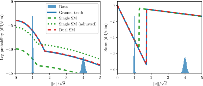
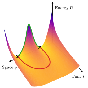
Figure 1: Comparison of single and dual score matching on recovering the energy of a scale mixture of two Gaussians in $d=1000$ dimensions. Left: Radial slices of the log probability. The single score matching estimate (green dashed curve) fails to recover the true energy (blue solid curve), even after global normalization (green dotted curve), while dual score matching (red dashed curve) succeeds. Middle: Radial components of the scores. Single score matching learns an accurate score over the support of the data (blue bar plot) but not outside of it. Right: Energy landscape across space and time (noise level) for a mixture of two Gaussians in one dimension. The direct path between the modes at $t=0$ crosses a large energy barrier (green curve), which is alleviated on a path that is not time-restricted (red curve).

Traditionally, energy models are defined in terms of a parametric function $U_{\theta}(x)$ that approximates the unnormalized log density over $x\in\mathbb{R}^{d}$: $p_{\theta}(x)=\frac{1}{Z_{\theta}}\mathrm{e}^{-U_{\theta}(x)}$, with a normalizing constant $Z_{\theta}=\int\mathrm{e}^{-U_{\theta}(x)}\mathrm{d}x$. The parameters $\theta$ are estimated by minimizing the expected negative log likelihood (NLL), $\mathbb{E}_{x}\mathopen{}\mathclose{{\left[-\log p_{\theta}(x)}}\right]=\mathbb{E}_{x}\mathopen{}\mathclose{{\left[U_{\theta}(x)}}\right]+\log Z_{\theta}$, which is equivalent to minimizing the KL divergence between $p_{\theta}(x)$ and the data distribution. The normalizing constant $Z_{\theta}$ plays a critical role in learning, representing the total energy over $\mathbb{R}^{d}$ which trades off against the energy of the data. But direct estimation (i.e., computing the integral) is typically intractable.

The normalization constant can be eliminated from the NLL by differentiating w.r.t. $x$, yielding a quantity known as the score: $-\nabla_{x}\log p_{\theta}(x)=\nabla_{x}U_{\theta}(x)$. As a result, a score model can be efficiently fitted to data via “score matching” (Hyvärinen and Dayan, 2005), which minimizes the Fisher (rather than KL) divergence between the model and the data. In the case of data corrupted by Gaussian white noise, this amounts to solving a denoising problem (Vincent, 2011; Raphan and Simoncelli, 2011). But this computational advantage comes at a statistical cost: a good approximation of the score does not always lead to a good model of the energy (Koehler et al., 2023), as we now illustrate. Consider the case of an equal mixture of two multivariate Gaussian distributions with zero mean and different variances $\sigma_{1}^{2}$ and $\sigma_{2}^{2}$. In high dimensions, this distribution concentrates near the two spheres of radius $\sigma_{1}\sqrt{d}$ and $\sigma_{2}\sqrt{d}$, leading to data scarcity in the rest of the space. We show in Figure˜1 energies estimated from samples by optimizing their gradient via (single) score matching. This fails to recover the true energy, even after adjusting a normalization constant. Indeed, estimating the energy difference between the two Gaussians requires a good estimation of the score along an integration path between them. If there is no data in-between modes to constrain the score, due to an energy barrier or concentration phenomena, this leads to inconsistent energy values.

Diffusion models expand on score matching by learning scores of data corrupted by white Gaussian noise for a range of different noise amplitudes, $\nabla_{y}U(y,t)$, with $y=x+\mathcal{N}(0,t\mathrm{Id})$. The evolution of the density $p(y|t)$ as $t$ increases is a diffusion process, and thus the corresponding energies increase in smoothness with $t$. This multiscale family of scores can be used to draw high-quality samples from $p(x)$ using a reverse diffusion algorithm, which follows a trajectory of partial denoising steps (Song and Ermon, 2019; Song et al., 2021a; Ho et al., 2020; Kadkhodaie and Simoncelli, 2020). In fact, the diffusion scores implicitly capture a density model of the data (Song et al., 2021b; Kingma and Welling, 2013): the relative energy levels between modes are encoded in the score at the time $t$ when they merge (Raya and Ambrogioni, 2023; Biroli et al., 2024). This density model can be evaluated in various ways, which all involve a tractable but costly integration of score divergences (or denoising errors) along time (Song et al., 2021a; Kong et al., 2023; Skreta et al., 2024; Karczewski et al., 2025). Intuitively, diffusion provides a high-probability path between modes through space and time, as visualized in Figure˜1. Energy differences along time can then be retrieved by integrating the “time score” $\partial_{t}U_{\theta}(y,t)$ (Choi et al., 2022), which is implicitly determined from the diffusion equation (Song et al., 2021a; Lai et al., 2023). See Section˜A.2 for a more in-depth exposition. Here, we propose to learn the “space-time” energy landscape directly by matching both space and time scores.

2.2 Dual score matching: Objective function

Space and time score matching.

We want to learn a time-dependent energy function, $U_{\theta}(y,t)$, to approximate the NLL of the noisy image distribution at all noise levels $t$:

$$U(y,t)=-\log\mathopen{}\mathclose{{\left(\int p(x)\mathrm{e}^{-\frac{1}{2t}\|x-y\|^{2}-\frac{d}{2}\log\mathopen{}\mathclose{{\left(2\pi t}}\right)}\mathrm{d}x}}\right).$$ (1)

Differentiating this NLL with respect to $y$ gives the “space score”, which can be expressed using the Miyasawa-Tweedie identity (Robbins, 1956; Miyasawa, 1961) as

$$\nabla_{y}U(y,t)=\mathbb{E}_{x}\mathopen{}\mathclose{{\left[\frac{y-x}{t}\,\middle|\,y}}\right].$$ (2)

It leads to the denoising score matching objective (Vincent, 2011; Raphan and Simoncelli, 2011) used to train diffusion models:

$$\ell_{\rm DSM}(\theta,t)=\mathbb{E}_{x,y}\mathopen{}\mathclose{{\left[{\mathopen{}\mathclose{{\left\lVert\nabla_{y}U_{\theta}(y,t)-\frac{y-x}{t}}}\right\rVert}^{2}}}\right].$$ (3)

We also can differentiate the energy with respect to $t$, producing a “time score”, for which we can derive a similar score-matching identity (see Section˜B.1):

$$\partial_{t}U(y,t)=\mathbb{E}_{x}\mathopen{}\mathclose{{\left[\frac{d}{2t}-\frac{{\mathopen{}\mathclose{{\left\lVert y-x}}\right\rVert}^{2}}{2t^{2}}\,\middle|\,y}}\right].$$ (4)

From this identity, we define an analogous “time score matching” objective:

$$\ell_{\rm TSM}(\theta,t)=\mathbb{E}_{x,y}\mathopen{}\mathclose{{\left[\mathopen{}\mathclose{{\left(\partial_{t}U_{\theta}(y,t)-\frac{d}{2t}+\frac{{\mathopen{}\mathclose{{\left\lVert y-x}}\right\rVert}^{2}}{2t^{2}}}}\right)^{2}}}\right].$$ (5)

Matching both scores enforces that the learned energy $U_{\theta}(y,t)$ is a solution of the diffusion equation, which is critical for combining information across noise levels into accurate energy values at $t=0$.

Combining objectives across noise levels.

The two objectives in eqs.˜3 and 5 are defined for a fixed noise level $t$. We can form an overall objective by integrating over $t$, with an appropriate weighting. For the denoising score matching objective, a natural choice is the so-called maximum-likelihood weighting (Song et al., 2021b; Kingma et al., 2021), which provides a bound on the KL divergence with the data distribution:

$$\operatorname{KL}\mathopen{}\mathclose{{\left(p\,\middle\|\,\tilde{p}_{\theta}}}\right)\leq\frac{1}{2}\int_{0}^{\infty}\ell_{\rm DSM}(\theta,t)\,\mathrm{d}t,$$ (6)

where $\tilde{p}_{\theta}$ is the implicit density of the generative diffusion model. This integral can be approximated by Monte-Carlo sampling from a distribution of noise levels. In practice, we have found it best to sample $\log t$ uniformly over a finite interval (specifically, $p(t)\propto 1/t,t\in[t_{\min},t_{\max}]$), which corresponds to the following implementation of the integral:

$$\int_{t_{\min}}^{t_{\max}}\ell_{\rm DSM}(\theta,t)\,\mathrm{d}t=\mathbb{E}_{t}\mathopen{}\mathclose{{\left[t\,\ell_{\rm DSM}(\theta,t)}}\right].$$ (7)

Appreciably, the resulting term in the expected value is unitless: it is invariant to a simultaneous rescaling of the data and noise level. We thus choose to weight the time score matching objective in eq.˜5 by $t^{2}$, so that it is also unitless, and to evaluate over the same distribution $p(t)$. Finally, after normalization by the dimensionality $d$, we simply add both objectives (we found no significant improvement from tuning a tradeoff hyperparameter). Our dual score matching objective is then

$$\ell(\theta) =\mathbb{E}_{t}\mathopen{}\mathclose{{\left[\frac{t}{d}\,\ell_{\rm DSM}(\theta,t)+\mathopen{}\mathclose{{\left(\frac{t}{d}}}\right)^{2}\,\ell_{\rm TSM}(\theta,t)}}\right].$$ (8)

Normalization.

The learned energy $U_{\theta}(y,t)$ is only estimated up to an additive constant, since the two objective functions only constrain its partial derivatives. An important aspect of our framework is that it enables estimation of this normalizing constant. Indeed, the time score objective ensures that this normalizing constant does not depend on time, as mass is conserved through the diffusion. This allows normalizing the model at the largest noise level $t_{\max}$, where the true distribution is almost Gaussian: $p(y|t_{\max})\approx\mathcal{N}(0,t_{\max}\mathrm{Id})$. We thus set the average energy value at $t=t_{\max}$ to the entropy of this Gaussian distribution:

$$U_{\theta}(y,t)\longrightarrow U_{\theta}(y,t)-\mathbb{E}_{y}\mathopen{}\mathclose{{\left[U_{\theta}(y,t)\,\middle|\,t=t_{\max}}}\right]+\frac{d}{2}\log(2\pi\mathrm{e}t_{\max}).$$ (9)

Figure˜1 verifies that dual score matching indeed provides both consistent and normalized energy values (in particular, for $t=0$), in contrast to single score matching. We note however that eq.˜9 is an approximate normalization procedure, which we discuss at more length in Section˜A.3.

2.3 Dual score matching: Architecture

How should one choose an architecture to compute the energy $U_{\theta}(y,t)$? Rather than designing one from scratch (Salimans and Ho, 2021; Cohen et al., 2021; Thiry and Guth, 2024), we instead construct one by modifying a score-based denoising architecture that is known to have appropriate inductive biases. Let $s_{\theta}\colon\mathbb{R}^{d}\times\mathbb{R}\to\mathbb{R}^{d}$ be such an architecture (e.g., a UNet). We wish to define a new architecture $U_{\theta}\colon\mathbb{R}^{d}\times\mathbb{R}\to\mathbb{R}$ such that $\nabla_{y}U_{\theta}\approx s_{\theta}$, preserving the inductive biases of $s_{\theta}$. We propose to set

$$U_{\theta}(y,t)=\frac{1}{2}\mathopen{}\mathclose{{\left\langle y,s_{\theta}(y,t)}}\right\rangle.$$ (10)

We show in Section˜B.2 that $\nabla_{y}U_{\theta}(y,t)=s_{\theta}(y,t)$ if the score network $s_{\theta}$ is conservative and homogeneous (Romano et al., 2017; Reehorst and Schniter, 2018). Homogeneity has been shown to hold approximately in the related setting of blind denoisers (Mohan* et al., 2020; Herbreteau et al., 2023). We note that the seemingly similar choice of a squared norm such as $U_{\theta}(y,t)=\frac{1}{2}{\mathopen{}\mathclose{{\left\lVert s_{\theta}(y,t)}}\right\rVert}^{2}$ used in some previous energy models (Salimans and Ho, 2021; Hurault et al., 2021; Du et al., 2023; Yadin et al., 2024; Thiry and Guth, 2024) leads to the same desirable homogeneity properties in $y$ but not in $\theta$, and thus fails to preserve the optimization properties of the original score network. We describe further architectural details in Section˜C.1.

2.4 Performance evaluation

Denoising performance.

We first verify that the gradient of the energy network $U_{\theta}$ provides as good a denoiser as the score network on which it is based, $s_{\theta}$. Both networks are separately trained; $U_{\theta}$ with the dual score matching objective (eq.˜8, using double back-propagation) and $s_{\theta}$ with only the standard (denoising) score matching objective (eq.˜3). Further details are provided in Section˜C.2. We compare their denoising performance across noise levels in Table˜1. For all but the smallest noise levels, the energy-based model achieves (slightly) better denoising performance than the score model. These results show that there is no penalty in modeling the energy rather than the score. This is contrary to the results of Salimans and Ho (2021), and is likely due to our use of an architecture that is homogeneous, and for which non-conservativeness of the score is not a large source of denoising error (Mohan* et al., 2020; Chao et al., 2023). Finally, these results also demonstrate that the two components of our dual score matching objective are not trading off against each other; rather, they complement and even reinforce each other.

Table 1: Denoising MSE at several noise levels for corresponding score and energy networks, averaged over images in ImageNet64. All quantities are expressed as peak signal-to-noise ratio (PSNR) in dB: $\mathrm{PSNR}=-10\log_{10}(\mathrm{MSE})$.

Noise variance	$90$	$75$	$60$	$45$	$30$	$15$	$0$	$-15$	$-30$
Score network	$\mathbf{90.20}$	$\mathbf{75.47}$	$60.43$	$47.19$	$35.58$	$25.92$	$18.84$	$13.31$	$-0.11$
Energy network	$90.09$	$75.17$	$\mathbf{60.45}$	$\mathbf{47.25}$	$\mathbf{35.67}$	$\mathbf{26.01}$	$\mathbf{18.88}$	$\mathbf{13.48}$	$\mathbf{\hphantom{-}2.53}$

Negative log likelihood.

How accurate are our energy estimates? A standard evaluation of probabilistic models consists of calculating the cross-entropy $\mathbb{E}_{x}\mathopen{}\mathclose{{\left[-\log p_{\theta}(x)}}\right]$ between the data distribution and the model, also known as negative log likelihood (NLL). In practice, NLL computes how much probability the model assigns to a held-out test set. There are however several subtleties that make direct comparisons challenging. Specifically, there are 3 factors that can cause variations in NLL up to $\pm 0.5$ bits/dimension or more: details of data pre-processing (e.g., downsampling or data augmentation), conversion method from continuous to discrete probabilities, and the estimator type (exactly normalized, variational bound, or approximately normalized). We expand on these issues in Section˜A.1.

We compare NLLs of our method and a variety of recent energy models in Table˜2. This evaluation demonstrates that our model is comparable to the best-performing models in the literature, within the variability arising from the three factors of variation mentioned in the previous paragraph. Two unique advantages of our method are that it provides (1) direct (one-shot) estimates of energy (as opposed to other density estimation approaches in diffusion models, which we review in Section˜A.2), greatly facilitating analysis, and (2) access to energy across all noise levels, providing a window into larger-scale features of the energy landscape.

Table 2: Negative log likelihood (in bits/dimension) on ImageNet64 test set. See Section˜A.1 for more details.

Method	Anti-aliasing	Augmentation	Discreteness	Type	Single NFE	NLL
Glow (Kingma and Dhariwal, 2018)	✗	None	Continuous	Normalized	✓	3.81
PixelCNN (Van den Oord et al., 2016)	✗	None	Discrete	Normalized	✗	3.57
I-DDPM (Nichol and Dhariwal, 2021)	✗	None	Continuous	Upper bound	✗	3.54
VDM (Kingma et al., 2021)	✗	None	Discrete	Upper bound	✗	3.40
FM (Lipman et al., 2023)	✓	None	Uniform*	Normalized	✗	3.31
NFDM (Bartosh et al., 2024)	✗	Horizontal flips	Uniform*	Normalized	✗	3.20
TarFlow (Zhai et al., 2024)	✗	Horizontal flips	Uniform	Normalized	✓	2.99
Ours	✓	Horizontal flips	Continuous	Estimate	✓	3.36

3 Analysis of the learned energy-based model

3.1 Generalization

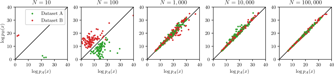
Figure 2: Convergence of energy estimates. The data set is split into two halves (denoted A and B), and separate energy models are trained on $N$ samples drawn from each half. Each scatterplot compares the $\log p(x)$ estimated by the two models at $t=0$ over all $2N$ training images. As $N$ increases, the energy estimates of the two models converges for all images.

The previous section demonstrated that our energy-based model achieves near state-of-the-art NLL on ImageNet64. That is, the model on average assigns high probability to a set of held-out images. Next, we establish that the energies of the individual images are reliable. In particular, we require that the model’s energy assignment is stable under change of the training data.

To this end, we borrow the strong generalization test developed in Kadkhodaie et al. (2024). We partition the training data into two non-overlapping sets, train a separate energy-based model on each set, and then compare the energies computed by these two models on their own and each other’s training examples. We gradually increase the size of each training set until the two models assign approximately equal log probability across all images. Figure˜2 shows the results of this experiment. The two models assign very different probabilities to the same image when the training set size, $N$, is small. But they converge gradually and compute almost the same values at $N=10^{5}$. Note that the rate of convergence depends on the probability: more data is needed before the two models agree on the high-probability images. It is also worth noting that the transition from memorization to generalization of energy models is marked by a large increase of variance in energy over the training set (starting at $N=100$).

This result establishes that the model variance vanishes with a feasible training set size, demonstrating lack of memorization. However, it does not guarantee that the values are accurate, as the models could be biased. Calculating model bias is not possible without access to the true density, hence it can only be obtained for simple analytical models (as in Figure˜1). However, smaller NLL values over test data (Table˜2) are indicative of a smaller model bias.

3.2 Distribution of energies and relationship to image content

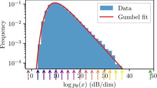
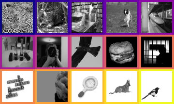
Figure 3: Histogram of log probabilities of images in the ImageNet dataset. Color-coded arrows indicate values for the example images on the right, and the leftmost (brown) and rightmost (green) arrows indicate values for a uniform noise image in $[0,1]$ and a constant image of intensity $0.5$, respectively. The distribution is well-fit by a Gumbel distribution (red line). Additional examples of images organized by probability are shown in Figures˜6, 7 and 8 (Appendix˜D).

We now study properties of the learned energy model. What is the entropy (average energy) of the image dataset? Do all images have the same probability? If not, what determines the probability of an image? To investigate these questions, we compute the log probability of all $50,000$ images in the ImageNet test set in Figure˜3. We express log probability in units of decibels per dimension (dB/dim), computed as $\frac{1}{d}10\log_{10}p_{\theta}(x)$. In this scale, an additive change of $10$ dB/dim corresponds to a multiplicative change in probability density of $10^{d}$.

Entropy.

The average of $-\log p_{\theta}(x)$ provides an estimate of the differential entropy of ImageNet, which is here equal to $-11.4$ dB/dim. Note that the uniform distribution over the hypercube $[0,1]^{d}$ has an entropy of $0$. This indicates that natural images occupy a fractional volume of about $10^{-1.14d}$. This can be converted to an estimate of discrete entropy by assuming that log probability is constant within quantization bins. For $256$ possible intensity values ($8$ bits), this gives an entropy of $4.20$ bits/dimension (the difference with Table˜2 comes from the use of grayscale images here). In other words, there are $\sim 10^{5,180}$ quantized ImageNet images out of $10^{9,860}$ possible images at this resolution.

Lack of concentration.

Many high-dimensional probability distributions exhibit a concentration phenomenon, where typical realizations have nearly equal energy. For instance, in simple image probability models such as a Gaussian model or a sparse wavelet model (where wavelet coefficients are independent), the energy of independent components add, and the law of large numbers imply a concentration of the energy around its mean. In contrast, our energy network reveals enormous diversity in the log probabilities of individual ImageNet images (Figure˜3). Over the entire test set, they span a range of $34.4$ dB/dim, corresponding to a probability ratio of $\approx 10^{14,000}$. To make sense of this value, it is important to realize that the frequency of images with a given value of $\log p$ in a dataset is equal to this probability value multiplied by the volume of the corresponding probability level set. Observing a range of probability values of $10^{14,000}$ thus reveals that these enormous variations in probability density are nearly compensated by inverse variations in the volume of their corresponding level sets.

Shape of the distribution of log probabilities.

The distribution of log probabilities values is highly skewed: there is a heavy tail of high-probability images and a much lighter tail of low-probability images. Surprisingly, this distribution is well approximated by a Gumbel distribution (we report parameter values in Section˜C.3). It arises as a limit distribution for the maximum of many i.i.d. random variables. This surprising observation is, to the best of our knowledge, new, and calls for an explanation. In independent component models, the log probabilities are sums of i.i.d. random variables, and are therefore Gaussian distributed (with a vanishing variance compared to their mean). A simple model which reproduces this Gumbel distribution is a high-dimensional spherically-symmetric distribution with an exponentially-distributed radial marginal.

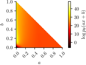
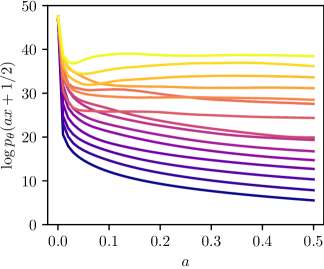
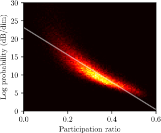
Figure 4: Influence of image statistics on probability. Left. $\log p_{\theta}(ax+b)$ as a function of $a$ and $b$. Middle. Horizontal slice ($b=\frac{1}{2}$) of the left plot for the example images of Figure˜3. Right. Log probability as a function of sparsity, measured as the participation ratio of wavelet coefficients.

Image content.

We also show in Figure˜3 examples of images at various log probabilities. High-probability images invariably contain small (often high-contrast) objects, on a blank (often white) background. Conversely, low-probability images are generally filled with dense detailed texture. This agrees with the behavior of compression engines. Indeed, the energy of an image, when expressed in bits, corresponds to the size of its optimally compressed representation. This implies that low-probability images should intuitively have more “content” than high-probability images.

Intensity range and sparsity.

Following these visual observations, we further examine the influence of intensity range and sparsity on image probability (Figure˜4). First, we evaluate the log probability of reference images as we manipulate their brightness or contrast through an affine operation. We find that the brightness has minimal effect on the probability, while higher-contrast images have lower probability. This reveals that the distribution is star-shaped: any pair of images are connected by a high-probability path passing through a constant image. Next, we verify that log probability is correlated with a simple measure of sparsity of images. We compute a multi-scale wavelet decomposition of the images, and measure the $\ell^{1}$-norm divided by the $\ell^{2}$-norm of the coefficients. The square of this quantity, $\|x\|_{1}^{2}/d\|x\|^{2}_{2}\in(0,1]$ is known as participation ratio, with smaller values indicating higher sparsity. The right panel of Figure˜4 shows that this simple measure is indeed predictive of $\log p_{\theta}(x)$ (albeit not very precisely).

3.3 Effective dimensionality of the energy landscape

Beyond estimating log probability for a given image, we aim to characterize the local behavior of the density in the vicinity of that image. For instance, we would like to assess whether the probability is locally concentrated near a low-dimensional “tangent” subspace, and if so, estimate its dimensionality. In this section, we explain how these quantities may be computed from our energy model. We then show that the local dimensionality around an image is often much lower than the ambient dimensionality of the space, but that this dimensionality varies with the particular image and the scale that is used to define the local neighborhood.

Multi-scale dimensionality.

Consider the distribution supported on the blue regions in the left two panels of Figure˜5. For the leftmost region, the effective dimensionality of a local neighborhood decreases with the size of that neighborhood. The opposite behavior is also possible, as shown in the rightmost region. These examples show that dimensionality measures which aim to describe these geometrical structures need to depend on both the location and the scale of the neighborhood (Tempczyk et al., 2022).

Effective dimensionality.

We now introduce an effective dimensionality measure which can be equivalently defined from the optimal denoiser or the evolution of the probability landscape as it diffuses. Given a noisy observation $y$ of a clean image $x$ with noise variance $t$, the optimal denoiser estimates $x$ with the conditional expectation $\mathbb{E}\mathopen{}\mathclose{{\left[x\,\middle|\,y}}\right]$. Its average deviation from $x$ capture the local support of the data distribution around $x$ at scale $t$. Intuitively, from observing $y$, the optimal denoiser identifies that $x$ is located on a $d_{\rm eff}$-dimensional “tangent” space and projects $y$ onto it. This preserves the components of the noise that lie along the subspace, incurring a denoising error $td_{\rm eff}$. Thus, we define the local effective dimensionality around $x$ at scale $t$ as

$$d_{\rm eff}(x,t)=\frac{1}{t}\mathbb{E}_{y}\mathopen{}\mathclose{{\left[{\mathopen{}\mathclose{{\left\lVert x-\mathbb{E}_{x}\mathopen{}\mathclose{{\left[x\,\middle|\,y}}\right]}}\right\rVert}^{2}\,\middle|\,x}}\right].$$ (11)

Effective dimensionality can be equivalently defined directly from the energy. Consider the forward diffusion which progressively adds more noise to an image $x$, blurring the probability landscape. At time $t$, we can define an effective energy $\mathbb{E}_{y}\mathopen{}\mathclose{{\left[U(y,t)\,\middle|\,x}}\right]$. Its rate of change with $t$ captures the effective dimensionality around $x$. Intuitively, if this landscape is locally a $d_{\rm eff}$-dimensional subspace, then adding more noise causes probability to diffuse in the $d-d_{\rm eff}$ normal “off-manifold” directions, spreading over a volume $\sim t^{(d-d_{\rm eff})/2}$. Taking the logarithm, we obtain $\mathbb{E}_{y}\mathopen{}\mathclose{{\left[U(y,t)\,\middle|\,x}}\right]\sim(d-d_{\rm eff})\frac{1}{2}\log t$. Thus, we can equivalently define

$$d_{\rm eff}(x,t)=d-\partial_{\frac{1}{2}\log t}\mathbb{E}_{y}\mathopen{}\mathclose{{\left[U(y,t)\,\middle|\,x}}\right].$$ (12)

We show in Section˜B.3 that the definitions in eqs.˜11 and 12 are equivalent, unifying two seemingly distinct points of views adopted in related dimensionality measures (Wu and Verdú, 2011; Mohan* et al., 2020; Tempczyk et al., 2022; Stanczuk et al., 2022; Kamkari et al., 2024; Horvat and Pfister, 2024).

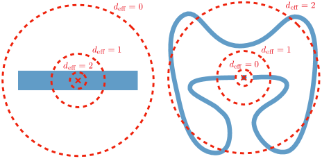
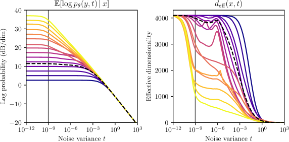
Figure 5: Left: Two hypothetical examples illustrating how local effective dimensionality depends on the scale of the neighborhood. For both examples, support of density corresponds to the blue regions. In the left example, the dimensionality around the red point decreases with scale (from 2 down to 0), while the opposite is true for the right example. Right: Log probability and effective dimensionality as a function of noise level. Colored lines correspond to different example images $x$ (shown in right panel of Figure˜3), while the dashed black line shows the average over the ImageNet test set. The vertical gray line indicates the minimum noise level presented during training ($t=10^{-9})$, and the horizontal gray line the ambient dimensionality of the dataset ($d=4096$).

Numerical results.

We show in Figure˜5 the behavior of the effective energy and dimensionality as a function of the noise level. As the noise level increases, the log probability initially remains constant, indicating that probability is uniformly spread in a ball around $x$. The probability eventually decreases as the diffusion radius becomes larger than the local support size, and all lines converge to the mean (the negative entropy), consistent with the asymptotic Gaussian behavior of the energy. The effective dimensionality vanishes at large noise levels (images have a compact support, which eventually looks like a point at large enough scales) but increases as the noise level is reduced, eventually reaching the ambient dimensionality $d$ (our model has a continuous non-zero density everywhere by construction). In-between these two extremes, there exists a sizable range of scales $t\in[{10}^{-9},{10}^{-2}]$ where almost the entire range of dimensionalities coexist. In particular, higher-probability images have lower-dimensional neighborhoods, even at relatively small scales, while lower-probability images have nearly full-dimensional neighborhoods, even at relatively large scales. We note two potential limits to these estimates. First, the quantization of pixel values into bins of size $1/256$ limits the resolution to $t\sim{10}^{-5}$, possibly explaining the momentary decrease in dimensionality as $t$ decreases. Second, our energy model was only trained on noise levels down to $t_{\min}={10}^{-9}$. Thus, energies at smaller values of $t$ are solely determined by model inductive biases, which favor a constant energy.

4 Discussion

We have developed a novel framework for estimating the log probability (energy) of a distribution of images from observed samples. The estimation method is simple and robust, and converges to a stable solution with relatively small amounts of data (in our examples, $100,000$ images of size $64\times 64$ suffices). The framework leverages the tremendous power of generative diffusion models, relying on networks trained to estimate the score of the data distribution by minimizing a denoising objective. We augment this with a secondary objective that ensures consistency of the model across noise levels, and an architecture constructed from an existing denoiser so as to preserve its inductive biases. We validate our model by verifying that it achieves denoising performance equal to or surpassing the original denoiser, and NLL values comparable to the state of the art.

We have investigated the geometrical properties of the learned energy model. Notably, we observe a lack of concentration of measure, with log probability values varying over a wide range and following a Gumbel distribution. As a limit distribution for the maximum, rather than the sum, of i.i.d. random variables, we expect that this might arise in a broad class of high-dimensional probability distributions. We also introduced a novel image- and scale-dependent effective dimensionality measure which unifies two separate points of view adopted in the literature. We demonstrate that different image neighborhoods display both high and low dimensionality over a wide range of scales. These results challenge simple interpretations of the manifold hypothesis. Furthermore, the estimated dimensionalities remain too high to explain how the curse of dimensionality may be lifted. This indicates that the energy landscape of natural images must have additional geometrical regularity.

Limitations

We mention two main limitations of our work. First, our energy model has a roughly doubled training time compared to the base score network, due to the use of double back-propagation. We believe this can be improved through architecture improvements or specialized auto-differentiation functions. Another limitation of our approach is that we cannot provide any theoretical guarantees that minimizing our objective leads to a quantitative approximation of the energy (see Section˜A.3).

Appendix A Discussions on density estimation

A.1 On comparison of NLL values

We identify three issues that arise in estimation of NLL values, each of which limits the precision with which they can be compared.

A first issue concerns the selection and pre-processing of the training data. There are two different versions of ImageNet at $64\times 64$ resolution: one introduced in Van den Oord et al. [2016], no longer available, and a second which uses anti-aliasing during downsampling (reducing entropy and thus NLL), introduced in Chrabaszcz et al. [2017]. This change in the dataset accounts for variations of about 0.3 bits/dimension [Zheng et al., 2023]. Similarly, the data augmentations used can both increase entropy (e.g., random flips) or reduce it (e.g., center crops, or resizing operations with anti-aliasing).

A second point is that NLL estimates must be computed on a discrete probability model, and NLL estimates for continuous models are dependent on the method used to discretize the distribution. The simplest option is to assume that the probability is uniform within quantization bins. Discrete probabilities are then computed as a product of the continuous probability with the volume of the quantization bin, which corresponds to an additive shift of 8 bits in the NLL for image data. This can be enforced by adding uniform noise to the data, a technique known as “uniform dequantization” [Ho et al., 2019], which leads to an upper bound on the NLL of the corresponding discrete model [Theis et al., 2016]. These differences can account for variations of 0.1 to 0.5 bits/dimension [Kong et al., 2023]. A more sophisticated variational dequantization procedure can improve results by an additional 0.1 bits/dimension [Ho et al., 2019, Song et al., 2021b]. In contrast, directly modeling the discrete data with appropriate methods can lead to reductions in NLL of more than 2 bits/dimension [Bhattacharya et al., 2025].

Finally, a third point is that depending on the method, the NLL should be interpreted differently. Classically, $p_{\theta}$ is a normalized probability distribution, typically obtained through a change-of-variable formula (as in flow-based models), so that up to an unknown additive constant (the entropy of the data), the NLL directly evaluates the KL divergence $\operatorname{KL}\mathopen{}\mathclose{{\left(p\,\middle\|\,p_{\theta}}}\right)$. For some other models (such as VAEs), the NLL is not directly tied to a probabilistic model and is instead evaluated through a variational lower bound, leading to upper bounds on $-\log p(x)$ for each $x$. The NLL however remains an upper bound on the entropy of the data. The MSE-based formulas of Kong et al. [2023] also fall in this category when using a (necessarily suboptimal) network denoiser. Lastly, approximately normalized energy-based models such as ours or CDM [Yadin et al., 2024] compute estimates of $-\log p(x)$ that are neither lower nor upper bounds, so that NLL can only be interpreted as an estimate of the entropy of the data.

As a result of these differences, NLL values of different methods are often not directly comparable. Here, we aim to learn an accurate continuous probability model of image distributions rather than obtaining the best upper bound on the discrete entropy of the data.

When evaluating previously published NLL results, we found that these details were often not provided, and we thus had to make assumptions in compiling Table˜2. The “anti-aliasing” column refers to the version of ImageNet64 used, we assumed that articles that cite Van den Oord et al. [2016] for the dataset made use of the aliased version. We assume no data augmentation if none is mentioned (for TarFlow [Zhai et al., 2024], the authors mention performing center crops of the data, but an inspection of their code indicates that it has been disabled for ImageNet64). The “discreteness” column refers to the nature of the probability model and the potential conversion from continuous to discrete probabilities (“discrete” for discrete probability models, “continuous” for an additive shift of $8$ bits, and “uniform” for uniform dequantization by adding uniform noise). We assume a continuous model if no dequantization is mentioned (FM [Lipman et al., 2023] and NFDM [Bartosh et al., 2024] use a slightly different notion of uniform dequantization which improves NLL by 0.04 bits/dimension). The “type” column refers to the nature of the LLM estimate (“normalized” for an exactly normalized probability model coming from a flow-based model, “upper bound” for variational lower bounds on log probability, and “estimate” for other approaches). Finally, we indicate those methods that use a single neural function evaluation (NFE) to compute log probability in the “single NFE” column.

A.2 Background on density computation in diffusion models

We review several methods of estimating log probabilities from diffusion models that have appeared in the literature.

In early publications on diffusion methods, probabilities are computed with the so-called probability flow ODE [Song et al., 2021a]. This corresponds to the distribution of samples generated by the backward ODE. Given a large noise level $t_{\max}$, the backward ODE solves the equation

$$-\frac{\mathrm{d}x_{t}}{\mathrm{d}t}=-\frac{1}{2}\nabla_{y}U_{\theta}(x_{t},t),$$ (13)

backwards in time from $x_{t_{\max}}\sim\mathcal{N}(0,t_{\max}\mathrm{Id})$ and produces an approximate sample $x=x_{0}\sim p_{\rm ODE}$. The log probability of this sample can be calculated as [Song et al., 2021a]

$$-\log p_{\rm ODE}(x)=\frac{{\mathopen{}\mathclose{{\left\lVert x_{t_{\max}}}}\right\rVert}^{2}}{2t_{\max}}+\frac{d}{2}\log\mathopen{}\mathclose{{\left(2\pi t_{\max}}}\right)-\frac{1}{2}\int_{0}^{t_{\max}}\Delta_{y}U_{\theta}(x_{t},t)\mathrm{d}t.$$ (14)

Note that eq.˜14 is also valid for arbitrary test points $x$, in which case the ODE (13) needs to be solved forward in time from $x_{0}=x$ at $t=0$ to $t=t_{\max}$. Equation˜14 requires estimating the divergence of the score (the Laplacian of the energy), which is typically approximated with the Hutchinson trace estimator [Hutchinson, 1989].

Another approach is to use a variational bound as in Song et al. [2021b], Kingma et al. [2021], Kong et al. [2023]. This variational bound arises from the exact identity [Kong et al., 2023]

$$-\log p(x)=\mathbb{E}_{y}\mathopen{}\mathclose{{\left[U(y,t_{\max})\,\middle|\,x}}\right]-\int_{0}^{t_{\max}}\mathopen{}\mathclose{{\left(td-\mathbb{E}_{y}\mathopen{}\mathclose{{\left[{\mathopen{}\mathclose{{\left\lVert x-\mathbb{E}_{x}\mathopen{}\mathclose{{\left[x\,\middle|\,y}}\right]}}\right\rVert}^{2}\,\middle|\,x}}\right]}}\right)\frac{\mathrm{d}t}{2t^{2}}.$$ (15)

The first term is the effective energy at $t=t_{\max}$, which is equivalent to $\frac{d}{2}\log\mathopen{}\mathclose{{\left(2\pi\mathrm{e}t_{\max}}}\right)$ as $t_{\max}\to\infty$. The second term features the optimal mean squared error over noise levels $t\in[0,t_{\max}]$. Note that the integrand can be rewritten as $(d-d_{\rm eff}(x,t))\mathrm{d}\mathopen{}\mathclose{{\left(\frac{1}{2}\log t}}\right)$, and eq.˜15 can thus be derived by integrating the two equivalent definitions of effective dimensionality (11) and (12) (see Section˜B.3). Equation˜15 naturally leads to an upper-bound on the negative log probability of the data when replacing the optimal denoiser $\mathbb{E}_{x}\mathopen{}\mathclose{{\left[x\,\middle|\,y,t}}\right]$ with the denoiser derived from the Miyasawa-Tweedie expression, $y-t\nabla_{y}U_{\theta}(y,t)$:

$$-\log p_{\rm MSE}(x)=\frac{d}{2}\log\mathopen{}\mathclose{{\left(2\pi\mathrm{e}t_{\max}}}\right)-\int_{0}^{t_{\max}}\mathopen{}\mathclose{{\left(td-\mathbb{E}_{y}\mathopen{}\mathclose{{\left[{\mathopen{}\mathclose{{\left\lVert x-y+t\nabla_{y}U_{\theta}(y,t)}}\right\rVert}^{2}\,\middle|\,x}}\right]}}\right)\frac{\mathrm{d}t}{2t^{2}}.$$ (16)

This framework can be generalized to other noise distributions [Guo et al., 2013] such as Poisson noise, which is more adapted to discrete distributions [Bhattacharya et al., 2025].

Finally, it was recently observed in Skreta et al. [2024], Karczewski et al. [2025] that a cheaper unbiased stochastic estimator of this bound can be obtained with the Itô formula. Given a realization $(x_{t})_{t\in\mathbb{R}_{+}}$ of the forward SDE (Brownian motion) $\mathrm{d}x_{t}=\mathrm{d}w_{t}$ started at $x_{0}=x\sim p(x)$, then

$$-\log p(x)=U(x_{t_{\max}},t_{\max})-\int_{0}^{t_{\max}}\mathopen{}\mathclose{{\left(\mathopen{}\mathclose{{\left\langle\nabla_{y}U(x_{t},t),\mathrm{d}x_{t}}}\right\rangle-\frac{1}{2}{\mathopen{}\mathclose{{\left\lVert\nabla_{y}U(x_{t},t)}}\right\rVert}^{2}\mathrm{d}t}}\right).$$ (17)

When $t_{\max}\to\infty$, one can again use $U(x_{t_{\max}},t_{\max})\sim\frac{{\mathopen{}\mathclose{{\left\lVert x_{t_{\max}}}}\right\rVert}^{2}}{2t_{\max}}+\frac{d}{2}\log\mathopen{}\mathclose{{\left(2\pi t_{\max}}}\right)$. Replacing the unknown true energy $U$ in the integrand with a model $U_{\theta}$ leads to a biased stochastic estimate of the log probability:

$$-\log p_{\rm SDE}(x)=\frac{{\mathopen{}\mathclose{{\left\lVert x_{t_{\max}}}}\right\rVert}^{2}}{2t_{\max}}+\frac{d}{2}\log\mathopen{}\mathclose{{\left(2\pi t_{\max}}}\right)-\int_{0}^{t_{\max}}\mathopen{}\mathclose{{\left(\mathopen{}\mathclose{{\left\langle\nabla_{y}U_{\theta}(x_{t},t),\mathrm{d}x_{t}}}\right\rangle-\frac{1}{2}{\mathopen{}\mathclose{{\left\lVert\nabla_{y}U_{\theta}(x_{t},t)}}\right\rVert}^{2}\mathrm{d}t}}\right).$$ (18)

Karczewski et al. [2025] show that averaging over SDE trajectories started at the same $x_{0}=x$ leads to an upper bound on the NLL, in fact recovering the one in eq.˜16.

In summary, the ODE gives deterministic probabilities exactly corresponding to the corresponding generative model (eq.˜14), while for the SDE one can choose between an denoising-based upper bound (eq.˜16) or a cheap stochastic estimator of it (eq.˜18). These evidently similar approaches are equivalent if and only if the model is consistent across noise levels (i.e., satisfies the diffusion equation). In practice, the choice of estimation method can lead to variations of up to 0.5 bits/dimension [Kong et al., 2023], see in particular Karczewski et al. [2025] for a careful study). These approaches also apply to our model, in addition to the direct evaluation of $U_{\theta}(x,t=0)$. While this latter estimate does not correspond to a generative model (like the ODE) or a variational bound (like the SDE), its main advantage is its computational efficiency, as it does not require integrating over noise levels and gives deterministic values without averaging over noise realizations (for a divergence term or mean squared error). We note the related work of Yadin et al. [2024] which also trains an energy model with score matching and a second objective. The main conceptual difference with our approach is that we use a continuous (as opposed to discrete) time variable $t$, which offerws robustness to noise level scheduling issues and to relies on the inductive biases of existing diffusion architectures (Section˜2.3).

A.3 On the theoretical justification of dual score matching

A limitation of our approach is that we offer no theoretical guarantees that minimizing our objective leads to a good approximation of the energy. It would be desirable to show that our training objective (assuming infinite training data) quantitatively controls the distance between the learned energy and the data energy. This could be achieved by showing that the joint distribution $p(y,t)$ (with $\log t$ uniformly distributed in $[\log t_{\min},\log t_{\max}]$) satisfies a Poincaré inequality, i.e.,

$$\mathrm{Var}\mathopen{}\mathclose{{\left[U_{\theta}(y,t)-U(y,t)}}\right]\leq C\mathbb{E}\mathopen{}\mathclose{{\left[{\mathopen{}\mathclose{{\left\lVert\nabla_{y}U_{\theta}(y,t)-\nabla_{y}U(y,t)}}\right\rVert}^{2}+(\partial_{t}U_{\theta}(y,t)-\partial_{t}U(y,t))^{2}}}\right],$$ (19)

for some constant $C$ that is not too large. While we conjecture that such a result holds (or a variant, such as when considering the distribution of $(y/\sqrt{t},\log t)$, to match our noise level weighting), note that this is weaker than a control in the Kullback-Leibler divergence. Replacing $\mathrm{Var}\mathopen{}\mathclose{{\left[U_{\theta}(y,t)-U(y,t)}}\right]$ with $\operatorname{KL}\mathopen{}\mathclose{{\left(p\,\middle\|\,p_{\theta}}}\right)$ in eq.˜19 would require that the model distribution $p_{\theta}(y,t)$ satisfies a log-Sobolev inequality, which could only be enforced with specific architectures. As a result, there is no control of the learned energy outside the support of the data distribution, so that out-of-distribution detection may be unreliable. It also implies our model may not be exactly normalized. Our NLL calculations are thus only approximate (although computationally cheap). These limitations are common to all current score-based and unnormalized energy-based approaches, including the related work of Yadin et al. [2024].

A.4 On frequency estimation with density models

Here, we describe a counter-intuitive property of density models in high dimensions which poses a challenge for estimating frequencies. We also refer the interested reader to Theis et al. [2016] which offers related observations.

Consider a mixture of two uniform distributions on two compact sets (classes) $C_{1}$ and $C_{2}$ with respective frequencies $f_{1}$ and $f_{2}$. The probability density is then constant on each class, with value $p_{i}=\frac{f_{i}}{V_{i}}$ where $V_{i}$ is the volume of $C_{i}$. The volume $V_{i}$ typically scales exponentially with $d$, $V_{i}\sim r_{i}^{d}$ where $r_{i}$ is the characteristic size of $C_{i}$. The energy values on each class are then

$$U_{i}=-\log p_{i}=d\log r_{i}-\log f_{i}.$$ (20)

In high dimensions $d\gg 1$, the energy values are dominated by the volume and only weakly depend on the frequencies of each class.

A concrete example of this phenomenon can be seen in the mixture of two Gaussian distributions considered in Figure˜1, where the two classes correspond to the two spheres of radius $\sqrt{d}\sigma_{i}$ for $i\in\{1,2\}$. The typical values of the energy $U_{i}=\frac{d}{2}\log\mathopen{}\mathclose{{\left(2\pi\mathrm{e}\sigma_{i}^{2}}}\right)-\log f_{i}$ are dominated by the entropy of the corresponding Gaussian. The energy is then determined by the value of the standard deviation $\sigma_{i}$ much more than the frequency $f_{i}$.

The implications of this observation for high-dimensional density models are twofold. First, estimated densities are dominated by volumes of typical sets (entropies of the mixture components), more than frequencies of different categories (one-dimensional marginals). The latter is easily learned from data, while estimating the former is a much more challenging task. Second, estimating energy up to a small relative error is not sufficient to capture observed frequencies. For our ImageNet64 model ($d=4096$), a relative error of $\sim 0.1$ dB/dimension (as estimated from the generalization experiment in Figure˜2) is negligible compared to typical energy differences of $\sim 10$ dB/dimension, but the required precision to estimate frequencies with a relative accuracy of $10\%$ is $1/d=2\times{10}^{-4}$ dB/dimension.

Appendix B Proofs and derivations

B.1 Time score matching (proof of eq.˜4)

We start from the expression of the energy (negative log probability) of noisy data:

$$U(y,t) =-\log p(y|t),$$ (21)

$$p(y|t) =\int p(x)p(y|x,t)\mathrm{d}x.$$ (22)

Differentiating the energy with respect to $t$ yields

$$\partial_{t}U(y,t) =-\frac{\partial_{t}p(y|t)}{p(y|t)}$$ (23)

$$=-\frac{\int p(x)p(y|x,t)\partial_{t}\log p(y|x,t)\mathrm{d}x}{p(y|t)}$$ (24)

$$=\mathbb{E}_{x}\mathopen{}\mathclose{{\left[-\partial_{t}\log p(y|x,t)\,\middle|\,y,t}}\right].$$ (25)

Note that the derivation exactly matches that of the Miyasawa-Tweedie identity by replacing $\partial_{t}$ with $\nabla_{y}$, and does not make any assumptions about the form of $p(y|x,t)$. Restricting to additive Gaussian noise, $-\log p(y|x,t)=\frac{1}{2t}{\mathopen{}\mathclose{{\left\lVert y-x}}\right\rVert}^{2}+\frac{d}{2}\log(2\pi t)$, and substituting into eq.˜25 gives the “time score-matching identity of eq.˜4:

$$\partial_{t}U(y,t)=\mathbb{E}_{x}\mathopen{}\mathclose{{\left[\frac{d}{2t}-\frac{{\mathopen{}\mathclose{{\left\lVert y-x}}\right\rVert}^{2}}{2t^{2}}\,\middle|\,y}}\right].$$ (26)

B.2 Energy architecture

Suppose that the energy network is defined in terms of a score network $s_{\theta}(y,t)$ as $U_{\theta}(y,t)=\frac{1}{2}\mathopen{}\mathclose{{\left\langle y,s_{\theta}(y,t)}}\right\rangle$, where the score network is assumed conservative and homogeneous. Conservativity means that there exists a scalar function $\phi$ such that $s_{\theta}(y,t)=\nabla_{y}\phi(y,t)$, which implies that the Jacobian $\nabla_{y}s_{\theta}(y,t)=\nabla^{2}_{y}\phi(y,t)$ is symmetric. The homogeneity property requires that for all $\lambda\geq 0$, $s_{\theta}(\lambda y,t)=\lambda s_{\theta}(y,t)$. Differentiating with respect to $\lambda$ and setting $\lambda=1$ yields

$$\nabla_{y}s_{\theta}(y,t)y=s_{\theta}(y,t).$$ (27)

We now calculate the gradient of the energy network:

$$\nabla_{y}U_{\theta}(y,t)=\frac{1}{2}\mathopen{}\mathclose{{\left(s_{\theta}(y,t)+\nabla_{y}s_{\theta}(y,t)^{\mathrm{T}}y}}\right)=s_{\theta}(y,t),$$ (28)

using the conservative and homogeneity properties to derive that $\nabla_{y}s_{\theta}(y,t)y=\nabla_{y}s_{\theta}(y,t)^{\mathrm{T}}y=s_{\theta}(y,t)$. Note that even if $s_{\theta}$ is not conservative, then it still holds that $\nabla_{y}U_{\theta}(y,t)=\frac{1}{2}\mathopen{}\mathclose{{\left(\nabla_{y}s_{\theta}(y,t)+\nabla_{y}s_{\theta}(y,t)^{\mathrm{T}}}}\right)y$, which can be interpreted as a symmetrization of the Jacobian of $s_{\theta}$.

We remark that if $s_{\theta}$ is homogeneous, then $U_{\theta}$ is quadratically homogeneous ($U_{\theta}(\lambda y,t)=\lambda^{2}U_{\theta}(y,t)$). Note that this does not correspond to enforcing (asymmetric) Gaussian one-dimensional marginals $\langle y,u\rangle$. Rather, this enforces that the distribution of $\langle y,u\rangle$ conditioned on the orthogonal projection $y-\langle y,u\rangle u/{\mathopen{}\mathclose{{\left\lVert u}}\right\rVert}^{2}$ is (asymmetric) Gaussian.

B.3 Effective dimensionality (equivalence between eqs.˜11 and 12)

We start by calculating the time derivative of the effective energy $\mathbb{E}_{y}\mathopen{}\mathclose{{\left[U(y,t)\,\middle|\,x}}\right]$. We have

$$\partial_{t}\mathbb{E}_{y}\mathopen{}\mathclose{{\left[U(y,t)\,\middle|\,x}}\right] =\partial_{t}\int p(y|x,t)U(y,t)\mathrm{d}y$$ (29)

$$=\int\mathopen{}\mathclose{{\left(\partial_{t}p(y|x,t)U(y,t)+p(y|x,t)\partial_{t}U(y,t)}}\right)\mathrm{d}y.$$ (30)

The first term is the derivative with respect to variance of a Gaussian distribution $\mathcal{N}(x,t\mathrm{Id})$. It satisfies the diffusion equation:

$$\partial_{t}p(y|x,t)=\frac{1}{2}\Delta_{y}p(y|x,t).$$ (31)

Similarly, for the second term, we use the fact that $U(y,t)=-\log p(y|t)$ where $p(y|t)$ also satisfies the diffusion equation (as can be seen from the Fokker-Planck equation in the variance exploding case [Song et al., 2021a]):

$$\partial_{t}U(y,t) =-\frac{\partial_{t}p(y|t)}{p(y|t)}$$ (32)

$$=-\frac{\Delta_{y}p(y|t)}{2p(y|t)}$$ (33)

$$=\frac{1}{2p(y|t)}\nabla_{y}\cdot\mathopen{}\mathclose{{\left(p(y|t)\nabla_{y}U(y|t)}}\right)$$ (34)

$$=\frac{1}{2}\Delta_{y}U(y|t)-\frac{1}{2}{\mathopen{}\mathclose{{\left\lVert\nabla_{y}U(y|t)}}\right\rVert}^{2}.$$ (35)

This equation appeared in Lai et al. [2023], Bruna and Han [2024] and is a special case of a Hamilton-Jacobi equation [Evans, 1993].

Combining eqs.˜31 and 35 into eq.˜30 and integrating by parts twice, we have

$$\partial_{t}\mathbb{E}_{y}\mathopen{}\mathclose{{\left[U(y,t)\,\middle|\,x}}\right] =\int p(y|x,t)\mathopen{}\mathclose{{\left(\Delta_{y}U(y,t)-\frac{1}{2}{\mathopen{}\mathclose{{\left\lVert\nabla_{y}U(y|t)}}\right\rVert}^{2}}}\right)\mathrm{d}y.$$ (36)

We recognize the expression of the mean squared error as given by combining Miyasawa-Tweedie with Stein’s unbiased risk estimate (SURE). Indeed,

$$\mathbb{E}_{y}\mathopen{}\mathclose{{\left[{\mathopen{}\mathclose{{\left\lVert x-\mathbb{E}_{x}\mathopen{}\mathclose{{\left[x\,\middle|\,y}}\right]}}\right\rVert}^{2}\,\middle|\,x}}\right] =\mathbb{E}_{y}\mathopen{}\mathclose{{\left[{\mathopen{}\mathclose{{\left\lVert x-y+t\nabla_{y}U(y,t)}}\right\rVert}^{2}\,\middle|\,x}}\right]$$ (37)

$$=\mathbb{E}_{y}\mathopen{}\mathclose{{\left[{\mathopen{}\mathclose{{\left\lVert x-y}}\right\rVert}^{2}+2t\mathopen{}\mathclose{{\left\langle x-y,\nabla_{y}U(y,t)}}\right\rangle+t^{2}{\mathopen{}\mathclose{{\left\lVert\nabla_{y}U(y,t)}}\right\rVert}^{2}\,\middle|\,x}}\right]$$ (38)

$$=td+t^{2}\mathbb{E}\mathopen{}\mathclose{{\left[-2\Delta_{y}U(y,t)+{\mathopen{}\mathclose{{\left\lVert\nabla_{y}U(y,t)}}\right\rVert}^{2}\,\middle|\,x}}\right],$$ (39)

where we have used Stein’s lemma in the last step. We finally combine eqs.˜36 and 39 to obtain

$$\frac{1}{t}\mathbb{E}_{y}\mathopen{}\mathclose{{\left[{\mathopen{}\mathclose{{\left\lVert x-\mathbb{E}_{x}\mathopen{}\mathclose{{\left[x\,\middle|\,y}}\right]}}\right\rVert}^{2}\,\middle|\,x}}\right]=d-2t\partial_{t}\mathbb{E}_{y}\mathopen{}\mathclose{{\left[U(y,t)\,\middle|\,x}}\right].$$ (40)

It is convenient to rewrite $2t\partial_{t}=\partial_{\frac{1}{2}\log t}$ as $\mathrm{d}\mathopen{}\mathclose{{\left(\frac{1}{2}\log t}}\right)=\frac{\mathrm{d}t}{2t}$.

We define the common value in eq.˜40 to be $d_{\rm eff}(x,t)$. It is related (but not equal) to dimensionality measures estimated from the singular values of the Jacobian of a denoiser [Mohan* et al., 2020, Horvat and Pfister, 2024]. The limit of $d_{\rm eff}(x,t)$ when $t\to 0$ has appeared in the literature under the name of local intrinsic dimensionality using (approximate) likelihood (LIDL) [Tempczyk et al., 2022, Stanczuk et al., 2022, Kamkari et al., 2024]. Its average over images $x$ is equal to the MMSE dimension of Wu and Verdú [2011].

Appendix C Experimental details

C.1 Energy network architecture

UNet architecture.

Our UNet architecture is composed of $3$ encoder blocks, a middle block, and $3$ decoder blocks. Each block is itself composed of $3$ layers, each a sequence of bias-free convolution, normalization, and non-linearity, for a total of $21$ layers. The first convolutional layer of each encoder block but the first and the middle block has a stride of $2$ (downsampling, in both vertical and horizontal directions), and the last convolutional layer of each decoder block (except for the last one and the middle block) is transposed with a stride of $2$ (upsampling). The output of each encoder block is concatenated to the input of the corresponding decoder block (which comes from the output of the corresponding encoder block, via a “skip connection”). The number of channels is doubled in each block, starting from a base value of $64$ at the coarsest scale. We replace ReLUs with GeLUs to ensure that $\nabla_{y}U_{\theta}$ is differentiable. Thus, $U_{\theta}$ is only approximately quadratically homogeneous.

Normalization.

We also replace batch normalizations, whose behavior during the backward pass is incompatible with a second back-propagation, with a homogeneous version of instance normalization [Ulyanov et al., 2016]. If the input $x$ consists of $C$ channels $(x_{c})_{1\leq c\leq C}$, and its spatial mean is $\mu(x)\in\mathbb{R}^{C}$, each channel is normalized according to

$$x_{c}\mapsto\sqrt{\frac{\|x-\mu(x)\|^{2}+\varepsilon}{C\|x_{c}-\mu(x_{c})\|^{2}+\varepsilon}}(x_{c}-\mu(x_{c})).$$ (41)

Up to a small $\varepsilon>0$ parameter for numerical stability, this ensures that after normalization all channels $x_{c}$ have equal norms while preserving the global norm $\|x\|$. This normalization layer is also homogeneous when $\varepsilon=0$, as the spatial mean is estimated from the input $x$. This normalization is followed by a learned rescaling of each channel, $x_{c}\mapsto\gamma_{c}x_{c}$, where $\gamma\in\mathbb{R}^{C}$ is learnable.

Noise level conditioning.

The noise variance $t$ is also an input of $s_{\theta}$. As is standard in diffusion models [Nichol and Dhariwal, 2021], a time embedding $e(t)\in\mathbb{R}^{256}$ is computed with Fourier features $\cos(\omega_{k}t)$, $\sin(\omega_{k}t)$ (we use $32$ frequencies $(\omega_{k})_{k}$ that are linearly spaced in the log domain and ranging from $1/t_{\max}$ to $1/t_{\min}$) followed by a shallow MLP. This time embedding $e(t)$ is then used to condition the output of each normalization layer via gain control: $x_{c}\mapsto((1+\mathopen{}\mathclose{{\left\langle w_{c},e(t)}}\right\rangle)x_{c})$ where $w_{c}$ is a learned layer- and channel-dependent vector $\in\mathbb{R}^{256}$.

C.2 Training hyper-parameters

To summarize Section˜2.2, the dual score matching training objective is

$$\ell(\theta)=\mathbb{E}_{x,z,t}\mathopen{}\mathclose{{\left[{\mathopen{}\mathclose{{\left\lVert\sqrt{\frac{t}{d}}\nabla_{y}U_{\theta}(y,t)-\frac{z}{\sqrt{d}}}}\right\rVert}^{2}+\mathopen{}\mathclose{{\left(\frac{t}{d}\partial_{t}U_{\theta}(y,t)-\frac{1}{2}\mathopen{}\mathclose{{\left(1-\frac{{\mathopen{}\mathclose{{\left\lVert z}}\right\rVert}^{2}}{d}}}\right)}}\right)^{2}}}\right],$$ (42)

where $x\sim p(x)$ is the data distribution, $z\sim\mathcal{N}(0,\mathrm{Id})$ is the noise, $y=x+\sqrt{t}z$ is the noisy measurement, and $\log t\sim\mathcal{U}(\log t_{\min},\log t_{\max})$. In our experiments we use $t_{\min}={10}^{-9}$ and $t_{\max}={10}^{3}$, and the training image intensities are rescaled to have values in $[0,1]$.

We use the ImageNet64 dataset [Chrabaszcz et al., 2017], with (only) horizontal flips as data augmentation. The models used in Tables˜1 and 2 and for the generalization experiment in Figure˜2 are trained on color images, while the model used in Figures˜3, 4 and 5 is trained on grayscale images. Pixel values are rescaled to $[0,1]$ by dividing by $255$. All models are trained for $1\text{M}$ steps, with a batch size of $128$. We use the Adam optimizer with default parameters and an initial learning rate of $0.0005$ (except for the generalization experiments which used a learning rate of $0.0002$) that is halved every $100,000$ steps. All models are trained on a single NVIDIA H100 GPU, which takes about $4$ days for ImageNet64.

C.3 Additional details

Gaussian scale mixture example (Figure˜1).

We generate $n=100,000$ samples from a mixture of two Gaussian distributions, $\frac{1}{2}\mathcal{N}(0,\sigma_{1}^{2}\mathrm{Id})+\frac{1}{2}\mathcal{N}(0,\sigma_{2}^{2}\mathrm{Id})$, with $\sigma_{1}=1$ and $\sigma_{2}=4$, in dimension $d=1,000$. The true (normalized) energy is given by

$$U(y,t)=-\log\mathopen{}\mathclose{{\left(\sum_{i=1}^{2}\mathrm{e}^{-\frac{{\mathopen{}\mathclose{{\left\lVert y}}\right\rVert}^{2}}{2\mathopen{}\mathclose{{\left(\sigma_{i}^{2}+t}}\right)}-\frac{d}{2}\log\mathopen{}\mathclose{{\left(2\pi\mathopen{}\mathclose{{\left(\sigma_{i}^{2}+t}}\right)}}\right)-\log 2}}}\right).$$ (43)

We parameterize the energy as a mixture of quadratics:

$$U_{\theta}(y,t)=-\log\mathopen{}\mathclose{{\left(\sum_{i=1}^{2}\mathrm{e}^{-a_{i}(t){\mathopen{}\mathclose{{\left\lVert y}}\right\rVert}^{2}-b_{i}(t)}}}\right),$$ (44)

where the functions $a_{i},b_{i}$ are computed by a $5$-layer MLP with a hidden dimension of $256$ that takes $\log(t+t_{\min})$ as input. This network is trained either with single (space) score matching or with dual score matching, both across noise levels $t\in[t_{\min},t_{\max}]$. Training is otherwise similar to the ImageNet64 experiments (see Section˜C.2), for $20,000$ training steps with a batch size of $512$ and an initial learning rate of $0.0001$, over noise levels from $t_{\min}={10}^{-2}$ to $t_{\max}={10}^{2}$. We note that the energy learned after single score matching training is stochastic: as the relative energy between the two mixture components is not constrained by the data, its value is determined by the random initialization, so that rerunning the experiment will lead to a different value.

Histogram of log probabilities (Figure˜3).

The Gumbel fit is calculated by maximizing likelihood. The obtained parameters (in decibels/dimension) are $9.57$ for the location and $3.17$ for the scale. Equivalently, $p(x)$ follows a Fréchet distribution, with a scale parameter equal to ${9.05}^{d}$ and shape parameter equal to ${1.37}/d$, where $d=64\times 64=4096$ is the dimension of ImageNet64 grayscale images.

Computing dimensionality (Figure˜5).

Equations˜11 and 12 provide two ways to estimate effective dimensionality from a learned energy model. If the model is exact, $U_{\theta}(y,t)=U(y,t)$, then they coincide (more generally, they coincide when the model satisfies the diffusion equation), but in general they only approximately coincide. For numerical stability, we found it preferable to use the version defined from the mean squared error of the underlying denoiser (eq.˜11). This guarantees non-negative dimensionalities, and also has the advantage of being an upper bound on the true dimensionality (as any denoiser yields an upper bound on the minimum MSE).

Appendix D ImageNet images according to their probability

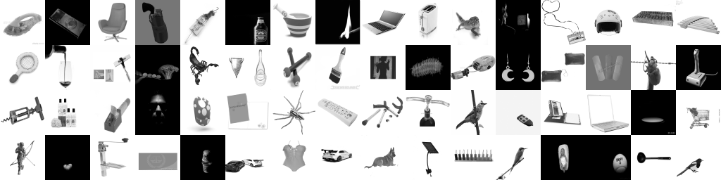
Figure 6: Highest probability images in ImageNet64 (test set).

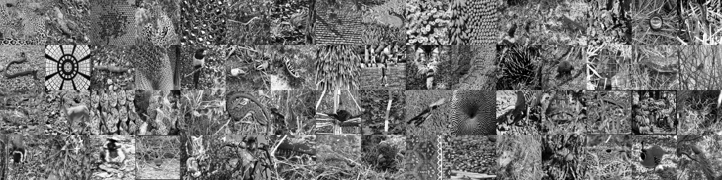
Figure 7: Lowest probability images in ImageNet64 (test set).

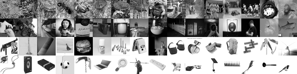
Figure 8: Images in ImageNet64 (test set) with linearly-spaced log probabilities.

References

- Bartosh et al. [2024] Grigory Bartosh, Dmitry P Vetrov, and Christian Andersson Naesseth. Neural flow diffusion models: Learnable forward process for improved diffusion modelling. Advances in Neural Information Processing Systems, 37:73952–73985, 2024.
- Bengio et al. [2013] Yoshua Bengio, Aaron Courville, and Pascal Vincent. Representation learning: A review and new perspectives. IEEE transactions on pattern analysis and machine intelligence, 35(8):1798–1828, 2013.
- Bhattacharya et al. [2025] Sagnik Bhattacharya, Abhiram R Gorle, Ahmed Mohsin, Ahsan Bilal, Connor Ding, Amit Kumar Singh Yadav, and Tsachy Weissman. ItDPDM: Information-theoretic discrete poisson diffusion model. arXiv preprint arXiv:2505.05082, 2025.
- Biroli et al. [2024] Giulio Biroli, Tony Bonnaire, Valentin De Bortoli, and Marc Mézard. Dynamical regimes of diffusion models. Nature Communications, 15(1):9957, 2024.
- Bruna and Han [2024] Joan Bruna and Jiequn Han. Provable posterior sampling with denoising oracles via tilted transport. Advances in Neural Information Processing Systems, 37:82863–82894, 2024.
- Chao et al. [2023] Chen-Hao Chao, Wei-Fang Sun, Bo-Wun Cheng, and Chun-Yi Lee. On investigating the conservative property of score-based generative models. International Conference on Machine Learning, 2023.
- Choi et al. [2022] Kristy Choi, Chenlin Meng, Yang Song, and Stefano Ermon. Density ratio estimation via infinitesimal classification. In International Conference on Artificial Intelligence and Statistics, pages 2552–2573. PMLR, 2022.
- Chrabaszcz et al. [2017] Patryk Chrabaszcz, Ilya Loshchilov, and Frank Hutter. A downsampled variant of imagenet as an alternative to the CIFAR datasets. arXiv preprint arXiv:1707.08819, 2017.
- Cohen et al. [2021] R Cohen, Y Blau, D Freedman, and E Rivlin. It has potential: Gradient-driven denoisers for convergent solutions to inverse problems. Adv Neural Information Processing Systems (NeurIPS), 34, 2021.
- Dinh et al. [2014] Laurent Dinh, David Krueger, and Yoshua Bengio. NICE: Non-linear independent components estimation. arXiv preprint arXiv:1410.8516, 2014.
- Dinh et al. [2017] Laurent Dinh, Jascha Sohl-Dickstein, and Samy Bengio. Density estimation using Real NVP. In International Conference on Learning Representations, 2017.
- Du et al. [2023] Yilun Du, Conor Durkan, Robin Strudel, Joshua B Tenenbaum, Sander Dieleman, Rob Fergus, Jascha Sohl-Dickstein, Arnaud Doucet, and Will Sussman Grathwohl. Reduce, reuse, recycle: Compositional generation with energy-based diffusion models and mcmc. In International conference on machine learning, pages 8489–8510. PMLR, 2023.
- Evans [1993] Lawrence C Evans. Partial differential equations, volume 19. American Mathematical Society, 1993.
- Guo et al. [2013] Dongning Guo, Shlomo Shamai, Sergio Verdú, et al. The interplay between information and estimation measures. Foundations and Trends® in Signal Processing, 6(4):243–429, 2013.
- Gutmann and Hyvärinen [2010] Michael Gutmann and Aapo Hyvärinen. Noise-contrastive estimation: A new estimation principle for unnormalized statistical models. In Proceedings of the thirteenth international conference on artificial intelligence and statistics, pages 297–304. JMLR Workshop and Conference Proceedings, 2010.
- Herbreteau et al. [2023] Sébastien Herbreteau, Emmanuel Moebel, and Charles Kervrann. Normalization-equivariant neural networks with application to image denoising. Advances in Neural Information Processing Systems, 36:5706–5728, 2023.
- Hinton [2002] Geoffrey E Hinton. Training products of experts by minimizing contrastive divergence. Neural computation, 14(8):1771–1800, 2002.
- Hinton et al. [1986] Geoffrey E Hinton, Terrence J Sejnowski, et al. Learning and relearning in Boltzmann machines. Parallel distributed processing: Explorations in the microstructure of cognition, 1(282-317):2, 1986.
- Ho et al. [2020] J Ho, A Jain, and P Abbeel. Denoising diffusion probabilistic models. Adv Neural Information Processing Systems (NeurIPS), 33, 2020.
- Ho et al. [2019] Jonathan Ho, Xi Chen, Aravind Srinivas, Yan Duan, and Pieter Abbeel. Flow++: Improving flow-based generative models with variational dequantization and architecture design. In International conference on machine learning, pages 2722–2730. PMLR, 2019.
- Horvat and Pfister [2024] Christian Horvat and Jean-Pascal Pfister. On gauge freedom, conservativity and intrinsic dimensionality estimation in diffusion models. In The Twelfth International Conference on Learning Representations, 2024.
- Hurault et al. [2021] Samuel Hurault, Arthur Leclaire, and Nicolas Papadakis. Gradient step denoiser for convergent plug-and-play. arXiv preprint arXiv:2110.03220, 2021.
- Hutchinson [1989] Michael F Hutchinson. A stochastic estimator of the trace of the influence matrix for laplacian smoothing splines. Communications in Statistics-Simulation and Computation, 18(3):1059–1076, 1989.
- Hyvärinen and Dayan [2005] Aapo Hyvärinen and Peter Dayan. Estimation of non-normalized statistical models by score matching. Journal of Machine Learning Research, 6(4), 2005.
- Kadkhodaie and Simoncelli [2020] Z Kadkhodaie and E P Simoncelli. Solving linear inverse problems using the prior implicit in a denoiser. arXiv preprint arXiv:2007.13640, Jul 2020.
- Kadkhodaie et al. [2024] Zahra Kadkhodaie, Florentin Guth, Eero P Simoncelli, and Stéphane Mallat. Generalization in diffusion models arises from geometry-adaptive harmonic representations. In The Twelfth International Conference on Learning Representations, 2024.
- Kamkari et al. [2024] Hamid Kamkari, Brendan Ross, Rasa Hosseinzadeh, Jesse Cresswell, and Gabriel Loaiza-Ganem. A geometric view of data complexity: Efficient local intrinsic dimension estimation with diffusion models. Advances in Neural Information Processing Systems, 37:38307–38354, 2024.
- Karczewski et al. [2025] Rafał Karczewski, Markus Heinonen, and Vikas Garg. Diffusion models as cartoonists! The curious case of high density regions. In The Thirteenth International Conference on Learning Representations, 2025.
- Kingma and Welling [2013] D P Kingma and M Welling. Auto-encoding variational bayes. arXiv preprint arXiv:1312.6114, 2013.
- Kingma et al. [2021] Diederik Kingma, Tim Salimans, Ben Poole, and Jonathan Ho. Variational diffusion models. Advances in neural information processing systems, 34:21696–21707, 2021.
- Kingma and Dhariwal [2018] Durk P Kingma and Prafulla Dhariwal. Glow: Generative flow with invertible 1x1 convolutions. Advances in neural information processing systems, 31, 2018.
- Koehler et al. [2023] Frederic Koehler, Alexander Heckett, and Andrej Risteski. Statistical efficiency of score matching: The view from isoperimetry. ICLR, 2023.
- Kong et al. [2023] Xianghao Kong, Rob Brekelmans, and Greg Ver Steeg. Information-theoretic diffusion. In The Eleventh International Conference on Learning Representations, 2023.
- Lai et al. [2023] Chieh-Hsin Lai, Yuhta Takida, Naoki Murata, Toshimitsu Uesaka, Yuki Mitsufuji, and Stefano Ermon. FP-diffusion: Improving score-based diffusion models by enforcing the underlying score fokker-planck equation. In International Conference on Machine Learning, pages 18365–18398. PMLR, 2023.
- LeCun and Huang [2005] Yann LeCun and Fu Jie Huang. Loss functions for discriminative training of energy-based models. In International workshop on artificial intelligence and statistics, pages 206–213. PMLR, 2005.
- LeCun et al. [2006] Yann LeCun, Sumit Chopra, Raia Hadsell, M Ranzato, Fujie Huang, et al. A tutorial on energy-based learning. Predicting structured data, 1(0), 2006.
- Lipman et al. [2023] Yaron Lipman, Ricky TQ Chen, Heli Ben-Hamu, Maximilian Nickel, and Matthew Le. Flow matching for generative modeling. In The Eleventh International Conference on Learning Representations, 2023.
- Miyasawa [1961] K Miyasawa. An empirical Bayes estimator of the mean of a normal population. Bull. Inst. Internat. Statist., 38:181–188, 1961.
- Mohan* et al. [2020] S Mohan*, Z Kadkhodaie*, E P Simoncelli, and C Fernandez-Granda. Robust and interpretable blind image denoising via bias-free convolutional neural networks. In Int’l Conf on Learning Representations (ICLR), Addis Ababa, Ethiopia, Apr 2020.
- Nichol and Dhariwal [2021] Alexander Quinn Nichol and Prafulla Dhariwal. Improved denoising diffusion probabilistic models. In International conference on machine learning, pages 8162–8171. PMLR, 2021.
- Raphan and Simoncelli [2011] M Raphan and E P Simoncelli. Least squares estimation without priors or supervision. Neural Computation, 23(2):374–420, Feb 2011. doi: 10.1162/NECO_a_00076.
- Raya and Ambrogioni [2023] Gabriel Raya and Luca Ambrogioni. Spontaneous symmetry breaking in generative diffusion models. Advances in Neural Information Processing Systems, 36:66377–66389, 2023.
- Reehorst and Schniter [2018] Edward T Reehorst and Philip Schniter. Regularization by denoising: Clarifications and new interpretations. IEEE transactions on computational imaging, 5(1):52–67, 2018.
- Rezende and Mohamed [2015] D Rezende and S Mohamed. Variational inference with normalizing flows. In Int’l Conf on Machine Learning (ICML), pages 1530–1538. PMLR, 2015.
- Robbins [1956] H Robbins. An empirical bayes approach to statistics. In Proc Third Berkeley Symposium on Mathematical Statistics and Probability, volume I, pages 157–163. University of CA Press, 1956.
- Romano et al. [2017] Yaniv Romano, Michael Elad, and Peyman Milanfar. The little engine that could: Regularization by denoising (red). SIAM Journal on Imaging Sciences, 10(4):1804–1844, 2017.
- Russakovsky et al. [2015] Olga Russakovsky, Jia Deng, Hao Su, Jonathan Krause, Sanjeev Satheesh, Sean Ma, Zhiheng Huang, Andrej Karpathy, Aditya Khosla, Michael Bernstein, et al. Imagenet large scale visual recognition challenge. International journal of computer vision, 115:211–252, 2015.
- Salimans and Ho [2021] Tim Salimans and Jonathan Ho. Should EBMs model the energy or the score? In Energy Based Models Workshop-ICLR 2021, 2021.
- Skreta et al. [2024] Marta Skreta, Lazar Atanackovic, Joey Bose, Alexander Tong, and Kirill Neklyudov. The superposition of diffusion models using the Itô density estimator. In The Thirteenth International Conference on Learning Representations, 2024.
- Sohl-Dickstein et al. [2015] J Sohl-Dickstein, E Weiss, N Maheswaranathan, and S Ganguli. Deep unsupervised learning using nonequilibrium thermodynamics. In Francis Bach and David Blei, editors, Proc 32nd Int’l Conf on Machine Learning (ICML), volume 37 of Proceedings of Machine Learning Research, pages 2256–2265, Lille, France, 07–09 Jul 2015. PMLR.
- Song and Ermon [2019] Y Song and S Ermon. Generative modeling by estimating gradients of the data distribution. Adv Neural Information Processing Systems (NeurIPS), 32, 2019.
- Song et al. [2021a] Y Song, J Sohl-Dickstein, D P Kingma, A Kumar, S Ermon, and B Poole. Score-based generative modeling through stochastic differential equations. In Int’l Conf on Learning Representations (ICLR), 2021a.
- Song and Kingma [2021] Yang Song and Diederik P Kingma. How to train your energy-based models. arXiv preprint arXiv:2101.03288, 2021.
- Song et al. [2021b] Yang Song, Conor Durkan, Iain Murray, and Stefano Ermon. Maximum likelihood training of score-based diffusion models. Advances in Neural Information Processing Systems, 34:1415–1428, 2021b.
- Stanczuk et al. [2022] Jan Stanczuk, Georgios Batzolis, Teo Deveney, and Carola-Bibiane Schönlieb. Your diffusion model secretly knows the dimension of the data manifold. arXiv preprint arXiv:2212.12611, 2022.
- Tempczyk et al. [2022] Piotr Tempczyk, Rafał Michaluk, Lukasz Garncarek, Przemysław Spurek, Jacek Tabor, and Adam Golinski. LIDL: Local intrinsic dimension estimation using approximate likelihood. In International Conference on Machine Learning, pages 21205–21231. PMLR, 2022.
- Tenenbaum et al. [2000] Joshua B Tenenbaum, Vin de Silva, and John C Langford. A global geometric framework for nonlinear dimensionality reduction. science, 290(5500):2319–2323, 2000.
- Theis et al. [2016] L Theis, A van den Oord, and M Bethge. A note on the evaluation of generative models. In International Conference on Learning Representations (ICLR 2016), pages 1–10, 2016.
- Thiry and Guth [2024] Louis Thiry and Florentin Guth. Classification-denoising networks. arXiv preprint arXiv:2410.03505, 2024.
- Ulyanov et al. [2016] Dmitry Ulyanov, Andrea Vedaldi, and Victor Lempitsky. Instance normalization: The missing ingredient for fast stylization. arXiv preprint arXiv:1607.08022, 2016.
- Van den Oord et al. [2016] Aaron Van den Oord, Nal Kalchbrenner, Lasse Espeholt, Oriol Vinyals, Alex Graves, et al. Conditional image generation with PixelCNN decoders. Advances in neural information processing systems, 29, 2016.
- Vershynin [2018] Roman Vershynin. High-dimensional probability: An introduction with applications in data science, volume 47. Cambridge university press, 2018.
- Vincent [2011] P Vincent. A connection between score matching and denoising autoencoders. Neural Computation, 23(7):1661–1674, 2011.
- Wainwright [2019] Martin J Wainwright. High-dimensional statistics: A non-asymptotic viewpoint, volume 48. Cambridge university press, 2019.
- Wu and Verdú [2011] Yihong Wu and Sergio Verdú. MMSE dimension. IEEE Transactions on Information Theory, 57(8):4857–4879, 2011.
- Yadin et al. [2024] Shahar Yadin, Noam Elata, and Tomer Michaeli. Classification diffusion models. arXiv preprint arXiv:2402.10095, 2024.
- Yedidia et al. [2005] Jonathan S Yedidia, William T Freeman, and Yair Weiss. Constructing free-energy approximations and generalized belief propagation algorithms. IEEE Transactions on information theory, 51(7):2282–2312, 2005.
- Zhai et al. [2024] Shuangfei Zhai, Ruixiang Zhang, Preetum Nakkiran, David Berthelot, Jiatao Gu, Huangjie Zheng, Tianrong Chen, Miguel Angel Bautista, Navdeep Jaitly, and Josh Susskind. Normalizing flows are capable generative models. arXiv preprint arXiv:2412.06329, 2024.
- Zheng et al. [2023] Kaiwen Zheng, Cheng Lu, Jianfei Chen, and Jun Zhu. Improved techniques for maximum likelihood estimation for diffusion ODEs. In International Conference on Machine Learning, pages 42363–42389. PMLR, 2023.