Drawdowns, Drawups, and Occupation Times under General Markov Models

Abstract

Drawdown risk, an important metric in financial risk management, poses significant computational challenges due to its highly path-dependent nature. This paper proposes a unified framework for computing five important drawdown quantities introduced in Landriault et al. (2015) and Zhang (2015) under general Markov models. We first establish linear systems and develop efficient algorithms for such problems under continuous-time Markov chains (CTMCs), and then establish their theoretical convergence to target quantities under general Markov models. Notably, the proposed algorithms for most quantities achieve the same complexity order as those for path-independent problems: cubic in the number of CTMC states for general Markov models and linear when applied to diffusion models. Rigorous convergence analysis is conducted under weak regularity conditions, and extensive numerical experiments validate the accuracy and efficiency of the proposed algorithms.

Keywords: Continuous-time Markov chain approximation; Drawdowns; Drawups; Occupation times; Markov models

MSC: 60J28; 60J60; 60J76; 91G20; 91G30; 91G60

1 Introduction

Drawdown, defined as the magnitude of decline of the asset price from its historical peak, has emerged as a widely adopted downside risk metric in financial markets. Its prominence is evidenced by growing scholarly and industrial interest, particularly in applications such as performance evaluation of investment funds and algorithmic trading strategies, where maximum drawdown is routinely reported as a key robustness indicator. Notably, empirical studies increasingly associate irrational trading behaviors, including panic selling and momentum overreaction, with exposure to extreme drawdown events.

Various drawdown quantities have been systematically examined in the academic literature, including the first passage time of drawdown processes (Taylor, 1975; Lehoczky, 1977; Douady et al., 2000; Magdon-Ismail et al., 2004; Hadjiliadis and Večeř, 2006; Pospisil et al., 2009; Zhang and Hadjiliadis, 2010; Mijatović and Pistorius, 2012; Zhang, 2015; Landriault et al., 2017b; Zhang and Li, 2023c), maximum drawdown (Magdon-Ismail and Atiya, 2004; Pospisil and Vecer, 2008, 2010; Schuhmacher and Eling, 2011), speed and duration of drawdown (Zhang and Hadjiliadis, 2012; Landriault et al., 2017a; Cui and Nguyen, 2018; Li et al., 2024), along with drawdown-linked insurance products and derivatives (Shepp and Shiryaev, 1993; Asmussen et al., 2004; Avram et al., 2004; Vecer, 2006, 2007; Zhang et al., 2013; Landriault et al., 2015; Cui and Nguyen, 2016; Zhang et al., 2021). Furthermore, drawdown constraints have been rigorously embedded within stochastic control frameworks for portfolio optimization (Grossman and Zhou, 1993; Cvitanic and Karatzas, 1995; Chekhlov et al., 2005; Cherny and Obłój, 2013), marking a paradigm shift in risk-aware asset allocation methodologies.

Among the extensive literature on drawdown and related derivatives, seminal works by Landriault et al. (2015) and Zhang (2015) made significant strides in quantifying the frequency of drawdowns, drawdowns preceding drawups (vice versa), and occupation times of drawdown processes. These drawdown quantities are especially useful in financial engineering applications and of theoretical importance in stochastic modeling. However, these foundational studies predominantly assume a diffusion process or even a Brownian motion, as the underlying model, fail to capture the empirical reality of financial markets where discontinuous price movements (jumps) frequently occur. To address this limitation and enable robust evaluation of these drawdown quantities under general Markov models, we develop a novel computational framework based on the continuous-time Markov chain (CTMC) approximation.

For a stochastic process $\{X_{t}\}_{t\geq 0}$, the drawdown process $\{D_{t}\}_{t\geq 0}$ and drawup process $\{\widehat{D}_{t}\}_{t\geq 0}$ can be formally defined as

$$D_{t}=\sup_{0\leq s\leq t}X_{s}-X_{t}~~\text{and}~~\widehat{D}_{t}=X_{t}-\inf_{0\leq s\leq t}X_{s},\qquad t\geq 0,$$

respectively. The drawdown time is then defined as the first passage time of the drawdown process $D$ reaches a predefined threshold level $a$, i.e., $\tau^{X}_{a}=\inf\{t\geq 0:D_{t}\geq a\}$ and similarly the drawup time is $\widehat{\tau}^{X}_{b}=\inf\{t\geq 0:\widehat{D}_{t}\geq b\}$. Inspired by Landriault et al. (2015) and Zhang (2015), we focus on the following five drawdown quantities under general Markov models: (1) The drawdown time proceeding the drawup time; (2) The generalized occupation time of the Markov process until the drawdown time; (3) The generalized occupation time of the drawdown process until the drawdown time; (4) The $n$-th drawdown time without recovery; (5) The $n$-th drawdown time with recovery. More specifically, we first approximate the Markov process $X$ by a CTMC and then price the target quantities under the CTMC. The CTMC approximation method has been extensively used for derivative pricing under Markov models. Notable applications include European and barrier options (Mijatović and Pistorius, 2013), American options (Eriksson and Pistorius, 2015), Asian options (Song et al., 2013; Cai et al., 2015; Cui et al., 2018), occupation time derivatives (Zhang and Li, 2022), lookback options (Zhang and Li, 2023a), Parisian options (Zhang and Li, 2023b), autocallable products (Cui et al., 2024), and drawdown derivatives (Zhang et al., 2021; Zhang and Li, 2023c; Li et al., 2024). Working under the CTMC model, we can establish rigorous characterizations of these five target quantities through dedicated linear system formulations and develop efficient recursive procedures to reduce the complexity of solving these linear systems. For most drawdown quantities, our methodology achieves computational complexity scaling as $\mathcal{O}(N^{3})$ with $N$ CTMC states under general Markov models, while attaining complexity $\mathcal{O}(N)$ when applied to diffusion models, thereby achieving computational parity with path-independent valuations (e.g., European option pricing) under equivalent model configurations. Finally, we perform rigorous convergence analysis under weak regularity conditions, and conduct extensive numerical experiments to demonstrate the accuracy and efficiency of the proposed algorithms.

Our contributions to the literature are three-fold:

• We have proposed efficient algorithms for evaluating five important drawdown quantities under general Markov models, overcoming the restrictive Lévy process/diffusion process/Brownian motion assumptions prevalent in existing literature (e.g., Mijatović and Pistorius (2012), Landriault et al. (2015), and Zhang (2015)). In addition, the CTMC approximation has been applied to the analysis of drawdown risk (Zhang and Li, 2023c), American drawdown option pricing (Zhang et al., 2021), and the speed and duration of drawdown (Li et al., 2024) under general Markov models, while we extend its application to various highly path-dependent drawdown quantities. Our results are nontrivial extensions of the existing papers. For example, we investigate occupation times of the underlying and drawdown/drawup process up to the drawdown/drawup time, which adds another layer of path-dependency.

• We have established the convergence analysis of the proposed algorithms. The analysis adopts the techniques used in Zhang and Li (2023c) but with important and nontrivial modifications to handle the additional path-dependency as mentioned above.

• We contribute to ample financial engineering applications of drawdown quantities. Specifically, we price various financial products, including digital options associated with the occupation times of the Markov/drawdown processes and insurance products associated with the frequency of relative drawdowns with/without recovery.

The remainder of the paper is structured as follows. In Section 2, we introduce preliminary results of drawdown analysis under the CTMC model. In Section 3, we derive linear systems for five drawdown quantities via the CTMC approximation and propose efficient algorithms for solving these systems. We perform convergence analysis of the proposed algorithms under some mild conditions in Section 4, and conduct numerical experiments to demonstrate the accuracy and efficiency of our algorithms in Section 5. Finally, we conclude the paper in Section 6. The construction of the CTMC approximation and proofs are provided in Appendices A and B, respectively.

2 Preliminaries

Consider a 1D time-homogeneous Markov process $X$ living on an interval $I\subseteq\mathbb{R}$ with its infinitesimal generator $\mathcal{L}$ acting on $g\in C^{2}_{c}(I)$ as follows:

$$\mathcal{L}g(x)=b(x)g^{\prime}(x)+\frac{1}{2}\sigma^{2}(x)g^{\prime\prime}(x)+\int_{\mathbb{R}}\big{(}g(x+y)-g(x)-yg^{\prime}(x)\mathbf{1}_{\{|y|\leq 1\}}\big{)}\,\nu(x,\mathop{}\!\mathrm{d}y),$$ (1)

where $b(x)$ is the drift, $\sigma(x)$ is the diffusion coefficient, and $\nu(x,\mathop{}\!\mathrm{d}y)$ is the state-dependent jump measure satisfying $\int_{|y|\leq 1}y^{2}\,\nu(x,\mathop{}\!\mathrm{d}y)<\infty$ for all $x\in I$. The class of models characterized by (1) is very general as it subsumes diffusions, jump-diffusions, and pure-jump models, and allows the jump intensity to be state-dependent with finite or infinite jump activity and finite or infinite jump variation.

The process $X$ can be approximated by a continuous-time Markov chain (CTMC) $Y$ with the finite state space $\mathbb{S}=\{y_{0},y_{1},\cdots,y_{N}\},$ where $y_{0}<y_{1}<\cdots<y_{N}$ and $y_{0}$ and $y_{N}$ are absorbing states. The details regarding the construction of the CTMC can be found in Appendix A. Denote by $\bm{G}$ the transition rate matrix of $Y$, whose elements satisfy that $G(x,y)\geq 0$ for $y\in\mathbb{S}\backslash\{x\}$ and $G(x,x)=-\sum_{y\in\mathbb{S}\backslash\{x\}}G(x,y)$ for all $x\in\mathbb{S}$. The infinitesimal generator of the CTMC $Y$ is then formulated as: for any function $g:\mathbb{S}\to\mathbb{R}$,

$$\mathcal{G}g(x)=\sum_{y\in\mathbb{S}}G(x,y)g(y),\qquad x\in\mathbb{S}.$$ (2)

In the following, for any $x$, define by $x^{+}=\min\{y\in\mathbb{S},~y>x\}$ the right grid point next to $x$.

2.1 The First Passage Time of the CTMC

For any $S\subseteq\mathbb{R}$, the first passage time of the CTMC $Y$ is defined as follows:

$$T_{S}:=\inf\{t>0:Y_{t}\notin S\}.$$ (3)

We consider the following quantity:

$$P_{S}(k,x;f):=\mathbb{E}\big{[}e^{-\int_{0}^{T_{S}}k(Y_{s})\mathop{}\!\mathrm{d}s}\mathbf{1}_{\{T_{S}<\infty\}}f(Y_{T_{S}})\,\big{|}\,Y_{0}=x\big{]},$$ (4)

where $k,f:\mathbb{S}\to\mathbb{R}$.

Lemma 1.

The quantity $P_{S}(k,x;f)$ satisfies the following linear system:

$$\begin{cases}(k(x)-\mathcal{G})P_{S}(k,x;f)=0,\qquad&x\in\mathbb{S}\cap S,\\ P_{S}(k,x;f)=f(x),\qquad&x\in\mathbb{S}\backslash S,\end{cases}$$ (5)

where $\mathcal{G}$ is the infinitesimal generator of the CTMC specified by (2).

The proof of Lemma 1 is analogous to that of Proposition 3.1 in Zhang and Li (2023c) and hence is omitted here. Following Zhang and Li (2023c), the linear system above admits a closed-form solution. More specifically, define ${\boldsymbol{P}}_{S}(k;f)=\big{(}P_{S}(k,x;f)\big{)}_{x\in\mathbb{S}},$ then

$${\boldsymbol{P}}_{S}(k;f)=({\boldsymbol{I}}_{S^{c}}+{\boldsymbol{I}}_{S}\operatorname{diag}({\boldsymbol{k}})-{\boldsymbol{I}}_{S}\,{\boldsymbol{G}})^{-1}{\boldsymbol{I}}_{S^{c}}{\boldsymbol{f}}.$$ (6)

Here, ${\boldsymbol{f}}=(f(x))_{x\in\mathbb{S}}$, ${\boldsymbol{k}}=(k(x))_{x\in\mathbb{S}}$, ${\boldsymbol{I}}_{S}=(\mathbf{1}_{\{z=x,\,x\in S\}})_{x,\,z\in\mathbb{S}}$, and ${\boldsymbol{I}}_{S^{c}}=(\mathbf{1}_{\{z=x,\,x\in S^{c}\}})_{x,\,z\in\mathbb{S}}$. It is noteworthy that the dependence of the solution on $f$ is linear.

Remark 1.

The Laplace transform of the first passage time $T_{S}$ can be obtained as a special case by setting $k(x)\equiv q$ and $f(x)\equiv 1$.

2.2 The First Passage Time of the Drawdown Process of the CTMC

Write $\overline{Y}_{t}=\sup_{0\leq u\leq t}Y_{u}$ and denote by $\tau_{a}=\mathrm{inf}\{t\geq 0:\overline{Y}_{t}-Y_{t}\geq a\}$ the first passage time of the drawdown process of the CTMC $Y$ to the level $a>0$. We call $\tau_{a}$ the drawdown time. Define

$$Q_{a}(q,x;f):=\mathbb{E}_{x}\big{[}e^{-q\tau_{a}}\mathbf{1}_{\{\tau_{a}<\infty\}}f(Y_{\tau_{a}})\big{]},$$ (7)

where $q\in\mathbb{C}$ with $\Re(q)>0$, $f:\mathbb{S}\to\mathbb{R}$, and $\mathbb{E}_{x}[\cdot]=\mathbb{E}[\cdot\,|\,Y_{0}=x,\,\overline{Y}_{0}=x]$.

Lemma 2.

For any $q\in\mathbb{C}$ with $\Re(q)>0$ and $x\in\mathbb{S}$, the quantity $Q_{a}(q,x;f)$ satisfies the following linear system:

$$Q_{a}(q,x;f)=P_{(x-a,x]}(q,x;f(\cdot)\mathbf{1}_{\{\cdot\leq x-a\}})+\sum_{y\in\mathbb{S},\,y>x}P_{(x-a,x]}\big{(}q,x;\mathbf{1}_{\{\cdot=y\}}\big{)}Q_{a}(q,y;f).$$ (8)

The proof of Lemma 2 is very similar to that of Theorem 3.1 in Zhang and Li (2023c) and hence is omitted here. The computationally efficient recursive algorithm proposed by Zhang and Li (2023c) can be employed for solving the linear system (8). The key steps of their approach can be summarized as follows:

• Step 1: $Q_{a}(q,y_{N};f)=0$ as $y_{N}$ is an absorbing state.

• Step 2: Assume $x=y_{\eta_{x}}$ for some integer $\eta_{x}$. Calculate $Q_{a}(q,y_{i};f)$ by running the backward from $i={N-1}$ to $i=\eta_{x}$:

  • Compute the quantities $P_{(y_{i}-a,y_{i}]}(q,y_{i};f(\cdot)\mathbf{1}_{\{\cdot\leq y_{i}-a\}})$ and $P_{(y_{i}-a,y_{i}]}\big{(}q,y_{i};\mathbf{1}_{\{\cdot=y_{j}\}}\big{)}$ for all $j>i$ via (6);

  • Compute $Q_{a}(q,y_{i};f)$ via (8).

Significant reduction of the computational cost can be achieved in the following two cases.

Case 1: the Markov process $X$ is a Lévy process. A CTMC $Y$ with the state space $\mathbb{S}=h\mathbb{Z}$ is chosen to approximate $X$ so that $Y$ itself is also a Lévy process. Here, $h>0$ and $\mathbb{Z}$ denotes the set of integers. In this case, $P_{S}(q,x;f)=P_{S-x}(q,0;f(x+\cdot))$ and (8) can be rewritten as follows:

$$Q_{a}(q,x;f) =\sum_{y\in\mathbb{S},\,y\leq x-a}P_{(x-a,x]}\big{(}q,x;\mathbf{1}_{\{\cdot=y\}}\big{)}f(y)+\sum_{y\in\mathbb{S},\,y>x}P_{(x-a,x]}\big{(}q,x;\mathbf{1}_{\{\cdot=y\}}\big{)}Q_{a}(q,y;f)$$

$$=\sum_{y\in\mathbb{S},\,y\leq-a}P_{(-a,0]}\big{(}q,0;\mathbf{1}_{\{\cdot=y\}}\big{)}f(y+x)+\sum_{y\in\mathbb{S},\,y>0}P_{(-a,0]}\big{(}q,0;\mathbf{1}_{\{\cdot=y\}}\big{)}Q_{a}(q,y+x;f).$$

Obviously, it suffices to compute $P_{(-a,0]}\big{(}q,0;\mathbf{1}_{\{\cdot=y_{i}\}}\big{)}$ for $y_{i}\leq-a$ and $y_{i}>0$ via (6) to obtain $Q_{a}(q,x;f)$ recursively.

Case 2: the Markov process $X$ is a diffusion process. The resulting CTMC is a birth-death process and (8) can be simplified as follows:

$$Q_{a}(q,x;f) =P_{(x-a,x]}(q,x;\mathbf{1}_{\{\cdot=(x-a)^{\ominus}\}})f((x-a)^{\ominus})+P_{(x-a,x]}(q,x;\mathbf{1}_{\{\cdot=x^{+}\}})Q_{a}(q,x^{+};f),$$ (9)

where $(x-a)^{\ominus}=\sup\{y\in\mathbb{S}:y\leq x-a\}$. In this case, $P_{(x-a,x]}(q,x;\mathbf{1}_{\{\cdot=(x-a)^{\ominus}\}})$ and $P_{(x-a,x]}(q,x;\mathbf{1}_{\{\cdot=x^{+}\}})$ can be constructed from two independent solutions $\psi^{\pm}$ as follows: (see Zhang and Li (2023c))

$$P_{(x-a,x]}(q,x;\mathbf{1}_{\{\cdot=x^{+}\}})=\frac{\psi^{+}(q,x)\psi^{-}(q,(x-a)^{\ominus})-\psi^{+}(q,(x-a)^{\ominus})\psi^{-}(q,x)}{\psi^{+}(q,x^{+})\psi^{-}(q,(x-a)^{\ominus})-\psi^{+}(q,(x-a)^{\ominus})\psi^{-}(q,x^{+})},$$ (10)

$$P_{(x-a,x]}(q,x;\mathbf{1}_{\{\cdot=(x-a)^{\ominus}\}})=\frac{\psi^{+}(q,x^{+})\psi^{-}(q,x)-\psi^{+}(q,x)\psi^{-}(q,x^{+})}{\psi^{+}(q,x^{+})\psi^{-}(q,(x-a)^{\ominus})-\psi^{+}(q,(x-a)^{\ominus})\psi^{-}(q,x^{+})}.$$ (11)

Here, $\psi^{\pm}$ satisfy the following linear systems:

$$(q-\mathcal{G})\psi^{\pm}(q,x)=0,\qquad x\in\mathbb{S}\backslash\{y_{0},y_{N}\},$$ (12)

with boundary conditions: $\psi^{+}(q,y_{0})=\psi^{-}(q,y_{N})=0$ and $\psi^{-}(q,y_{0})=\psi^{+}(q,y_{N})=1$.

3 Drawdowns, Drawups, and Occupation Times

In this section, we derive linear systems for five drawdown quantities under the CTMC and then propose efficient algorithms for solving these linear systems.

3.1 The Drawdown Time Preceding the Drawup Time

Write $\underline{Y}_{t}=\inf_{0\leq u\leq t}Y_{u}$ and denote by $\widehat{\tau}_{b}=\mathrm{inf}\{t\geq 0:Y_{t}-\underline{Y}_{t}\geq b\}$ the first passage time of the drawup process of the CTMC $Y$ to the level $b>0$. $\widehat{\tau}_{b}$ is called the drawup time. We consider the drawdown time $\tau_{a}$ and the drawup time $\widehat{\tau}_{b}$, especially when the former precedes the latter, and define the following quantity:

$$A(q,x,y):=\mathbb{E}_{x,y}\big{[}e^{-q\tau_{a}}\mathbf{1}_{\{\tau_{a}<\widehat{\tau}_{b}\}}f(Y_{\tau_{a}})\big{]}.$$ (13)

Here, $q\in\mathbb{C}$ with $\Re(q)>0$, $f:\mathbb{S}\to\mathbb{R}$, and $\mathbb{E}_{x,y}[\cdot]=\mathbb{E}[\cdot\,|\,Y_{0}=x,\,\overline{Y}_{0}=x,\,\underline{Y}_{0}=y]$.

Proposition 1.

Suppose $b\geq a$. For any $q\in\mathbb{C}$ with $\Re(q)>0$, $x\in\mathbb{S}$, and $y\in\mathbb{S}\cap(x-a,x]$, the quantity $A(q,x,y)$ satisfies the following linear system:

$$A(q,x,y)= ~P_{(x-a,x]}(q,x;f(\cdot)\mathbf{1}_{\{\cdot\leq x-a\}})$$ (14)

$$~+\sum_{z\in\mathbb{S}\cap(x,y+b),\,w\in\mathbb{S}\cap((x-a)\vee(z-b),y]}R_{(x-a,x]}(q,x,y;\mathbf{1}_{\{\cdot=z,\,\tilde{\cdot}=w\}})A(q,z,w),$$

where

$$R_{(\ell,r]}(q,x,y;g):=\mathbb{E}\big{[}e^{-qT_{r}^{+}}\mathbf{1}_{\{T_{\ell}^{-}>T_{r}^{+}\}}g(Y_{T_{r}^{+}},\underline{Y}_{T_{r}^{+}})\,\big{|}\,Y_{0}=x,\,\underline{Y}_{0}=y\big{]},$$ (15)

which satisfies the following linear system: for $x,y\in\mathbb{S}$ with $x\geq y$,

$$\begin{cases}qR_{(\ell,r]}(q,x,y;g)-\sum\limits_{z\in\mathbb{S}}G(x,z)R_{(\ell,r]}(q,z,y\wedge z;g)=0,\qquad&x\in(\ell,r],\\ R_{(\ell,r]}(q,x,y;g)=g(x,y)\mathbf{1}_{\{x>r\}},\qquad&x\notin(\ell,r].\end{cases}$$ (16)

Here, $\ell<r$, $T_{r}^{+}:=T_{(-\infty,r]}$, and $T_{\ell}^{-}:=T_{(\ell,\infty)}$.

Proof.

The proof of Proposition 1 is given in Appendix B.1. ∎

Next, we develop an efficient algorithm to solve the linear systems (14) and (16) recursively; see Algorithm 1.

Algorithm 1 Calculate $A(q,x,y)$

Assumptions $\eta_{x}:=\{i:y_{i}=x\}$ and $\eta_{y}:=\{i:y_{i}=y\}$.

Notations $i_{a}:=\min\{j:y_{j}>y_{i}-a\},~i_{b}:=\min\{j:y_{j}>y_{i}-b\}$, $\bm{G}:=\{G(y_{m},y_{l})\}_{m,{l}=0}^{N}$, $\bm{I}_{m}$ denotes an ${m\times m}$ identity matrix, and $\text{Diag}(\bm{c})$ denotes the diagonal matrix with diagonal elements being $\bm{c}$.

Input $\mathbb{S},~\bm{G},~f,~\eta_{x},~\eta_{y},$ and $q$.

Initialize $A(q,y_{N},\cdot)\leftarrow 0$

for $i=N-1$ to $\eta_{x}$ do

  $\bm{G}_{i}\leftarrow\{G(y_{m},y_{l})\}_{m,{l}=i_{a}}^{i}$,    $\bm{e}_{i}\leftarrow\text{Diag}(\{\mathbf{1}_{\{y_{m}=y_{i}\}}\}_{m=i_{a}}^{i})$,

  $\bm{G}_{i}^{-}\leftarrow\{\{G(y_{m},y_{l})\}_{m=i_{a}}^{i}\}_{{l}=0}^{i_{a}-1}$,    $\bm{G}_{i}^{+}\leftarrow\{\{G(y_{m},y_{l})\}_{m=i_{a}}^{i}\}_{l=i+1}^{N}$,

  $\bm{A}_{i}^{+}\leftarrow\{\{A(q,y_{m},y_{l})\}_{m=i+1}^{N}\}_{{l}=i_{b}}^{i_{a}}$,    $\bm{f}_{i}\leftarrow\{f(y_{m})\}_{m=0}^{i_{a}-1}$,

  $\{g_{i,n}(\cdot,\tilde{\cdot})\}_{n=i_{a}}^{i-1}\leftarrow\bigg{\{}\sum\limits_{y_{i}<y_{m}<y_{n}+b,\,y_{i_{a}}\vee y_{m_{b}}<y_{l}\leq y_{n}}\mathbf{1}_{\{\cdot=y_{m},\,\tilde{\cdot}=y_{l}\}}A(q,y_{m},y_{l})\bigg{\}}_{n=i_{a}}^{i}$,

  $P_{(y_{i}-a,y_{i}]}(q,y_{i};f)\leftarrow-\bm{e}_{i}(\bm{G}_{i}-q\bm{I}_{i-i_{a}+1})^{-1}(\bm{G}_{i}^{-}\bm{f}_{i})$,

  $\{A(q,y_{i},y_{l})\}_{{l}=i_{b}}^{i_{a}}\leftarrow P_{(y_{i}-a,y_{i}]}(q,y_{i};f)-\bm{e}_{i}(\bm{G}_{i}-q\bm{I}_{i-i_{a}+1})^{-1}(\bm{G}_{i}^{+}\bm{A}_{i}^{+})$,

  for $j=i_{a}+1$ to $i$ do

   $\bm{G}_{i,j}\leftarrow\{G(y_{m},y_{l})\}_{m,{l}=j}^{i}$,    $\bm{e}_{i,j}=\text{Diag}(\{\mathbf{1}_{\{y_{m}=y_{i}\}}\}_{m=j}^{i})$,

   $\bm{G}_{i,j}^{-}\leftarrow\{\{G(y_{m},y_{l})\}_{m=j}^{i}\}_{{l}=i_{a}}^{j-1}$,    $\bm{G}_{i,j}^{+}\leftarrow\{\{G(y_{m},y_{l})\}_{m=j}^{i}\}_{{l}=i+1}^{N}$,

   $\bm{R}_{i,j}^{-}\leftarrow\{R_{(y_{i}-a,y_{i}]}(q,y_{m},y_{m};g_{i,m})\}_{m=i_{a}}^{j-1}$,    $\bm{A}_{i,j}^{+}\leftarrow\{A(q,y_{m},y_{j})\}_{m=i+1}^{N}$,

   $A(q,y_{i},y_{j})\leftarrow P_{(y_{i}-a,y_{i}]}(q,y_{i};f)-\bm{e}_{i,j}(\bm{G}_{i,j}-q\bm{I}_{i-j+1})^{-1}(\bm{G}_{i,j}^{-}\bm{R}_{i,j}^{-}+\bm{G}_{i,j}^{+}\bm{A}_{i,j}^{+})$.

  end for

end for

return $A(q,y_{\eta_{x}},y_{\eta_{y}})$

Remark 2.

The complexity of Algorithm 1 is dominated by the calculations of inverse matrices and matrix multiplications. For each fixed $i$, when $j$ ranges from $i_{a}+1$ to $i$, the matrix $\bm{G}_{i,j}-q\bm{I}_{i-j+1}$ in each recursion step can be expressed as the matrix in the previous step plus a sum of rank-one matrices. This observation enables us to utilize the Sherman–Morrison–Woodbury formula (Woodbury, 1950) to efficiently compute $(\bm{G}_{i,j}-q\bm{I}_{i-j+1})^{-1}$ from the inverse matrix in the previous recursion step, see Zhang and Li (2023c, Section 3.1) for more details. Consequently, the complexity of calculating inverse matrices in the inner loop is $\mathcal{O}(N^{3})$. Furthermore, when $i$ decreases from $N-1$ to $\eta_{x}$, the Sherman–Morrison–Woodbury formula can be applied again, resulting in a complexity of order $\mathcal{O}(N^{4})$ for the whole loops. Consequently, the overall complexity of computing inverse matrices is $\mathcal{O}(N^{4})$.

The complexity in the calculations of matrix multiplications is of order $\mathcal{O}(N^{3})$ instead of $\mathcal{O}(N^{4})$. Take matrix multiplications $\bm{G}_{i,j}^{-}\bm{R}_{i,j}^{-}$ with $i=N-1,\dots,\eta_{x}$ and $j=i_{a}+1,\dots,i$ for example. The computational cost can be reduced as follows. Introduce two new matrices $\widetilde{\bm{G}}_{i,j+1}^{-}$ and $\widetilde{\bm{G}}_{i,j}^{-}$ by expanding $\bm{G}_{i,j+1}^{-}$ and $\bm{G}_{i,j}^{-}$ as follows:

$$\widetilde{\bm{G}}_{i,j+1}^{-}:=\begin{bmatrix}\bm{G}_{i,j+1}^{-}\\ \bm{0}_{1\times(j-i_{a}+1)}\end{bmatrix},\quad\quad\quad\widetilde{\bm{G}}_{i,j}^{-}:=\begin{bmatrix}\bm{G}_{i,j}^{-}&\bm{0}_{(i-j+1)\times 1}\end{bmatrix},$$ (17)

where $\bm{0}_{m\times n}$ is an $m\times n$ zero matrix. By construction, $\widetilde{\bm{G}}_{i,j+1}^{-}-\widetilde{\bm{G}}_{i,j}^{-}$ is a sparse matrix as only the last row and column contain non-zero elements. The sparsity ensures that the calculation of the matrix multiplication $(\widetilde{\bm{G}}_{i,j+1}^{-}-\widetilde{\bm{G}}_{i,j}^{-})\bm{R}_{i,j+1}^{-}$ only requires $\mathcal{O}(N)$ operations. Moreover, notice that

$$\widetilde{\bm{G}}_{i,j+1}^{-}\bm{R}_{i,j+1}^{-}= (\widetilde{\bm{G}}_{i,j+1}^{-}-\widetilde{\bm{G}}_{i,j}^{-})\bm{R}_{i,j+1}^{-}+\widetilde{\bm{G}}_{i,j}^{-}\bm{R}_{i,j+1}^{-}$$ (18)

$$= (\widetilde{\bm{G}}_{i,j+1}^{-}-\widetilde{\bm{G}}_{i,j}^{-})\bm{R}_{i,j+1}^{-}+\bm{G}_{i,j}^{-}\bm{R}_{i,j}^{-}.$$

As a result, once $\bm{G}_{i,j}^{-}\bm{R}_{i,j}^{-}$ has been calculated, the complexity of evaluating $\widetilde{\bm{G}}_{i,j+1}^{-}\bm{R}_{i,j+1}^{-}$ is $\mathcal{O}(N)$. So is $\bm{G}_{i,j+1}^{-}\bm{R}_{i,j+1}^{-}$. When $j$ increases from $i_{a}+1$ to $i$ and $i$ decreases from $N-1$ to $\eta_{x}$, the computations of these matrix multiplications are of $\mathcal{O}(N^{3})$ complexity.

Therefore, the overall complexity of Algorithm 1 is $\mathcal{O}(N^{4})$. In particular, when the Markov process $X$ is a diffusion process, the overall complexity of Algorithm 1 can be reduced to $\mathcal{O}(N^{2})$. In this case, similar to (10), the quantity $A(q,y_{i},y_{j})$ can be represented in terms of the vector $\{\psi^{\pm}(q,y_{m})\}_{m=0}^{N}$, which requires $\mathcal{O}(N)$ operations by solving the linear systems (12). Thus, one circumvents the computations of inverse matrices and matrix multiplications, as previously discussed. When $i$ decreases from $N-1$ to $\eta_{x}$ and $j$ ranges from $i_{a}+1$ to $i$, the overall complexity is $\mathcal{O}((N-\eta_{x})(i-i_{a}))+O(N)$, which simplifies to $O(N^{2})$.

Remark 3.

For any $q\in\mathbb{C}$ with $\Re(q)>0$, $x\in\mathbb{S}$, and $y\in(x-b,x-a]$, the quantity $A(q,x,y)$ satisfies the following simpler linear system:

$$A(q,x,y)=P_{(x-a,x]}(q,x;f(\cdot)\mathbf{1}_{\{\cdot\leq x-a\}})+\sum_{z\in\mathbb{S}\cap(x,y+b)}P_{(x-a,x]}(q,x;\mathbf{1}_{\{\cdot=z\}})A(q,z,y),$$ (19)

which can be solved in analogous to the quantity $Q_{a}(q,x;f)$.

Remark 4.

The case $b<a$ is more complicated and we leave it for future work.

3.2 The Generalized Occupation Time of the CTMC until the Drawdown Time

Next, we consider the generalized occupation time of the CTMC $Y$ until the drawdown time $\tau_{a}$ and introduce the following quantity:

$$B(k,x)=\mathbb{E}_{x}\big{[}e^{-\int_{0}^{\tau_{a}}k(Y_{s})\mathop{}\!\mathrm{d}s}\mathbf{1}_{\{\tau_{a}<\infty\}}f(Y_{\tau_{a}})\big{]}.$$ (20)

When $k(x)=q\mathbf{1}_{\{x<\xi\}}$ and $f(x)\equiv 1$, $B(k,x)$ is reduced to the Laplace transform of the occupation time of the CTMC $Y$ below the level $\xi$ until the drawdown time $\tau_{a}$.

Proposition 2.

For $x\in\mathbb{S}$ and any $k:\mathbb{S}\to\mathbb{C}$ such that $\Re(k(x))\geq 0$ for all $x\in\mathbb{S}$, the quantity $B(k,x)$ satisfies the following linear system:

$$B(k,x) =P_{(x-a,x]}(k,x;f(\cdot)\mathbf{1}_{\{\cdot\leq x-a\}})+\sum_{y\in\mathbb{S},\,y>x}P_{(x-a,x]}(k,x;\mathbf{1}_{\{\cdot=y\}})B(k,y).$$ (21)

Proof.

The proof of Proposition 2 is deferred to Appendix B.2. ∎

We construct an efficient algorithm to solve the linear system (21), formally described and analyzed in Algorithm 2.

Algorithm 2 Calculate $B(k,x)$

Assumption $\eta_{x}:=\{i:y_{i}=x\}$.

Notations $i_{a}:=\min\{j:y_{j}>y_{i}-a\}$, $\bm{G}:=\{G(y_{m},y_{l})\}_{m,{l}=0}^{N}$, and $\text{Diag}(\bm{c})$ denotes the diagonal matrix with diagonal elements being $\bm{c}$.

Input $\mathbb{S},~\bm{G},~f,~k,$ and $\eta_{x}$.

Initialize $B(k,y_{N})\leftarrow 0$

for $i=N-1$ to $\eta_{x}$ do

  $\bm{G}_{i}\leftarrow\{G(y_{m},y_{l})\}_{m,{l}=i_{a}}^{i}$,    $\bm{k}_{i}\leftarrow\text{Diag}(\{k(y_{m})\}_{m=i_{a}}^{i})$,    $\bm{e}_{i}=\text{Diag}(\{\mathbf{1}_{\{y_{m}=y_{i}\}}\}_{m=i_{a}}^{i})$,

  $\bm{G}_{i}^{-}\leftarrow\{\{G(y_{m},y_{l})\}_{m=i_{a}}^{i}\}_{{l}=0}^{i_{a}-1}$,    $\bm{G}_{i}^{+}\leftarrow\{\{G(y_{m},y_{l})\}_{m=i_{a}}^{i}\}_{{l}=i+1}^{N}$,

  $\bm{f}_{i}\leftarrow\{f(y_{m})\}_{m=0}^{i_{a}-1}$,    $\bm{B}_{i}^{+}\leftarrow\{B(k,y_{m})\}_{m=i+1}^{N}$,

  $B(k,y_{i})\leftarrow-\bm{e}_{i}(\bm{G}_{i}-\bm{k}_{i})^{-1}(\bm{G}_{i}^{-}\bm{f}_{i}+\bm{G}_{i}^{+}\bm{B}_{i}^{+})$.

end for

return $B(k,y_{\eta_{x}})$

Remark 5.

The complexity analysis of Algorithm 2 is analogous to that of Algorithm 1. The only difference is that the former does not involve the running minimum $\underline{Y}$ and one dimension is reduced. Therefore, the complexity of Algorithm 2 is reduced to $\mathcal{O}(N^{3})$ for general Markov processes and $\mathcal{O}(N)$ for diffusion processes.

3.3 The Generalized Occupation Time of the Drawdown Process until the Drawdown Time

In this subsection, we consider the generalized occupation time of the drawdown process until the drawdown time, which is reflected in the following quantity:

$$C(k,x)=\mathbb{E}_{x}\big{[}e^{-\int_{0}^{\tau_{a}}k(Y_{s},\overline{Y}_{s})\mathop{}\!\mathrm{d}s}\mathbf{1}_{\{\tau_{a}<\infty\}}f(Y_{\tau_{a}})\big{]}.$$ (22)

When $k(x,y)=q\mathbf{1}_{\{y-x>\xi\}}$ and $f(x)\equiv 1$, $C(k,x)$ is reduced to the Laplace transform of the occupation time of the drawdown process above the level $\xi$ until the drawdown time $\tau_{a}$.

Proposition 3.

For $x\in\mathbb{S}$ and any $k:\mathbb{S}^{2}\to\mathbb{C}$ such that $\Re(k(x,y))\geq 0$ for all $x,y\in\mathbb{S}$, the quantity $C(k,x)$ satisfies the following linear system:

$$C(k,x) =P_{(x-a,x]}(k(\cdot,x),x;f(\cdot)\mathbf{1}_{\{\cdot\leq x-a\}})+\sum_{z\in\mathbb{S},\,z>x}S_{(x-a,x]}(k,x,x;\mathbf{1}_{\{\cdot=z\}})C(k,z),$$ (23)

where

$$S_{(\ell,r]}(k,x,y;g):=\mathbb{E}\big{[}e^{-\int_{0}^{T_{r}^{+}}k(Y_{s},\overline{Y}_{s})\mathop{}\!\mathrm{d}s}\mathbf{1}_{\{T_{\ell}^{-}>T_{r}^{+}\}}g(Y_{T_{r}^{+}})\,\big{|}\,Y_{0}=x,\overline{Y}_{0}=y\big{]},$$ (24)

which satisfies the following linear system: for $x,y\in\mathbb{S}$ with $x\leq y$,

$$\begin{cases}k(x,y)S_{(\ell,r]}(k,x,y;g)-\sum_{z\in\mathbb{S}}G(x,z)S_{(\ell,r]}(k,z,y\vee z;g)=0,&\qquad x\in(\ell,r],\\ S_{(\ell,r]}(k,x,y;g)=g(x)\mathbf{1}_{\{x>r\}},&\qquad x\notin(\ell,r].\end{cases}$$ (25)

Proof.

The proof of Proposition 3 is provided in Appendix B.3. ∎

Next, we develop an efficient algorithm to solve the linear systems (23) and (25) recursively; see Algorithm 3.

Algorithm 3 Calculate $C(k,x)$

Assumption $\eta_{x}:=\{i:y_{i}=x\}$.

Notations $i_{a}:=\min\{j:y_{j}>y_{i}-a\}$, $\bm{G}:=\{G(y_{m},y_{l})\}_{m,{l}=0}^{N}$, and $\text{Diag}(\bm{c})$ denotes the diagonal matrix with diagonal elements being $\bm{c}$.

Input $\mathbb{S},~\bm{G},~f,~k,$ and $\eta_{x}$.

Initialize $C(k,y_{N})\leftarrow 0$

for $i=N-1$ to $\eta_{x}$ do

  $\bm{G}_{i}\leftarrow\{G(y_{m},y_{l})\}_{m,{l}=i_{a}}^{i}$,    $\bm{k}_{i}\leftarrow\text{Diag}(\{k(y_{m},y_{i})\}_{m=i_{a}}^{i})$,    $\bm{e}_{i}=\text{Diag}(\{\mathbf{1}_{\{y_{m}=y_{i}\}}\}_{m=i_{a}}^{i})$,

  $\bm{G}_{i}^{-}\leftarrow\{\{G(y_{m},y_{l})\}_{m=i_{a}}^{i}\}_{{l}=0}^{i_{a}-1}$,    $\bm{G}_{i}^{+}\leftarrow\{\{G(y_{m},y_{l})\}_{m=i_{a}}^{i}\}_{{l}=i+1}^{N}$,

  $\bm{f}_{i}\leftarrow\{f(y_{m})\}_{m=0}^{i_{a}-1}$,    $\bm{C}_{i}^{+}\leftarrow\{C(k,y_{m})\}_{m=i+1}^{N}$,

  $C(k,y_{i})\leftarrow-\bm{e}_{i}(\bm{G}_{i}-\bm{k}_{i})^{-1}(\bm{G}_{i}^{-}\bm{f}_{i}+\bm{G}_{i}^{+}\bm{C}_{i}^{+})$.

end for

return $C(k,y_{\eta_{x}})$

Remark 6.

The complexity of Algorithm 3 for general Markov processes is $\mathcal{O}(N^{3})$, which is the same as that of Algorithm 2. However, the complexity can only be reduced to $\mathcal{O}(N^{2})$ instead of $\mathcal{O}(N)$ for diffusion processes. This distinction arises because, unlike the formula (10), the coefficient $S_{(x-a,x]}(k,x,x;\mathbf{1}_{\{\cdot=x^{+}\}})$ cannot be represented in terms of the functions $\psi^{\pm}(q,x)$ but needs to be calculated by solving a linear system involving both states $x$ and $y$ that incurs complexity $O(N^{2})$. Once the coefficients $P_{(x-a,x]}(k(\cdot,x),x;f(\cdot)\mathbf{1}_{\{\cdot\leq x-a\}})$ and $S_{(x-a,x]}(k,x,x;\mathbf{1}_{\{\cdot=x^{+}\}})$ in the linear system of $C(k,x)$ have been computed, we can solve $C(k,x)$ recursively. The overall complexity of the resulting Algorithm 3 for diffusion processes is $\mathcal{O}(N^{2})$.

Remark 7.

When $k(x,y)=q\mathbf{1}_{\{y-x>\xi\}}$, $f(x)\equiv 1$, and the Markov process $X$ is a Lévy process, we have $C(k,x)\equiv C(k,0)$, which leads to the following simple solution to the linear system (23):

$$C(k,x)=\frac{P_{(-a,0]}(k(\cdot,0),0;\mathbf{1}_{\{\cdot\leq-a\}})}{1-S_{(-a,0]}(k,0,0;\mathbf{1}_{\{\cdot>0\}})}.$$ (26)

In this case, one avoids solving the linear systems (23) recursively and hence the computational time can be reduced significantly. Denote by $n_{a}$ the number of grid points within the interval $(-a,0]$. Since the calculations of the quantities $P_{(-a,0]}(k(\cdot,0),0;\mathbf{1}_{\{\cdot\leq-a\}})$ and $S_{(-a,0]}(k,0,0;\mathbf{1}_{\{\cdot>0\}})$ both require $\mathcal{O}(n_{a}^{3})$ operations, the complexity in the computation of $C(k,x)$ is $\mathcal{O}(n_{a}^{3})$.

Remark 8.

Our methodology is applicable to evaluate the following quantity associated with the generalized occupation time of the drawup process until the drawdown time:

$$E(k,x,y)=\mathbb{E}_{x,y}\big{[}e^{-\int_{0}^{\tau_{a}}k(Y_{s},\underline{Y}_{s})\mathop{}\!\mathrm{d}s}\mathbf{1}_{\{\tau_{a}<\infty\}}f(Y_{\tau_{a}})\big{]},$$ (27)

which is an extension to the quantity considered in Zhang (2015). Given that the quantity $E(q,x,y)$ also depends on the running minimum $\underline{Y}$, we define two auxiliary quantities:

$$U_{(\ell,r]}(k,x,y;g):=\mathbb{E}\big{[}e^{-\int_{0}^{T_{\ell}^{-}}k(Y_{s},\underline{Y}_{s})\mathop{}\!\mathrm{d}s}\mathbf{1}_{\{T_{\ell}^{-}<T_{r}^{+}\}}g(Y_{T_{\ell}^{-}},\underline{Y}_{T_{\ell}^{-}})\,\big{|}\,Y_{0}=x,\,\underline{Y}_{0}=y\big{]},$$ (28)

$$V_{(\ell,r]}(k,x,y;g):=\mathbb{E}\big{[}e^{-\int_{0}^{T_{r}^{+}}k(Y_{s},\underline{Y}_{s})\mathop{}\!\mathrm{d}s}\mathbf{1}_{\{T_{\ell}^{-}>T_{r}^{+}\}}g(Y_{T_{r}^{+}},\underline{Y}_{T_{r}^{+}})\,\big{|}\,Y_{0}=x,\,\underline{Y}_{0}=y\big{]}.$$ (29)

Similar to Proposition 3, we can derive a linear system of $E(k,x,y)$ involving $U_{(\ell,r]}(k,x,y;g)$ and $V_{(\ell,r]}(k,x,y;g)$ and build linear systems for $U_{(\ell,r]}(k,x,y;g)$ and $V_{(\ell,r]}(k,x,y;g)$.

Also, our methodology can be extended to investigate the occupation time of the drawup process above a level $\xi$ until an independent exponential time (Zhang, 2015), which is reflected in the following quantity:

$$F(q,x,y)=\mathbb{E}\big{[}e^{-q\int_{0}^{e_{p}}1_{\{Y_{s}-\underline{Y}_{s}>\xi\}}\mathop{}\!\mathrm{d}s}f(Y_{e_{p}})\,|\,Y_{0}=x,\underline{Y}_{0}=y\big{]}.$$ (30)

Here, $e_{p}$ is an exponential random variable with the mean $1/p$ ($p>0$). Similar to Proposition 3, we can build a linear system for $F(q,x,y)$.

3.4 The $n$-th Drawdown Time without Recovery

Write $\overline{Y}_{s,t}=\sup_{s\leq u\leq t}Y_{u}$. The $n$-th drawdown time without recovery $\tilde{\tau}_{a,n}$ is defined as $\tilde{\tau}_{a,n}=\inf\{t>\tilde{\tau}_{a,n-1}:\overline{Y}_{\tilde{\tau}_{a,n-1},t}-Y_{t}\geq a\}$ for $n\geq 1$ with $\tilde{\tau}_{a,0}=0$. Consider the quantity as follows:

$$H_{n}(q,x)=\mathbb{E}_{x}\big{[}e^{-q\tilde{\tau}_{a,n}}f(Y_{\tilde{\tau}_{a,n}})\big{]}.$$ (31)

Proposition 4.

For $n\geq 1$, any $q\in\mathbb{C}$ with $\Re(q)>0$, and $x\in\mathbb{S}$, the quantity $H_{n}(q,x)$ satisfies the following linear system:

$$H_{n}(q,x)=P_{(x-a,x]}(q,x;H_{n-1}(q,\cdot)\mathbf{1}_{\{\cdot\leq x-a\}})+\sum_{y\in\mathbb{S},\,y>x}P_{(x-a,x]}\big{(}q,x;\mathbf{1}_{\{\cdot=y\}}\big{)}H_{n}(q,y)$$ (32)

with $H_{0}(q,x)=f(x)$.

Proof.

See Appendix B.4. ∎

Next, we develop an efficient algorithm to solve the linear system (32) recursively from $n=1$, formally described and analyzed in Algorithm 4.

Algorithm 4 Calculate $H_{n}(q,x)$

Assumption $\eta_{x}:=\{i:y_{i}=x\}$.

Notations $i_{a}:=\min\{j:y_{j}>y_{i}-a\}$, $\bm{G}:=\{G(y_{m},y_{l})\}_{m,{l}=0}^{N}$, $\bm{I}_{m}$ denotes an $m\times m$ identity matrix, and $\text{Diag}(\bm{c})$ denotes the diagonal matrix with diagonal elements being $\bm{c}$.

Input $\mathbb{S},~\bm{G},~f,~\eta_{x},~n,$ and $q$.

Initialize $H_{0}(q,\cdot)\leftarrow f(\cdot)$

for $k=1$ to $n$ do

  $H_{k}(q,y_{N})\leftarrow 0$

  for $i=N-1$ to $0$ do

   $\bm{G}_{i}\leftarrow\{G(y_{m},y_{l})\}_{m,{l}=i_{a}}^{i}$,    $\bm{e}_{i}=\text{Diag}(\{\mathbf{1}_{\{y_{m}=y_{i}\}}\}_{m=i_{a}}^{i})$,

   $\bm{G}_{i}^{-}\leftarrow\{\{G(y_{m},y_{l})\}_{m=i_{a}}^{i}\}_{{l}=0}^{i_{a}-1}$,     $\bm{G}_{i}^{+}\leftarrow\{\{G(y_{m},y_{l})\}_{m=i_{a}}^{i}\}_{{l}=i+1}^{N}$,

   $\bm{H}_{k-1,i}^{-}=\{H_{k-1}(q,y_{m})\}_{m=0}^{i_{a}-1}$,     $\bm{H}_{k,i}^{+}=\{H_{k}(q,y_{m})\}_{m=i_{a}+1}^{N}$,

   $H_{k}(q,y_{i})\leftarrow-\bm{e}_{i}(\bm{G}_{i}-q\bm{I}_{i-i_{a}+1})^{-1}(\bm{G}_{i}^{-}\bm{H}_{k-1,i}^{-}+\bm{G}_{i}^{+}\bm{H}_{k,i}^{+})$.

  end for

end for

return $H_{n}(q,y_{\eta_{x}})$

Remark 9.

As revealed from Algorithm 4, the complexity analysis for calculating $H_{n}(q,x)$ is analogous to that of $Q_{a}(q,x;f)$ except that the former involves an additional recursion with respect to (w.r.t.) $k$. The computations in inverse matrices are still of order $\mathcal{O}(N^{3})$ since the inverse matrix $(\bm{G}_{i}-q\bm{I}_{i-i_{a}+1})^{-1}$ is independent of the recursion w.r.t. $k$, whereas the matrix multiplications cost $\mathcal{O}(nN^{2})$ operations when $k$ increases from $1$ to $n$. Therefore, the overall complexity of Algorithm 4 for general Markov processes is $\mathcal{O}(\mathrm{max}(n,N)N^{2})$. The complexity can be reduced to $\mathcal{O}(nN)$ for diffusion processes.

Consider an insurance policy that offers a protection against relative drawdowns. Assume the seller pays the buyer 1 at each relative drawdown time without recovery as long as it occurs before the maturity $T$; see Landriault et al. (2015, Section 5). The price of the insurance policy can be defined as $\sum_{k=1}^{\infty}\mathbb{E}_{x}\big{[}e^{-r_{f}\tilde{\tau}_{a,k}}\mathbf{1}_{\{\tilde{\tau}_{a,k}<T\}}\big{]}$, whose Laplace transform w.r.t. $T$ is given by

$$\int_{0}^{\infty}\sum_{k=1}^{\infty}e^{-qT}\mathbb{E}_{x}\big{[}e^{-r_{f}\tilde{\tau}_{a,k}}\mathbf{1}_{\{\tilde{\tau}_{a,k}<T\}}\big{]}\,\mathop{}\!\mathrm{d}T=\frac{1}{q}\sum_{k=1}^{\infty}\mathbb{E}_{x}\big{[}e^{-(q+r_{f})\tilde{\tau}_{a,k}}\big{]}=\frac{H(q+r_{f},x)}{q}.$$ (33)

Here, $r_{f}$ is the risk-free rate and $H(q,x):=\sum_{k=1}^{\infty}\mathbb{E}_{x}\big{[}e^{-q\tilde{\tau}_{a,k}}\big{]}$. The pricing of the insurance product reduces to evaluating $H(q,x)$ as follows.

Corollary 1.

For any $q\in\mathbb{C}$ with $\Re(q)>0$ and $x\in\mathbb{S}$, the quantity $H(q,x)$ satisfies the following linear system:

$$H(q,x)$$ (34)

$$=~\sum_{y\in\mathbb{S},\,y\leq x-a}P_{(x-a,x]}(q,x;\mathbf{1}_{\{\cdot=y\}})(1+H(q,y))+\sum_{y\in\mathbb{S},\,y>x}P_{(x-a,x]}(q,x;\mathbf{1}_{\{\cdot=y\}})H(q,y).$$ (35)

Remark 10.

Define $\bm{H}:=\{H(q,x)\}_{x\in\mathbb{S}}$, $\bm{P}:=\{P_{(x-a,x]}(q,x;\mathbf{1}_{\{\cdot=y\}})\mathbf{1}_{\{y\in(-\infty,x-a]\cup(x,\infty)\}}\}_{x,y\in\mathbb{S}}$, and $\widetilde{\bm{P}}:=\{\sum_{y\in\mathbb{S},\,y\leq x-a}P_{(x-a,x]}(q,x;\mathbf{1}_{\{\cdot=y\}})\}_{x\in\mathbb{S}}$. The linear system (34) can be written as the following matrix equation:

$$(\bm{I}_{N+1}-\bm{P})\bm{H}=\widetilde{\bm{P}},$$

leading to the following solution:

$$\bm{H}=(\bm{I}_{N+1}-\bm{P})^{-1}\widetilde{\bm{P}}.$$

Here, $\bm{I}_{N+1}$ denote an $(N+1)\times(N+1)$ identity matrix. Notice that the computation of the matrix $\bm{P}$ requires $\mathcal{O}(N^{3})$ operations; see Zhang and Li (2023c, Section 3.1) for more details. Therefore, the overall complexity to solve the linear system (34) is $\mathcal{O}(N^{3})$. If the Markov process $X$ is a Lévy process, we have $H(q,x)\equiv H(q,0)$, leading to the following simple solution to the linear system (34):

$$H(q,x)=\frac{P_{(-a,0]}(q,0;\mathbf{1}_{\{\cdot\leq-a\}})}{1-P_{(-a,0]}(q,0;\mathbf{1}_{\{\cdot\leq-a\}})-P_{(-a,0]}(q,0;\mathbf{1}_{\{\cdot>0\}})}.$$ (36)

Following the arguments in Remark (7), the complexity in the computation of $H(q,x)$ is $\mathcal{O}(n_{a}^{3})$.

3.5 The $n$-th Drawdown Time with Recovery

The $n$-th drawdown time with recovery $\tau_{a,n}$ is defined as $\tau_{a,n}=\inf\{t>\tau_{a,n-1}:\overline{Y}_{t}-Y_{t}\geq a,\,\overline{Y}_{t}\geq\overline{Y}_{\tau_{a,n-1}}\}$ for $n\geq 1$ with $\tau_{a,0}=0$. Consider the following quantity:

$$J_{n}(q,x,y)=\mathbb{E}\big{[}e^{-q\tau_{a,n}}f(Y_{\tau_{a,n}},\overline{Y}_{\tau_{a,n}})\,\big{|}\,Y_{0}=x,\overline{Y}_{0}=y\big{]}.$$ (37)

Proposition 5.

For $n\geq 1$, any $q\in\mathbb{C}$ with $\Re(q)>0$, and $x,y\in\mathbb{S}$ with $x\leq y$, $J_{n}(q,x,y)$ satisfies the following linear system:

$$J_{n}(q,x,y) =\sum_{z\in\mathbb{S},\,z\geq y}P_{(-\infty,y)}(q,x;\mathbf{1}_{\{\cdot=z\}})J_{n}(q,z,z),$$ (38)

$$J_{n}(q,y,y) =P_{(y-a,y]}(q,y;J_{n-1}(q,\cdot,y)\mathbf{1}_{\{\cdot\leq y-a\}})+\sum_{z\in\mathbb{S},\,z>y}P_{(y-a,y]}(q,y;\mathbf{1}_{\{\cdot=z\}})J_{n}(q,z,z).$$

The initial condition is $J_{0}(q,x,y)=f(x,y)$.

Proof.

The proof of Proposition 5 is given in Appendix B.5. ∎

The linear system (38) can be solved recursively from $n=1$ and our algorithm is summarized in Algorithm 5.

Algorithm 5 Calculate $J_{n}(q,x,y)$

Assumptions $\eta_{x}:=\{i:y_{i}=x\}$ and $\eta_{y}=\{i:y_{i}=y\}$.

Notations $i_{a}:=\min\{j:y_{j}>y_{i}-a\}$, $\bm{G}:=\{G(y_{m},y_{l})\}_{m,{l}=0}^{N}$, $\bm{I}_{m}$ denotes an $m\times m$ identity matrix, and $\text{Diag}(\bm{c})$ denotes the diagonal matrix with diagonal elements being $\bm{c}$.

Input $\mathbb{S},~\bm{G},~f,~\eta_{x},~\eta_{y},~n,$ and $q$.

Initialize $J_{0}(q,\cdot,\tilde{\cdot})\leftarrow f(\cdot,\tilde{\cdot})$

for $k=1$ to $n$ do

  $J_{k}(q,\cdot,y_{N};f)\leftarrow 0$

  for $i=N-1$ to $0$ do

   $\bm{G}_{i}\leftarrow\{G(y_{m},y_{l})\}_{m,{l}=i_{a}}^{i}$,    $\bm{e}_{i}=\text{Diag}(\{\mathbf{1}_{\{y_{m}=y_{i}\}}\}_{m=i_{a}}^{i})$,

   $\bm{G}_{i}^{-}\leftarrow\{\{G(y_{m},y_{l})\}_{m=i_{a}}^{i}\}_{{l}=0}^{i_{a}-1}$,     $\bm{G}_{i}^{+}\leftarrow\{\{G(y_{m},y_{l})\}_{m=i_{a}}^{i}\}_{{l}=i+1}^{N}$,

   $\widetilde{\bm{G}}_{i}\leftarrow\{G(y_{m},y_{l})\}_{m,{l}=0}^{i-1}$,     $\widetilde{\bm{G}}_{i}^{+}\leftarrow\{\{G(y_{m},y_{l})\}_{m=0}^{i-1}\}_{{l}=i}^{N}$,

   $\bm{J}_{k-1,i}^{-}\leftarrow\{J_{k-1}(q,y_{m},y_{i})\}_{m=0}^{i_{a}-1}$,     $\bm{J}_{k,i}^{+}\leftarrow\{J_{k}(q,y_{m},y_{m})\}_{m=i+1}^{N}$,

   $J_{k}(q,y_{i},y_{i})\leftarrow-\bm{e}_{i}(\bm{G}_{i}-q\bm{I}_{i-i_{a}+1})^{-1}(\bm{G}_{i}^{-}\bm{J}_{k-1,i}^{-}+\bm{G}_{i}^{+}\bm{J}_{k,i}^{+})$,

   $\bm{J}_{k,i-1}^{+}\leftarrow\{J_{k}(q,y_{m},y_{m})\}_{m=i}^{N}$,

   $\{J_{k}(q,y_{m},y_{i})\}_{m=0}^{i-1}\leftarrow-(\widetilde{\bm{G}}_{i}-q\bm{I}_{i})^{-1}\widetilde{\bm{G}}_{i}^{+}\bm{J}_{k,i-1}^{+}$.

  end for

end for

return $J_{n}(q,y_{\eta_{x}},y_{\eta_{y}})$

Remark 11.

The complexity analysis of Algorithm 5 is the same as that of Algorithm 4 and hence is omitted. The complexity of Algorithm 5 for general Markov processes is $\mathcal{O}(\mathrm{max}(n,N)N^{2})$ and can be reduced to $\mathcal{O}(nN)$ for diffusion processes.

Consider an insurance product that the seller pays the buyer 1 at each relative drawdown time with recovery as long as it occurs before the maturity $T$. The price of the insurance product can be defined as $\sum_{k=1}^{\infty}\mathbb{E}\big{[}e^{-r_{f}\tau_{a,k}}\mathbf{1}_{\{\tau_{a,k}<T\}}\,\big{|}\,Y_{0}=x,\overline{Y}_{0}=y\big{]}$, whose Laplace transform w.r.t. $T$ is given by

$$\int_{0}^{\infty}e^{-qT}\sum_{k=1}^{\infty}\mathbb{E}\big{[}e^{-r_{f}\tau_{a,k}}\mathbf{1}_{\{\tau_{a,k}<T\}}\,\big{|}\,Y_{0}=x,\overline{Y}_{0}=y\big{]}\,\mathop{}\!\mathrm{d}T=\frac{1}{q}\sum_{k=1}^{\infty}\mathbb{E}\big{[}e^{-(q+r_{f})\tau_{a,k}}\,\big{|}\,Y_{0}=x,\overline{Y}_{0}=y\big{]}.$$

We define $J(q,x,y):=\sum_{k=1}^{\infty}\mathbb{E}\big{[}e^{-q\tau_{a,k}}\,\big{|}\,Y_{0}=x,\overline{Y}_{0}=y\big{]}$. The pricing of the insurance product reduces to evaluating $J(q,x,y)$ as follows.

Corollary 2.

For any $q\in\mathbb{C}$ with $\Re(q)>0$ and $x,y\in\mathbb{S}$, the quantity $J(q,x,y)$ satisfies the following linear system:

$$J(q,x,y)= ~\sum_{z\in\mathbb{S},\,z\geq y}P_{(-\infty,y)}(q,x;\mathbf{1}_{\{\cdot=z\}})J(q,z,z),$$ (39)

$$J(q,y,y)= ~\sum_{z\in\mathbb{S},\,z\leq y-a}P_{(y-a,y]}(q,y;\mathbf{1}_{\{\cdot=z\}})(1+J(q,z,y))$$

$$~+\sum_{z\in\mathbb{S},\,z>y}P_{(y-a,y]}(q,y;\mathbf{1}_{\{\cdot=z\}})J(q,z,z).$$

Remark 12.

Similar to Remark 10, the complexity of solving the linear system (39) for general Markov processes is $\mathcal{O}(N^{3})$. If the Markov process $X$ is a Lévy process, we have $J(q,x,y)\equiv J(q,0,y-x)$, which leads to the following simplified solution to the linear system (39):

$$J(q,x,y) =P_{(-\infty,y-x)}(q,0;\mathbf{1}_{\{\cdot\geq y-x\}})J(q,0,0),$$ (40)

$$J(q,0,0) =\frac{P_{(-a,0]}(q,0;\mathbf{1}_{\{\cdot\leq-a\}})}{1-P_{(-a,0]}(q,0;\mathbf{1}_{\{\cdot>0\}})-P_{(-a,0]}(q,0;P_{(-\infty,0)}(q,\cdot;\mathbf{1}_{\{\tilde{\cdot}\geq 0\}})\mathbf{1}_{\{\cdot\leq-a\}})}.$$

Since a CTMC $Y$ with the state space $\mathbb{S}=h\mathbb{Z}$ is chosen to approximate the Lévy process $X$, the quantity $P_{(-\infty,y-x)}(q,0;\mathbf{1}_{\{\cdot\geq y-x\}})$ satisfies an infinitely large linear system. To resolve this difficulty, we select a large $A>a>0$ to approximate $P_{(-\infty,y-x)}(q,0;\mathbf{1}_{\{\cdot\geq y-x\}})$ by $P_{(-A,y-x)}(q,0;\mathbf{1}_{\{\cdot\geq y-x\}})$. Similarly, let $n_{A}$ denote the number of grid points within the interval $(-A,0]$, then the complexity in the computation of the quantity $P_{(-A,y-x)}(q,0;\mathbf{1}_{\{\cdot\geq y-x\}})$ is $\mathcal{O}(n_{A}^{3})$, which results in $\mathcal{O}(n_{A}^{3})$ order for the overall complexity of solving the linear system (40).

If the Markov process $X$ is a diffusion process, the linear system (39) can be simplified as follows:

$$J(q,x,y)= ~P_{(-\infty,y)}(q,x;\mathbf{1}_{\{\cdot=y\}})J(q,y,y),$$ (41)

$$J(q,y,y)= ~\frac{P_{(y-a,y]}(q,y;\mathbf{1}_{\{\cdot=y^{+}\}})J(q,y^{+},y^{+})+P_{(y-a,y]}(q,y;\mathbf{1}_{\{\cdot=(y-a)^{\ominus}\}})}{1-P_{(y-a,y]}(q,y;\mathbf{1}_{\{\cdot=(y-a)^{\ominus}\}})P_{(-\infty,y)}(q,(y-a)^{\ominus};\mathbf{1}_{\{\cdot=y\}})}.$$

In this case, $P_{(-\infty,y)}(q,x;\mathbf{1}_{\{\cdot=y\}})$ can be approximated by $P_{[y_{0},y)}(q,x;\mathbf{1}_{\{\cdot=y\}})$, where $y_{0}$ is a boundary point. Thus, by taking advantage of (10), the linear system (41) can be solved recursively with $\mathcal{O}(N)$ computational complexity.

4 Convergence Analysis

In this section, we establish the convergence of the CTMC approximation for five quantities analyzed in Section 3. Let $\{Y_{t}^{(n)}\}_{n\in\mathbb{Z}^{+}}$ be a sequence of CTMCs to approximate $X_{t}$, where the superscript $(n)$ denotes the number of grid points and $\delta_{n}$ represents the corresponding mesh size. We assume $\delta_{n}\to 0$ as $n\to\infty$. Sufficient conditions for $Y^{(n)}\Rightarrow X$ in $D(\mathbb{R})$ are laid out in Mijatović and Pistorius (2013), where $\Rightarrow$ stands for the weak convergence of stochastic processes and $D(\mathbb{R})$ is the space of real-valued C$\grave{\text{a}}$dl$\grave{\text{a}}$g functions endowed with the Skorokhod topology.

Denote by $\omega$ a path of the Markov process $X$ and introduce the following subsets of $D(\mathbb{R})$:

$$U :=\{\omega\in D(\mathbb{R}):\inf\{t\geq u:\overline{\omega}_{u,t}-\omega_{t}\geq a\}=\inf\{t\geq u:\overline{\omega}_{u,t}-\omega_{t}>a\}~\text{for all}~u\geq 0\},$$

$$V :=\{\omega\in D(\mathbb{R}):\inf\{t\geq u:\overline{\omega}_{u,t}\geq L\}=\inf\{t\geq u:\overline{\omega}_{u,t}>L\}~\text{for all}~u\geq 0\},$$

$$\widetilde{\mathcal{W}} :=\{\omega\in D(\mathbb{R}):\text{for all}~t>s>0,~\text{if}~\sup_{s\leq u\leq t}(\overline{\omega}_{s,u}-\omega_{u})<a,~\text{there exists a}~\delta\in(0,s)~\text{such that}$$

$$\qquad\sup_{s-\delta\leq u\leq t}(\overline{\omega}_{s-\delta,u}-\omega_{u})<a\},$$

$$\mathcal{W} :=\{\omega\in D(\mathbb{R}):\text{for all}~t>u>s\geq 0,~\text{if}~s~\text{and}~u~\text{are consecutive drawdown times with }$$

$$\qquad\text{recovery and}~\overline{\omega}_{s,u}>\overline{\omega}_{u,t},~\text{there exists a}~\delta\in(0,u-s)~\text{such that}~u-\delta\in\mathbb{R}^{+}\setminus J(\omega)~\text{and}$$

$$\qquad\overline{\omega}_{s,u-\delta}>\overline{\omega}_{u-\delta,t}\}.$$

Here, $a>0,~L\in\mathbb{R},~J(\omega):=\{t\geq 0:\omega_{t}\neq\omega_{t-}\},$ and $\overline{\omega}_{s,t}:=\sup_{s\leq u\leq t}\omega_{u}$.

We first impose the following assumptions on the paths of $X_{t}$.

Assumption 1 (Zhang and Li (2023c)).

(1) $X_{t}$ does not have monotone sample paths. (2) $X_{t}$ is quasi-left continuous, i.e., there exists a sequence of totally inaccessible stopping times that exhausts the jumps of $X_{t}$. (3) For all $x$, the Lévy measure $\nu(x,\cdot)$ is either absolutely continuous or if it is discrete, $X_{t}$ must have a diffusion component, i.e., $\sigma(x)>0$ for all $x$ attainable in the state space. Furthermore, if the Lévy measure $\nu(x,\cdot)$ has finite activity for any $x$, $X_{t}$ must have a diffusion component.

Assumption 1 ensures that $\tau_{a}^{(n)}$ converges in distribution to $\tau_{a}$ as $n\to\infty$; see Zhang and Li (2023c, Section 4.1) for more details. In the following analysis, the quantities bearing the superscript $(n)$ are defined under the CTMC $Y^{(n)}$.

Theorem 1.

Suppose Assumption 1 holds and $Y^{(n)}\Rightarrow X$.

1. $\Big{(}\tau_{a}^{(n)},\widehat{\tau}_{b}^{(n)},Y_{\tau_{a}^{(n)}}^{(n)}\Big{)}$ converges in distribution to $(\tau_{a},\widehat{\tau}_{b},X_{\tau_{a}})$ as $n\to\infty$.

2. Suppose $k(\cdot)$ is a bounded and piecewise continuous univariate function, and there exists a subset $I\subseteq D(\mathbb{R})$ satisfying $P(X\in I)=1$ and for any $\omega\in I$, there exists a finite set $\textbf{T}_{dis}:=\{t_{i}\}_{i=1}^{m}$ such that $k(\omega_{s})$ is continuous in $s\in(0,\tau_{a})\setminus\textbf{T}_{dis}\subset\mathbb{R}^{+}\setminus J(\omega)$. Then $\Big{(}\tau_{a}^{(n)},\int_{0}^{\tau_{a}^{(n)}}k(Y_{s}^{(n)})\mathop{}\!\mathrm{d}s,Y_{\tau_{a}^{(n)}}^{(n)}\Big{)}$ converges in distribution to $(\tau_{a},\int_{0}^{\tau_{a}}k(X_{s})\mathop{}\!\mathrm{d}s,X_{\tau_{a}})$ as $n\to\infty$.

3. Suppose $k(\cdot,\tilde{\cdot})$ is a bounded and piecewise continuous bivariate function, and there exists a subset $I\subseteq D(\mathbb{R})$ satisfying $P(X\in I)=1$ and for any $\omega\in I$, there exists a finite set $\textbf{T}_{dis}:=\{t_{i}\}_{i=1}^{m}$ such that $k(\omega_{s},\overline{\omega}_{s})$ is continuous in $s\in(0,\tau_{a})\setminus\textbf{T}_{dis}\subset\mathbb{R}^{+}\setminus J(\omega)$. Then $\Big{(}\tau_{a}^{(n)},\int_{0}^{\tau_{a}^{(n)}}k(Y_{s}^{(n)},\overline{Y}_{s}^{(n)})\mathop{}\!\mathrm{d}s,Y_{\tau_{a}^{(n)}}^{(n)}\Big{)}$ converges in distribution to $(\tau_{a},\int_{0}^{\tau_{a}}k(X_{s},\overline{X}_{s})\mathop{}\!\mathrm{d}s,X_{\tau_{a}})$ as $n\to\infty$.

4. Suppose $\tilde{\tau}_{a,k}<\tilde{\tau}_{a,k+1}$ almost surely for $k=1,2,\dots$ and $P(X\in U\cap\widetilde{\mathcal{W}})=1$, then $\Big{(}\tilde{\tau}_{a,k}^{(n)},Y_{\tilde{\tau}_{a,k}^{(n)}}^{(n)}\Big{)}$ converges in distribution to $(\tilde{\tau}_{a,k},X_{\tilde{\tau}_{a,k}})$ as $n\to\infty$.

5. Suppose $\tau_{a,k}<\tau_{a,k+1}$ almost surely for $k=1,2,\dots$ and $P(X\in U\cap V\cap{\mathcal{W}})=1$, then $\Big{(}\tau_{a,k}^{(n)},Y_{\tau_{a,k}^{(n)}}^{(n)}\Big{)}$ converges in distribution to $(\tau_{a,k},X_{\tau_{a,k}})$ as $n\to\infty$.

Proof.

The proof of Theorem 1 is deferred to Appendix B.6. ∎

5 Numerical Experiments

In this section, we conduct a series of comprehensive numerical experiments to assess the accuracy and efficiency of our proposed five algorithms. Specifically, we price five types of financial derivatives and insurance products under different Markov models. Utilizing the CTMC approximation, the Laplace transforms of these prices can be expressed through the quantities analyzed in Section 3. The prices themselves can be computed by performing Laplace inversions via the Abate-Whitt algorithm (Abate and Whitt, 1992).

Let $S_{t}$ denote the asset price at time $t$ with the interest rate $r_{f}$ and dividend yield $d$. We set $S_{0}=1$, $r_{f}=0.5$, and $d=0.02$. We consider five quantities associated with the relative drawdown/drawup of the asset price $S_{t}$, equivalently, the drawdown/drawup of the log-asset price $X_{t}=\ln S_{t}$, under the following models:

• The Black-Scholes (BS) model (Black and Scholes, 1973):

  $$\mathop{}\!\mathrm{d}S_{t}=(r_{f}-d)S_{t}\mathop{}\!\mathrm{d}t+\sigma S_{t}\mathop{}\!\mathrm{d}W_{t},$$

  where $\{W\}_{t\geq 0}$ is a standard Brownian motion. We set $\sigma=0.3$.

• The constant elasticity of variance (CEV) model (Cox, 1996):

  $$\mathop{}\!\mathrm{d}S_{t}=(r_{f}-d)S_{t}\mathop{}\!\mathrm{d}t+\sigma S_{t}^{1+\beta}\mathop{}\!\mathrm{d}W_{t}.$$

  We set $\sigma=0.3$ and $\beta=-0.25$.

• The double exponential jump-diffusion model (DEJD) (Kou, 2002):

  $$\frac{\mathop{}\!\mathrm{d}S_{t}}{S_{t-}}=(r_{f}-d-\lambda\zeta)\mathop{}\!\mathrm{d}t+\sigma\mathop{}\!\mathrm{d}W_{t}+\mathop{}\!\mathrm{d}\left(\sum_{i=1}^{N_{t}}(V_{i}-1)\right),$$

  where $\{N_{t}\}_{t\geq 0}$ is a Poisson process with the jump intensity $\lambda$, $\{V_{i}\}_{i\geq 1}$ is a sequence of i.i.d. random variables with the density of $\ln V_{i}$ given by $f_{\ln V}(y)=p^{+}\eta^{+}e^{-\eta^{+}y}\mathbf{1}_{\{y\geq 0\}}+p^{-}\eta^{-}e^{\eta^{-}y}\mathbf{1}_{\{y<0\}}$, and $\zeta=\mathbb{E}[V_{i}]-1=\frac{p^{+}\eta^{+}}{\eta^{+}-1}+\frac{p^{-}\eta^{-}}{\eta^{-}+1}-1$. We set $\sigma=0.3,~p^{+}=p^{-}=0.5,~\eta^{+}=\eta^{-}=10,$ and $\lambda=3$.

• The variance Gamma (VG) model (Madan et al., 1998):

  $$S_{t}=S_{0}e^{(r_{f}-d)t+\theta\gamma_{t}(1;\nu)+\sigma W_{\gamma_{t}(1;\nu)}+\ln(1-\theta\nu-\sigma^{2}\nu/2)/\nu t},$$

  where $\{\gamma_{t}(1;\nu)\}_{t\geq 0}$ is a Gamma process with the mean 1 and variance $\nu$ that is independent of $\{W_{t}\}_{t\geq 0}$. We set $\theta=-2.206,~\sigma=0.962,$ and $\nu=0.00254$.

Tables 1-5 present the prices of five types of financial derivatives and insurance products obtained from our five algorithms under the aforementioned four models. To avoid convergence oscillations, we first construct a uniform grid with the step size $h$ over the interval $(x-a,x]$, ensuring that the endpoints $x-a$ and $x$ are grid points. This grid is then extended beyond the interval; further details can be found in Zhang and Li (2023c, Remark 4.3). Denote by $N_{x}$ the number of grid points within the interval $(x-a,x]$. The first column lists the values of $N_{x}$, which serves as a key complexity indicator for our algorithms as revealed from Algorithms 1-5. The second column provides the benchmarks, obtained by choosing sufficiently wide grid (e.g., $y_{0}=-4$ and $y_{N}=4$) and sufficiently large $N_{x}$ (e.g., $N_{x}=2^{11}$) for the extrapolation until the first four decimal places of the extrapolated price do not change. The third to fifth columns display the prices obtained from our algorithms, along with the absolute and relative errors. Moreover, an extrapolation method is adopted to accelerate the convergence of our algorithms, and the resulting prices and the relative errors are shown in the sixth and seventh columns, respectively. Finally, the CPU times are reported in the last column.

Table 1 shows the numerical results for calculating the probability $P_{x,y}(\tau_{a}<\widehat{\tau}_{b}\wedge T):=P(\tau_{a}<\widehat{\tau}_{b}\wedge T\,|\,X_{0}=x,\,\overline{X}_{0}=x,\,\underline{X}_{0}=y)$. Since this probability relates to the quantity $A(q,x,y)$ with $f\equiv 1$ in Section 3.1 as follows:

$$\int_{0}^{\infty}e^{-qT}P_{x,y}(\tau_{a}<\widehat{\tau}_{b}\wedge T)\mathop{}\!\mathrm{d}T=\mathbb{E}_{x,y}\big{[}e^{-q\tau_{a}}\mathbf{1}_{\{\tau_{a}<\widehat{\tau}_{b}\}}\big{]}/q=A(q,x,y)/q,$$

it is obtained by performing the Laplace inversion on $A(q,x,y)/q$ w.r.t. $q$ via the Abate-Whitt algorithm. The application of the extrapolation method achieves high accuracy with the relative error below $1\%$ in less than 30 seconds. The computational times for diffusion models are significantly smaller than those for jump models, which is consistent with the complexity analysis depicted in Remark 2.

Table 1: Computation results for the probability $P_{x,y}(\tau_{a}<\widehat{\tau}_{b}\wedge T)$ under four Markov models. We set $a=0.2$, $b=0.3$, $T=0.5$, $x=\ln 1$, and $y=\ln 0.9$.

$N_{x}$	Benchmark	CTMC	Abs. err.	Rel. err.	Extra.	Rel. err.	Time (sec.)
BS model
20	0.56773	0.55212	0.01561	2.75%
40	0.56773	0.56000	0.00773	1.36%	0.56789	0.03%
80	0.56773	0.56387	0.00386	0.68%	0.56774	0.00%
160	0.56773	0.56580	0.00193	0.34%	0.56773	0.00%	1.63
CEV model
20	0.56690	0.55152	0.01538	2.71%
40	0.56690	0.55929	0.00761	1.34%	0.56705	0.03%
80	0.56690	0.56310	0.00380	0.67%	0.56691	0.00%
160	0.56690	0.56500	0.00190	0.34%	0.56690	0.00%	2.42
DEJD model
20	0.62803	0.62049	0.00754	1.20%
40	0.62803	0.62428	0.00375	0.60%	0.62806	0.00%
80	0.62803	0.62614	0.00189	0.30%	0.62800	0.00%
160	0.62803	0.62708	0.00095	0.15%	0.62802	0.00%	28.95
VG model
20	0.62000	0.61624	0.00376	0.61%
40	0.62000	0.61867	0.00133	0.21%	0.62110	0.18%
80	0.62000	0.61948	0.00052	0.08%	0.62030	0.05%
160	0.62000	0.61978	0.00022	0.04%	0.62008	0.01%	27.36

Table 2 displays the results of the digital option with the price $\mathbb{E}_{x}\big{[}e^{-r_{f}\tau_{a}}\mathbf{1}_{\{\int_{0}^{\tau_{a}}\mathbf{1}_{\{X_{s}<\xi\}}\mathop{}\!\mathrm{d}s<T\}}\big{]}$. The option holder receives $1$ as long as the occupation time of the log-asset price process below the level $\xi$ until the drawdown time is less than $T$. The price relates to the quantity $B(k,x)$ with $f\equiv 1$ in Section 3.2 as follows:

$$\int_{0}^{\infty}e^{-qT}\mathbb{E}_{x}\left[e^{-r_{f}\tau_{a}}\mathbf{1}_{\{\int_{0}^{\tau_{a}}\mathbf{1}_{\{X_{s}<\xi\}}\mathop{}\!\mathrm{d}s<T\}}\right]\mathop{}\!\mathrm{d}T=B(q\mathbf{1}_{\{\cdot<\xi\}}+r_{f},x)/q.$$

Similarly, we can obtain the price by performing the Laplace inversion via the Abate-Whitt algorithm. The numerical performances revealed from Table 2 align with those previously observed from Table 1.

Table 2: Computation results for the digital option price $\mathbb{E}_{x}\big{[}e^{-r_{f}\tau_{a}}\mathbf{1}_{\{\int_{0}^{\tau_{a}}\mathbf{1}_{\{X_{s}<\xi\}}\mathop{}\!\mathrm{d}s<T\}}\big{]}$ under four Markov models. We set $a=0.2,~\xi=0.1,~T=0.5$, and $x=\ln 1$ for the BS, CEV, and DEJD models, and $a=0.5,~\xi=0.2,~T=0.5$ and $x=\ln 1$ for the VG model.

$N_{x}$	Benchmark	CTMC	Abs. err.	Rel. err.	Extra.	Rel. err.	Time (sec.)
BS model
20	0.90338	0.89573	0.00765	0.85%
40	0.90338	0.89959	0.00379	0.42%	0.90345	0.01%
80	0.90338	0.90150	0.00188	0.21%	0.90340	0.00%
160	0.90338	0.90244	0.00094	0.10%	0.90339	0.00%	6.20
CEV model
20	0.90219	0.89495	0.00724	0.80%
40	0.90219	0.89861	0.00358	0.40%	0.90226	0.01%
80	0.90219	0.90041	0.00178	0.20%	0.90221	0.00%
160	0.90219	0.90130	0.00089	0.10%	0.90220	0.00%	5.73
DEJD model
20	0.94212	0.93743	0.00469	0.50%
40	0.94212	0.93978	0.00234	0.25%	0.94214	0.00%
80	0.94212	0.94095	0.00117	0.12%	0.94212	0.00%
160	0.94212	0.94154	0.00058	0.06%	0.94212	0.00%	20.13
VG model
20	0.97581	0.98441	0.00860	0.88%
40	0.97581	0.98056	0.00475	0.49%	0.97671	0.09%
80	0.97581	0.97814	0.00233	0.24%	0.97572	0.01%
160	0.97581	0.97693	0.00112	0.11%	0.97571	0.01%	18.53

In Table 3, we consider the digital option with the price $\mathbb{E}_{x}\big{[}e^{-r_{f}\tau_{a}}\mathbf{1}_{\{\int_{0}^{\tau_{a}}\mathbf{1}_{\{\overline{X}_{s}-X_{s}>\xi\}}\mathop{}\!\mathrm{d}s<T\}}\big{]}$. The option holder receives $1$ as long as the occupation time of the relative drawdown process above the level $\xi$ until the drawdown time is less than $T$. The price of this kind of digital option relates to the quantity $C(k,x)$ with $f\equiv 1$ in Section 3.3 as follows:

$$\int_{0}^{\infty}e^{-qT}\mathbb{E}_{x}\left[e^{-r_{f}\tau_{a}}\mathbf{1}_{\{\int_{0}^{\tau_{a}}\mathbf{1}_{\{\overline{X}_{s}-X_{s}>\xi\}}\mathop{}\!\mathrm{d}s<T\}}\right]\mathop{}\!\mathrm{d}T=C(q\mathbf{1}_{\{\tilde{\cdot}-\cdot>\xi\}}+r_{f},x)/q.$$

The computational time for the Lévy model can be significantly reduced compared to that of the CEV model, due to the simple solution given in the formula (26).

Table 3: Computation results for the digital option price $\mathbb{E}_{x}\big{[}e^{-r_{f}\tau_{a}}\mathbf{1}_{\{\int_{0}^{\tau_{a}}\mathbf{1}_{\{\overline{X}_{s}-X_{s}>\xi\}}\mathop{}\!\mathrm{d}s<T\}}\big{]}$ under four Markov models. We set $a=0.2,~\xi=0.1,~T=0.1$, and $x=\ln 1$ for the BS, CEV, and DEJD models, and $a=0.5,~\xi=0.2,~T=0.1$, and $x=\ln 1$ for the VG model.

$N_{x}$	Benchmark	CTMC	Abs. err.	Rel. err.	Extra.	Rel. err.	Time (sec.)
BS model
20	0.57770	0.62424	0.04654	8.06%
40	0.57770	0.60057	0.02287	3.96%	0.57690	0.14%
80	0.57770	0.58902	0.01132	1.96%	0.57748	0.04%
160	0.57770	0.58333	0.00563	0.97%	0.57764	0.01%	0.01
CEV model
20	0.57258	0.61826	0.04568	7.98%
40	0.57258	0.59501	0.02243	3.92%	0.57176	0.14%
80	0.57258	0.58368	0.01110	1.94%	0.57236	0.04%
160	0.57258	0.57810	0.00552	0.96%	0.57252	0.01%	8.17
DEJD model
20	0.67087	0.71347	0.04260	6.35%
40	0.67087	0.69203	0.02116	3.15%	0.67059	0.04%
80	0.67087	0.68140	0.01053	1.57%	0.67078	0.01%
160	0.67087	0.67612	0.00525	0.78%	0.67085	0.00%	0.03
VG model
80	0.63236	0.65759	0.02523	3.99%
160	0.63236	0.64447	0.01211	1.92%	0.63135	0.16%
320	0.63236	0.63826	0.00590	0.93%	0.63205	0.05%
640	0.63236	0.63527	0.00291	0.46%	0.63228	0.01%	0.36

Table 4 presents the numerical results for $\sum_{k=1}^{\infty}\mathbb{E}_{x}\big{[}e^{-r_{f}\tilde{\tau}_{a,k}}\mathbf{1}_{\{\tilde{\tau}_{a,k}<T\}}\big{]}$, which are the prices of the insurance product associated with the frequency of relative drawdowns without recovery. The price relates to the quantity $H(q,x)$ in Section 3.4 as follows:

$$\int_{0}^{\infty}e^{-qT}\sum_{k=1}^{\infty}\mathbb{E}_{x}\left[e^{-r_{f}\tilde{\tau}_{a,k}}\mathbf{1}_{\{\tilde{\tau}_{a,k}<T\}}\right]\mathop{}\!\mathrm{d}T=H(q+r_{f},x)/q.$$

We obtain remarkably accurate prices in several seconds in all cases. Notably, for Lévy models, the prices can be computed by the formula (36) within one second.

Table 4: Computation results for the insurance product price $\sum_{k=1}^{\infty}\mathbb{E}_{x}\big{[}e^{-r_{f}\tilde{\tau}_{a,k}}\mathbf{1}_{\{\tilde{\tau}_{a,k}<T\}}\big{]}$ under four Markov models. We set $a=-\ln(1-0.25),~T=1$, and $x=\ln 1$ for the BS, CEV, and DEJD models, and $a=-\ln(1-0.5),~T=1$, and $x=\ln 1$ for the VG model.

$N_{x}$	Benchmark	CTMC	Abs. err.	Rel. err.	Extra.	Rel. err.	Time (sec.)
BS model
20	0.92475	0.87418	0.05057	5.47%
40	0.92475	0.89864	0.02611	2.82%	0.92311	0.18%
80	0.92475	0.91148	0.01327	1.43%	0.92433	0.05%
160	0.92475	0.91807	0.00668	0.72%	0.92465	0.01%	0.01
CEV model
20	0.94398	0.89302	0.05096	5.40%
40	0.94398	0.91768	0.02630	2.79%	0.94234	0.17%
80	0.94398	0.93062	0.01336	1.42%	0.94356	0.04%
160	0.94398	0.93725	0.00673	0.71%	0.94387	0.01%	1.30
DEJD model
20	1.27996	1.22209	0.05787	4.52%
40	1.27996	1.24972	0.03024	2.36%	1.27735	0.20%
80	1.27996	1.26450	0.01546	1.21%	1.27929	0.05%
160	1.27996	1.27215	0.00781	0.61%	1.27979	0.01%	0.03
VG model
80	1.91007	1.98464	0.07457	3.90%
160	1.91007	1.94389	0.03382	1.77%	1.90314	0.36%
320	1.91007	1.92584	0.01577	0.83%	1.90778	0.12%
640	1.91007	1.91763	0.00756	0.40%	1.90943	0.03%	0.26

Table 5 presents the computation results for the prices of the insurance product associated with the frequency of relative drawdowns with recovery. The price relates to the quantity $J(q,x,y)$ in Section 3.5 as follows:

$$\int_{0}^{\infty}e^{-qT}\sum_{k=1}^{\infty}\mathbb{E}\left[e^{-r_{f}\tau_{a,k}}\mathbf{1}_{\{\tau_{a,k}<T\}}\,\Big{|}\,X_{0}=x,\overline{X}_{0}=y\right]\mathop{}\!\mathrm{d}T=J(q+r_{f},x,y)/q.$$

Sufficiently accurate prices are obtained in several seconds. Compared to Table 4, the efficiency for the CEV model can be improved, due to the simple solution provided by the formula (41).

Table 5: Computation results for the insurance product price $\sum_{k=1}^{\infty}\mathbb{E}\big{[}e^{-r_{f}\tau_{a,k}}\mathbf{1}_{\{\tau_{a,k}<T\}}\,\big{|}\,X_{0}=x,\overline{X}_{0}=y\big{]}$ under four Markov models. We set $y=\ln 1$ and the values of other parameters are the same as those in Table 4.

$N_{x}$	Benchmark	CTMC	Abs. err.	Rel. err.	Extra.	Rel. err.	Time (sec.)
BS model
20	0.68014	0.65679	0.02335	3.43%
40	0.68014	0.66831	0.01183	1.74%	0.67983	0.05%
80	0.68014	0.67419	0.00595	0.87%	0.68006	0.01%
160	0.68014	0.67715	0.00299	0.44%	0.68012	0.00%	0.14
CEV model
20	0.65915	0.63702	0.02213	3.36%
40	0.65915	0.64793	0.01122	1.70%	0.65883	0.05%
80	0.65915	0.65350	0.00565	0.86%	0.65907	0.01%
160	0.65915	0.65631	0.00284	0.43%	0.65913	0.00%	0.33
DEJD model
20	0.82254	0.80268	0.01986	2.41%
40	0.82254	0.81234	0.1020	1.24%	0.82201	0.06%
80	0.82254	0.81738	0.00516	0.63%	0.82241	0.02%
160	0.82254	0.81994	0.00260	0.32%	0.82251	0.00%	0.47
VG model
80	0.98319	1.00339	0.02020	2.05%
160	0.98319	0.99222	0.00903	0.92%	0.98104	0.22%
320	0.98319	0.98737	0.00418	0.43%	0.98252	0.07%
640	0.98319	0.98519	0.00200	0.20%	0.98300	0.02%	5.43

Figures 1-5 show the convergence behavior of our proposed algorithms when pricing five types of financial derivatives and insurance products, each corresponding to a quantity analyzed in Section 3, under different Markov models. These figures plot the trend of the logarithm of the absolute error (i.e., $\log_{10}(\epsilon)$) against the logarithm of the number of grid points (i.e., $\log_{10}(N_{x})$). The algorithms exhibit approximately first-order convergence w.r.t. the number of grid points, and the application of extrapolation techniques yields an enhancement in convergence rates.

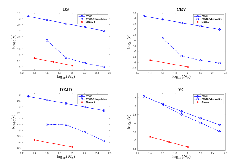
Figure 1: $\log_{10}(\epsilon)$ vs. $\log_{10}(N_{x})$ for evaluating $P_{x,y}(\tau_{a}<\widehat{\tau}_{b}\wedge T)$ under different models.

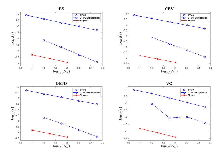
Figure 2: $\log_{10}(\epsilon)$ vs. $\log_{10}({N_{x}})$ for evaluating $\mathbb{E}_{x}\Big{[}e^{-r_{f}\tau_{a}}\mathbf{1}_{\{\int_{0}^{\tau_{a}}\mathbf{1}_{\{X_{s}<\xi\}}\mathop{}\!\mathrm{d}s<T\}}\Big{]}$ under different models.

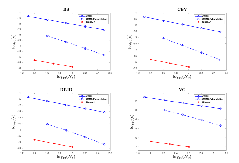
Figure 3: $\log_{10}(\epsilon)$ vs. $\log_{10}(N_{x})$ for evaluating $\mathbb{E}_{x}\Big{[}e^{-r_{f}\tau_{a}}\mathbf{1}_{\{\int_{0}^{\tau_{a}}\mathbf{1}_{\{\overline{X}_{s}-X_{s}>\xi\}}\mathop{}\!\mathrm{d}s<T\}}\Big{]}$ under different models.

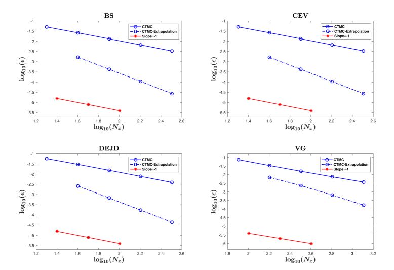
Figure 4: $\log_{10}(\epsilon)$ vs. $\log_{10}(N_{x})$ for evaluating $\sum_{k=1}^{\infty}\mathbb{E}_{x}\Big{[}e^{-r_{f}\tilde{\tau}_{a,k}}\mathbf{1}_{\{\tilde{\tau}_{a,k}<T\}}\Big{]}$ under different models.

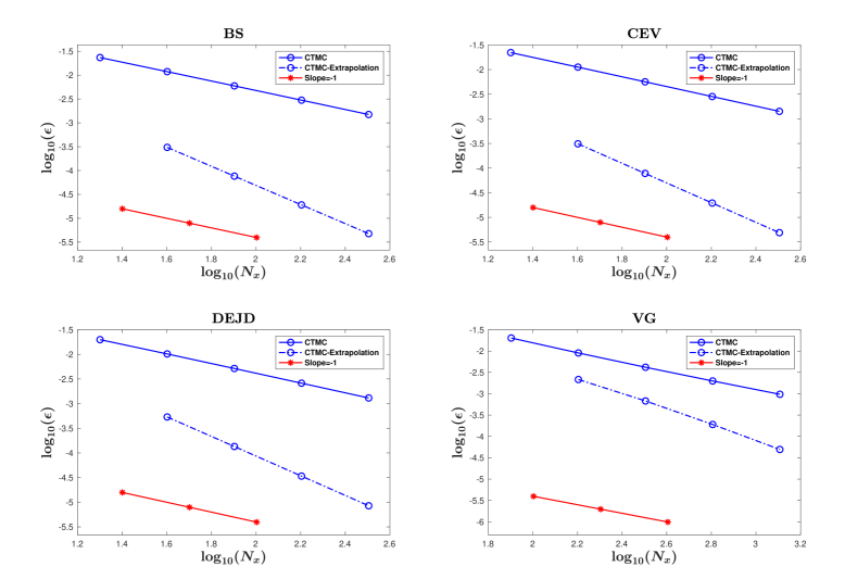
Figure 5: $\log_{10}(\epsilon)$ vs. $\log_{10}(N_{x})$ for evaluating $\mathbb{E}\left[e^{-r_{f}\tau_{a,k}}\mathbf{1}_{\{\tau_{a,k}<T\}}\,\Big{|}\,X_{0}=x,\overline{X}_{0}=y\right]$ under different models.

6 Conclusions

In this paper, we propose a unified framework for computing five important drawdown quantities under general Markov models. Utilizing the CTMC approximation, we derive linear systems for the associated quantities defined under the CTMC and develop algorithms to solve these systems. In particular, by exploiting the inherent spatial homogeneity of Lévy models and birth-death characteristic of diffusion models, we construct more efficient algorithms under these two types of models for a majority of quantities. Notably, we circumvent the challenge posed by highly path-dependent quantities and conduct rigorous convergence analysis of our algorithms under mild conditions. Extensive numerical experiments are presented to demonstrate the good performance of our algorithms. Specifically, in most cases, our algorithms achieve remarkable accuracy with relative errors below 1% within just a few seconds. Even in the worst case, the CPU time remains under 30 seconds. The accuracy can be further enhanced with the aid of the extrapolation technique.

For future research, we can extend our framework in two directions. First, we can consider more complex quantities involving both drawdowns and drawups simultaneously, such as the drawdown time $\tau_{a}$ preceding the drawup time $\tau_{b}$ under a more complicated case $b<a$, as discussed in Remark 4. Second, model assumptions can be generalized beyond Markovian models to incorporate non-Markovian models including rough stochastic local volatility models. The CTMC approximation for rough stochastic local volatility models was constructed in Yang et al. (2025).

Availability of Data and Materials

The datasets generated during and/or analyzed during the current study are available from the corresponding author on reasonable request.

Declarations

We have no conflicts of interest to disclose.

Appendix A Construction of the CTMC Approximation

This section is devoted to constructing a CTMC $Y$ with the state space $\mathbb{S}$ to approximate a Markov process $X$ whose infinitesimal generator $\mathcal{L}$ is depicted in (1). It suffices to specify the transition rate matrix $\bm{G}$ with elements $G(x,y)$ for $x,y\in\mathbb{S}$, such that the infinitesimal generator $\mathcal{G}$ of $Y$ is an approximation of $\mathcal{L}$ in the sense that:

$$\mathcal{G}g(x)\approx\mathcal{L}g(x)$$ (42)

for any function $g\in C^{2}_{c}(I):I\to\mathbb{R}$ and any $x\in\mathbb{S}$.

To this end, the derivative terms and the integral term in (1) are approximated by the central difference method and a summation over the discrete state space $\mathbb{S}$, respectively. More specifically, the derivative terms are approximated as follows:

$$g^{\prime\prime}(x) \approx\Delta g(x):=\frac{\nabla^{+}g(x)-\nabla^{-}g(x)}{\delta x},$$ (43)

$$g^{\prime}(x) \approx\nabla g(x):=\frac{\delta^{-}x}{2\delta x}\nabla^{+}g(x)+\frac{\delta^{+}x}{2\delta x}\nabla^{-}g(x),$$ (44)

where

$$x^{+}=\inf\{y\in\mathbb{S}:y>x\},~\delta^{+}x=x^{+}-x,\qquad x\in\mathbb{S}\backslash\{y_{N}\},$$ (45)

$$x^{-}=\sup\{y\in\mathbb{S}:y<x\},~\delta^{-}x=x-x^{-},\qquad x\in\mathbb{S}\backslash\{y_{0}\},$$ (46)

$$\delta x=\frac{\delta^{+}x+\delta^{-}x}{2},\qquad x\in\mathbb{S}\backslash\{y_{0},y_{N}\},$$ (47)

$$\nabla^{\pm}g(x)=\pm\frac{g(x^{\pm})-g(x)}{\delta^{\pm}x},\qquad x\in\mathbb{S}\backslash\{y_{0},y_{N}\}.$$ (48)

On the other hand, the integral term is approximated as follows:

$$\int_{\mathbb{R}}\big{(}g(x+y)-g(x)-yg^{\prime}(x)\mathbf{1}_{\{|y|\leq 1\}}\big{)}\nu(x,\mathop{}\!\mathrm{d}y)$$ (49)

$$\approx~\frac{1}{2}g^{\prime\prime}(x)\int_{-\delta^{-}x/2}^{\delta^{+}x/2}y^{2}\nu(x,\mathop{}\!\mathrm{d}y)-g^{\prime}(x)\int_{\mathbb{R}\backslash[-\delta^{-}x/2,\delta^{+}x/2]}y\mathbf{1}_{\{|y|\leq 1\}}\nu(x,\mathop{}\!\mathrm{d}y)$$ (50)

$$~~~~+\sum_{z\in\mathbb{S}\backslash\{x\}}\big{(}g(z)-g(x)\big{)}\int^{z+\delta^{+}z/2-x+\infty\mathbf{1}_{\{z=y_{N}\}}}_{z-\delta^{-}z/2-x-\infty\mathbf{1}_{\{z=y_{0}\}}}\nu(x,\mathop{}\!\mathrm{d}y),$$ (51)

where the first term approximates the integral for small jumps and the resulting $g^{\prime\prime}(x)$ is then discretized by the central difference approximation as before.

For brevity, we introduce

$$\overline{b}(x)=\int_{\mathbb{R}\backslash[-\delta^{-}x/2,\delta^{+}x/2]}y\mathbf{1}_{\{|y|\leq 1\}}\nu(x,\mathop{}\!\mathrm{d}y),$$ (52)

$$\overline{\sigma}^{2}(x)=\frac{1}{2}\int_{-\delta^{-}x/2}^{\delta^{+}x/2}y^{2}\nu(x,\mathop{}\!\mathrm{d}y),$$

$$\overline{\nu}(x,z)=\int^{z+\delta^{+}z/2-x+\infty 1_{\{z=y_{N}\}}}_{z-\delta^{-}z/2-x-\infty 1_{\{z=y_{0}\}}}\nu(x,\mathop{}\!\mathrm{d}y).$$

Thus, the infinitesimal generator $\mathcal{G}$ of $Y$ can be chosen as follows: for $x\in\mathbb{S}\backslash\{y_{0},y_{N}\}$,

$$\mathcal{G}g(x)=\frac{1}{2}\big{(}\sigma^{2}(x)+\overline{\sigma}^{2}(x)\big{)}\Delta g(x)+\big{(}b(x)-\overline{b}(x)\big{)}\nabla g(x)+\sum_{z\in\mathbb{S}\backslash\{x\}}\overline{\nu}(x,z)\big{(}g(z)-g(x)\big{)},$$ (53)

otherwise, $\mathcal{G}g(x)=0.$ The generator $\mathcal{G}$ implies that the transition rate matrix $G$ satisfies the following conditions:

$$G(x,x^{+})=(b(x)-\overline{b}(x))\frac{\delta^{-}x}{2\delta^{+}x\delta x}+\frac{1}{2}\big{(}\sigma^{2}(x)+\overline{\sigma}^{2}(x)\big{)}\frac{1}{\delta^{+}x\delta x}+\overline{\nu}(x,x^{+}),~~~~~~x\in\mathbb{S}\backslash\{y_{0},y_{N}\},$$ (54)

$$G(x,x^{-})=-(b(x)-\overline{b}(x))\frac{\delta^{+}x}{2\delta^{-}x\delta x}+\frac{1}{2}\big{(}\sigma^{2}(x)+\overline{\sigma}^{2}(x)\big{)}\frac{1}{\delta^{-}x\delta x}+\overline{\nu}(x,x^{-}),~~~~x\in\mathbb{S}\backslash\{y_{0},y_{N}\},$$ (55)

$$G(x,z)=\overline{\nu}(x,z),~~~~~~~~~~~~~~~~~~~x\in\mathbb{S}\backslash\{y_{0},y_{N}\},~z\in\mathbb{S}\backslash\{x,x^{+},x^{-}\},$$ (56)

$$G(x,x)=-\sum_{y\in\mathbb{S}\backslash\{x\}}G(x,y),\qquad x\in\mathbb{S},$$ (57)

and all other elements of $G$ are zeros.

Remark 13.

For Lévy processes, it is desirable to construct a CTMC that preserves the property of independent and stationary increments. To this end, a CTMC $Y$ with the state space $\mathbb{S}=h\mathbb{Z}$ is chosen to approximate the Lévy process $X$ so that $Y$ itself is also a Lévy process. Here, $h>0$ and $\mathbb{Z}$ denotes the set of integers. In this case, for any $x\in\mathbb{S}$, we have $x^{\pm}=x\pm h$ and $\delta^{\pm}x=\delta x=h.$ Moreover, $b(x),~\sigma^{2}(x),$ and $\nu(x,\mathop{}\!\mathrm{d}y)$ in (1) are independent of $x$, which enables us to write $b=b(x),$ $\sigma^{2}=\sigma^{2}(x),$ and $\nu(\mathop{}\!\mathrm{d}y)=\nu(x,\mathop{}\!\mathrm{d}y)$. Therefore, we introduce $\overline{b}=\int_{\mathbb{R}\backslash[-h/2,h/2]}y\mathbf{1}_{\{|y|\leq 1\}}\nu(\mathop{}\!\mathrm{d}y),$ $\overline{\sigma}^{2}=\frac{1}{2}\int_{-h/2}^{h/2}y^{2}\nu(\mathop{}\!\mathrm{d}y),$ and $\overline{\nu}(z-x)=\int^{z-x+h/2}_{z-x-h/2}\nu(\mathop{}\!\mathrm{d}y)$. It follows that the transition rate matrix $G$ is characterized by

$$G(x,x+h)=\frac{b-\overline{b}}{2h}+\frac{\sigma^{2}+\overline{\sigma}^{2}}{2h^{2}}+\overline{\nu}(h),$$ (58)

$$G(x,x-h)=-\frac{b-\overline{b}}{2h}+\frac{\sigma^{2}+\overline{\sigma}^{2}}{2h^{2}}+\overline{\nu}(-h),$$ (59)

$$G(x,z)=\overline{\nu}(z-x),~~~~z\in\mathbb{S}\backslash\{x,~x\pm h\},$$ (60)

$$G(x,x)=-\sum_{y\in\mathbb{S}\backslash\{x\}}G(x,y).$$ (61)

Remark 14.

For diffusion processes, we have $\overline{b}(x)=0$, $\overline{\sigma}^{2}(x)=0$, and $\overline{\nu}(x,z)=0$ for all $x,z\in\mathbb{S}$. The resulting CTMC is a birth-death process.

Appendix B Proofs

B.1 Proof of Proposition 1

Proof.

Similar to the proof of Theorem 3.1 in Zhang and Li (2023c), by the introduction of $T_{x}^{+}$, $A(q,x,y)$ can be decomposed as follows:

$$A(q,x,y)=\mathbb{E}_{x,y}\big{[}e^{-q\tau_{a}}\mathbf{1}_{\{\tau_{a}<\widehat{\tau}_{b},\,\tau_{a}<T_{x}^{+}\}}f(Y_{\tau_{a}})\big{]}+\mathbb{E}_{x,y}\big{[}e^{-q\tau_{a}}\mathbf{1}_{\{\tau_{a}<\widehat{\tau}_{b},\,\tau_{a}>T_{x}^{+}\}}f(Y_{\tau_{a}})\big{]}.$$ (62)

On the event $\{\tau_{a}<T_{x}^{+}\}$, we have $\tau_{a}=T_{x-a}^{-}$ and the drawup up to $\tau_{a}$ is less than $b$, leading to $\tau_{a}<\widehat{\tau}_{b}$. On the other hand, notice that $\{\tau_{a}>T_{x}^{+}\}=\{T_{x-a}^{-}>T_{x}^{+}\}$. Therefore, for $x\in\mathbb{S}$ and $y\in\mathbb{S}\cap(x-a,x]$, we have

$$A(q,x,y)$$ (63)

$$=\mathbb{E}_{x,y}\big{[}e^{-qT_{x-a}^{-}}\mathbf{1}_{\{T_{x-a}^{-}<T_{x}^{+}\}}f(Y_{T_{x-a}^{-}})\big{]}$$ (64)

$$~~~~+\mathbb{E}_{x,y}\big{[}e^{-qT_{x}^{+}}\mathbf{1}_{\{T_{x-a}^{-}>T_{x}^{+}\}}\mathbb{E}[e^{-q(\tau_{a}-T_{x}^{+})}\mathbf{1}_{\{\tau_{a}<\widehat{\tau}_{b}\}}f(Y_{\tau_{a}})\,|\,Y_{T_{x}^{+}},\overline{Y}_{T_{x}^{+}}=Y_{T_{x}^{+}},\underline{Y}_{T_{x}^{+}}]\big{]}$$ (65)

$$=P_{(x-a,x]}(q,x;f(\cdot)\mathbf{1}_{\{\cdot\leq x-a\}})+\mathbb{E}_{x,y}\big{[}e^{-qT_{x}^{+}}\mathbf{1}_{\{T_{x-a}^{-}>T_{x}^{+}\}}A(q,Y_{T_{x}^{+}},\underline{Y}_{T_{x}^{+}})\big{]}$$ (66)

$$=P_{(x-a,x]}(q,x;f(\cdot)\mathbf{1}_{\{\cdot\leq x-a\}})$$ (67)

$$~~~~+\sum_{z\in\mathbb{S}\cap(x,y+b),\,{w\in\mathbb{S}\cap((x-a)\vee(z-b),y]}}\mathbb{E}_{x,y}\big{[}e^{-qT_{x}^{+}}\mathbf{1}_{\{T_{x-a}^{-}>T_{x}^{+},\,Y_{T_{x}^{+}}=z,\,\underline{Y}_{Y_{x}^{+}}=w\}}A(q,Y_{T_{x}^{+}},\underline{Y}_{T_{x}^{+}})\big{]}$$ (68)

$$=P_{(x-a,x]}(q,x;f(\cdot)\mathbf{1}_{\{\cdot\leq x-a\}})$$ (69)

$$~~~~+\sum_{z\in\mathbb{S}\cap(x,y+b),\,{w\in\mathbb{S}\cap((x-a)\vee(z-b),y]}}\mathbb{E}_{x,y}\big{[}e^{-qT_{x}^{+}}\mathbf{1}_{\{T_{x-a}^{-}>T_{x}^{+},\,Y_{T_{x}^{+}}=z,\,\underline{Y}_{Y_{x}^{+}}=w\}}\big{]}A(q,z,w),$$ (70)

which in conjunction with the definition of the quantity $R_{(\ell,r]}(q,x,y;g)$ yields (14).

It remains to derive the linear system for the quantity $R_{(\ell,r]}(q,x,y;g)$. For $x\leq\ell$, we have $\{T_{r}^{+}<T_{\ell}^{-}\}=\emptyset$, leading to $R_{(\ell,r]}(q,x,y;g)=0$, while for $x>r$, we have $T_{r}^{+}=0$, resulting in $R_{(\ell,r]}(q,x,y;g)=g(x,y)$. Consider $x\in(\ell,r]$, inspired by the proof of Proposition 3.1 in Zhang and Li (2023c), we introduce $\mathbb{T}_{t}=\{kt:k=0,1,\dots\}$ and define $\mathbb{T}_{(\ell,r]}=\inf\{s\in\mathbb{T}_{t}:Y_{s}\notin(\ell,r]\},~\mathbb{T}_{r}^{+}=\mathbb{T}_{(-\infty,r]},$ and $\mathbb{T}_{\ell}^{-}=\mathbb{T}_{(\ell,\infty)}$. The Markov property of $Y$ yields

$$\mathbb{E}\big{[}e^{-q\mathbb{T}_{r}^{+}}\mathbf{1}_{\{\mathbb{T}_{\ell}^{-}>\mathbb{T}_{r}^{+}\}}g(Y_{\mathbb{T}_{r}^{+}},\underline{Y}_{\mathbb{T}_{r}^{+}})\,\big{|}\,Y_{0}=x,\underline{Y}_{0}=y\big{]}$$

$$=e^{-qt}\sum_{z\in\mathbb{S}}\mathbb{E}\big{[}e^{-q\mathbb{T}_{r}^{+}}\mathbf{1}_{\{\mathbb{T}_{\ell}^{-}>\mathbb{T}_{r}^{+}\}}g(Y_{\mathbb{T}_{r}^{+}},\underline{Y}_{\mathbb{T}_{r}^{+}})\,\big{|}\,Y_{0}=z,\underline{Y}_{0}=y\wedge z\big{]}p(t,x,z)$$

$$=(1-qt)t\sum_{z\in\mathbb{S},\,z\neq x}\mathbb{E}\big{[}e^{-q\mathbb{T}_{r}^{+}}\mathbf{1}_{\{\mathbb{T}_{\ell}^{-}>\mathbb{T}_{r}^{+}\}}g(Y_{\mathbb{T}_{r}^{+}},\underline{Y}_{\mathbb{T}_{r}^{+}})\,\big{|}\,Y_{0}=z,\underline{Y}_{0}=y\wedge z\big{]}G(x,z)$$

$$~~~~+(1-qt)\mathbb{E}\big{[}e^{-q\mathbb{T}_{r}^{+}}\mathbf{1}_{\{\mathbb{T}_{\ell}^{-}>\mathbb{T}_{r}^{+}\}}g(Y_{\mathbb{T}_{r}^{+}},\underline{Y}_{\mathbb{T}_{r}^{+}})\,\big{|}\,Y_{0}=x,\underline{Y}_{0}=y\big{]}(1+G(x,x)t)+o(t),$$

where $p(t,x,z):=P(Y_{t}=z\,|\,Y_{0}=x)$. The second equality holds since $p(t,x,z)=\mathbf{1}_{\{x=z\}}+G(x,z)t+o(t)$ and $e^{-qt}=1-qt+o(t)$ when $t\to 0$. Dividing both sides by $t$ gives

$$\sum_{z\in\mathbb{S}}G(x,z)\mathbb{E}\big{[}e^{-q\mathbb{T}_{r}^{+}}\mathbf{1}_{\{\mathbb{T}_{r}^{+}<\mathbb{T}_{\ell}^{-}\}}g(Y_{\mathbb{T}_{r}^{+}},\underline{Y}_{\mathbb{T}_{r}^{+}})\,\big{|}\,Y_{0}=z,\underline{Y}_{0}=y\wedge z\big{]}$$

$$-q\mathbb{E}\big{[}e^{-q\mathbb{T}_{r}^{+}}\mathbf{1}_{\{\mathbb{T}_{r}^{+}<\mathbb{T}_{\ell}^{-}\}}g(Y_{\mathbb{T}_{r}^{+}},\underline{Y}_{\mathbb{T}_{r}^{+}})\,\big{|}\,Y_{0}=x,\underline{Y}_{0}=y\big{]}+o(1)=0.$$

By similar arguments in the proof of Proposition 3.1 in Zhang and Li (2023c), we finally arrive at (16). ∎

B.2 Proof of Proposition 2

Proof.

Recall that on the event $\{\tau_{a}<T_{x}^{+}\}$, we have $\tau_{a}=T_{x-a}^{-}$. Moreover, $\{\tau_{a}>T_{x}^{+}\}=\{T_{x-a}^{-}>T_{x}^{+}\}$. Thus,

$$B(k,x)=~ \mathbb{E}_{x}\Big{[}e^{-\int_{0}^{\tau_{a}}k(Y_{s})\mathop{}\!\mathrm{d}s}\mathbf{1}_{\{\tau_{a}<T_{x}^{+}\}}f(Y_{\tau_{a}})\Big{]}+\mathbb{E}_{x}\Big{[}e^{-\int_{0}^{\tau_{a}}k(Y_{s})\mathop{}\!\mathrm{d}s}\mathbf{1}_{\{\tau_{a}>T_{x}^{+}\}}f(Y_{\tau_{a}})\Big{]}$$ (71)

$$=~ \mathbb{E}_{x}\Big{[}e^{-\int_{0}^{T_{x-a}^{-}}k(Y_{s})\mathop{}\!\mathrm{d}s}\mathbf{1}_{\{T_{x-a}^{-}<T_{x}^{+}\}}f(Y_{T_{x-a}^{-}})\Big{]}$$ (72)

$$+\sum_{z\in\mathbb{S},\,z>x}\mathbb{E}_{x}\Big{[}e^{-\int_{0}^{T_{x}^{+}}k(Y_{s})\mathop{}\!\mathrm{d}s}\mathbf{1}_{\{T_{x-a}^{-}>T_{x}^{+},\,Y_{T_{x}^{+}}=z\}}B(k,Y_{T_{x}^{+}})\Big{]}$$ (73)

$$=~ P_{(x-a,x]}(k,x;f(\cdot)\mathbf{1}_{\{\cdot\leq x-a\}})+\sum_{z\in\mathbb{S},\,z>x}\mathbb{E}_{x}\Big{[}e^{-\int_{0}^{T_{x}^{+}}k(Y_{s})\mathop{}\!\mathrm{d}s}\mathbf{1}_{\{T_{x-a}^{-}>T_{x}^{+},\,Y_{T_{x}^{+}}=z\}}\Big{]}B(k,z)$$ (74)

$$=~ P_{(x-a,x]}(k,x;f(\cdot)\mathbf{1}_{\{\cdot\leq x-a\}})+\sum_{z\in\mathbb{S},\,z>x}P_{(x-a,x]}(k,x;\mathbf{1}_{\{\cdot=z\}})B(k,z).$$ (75)

∎

B.3 Proof of Proposition 3

Proof.

Using similar arguments in the proof of Proposition 2, we have

$$C(k,x)=~ \mathbb{E}_{x}\Big{[}e^{-\int_{0}^{\tau_{a}}k(Y_{s},\overline{Y}_{s})\mathop{}\!\mathrm{d}s}\mathbf{1}_{\{\tau_{a}<T_{x}^{+}\}}f(Y_{\tau_{a}})\Big{]}+\mathbb{E}_{x}\Big{[}e^{-\int_{0}^{\tau_{a}}k(Y_{s},\overline{Y}_{s})\mathop{}\!\mathrm{d}s}\mathbf{1}_{\{\tau_{a}>T_{x}^{+}\}}f(Y_{\tau_{a}})\Big{]}$$ (76)

$$=~ \mathbb{E}_{x}\Big{[}e^{-\int_{0}^{T_{x-a}^{-}}k(Y_{s},\overline{Y}_{s})\mathop{}\!\mathrm{d}s}\mathbf{1}_{\{T_{x-a}^{-}<T_{x}^{+}\}}f(Y_{T_{x-a}^{-}})\Big{]}$$ (77)

$$+\sum_{z\in\mathbb{S},\,z>x}\mathbb{E}_{x}\Big{[}e^{-\int_{0}^{T_{x}^{+}}k(Y_{s},\overline{Y}_{s})\mathop{}\!\mathrm{d}s}\mathbf{1}_{\{T_{x-a}^{-}>T_{x}^{+},\,Y_{T_{x}^{+}}=z\}}C(k,Y_{T_{x}^{+}})\Big{]}$$ (78)

$$=~ P_{(x-a,x]}(k(\cdot,x),x;f(\cdot)\mathbf{1}_{\{\cdot\leq x-a\}})$$ (79)

$$+\sum_{z\in\mathbb{S},\,z>x}\mathbb{E}_{x}\Big{[}e^{-\int_{0}^{T_{x}^{+}}k(Y_{s},\overline{Y}_{s})\mathop{}\!\mathrm{d}s}\mathbf{1}_{\{T_{x-a}^{-}>T_{x}^{+},\,Y_{T_{x}^{+}}=z\}}\Big{]}C(k,z)$$ (80)

$$=~ P_{(x-a,x]}(k(\cdot,x),x;f(\cdot)\mathbf{1}_{\{\cdot\leq x-a\}})+\sum_{z\in\mathbb{S},\,z>x}S_{(x-a,x]}(k,x,x;\mathbf{1}_{\{\cdot=z\}})C(k,z).$$ (81)

The linear system for the quantity $S_{(\ell,r]}(k,x,y;g)$ can be derived in a similar way as the quantity $R_{(\ell,r]}(q,x,y;g)$ (see the proof of Proposition 1) and hence is omitted here. ∎

B.4 Proof of Proposition 4

Proof.

Applying the law of iterated expectations and Lemma 2 yields

$$H_{n}(q,x)= ~\mathbb{E}_{x}\Big{[}e^{-q\tilde{\tau}_{a,n}}f(Y_{\tilde{\tau}_{a,n}})\Big{]}$$

$$= ~\mathbb{E}_{x}\Big{[}e^{-q\tilde{\tau}_{a,1}}\mathbb{E}\big{[}e^{-q(\tilde{\tau}_{a,n}-\tilde{\tau}_{a,1})}f(Y_{\tilde{\tau}_{a,n}})\,|\,Y_{\tilde{\tau}_{a,1}},\overline{Y}_{\tilde{\tau}_{a,1},\tilde{\tau}_{a,1}}\big{]}\Big{]}$$

$$= ~\mathbb{E}_{x}\Big{[}e^{-q\tilde{\tau}_{a,1}}H_{n-1}(q,Y_{\tilde{\tau}_{a,1}})\Big{]}$$

$$= ~Q_{a}(q,x;H_{n-1}(q,\cdot))$$

$$= ~P_{(x-a,x]}(q,x;H_{n-1}(q,\cdot)\mathbf{1}_{\{\cdot\leq x-a\}})+\sum_{y\in\mathbb{S},\,y>x}P_{(x-a,x]}\big{(}q,x;\mathbf{1}_{\{\cdot=y\}}\big{)}H_{n}(q,y).$$

∎

B.5 Proof of Proposition 5

Proof.

Since $\tau_{a,n}>T_{(-\infty,y)}$ and $\overline{Y}_{T_{(-\infty,y)}}=Y_{T_{(-\infty,y)}}\geq y$, applying the law of iterated expectations yields

$$J_{n}(q,x,y) =\mathbb{E}\Big{[}e^{-qT_{(-\infty,y)}}\mathbb{E}\big{[}e^{-q(\tau_{a,n}-T_{(-\infty,y)})}f(Y_{\tau_{a,n}},\overline{Y}_{\tau_{a,n}})\,\big{|}\,Y_{T_{(-\infty,y)}},\overline{Y}_{T_{(-\infty,y)}}\big{]}\,\Big{|}\,Y_{0}=x,\overline{Y}_{0}=y\Big{]}$$

$$=\mathbb{E}\Big{[}e^{-qT_{(-\infty,y)}}J_{n}(q,Y_{T_{(-\infty,y)}},Y_{T_{(-\infty,y)}})\,\big{|}\,Y_{0}=x,\overline{Y}_{0}=y\Big{]}$$

$$=\sum_{z\in\mathbb{S},\,z\geq y}P_{(-\infty,y)}(q,x;\mathbf{1}_{\{\cdot=z\}})J_{n}(q,z,z).$$

On the other hand, $J_{n}(q,y,y)$ can be decomposed as follows

$$J_{n}(q,y,y)= ~\mathbb{E}\big{[}e^{-q\tau_{a,n}}f(Y_{\tau_{a,n}},\overline{Y}_{\tau_{a,n}})\,\big{|}\,Y_{0}=y,\overline{Y}_{0}=y\big{]}$$

$$= ~\mathbb{E}\big{[}e^{-q\tau_{a,n}}\mathbf{1}_{\{\tau_{a,1}<T_{y}^{+}\}}f(Y_{\tau_{a,n}},\overline{Y}_{\tau_{a,n}})\,\big{|}\,Y_{0}=y,\overline{Y}_{0}=y\big{]}$$

$$~+\mathbb{E}\big{[}e^{-q\tau_{a,n}}\mathbf{1}_{\{\tau_{a,1}>T_{y}^{+}\}}f(Y_{\tau_{a,n}},\overline{Y}_{\tau_{a,n}})\,\big{|}\,Y_{0}=y,\overline{Y}_{0}=y\big{]}$$

$$= ~\mathbb{E}\Big{[}e^{-q\tau_{a,1}}\mathbf{1}_{\{\tau_{a,1}<T_{y}^{+}\}}\mathbb{E}\big{[}e^{-q(\tau_{a,n}-\tau_{a,1})}f(Y_{\tau_{a,n}},\overline{Y}_{\tau_{a,n}})\,\big{|}\,Y_{\tau_{a,1}},\overline{Y}_{\tau_{a,1}}\big{]}\,\Big{|}\,Y_{0}=y,\overline{Y}_{0}=y\Big{]}$$

$$~+\mathbb{E}\Big{[}e^{-qT_{y}^{+}}\mathbf{1}_{\{\tau_{a,1}>T_{y}^{+}\}}\mathbb{E}\big{[}e^{-q(\tau_{a,n}-T_{y}^{+})}f(Y_{\tau_{a,n}},\overline{Y}_{\tau_{a,n}})\,\big{|}\,Y_{T_{y}^{+}},\overline{Y}_{T_{y}^{+}}\big{]}\,\Big{|}\,Y_{0}=y,\overline{Y}_{0}=y\Big{]}$$

$$= ~\mathbb{E}\Big{[}e^{-qT_{y-a}^{-}}\mathbf{1}_{\{T_{y-a}^{-}<T_{y}^{+}\}}J_{n-1}(q,Y_{T_{y-a}^{-}},y)\,\Big{|}\,Y_{0}=y,\overline{Y}_{0}=y\Big{]}$$

$$~+\sum_{z\in\mathbb{S},\,z>y}\mathbb{E}\Big{[}e^{-qT_{y}^{+}}\mathbf{1}_{\{T_{y-a}^{-}>T_{y}^{+},Y_{T_{y}^{+}}=z\}}J_{n}(q,Y_{T_{y}^{+}},Y_{T_{y}^{+}})\,\Big{|}\,Y_{0}=y,\overline{Y}_{0}=y\Big{]}$$

$$= ~P_{(y-a,y]}(q,y;J_{n-1}(q,\cdot,y)\mathbf{1}_{\{\cdot\leq y-a\}})+\sum_{z\in\mathbb{S},\,z>y}P_{(y-a,y]}(q,y;\mathbf{1}_{\{\cdot=z\}})J_{n}(q,z,z).$$

Here, the sixth line is attributed to the fact that on the event $\{\tau_{a,1}<T_{y}^{+}\}$, we have $\tau_{a,1}=T_{y-a}^{-}$ and $\overline{Y}_{\tau_{a,1}}=\overline{Y}_{0}=y$, and the seventh line holds since the condition $Y_{0}=\overline{Y}_{0}=y$ implies that $Y_{T_{y}^{+}}=\overline{Y}_{T_{y}^{+}}>y$. ∎

B.6 Proof of Theorem 1

Proof.

For brevity, we write $s^{\prime}=\tau_{a}(\omega)$, $s^{\prime(n)}=\tau_{a}(\omega^{(n)})$, $\overline{\omega}_{s,t}^{(n)}=\sup_{u\in[s,t]}\omega_{u}^{(n)}$, $MD_{s,t}=\sup_{u\in[s,t]}(\overline{\omega}_{s,u}-\omega_{u})$, $MD_{s,t}^{(n)}=\sup_{u\in[s,t]}(\overline{\omega}_{s,u}^{(n)}-\omega_{u}^{(n)})$, $M_{k}=\sup_{u\in[\tau_{a,k-1}(\omega),\tau_{a,k}(\omega)]}\omega_{u}$, $M_{k}^{(n)}=\sup_{u\in[\tau_{a,k-1}(\omega^{(n)}),\tau_{a,k}(\omega^{(n)})]}\omega_{u}^{(n)}$, $T_{M_{k}}=\inf\{t>\tau_{a,k}(\omega):\omega_{t}\geq M_{k}\}$, and $T_{M_{k}}^{(n)}=\inf\{t>\tau_{a,k}(\omega^{(n)}):\omega_{t}^{(n)}\geq M_{k}^{(n)}\},$ where $0\leq s<t$ and $k=1,2,\dots$. Define $\tau_{a,0}(\omega)=\tau_{a,0}(\omega^{(n)})=0$. In the subsequent analysis, we focus on establishing the continuity of the mappings w.r.t. the sample path $\omega$. Combined with the weak convergence $Y^{(n)}\Rightarrow X$, this continuity property ensures the quantities defined under the CTMC $Y^{(n)}$ converge in distribution to their counterparts defined under the Markov process $X$.

1. It suffices to show that $\omega\mapsto(\tau_{a}(\omega),\widehat{\tau}_{b}(\omega),\omega_{\tau_{a}(\omega)})$ is a continuous mapping almost surely. Since the continuity of the mapping $\omega\mapsto(\tau_{a}(\omega),\omega_{\tau_{a}(\omega)})$ has been verified by Zhang and Li (2023c), it remains to prove the mapping $\omega\mapsto\widehat{\tau}_{b}(\omega)$ is continuous. Observe that the running minimum satisfies the identity $\inf_{0\leq s\leq t}X_{s}=-\sup_{0\leq s\leq t}(-X_{s})$. Following the methodology of Zhang and Li (2023c, Theorem 4.1), we directly verify the continuity of the mapping $\omega\mapsto\widehat{\tau}_{b}(\omega)$.

2. As discussed above, it suffices to show the continuity of the mapping $\omega\mapsto\int_{0}^{\tau_{a}(\omega)}k(\omega_{s})\mathop{}\!\mathrm{d}s$. Suppose $\omega^{(n)}\to\omega$ under the Skorokhod topology. For any $\epsilon>0$, denote by $\bm{T}_{\epsilon}=\cup_{1\leq i\leq m}(t_{i}-\epsilon,t_{i}+\epsilon)$ the neighbourhood of $\bm{T}_{dis}$. By Jacod and Shiryaev (2013, Chapter VI, Section 2, 2.3), for $s\in(0,\tau_{a})\setminus\bm{T}_{\epsilon}$, the convergence $\omega_{s}^{(n)}\to\omega_{s}$ holds as $n\to\infty$, ensuring the convergence $k(\omega_{s}^{(n)})\to k(\omega_{s})$. Denote by $U_{k}$ the upper bound of the function $k(\cdot)$. Notice that $\tau_{a}(\omega^{(n)})\to\tau_{a}(\omega)$ as $n\to\infty$, then it follows that

   $$\left|\int_{0}^{\tau_{a}(\omega)}k(\omega_{s}^{(n)})\mathop{}\!\mathrm{d}s-\int_{0}^{\tau_{a}(\omega^{(n)})}k(\omega_{s}^{(n)})\mathop{}\!\mathrm{d}s\right|\leq U_{k}\left|\tau_{a}(\omega)-\tau_{a}(\omega^{(n)})\right|\to 0.$$

   On the other hands,

   $$\left|\int_{0}^{\tau_{a}(\omega)}k(\omega_{s})\mathop{}\!\mathrm{d}s-\int_{0}^{\tau_{a}(\omega)}k(\omega_{s}^{(n)})\mathop{}\!\mathrm{d}s\right|$$

   $$\leq\int_{\bm{T}_{\epsilon}}\left|k(\omega_{s})-k(\omega_{s}^{(n)})\right|\mathop{}\!\mathrm{d}s+\int_{(0,\tau_{a}(\omega))\setminus\bm{T}_{\epsilon}}\left|k(\omega_{s})-k(\omega_{s}^{(n)})\right|\mathop{}\!\mathrm{d}s$$

   $$\leq 4mU_{k}\epsilon+\int_{(0,\tau_{a}(\omega))\setminus\bm{T}_{\epsilon}}\left|k(\omega_{s})-k(\omega_{s}^{(n)})\right|\mathop{}\!\mathrm{d}s$$

   $$\to 4mU_{k}\epsilon.$$

   The second inequality is established by the boundedness of the function $k(\cdot)$ and the last line follows from an application of the dominated convergence theorem. Since $\epsilon$ can be arbitrarily small, combining the above two results yields that $\int_{0}^{\tau_{a}(\omega^{(n)})}k(\omega_{s}^{(n)})\mathop{}\!\mathrm{d}s\to\int_{0}^{\tau_{a}(\omega)}k(\omega_{s})\mathop{}\!\mathrm{d}s$ as $n\to\infty$.

3. The proof of the continuity of the mapping $\omega\mapsto\int_{0}^{\tau_{a}(\omega)}k(\omega_{s},\overline{\omega}_{s})\mathop{}\!\mathrm{d}s$ is analogous to that of the mapping $\omega\mapsto\int_{0}^{\tau_{a}(\omega)}k(\omega_{s})\mathop{}\!\mathrm{d}s$ and hence is omitted.

4. According to Zhang and Li (2023c, Theorem 4.1), $\tilde{\tau}_{a,1}(\omega^{(n)})=\tau_{a}(\omega^{(n)})\to\tau_{a}(\omega)=\tilde{\tau}_{a,1}(\omega)$ as $n\to\infty$. Therefore, it suffices to show the continuity of the mapping $\omega\mapsto\tilde{\tau}_{a,2}(\omega)$, and the continuity of the mappings $\omega\mapsto\tilde{\tau}_{a,k}$ for $k=3,\dots$ can be proved by mathematical induction.

   Assume $s^{\prime}<\tilde{\tau}_{a,2}(\omega)<s,~\omega\in U$, and $s\in\mathbb{R}^{+}\setminus J(\omega)$, then $MD_{s^{\prime},s}>a$. By the right-continuity of the path $\omega$ at $s^{\prime}$, $MD_{s^{\prime},s}$ inherits this property and is also right-continuous at $s^{\prime}$. Consequently, there exists a $\delta\in(0,s-s^{\prime})$ such that $s^{\prime}+\delta\in\mathbb{R}^{+}\setminus J(\omega)$ and $MD_{s^{\prime}+\delta,s}>a$. Zhang and Li (2023c, Theorem 4.1) implies that $MD_{s^{\prime}+\delta,s}^{(n)}\to MD_{s^{\prime}+\delta,s}$ as $n\to\infty$, in conjunction with the previous result yields $MD_{s^{\prime}+\delta,s}^{(n)}>a$ for a sufficiently large $n$. Since $s^{\prime(n)}\to s^{\prime}$, for a sufficiently large $n$, it follows that $s^{\prime(n)}\leq s^{\prime}+\delta$ and hence $MD_{s^{\prime(n)},s}^{(n)}\geq MD_{s^{\prime}+\delta,s}^{(n)}>a$, equivalently, $\tilde{\tau}_{a,2}(\omega^{(n)})<s$. The arbitrariness of $s$ and dense property of the set $\mathbb{R}^{+}\setminus J(\omega)$ finally result in $\lim\sup_{n\to\infty}\tilde{\tau}_{a,2}(\omega^{(n)})\leq\tilde{\tau}_{a,2}(\omega)$.

   Suppose $s^{\prime}<s<\tilde{\tau}_{a,2}(\omega)$, $\omega\in\widetilde{\mathcal{W}}$, and $s\in\mathbb{R}^{+}\setminus J(\omega)$, then $MD_{s^{\prime},s}<a$. Moreover, there exists a $\delta\in(0,s^{\prime})$ such that $MD_{s^{\prime}-\delta,s}<a$. The convergence $s^{\prime(n)}\to s^{\prime}$ implies that $s^{\prime(n)}>s^{\prime}-\delta$ holds for a sufficiently large $n$. Furthermore, applying Zhang and Li (2023c, Theorem 4.1) yields $\lim_{n\to\infty}MD_{s^{\prime(n)},s}^{(n)}\leq\lim_{n\to\infty}MD_{s^{\prime}-\delta,s}^{(n)}=MD_{s^{\prime}-\delta,s}<a$, equivalently, $\tilde{\tau}_{a,2}(\omega^{(n)})>s$. As $s$ is arbitrary and $\mathbb{R}^{+}\setminus J(\omega)$ is dense, it follows that $\lim\inf_{n\to\infty}\tilde{\tau}_{a,2}(\omega^{(n)})\geq\tilde{\tau}_{a,2}(\omega)$.

   Combining the above two results concludes the proof.

5. Following the above proof of conclusion (4) in Theorem 1, it suffices to prove the continuity of the mapping of $\omega\mapsto\tau_{a,2}(\omega)$. Observe that $\tau_{a,2}(\omega)=T_{M_{1}}+\inf\{t>T_{M_{1}}:\overline{\omega}_{T_{M_{1}},t}-X_{t}\geq a\}$ and $\tau_{a,2}(\omega^{(n)})=T_{M_{1}}^{(n)}+\inf\{t>T_{M_{1}}^{(n)}:\overline{\omega}_{T_{M_{1}}^{(n)},t}^{(n)}-Y_{t}^{(n)}\geq a\}$. It remains to show the convergence of $T_{M_{1}}^{(n)}$ as the convergence of the second term involved in $\tau_{a,2}(\omega^{(n)})$ can be proved in a similar way as that of $\tilde{\tau}_{a,2}(\omega^{(n)})$.

   Suppose $s^{\prime}<T_{M_{1}}<s,~\omega\in{V}$, and $s\in\mathbb{R}^{+}\setminus J(\omega)$. Thus, $\overline{\omega}_{0,s^{\prime}}<\overline{\omega}_{s^{\prime},s}$. By the right-continuity of the path $\omega$ at $s^{\prime}$, there exists a $\delta\in(0,s-s^{\prime})$ such that $s^{\prime}+\delta\in\mathbb{R}^{+}\setminus J(\omega)$ and $\overline{\omega}_{s^{\prime},s^{\prime}+\delta}<\overline{\omega}_{s^{\prime}+\delta,s}$. On the other hand, applications of Song et al. (2013, Lemma 6) and Jacod and Shiryaev (2013, Chapter VI, Section 2, 2.3) yield $\overline{\omega}_{0,s^{\prime}+\delta}^{(n)}\to\overline{\omega}_{0,s^{\prime}+\delta}$ and $\overline{\omega}_{s^{\prime}+\delta,s}^{(n)}\to\overline{\omega}_{s^{\prime}+\delta,s}$ as $n\to\infty$. Besides, since $s^{\prime(n)}\to s^{\prime}$, for a sufficiently large $n$, it follows that $s^{\prime(n)}<s^{\prime}+\delta$. As a result, $\lim_{n\to\infty}\overline{\omega}_{0,s^{\prime(n)}}^{(n)}\leq\lim_{n\to\infty}\overline{\omega}_{0,s^{\prime}+\delta}^{(n)}=\overline{\omega}_{0,s^{\prime}+\delta}<\overline{\omega}_{s^{\prime}+\delta,s}=\lim_{n\to\infty}\overline{\omega}_{s^{\prime}+\delta,s}^{(n)}\leq\lim_{n\to\infty}\overline{\omega}_{s^{\prime(n)},s}^{(n)}$, equivalently, $s^{\prime(n)}<T_{M_{1}}^{(n)}<s$. Finally, by the arbitrariness of $s$ and dense property of the set $\mathbb{R}^{+}\setminus J(\omega)$, the inequality $\lim\sup_{n\to\infty}T_{M_{1}}^{(n)}\leq T_{M_{1}}$ holds.

   Suppose $s^{\prime}<s<T_{M_{1}}$, $\omega\in\mathcal{W}$, and $s\in\mathbb{R}^{+}\setminus J(\omega)$, then $\overline{\omega}_{0,s^{\prime}}>\overline{\omega}_{s^{\prime},s}$. Moreover, there exists a $\delta>0$ such that $s^{\prime}-\delta\in\mathbb{R}^{+}\setminus J(\omega)$ and $\overline{\omega}_{0,s^{\prime}-\delta}>\overline{\omega}_{s^{\prime}-\delta,s}$. On the other hand, applying Song et al. (2013, Lemma 6) and Jacod and Shiryaev (2013, Chapter VI, Section 2, 2.3) yield $\lim_{n\to\infty}\overline{\omega}_{0,s^{\prime}-\delta}^{(n)}=\overline{\omega}_{0,s^{\prime}-\delta}$ and $\lim_{n\to\infty}\overline{\omega}_{s^{\prime}-\delta,s}^{(n)}=\overline{\omega}_{s^{\prime}-\delta,s}$. Besides, the convergence $s^{\prime(n)}\to s^{\prime}$ implies that $s^{\prime(n)}>s^{\prime}-\delta$ for a sufficiently large $n$. As a result, $\lim_{n\to\infty}\overline{\omega}_{0,s^{\prime(n)}}^{(n)}\geq\lim_{n\to\infty}\overline{\omega}_{0,s^{\prime}-\delta}^{(n)}=\overline{\omega}_{0,s^{\prime}-\delta}>\overline{\omega}_{s^{\prime}-\delta,s}=\lim_{n\to\infty}\overline{\omega}_{s^{\prime}-\delta,s}^{(n)}\geq\lim_{n\to\infty}\overline{\omega}_{s^{\prime(n)},s}^{(n)}$, equivalently, $T_{M_{1}}^{(n)}>s$. The arbitrariness of $s$ and dense property of the set $\mathbb{R}^{+}\setminus J(\omega)$ finally lead to $\lim\inf_{n\to\infty}T_{M_{1}}^{(n)}\geq T_{M_{1}}$.

   Combining the above two results completes the proof.

∎

References

• Abate and Whitt (1992) Abate, J. and W. Whitt (1992). The Fourier-series method for inverting transforms of probability distributions. Queueing Systems 10, 5–87.
• Asmussen et al. (2004) Asmussen, S., F. Avram, and M. R. Pistorius (2004). Russian and American put options under exponential phase-type Lévy models. Stochastic Processes and their Applications 109(1), 79–111.
• Avram et al. (2004) Avram, F., A. E. Kyprianou, and M. R. Pistorius (2004). Exit problems for spectrally negative Lévy processes and applications to (Canadized) Russian options. The Annals of Applied Probability 14(1), 215–238.
• Black and Scholes (1973) Black, F. and M. Scholes (1973). The pricing of options and corporate liabilities. Journal of Political Economy 81(3), 637–654.
• Cai et al. (2015) Cai, N., Y. Song, and S. Kou (2015). A general framework for pricing Asian options under Markov processes. Operations Research 63(3), 540–554.
• Chekhlov et al. (2005) Chekhlov, A., S. Uryasev, and M. Zabarankin (2005). Drawdown measure in portfolio optimization. International Journal of Theoretical and Applied Finance 8(1), 13–58.
• Cherny and Obłój (2013) Cherny, V. and J. Obłój (2013). Portfolio optimisation under non-linear drawdown constraints in a semimartingale financial model. Finance and Stochastics 17, 771–800.
• Cox (1996) Cox, J. C. (1996). The constant elasticity of variance option pricing model. Journal of Portfolio Management 23(5), 15–17.
• Cui et al. (2024) Cui, Y., L. Li, and G. Zhang (2024). Pricing and hedging autocallable products by Markov chain approximation. Review of Derivatives Research 27(3), 259–303.
• Cui et al. (2018) Cui, Z., C. Lee, and Y. Liu (2018). Single-transform formulas for pricing Asian options in a general approximation framework under Markov processes. European Journal of Operational Research 266(3), 1134–1139.
• Cui and Nguyen (2016) Cui, Z. and D. Nguyen (2016). Omega diffusion risk model with surplus-dependent tax and capital injections. Insurance: Mathematics and Economics 68, 150–161.
• Cui and Nguyen (2018) Cui, Z. and D. Nguyen (2018). Magnitude and speed of consecutive market crashes in a diffusion model. Methodology and Computing in Applied Probability 20, 117–135.
• Cvitanic and Karatzas (1995) Cvitanic, J. and I. Karatzas (1995). On portfolio optimization under “drawdown” constraints. Institute for Mathematics and Its Applications 65, 35.
• Douady et al. (2000) Douady, R., A. N. Shiryaev, and M. Yor (2000). On probability characteristics of “downfalls” in a standard Brownian motion. Theory of Probability & Its Applications 44(1), 29–38.
• Eriksson and Pistorius (2015) Eriksson, B. and M. R. Pistorius (2015). American option valuation under continuous-time Markov chains. Advances in Applied Probability 47(2), 378–401.
• Grossman and Zhou (1993) Grossman, S. J. and Z. Zhou (1993). Optimal investment strategies for controlling drawdowns. Mathematical Finance 3(3), 241–276.
• Hadjiliadis and Večeř (2006) Hadjiliadis, O. and J. Večeř (2006). Drawdowns preceding rallies in the Brownian motion model. Quantitative Finance 6(5), 403–409.
• Jacod and Shiryaev (2013) Jacod, J. and A. Shiryaev (2013). Limit Theorems for Stochastic Processes, Volume 288. Springer Science & Business Media.
• Kou (2002) Kou, S. G. (2002). A jump-diffusion model for option pricing. Management Science 48(8), 1086–1101.
• Landriault et al. (2015) Landriault, D., B. Li, and H. Zhang (2015). On the frequency of drawdowns for Brownian motion processes. Journal of Applied Probability 52(1), 191–208.
• Landriault et al. (2017a) Landriault, D., B. Li, and H. Zhang (2017a). On magnitude, asymptotics and duration of drawdowns for Lévy models. Bernoulli 23(1), 432–458.
• Landriault et al. (2017b) Landriault, D., B. Li, and H. Zhang (2017b). A unified approach for drawdown (drawup) of time-homogeneous Markov processes. Journal of Applied Probability 54(2), 603–626.
• Lehoczky (1977) Lehoczky, J. P. (1977). Formulas for stopped diffusion processes with stopping times based on the maximum. The Annals of Probability 5(4), 601–607.
• Li et al. (2024) Li, L., P. Zeng, and G. Zhang (2024). Speed and duration of drawdown under general Markov models. Quantitative Finance 24(3-4), 367–386.
• Madan et al. (1998) Madan, D. B., P. P. Carr, and E. C. Chang (1998). The variance gamma process and option pricing. Review of Finance 2(1), 79–105.
• Magdon-Ismail and Atiya (2004) Magdon-Ismail, M. and A. F. Atiya (2004). Maximum drawdown. Risk Magazine 17(10), 99–102.
• Magdon-Ismail et al. (2004) Magdon-Ismail, M., A. F. Atiya, A. Pratap, and Y. S. Abu-Mostafa (2004). On the maximum drawdown of a Brownian motion. Journal of Applied Probability 41(1), 147–161.
• Mijatović and Pistorius (2013) Mijatović, A. and M. Pistorius (2013). Continuously monitored barrier options under Markov processes. Mathematical Finance 23(1), 1–38.
• Mijatović and Pistorius (2012) Mijatović, A. and M. R. Pistorius (2012). On the drawdown of completely asymmetric Lévy processes. Stochastic Processes and their Applications 122(11), 3812–3836.
• Pospisil and Vecer (2008) Pospisil, L. and J. Vecer (2008). PDE methods for the maximum drawdown. Journal of Computational Finance 12(2), 59–76.
• Pospisil and Vecer (2010) Pospisil, L. and J. Vecer (2010). Portfolio sensitivity to changes in the maximum and the maximum drawdown. Quantitative Finance 10(6), 617–627.
• Pospisil et al. (2009) Pospisil, L., J. Vecer, and O. Hadjiliadis (2009). Formulas for stopped diffusion processes with stopping times based on drawdowns and drawups. Stochastic Processes and their Applications 119(8), 2563–2578.
• Schuhmacher and Eling (2011) Schuhmacher, F. and M. Eling (2011). Sufficient conditions for expected utility to imply drawdown-based performance rankings. Journal of Banking & Finance 35(9), 2311–2318.
• Shepp and Shiryaev (1993) Shepp, L. and A. N. Shiryaev (1993). The Russian option: reduced regret. The Annals of Applied Probability 3(3), 631–640.
• Song et al. (2013) Song, Q., G. Yin, and Q. Zhang (2013). Weak convergence methods for approximation of the evaluation of path-dependent functionals. SIAM Journal on Control and Optimization 51(5), 4189–4210.
• Taylor (1975) Taylor, H. M. (1975). A stopped Brownian motion formula. The Annals of Probability 3(2), 234–246.
• Vecer (2006) Vecer, J. (2006). Option pricing: Maximum drawdown and directional trading. Risk 19(12), 88.
• Vecer (2007) Vecer, J. (2007). Preventing portfolio losses by hedging maximum drawdown. Wilmott 5(4), 1–8.
• Woodbury (1950) Woodbury, M. A. (1950). Inverting Modified Matrices. Department of Statistics, Princeton University.
• Yang et al. (2025) Yang, W., J. Ma, and Z. Cui (2025). A general valuation framework for rough stochastic local volatility models and applications. European Journal of Operational Research 322(1), 307–324.
• Zhang and Li (2022) Zhang, G. and L. Li (2022). Analysis of Markov chain approximation for diffusion models with nonsmooth coefficients. SIAM Journal on Financial Mathematics 13(3), 1144–1190.
• Zhang and Li (2023a) Zhang, G. and L. Li (2023a). A general approach for lookback option pricing under Markov models. Quantitative Finance 23(9), 1305–1324.
• Zhang and Li (2023b) Zhang, G. and L. Li (2023b). A general approach for Parisian stopping times under Markov processes. Finance and Stochastics 27(3), 769–829.
• Zhang and Li (2023c) Zhang, G. and L. Li (2023c). A general method for analysis and valuation of drawdown risk. Journal of Economic Dynamics and Control 152, 104669.
• Zhang (2015) Zhang, H. (2015). Occupation times, drawdowns, and drawups for one-dimensional regular diffusions. Advances in Applied Probability 47(1), 210–230.
• Zhang and Hadjiliadis (2010) Zhang, H. and O. Hadjiliadis (2010). Drawdowns and rallies in a finite time-horizon: drawdowns and rallies. Methodology and Computing in Applied Probability 12, 293–308.
• Zhang and Hadjiliadis (2012) Zhang, H. and O. Hadjiliadis (2012). Drawdowns and the speed of market crash. Methodology and Computing in Applied Probability 14, 739–752.
• Zhang et al. (2013) Zhang, H., T. Leung, and O. Hadjiliadis (2013). Stochastic modeling and fair valuation of drawdown insurance. Insurance: Mathematics and Economics 53(3), 840–850.
• Zhang et al. (2021) Zhang, X., L. Li, and G. Zhang (2021). Pricing American drawdown options under Markov models. European Journal of Operational Research 293(3), 1188–1205.