Manipulation of photonic spin Hall effect in the Rydberg atomic medium

Abstract

We present a theoretical study demonstrating enhanced tunability of the photonic spin Hall effect (PSHE) using a strongly interacting Rydberg atomic medium under electromagnetically induced transparency (EIT) conditions. In contrast to conventional approaches that rely on static refractive-index profiles or metamaterials, here the PSHE is controlled via a nonlocal third-order nonlinear susceptibility arising from long range Rydberg-Rydberg interactions. We show that this nonlocal nonlinearity enables dynamic modulation of spin-dependent light trajectories, amplifying the normally weak PSHE into a readily observable and adjustable effect. These results pave the way for new capabilities in photonic information processing and sensing. In particular, an adjustable PSHE may enable beam steering based on photon spin, improve the sensitivity of precision measurements, and support photonic devices whose functionality can be reconfigured in real time.

I Introduction

The photonic spin Hall effect (PSHE) is a spin-dependent lateral displacement that arises from the spin-orbit coupling of light beams at material interfaces or in inhomogeneous media[1]. Its magnitude in ordinary dielectrics is only a small fraction of the wavelength, so direct observation typically requires interferometric[2] or weak-measurement techniques[3, 4]. Nevertheless, the PSHE has garnered great interest as a sensitive light-matter interaction effect. For example, it has been used as an ultrafine optical metrology tool, by using the PSHE as a pointer in a weak measurement, researchers have achieved precision detection of monolayer graphene’s optical conductivity[5]. To increase the shift, researchers have engineered metasurfaces and other nanostructures that impose tailored phase gradients[6]. A nanoantenna array, for example, has produced a giant PSHE by steering left- and right-circular polarizations in opposite directions[7]. Such structures enable polarization-encoded information routing and precision metrology; spin-dependent beam shifts have been used to read nanometre surface features[8] and to probe spin-orbit conversion in disordered media[9]. However, one limitation of metasurface-based approaches is that the phase profile is fixed once fabricated. Achieving an actively tunable PSHE, in which the spin-dependent splitting can be dynamically controlled, remains challenging.

Parallel to these developments, Rydberg atoms have emerged as an exciting platform for nonlinear and nonlocal optical physics. Rydberg atoms are atoms excited to high principal quantum numbers, featuring enormous atomic orbitals and extremely strong long-range dipole-dipole interactions[10]. A hallmark of Rydberg ensembles is the dipole blockade, in which one excited Rydberg atom can shift the energy levels of neighbors within a characteristic distance called blockade radius, and thereby simultaneous excitations are inhibited over micron-scale distances. In particular, under electromagnetically induced transparency (EIT) conditions a probe photon can be partially converted into a Rydberg polariton, acquiring a giant Kerr-type nonlinearity via Rydberg-Rydberg interactions[11]. This spatially extended response modifies the refractive index tens of micrometers away, allowing contactless modulation of light propagation [12]. At the few-photon level, Rydberg EIT has enabled single-photon switches and transistors, with Förster resonances boosting gain above 100, and two-photon gates achieving $\pi$ conditional phase shifts [13, 14]. Notably, increasing the degree of Rydberg interaction (e.g. by tuning atomic density or principal quantum number) can markedly change the spatial range of the nonlinear response, providing a knob to stabilize or manipulate nonlinear optical modes[15]. These advances establish Rydberg EIT as a unique platform for achieving and tuning nonlinear response that exceeds conventional materials by orders of magnitude, adjustable via atomic density, Rydberg level, or probe field intensity.

Building on these advances, in this paper we use an interacting Rydberg atomic medium to achieve an enhanced and tunable photonic spin Hall effect. We consider a three-layer structure (glass-Rydberg-glass) in which a thin slab of Rydberg atomic gas under EIT serves as the central nonlinear layer. The nonlocal Kerr response produced by Rydberg-Rydberg interactions creates a spatially varying index perturbation that depends on the local intensity and polarization of the probe beam. This perturbation deflects photons of opposite spin by different amounts, amplifying the PSHE and critically making the shift a controllable parameter. Adjusting the probe laser power, the Rydberg level, or the atomic density changes the interaction strength and hence the spin displacement. The sign of the deflection can also be reversed by changing the detuning of the driving fields, a form of dynamic control unattainable with passive nanostructures.

This motivation comes from the earlier work where the same setup is used to obtain a correlation-enhanced GH shift[16]. Following the similar scheme, we study the behavior of PSHE when modulated by a Rydberg atomic medium. Our results indicate that by changing the detuning of probe field, both magnitude and direction of PSHE can be manipulated and reaches its maxima at positive and negative directions. Compared with previous proposed schemes which also incorporate an atomic layer to enahnce and manipulate PSHE[17, 18], our scheme exploits Rydberg-Rydberg interaction that enabling dynamically tunable PSHE without additional gain media or complex multilevel couplings, thus offering a robust full-optical platform for high sensitivity displacement sensing. In summary, by integrating interacting Rydberg atoms into a photonic structure, our work demonstrates a novel mechanism to enhance and control the photonic spin Hall effect beyond the limits of linear optics or conventional EIT schemes. In particular, a Rydberg-enhanced PSHE could serve as a platform for spin-photonic signal processing, bridging the concepts of spintronics and nonlinear quantum optics in next-generation photonic devices.

II Theoretical Model

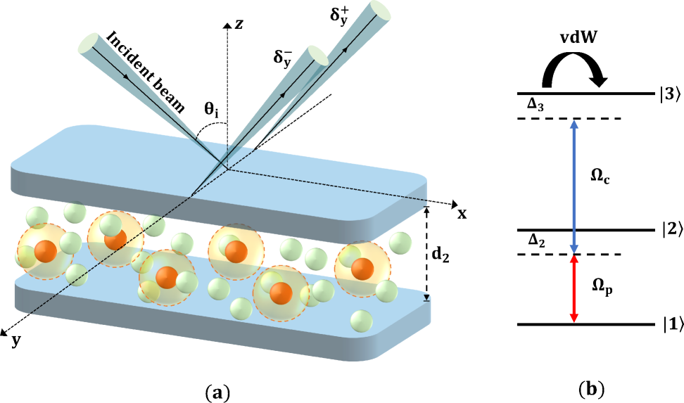
Figure 1: (a) Schematic of a three layer system with two glass slab sandwich a Rydberg atomic gas medium with susceptibility $\chi_{2}$. (b) Energy level diagram of a three-level ladder-type Rydberg EIT scheme.

The photonic spin Hall effect (PSHE) is the phenomenon in which the left and right circular polarization components of a light beam acquire opposite geometric phases upon reflection or refraction at an interface, leading to equal-magnitude, opposite-sign transverse shifts. This arises from the spin-orbit interaction of light, which converts spin-dependent phase gradients into nanometer-scale lateral displacements orthogonal to the plane of incidence. In Fig. 1(a) we consider a probe beam that is incident on the cavity from vacuum at an angel $\theta_{i}$. The cavity is consistd of two parallel semi-infinite glass slabs with susceptibility $\chi_{1}$ sandwich a homogeneous Rydberg atomic layer of thickness $d_{2}$ whose complex susceptibility is denoted as $\chi_{2}$. Inside the atomic layer, individual Rydberg excitations (red dots) are enveloped by dipole‑blockade spheres (orange dashed circles), within which further excitations are inhibited; unexcited ground‑state atoms are shown as green dots. These correlated Rydberg excitations gives rise to a strongly nonlocal nonlinear third order optical response superimposed on the usual linear susceptibility of the medium. Thus leads to a large tunability of the magnitude of PSHE in our system.

In Fig. 1(a), the $z$ axis is normal to the intersurfaces of the layered structure and $xOz$ surface is the incident plane. We denote subscript $a=i,r$ for incident and reflected beams and superscript $H$ and $V$ to mark the horizontal and vertical polarizations to the incident plane. The incident beams is considered as a parallel polarized monochromatic Gaussian beam for its simplicity, the electric field amplitude of such a beam can be written as

$$E^{H}_{i}(x_{i},y_{i})=E_{0}exp(-\frac{x_{i}^{2}+y_{i}^{2}}{\omega^{2}_{0}}),$$ (1)

where $E_{0}$ is the electric field amplitude of probe beam and $\omega_{0}$ is the beam waist. To model beam propagation and compute the PSHE quantitatively, we decompose the incident field $E^{H}_{i}(x_{i},y_{i})$ into its angular spectrum

$$\tilde{E}^{H}_{i}(k_{i}x,k_{i}y)=\int dx_{i}dy_{i}E^{H}_{i}(x_{i},y_{i})exp[-i(k_{ix}x+k_{iy}y)],$$ (2)

Each plane-wave component $\tilde{E}^{H}_{i}(k_{ix},k_{iy})$ is then treated independently. From boundary condition $k_{rx}=-k_{ix}$ and $k_{ry}=k_{iy}$, the angular spectrum of reflected beam can be obtained as[19]

$$\left[\begin{array}[]{c}\tilde{E}_{r}^{H}\\ \tilde{E}_{r}^{V}\end{array}\right]=\left[\begin{array}[]{cc}r_{p}&\frac{k_{ry}\left(r_{p}+r_{s}\right)\cot\theta_{i}}{k_{0}}\\ -\frac{k_{ry}\left(r_{p}+r_{s}\right)\cot\theta_{i}}{k_{0}}&r_{s}\end{array}\right]\left[\begin{array}[]{c}\tilde{E}_{i}^{H}\\ \tilde{E}_{i}^{V}\end{array}\right],$$ (3)

where $r_{p}$ and $r_{s}$ are the Fresnel reflection coefficients of the horizontal and vertical polarization components and $k_{0}=2\pi/\lambda_{p}$ is the central wave number of incident probe beam in vacuum.

Next, we calculate the Fresnel coefficients via a standard transfer matrix method[20]. The transfer matrix of the $j$-th layer is represented by a $2\times 2$ matrix

$$M_{j}=\left(\begin{array}[]{cc}\cos\delta_{j}&-i\frac{\sin\delta_{j}}{p_{j}}\\ -ip_{j}\sin\delta_{j}&\cos\delta_{j}\end{array}\right),$$ (4)

Here $\delta_{j}=k_{0}n_{j}d_{j}\cos\theta_{j}$ is the optical phase thickness of the $j$-th layer, and $p_{j}$ is dependent on the polarization of incident beam as $p_{j}^{p}=\frac{n_{j}}{cos[\theta_{j}]}$ and $p_{j}^{s}={n_{j}}{cos[\theta_{j}]}$. Overall, the total transfer matrix is $M=\prod_{j}M_{j}$. Denoting the incident side impedance $p_{0}=p_{1}$ and exit side $p_{N}=p_{3}$, we have the Fresnel coefficients with elements of transfer matrix $M$

$$r=\frac{\left(M_{11}+M_{12}p_{3}\right)p_{1}-\left(M_{21}+M_{22}p_{3}\right)}{\left(M_{11}+M_{12}p_{3}\right)p_{1}+\left(M_{21}+M_{22}p_{3}\right)},$$ (5)

$$t=\frac{2p_{1}}{\left(M_{11}+M_{12}p_{3}\right)p_{1}+\left(M_{21}+M_{22}p_{3}\right)},$$

Substitute Eq. (5) into Eq. (3), then write angular spectrum components in spin basis as $\tilde{E}_{r}^{\pm}=\left(\tilde{E}_{r}^{H}\mp i\tilde{E}_{r}^{V}\right)/\sqrt{2}$. Here, we must remind that the Fresnel coefficients can be expanded as a polynomial of $k_{ix}$, but we can obtain a sufficiently good approximation by confining the taylor series to the zeroth order[19].

By taking an inverse Fourier transformation of $\tilde{E}_{r}^{\pm}$, we can obtain the amplitude of reflected field. The transverse shift for the left$(\sigma=+1)$ and right$(\sigma=-1)$ circular polarized components of reflected beam can be calculated by

$$\delta_{y}^{\sigma}=\frac{\iint y_{r}\left|E_{r}^{\sigma}\left(x_{r},y_{r}\right)\right|^{2}dx_{r}dy_{r}}{\iint\left|E_{r}^{\sigma}\left(x_{r},y_{r}\right)\right|^{2}dx_{r}dy_{r}},$$ (6)

As we can clearly see that the PSHE shift $\delta_{y}^{\sigma}$ strongly depend on the incident angle $\theta_{i}$ and the susceptibility of each layer, especially the susceptibility of Rydberg atomic medium $\chi_{2}$ in our case.

In a conventional three-level Rydberg atomic system, the probe susceptibility is $\chi=\chi^{(1)}+\chi_{local}^{(3)}\left\lvert E_{p}\right\rvert^{2}$, in which has two contributions: the linear term $\chi^{(1)}$ and the local Kerr term $\chi_{local}^{(3)}$. The linear term can create the transparency window but respond weakly to other experimental knobs but the coupling field. The second term $\chi_{local}^{(3)}\varpropto N_{a}$ only adds a nonlinear correction scales linearly with atomic density $N_{a}$ which only leads to limited modulation of the total susceptibility. By contrast, a Rydberg system with many-body interaction adds a nonlocal third‐order term $\chi_{nonlocal}^{(3)}$ that scales as the square of the atomic density and extends over the blockade radius. Because the blockade radius and interaction strength depend on the Rydberg energy level, probe and coupling Rabi frequency, and atomic density, the nonlocal nonlinearity is highly versatile and can be dynamically tuned in situ. This feature gives interacting Rydberg Medium a decisive advantage in tailoring refractive and absorptive properties, enabling giant and tunable PSHE shifts that are unattainable in conventional three‐level schemes.

We consider a three‐level ladder‐type EIT scheme in the Rydberg medium (Fig. 1(b)), in which a weak probe of frequency $\omega_{p}$ drives the $|1\rangle\!\leftrightarrow\!|2\rangle$ transition at resonant frequency $\omega_{21}=\omega_{2}-\omega_{1}$, while a strong coupling field of frequency $\omega_{c}$ addresses the $|2\rangle\!\leftrightarrow\!|3\rangle$ transition at resonant frequency $\omega_{32}=\omega_{3}-\omega_{2}$. The single‐photon detunings are defined as $\Delta_{2}=\omega_{p}-\omega_{21}$, and the two‐photon detuning is $\Delta_{3}=\Delta_{2}+\Delta_{c}=\omega_{p}+\omega_{c}-(\omega_{3}-\omega_{1})$. Spontaneous emission decay from state $|\beta\rangle$ to $|\alpha\rangle$ occurs at rate $\Gamma_{\beta\alpha}$, with the corresponding coherence decay rate $\gamma_{\beta\alpha}=\Gamma_{\beta\alpha}/2\$. The nonlocal van der Waals interaction between Rydberg atoms in state $|3\rangle$ is displayed as a arc-shaped arrow above state $|3\rangle$. The vdW interaction potential is $V(r_{ij})=-C_{6}/r_{ij}^{6}$, as a function of $r_{ij}=|\mathbf{r_{i}}-\mathbf{r_{j}}|$ to describe the interaction strength between two Rydberg atoms at $\mathbf{r_{i}}$ and$\mathbf{r_{j}}$.

With above discussions, under dipole and rotating-wave approximations, the total Hamiltonian describes a three-level ladder-type Rydberg atomic system with vdW interaction is given by $\hat{H}=N_{a}\int d^{3}\mathbf{r}\mathcal{H(\mathbf{r})}$, where $N_{a}$ is the atomic density and $\mathcal{H(\mathbf{r})}$ is the Hamiltonian density given by[10]

$$\hat{\mathcal{H}}(\mathbf{r})/\hbar= -\Delta_{2}\hat{\sigma}_{22}(\mathbf{r})-\Delta_{3}\hat{\sigma}_{33}(\mathbf{r})$$ (7)

$$-\left(\Omega_{p}\hat{\sigma}_{12}(\mathbf{r})+\Omega_{c}\hat{\sigma}_{23}(\mathbf{r})+\text{ H.c. }\right)$$

$$+N_{a}\int d^{3}\mathbf{r}^{\prime}\hat{\sigma}_{33}\left(\mathbf{r}^{\prime}\right)V\left(\mathbf{r}^{\prime}-\mathbf{r}\right)\hat{\sigma}_{33}(\mathbf{r}).$$

Here, $\hat{\sigma}_{\alpha\beta}(\mathbf{r})=\lvert\beta(\mathbf{r})\rangle\langle\alpha(\mathbf{r})\rvert$ denotes the transition operator for $\alpha\neq\beta$ (and the projection operator for $\alpha=\beta$); the Rabi frequencies of the probe and coupling fields are defined by $\Omega_{p}=\mathbf{p}_{21}\cdot\mathbf{E}_{p}/(\hbar)$ and $\Omega_{c}=\mathbf{p}_{32}\cdot\mathbf{E}_{c}/(\hbar)$, respectively, where $\mathbf{p}_{21}$ and $\mathbf{p}_{32}$ are the corresponding dipole matrix elements; and the final term represents the Rydberg-Rydberg interaction, described by the van der Waals potential $V(\mathbf{r}^{\prime}-\mathbf{r})=C_{6}/|\mathbf{r}^{\prime}-\mathbf{r}|^{6}$ between atoms at $\mathbf{r}$ and $\mathbf{r}^{\prime}$. The integral term accounts for the energy shift of an atom in state $\lvert 3\rangle$ at position $\mathbf{r}$ induced by its nonlocal van der Waals interaction with an atom at position $\mathbf{r}^{\prime}$.

Applying the Heisenberg equation of motion $i\hbar\,\partial_{t}\hat{\sigma}_{\alpha\beta}(\mathbf{r})=[\hat{\sigma}_{\alpha\beta}(\mathbf{r}),\hat{\mathcal{H}}(\mathbf{r})]$, one obtains the following coupled equations for the one‐body correlators:

$$-i\tfrac{\partial}{\partial t}\rho_{11}=-i\Gamma_{12}\rho_{22}-\Omega_{p}\rho_{12}+\Omega_{p}^{*}\rho_{21},$$ (8a)

$$-i\tfrac{\partial}{\partial t}\rho_{22}=-i\Gamma_{23}\rho_{33}+i\Gamma_{12}\rho_{22}+\Omega_{p}\rho_{12}-\Omega_{p}^{*}\rho_{21}$$

$$\qquad\qquad-\Omega_{c}\rho_{23}+\Omega_{c}^{*}\rho_{32},$$ (8b)

$$-i\tfrac{\partial}{\partial t}\rho_{33}=+i\Gamma_{23}\rho_{33}+\Omega_{c}\rho_{23}-\Omega_{c}^{*}\rho_{32},$$ (8c)

$$-i\tfrac{\partial}{\partial t}\rho_{21}=-d_{21}\rho_{21}-\Omega_{p}(\rho_{22}-\rho_{11})+\Omega_{c}^{*}\rho_{31},$$ (8d)

$$-i\tfrac{\partial}{\partial t}\rho_{31}=-d_{31}\rho_{31}-\Omega_{p}\rho_{32}+\Omega_{c}\rho_{21}$$

$$\qquad\qquad-N_{a}\!\int d^{3}r^{\prime}\,V(\mathbf{r}^{\prime}-\mathbf{r})\,\rho\rho_{33,31}(\mathbf{r}^{\prime},\mathbf{r}),$$ (8e)

$$-i\tfrac{\partial}{\partial t}\rho_{32}=-d_{32}\rho_{32}-\Omega_{p}^{*}\rho_{31}-\Omega_{c}(\rho_{33}-\rho_{22})$$

$$\qquad\qquad-N_{a}\!\int d^{3}r^{\prime}\,V(\mathbf{r}^{\prime}-\mathbf{r})\,\rho\rho_{33,32}(\mathbf{r}^{\prime},\mathbf{r}).$$ (8f)

where $\rho_{\alpha\beta}(\mathbf{r},t)=\langle\hat{\sigma}_{\alpha\beta}(\mathbf{r},t)\rangle$ is the one-body density matrix element, $d_{\alpha\beta}=\Delta_{\alpha}-\Delta_{\beta}+i\gamma_{\alpha\beta}$($\Delta_{1}=0,\alpha\neq\beta$) and $\rho\rho_{\alpha\beta,\mu\nu}(\mathbf{r^{\prime}},\mathbf{r})=\langle\hat{\sigma}_{\alpha\beta}(\mathbf{r^{\prime}})\hat{\sigma}_{\mu\nu}(\mathbf{r})\rangle$ represents the quantum correlation contributed from Rydberg-Rydberg interaction.

To extract the probe susceptibility $\chi$ and its higher‐order contributions, we first relate it to the atomic coherence via $\chi=\frac{N_{a}|\mathbf{p}_{21}|^{2}}{\varepsilon_{0}\hbar}\frac{\rho_{21}}{\Omega_{p}}$; obtaining an explicit form for $\rho_{21}$ requires solving the coupled Bloch equations Eq. (8)(a)-(f), which involve two‐body correlators such as $\rho\rho_{33,31}(\mathbf{r}^{\prime},\mathbf{r})$, whose Heisenberg equation of motion can be attained via $\partial_{t}\langle\hat{\sigma}_{\alpha\beta}(\mathbf{r}^{\prime})\hat{\sigma}_{\mu\nu}(\mathbf{r})\rangle=\langle\partial_{t}\hat{\sigma}_{\alpha\beta}(\mathbf{r}^{\prime})\hat{\sigma}_{\mu\nu}(\mathbf{r})\rangle+\langle\hat{\sigma}_{\alpha\beta}(\mathbf{r}^{\prime})\partial_{t}\hat{\sigma}_{\mu\nu}(\mathbf{r})\rangle$

$$-i\tfrac{\partial}{\partial t}\rho\rho_{33,31}(\mathbf{r^{\prime}},\mathbf{r})=$$ (9)

$$\quad\left(d_{31}+i\Gamma_{23}-V\left(\mathbf{r}^{\prime}-\mathbf{r}\right)\right)\rho\rho_{33,31}(\mathbf{r^{\prime}},\mathbf{r})$$

$$\quad+\Omega_{c}\left(\rho\rho_{23,31}(\mathbf{r^{\prime}},\mathbf{r})+\rho\rho_{33,21}(\mathbf{r^{\prime}},\mathbf{r})\right)$$

$$\quad-\Omega_{c}^{*}\rho\rho_{32,31}(\mathbf{r^{\prime}},\mathbf{r})-\Omega_{p}\rho\rho_{33,32}(\mathbf{r^{\prime}},\mathbf{r})$$

$$\quad-N_{a}\int d^{3}\mathbf{r}^{\prime\prime}\left\langle\hat{\sigma}_{33}\left(\mathbf{r}^{\prime\prime}\right)\hat{\sigma}_{33}\left(\mathbf{r}^{\prime}\right)\hat{\sigma}_{31}(\mathbf{r})\right\rangle V\left(\mathbf{r}^{\prime\prime}-\mathbf{r}\right).$$

It is therefore expected that Eq. (9) involves three‐body correlators (e.g. $\left\langle\hat{\sigma}_{33}\left(\mathbf{r}^{\prime\prime}\right)\hat{\sigma}_{33}\left(\mathbf{r}^{\prime}\right)\hat{\sigma}_{31}(\mathbf{r})\right\rangle=\rho\rho\rho_{33,33,31}(\mathbf{r}^{\prime\prime},\mathbf{r}^{\prime},\mathbf{r})$) as well as additional two‐body terms such as $\rho\rho_{23,31}(\mathbf{r}^{\prime},\mathbf{r})$, leading to an infinite hierarchy of coupled equations for one‐body, two‐body, three‐body and so on. One way to close the system of equations for the correlators is to expand the correlators in the powers of the probe Rabi frequency $\Omega_{p}$[21]. This perturbation method has been detailed discussed in Ref. [10, 22]. We then apply their method by making the following expansions: $\rho_{\alpha 1}=\sum_{j=0}\Omega_{p}^{2j+1}\rho_{\alpha 1}^{(2j+1)},\rho_{\alpha\beta}=\sum_{j=1}\Omega_{p}^{2j}\rho_{\alpha\beta}^{(2j)},\rho_{11}=1+\sum_{j=1}\Omega_{p}^{2j}\rho_{11}^{(2j)}$, and for two-body correlators $\rho\rho_{\alpha\beta,\mu\nu}=\sum_{j=2}\Omega_{p}^{2j}\rho\rho_{\alpha\beta,\mu\nu}^{(2j)},\rho\rho_{1\beta,\mu\nu}=\sum_{j=1}\Omega_{p}^{2j+1}\rho\rho_{1\beta,\mu\nu}^{(2j+1)},\rho\rho_{11,\mu\nu}=\sum_{j=1}\Omega_{p}^{2j}\rho\rho_{11,\mu\nu}^{(2j)}$. With initial conditions $\rho_{11}^{(0)}=1,\rho_{22}^{(0)}=\rho_{33}^{(0)}=0$. Substitute these expansions into Eq. (8) and collect the terms of same exponential of $\Omega_{p}$. We can solve Eq. (8) in the steady state $\partial_{t}\rho_{\alpha\beta}=0$:

$$\rho_{21}^{(1)}=-\frac{d_{31}}{-|\Omega_{c}|^{2}+d_{21}d_{31}},$$ (10a)

$$\rho_{21}^{(3)}=-\frac{d_{31}(\rho_{22}^{(2)}-\rho_{11}^{(2)})-\Omega_{c}^{*}\rho_{32}^{(2)}}{|\Omega_{c}|^{2}-d_{21}d_{31}}$$

$$\qquad+\frac{\Omega_{c}^{*}N_{a}}{|\Omega_{c}|^{2}-d_{21}d_{31}}\int d^{3}\mathbf{r}^{\prime}V(\mathbf{r}^{\prime}-\mathbf{r})\rho\rho^{(3)}_{33,31}(\mathbf{r}^{\prime},\mathbf{r}),$$ (10b)

here, $\rho_{22}^{(2)}$, $\rho_{11}^{(2)}$ and $\rho_{32}^{(2)}$ are second order one‐body correlators that are independent of Rydberg-Rydberg interactions and spatial position; in Eq. (10)(b), the first term on the right‐hand side yields the local third‐order susceptibility $\chi_{\rm local}^{(3)}$, whereas the second term arises from Rydberg-Rydberg interactions and hence corresponds to the nonlocal susceptibility $\chi_{\rm nonlocal}^{(3)}$. The blockade radius $R_{b}$ is defined by equating the van der Waals interaction strength $|C_{6}|/R_{b}^{6}$ to the EIT linewidth $\delta_{\rm EIT}=|\Omega_{c}|^{2}/\gamma_{12}$ [23], since that no second atom within $|\mathbf{r}^{\prime}-\mathbf{r}|<R_{b}$ can be excited to the Rydberg state $|3\rangle$ due to the large interaction‐induced level shift; accordingly, the spatial integral in the nonlocal term of Eq. (10)(b) extends from $|\mathbf{r}^{\prime}-\mathbf{r}|=R_{b}$ to $\infty$, though in practice one may truncate the upper limit at $\sim 3R_{b}$ because $V(\mathbf{r}^{\prime}-\mathbf{r})\varpropto|\mathbf{r}^{\prime}-\mathbf{r}|^{-6}$, which decays rapidly beyond the blockade radius[16].

In Appendix A we present the detailed perturbative derivation and solution for the two‐body correlator $\rho_{33,31}^{(3)}$, and to validate our model we adopt the experimental parameters of Ref. [23]—interpreted via the Rydberg superatom framework of Ref. [24], which demonstrated that increasing the probe Rabi frequency $\Omega_{p}$ leads to a reduction in peak EIT transmission; our results in Fig. 2 reproduce this behavior and further show that the nonlocal nonlinear susceptibility $\chi_{\rm nonlocal}^{(3)}$ substantially alters both Re$[\chi^{(1)}]$ and Im$[\chi^{(1)}]$. We choose a laser-cooled ⁸⁷Rb atomic gas with atomic states $\lvert 1\rangle\equiv\lvert 5S_{1/2},F=2,m_{F}=2\rangle$, $\lvert 2\rangle\equiv\lvert 5P_{3/2},F=3,m_{F}=3\rangle$, $\lvert 3\rangle\equiv\lvert 60S_{1/2}\rangle$, with spontaneous decay rates $\Gamma_{21}=2\pi\times 6\,$MHz, $\Gamma_{32}=2\pi\times 3\,$kHz, and the corresponding van der Waals coefficient $C_{6}=2\pi\times 140\,$GHz $\cdot\mu$m⁶.

In Fig. 2 we plot the susceptibilities and transmission versus the single‐photon detuning $\Delta_{2}$ for increasing probe Rabi frequencies $\Omega_{p}/2\pi=0.01,\;0.15,\;0.5,\;1.0,\;2.0\,$MHz (top to bottom), where the red dashed (blue solid) curves denote Im$[\chi]$ (Re$[\chi]$); columns 1-3 display the linear susceptibility $\chi^{(1)}$, the local Kerr nonlinearity $\chi_{\rm local}^{(3)}$, and the nonlocal Kerr nonlinearity $\chi_{\rm nonlocal}^{(3)}$, column 4 shows the total susceptibility $\chi_{total}=\chi^{(1)}+\chi_{\rm local}^{(3)}\lvert E_{p}\rvert^{2}+\chi_{\rm nonlocal}^{(3)}\lvert E_{p}\rvert^{2}$, and column 5 gives the transmission $T=exp(-\frac{\omega_{p}L}{c}\text{Im}[\chi])$, where $L$ is the medium Length. As shown in column 5, increasing the probe Rabi frequency $\Omega_{p}$ causes, on average, more than one photon to occupy each Rydberg-blockaded atom, whereupon the strong van der Waals shifts detune additional photons out of the three-level EIT window, forcing them into a two-level–like absorption pathway and dramatically reducing the probe transmission. Comparison of columns 1-3 in Fig. 2 shows that the nonlocal third order susceptibility greatly exceeds the linear term, since it grows with $|\Omega_{p}|^{2}$ while $\chi^{(1)}$ does not depend on the probe Rabi frequency, and it outstrips the local third order term by several orders of magnitude because $\chi^{(3)}_{\rm nonlocal}\propto N_{a}^{2}$ whereas $\chi^{(3)}_{\rm local}\propto N_{a}$.

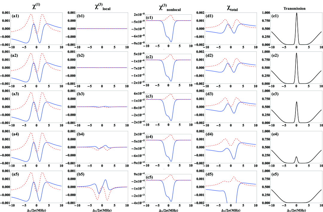
Figure 2: From first row to the last row we change $\Omega_{p}/2\pi=0.01,0.15,0.5,1.0,2.0$ MHz and plot susceptibility as a function of single photon detuning $\Delta_{2}$, the red dashed lines are the imaginary parts as the blue solid lines for real parts. The first column is Linear susceptibility $\chi^{(1)}$, second column is local nonlinear susceptibility $\chi_{local}^{(3)}$ and the third column is nonlocal nonlinear susceptibility $\chi_{nonlocal}^{(3)}$. The fourth column is the total susceptibility $\chi_{total}=\chi^{(1)}+\chi_{local}^{(3)}|E_{p}|^{2}+\chi_{nonlocal}^{(3)}|E_{p}|^{2}$ and the last column is the Transmission. Other parameters used in the calculation are $\Omega_{c}/2\pi=2.25$ MHz, the control field detuning $\Delta_{c}=\Delta_{3}-\Delta_{2}=-0.1\times 2\pi$ MHz, the atomic density $N_{a}=1.32\times 10^{7}$mm^-3 and medium length $L=1.3$mm.

III Results

In this section, we investigate the PSHE under the condition that the coupling field is detuned by $\Delta_{c}/2\pi=-0.1\,$MHz while the probe detuning $\Delta_{2}$ is varied; this configuration preserves EIT transparency at resonance and suppresses undue probe absorption. We use experimentally realistic parameters chosen to match existing Rydberg EIT experiments, and we analyze the spin dependent transverse shifts using the angular spectrum and transfer matrix methods to clarify the mechanisms behind the enhanced tunable PSHE in our proposed system. We also compare the medium susceptibility with and without Rydberg-Rydberg interactions and examine the resulting PSHE under both scenarios, in order to clearly demonstrate the impact of our scheme on enhancing and controlling the PSHE.

In Fig. 3 we present the probe susceptibility of the ladder‐type three‐level Rydberg medium, contrasting the cases with and without Rydberg-Rydberg interactions. In Fig. 3(a), the inclusion of interactions induces a pronounced nonlocal Kerr contribution, deepening and shifting the dispersive features of $\text{Re}[\chi]$. In Fig. 3(b), the interaction enhance and broaden the absorption peaks in $\text{Im}[\chi]$, while preserving the transparency window at single photon resonance. One may also sees that at the single‐photon resonance point $\Delta_{2}=0$, the imaginary part $\text{Im}[\chi]$ vanishes in the non‐interacting EIT medium but acquires a small positive offset when Rydberg-Rydberg interactions are included; this residual absorption at resonance directly produces a discernible reduction in the transmission peak, demonstrating how even a slight enhancement of $\text{Im}[\chi]$ by the nonlocal Kerr term leads to lowered on‐resonance transparency as we have demonstrated in Fig. 2.

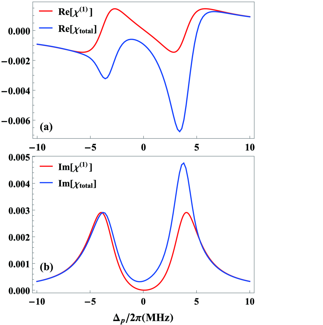
Figure 3: (a) Real part of the susceptibility $\text{Re}[\chi]$ versus probe detuning $\Delta_{2}$: the red solid curve shows the conventional three‐level ladder system without Rydberg-Rydberg interactions, and the blue solid curve includes Rydberg-Rydberg interactions. (b) Imaginary part $\text{Im}[\chi]$ under the same conditions. Other parameters used in calculation: $\Omega_{c}/2\pi=4.0\,$MHz, $\Omega_{p}/2\pi=1.0\,$MHz, $N_{a}=4\times 10^{7}\,$mm^-3, $\lambda_{p}=780\,$nm.

Fig. 4 shows the Fresnel reflection ($R_{s}$, $R_{p}$) and transmission ($T_{s}$, $T_{p}$) coefficients as functions of the incidence angle $\theta_{i}$ at probe detuning $\Delta_{2}=0$ in the glass-Rydberg-glass sandwich (glass refractive index $n\approx 1.49$, Rydberg‐layer thickness $d_{2}=1\,$mm). At normal incidence, both $R_{s}$ and $R_{p}$ start near the theoretical value $[(n_{2}-1)/(n_{2}+1)]^{2}\approx 4\%$, modulated by millimeter‐scale interference fringes; $R_{p}$ then falls to zero at the Brewster angle $\theta_{B}\approx\arctan(n_{2})\approx 33.8^{\circ}$ while $R_{s}$ rises monotonically toward unity, and the corresponding transmissions $T_{s}$ and $T_{p}$ decrease from their maxima at $\theta_{i}=0$ to zero as $\theta_{i}\to 42.2^{\circ}$, in agreement with energy conservation and the onset of total reflection.

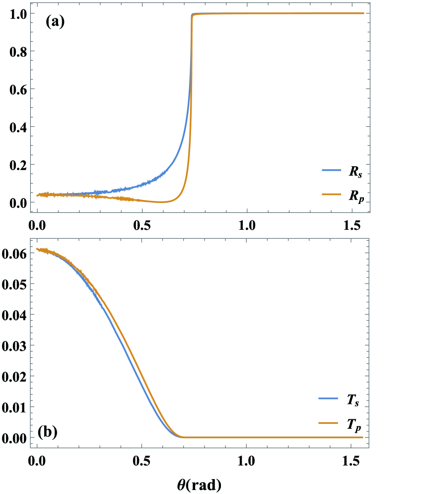
Figure 4: (a) Fresnel reflection ($R_{s}$, $R_{p}$) and (b) transmission ($T_{s}$, $T_{p}$) coefficients versus incidence angle $\theta_{i}$ for s‐ (blue) and p‐polarization (orange) at zero probe detuning ($\Delta_{2}=0$).

To demonstrate the contribution of Rydberg-Rydberg interactions, we present the PSHE computed with the nonlocal Kerr term disabled ($\chi_{\rm nonlocal}^{(3)}=0$) as a reference. In Fig 5, we present the spin‐dependent transverse shifts $\delta_{y}^{+}$(Fig 5(a)) and $\delta_{y}^{-}$(Fig 5(b)) for left‐ and right‐circular polarizations, respectively, as functions of probe detuning $\Delta_{2}$ and incidence angle $\theta_{i}$ with Gaussian waist $\omega_{0}=50\,\mu$m, showing the expected symmetric sign inversion of equal‐magnitude shifts in a narrow band around the Brewster angle ($33.8^{\circ}$); superimposed on this ideal PSHE ridge are detuning‐dependent, wave‐like ripples as slight oscillations in the red‐blue boundary, which reflects the Kerr susceptibility modulation induced by the atomic layer with change of probe detuning $\Delta_{2}$. Next, we analyze the PSHE as a function of probe detuning $\Delta_{2}$ with incident angle $\theta_{i}=33.87^{\circ}$ as shown by blue line in Fig. 6(a), at a fixed incident angle near the Brewster condition, the PSHE shift $\delta_{y}^{+}$ varies with probe detuning $\Delta_{2}$, exhibiting positive and negative peaks at $\Delta_{2}/2\pi\thickapprox 3\text{MHz}$ and crossing zero at resonance ($\Delta_{2}=0$); this behavior reflects the strong modulation of the reflection phase slope by the atomic medium’s Kerr susceptibilities, enabling detuning‐controlled reversible switching of the spin‐dependent displacement and enhancement of the PSHE. However, in Fig. 6(b) we repeat the detuning scan at a slightly different incidence angle, $\theta_{i}=33.84^{\circ}$ (blue solid line), keeping all other parameters fixed. The resulting $\delta_{y}^{+}(\Delta_{2})$ reproduces the same overall trend—rising to a positive peak near $\Delta_{2}/2\pi\approx 3\text{MHz}$ and falling through zero to a negative trough near $-3\text{MHz}$—but the extrema now occur at unequal magnitudes and the positive lobe fails to reach its theoretical maximum. This comparison highlights the extreme sensitivity of the PSHE to sub‐degree angular alignment: even a $0.03^{\circ}$ shift in $\theta_{i}$ alters both the peak amplitude and the balance between positive and negative displacements. As we can see, in the absence of Rydberg atom interactions, the atomic medium still modulates the PSHE shift as probe detuning varies, but in a conventional three‐level EIT scheme the susceptibility is independent of the probe Rabi frequency, so scanning $\Delta_{2}$ alone cannot amplify the response sufficiently to produce both maximal positive and maximal negative displacements; at best it yields a single unidirectional extremum, revealing the fundamental limitations of such ladder‐type configurations for PSHE enhancement.

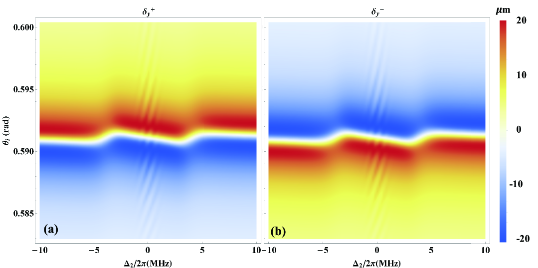
Figure 5: (a) Density plot of PSHE shift $\delta_{y}^{+}$ and (b) $\delta_{y}^{-}$ versus incident angle $\theta_{i}$ and probe detuning $\Delta_{2}$ without Rydberg-Rydberg interaction. Other parameters are the same in Fig. 3.

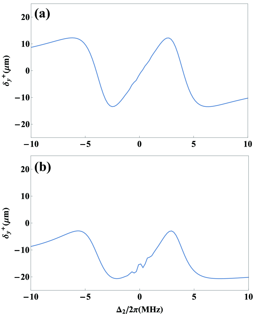
Figure 6: The PSHE shift $\delta_{y}^{+}$ versus probe dutuning $\Delta_{2}$ at incident angle (a) $\theta_{i}=33.87^{\circ}$ and (b) $\theta_{i}=33.84^{\circ}$ without Rydberg-Rydberg interaction. Other parameters are the same in Fig. 3.

By way of comparison with the non‐interacting reference, in Fig. 7, we plot the PSHE shifts for the left‐ (panel a) and right‐circular (panel b) polarization components as functions of probe detuning $\Delta_{2}$ and incidence angle $\theta_{i}$ in the presence of Rydberg-Rydberg interactions, revealing how the nonlocal Kerr nonlinearity reshapes the shift amplitude contours of the PSHE ridge near the Brewster angle. In contrast to the nearly uniform, symmetric ridge observed without Rydberg interactions (Fig. 5), the interacting medium exhibits pronounced undulations and asymmetric broadening of the positive‐ and negative‐shift contours in Fig. 7, indicating that the nonlocal Kerr response not only amplifies the overall PSHE amplitude but also introduces detuning‐ and angle‐dependent phase‐slope perturbations that break the ideal mirror symmetry and sharpen the shift’s sensitivity to both $\Delta_{2}$ and $\theta_{i}\,$. In Fig. 8 shows the PSHE shift $\delta_{y}^{+}$ as a function of probe detuning $\Delta_{2}$ at fixed incidence angle $\theta_{i}=33.85^{\circ}$ with Rydberg-Rydberg interactions enabled, revealing two full‐amplitude extrema of opposite sign—approximately $\pm 20\mu$m—centered near $\Delta_{2}/2\pi\approx 3\text{MHz}$. This demonstrates that the nonlocal Kerr nonlinearity allows the system to reach both maximal positive and maximal negative displacements by detuning alone, overcoming the intrinsic limitations of the non‐interacting ladder scheme.

Fig. 9 complements Fig. 8 by mapping the normalized transverse intensity profiles of the reflected beam at two representative detunings. At $\Delta_{2}/2\pi=3$MHz the left-circular component peaks at $y=+20\mu\text{m}$ while the right-circular component peaks at $y=-20\mu\text{m}$; changing the detuning to $6$MHz reverses these positions, directly visualizing the detuning-controlled sign flip of the PSHE shift.

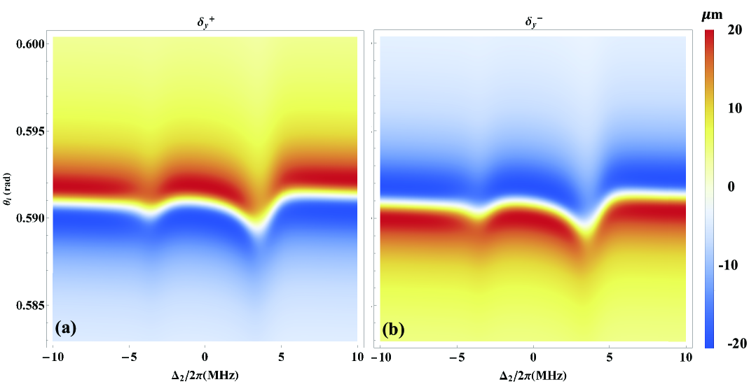
Figure 7: (a) Density plot of PSHE shift $\delta_{y}^{+}$ and (b) $\delta_{y}^{-}$ versus incident angle $\theta_{i}$ and probe detuning $\Delta_{2}$ with Rydberg-Rydberg interaction. Other parameters are the same in Fig. 3.

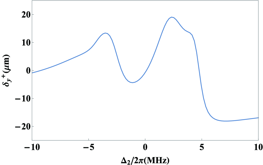
Figure 8: The PSHE shift $\delta_{y}^{+}$ versus probe dutuning $\Delta_{2}$ at incident angle $\theta_{i}=33.85^{\circ}$ with Rydberg-Rydberg interaction. Other parameters are the same in Fig. 3.

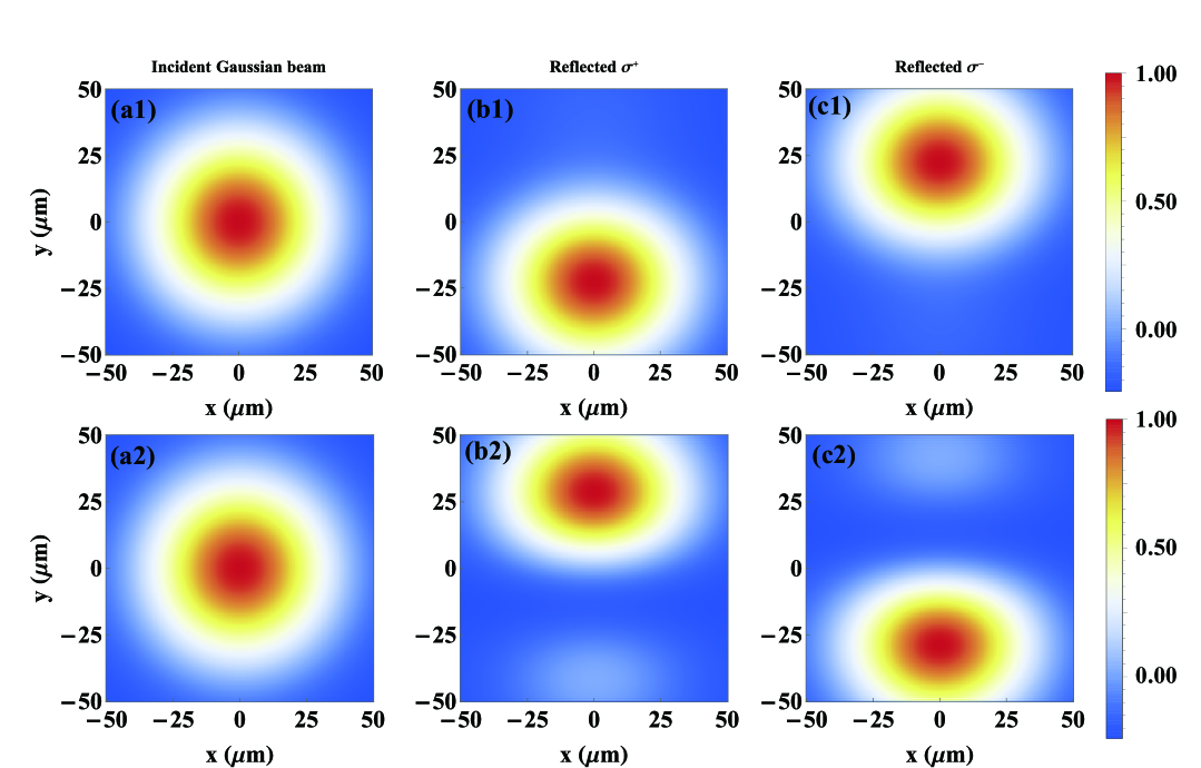
Figure 9: The distribution of normalized transverse intensity for (a)incident Gaussian beam (b) reflected left-cicular polarized field and (c) reflected right-cicular polarized field. The first row corresponds to probe detuning $\Delta_{2}/2\pi=3$MHz and the second row corresponds to probe detuning $\Delta_{2}/2\pi=6$MHz. Other parameters are the same in Fig. 3.

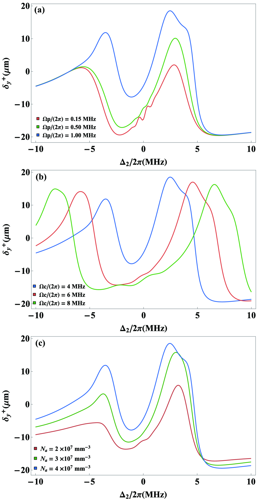
Figure 10: (a) The PSHE shift $\delta_{y}^{+}$ versus probe dutuning $\Delta_{2}$ at incident angle $\theta_{i}=33.85^{\circ}$ with Rydberg-Rydberg interaction for $\Omega_{p}/2\pi=0.15$ MHz (orange line), $0.50$ MHz (green line), $1.00$ MHz (blue line). (b) The PSHE shift $\delta_{y}^{+}$ versus probe dutuning $\Delta_{2}$ at incident angle $\theta_{i}=33.85^{\circ}$ with Rydberg-Rydberg interaction for $\Omega_{c}/2\pi=4$ MHz (blue line), $6$ MHz (orange line), $8$ MHz (green line). (c) The PSHE shift $\delta_{y}^{+}$ versus probe dutuning $\Delta_{2}$ at incident angle $\theta_{i}=33.85^{\circ}$ with Rydberg-Rydberg interaction for $N_{a}=2\times 10^{7}\text{mm}^{-3}$ (orange line), $3\times 10^{7}\text{mm}^{-3}$ (green line), $4\times 10^{7}\text{mm}^{-3}$ MHz (blue line). Other parameters are the same in Fig. 3.

In Fig. 10 we show the detuning dependence of the PSHE shift $\delta_{y}^{+}$ under variation of (a) the probe Rabi frequency $\Omega_{p}$, (b) the coupling Rabi frequency $\Omega_{c}$, and (c) the atomic density $N_{a}$, with all other parameters held as in Fig. 3. Fig. 10(a) illustrates how $\delta_{y}^{+}$ responds to an increasing probe Rabi frequency, when the probe is weak ($\Omega_{p}/2\pi=0.15\text{MHz}$), only a small fraction of atoms is excited to Rydberg state, resulting the Rydberg-Rydberg interaction is therefore negligible, the medium susceptibility differs little from its linear EIT value as the orange curve of Fig. 10(a) is similar to Fig. 6(b). Increasing the probe strength to $\Omega_{p}/2\pi=0.5\text{MHz}$ populates more atoms into Rydberg state thus enhances the van der Waals interaction and correspondingly the nonlocal nonlinear susceptibility $\chi_{nonlocal}^{(3)}\varpropto N_{a}^{2}|\Omega_{p}|^{2}$, leads to a positive lobe around $\Delta_{2}/2\pi\approx 3\text{MHz}$. Therefore, at highest drive $\Omega_{p}/2\pi=1.00\text{MHz}$, the interaction induced index dominates the dispersion, yielding nearly symmetric positive and negative extrema in Fig. 8. Fig. 10(b) shows that increasing $\Omega_{c}$ broadens EIT transparency window consequently, the dispersion inflection points and hence the extrema of $\delta_{y}^{+}$ shift outward along the detuning axis. Notably the peak magnitude of shift remains nearly constant, confirming that the coupling field primarily tunes the operational detuning range without altering the nonlocal Kerr contribution generated by the Rydberg-Rydberg interaction. Finally, in Fig. 10(c), we examine the influence of atomic density by varying $N_{a}=2,3,4\times 10^{7}\text{mm}^{-3}$, same as the effect in Fig. 10(a), as $\chi_{nonlocal}^{(3)}\varpropto N_{a}^{2}|\Omega_{p}|^{2}$, a higher $N_{a}$ will strengthen the van der Waals interaction and amplifies the modulation experienced by the probe.

Building on these results, Rydberg-Rydberg interactions offers clear benefits over a standard three-level medium. The nonlocal Kerr term scales with the square of the atomic density and extends across the blockade radius, yielding a nonlinear susceptibility that can exceed the linear term by orders of magnitude even at moderate densities and thereby enhancing PSHE shifts without high optical power. Because the blockade radius, interaction strength and susceptibility profile all depend on the chosen Rydberg state and on the probe and coupling Rabi frequencies, tuning these parameters enables real-time control of the PSHE, unlike fixed-response ladder EIT schemes. Extended interactions also introduce detuning and angle dependence in the reflection phase slope, breaking the mirror symmetry of the PSHE ridge and allowing positive and negative extrema to be reached separately. These enhancements persist over wide detuning and incidence-angle ranges, providing a robust platform for ultrahigh‐sensitivity displacement and refractive‐index sensing that passive atomic media cannot match.

IV Conclusions

In summary, we have presented a comprehensive study of the photonic spin Hall effect in a glass-Rydberg-glass sandwich cavity driven under a ladder‐type EIT scheme. We expanded the Bloch equations up to third order in the probe field and incorporated both the ordinary Kerr response and the interaction-driven nonlocal Kerr term into a multilayer transfer matrix approach. We demonstrated that Rydberg-Rydberg interactions strongly reshape the medium’s susceptibility. This enhanced nonlocal nonlinearity not only amplifies the spin‐dependent transverse shifts, but also breaks the strict dependence on incidence-angle tuning: at a fixed angle near Brewster’s condition, both positive and negative PSHE extrema can now be accessed simply by scanning the probe detuning. These findings suggest a clear path toward PSHE-based photonic devices, by leveraging frequency tuning rather than mechanical alignment, such platforms could achieve rapid, reconfigurable metrology and signal processing in future photonic devices.

Appendix A APPENDIX: DERIVATION OF PERTURBATION METHOD

In addition to Eq. (9), other dynamic equations of two-body correlators are

$$\left(i\frac{\partial}{\partial t}+d_{23}+d_{31}\right)\rho\rho_{23,31}+\Omega_{c}\rho\rho_{23,21}+\Omega_{p}(\rho\rho_{13,31}-\rho\rho_{23,32})-N_{a}\int d^{3}\mathbf{r}^{\prime\prime}\left\langle\hat{\sigma}_{33}\left(\mathbf{r}^{\prime\prime}\right)\hat{\sigma}_{23}\left(\mathbf{r}^{\prime}\right)\hat{\sigma}_{31}(\mathbf{r})\right\rangle V\left(\mathbf{r}^{\prime\prime}-\mathbf{r}\right)=0.$$ (11a)

$$\left(i\frac{\partial}{\partial t}+d_{32}+d_{31}-V\left(\mathbf{r}^{\prime}-\mathbf{r}\right)\right)\rho\rho_{32,31}+\Omega_{c}(\rho\rho_{22,31}+\rho\rho_{32,21})-\Omega_{p}(\rho\rho_{31,31}-\rho\rho_{32,32})$$

$$-N_{a}\int d^{3}\mathbf{r}^{\prime\prime}\left\langle\hat{\sigma}_{33}\left(\mathbf{r}^{\prime\prime}\right)\hat{\sigma}_{32}\left(\mathbf{r}^{\prime}\right)\hat{\sigma}_{31}(\mathbf{r})\right\rangle V\left(\mathbf{r}^{\prime\prime}-\mathbf{r}\right)=0.$$ (11b)

$$\left(i\frac{\partial}{\partial t}+d_{21}+i\Gamma_{23}\right)\rho\rho_{33,21}+\Omega_{c}\rho\rho_{23,21}+\Omega_{p}(\rho\rho_{33,11}-\rho\rho_{33,22})+\Omega_{c}^{*}\left(\rho\rho_{33,31}-\rho\rho_{32,21}\right)=0.$$ (11c)

$$\left(i\frac{\partial}{\partial t}+d_{31}+i\Gamma_{12}\right)\rho\rho_{22,31}+\Omega_{c}(\rho\rho_{22,21}-\rho\rho_{23,31})+\Omega_{p}(\rho\rho_{12,31}-\rho\rho_{21,31}-\rho\rho_{22,32})+\Omega_{c}^{*}\rho\rho_{32,31}$$

$$-N_{a}\int d^{3}\mathbf{r}^{\prime\prime}\left\langle\hat{\sigma}_{33}\left(\mathbf{r}^{\prime\prime}\right)\hat{\sigma}_{22}\left(\mathbf{r}^{\prime}\right)\hat{\sigma}_{31}(\mathbf{r})\right\rangle V\left(\mathbf{r}^{\prime\prime}-\mathbf{r}\right)=0.$$ (11d)

$$\left(i\frac{\partial}{\partial t}+d_{21}+d_{23}\right)\rho\rho_{23,21}+\Omega_{p}(\rho\rho_{13,21}-\rho\rho_{23,11}-\rho\rho_{23,22})+\Omega_{c}^{*}(\rho\rho_{23,31}+\rho\rho_{33,21}-\rho\rho_{22,21})=0.$$

$$-N_{a}\int d^{3}\mathbf{r}^{\prime\prime}\left\langle\hat{\sigma}_{33}\left(\mathbf{r}^{\prime\prime}\right)\hat{\sigma}_{23}\left(\mathbf{r}^{\prime}\right)\hat{\sigma}_{21}(\mathbf{r})\right\rangle V\left(\mathbf{r}^{\prime\prime}-\mathbf{r}\right)=0.$$ (11e)

$$\left(i\frac{\partial}{\partial t}+d_{21}+d_{32}\right)\rho\rho_{32,21}+\Omega_{c}(\rho\rho_{22,21}-\rho\rho_{33,21})+\Omega_{p}(\rho\rho_{32,11}-\rho\rho_{31,21}-\rho\rho_{32,22})+\Omega_{c}^{*}\rho\rho_{32,31}=0.$$ (11f)

$$\left(i\frac{\partial}{\partial t}+d_{21}+i\Gamma_{12}\right)\rho\rho_{22,21}-\Omega_{c}\rho\rho_{23,21}+\Omega_{p}(\rho\rho_{12,21}-\rho\rho_{21,21}-\rho\rho_{22,22}+\rho\rho_{22,11})+\Omega_{c}^{*}(\rho\rho_{22,31}+\rho\rho_{32,21})=0.$$ (11g)

These equations constitute a closed set of equations for $\rho\rho_{33,31}$, to be more specific we address that one may notice that there are the interaction terms such as $V\left(\mathbf{r}^{\prime}-\mathbf{r}\right)\rho\rho_{32,31}$ is out of the integration. This arises from the delta-function extraction property when commuting projection operators in the integral of the many-body interaction term using commutation relations

$$[\hat{\sigma}_{\alpha\beta}(\mathbf{r}),\hat{\sigma}_{\mu\nu}(\mathbf{r}^{\prime})]=(\delta_{\alpha\nu}\hat{\sigma}_{\mu\beta}(\mathbf{r})-\delta_{\mu\beta}\hat{\sigma}_{\alpha\nu}(\mathbf{r}^{\prime}))\delta_{\mathbf{rr^{\prime}}}.$$ (12)

Next, substituting the perturbation expansion and retaining the third-order terms, we obtain the following system of equations $Q\mathbf{x}^{(3)}=\mathbf{q}$:

$$Q=\left[\begin{array}[]{cccccccc}d_{31}+i\Gamma_{23}-V(\mathbf{r^{\prime}}-\mathbf{r})&\Omega_{c}&-\Omega_{c}^{*}&\Omega_{c}&0&0&0&0\\ \Omega_{c}^{*}&d_{23}+d_{31}&0&0&-\Omega_{c}^{*}&\Omega_{c}&0&0\\ -\Omega_{c}&0&d_{31}+d_{32}-V(\mathbf{r^{\prime}}-\mathbf{r})&0&\Omega_{c}&0&\Omega_{c}&0\\ \Omega_{c}^{*}&0&0&d_{21}+i\Gamma_{23}&0&\Omega_{c}&-\Omega_{c}^{*}&0\\ 0&-\Omega_{c}&\Omega_{c}^{*}&0&d_{31}+i\Gamma_{12}&0&0&\Omega_{c}\\ 0&\Omega_{c}^{*}&0&\Omega_{c}^{*}&0&d_{21}+d_{23}&0&-\Omega_{c}^{*}\\ 0&0&\Omega_{c}^{*}&-\Omega_{c}&0&0&d_{21}+d_{32}&-\Omega_{c}^{*}\\ 0&0&0&0&\Omega_{c}^{*}&-\Omega_{c}&\Omega_{c}^{*}&d_{21}+i\Gamma_{12}\end{array}\right]$$ (13)

$$\mathbf{x}^{(3)}=\left[\rho\rho_{33,31}^{(3)},\rho\rho_{23,31}^{(3)},\rho\rho_{32,31}^{(3)},\rho\rho_{33,21}^{(3)},\rho\rho_{22,31}^{(3)},\rho\rho_{23,21}^{(3)},\rho\rho_{32,21}^{(3)},\rho\rho_{22,21}^{(3)}\right]^{T},$$ (14)

$$\mathbf{q}=\left[\begin{array}[]{c}0\\ -\rho\rho_{12,31}^{(2)}\\ \rho\rho_{31,31}^{(2)}\\ -\rho_{33}^{(2)}\\ -\rho\rho_{12,31}^{(2)}+\rho\rho_{21,31}^{(2)}\\ -\rho_{23}^{(2)}+\rho\rho_{13,21}^{(2)}\\ -\rho_{32}^{(2)}+\rho\rho_{31,21}^{(2)}\\ -\rho_{22}^{(2)}-\rho\rho_{12,21}^{(2)}+\rho\rho_{21,21}^{(2)}\end{array}\right],$$ (15)

And for second order terms in $\mathbf{q}$, we follow the previous procedure, write dynamic equations of two-body correlators then retain the second-order terms,

$${\left[\begin{array}[]{cccc}d_{13}+d_{31}&-\Omega_{c}^{*}&0&\Omega_{c}\\ -\Omega_{c}&d_{12}+d_{31}&\Omega_{c}&0\\ 0&\Omega_{c}^{*}&d_{12}+d_{21}&-\Omega_{c}\\ \Omega_{c}^{*}&0&-\Omega_{c}^{*}&d_{13}+d_{21}\end{array}\right]\left[\begin{array}[]{l}\rho\rho_{13,31}^{(2)}\\ \rho\rho_{12,31}^{(2)}\\ \rho\rho_{12,21}^{(2)}\\ \rho\rho_{13,21}^{(2)}\end{array}\right]}$$ (16)

$$=\left[\begin{array}[]{c}0\\ \rho_{31}^{(1)}\\ -\rho_{12}^{(1)}+\rho_{21}^{(1)}\\ -\rho_{13}^{(1)}\end{array}\right],$$

$${\left[\begin{array}[]{cccc}2d_{31}-V(\mathbf{r}^{\prime}-\mathbf{r})&2\Omega_{c}&0&0\\ \Omega_{c}^{*}&d_{21}+d_{31}&\Omega_{c}&0\\ 0&0&2d_{21}&2\Omega_{c}^{*}\\ \Omega_{c}^{*}&0&\Omega_{c}&d_{21}+d_{31}\end{array}\right]\left[\begin{array}[]{l}\rho\rho_{31,31}^{(2)}\\ \rho\rho_{21,31}^{(2)}\\ \rho\rho_{21,21}^{(2)}\\ \rho\rho_{31,21}^{(2)}\end{array}\right]}$$ (17)

$$=\left[\begin{array}[]{c}0\\ \rho_{31}^{(1)}\\ -2\rho_{21}^{(1)}\\ -\rho_{31}^{(1)}\end{array}\right],$$

References

- Bliokh and Aiello [2013] K. Y. Bliokh and A. Aiello, Journal of Optics 15, 014001 (2013).
- Bliokh et al. [2008] K. Y. Bliokh, A. Niv, V. Kleiner, and E. Hasman, Nature Photonics 2, 748 (2008).
- Hosten and Kwiat [2008] O. Hosten and P. Kwiat, Science 319, 787 (2008).
- Luo et al. [2011a] H. Luo, X. Zhou, W. Shu, S. Wen, and D. Fan, Physical Review A—Atomic, Molecular, and Optical Physics 84, 043806 (2011a).
- Chen et al. [2020] S. Chen, X. Ling, W. Shu, H. Luo, and S. Wen, Physical review applied 13, 014057 (2020).
- Ling et al. [2015] X. Ling, X. Zhou, X. Yi, W. Shu, Y. Liu, S. Chen, H. Luo, S. Wen, and D. Fan, Light: Science & Applications 4, e290 (2015).
- Yin et al. [2013] X. Yin, Z. Ye, J. Rho, Y. Wang, and X. Zhang, Science 339, 1405 (2013).
- Zahra et al. [2025] N. Zahra, Y. Mizutani, T. Uenohara, and Y. Takaya, Scientific Reports 15, 12911 (2025).
- Bardon-Brun et al. [2019] T. Bardon-Brun, D. Delande, and N. Cherroret, Physical review letters 123, 043901 (2019).
- Bai and Huang [2016] Z. Bai and G. Huang, Optics express 24, 4442 (2016).
- Sinclair et al. [2019] J. Sinclair, D. Angulo, N. Lupu-Gladstein, K. Bonsma-Fisher, and A. M. Steinberg, Physical Review Research 1, 033193 (2019).
- Busche et al. [2017] H. Busche, P. Huillery, S. W. Ball, T. Ilieva, M. P. Jones, and C. S. Adams, Nature Physics 13, 655 (2017).
- Gorniaczyk et al. [2016] H. Gorniaczyk, C. Tresp, P. Bienias, A. Paris-Mandoki, W. Li, I. Mirgorodskiy, H. Büchler, I. Lesanovsky, and S. Hofferberth, Nature communications 7, 12480 (2016).
- Baur et al. [2014] S. Baur, D. Tiarks, G. Rempe, and S. Dürr, Physical review letters 112, 073901 (2014).
- Xu et al. [2020] H. Xu, C. Hang, and G. Huang, Physical Review A 101, 053832 (2020).
- Zheng et al. [2022] D.-D. Zheng, H.-M. Zhao, X.-J. Zhang, and J.-H. Wu, Physical Review A 106, 043119 (2022).
- Abbas et al. [2025] M. Abbas, P. Zhang, and H. R. Hamedi, Physical Review A 111, 043708 (2025).
- Waseem et al. [2024] M. Waseem, M. Shah, and G. Xianlong, Physical Review A 110, 033104 (2024).
- Luo et al. [2011b] H. Luo, X. Ling, X. Zhou, W. Shu, S. Wen, and D. Fan, Physical Review A—Atomic, Molecular, and Optical Physics 84, 033801 (2011b).
- Wu et al. [2010] L. Wu, H.-S. Chu, W. S. Koh, and E.-P. Li, Optics express 18, 14395 (2010).
- Sevinçli et al. [2011] S. Sevinçli, N. Henkel, C. Ates, and T. Pohl, Physical review letters 107, 153001 (2011).
- Zhang et al. [2018] Q. Zhang, Z. Bai, and G. Huang, Physical Review A 97, 043821 (2018).
- Pritchard et al. [2010] J. D. Pritchard, D. Maxwell, A. Gauguet, K. J. Weatherill, M. Jones, and C. S. Adams, Physical review letters 105, 193603 (2010).
- Petrosyan et al. [2011] D. Petrosyan, J. Otterbach, and M. Fleischhauer, Physical review letters 107, 213601 (2011).