Convergence rates of regularized quasi-Newton methods without strong convexity

Abstract

In this paper, we study convergence rates of the cubic regularized proximal quasi-Newton method (Cubic SR1) for solving non-smooth additive composite problems that satisfy the so-called Kurdyka-Łojasiewicz (KŁ) property with respect to some desingularization function $\varphi$ rather than strong convexity. After a number of iterations $k_{0}$, Cubic SR1  exhibits non-asymptotic explicit super-linear convergence rates for any $k\geq k_{0}$. In particular, when $\varphi(t)=ct^{1/2}$, Cubic SR1 PQN has a convergence rate of order $\left(\frac{C}{(k-k_{0})^{1/2}}\right)^{(k-k_{0})/2}$, where $k$ is the number of iterations and $C>0$ is a constant. For the special case, i.e. functions which satisfy Łojasiewicz inequality, the rate becomes global and non-asymptotic. This work presents, for the first time, non-asymptotic explicit convergence rates of regularized (proximal) SR1 quasi-Newton methods applied to non-convex non-smooth problems with KŁ  property. Actually, the rates are novel even in the smooth non-convex case. Notably, we achieve this without employing line search or trust region strategies, without assuming the Dennis-Moré condition, without any assumptions on quasi-Newton metrics and without assuming strong convexity. Furthermore, for convex problems, we focus on a more tractable gradient regularized quasi-Newton method (Gradient SR1) which can achieve results similar to those obtained with cubic regularization. We also demonstrate, for the first time, the non-asymptotic super-linear convergence rate of Gradient SR1for solving convex problems with the help of the Łojasiewicz inequality instead of strong convexity.

1 Introduction

Quasi-Newton methods have been studied extensively over decades due to their fast convergence. They have been developed to approximate the Hessian (second derivative) of the objective [18], using solely first-order information. Based on this idea, numerous variants have been developed, including BFGS [11], SR1 [16, 10], DFP [16, 22]. A striking advantage of quasi-Newton-type methods [11, 12, 19, 21, 24, 13] for minimizing some strongly convex smooth function $f$ is the local super-linear convergence. However, the convergence rates obtained by these works above are asymptotic, i.e., $\lim_{k\to\infty}\frac{\|x_{k+1}-x^{*}\|}{\|x_{k}-x^{*}\|}\to 0$ or $\lim_{k\to\infty}\frac{\|\nabla f(x_{k+1})\|}{\|\nabla f(x_{k})\|}\to 0$. Since an asymptotic statement is about the limit as $k\to\infty$, we are also interested in a non-asymptotical analysis where the convergence rate is valid for any $k$ or at least for all $k\geq k_{0}$ where $k_{0}$ is some constant. Only a non-asymptotic statement can characterize an explicit upper bound on the error of quasi Newton methods. Recently, on strongly convex problems, many outstanding results [45, 46, 28, 52] provide non-asymptotic explicit local super-linear convergence rates for classical quasi-Newton schemes including BFGS and SR1. However, the guarantee is their local convergence, meaning that the initial point must be close to the minimum point. To study global rates, [44, 27] adopt BFGS with line-search strategies, while [51] studies SR1 method on a composite problem with solely regularization strategy.

In this paper, we would like to generalize the results from [51] to problems without strong convexity. A possible way is to assume the objective function $f$ has the Kurdyka-Łojasiewicz (KŁ) property [6, 8, 35, 42], which can be regarded as a generalization of strong convexity. Based on the KŁ inequality with a special concave function $\varphi(t)=ct^{1-\theta}$ where $\theta\in(0,1)$, the convergence rates of first-order methods on convex or non-convex problems have been developed [53, 35, 23]. If $\varphi$ is unique for any point $x\in\mathrm{dom}\,F$, it leads to the gradient-dominated functions studied by Polyak and Nesterov in [39, 31]. In this paper, we give non-asymptotic convergence rates by studying cubic- and gradient-regularized quasi-Newton methods from [51] with the help of the KŁ  property. This paper consists of two parts. In the first part, we provide convergence analysis of cubic regularized PQN on non-convex non-smooth problems under general $\varphi$ or $\varphi=ct^{1-\theta}$ of different $\theta\in(0,1)$. In particular, when $\theta\in(0,\frac{1}{2})$, we show an explicit super-linear convergence rate $O(\frac{C}{N^{1/2}})^{N/2}$ for some $C$ after a certain number of iterations. In the second part, we specialize on the convex case and use more tractable gradient regularization, rather than cubic regularization, to achieve similar results. The main contribution of this paper is to reveal that KŁ inequality is the key property for the fast convergence of quasi-Newton methods. It is also worth emphasizing that we do not assume the Dennis-Moré condition in this paper which is, in fact, the characteristic of super-linear convergence and widely assumed by many papers [15, 48, 13]. Furthermore, we have no assumptions on our quasi-Newton metrics. We also do not adopt any line search or trust region strategies to achieve global convergence.

2 Related Works

Regularized Newton method.

Despite global convergence on convex problem can be obtained while maintaining the local fast convergence [17, 40] by using line search or trust region stategies, there are other regularization strategies to achieve the same goal by adding a positive definite matrix to the Hessian (like in the Levenberg–Marquardt method [34, 37]). Thanks to having a positive definite metric, Newton’s methods are stabilized at the cost of loosing the local fast convergence rates. The pioneering work by Nesterov and Polyak [39] has introduced cubic regularization as another globalization strategy that avoids line search and at the same time shows the standard fast local convergence rates of the pure Newton’s method. This cubic regularization works even on non-convex problems such as star-convex function or gradient dominated functions, namely, one satisfying the condition that for any $x\in\mathrm{dom}\,f$, $f(x)-{\color[rgb]{0,0,0}f^{*}}\leq C\|\nabla f(x)\|^{p}$ with some $C>0$, $p>0$. In order to remedy the computational cost of cubic regularization, in [38, 20] a gradient regularization strategy was introduced for solving convex problems. It also allows for global convergence with a super-linear rate of convergence for strongly convex problems. Motivated by their works, [51] proposed two regularized SR1 proximal quasi Newton methods with non-asymptotic super-linear convergence rate on strongly convex problems These works have fundamentally inspired the present paper. We will further study the non-asymptotic convergence rates of two algorithms from [51] without assuming strong convexity.

Quasi-Newton methods.

Rodomanov and Nesterov [45] obtained the first local explicit super-linear convergence rate for greedy quasi-Newton methods. Later, Haishan Ye et al [52] obtained the first local explicit super-linear convergence rate for the SR1 quasi-Newton method, introducing several fruitful techniques about SR1 scheme. Building on this, [51] studies the global rates. Both works significantly inspired our development in this paper. However, all results above require the strong convexity of the objective function. Therefore, it is worth looking for non-asymptotic super-linear convergence rates of quasi Newton methods on convex or even non-convex problems. In our paper, we study regularized (cubic, gradient) proximal SR1 methods from [51], showing non-asymptotic super-linear rates without the help of strong convexity.

There are a few more works, appearing under similar names like ‘regularized Newton-type method’ [14, 30, 4, 5, 36, 25]. Since they do not consider non-asymptotic convergence rates and are using line search or trust region strategies, we do not describe them in more detail here. As for cubic regularization, in the well-known work [13], they considered asymptotic convergence of quasi-Newton method on non-convex smooth problem via assuming the Dennis-Moré condition. There is another way to develop an cubic regularized inexact Newton method without the explicit computation of Hessian via using finite difference [26]. Cubic regularization quasi Newton method is also studied in [29] on star-convex problems. However, the super-linear performance of quasi Newton methods is not investigated in [29].

Proximal quasi-Newton and Newton-type methods.

One of the earliest work on proximal quasi-Newton methods is [15], where they adopted line search to guarantee global convergence and assume the Dennis–Moré criterion to obtain asymptotic super-linear convergence. [33] also demonstrated an asymptotic super-linear local convergence rate of the proximal Newton and a proximal quasi-Newton method under the same condition. Both papers are based on convex problems. We believe that the Dennis–Moré criterion is very restrictive and hard to check. We assume Lipschitz continuity of the Hessian and KŁ property instead. Later, [47] showed that by a prox-parameter update mechanism, rather than a line search, they can derive a sub-linear global complexity on convex problems. However, to the best of our knowledge, there is no result on non-asymptotic explicit super-linear convergence rates for a proximal quasi-Newton method on composite problems without strong convexity. While we focus on the convergence rate, the efficient evaluation of proximal mapping with respect to variable metric is also crucial. There are a few works [47, 32, 2] that are associated to this topic. In particular, [2] proposed a proximal calculus to tackle this difficulty, followed by [3, 50, 30].

3 Preliminaries

3.1 Notation

We first introduce our notation. We denote $\overline{\mathbb{R}}=\mathbb{R}\cup{\{+\infty\}}$ and $\mathbb{R}_{+}=[0,\infty)$. $\mathbb{R}^{n}$ is an Euclidean vector space of dimension $n$, which is equipped with the standard Euclidean norm $\|u\|:=\sqrt{u^{\top}u}$, for any $u\in\mathbb{R}^{n}$. Given symmetric positive definite $M\in\mathbb{R}^{n\times n}$, we denote $\|u\|_{M}=\sqrt{u^{\top}Mu}$. Given a matrix $A\in\mathbb{R}^{n\times n}$, $\|A\|$ denotes the matrix norm induced by the Euclidean vector norm. We write $\mathrm{tr}\,A$ for the trace of the matrix $A\in\mathbb{R}^{n\times n}$. Moreover, $I$ denotes the identity matrix in $\mathbb{R}^{n}$. We adopt the standard definition of the Loewner partial order of symmetric positive semi-definite matrices. Let $A$ and $B$ be two symmetric positive semi-definite matrices, we say $A\preceq B$ (or $A\prec B$) if and only if for any $u\in\mathbb{R}^{n}$, we have $u^{\top}(B-A)u\geq 0$ (or $u^{\top}(B-A)u>0$, respectively). Let $F\colon\mathbb{R}^{n}\to\mathbb{R}$ be a function. The domain of $F$ is defined as $\mathrm{dom}F=\{x|F(x)<+\infty\}$. For any $\alpha,\beta\in(0,\infty]$ with $\alpha<\beta$, we denote the set $\{x|\alpha<F(x)<\beta\}$ by $[\alpha<F(x)<\beta]$. Let $(x_{k})_{k\in\mathbb{N}}$ be a sequence in $\mathbb{R}^{n}$ starting from $x_{0}$. The set of all limit points of $(x_{k})_{k\in\mathbb{N}}$ is denoted by $\omega(x_{0})$, i.e.,

$$\omega(x_{0})=\{x\in\mathbb{R}^{n}|\text{$\exists\,(x_{k_{q}})_{q\in\mathbb{N}}$ such that $x_{k_{q}}\to x$ as $q\to\infty$}\}\,.$$

We denote $[N,k]\coloneqq\{i\in\mathbb{N}|k\leq i\leq N+k\}$ for any $N,k\in\mathbb{N}$.

3.2 Subdifferentials of non-convex and non-smooth functions

Definition 3.1 (Subdifferentials).

Let $F\colon\mathbb{R}^{n}\to\overline{\mathbb{R}}$ be a proper and lower semi-continuous function.

1. For a given $x\in\mathrm{dom}\,F$, the Fréchet subdifferential of $F$ at $x$, written $\hat{\partial}F(x)$, is the set of all vectors $u\in\mathbb{R}^{n}$ which satisfy

   $$\liminf_{y\neq x\ y\to x}\frac{F(y)-F(x)-\left\langle u,y-x\right\rangle}{\|y-x\|}\geq 0\,.$$

   For $x\notin\mathrm{dom}\,F$, we set $\hat{\partial}F(x)=\emptyset$.

2. The limiting-subdifferential [43] or simply the subdifferential, of $F$ at $x\in\mathrm{dom}\,F$, written $\partial F(x)$, is defined through the following closure process

   $$\partial F(x)\coloneqq\{u\in\mathbb{R}^{n}:\exists\ x_{k}\to x,\ F(x_{k})\to F(x)\ \text{and}\ u_{k}\to u\ \text{where $u_{k}\in\hat{\partial}F(x_{k})$}\ \text{as $k\to\infty$}\}\,.$$

We denote $\mathrm{crit}F\coloneqq\{x|\partial F(x)\ni 0\}$. We recall the definition of Kurdyka-Łojasiewicz property from [1].

Definition 3.2 (Kurdyka-Łojasiewicz).

Let $\eta\in(0,+\infty]$. We denote by $\Phi_{\eta}$ the class of concave functions $\varphi\colon[0,\eta)\to\mathbb{R}_{+}$ which satisfy the following conditions: $\varphi\colon[0,\eta)\to\mathbb{R}_{+}$ is continuous; $\varphi(0)=0$; $\varphi$ is continuously differentiable on $(0,\eta)$ with $\varphi^{\prime}(s)>0$, for any $s\in(0,\eta)$.

Now we define the Kurdyka-Łojasiewicz (KŁ) property. A proper, lower semi-continuous function $F$ is said to have Kurdyka-Lojasiewicz (KŁ) property at $\bar{x}\in\mathrm{dom}\partial F$ if there exist $\eta\in(0,+\infty]$, a neighborhood $U$ of $\bar{x}$ and a continuous concave function $\varphi\in\Phi_{\eta}$ such that the Kurdyka-Lojasiewicz inequality holds, i.e.,

$$\varphi^{\prime}\left(F(x)-F(\bar{x})\right)\mathrm{dist}\left(0,\partial F(x)\right)\geq 1\,,$$ (1)

for all $x$ in $U\cap[F(\bar{x})<F(x)<F(\bar{x})+\eta]$. If $F$ satisfies the KŁ inequality at any $x\in\mathrm{dom}\partial F$, then $F$ is called a KŁ function.

All tame (definable) functions are KŁ functions [7]. In particular, for any $\bar{x}$, semi-algebraic functions have the KŁ property at any $\bar{x}$ with $\varphi$ of the form $\varphi(t)=ct^{1-\theta}$ for some $c\in\mathbb{R}_{+}$ and $\theta\in(0,1]$ [1]. Computing the KŁ exponent $\theta$ is hard but crucial. We refer readers to [35] for the calculus of KŁ exponent. Since the KŁ inequality of KŁ function is valid locally, we need a uniformized KŁ property [9].

Lemma 3.1 (Uniformized KŁ property [9]).

Let $\Omega$ be a compact set and let $F\colon\mathbb{R}^{n}\to(-\infty,+\infty]$ be a proper and lower semi-continuous function. Assume $F$ is constant on $\Omega$ and satisfies the KŁ  property at each point of $\Omega$. Then, there exists $\epsilon>0$, $\eta>0$ and $\varphi\in\Phi_{\eta}$ such that for all $\bar{x}\in\Omega$ and all $x$ in the following intersection

$$\{x\in\mathbb{R}^{n}|\mathrm{dist}(x,\Omega)<\epsilon\}\cap[F(\bar{x})<F(x)<F(\bar{x})+\eta]\,,$$ (2)

one has

$$\varphi^{\prime}\left(F(x)-F(\bar{x})\right)\mathrm{dist}\left(0,\partial F(x)\right)\geq 1\,.$$ (3)

4 Problem Setup and Main Results

In this section, we present the considered problem setup with all standing assumptions and our main results. We postpone the technical parts of the convergence analysis to Section 5.

4.1 Problem set up

In the whole paper, we consider the optimization problem:

$$\min_{x\in\mathbb{R}^{n}}F(x)\,,\quad\text{where}\ F(x)\coloneqq g(x)+f(x)\,,$$ (4)

where we make the following assumptions:

Assumption 1.

1. $F=g+f$ is bounded from below and coercive;

2. $g\colon\mathbb{R}^{n}\to\overline{\mathbb{R}}$ is proper, lower semi-continuous (lsc), (possibly non-convex);

3. $f\colon\mathbb{R}^{n}\to\mathbb{R}$ is twice differentiable with $L$-Lipschitz gradient, $L_{H}$-Lipschitz Hessian (possibly non-convex).

Assumption 2.

$F$ is a KŁ function.

4.2 Algorithms and main results

Let us first recap the classical symmetric rank-1 quasi-Newton (SR1) update $G_{+}\coloneqq\text{SR1}(A,G,u)$. Given two $n\times n$ symmetric matrices $A$ and $G$ such that $A\preceq G$ and $u\in\mathbb{R}^{n}$, we define the SR1 update as follows:

$$\text{SR1}(A,G,u):=\begin{cases}G\,,&\ \text{if}\ (G-A)u=0\,;\\ G-\frac{(G-A)uu^{\top}(G-A)}{u^{\top}(G-A)u}\,,&\ \text{otherwise}\,.\end{cases}$$ (5)

In order to solve the problem in (4), we study a cubic regularized proximal SR1 quasi-Newton method (Algorithm 1). Algorithm 1 (Cubic SR1) is similar with the first algorithm proposed in [51]. The only difference is that we will apply the same algorithm with a restarting strategy on non-convex problem. Step 1 has two cases. If $\mathrm{tr}\,G_{k}\leq n\bar{\kappa}$, Step 1a is executed. Otherwise, Step 1b implements a special proximal gradient update step with cubic regularization. Step 2 defines $J_{k}$ which is not used explicitly. Step 4 updates the quasi Newton metric via SR1 method.

We obtain global convergence with the following local explicit rates.

Algorithm 1 Cubic SR1

$x_{0}$, $G_{0}=LI$, $r_{-1}=0$, $\bar{\kappa}\geq L$ .

Update for $k=0,\cdots,N$:

1. 1. If $\mathrm{tr}\,G_{k}\leq n\bar{\kappa}$: update

      $$x_{k+1}\in\operatorname*{argmin}_{x\in\mathbb{R}^{n}}g(x)+\left\langle\nabla f(x_{k}),x-x_{k}\right\rangle+\frac{1}{2}\|x-x_{k}\|_{G_{k}+L_{H}r_{k-1}I}^{2}+\frac{L_{H}}{3}\|x-x_{k}\|^{3}\,.$$ (6)

      Compute $u_{k}=x_{k+1}-x_{k}$, $r_{k}=\|u_{k}\|$, $\lambda_{k}=L_{H}r_{k-1}+L_{H}r_{k}$.

      Compute $\tilde{G}_{k+1}=G_{k}+\lambda_{k}I$ (Correction step).

   2. Otherwise: compute

      $$x_{k+1}=\operatorname*{argmin}_{x\in\mathbb{R}^{n}}g(x)+\left\langle\nabla f(x_{k}),x-x_{k}\right\rangle+\frac{L+L_{H}r_{k-1}}{2}\|x-x_{k}\|^{2}+\frac{L_{H}}{3}\|x-x_{k}\|^{3}\,.$$ (7)

      Compute $u_{k}=x_{k+1}-x_{k}$, $r_{k}=\|u_{k}\|$, $\lambda_{k}=L_{H}r_{k-1}+L_{H}r_{k}$.

      Compute $\tilde{G}_{k+1}=LI+\lambda_{k}I$ (Restart step)

2. Denote but do not use explicitly $J_{k}\coloneqq\int_{0}^{1}\nabla^{2}f(x_{k}+tu_{k})dt$ .

3. Compute

   $$\begin{split}F^{\prime}(x_{k+1})=&\ \nabla f(x_{k+1})-\nabla f(x_{k})-{\tilde{G}_{k+1}}u_{k}\,.\\ \end{split}$$

4. Update quasi-Newton metric:

   $$G_{k+1}=\text{SR1}(J_{k},{\tilde{G}_{k+1}},u_{k})\,.$$

5. If $\|F^{\prime}(x_{k+1})\|=0$: Terminate.

End

Theorem 4.1.

Let Assumption 1 and 2 hold. Cubic SR1 PQN (Algorithm 1) has $\|F^{\prime}(x_{N})\|\to 0$, $F(x_{N})\to F^{*}$ for some $F^{*}\in\mathbb{R}$ and $\mathrm{dist}(x_{N},\mathrm{crit}F)\to 0$ as $N\to\infty$. Moreover, there exists $k_{0}\in\mathbb{N}$ such that for any $k\geq k_{0}$, Cubic SR1 PQN (Algorithm 1) has a local convergence rate:

$$\left(\min_{i\in[N,k_{0}]}\|F^{\prime}(x_{i})\|\right)\leq\left(C_{1}\left(\frac{C_{\mathrm{CR1}}}{N}+\frac{C_{\mathrm{CR2}}}{N^{1/2}}\right)\right)^{N/(N+1)}\|F^{\prime}(x_{k_{0}})\|^{2/(N+1)}\,;$$ (8)

where $N=k-k_{0}$, $[N,k_{0}]\coloneqq\{i\in\mathbb{N}|k_{0}\leq i\leq N+k_{0}\}$, $C_{\mathrm{CR1}}\coloneqq{\color[rgb]{0,0,0}nL+n\bar{\kappa}+2nL_{H}d}$, $C_{\mathrm{CR2}}\coloneqq{\color[rgb]{0,0,0}2nL_{H}C_{0}}$, $C_{0}\coloneqq\sqrt{\frac{3r_{k_{0}}^{2}}{2}+M(\varphi(F(x_{k_{0}})-{\color[rgb]{0,0,0}F^{*}}))}$, $M\coloneqq\frac{3D}{L_{H}}$, $D=(2n\bar{\kappa}+2L+2L_{H}d)$, $C_{1}\coloneqq 3\varphi(F(x_{k_{0}})-{\color[rgb]{0,0,0}F^{*}})$ and $d$ is the diameter of $\{x|F(x)\leq F(x_{0})\}$.
Furthermore, for the case that $\varphi$ has the form $\varphi(t)=ct^{1-\theta}$ for some $c>0$, Cubic SR1 PQN has better convergence rates:

1. If $\theta\in(0,\frac{1}{2})$, it has a superlinear convergence rate:

   $$\|F^{\prime}(x_{N+k_{0}})\|\leq\left(C\left(\frac{C_{\mathrm{CR1}}}{N}+\frac{C_{\mathrm{CR2}}}{N^{1/2}}\right)\right)^{N/2}\|F^{\prime}({\color[rgb]{0,0,0}x_{k_{0}}})\|\,;$$ (9)

2. if $\theta=\frac{1}{2}$, it has a superlinear convergence rate:

   $$\|F^{\prime}(x_{N+k_{0}})\|\leq\left(\frac{3c^{2}}{4}\left(\frac{C_{\mathrm{CR1}}}{N}+\frac{C_{\mathrm{CR2}}}{N^{1/2}}\right)\right)^{N/2}\|F^{\prime}({\color[rgb]{0,0,0}x_{k_{0}}})\|\,;$$ (10)

3. if $\theta\in(\frac{1}{2},1)$,

   $$\min_{i\in[N,k_{0}]}\|F^{\prime}(x_{i})\|\leq\left(C_{2}\left(\frac{C_{\mathrm{CR1}}}{N}+\frac{C_{\mathrm{CR2}}}{N^{1/2}}\right)\|F^{\prime}(x_{k_{0}})\|^{2/N}\right)^{N/(2+(N-1)(2-\frac{1}{\theta}))}\,,$$ (11)

   where $C_{2}=3((1-\theta)c)^{1/\theta}$ and $C=C_{1}^{\frac{1-2\theta}{1-\theta}}C_{2}^{\frac{\theta}{1-\theta}}$.

Proof.

See Section 5.2. ∎

Remark 4.2.

The convergence analysis of Theorem 4.1 relies on the uniformized KŁ property of $x$ in (2). We can obtain global convergence rates if we have $\epsilon=+\infty$ and $\eta=+\infty$ which is surprisingly satisfied by many problems. For instances, a gradient dominated differentiable $f$ with nonempty $\Omega=\arg\min f$, i.e., $f$ satisfies the following inequality:

$$f(x)-\inf f\leq\frac{c^{2}}{4}\|\nabla f(x)\|^{2}\,,$$

for any $x\in\mathrm{int}\,\mathrm{dom}\,f$ and some $c>0$ which is also called Łojasiewicz inequality. It is equivalent to say that (3) is valid for any $x\in\mathrm{dom}\,f$ with respect to $\Omega=\arg\min f$ and $\varphi(t)=ct^{1/2}$. To minimize this function $f$, for any $N\in\mathbb{N}$, Algorithm 1 exhibits a non-asymptotic superlinear convergence rate:

$$\|\nabla f(x_{N})\|\leq\left(C\left(\frac{\overline{C}_{\mathrm{CR1}}}{N}+\frac{\overline{C}_{\mathrm{CR2}}}{N^{1/2}}\right)\right)^{N/2}\|\nabla f(x_{0})\|\,.$$ (12)

where $\overline{C}_{\mathrm{CR1}}\coloneqq nL+nL+2nL_{H}d$, $\overline{C}_{\mathrm{CR2}}\coloneqq{2nL_{H}C_{0}}$, $C_{0}\coloneqq\sqrt{\frac{3r_{k_{0}}^{2}}{2}+M(\varphi(F(x_{0})-{\inf f}))}$, $M\coloneqq\frac{3D}{L_{H}}$, $D=(n\bar{\kappa}+2L+2L_{H}d)$, $C_{1}\coloneqq 3\varphi(F(x_{0})-{\inf f})$ and $d$ is the diameter of $\{x|F(x)\leq F(x_{0})\}$. In fact, if we assume $f$ satisfies Łojasiewicz inequality and $g=0$, then we can derive the following superlinear convergence rate by a simple modification of the proof of Theorem 4.1 without using restart strategy (See Appendix A):

$$\|\nabla f(x_{N})\|\leq\frac{\mu}{6}\left(\left(\frac{O}{N^{1/3}}\right)\right)^{N/2}\|\nabla f(x_{0})\|\,,$$ (13)

where $O=\left(2nL+2nL_{H}d+2nL_{H}\left(\frac{6}{L_{H}}\left(f(x_{0})-\inf f\right)\right)^{1/3}\right)$ and $d$ is the diameter of the sub-level set $\{x|f(x)\leq f(x_{0})\}$.

Remark 4.3.

In fact, in the case when $\varphi(t)=ct^{1/2}$, (10) indicates that the super-linear rate is attained after $N+k_{0}\geq\max\{C_{\mathrm{CR1}},C_{\mathrm{CR2}}^{2}\}+k_{0}$ number of iterations. Here $C_{\mathrm{{CR1}}}=O(n)$ and $C_{\mathrm{{CR2}}}=O(n^{3/2})$ where $n$ is the number of dimension. Therefore, the super-linear rate is attained after $O({\color[rgb]{0,0,0}n^{3}})+k_{0}$ iterations.

Remark 4.4.

The Łojasiewicz inequality is equivalent to the error bound condition of Hoffman’s type and to the quadratic growth rate condition, which is first established in the seminal paper by Zhang [53]. Therefore, our results can be generalized to problems with error bound conditions.

Remark 4.5.

We compare our results with convergence rates of first order methods. When $N$ is sufficiently large, for a general $\varphi$, the Cubic SR1 PQN has a sub-linear convergence rate $O\left(\frac{1}{N^{1/2}}\right)$, whereas no convergence rate is established for first order methods in this case [23]. Now, we consider the case when $\varphi=ct^{1-\theta}$. For $\theta\in(0,\frac{1}{2}]$, first order methods achieve linear convergence rates [35, 31] while our Cubic SR1 method attains a super-linear convergence rate. When $\theta\in\left(\frac{1}{2},1\right)$, the first order methods have convergence rates $O\left(\frac{1}{N^{\frac{1-\theta}{2\theta-1}}}\right)$ (see [23], whereas our Cubic SR1 method has a convergence rate close to $O\left(\frac{1}{N^{\frac{\theta}{2(2\theta-1)}}}\right)$. For $\frac{1}{2}<\theta<\frac{2}{3}$, the convergence rate of our Cubic SR1 PQN is slower than that of first order methods [23], but for $\frac{2}{3}<\theta\leq 1$ our Cubic SR1 PQN achieves a faster convergence rate.

If we additionally assume $f$ and $g$ are convex functions, then $F$ is convex and we can apply a gradient regularized quasi Newton method. That is Algorithm 2 which is the same as the third algorithm proposed in [51]. We recap the algorithm here for readers’ convenience.

Algorithm 2 Grad SR1 PQN

$x_{0}$, $G_{0}=LI$, $\lambda_{0}=0$, $\tilde{G}_{0}=G_{0}+\lambda_{0}$, $\bar{\kappa}\geq L$ .

Update for $k=0,\cdots,N$:

1. Update

   $$x_{k+1}=\operatorname*{argmin}_{x\in\mathbb{R}^{n}}g(x)+\left\langle\nabla f(x_{k}),x-x_{k}\right\rangle+\frac{1}{2}\|x-x_{k}\|_{\tilde{G}_{k}}^{2}\,.$$ (14)

2. Denote but do not use explicitly $J_{k}\coloneqq\int_{0}^{1}\nabla^{2}f(x_{k}+tu_{k})dt$ .

3. Compute $u_{k}=x_{k+1}-x_{k}$, $r_{k}=\|u_{k}\|$, and

   $$\begin{split}F^{\prime}(x_{k+1})=&\ \nabla f(x_{k+1})-\nabla f(x_{k})-\tilde{G}_{k}u_{k}\,,\\ G_{k+1}=&\ \text{SR1}(J_{k},\tilde{G}_{k},u_{k})\,,\\ \lambda_{k+1}=&\ \left(\sqrt{L_{H}\|F^{\prime}(x_{k+1})\|}+L_{H}r_{k}\right)\,.\end{split}$$

4. Update $\tilde{G}_{k+1}$: compute $\hat{G}_{k+1}=G_{k+1}+\lambda_{k+1}I$ (Correction step).

   1. If $\mathrm{tr}\,{\hat{G}_{k+1}}\leq n\bar{\kappa}$: we set $\tilde{G}_{k+1}=\hat{G}_{k+1}$ .

   2. Othewise: we set $\tilde{G}_{k+1}=LI$ (Restart step).

5. If $\|F^{\prime}(x_{k+1})\|=0$: Terminate.

End

For gradient regularized proximal quasi-Newton methods, we obtain global convergence with the following non-asymptotic rates.

Theorem 4.6.

Let Assumption 1 and 2 hold. Additionally, we assume both $g$, $f$ are convex. For any initialization $x_{0}\in\mathbb{R}^{n}$ Grad SR1 PQN (Algorithm 2) has $\|F^{\prime}(x_{N})\|\to 0$, $F(x_{k})\to\inf F$ and $\mathrm{dist}(x_{N},\mathrm{crit}F)\to 0$ as $N\to\infty$. Moreover, there exists $k_{0}\in\mathbb{N}$ such that for any $k\geq k_{0}$, Grad SR1 PQN (Algorithm 2) has a non-asymptotic rate:

$$\left(\min_{k\in[N,k_{0}]}\|F^{\prime}(x_{k})\|\right)\leq\left(S_{1}\left(\frac{n\bar{\kappa}}{N}+\frac{C_{\mathrm{GR}}}{N^{1/3}}\right)\right)^{N/(N+1)}\|F^{\prime}({x_{k_{0}}})\|^{2/(N+1)}\,;$$ (15)

where $N=k-k_{0}$, $C_{\mathrm{GR}}\coloneqq nDC_{0}^{1/3}$, $C_{0}\coloneqq\frac{r_{k_{0}}^{3/2}}{3}+\sqrt{\frac{4(n\bar{\kappa}+L)}{L_{H}}}(\varphi(F({\color[rgb]{0,0,0}x_{k_{0}}})-{\color[rgb]{0,0,0}\inf F}))$, $D\coloneqq(\sqrt{L_{H}(n\bar{\kappa}+L)}+L_{H}d)$, $d$ is the diameter of $\{x|F(x)\leq F({\color[rgb]{0,0,0}x_{k_{0}}})\}$ and $S_{1}=2\varphi(F({\color[rgb]{0,0,0}x_{k_{0}}})-{\color[rgb]{0,0,0}\inf F})$.
Furthermore, for the case $\varphi$ has the form $\varphi(t)=ct^{1-\theta}$ for some $c>0$, Grad SR1 PQN has better convergence rates:

1. if $\theta\in(0,\frac{1}{2})$, it has a super-linear convergence rate:

   $$\|F^{\prime}(x_{N+k_{0}})\|\leq\left(S\left(\frac{n\bar{\kappa}}{N}+\frac{C_{\mathrm{GR}}}{N^{1/3}}\right)\right)^{N/2}\|F^{\prime}({\color[rgb]{0,0,0}x_{k_{0}}})\|\,,$$ (16)

2. if $\theta=\frac{1}{2}$, it has a super-linear convergence rate:

   $$\|F^{\prime}(x_{N+k_{0}})\|\leq\left(\frac{c^{2}}{2}\left(\frac{n\bar{\kappa}}{N}+\frac{C_{\mathrm{GR}}}{N^{1/3}}\right)\right)^{N/2}\|F^{\prime}({\color[rgb]{0,0,0}x_{k_{0}}})\|\,,$$ (17)

3. if $\theta\in(\frac{1}{2},1)$, it has a sub-linear convergence rate:

   $$\min_{k\in[N,k_{0}]}\|F^{\prime}(x_{k})\|\leq\left(S_{2}\left(\frac{n\bar{\kappa}}{N}+\frac{C_{\mathrm{GR}}}{N^{1/3}}\right)\|F^{\prime}({\color[rgb]{0,0,0}x_{k_{0}}})\|^{2/N}\right)^{1/(\frac{2}{N}+2-\frac{1}{\theta})}\,,$$ (18)

   where $S_{2}=2(1-\theta)c^{2}$ and $S=S_{1}^{\frac{1-2\theta}{1-\theta}}S_{2}^{\frac{\theta}{1-\theta}}$.

Proof.

See Section 5.3. ∎

Remark 4.7.

The convergence analysis of Theorem 4.6 also relies on the uniformized KŁ property of $F$ with respect to $\Omega=\min F$. We can obtain global convergence rates for this algorithm if we have $\epsilon=+\infty$ and $\eta=+\infty$.

Remark 4.8.

In fact, in the case when $\varphi(t)=ct^{1/2}$, (10) indicates that the super-linear rate is attained after $N+k_{0}\geq\max\{n\bar{\kappa},C_{\mathrm{GR}}^{3}\}+k_{0}$ number of iterations and $C_{\mathrm{GR}}=O(n^{5/3})$. Therefore, the super-linear rate is attained after $O(n^{5})+k_{0}$ iterations.

Let $g=0$. Let $f$ satisfy Assumption 1 and Łojasiewicz inequality:

$$f(x)-{\color[rgb]{0,0,0}\inf f}\leq\frac{c}{2}\|\nabla f(x)\|^{2}\,,$$ (19)

for some $c>0$ and any $x\in\mathrm{int}\,\mathrm{dom}\,f$. A better global convergence rate can be retrieved.

Theorem 4.9.

Let Assumption 1 and 2 hold. Additionally, we assume $g=0$ and $f$ is a convex function satisfying (19). For any initialization $x_{0}\in\mathbb{R}^{n}$ Grad SR1 PQN (Algorithm 2) has $\|\nabla f(x_{N})\|\to 0$ as $N\to+\infty$ and Grad SR1 PQN (Algorithm 2) has a global non-asymptotic rate:

$$\|\nabla f(x_{N})\|\leq\left(\frac{c^{2}C_{\mathrm{GD}}}{2N}\right)^{N/(2)}\|\nabla f({\color[rgb]{0,0,0}x_{0}})\|^{2/(N+1)}\,;$$ (20)

where $C_{\mathrm{GD}}\coloneqq(n\bar{\kappa}+n\sqrt{L_{H}}C_{f}+nL_{H}C_{r})$, $C_{f}=4n\bar{\kappa}(cn\bar{\kappa}(f(x_{0})-{\color[rgb]{0,0,0}\inf f}))^{1/4}$ and

$$C_{r}=\frac{1}{\sqrt{L_{H}}}4cn\bar{\kappa}(2n\bar{\kappa}(f(x_{0})-{\color[rgb]{0,0,0}\inf f}))^{1/4}+\frac{1}{L}2cn\bar{\kappa}(2n\bar{\kappa}(f(x_{0})-{\color[rgb]{0,0,0}\inf f}))^{1/2}\,.$$

Proof.

See Section 5.3. ∎

Remark 4.10.

(20) indicates that the super-linear rate is attained after $N\geq C_{\mathrm{GD}}$ number of iterations and $C_{\mathrm{GD}}=O(n^{2.5})$.

5 Convergence Analysis

In this section, without loss of generality, we assume that $\|F^{\prime}(x_{k})\|>0$ for any $k\in\mathbb{N}$, since, otherwise, our algorithms terminate after a finite number of steps and our non-asymptotic rates would hold until then. And for convenience, we denote $F^{\prime}(x_{0})$ as any subgradient of $F(x)$ at $x_{0}$.

Recall that throughout the whole convergence analysis, we assume that Assumption 1 and 2 holds and that all variables are defined in Algorithm 1.

5.1 Several useful properties

First, we need several important properties of $J_{k}\coloneqq\int_{0}^{1}\nabla^{2}f(x_{k}+tu_{k})dt$, which is the same for both algorithms.

Lemma 5.1.

For each $k\in\mathbb{N}$, we have

$$f(x_{k+1})-f(x_{k})\leq\left\langle\nabla f(x_{k}),u_{k}\right\rangle+{\frac{1}{2}}\left\langle\nabla^{2}f(x_{k})u_{k},u_{k}\right\rangle+\frac{L_{H}}{6}\|u_{k}\|^{3}\,,$$ (21)

$$f(x_{k+1})-f(x_{k})\leq\left\langle\nabla f(x_{k}),u_{k}\right\rangle+{\frac{1}{2}}\left\langle J_{k}u_{k},u_{k}\right\rangle+\frac{L_{H}}{6}\|u_{k}\|^{3}\,.$$ (22)

Proof.

The first result is from [39, Lemma 1]. Using a similar argument as in [39, Lemma 1], we can derive the second result. For any $y,x\in\mathbb{R}^{n}$, we have

$$\begin{split}&\|\nabla f(y)-\nabla f(x)-\int_{0}^{1}\nabla^{2}f(x+s(y-x))(y-x)ds\|\\ &\leq\|\int_{0}^{1}\int_{0}^{1}(\nabla^{2}f(x+t(y-x))-f(x+s(y-x)))(y-x)dtds)\|\\ &\leq L_{H}\|y-x\|^{2}\int_{0}^{1}\int_{0}^{1}|t-s|dtds\\ &\leq\frac{1}{3}L_{H}\|y-x\|^{2}\,.\end{split}$$ (23)

Therefore, we have

$$\begin{split}|f(x_{k+1})-f(x_{k})-\left\langle\nabla f(x_{k}),u_{k}\right\rangle-\frac{1}{2}\left\langle J_{k}u_{k},u_{k}\right\rangle|&\leq|\int_{0}^{1}\left\langle\nabla f(x_{k}+tu_{k})-\nabla f(x_{k})-tJ_{k}u_{k},u_{k}\right\rangle dt|\\ &\leq|\int_{0}^{1}\left\langle\nabla f(x_{k}+tu_{k})-\nabla f(x_{k})-tJ_{k}u_{k},u_{k}\right\rangle dt|\\ &\leq\frac{L_{H}}{3}\|u_{k}\|^{3}\int_{0}^{1}t^{2}dt\\ &=\frac{L_{H}}{6}\|u_{k}\|^{3}\\ \end{split}$$ (24)

∎

Lemma 5.2.

For each $k\in\mathbb{N}$, we have $-LI\preceq J_{k}\preceq LI$.

Proof.

Since $f$ has $L$-Lipschitz gradient, we have $-LI\preceq\nabla^{2}f(x)\preceq LI$ for any $x\in\mathbb{R}^{n}$. Thus, due to the definition of $J_{k}$, we have $-LI\preceq J_{k}\preceq LI$. ∎

Lemma 5.3.

For each $k\in\mathbb{N}$, we have

$$J_{k}\preceq J_{k-1}+\frac{1}{2}L_{H}(r_{k}+r_{k-1})I\,,$$ (25)

$$\nabla^{2}f(x_{k})\preceq J_{k-1}+\frac{1}{2}L_{H}r_{k-1}I\,,$$ (26)

$$\nabla^{2}f(x_{k})\preceq J_{k}+\frac{1}{2}L_{H}r_{k}I\,.$$ (27)

Proof.

The proof is similar with the one of [45, Lemma 4.2], [52, Lemma 5]. The assumption that the Hessian of $f$ is $L_{H}$-Lipschitz continuous means that there exists $L_{H}>0$ such that for any $x,y\in\mathbb{R}^{n}$, we have

$$\|\nabla^{2}f(x)-\nabla^{2}f(y)\|\leq L_{H}\|x-y\|\,.$$ (28)

For any $t,s\in[0,1]$ and $k\in\mathbb{N}$, letting $x=x_{k}+tu_{k}$ and $y=x_{k}-(1-s)u_{k-1}$, we have that

$$\|\nabla^{2}f(x_{k}+tu_{k})-\nabla^{2}f(x_{k}-(1-s)u_{k})\|\leq L_{H}\|tu_{k}+(1-s)u_{k-1}\|\,.$$ (29)

Then, by the definition of $J_{k}$, we have

$$\begin{split}J_{k}-J_{k-1}&=\int_{0}^{1}\nabla^{2}f(x_{k}+tu_{k})dt-\int_{0}^{1}\nabla^{2}f(x_{k-1}+su_{k-1})ds\\ &=\int_{0}^{1}\nabla^{2}f(x_{k}+tu_{k})dt-\int_{0}^{1}\nabla^{2}f(x_{k}-(1-s)u_{k-1})ds\\ &\preceq\int_{0}^{1}\|\nabla^{2}f(x_{k}+su_{k})-\nabla^{2}f(x_{k}-(1-s)u_{k-1})\|ds\cdot I\\ &\preceq\int_{0}^{1}L_{H}\|su_{k}+(1-s)u_{k-1}\|dt\cdot I\\ &\preceq\frac{1}{2}L_{H}(r_{k}+r_{k-1})I\,,\end{split}$$ (30)

where the first inequality holds because of the definition of the induced matrix norm, the second inequality holds due to (29) and the last one uses the triangle inequality. Using the same trick, we have

$$\begin{split}\nabla^{2}f(x_{k})-J_{k-1}&=\int_{0}^{1}\nabla^{2}f(x_{k})dt-\int_{0}^{1}\nabla^{2}f(x_{k-1}+su_{k-1})ds\\ &\preceq\int_{0}^{1}\|\nabla^{2}f(x_{k})-\nabla^{2}f(x_{k}-(1-s)u_{k-1})\|ds\cdot I\\ &\preceq\int_{0}^{1}L_{H}\|(1-s)u_{k-1}\|dt\cdot I\\ &\preceq\frac{1}{2}L_{H}r_{k-1}I\,.\end{split}$$ (31)

Similarly, we can also obtain $\nabla^{2}f(x_{k})\preceq J_{k}+\frac{1}{2}L_{H}r_{k}I\,.$

∎

Then, we recall an important property of SR1 method, which shows that the update of SR1 method preserves the partial order of matrices.

Lemma 5.4.

For any two symmetric matrices $A\in\mathbb{R}^{n\times n}$ and $G\in\mathbb{R}^{n\times n}$ with $A\preceq G$ and any $u\in\mathbb{R}^{n}$, we observe the following for $G_{+}=\text{SR1}(A,G,u)$:

$$A\preceq G_{+}\preceq G\,.$$ (32)

Proof.

The argument is the same as the one in [45, Part of Lemma 2.2] despite they assume $A$ and $G$ are positive definite. We notice that the result holds true for general symmetric matrices $A$ and $G$ with $A\preceq G$. We rewrite their proof here. If $(G-A)u=0$, $G_{+}=G$. We consider the case when $(G-A)u\neq 0$. Since $G-A\succeq 0$, $u^{\top}(G-A)u>0$ and there exists a decomposition such that $G-A=VV^{\top}$ for some $V$. Then, we have

$$\begin{split}G_{+}-A&=G-A-\frac{(G-A)uu^{\top}(G-A)}{u^{\top}(G-A)u}\\ &=VV^{\top}-V\frac{\tilde{u}\tilde{u}^{\top}}{\tilde{u}^{\top}\tilde{u}}V^{\top}\\ &=V(I-\frac{\tilde{u}\tilde{u}^{\top}}{\tilde{u}^{\top}\tilde{u}})V^{\top}\succeq 0\,,\\ \end{split}$$ (33)

where $\tilde{u}=V^{\top}u$. Thus, $G_{+}\succeq A$. ∎

As [51], for any symmetric matrix $G$, we utilize the potential function:

$$V(G)\coloneqq\mathrm{tr}\,G\,,$$ (34)

and the following measurement function:

$$\nu(A,G,u)=\begin{cases}0\,,&\ \text{if $(G-A)u=0$}\,;\\ \frac{u^{\top}(G-A)(G-A)u}{u^{\top}(G-A)u}\,,&\ \text{otherwise}\,.\end{cases}$$ (35)

Using the potential function $V(G)$ and $\nu(A,G,u)$, the following lemma showing that the SR1 update leads to a better approximation of $A$.

Lemma 5.5.

Consider two symmetric matrices $A\in\mathbb{R}^{n\times n}$ and $G\in\mathbb{R}^{n\times n}$ with $A\preceq G$ and any $u\in\mathbb{R}^{n}$. Let $G_{+}=\text{SR1}(A,G,u)$. Then, we have

$$V(G)-V(G_{+})=\nu(A,G,u)\,,$$ (36)

Proof.

The argument is the same as the one in [51, Lemma 2.4] where they assumed $A$ and $G$ are positive definite. However, we notice that the result holds true for general symmetric matrices $A$ and $G$.

∎

5.2 Convergence analysis of Algorithm 1

Now, let us analyze Algorithm 1. Since Step 1 has two cases, we have to investigate the update step in (6) and the one in (7) separately. The optimality condition of the update step in (6), when $\mathrm{tr}\,G_{k}\leq n\bar{\kappa}$, is

$$\nabla f(x_{k})+\partial g(x_{k+1})+(G_{k}+L_{H}r_{k-1}+L_{H}r_{k})(x_{k+1}-x_{k})\ni 0\,.$$ (37)

In this case, we set ${\tilde{G}_{k+1}}=G_{k}+\lambda_{k}$ and $\lambda_{k}=L_{H}r_{k-1}+L_{H}r_{k}$. The optimality condition of the update step in (7), when $\mathrm{tr}\,G_{k}>n\bar{\kappa}$, is

$$\nabla f(x_{k})+\partial g(x_{k+1})+(L+L_{H}r_{k-1}+L_{H}r_{k})(x_{k+1}-x_{k})\ni 0\,.$$ (38)

In this case, we set ${\tilde{G}_{k+1}}=LI+L_{H}r_{k-1}+L_{H}r_{k}$. In both cases, though the definitions of $\tilde{G}_{k}$ are different, these optimality conditions simplify to the same equation:

$$\nabla f(x_{k})+v_{k+1}+{\tilde{G}_{k+1}}(x_{k+1}-x_{k})=0\,,$$ (39)

where $v_{k+1}\coloneqq-\nabla f(x_{k})-{\tilde{G}_{k+1}}(x_{k+1}-x_{k})\in\partial g(x_{k+1})$.

We denote $F^{\prime}(x_{k})\coloneqq v_{k}+\nabla f(x_{k})$. Thus, $F^{\prime}(x_{k})\in\partial F(x_{k})$.

Lemma 5.6.

For each $k\in\mathbb{N}$, we have

$$J_{k}\preceq G_{k+1}\preceq{\tilde{G}_{k+1}}\,,$$ (40)

$$\mathrm{tr}\,G_{k+1}\leq\mathrm{tr}\,{\tilde{G}_{k+1}}\,.$$ (41)

Proof.

Now, we prove the inequalities in (40) by induction. In order to validate the base case $k=0$, we first observe that ${\tilde{G}_{1}}=G_{0}+\lambda_{0}\succeq J_{0}$ holds by Lipschitz continuity of $\nabla f$ and $G_{0}=LI$ and $\lambda_{0}>0$. Then, Lemma 5.4 shows the desired property:

$$J_{0}\preceq G_{1}=\text{SR1}(J_{0},{\tilde{G}_{1}},u_{0})\preceq{\tilde{G}_{1}}\,,$$

and for showing the induction, we suppose now that (40) holds for $k=N-1$. We discuss by cases:

1. If $\mathrm{tr}\,G_{N}\leq n\bar{\kappa}$, then, ${\tilde{G}_{N+1}}=G_{N}+\lambda_{N}I$. According to the induction hypothesis and Lemma 5.3, we have

   $$\begin{split}{\tilde{G}_{N+1}}&=G_{N}+\lambda_{N}I\\ &\succeq J_{N-1}+\lambda_{N}I\\ &\succeq J_{N-1}+(L_{H}r_{N-1}+L_{H}r_{N})I\\ &\succeq J_{N}\,.\\ \end{split}$$ (43)

   Using Lemma 5.4 again, we obtain $J_{N}\preceq G_{N+1}=\text{SR1}(J_{N},{\tilde{G}_{N+1}},u_{N})\preceq{\tilde{G}_{N+1}}$ and $\mathrm{tr}\,G_{N+1}\leq\mathrm{tr}\,{\tilde{G}_{N+1}}$.

2. If $\mathrm{tr}\,G_{N}>n\bar{\kappa}$, then ${\tilde{G}_{N+1}}=LI+L_{H}r_{k-1}+L_{H}r_{k}$ due to the restarting step. Automatically, we have ${\tilde{G}_{N+1}}\succeq J_{N}$ and using Lemma 5.4 again, we obtain $J_{N}\preceq G_{N+1}\preceq{\tilde{G}_{N+1}}\preceq LI+L_{H}r_{k-1}+L_{H}r_{k}$ and $\mathrm{tr}\,G_{N+1}\leq\mathrm{tr}\,{\tilde{G}_{N+1}}$. ∎

Based on the lemma above, we can show the monotone decrease of the function value.

Lemma 5.7.

For each $k\in\mathbb{N}$, we have

$$F(x_{k+1})-F(x_{k})\leq-\frac{L_{H}}{6}r_{k}^{3}\,,$$ (44)

$$\left\langle({\tilde{G}_{k+1}}-J_{k})u_{k},u_{k}\right\rangle\leq 2(F(x_{k})-F(x_{k+1}))+\frac{2L_{H}}{3}r_{k}^{3}\,.$$ (45)

Proof.

Thanks to Step 1, we have to discuss by cases. If $\mathrm{tr}\,G_{k}\leq n\bar{\kappa}$, the update (6) implies that

$$g(x_{k+1})+\left\langle\nabla f(x_{k}),u_{k}\right\rangle+\frac{1}{2}\left\langle(G_{k}+L_{H}r_{k-1})u_{k},u_{k}\right\rangle+\frac{L_{H}}{3}r_{k}^{3}\leq g(x_{k})\,,$$ (46)

since $x_{k+1}$ is the minimum point of the subproblem. With Lemma 5.1, we obtain

$$\begin{split}F(x_{k+1})&\leq F(x_{k})-\frac{1}{2}\left\langle(G_{k}+L_{H}r_{k-1}-\nabla^{2}f(x_{k}))u_{k},u_{k}\right\rangle-\frac{L_{H}}{6}r_{k}^{3}\\ &\leq F(x_{k})-\frac{1}{2}\left\langle(G_{k}+L_{H}r_{k-1}-J_{k-1}-\frac{1}{2}L_{H}r_{k-1})u_{k},u_{k}\right\rangle-\frac{L_{H}}{6}r_{k}^{3}\\ &\leq F(x_{k})-\frac{L_{H}}{6}r_{k}^{3}\,,\\ \end{split}$$ (47)

where the second inequality holds due to Lemma 5.3 and the last inequality holds due to Lemma 5.6. Similarly, thanks to Lemma 5.1, we have

$$\begin{split}F(x_{k+1})&\leq F(x_{k})-\frac{1}{2}\left\langle(G_{k}+L_{H}r_{k-1}-J_{k})u_{k},u_{k}\right\rangle-\frac{L_{H}}{6}r_{k}^{3}\\ &\leq F(x_{k})-\frac{1}{2}\left\langle(G_{k}+L_{H}r_{k-1}+L_{H}r_{k}-J_{k}-L_{H}r_{k})u_{k},u_{k}\right\rangle-\frac{L_{H}}{6}r_{k}^{3}\\ &\leq F(x_{k})-\frac{1}{2}\left\langle({\tilde{G}_{k+1}}-J_{k})u_{k},u_{k}\right\rangle+\frac{L_{H}}{3}r_{k}^{3}\,,\\ \end{split}$$ (48)

where the last inequality holds because ${\tilde{G}_{k+1}}=G_{k}+\lambda_{k}I$. By organizing the above inequality, we obtain the desired result. Now, we consider another case. If $\mathrm{tr}\,G_{k}>n\bar{\kappa}$, the update (6) implies that

$$g(x_{k+1})+\left\langle\nabla f(x_{k}),u_{k}\right\rangle+\frac{1}{2}\left\langle(L+L_{H}r_{k-1})u_{k},u_{k}\right\rangle+\frac{L_{H}}{3}r_{k}^{3}\leq g(x_{k})\,,$$ (49)

since $x_{k+1}$ is the minimum of the subproblem. Thus, we have

$$g(x_{k+1})\leq g(x_{k})-\left\langle\nabla f(x_{k}),u_{k}\right\rangle-\frac{1}{2}\left\langle(L+L_{H}r_{k-1})u_{k},u_{k}\right\rangle-\frac{L_{H}}{3}r_{k}^{3}$$ (50)

With Lemma 5.1, we obtain

$$\begin{split}F(x_{k+1})&\leq F(x_{k})-\frac{1}{2}\left\langle(L+L_{H}r_{k-1}-\nabla^{2}f(x_{k}))u_{k},u_{k}\right\rangle-\frac{L_{H}}{6}r_{k}^{3}\\ &\leq F(x_{k})-\frac{L_{H}}{6}r_{k}^{3}\,,\\ \end{split}$$ (51)

where the last inequality holds since $L\succeq\nabla^{2}f(x_{k})$. Similarly, we have

$$\begin{split}F(x_{k+1})&\leq F(x_{k})-\frac{1}{2}\left\langle(L+L_{H}r_{k-1}-J_{k})u_{k},u_{k}\right\rangle-\frac{L_{H}}{6}r_{k}^{3}\\ &\leq F(x_{k})-\frac{1}{2}\left\langle(L+L_{H}r_{k-1}+L_{H}r_{k}-J_{k}-L_{H}r_{k})u_{k},u_{k}\right\rangle-\frac{L_{H}}{6}r_{k}^{3}\\ &\leq F(x_{k})-\frac{1}{2}\left\langle({\tilde{G}_{k+1}}-J_{k})u_{k},u_{k}\right\rangle+\frac{L_{H}}{3}r_{k}^{3}\,,\\ \end{split}$$ (52)

where the last inequality holds since, in this case, ${\tilde{G}_{k+1}}=(L+\lambda_{k})I$. ∎

Due to the decrease of the function values, we have for any $k$, $x_{k}\in\{x|F(x)\leq F(x_{0})\}$. Thus, for any $k\in\mathbb{N}$, $r_{k}\leq d$ where $d$ is the diameter of the set $\{x|F(x)\leq F(x_{0})\}$.

Lemma 5.8.

For each $k\in\mathbb{N}$, we have $\|{\tilde{G}_{k+1}}\|\leq 2n\bar{\kappa}+L+2L_{H}d$, where $d$ is the diameter of $\{x|F(x)\leq F(x_{0})\}$.

Proof.

If $\mathrm{tr}\,G_{k}\leq n\bar{\kappa}$, we have ${\tilde{G}_{k+1}}=G_{k}+\lambda_{k}I$. Since $\tilde{G}_{k+1}=G_{k}+\lambda_{k}I=G_{k}+(L_{H}r_{k-1}+L_{H}r_{k})I\succeq J_{k}$ and $\mathrm{tr}\,G_{k}\leq n\bar{\kappa}$, we have $\|{\tilde{G}_{k+1}}\|\leq\|\tilde{G}_{k+1}-J_{k-1}\|+\|J_{k-1}\|\leq\mathrm{tr}\,(G_{k}-J_{k-1})+L+L_{H}r_{k}+L_{H}r_{k-1}\leq n\bar{\kappa}+(n+1)L+L_{H}r_{k}+L_{H}r_{k-1}\leq 2n\bar{\kappa}+L+2L_{H}d$ where $d$ is the diameter of $\{x|F(x)\leq F(x_{0})\}$. If $\mathrm{tr}\,G_{k}>n\bar{\kappa}$, we have ${\tilde{G}_{k+1}}=LI+\lambda_{k}I$. Since ${\tilde{G}_{k+1}}=LI+\lambda_{k}I=G_{k}+L_{H}r_{k-1}+L_{H}r_{k}$, we have $\|{\tilde{G}_{k+1}}\|\leq L+L_{H}r_{k}+L_{H}r_{k-1}\leq 2L+2L_{H}d\leq 2n\bar{\kappa}+L+2L_{H}d$. ∎

Let $\Omega=\omega(x_{0})$ which is the collection of all clusters of $x_{k}$ generated by Algorithm 1.

Lemma 5.9.

Let Assumption 1 hold. We have the following results:

1. Cubic SR1(Algorithm 1) has $\|F^{\prime}(x_{k})\|\to 0$ and $F(x_{k})\to F^{*}$ as $k\to\infty$,

2. $\Omega=\omega(x_{0})\subset\mathrm{crit}F$ is nonempty and compact,

3. the objective function $F(x)\equiv F^{*}$ is constant over $\Omega$ where $F^{*}\in\mathbb{R}$, and

4. $\mathrm{dist}(x_{k},\Omega)$ as $k\to+\infty$.

Proof.

This proof is similar with that of [9, Lemma 5]. Thanks to Lemma 5.7 and $\inf F$ is finite (Assumption 1), we can deduce that $r_{k}\to 0$ as $k\to\infty$ and $F(x_{k})\to F^{*}$ for some $F^{*}\in\mathbb{R}$. Since $F$ is coercive, the sequence $(x_{k})_{k\in\mathbb{N}}$ is bounded. Then, for any cluster $x^{*}$ of this sequence, there exists a subsequence $(x_{k_{q}})_{q\in\mathbb{N}}$ that converges $x^{*}$. By (39), we have

$$F^{\prime}(x_{k+1})=\nabla f(x_{k+1})-\nabla f(x_{k})-{\tilde{G}_{k+1}}(x_{k+1}-x_{k})\in\partial F(x_{k+1})\,.$$ (53)

Since $r_{k}\to 0$ as $k\to+\infty$ and $\tilde{G}_{k}$ is bounded, we have the left hand side of (53) converges to $0$. Thus, $\|F^{\prime}(x_{k})\|\to 0$ as $k\to\infty$ and $\|F^{\prime}(x_{k_{q}})\|\to 0$ as $q\to\infty$. Letting $q\to\infty$, by closedness of $\partial F$ which is given by its definition , we deduce that $\partial F(x^{*})\ni 0$. Thus, $\Omega$ is nonempty. Since $\Omega=\omega(x_{0})=\bigcap_{q\in\mathbb{N}}\overline{\bigcup_{k\geq q}(x_{k})}$, $\Omega$ is compact. Since $x_{k_{q}}\to x^{*}$ as $q\to\infty$ and $F(x_{k})\to F^{*}$ as $k\to\infty$, $F(x_{k_{q}})\to F(x^{*})=F^{*}$ as $q\to\infty$. We recall that $x^{*}$ is an arbitrary cluster. Therefore, $F$ is constant over $\omega(x_{0})$. By the definition of $\Omega$, we have $\mathrm{dist}(x_{k},\Omega)\to 0$ as $k\to\infty$. ∎

Thanks to Assumption 1,  2 and Lemma 3.1, $F$ has uniformized KŁ property with $\Omega=\omega(x_{0})$, i.e., there exists $\epsilon>0$, $\eta>0$ and $\varphi\in\Phi_{\eta}$ such that for all $\bar{x}\in\Omega$ and all $x$ in the following intersection

$$\{x\in\mathbb{R}^{n}|\mathrm{dist}(x,\Omega)<\epsilon\}\cap[F(\bar{x})<F(x)<F(\bar{x})+\eta]\,,$$ (54)

one has,

$$\varphi^{\prime}\left(F(x)-F(\bar{x})\right)\mathrm{dist}\left(0,\partial F(x)\right)\geq 1\,.$$ (55)

Thanks to Lemma 5.7 and 5.9, there exists some $k_{0}$ such that for any $k\geq k_{0}$,

$$x_{k}\in\{x\in\mathbb{R}^{n}|\mathrm{dist}(x,\Omega)<\epsilon\}\cap[F^{*}<F(x)<F^{*}+\eta]\,,$$

where $F^{*}=F(\bar{x})$.

Lemma 5.10.

For any $k\in\mathbb{N}$, we have $\|F^{\prime}(x_{k+1})\|\leq Dr_{k}$ where $D=(2n\bar{\kappa}+2L+2L_{H}d)$, where $d$ is the diameter of $\{x|F(x)\leq F(x_{0})\}$.

Proof.

By Lemma 5.8, we have

$$\begin{split}\|F^{\prime}(x_{k+1})\|&=\|v_{k+1}+\nabla f(x_{k+1})\|\\ &=\|\nabla f(x_{k+1})-\nabla f(x_{k})-{\tilde{G}_{k+1}}(x_{k+1}-x_{k})\|\\ &\leq\|\nabla f(x_{k+1})-\nabla f(x_{k})\|+\|{\tilde{G}_{k+1}}(x_{k+1}-x_{k})\|\\ &\leq Lr_{k}+(2n\bar{\kappa}+L+{\color[rgb]{0,0,0}2L_{H}d})r_{k}\\ &\leq(2n\bar{\kappa}+2L+{\color[rgb]{0,0,0}2L_{H}d})r_{k}\,.\\ \end{split}$$ (56)

∎

Next, we study the growth rates of several important sequences.

Lemma 5.11.

Given a number of iteration $N\in\mathbb{N}$, for large enough $k_{0}$, we have:

$$\sum_{k=k_{0}}^{N-1+k_{0}}r_{k}\leq C_{0}N^{1/2}\,,$$ (57)

$$\sum_{k=k_{0}+1}^{N+k_{0}}r_{k}\leq C_{0}N^{1/2}\,,$$ (58)

$$\sum_{k=k_{0}+1}^{N+k_{0}}\lambda_{k}\leq 2C_{0}L_{H}N^{1/2}\,,$$ (59)

where $C_{0}\coloneqq\sqrt{\frac{3r_{k_{0}}^{2}}{2}+M(\varphi(F(x_{k_{0}})-{\color[rgb]{0,0,0}F^{*}}))}$ and $M\coloneqq\frac{3D}{L_{H}}$.

Proof.

We start with the first two inequalities. There exists some $\eta$, $\epsilon$ and $k_{0}\in\mathbb{N}$ such that for any $k\geq k_{0}$, $x_{k}\in\{x|\mathrm{dist}\{x,\Omega\}<\epsilon\}\cap[{\color[rgb]{0,0,0}F^{*}}<F(x)<{\color[rgb]{0,0,0}F^{*}}+\eta]$ where $F$ has uniformized KŁ property. Thus, we adapt the proof from [9]. Using Lemma 5.7, we have the following:

$$\begin{split}\varphi(F(x_{k})-{\color[rgb]{0,0,0}F^{*}})-\varphi(F(x_{k+1})-{\color[rgb]{0,0,0}F^{*}})&\geq\varphi^{\prime}(F(x_{k})-{\color[rgb]{0,0,0}F^{*}})(F(x_{k})-F(x_{k+1}))\\ &\geq\frac{(F(x_{k})-F(x_{k+1}))}{\mathrm{dist}(0,\partial F(x_{k}))}\geq\frac{(F(x_{k})-F(x_{k+1}))}{\|F^{\prime}(x_{k})\|}\\ &\geq\frac{\frac{1}{6}L_{H}r_{k}^{3}}{\|F^{\prime}(x_{k})\|}\\ &\geq\frac{\frac{1}{6}L_{H}r_{k}^{3}}{Dr_{k-1}}\\ \end{split}$$ (60)

where the first inequality uses the concavity of $\varphi$ and the last inequality uses Lemma 5.10. For convenience, as in [9], we denote $\Delta_{k}\coloneqq\varphi(F(x_{k})-{\color[rgb]{0,0,0}F^{*}})-\varphi(F(x_{k+1})-{\color[rgb]{0,0,0}F^{*}})$ and we have for any $N$,

$$\sum_{k=k_{0}}^{N+k_{0}}\Delta_{k}\leq\varphi(F(x_{k_{0}})-{\color[rgb]{0,0,0}F^{*}})<+\infty\,.$$ (61)

Then, we can derive from (60) that

$$r_{k}^{3}\leq\frac{6D}{L_{H}}\Delta_{k}r_{k-1}\,.$$ (62)

Let $M$ denote $\frac{6D}{L_{H}}$. We derive the following inequality by computing $2/3$-th order roots on both sides of the above inequality:

$$\begin{split}r_{k}^{2}&\leq\left(\left(M\Delta_{k}\right)^{2}r_{k-1}^{2}\right)^{1/3}\\ &\leq\frac{r_{k-1}^{2}}{3}+\frac{M\Delta_{k}}{3}+\frac{M\Delta_{k}}{3}\\ &\leq\frac{r_{k-1}^{2}}{3}+\frac{2M\Delta_{k}}{3}\\ \end{split}$$ (63)

where the second inequality holds due to the AM-GM inequality $\frac{a+b+c}{3}\geq(abc)^{1/3}$. Summing up (63) from $0$ to any $N$ and reorganizing the inequality, we have

$$\sum_{k=k_{0}}^{N+k_{0}}r_{k}^{2}\leq\frac{3}{2}\left(r_{k_{0}}^{2}+\frac{2}{3}M\sum_{k=k_{0}}^{N+k_{0}}\Delta_{k}\right)\leq\frac{3r_{k_{0}}^{2}}{2}+M(\varphi(F(x_{k_{0}})-{\color[rgb]{0,0,0}F^{*}}))<+\infty\,.$$ (64)

Since the above inequality holds for any $N\in\mathbb{N}$, we let $N\to\infty$ and obtain

$$\sum_{k=k_{0}}^{\infty}r_{k}^{2}\leq\frac{3r_{k_{0}}^{2}}{2}+M(\varphi(F(x_{k_{0}})-{\color[rgb]{0,0,0}F^{*}}))<+\infty\,.$$ (65)

Using Hölder inequality, for any $N$, we have

$$\sum_{k=k_{0}}^{N-1+k_{0}}r_{k}\leq\left(\sum_{k=k_{0}}^{N-1+k_{0}}r_{k}^{2}\right)^{1/2}\left(\sum_{k=k_{0}}^{N-1+k_{0}}1^{2}\right)^{1/2}\leq C_{0}N^{1/2}$$ (66)

$$\sum_{k=1+k_{0}}^{N+k_{0}}r_{k}\leq\left(\sum_{k=1+k_{0}}^{N+k_{0}}r_{k}^{2}\right)^{1/2}\left(\sum_{k=1+k_{0}}^{N+k_{0}}1^{2}\right)^{1/2}\leq C_{0}N^{1/2}\,,$$ (67)

where $C_{0}\coloneqq\sqrt{\frac{3r_{k_{0}}^{2}}{2}+M(\varphi(F(x_{k_{0}})-{\color[rgb]{0,0,0}F^{*}}))}$. By definition of $\lambda_{k}$, we can derive that

$$\sum_{k=1+k_{0}}^{N+k_{0}}\lambda_{k}\leq L_{H}\sum_{1+k_{0}}^{N+k_{0}}(r_{k}+r_{k-1})\leq 2L_{H}C_{0}N^{1/2}\,.$$ (68)

∎

The following inequality will be crucial for achieving non-asymptotic convergence rates.

Lemma 5.12.

For any $k\in\mathbb{N}$ and $k\geq k_{0}$, we have

$$u_{k}^{\top}({\tilde{G}_{k+1}}-J_{k})u_{k}\leq C_{1}\|F^{\prime}(x_{k})\|\,,$$ (69)

where $C_{1}\coloneqq 6\varphi(F(x_{k_{0}})-{\color[rgb]{0,0,0}F^{*}})$.
Furthermore, if $\varphi(t)=ct^{1-\theta}$ with $c>0$,

$$u_{k}^{\top}({\tilde{G}_{k+1}}-J_{k})u_{k}\leq C_{2}\|F^{\prime}(x_{k})\|^{1/\theta}\,,$$ (70)

where $C_{2}\coloneqq 6((1-\theta)c)^{1/\theta}$.

Proof.

We start with the first result for general $\varphi(t)$. Due to Lemma 5.7, we have

$$\begin{split}\left\langle({\tilde{G}_{k+1}}-J_{k})u_{k},u_{k}\right\rangle&\leq 2(F(x_{k})-F(x_{k+1}))+\frac{2L_{H}}{3}r_{k}^{3}\,.\end{split}$$ (71)

Due to KL inequality, we have

$$\begin{split}1&\leq\varphi^{\prime}(F(x_{k})-{\color[rgb]{0,0,0}F^{*}})\mathrm{dist}{(0,\partial F(x_{k}))}\\ &\leq\frac{\varphi(F(x_{k})-{\color[rgb]{0,0,0}F^{*}})-\varphi(F(x_{k+1})-{\color[rgb]{0,0,0}F^{*}})}{(F(x_{k})-F(x_{k+1}))}\mathrm{dist}{(0,\partial F(x_{k}))}\\ &\leq\frac{\varphi(F(x_{k})-{\color[rgb]{0,0,0}F^{*}})}{(F(x_{k})-F(x_{k+1}))}\|F^{\prime}(x_{k})\|\,.\\ \end{split}$$ (72)

From (72), we deduce that

$$(F(x_{k})-F(x_{k+1}))\leq\varphi(F(x_{k_{0}})-{\color[rgb]{0,0,0}F^{*}})\|F^{\prime}(x_{k})\|\,.$$ (73)

According to Lemma 5.7, combining (71) and (73), we obtain the first desired inequality:

$$\begin{split}\left\langle({\tilde{G}_{k+1}}-J_{k})u_{k},u_{k}\right\rangle&\leq 2(F(x_{k})-F(x_{k+1}))+{\frac{2L_{H}}{3}}r_{k}^{3}\,,\\ &\leq 6(F(x_{k})-F(x_{k+1}))\,\\ &\leq 6\varphi(F(x_{k_{0}})-{\color[rgb]{0,0,0}F^{*}})\|F^{\prime}(x_{k})\|\,.\\ \end{split}$$ (74)

Similarly, we prove the second result. Due to KL inequality with $\varphi(t)=ct^{1-\theta}$, we have

$$\begin{split}1&\leq\varphi^{\prime}(F(x_{k})-{\color[rgb]{0,0,0}F^{*}})\mathrm{dist}{(0,\partial F(x_{k}))}\\ &=(1-\theta)c\frac{1}{(F(x_{k})-{\color[rgb]{0,0,0}F^{*}})^{\theta}}\mathrm{dist}{(0,\partial F(x_{k}))}\\ &\leq((1-\theta)c)\frac{1}{(F(x_{k})-{\color[rgb]{0,0,0}F^{*}})^{\theta}}\|F^{\prime}(x_{k})\|\,.\\ \end{split}$$ (75)

Thus, we deduce that

$$(F(x_{k})-{\color[rgb]{0,0,0}F^{*}})\leq((1-\theta)c)^{1/\theta}\|F^{\prime}(x_{k})\|^{1/\theta}\,.$$ (76)

Using this instead of (73) in the last step of (74), we have

$$\begin{split}\left\langle({\tilde{G}_{k+1}}-J_{k})u_{k},u_{k}\right\rangle&\leq 6((1-\theta)c)^{1/\theta}\|F^{\prime}(x_{k})\|^{1/\theta}\,.\qed\\ \end{split}$$ (77)

Remark 5.13.

In particular, when $\varphi(t)=ct^{1/2}$ for some $c>0$, we have for $k\geq k_{0}$,

$$u_{k}^{\top}({\tilde{G}_{k+1}}-J_{k})u_{k}\leq\frac{3c^{2}}{2}\|F^{\prime}(x_{k})\|^{2}\,.$$ (78)

Lemma 5.14.

For any $k\in\mathbb{N}$ and $k\geq k_{0}$, we have a descent inequality as the following:

$$V({\tilde{G}_{k+1}})-V({\tilde{G}_{k+2}})\geq\frac{g^{2}_{k+1}}{C_{1}g_{k}}-n\lambda_{k+1}\,,$$ (79)

where $g_{k}\coloneqq\|F^{\prime}(x_{k})\|$ and $C_{1}=6\varphi(F(x_{k_{0}})-{\color[rgb]{0,0,0}F^{*}})$.
Furthermore, if we assume $\varphi(t)=ct^{1-\theta}$, then, we have

$$V({\tilde{G}_{k+1}})-V({\tilde{G}_{k+2}})\geq\frac{g^{2}_{k+1}}{\min\{C_{1}g_{k},C_{2}g_{k}^{1/\theta}\}}-n\lambda_{k+1}\,,$$ (80)

where $C_{1}\coloneqq 6\varphi(F(x_{k_{0}})-{\color[rgb]{0,0,0}F^{*}})$ and $C_{2}=6((1-\theta)c)^{1/\theta}$.
In particular, if $\theta=1/2$, we have

$$V({\tilde{G}_{k+1}})-V({\tilde{G}_{k+2}})\geq\frac{4g^{2}_{k+1}}{3c^{2}g_{k}^{2}}-n\lambda_{k+1}\,.$$ (81)

Proof.

By the optimality condition in (39), we have ${\tilde{G}_{k+1}}u_{k}+v_{k+1}=-\nabla f(x_{k})$ and by definition of $J_{k}$, we have $J_{k}u_{k}=\nabla f(x_{k+1})-\nabla f(x_{k})$. Using Lemma 5.5, we have the following estimation:

$$\begin{split}{\color[rgb]{0,0,0}V({\tilde{G}_{k+1}})-V(G_{k+1})=\nu(J_{k},\tilde{G}_{k},u_{k})}&=\frac{\|({\tilde{G}_{k+1}}-J_{k})u_{k}\|^{2}}{u_{k}^{\top}({\tilde{G}_{k+1}}-J_{k})u_{k}}=\frac{\|\nabla f(x_{k+1})+v_{k+1}\|^{2}}{u_{k}^{\top}({\tilde{G}_{k+1}}-J_{k})u_{k}}\\ &=\frac{\|F^{\prime}(x_{k+1})\|^{2}}{u_{k}^{\top}({\tilde{G}_{k+1}}-J_{k})u_{k}}\geq\frac{\|F^{\prime}(x_{k+1})\|^{2}}{C_{1}\|F^{\prime}(x_{k})\|}=\frac{g_{k+1}^{2}}{C_{1}g_{k}}\,,\end{split}$$ (82)

where the second inequality holds due to Lemma 5.12. For the case $\varphi(t)=ct^{1/\theta}$, we derive from Lemma 5.12 that

$$\begin{split}{\color[rgb]{0,0,0}V({\tilde{G}_{k+1}})-V(G_{k+1})=\nu(J_{k},{\tilde{G}_{k+1}},u_{k})}&=\frac{\|F^{\prime}(x_{k+1})\|^{2}}{u_{k}^{\top}({\tilde{G}_{k+1}}-J_{k})u_{k}}\\ &\geq\frac{\|F^{\prime}(x_{k+1})\|^{2}}{\min\{C_{1}\|F^{\prime}(x_{k})\|,C_{2}\|F^{\prime}(x_{k})\|^{1/\theta}\}}\\ &=\frac{g_{k+1}^{2}}{\min\{C_{1}g_{k},C_{2}g_{k}^{1/\theta}\}}\,.\\ \end{split}$$ (83)

We also need a lower bound for $V(G_{k+1})-V({\tilde{G}_{k+2}})$, for which we need to take the two cases of Step 1 into account.

1. When $\mathrm{tr}\,G_{k+1}\leq n\bar{\kappa}$, we have $\tilde{G}_{k+2}=G_{k+1}+\lambda_{k+1}I$, $\mathrm{tr}\,G_{k+1}\leq n\bar{\kappa}$ and

   $$V(G_{k+1})-V(\tilde{G}_{k+2})=\mathrm{tr}\,(G_{k+1}-G_{k+1}-\lambda_{k+1}I)\geq-n\lambda_{k+1}\,.$$ (84)

2. When $\mathrm{tr}\,{G_{k+1}}>n\bar{\kappa}$, we have $V(G_{k+1})>n\bar{\kappa}\geq nL=\mathrm{tr}\,LI$. In this case we set $\tilde{G}_{k+2}=LI+\lambda_{k+1}$. Since $\lambda_{k}\geq 0$, we deduce that

   $$\begin{split}V(G_{k+1})-V({\tilde{G}_{k+2}})&=V(G_{k+1})-V({LI})+V({LI})-V(\tilde{G}_{k+1})\\ &\geq V({LI})-V({\tilde{G}_{k+1}})\\ &\geq\mathrm{tr}\,({LI}-{LI}-\lambda_{k+1})\\ &\geq-n\lambda_{k+1}\,.\\ \end{split}$$ (85)

Therefore, adding (82) ( or (83)) with (84) ( or (85)) yields the desired inequality. ∎

Now, we are ready to prove our main theorem for Algorithm 1.

Proof of Theorem 4.1.

For symplicity, we denote $\gamma_{k}^{2}\coloneqq\frac{g^{2}_{k+1}}{a_{k}}$, where $a_{k}=C_{1}g_{k}$ for general $\varphi$ and $a_{k}={\min\{C_{1}g_{k},C_{2}g_{k}^{1/\theta}\}}$ for $\varphi(t)=ct^{1-\theta}$. Summing the result in Lemma 5.14 from ${k=k_{0}}$ to ${N+k_{0}-1}$, we obtain

$$V(\tilde{G}_{k_{0}+1})-V(\tilde{G}_{N+k_{0}+1})\geq\sum_{k=k_{0}}^{N-1+k_{0}}\gamma_{k}^{2}-n\sum_{k=1+k_{0}}^{N+k_{0}}\lambda_{k}\,.$$ (86)

Since, for every $k$, our method keeps ${\tilde{G}_{k+1}}\succeq J_{k}$ and $G_{k+1}\succeq J_{k}$ (see Lemma 5.6), we have $V(\tilde{G}_{k})>-nL$ and therefore

$$\begin{split}V({\tilde{G}_{k_{0}+1}})+nL&\geq\sum_{k=k_{0}}^{N-1+k_{0}}\gamma_{k}^{2}-n\sum_{k=1+k_{0}}^{N+k_{0}}\lambda_{k}\,.\\ \end{split}$$ (87)

By Lemma 5.11, we obtain

$$C_{\mathrm{CR1}}+C_{\mathrm{CR2}}N^{1/2}\geq\left(V({\tilde{G}_{k_{0}+1}})+nL+2nL_{H}C_{0}N^{1/2}\right)\geq\sum_{k=k_{0}}^{N-1+k_{0}}\gamma_{k}^{2}\,,$$ (88)

where $C_{\mathrm{CR1}}\coloneqq nL+2n\bar{\kappa}+2L_{H}d\geq nL+V({\tilde{G}_{k_{0}+1}})$ and $C_{\mathrm{CR2}}\coloneqq 2nL_{H}C_{0}$. Dividing (88) by $N$, we obtain

$$\frac{C_{\mathrm{CR1}}}{N}+\frac{C_{\mathrm{CR2}}}{N^{1/2}}\geq\frac{1}{N}\sum_{k=k_{0}}^{N-1+k_{0}}\gamma_{k}^{2}\,.$$ (89)

We derive from (89) with the concavity and monotonicity of $\log x$ that

$$\begin{split}\log\left(\frac{C_{\mathrm{CR1}}}{N}+\frac{C_{\mathrm{CR2}}}{N^{1/2}}\right)&\geq\log\left(\frac{1}{N}\sum_{k=k_{0}}^{N-1+k_{0}}\gamma_{k}^{2}\right)\geq\frac{1}{N}\sum_{k=k_{0}}^{N-1+k_{0}}\log(\gamma_{k}^{2})=\log\left(\left(\prod_{k=k_{0}}^{N-1+k_{0}}\frac{g_{k+1}^{2}}{a_{k}}\right)^{1/N}\right)\\ \end{split}$$ (90)

We have to discuss by cases. For general $\varphi(t)$, we have $a_{k}=C_{1}g_{k}$. Thus, we obtain

$$\log\left(\frac{C_{\mathrm{CR1}}}{N}+\frac{C_{\mathrm{CR2}}}{N^{1/2}}\right)\geq\log\left(\left(\prod_{k=k_{0}}^{N-1+k_{0}}\frac{g_{k+1}^{2}}{a_{k}}\right)^{1/N}\right)=\log\left(\left(\frac{g_{N+k_{0}}(\prod_{k=1+k_{0}}^{N+k_{0}}g_{k})}{C^{N}_{1}g_{k_{0}}^{2}}\right)^{1/N}\right)\,.$$ (91)

Thus, we obtain

$$\left(\min_{i\in[N,k_{0}]}g_{k}\right)^{\frac{N+1}{N}}\leq\left(g_{N+k_{0}}^{1/N}\right)\left(\prod_{k=1+k_{0}}^{N+k_{0}}g_{k}\right)^{1/N}\leq C_{1}\left(\frac{C_{\mathrm{CR1}}}{N}+\frac{C_{\mathrm{CR2}}}{N^{1/2}}\right)g_{k_{0}}^{2/N}\,.$$ (92)

It simplifies to

$$\left(\min_{i\in[N,k_{0}]}g_{k}\right)\leq\left(C_{1}\left(\frac{C_{\mathrm{CR1}}}{N}+\frac{C_{\mathrm{CR2}}}{N^{1/2}}\right)\right)^{N/(N+1)}g_{k_{0}}^{2/(N+1)}\,.$$ (93)

For $\varphi(t)=ct^{1-\theta}$ with $\theta\in(0,\frac{1}{2}]$, we have $a_{k}={\min\{C_{1}g_{k},C_{2}g_{k}^{1/\theta}\}}$. Let $A=C_{1}g_{k}$ and $B=C_{2}g_{k}^{1/\theta}$. We notice that

$$\min\{A,B\}\leq A^{\frac{1-2\theta}{1-\theta}}B^{\frac{\theta}{1-\theta}}\,.$$

Then, $a_{k}\leq Cg_{k}^{2}$ where $C=C_{1}^{\frac{1-2\theta}{1-\theta}}C_{2}^{\frac{\theta}{1-\theta}}$. In particular, when $\theta=\frac{1}{2}$, we have $C=\frac{3c^{2}}{4}$.

By (90), we have

$$\log\left(\frac{C_{\mathrm{CR1}}}{N}+\frac{C_{\mathrm{CR2}}}{N^{1/2}}\right)\geq\log\left(\left(\prod_{k=k_{0}}^{N-1+k_{0}}\frac{g_{k+1}^{2}}{a_{k}}\right)^{1/N}\right)\geq\log\left(\frac{1}{C}\left(\frac{g_{N+k_{0}}}{g_{k_{0}}}\right)^{2/N}\right)\,.$$ (94)

Thus, we obtain

$$g_{N+k_{0}}\leq\left(C\left(\frac{C_{\mathrm{CR1}}}{N}+\frac{C_{\mathrm{CR2}}}{N^{1/2}}\right)\right)^{N/2}g_{k_{0}}\,.$$ (95)

For $\varphi(t)=ct^{1-\theta}$ with $\theta\in(\frac{1}{2},1)$, we have $a_{k}\leq{\min\{C_{1}g_{k},C_{2}g_{k}^{1/\theta}\}}\leq C_{2}g_{k}^{1/\theta}$. Thus,

$$\log\left(\frac{C_{\mathrm{CR1}}}{N}+\frac{C_{\mathrm{CR2}}}{N^{1/2}}\right)\geq\log\left(\left(\prod_{k=k_{0}}^{N-1+k_{0}}\frac{g_{k+1}^{2}}{a_{k}}\right)^{1/N}\right)=\log\left(\left(\frac{1}{C_{2}}\right)\left(\frac{g^{2}_{N}(\prod_{k=1+k_{0}}^{N-1+k_{0}}g_{k}^{2-\frac{1}{\theta}})}{g_{0}^{2}}\right)^{1/N}\right)\,.$$ (96)

Thus, we obtain

$$\min_{i\in[N,k_{0}]}g_{k}\leq\left(C_{2}\left(\frac{C_{\mathrm{CR1}}}{N}+\frac{C_{\mathrm{CR2}}}{N^{1/2}}\right)\right)^{N/(2+(N-1)(2-\frac{1}{\theta}))}g_{k_{0}}^{2}\,.\qed$$ (97)

5.3 Convergence analysis of Algorithm 2

Now, let us analyze Algorithm 2.

The optimality condition of the update step in (14) is

$$\nabla f(x_{k})+v_{k+1}+\tilde{G}_{k}(x_{k+1}-x_{k})=0\,,$$ (98)

where $v_{k+1}\coloneqq-\nabla f(x_{k})-\tilde{G}_{k}(x_{k+1}-x_{k})\in\partial g(x_{k+1})$. Thus, $F^{\prime}(x_{k})\in\partial F(x_{k})$.

Lemma 5.15.

For each $k\in\mathbb{N}$, we have

$$J_{k}\preceq G_{k+1}\preceq\tilde{G}_{k}\,,$$ (99)

$$\mathrm{tr}\,G_{k+1}\leq\mathrm{tr}\,\tilde{G}_{k}\leq n\bar{\kappa}\,.$$ (100)

Proof.

We first notice that since $g$ is convex, the monotonicity of its subdifferential yields

$$u_{k}^{\top}({v_{k+1}-v_{k}})\geq 0\,,$$

for any $k\in\mathbb{N}$. Then, for any $k\in\mathbb{N}$, we have

$$u_{k}^{\top}\tilde{G}_{k}u_{k}\leq u_{k}^{\top}\tilde{G}_{k}u_{k}+u_{k}^{\top}(v_{k+1}-v_{k})=u_{k}^{\top}(-\nabla f(x_{k})-v_{k+1}+v_{k+1}-v_{k})=-u_{k}^{\top}F^{\prime}(x_{k})\,.$$ (101)

The first inequality in (101) is a direct consequence of the convexity of $f$.

Now, we prove the remaining inequalities in (99) by induction. In order to validate the base case $k=0$, we first observe that $\tilde{G}_{0}=G_{0}+\lambda_{0}I\succeq J_{0}$ holds by Lipschitz continuity of $\nabla f$ and $G_{0}=LI$ and $\lambda_{0}=0$. Then, Lemma 5.4 shows the desired property:

$$J_{0}\preceq G_{1}=\text{SR1}(J_{0},\tilde{G}_{0},u_{0})\preceq\tilde{G}_{0}\preceq nLI\preceq n\bar{\kappa}I\,.$$

For showing the induction, we suppose now that (99) holds for $k=N-1$. We discuss by cases:

1. If $\mathrm{tr}\,\hat{G}_{N}\leq n\bar{\kappa}$, then, $\tilde{G}_{N}=\hat{G}_{N}$. Since $\tilde{G}_{N}=G_{N}+\lambda_{N}I\succeq\lambda_{N}I$, the above equality (101) implies

   $$\lambda_{N}\|u_{N}\|^{2}\leq u_{N}^{\top}(G_{N}+\lambda_{N})u_{N}=u_{N}^{\top}\tilde{G}_{N}u_{N}\leq-u_{N}^{\top}F^{\prime}(x_{N})\leq\|u_{N}\|\|F^{\prime}(x_{N})\|\,.$$ (102)

   Thus, $\|u_{N}\|\leq\frac{\|F^{\prime}(x_{N})\|}{\lambda_{N}}$. Therefore,

   $$L_{H}r_{N}=L_{H}\|u_{N}\|\leq\frac{L_{H}\|F^{\prime}(x_{N})\|}{\lambda_{N}}\leq\sqrt{L_{H}\|F^{\prime}(x_{N})\|}\,,$$ (103)

   where the last inequality holds since $\lambda_{N}\geq\sqrt{L_{H}\|F^{\prime}(x_{N})\|}$ (see the definition of $\lambda_{k}$). We can deduce that:

   $$L_{H}r_{N}+L_{H}r_{N-1}\leq\sqrt{L_{H}\|F^{\prime}(x_{N})\|}+L_{H}r_{N-1}=\lambda_{N}\,.$$ (104)

   Therefore, we deduce by the induction hypothesis and Lemma 5.3 that

   $$\begin{split}\ \tilde{G}_{N}&=G_{N}+\lambda_{N}I\\ &\succeq J_{N-1}+\lambda_{N}I\\ &\succeq J_{N-1}+\lambda_{N}I\\ &\succeq J_{N-1}+(L_{H}r_{N-1}+L_{H}r_{N})I\\ &\succeq J_{N}\,.\\ \end{split}$$ (105)

   Using Lemma 5.4 again, we obtain $J_{N}\preceq G_{N+1}=\text{SR1}(J_{N},\tilde{G}_{N},u_{N})\preceq\tilde{G}_{N}$ and $\mathrm{tr}\,G_{N+1}\leq\mathrm{tr}\,\tilde{G}_{N}\leq n\bar{\kappa}$.

2. If $\mathrm{tr}\,\hat{G}_{N}>n\bar{\kappa}$, then $\tilde{G}_{N}=LI$ due to the restarting step. Automatically, we have $\tilde{G}_{N}\succeq J_{N}$ and using Lemma 5.4 again, we obtain $J_{N}\preceq G_{N+1}\preceq\tilde{G}_{N}\preceq LI$ and $\mathrm{tr}\,G_{N+1}\leq\mathrm{tr}\,\tilde{G}_{N}=nL\leq n\bar{\kappa}$.∎

Lemma 5.16.

For any $k\in\mathbb{N}$ and $t\in[0,1]$, we have

$$\nabla^{2}f(x_{k}+tu_{k})\preceq\tilde{G}_{k}\,.$$ (106)

Proof.

Following the proof for Lemma 5.3, we have

$$\nabla^{2}f(x_{k}+tu_{k})\preceq{\color[rgb]{0,0,0}J_{k-1}+\frac{1}{2}L_{H}r_{k-1}}+\frac{1}{2}L_{H}r_{k}\,.$$ (107)

By Lemma 5.15, we have $J_{k-1}\preceq G_{k}$. Thus, for the case $\hat{G}_{k}\leq n\bar{\kappa}$, we have

$$\nabla^{2}f(x_{k}+tu_{k})\preceq J_{k-1}+\frac{1}{2}L_{H}r_{k-1}+\frac{1}{2}L_{H}r_{k}\preceq G_{k}+\frac{1}{2}L_{H}r_{k-1}+\frac{1}{2}L_{H}r_{k}\preceq\tilde{G}_{k}\,.$$ (108)

Otherwise, $\tilde{G}_{k}=LI$. We still have

$$\nabla^{2}f(x_{k}+tu_{k})\preceq\tilde{G}_{k}\,.$$ (109)

∎

Lemma 5.17.

For any $k\in\mathbb{N}$, we have

$$F(x_{k+1})-F(x_{k})\leq-\frac{1}{2}\left\langle\tilde{G}_{k}u_{k},u_{k}\right\rangle\,.$$ (110)

Proof.

We start with the Taylor expansion of the smooth function $f$: for convenience, we use the notation $u_{k}=x_{k+1}-x_{k}$ at $x_{k}$, we have

$$\begin{split}f(x_{k+1})-f(x_{k})&=\left\langle\nabla f(x_{k}),u_{k}\right\rangle+\left\langle\int_{0}^{1}\nabla^{2}f(x_{k}+tu_{k})(u_{k})(1-t)dt,u_{k}\right\rangle\\ &\leq\left\langle\nabla f(x_{k}),u_{k}\right\rangle+\left\langle\int_{0}^{1}\tilde{G}_{k}(u_{k})(1-t)u_{k}dt,u_{k}\right\rangle\\ &=\left\langle\nabla f(x_{k}),u_{k}\right\rangle+\left\langle\tilde{G}_{k}u_{k},u_{k}\right\rangle-\frac{1}{2}\left\langle\tilde{G}_{k}u_{k},u_{k}\right\rangle\,,\\ \end{split}$$ (111)

where the first inequality holds due to Lemma 5.16. Since $x_{k+1}$ is the solution of the inclusion (98) and $g$ is convex, the subgradient inequality holds:

$$g(x_{k+1})-g(x_{k})\leq\left\langle v_{k+1},x_{k+1}-x_{k}\right\rangle\,.$$ (112)

Combining (111) and (112), we deduce that

$$\begin{split}F(x_{k+1})-F(x_{k})&\leq\left\langle v_{k+1}+\nabla f(x_{k}),u_{k}\right\rangle+\left\langle\tilde{G}_{k}u_{k},u_{k}\right\rangle-\frac{1}{2}\left\langle\tilde{G}_{k}u_{k},u_{k}\right\rangle\\ &=-\frac{1}{2}\left\langle\tilde{G}_{k}u_{k},u_{k}\right\rangle\,,\\ \end{split}$$ (113)

where the last equality holds due to (98). ∎

Due to the monotone decrease of function values, we have for any $k$, $x_{k}\in\{x|F(x)\leq F(x_{0})\}$ and for any $k$. Here, $\Omega=\omega(x_{0})\subset\mathrm{crit}F=\arg\min F$.

Lemma 5.18.

Let Assumption 1 hold. We have the following results:

1. Grad SR1 PQN (Algorithm 2) has $\|F^{\prime}(x_{k})\|\to 0$ and $F(x_{k})\to\inf F$,

2. $\Omega=\omega(x_{0})\subset\mathrm{crit}F$ is nonempty, compact,

3. The objective function $F(x)\equiv\inf F$ over $\Omega$ where $\inf F$ is finite,

4. $\mathrm{dist}(x_{k},\Omega)$ as $k\to+\infty$.

Proof.

The argument remains the same as that of Lemma 5.9. ∎

Thanks to Assumption 1,  2 and Lemma 3.1, $F$ has uniformized KŁ property with $\Omega=\omega(x_{0})$. Thanks to Lemma 5.17 and 5.18, there exists some $k_{0}$ such that for any $k\geq k_{0}$,

$$x_{k}\in\{x\in\mathbb{R}^{n}|\mathrm{dist}(x,\Omega)<\epsilon\}\cap[\inf F<F(x)<\inf F+\eta]\,.$$

5.3.1 Proof of Theorem 4.6

Lemma 5.19.

Given a number of iteration $N\in\mathbb{N}$ and $k\geq k_{0}$, we have:

$$\|F^{\prime}(x_{k})\|\leq\frac{\lambda_{k}^{2}}{L_{H}}\,,$$ (114)

$$\lambda_{k+1}\leq D\sqrt{r_{k}}\,,$$ (115)

$$\sum_{k=1+k_{0}}^{N+k_{0}}\lambda_{k}\leq DC_{0}^{1/3}N^{2/3}\,,$$ (116)

where $C_{0}\coloneqq\frac{r_{k_{0}}^{3/2}}{3}+M(\varphi(F(x_{k_{0}})-{\color[rgb]{0,0,0}\inf F}))$, $M=\sqrt{\frac{4(n\bar{\kappa}+L)}{L_{H}}}$, $D\coloneqq(\sqrt{L_{H}(n\bar{\kappa}+L)}+L_{H}d)$ and $d$ is the diameter of $\{x|f(x)\leq f(x_{k_{0}})\}$.

Proof.

We start with the first inequality. Step 3 implies that $\lambda_{k}\geq\sqrt{L_{H}\|F^{\prime}(x_{k})\|}$ since $r_{k}\geq 0$ for any $k\in\mathbb{N}$. Thus, we obtain

$$\|F^{\prime}(x_{k})\|\leq\frac{\lambda_{k}^{2}}{L_{H}}\,.$$ (117)

Now, we prove the second inequality. By definition of $F^{\prime}(x_{k+1})$, we have

$$\begin{split}\|F^{\prime}(x_{k+1})\|&=\|-\tilde{G}_{k}u_{k}-(\nabla f(x_{k})-\nabla f(x_{k+1}))\|\\ &\leq\|\tilde{G}_{k}u_{k}\|+\|(\nabla f(x_{k})-\nabla f(x_{k+1}))\|\\ &\leq n\bar{\kappa}r_{k}+Lr_{k}\\ &\leq(n\bar{\kappa}+L)r_{k}\,.\\ \end{split}$$ (118)

Due to Lemma 5.17, we notice that for any $k\in\mathbb{N}$,$x_{k}\in\{x|f(x)\leq f(x_{k_{0}})\}$. Then, for any $k\geq k_{0}$ and $k\geq k_{0}$, $r_{k}\leq d$ where $d$ is the largest diameter of the area $\{x|f(x)\leq f(x_{k_{0}})\}$. According to step 3, we have

$$\begin{split}\lambda_{k+1}&=\sqrt{L_{H}\|F^{\prime}(x_{k+1})\|}+L_{H}r_{k}\\ &\leq\sqrt{L_{H}(n\bar{\kappa}+L)r_{k}}+L_{H}r_{k}\\ &\leq D\sqrt{r_{k}}\,,\\ \end{split}$$ (119)

where $D=(\sqrt{L_{H}(n\bar{\kappa}+L)}+L_{H}\sqrt{d})$.

Finally, we are going to show the third inequality. According to Lemma 5.17, we have

$$F(x_{k+1})-F(x_{k})\leq-\frac{1}{2}\left\langle\tilde{G}_{k}u_{k},u_{k}\right\rangle\leq-\frac{1}{2}\lambda_{k}r_{k}^{2}\,,$$ (120)

where the last inequality holds since $G_{k}$ is symmetric positive semi-definite and $\tilde{G}_{k}=G_{k}+\lambda_{k}I$.

Since $F$ satisfies KŁ  inequality, we adopt the proof from [9]. Using (117), (118) and (120) , we have the following:

$$\begin{split}\varphi(F(x_{k})-{\color[rgb]{0,0,0}\inf F})-\varphi(F(x_{k+1})-{\color[rgb]{0,0,0}\inf F})&\geq\varphi^{\prime}(F(x_{k})-{\color[rgb]{0,0,0}\inf F})(F(x_{k})-F(x_{k+1}))\\ &\geq\frac{(F(x_{k})-F(x_{k+1}))}{\mathrm{dist}(0,\partial F(x_{k}))}\geq\frac{(F(x_{k})-F(x_{k+1}))}{\|F^{\prime}(x_{k})\|}\\ &\geq\frac{\lambda_{k}r_{k}^{2}}{2\|F^{\prime}(x_{k})\|}\\ &\geq\frac{\lambda_{k}r_{k}^{2}}{2\|F^{\prime}(x_{k})\|^{1/2}\|F^{\prime}(x_{k})\|^{1/2}}\\ &\geq\frac{\lambda_{k}r_{k}^{2}}{2\sqrt{\frac{\lambda_{k}^{2}}{L_{H}}}\sqrt{(n\bar{\kappa}+L)r_{k-1}}}\\ &\geq\frac{\sqrt{L_{H}}r_{k}^{2}}{2\sqrt{(n\bar{\kappa}+L)r_{k-1}}}\\ \end{split}$$ (121)

where the first inequality uses the concavity of $\varphi$. For convenience, as in [9], we denote $\Delta_{k}\coloneqq\varphi(F(x_{k})-{\color[rgb]{0,0,0}\inf F})-\varphi(F(x_{k+1})-{\color[rgb]{0,0,0}\inf F})$ and we have for any $N\in\mathbb{N}$,

$$\sum_{k=k_{0}}^{N+k_{0}}\Delta_{k}\leq\varphi(F(x_{k_{0}})-{\color[rgb]{0,0,0}\inf F})<+\infty\,.$$ (122)

Then, we can derive from (121) that

$$r_{k}^{2}\leq\sqrt{\frac{4(n\bar{\kappa}+L)}{L_{H}}}\Delta_{k}\sqrt{r_{k-1}}\,.$$ (123)

Let $M$ denote $\sqrt{\frac{4(n\bar{\kappa}+L)}{L_{H}}}$. We derive the following inequality by computing $3/4$-th order root on both sides of the above inequality:

$$\begin{split}r_{k}^{\frac{3}{2}}&\leq\left(\left(M\Delta_{k}\right)^{3}r_{k-1}^{3/2}\right)^{1/4}\\ &\leq\frac{r_{k-1}^{3/2}}{4}+\frac{M\Delta_{k}}{4}+\frac{M\Delta_{k}}{4}+\frac{M\Delta_{k}}{4}\\ &\leq\frac{r_{k-1}^{3/2}}{4}+\frac{3M\Delta_{k}}{4}\\ \end{split}$$ (124)

where the second inequality holds due to the AM-GM inequality $\frac{a+b+c+d}{4}\geq(abcd)^{1/4}$. Summing up (124) from $1+k_{0}$ to any $N+k_{0}$, by reorganizing, we have

$$\sum_{k=1+k_{0}}^{N+k_{0}}r_{k}^{3/2}\leq\frac{r_{k_{0}}^{3/2}}{3}+M\sum_{k=1+k_{0}}^{N+k_{0}}\Delta_{k}\leq\frac{r_{k_{0}}^{3/2}}{3}+M(\varphi(F(x_{k_{0}})-{\color[rgb]{0,0,0}\inf F}))<+\infty\,.$$ (125)

We denote $C_{0}=\frac{r_{k_{0}}^{3/2}}{3}+M(\varphi(F(x_{k_{0}})-{\color[rgb]{0,0,0}\inf F}))$. Using Hölder inequality, for any $N$, we have

$$\sum_{k=1+k_{0}}^{N+k_{0}}r_{k}^{1/2}\leq\left(\sum_{k=1+k_{0}}^{N+k_{0}}r_{k}^{3/2}\right)^{1/3}\left(\sum_{k=1+k_{0}}^{N+k_{0}}1^{3/2}\right)^{2/3}\leq C_{0}^{1/3}N^{2/3}$$ (126)

$$\sum_{k=1+k_{0}}^{N+k_{0}}r_{k}\leq\left(\sum_{k=1+k_{0}}^{N+k_{0}}r_{k}^{3/2}\right)^{2/3}\left(\sum_{k=1+k_{0}}^{N+k_{0}}1^{3}\right)^{1/3}\leq C_{0}^{2/3}N^{1/3}\,.$$ (127)

From (119), we can derive that

$$\sum_{k=1+k_{0}}^{N+k_{0}}\lambda_{k}\leq D\sum_{k=1+k_{0}}^{N+k_{0}}r_{k}^{1/2}\leq DC_{0}^{1/3}N^{2/3}\,.$$ (128)

∎

Lemma 5.20.

For any $k\in\mathbb{N}$ and $k\geq k_{0}$, we have

$$u_{k}^{\top}\tilde{G}_{k}u_{k}\leq S_{1}\|F^{\prime}(x_{k})\|\,,$$ (129)

where $S_{1}\coloneqq 2\varphi(F(x_{k_{0}})-{\color[rgb]{0,0,0}\inf F})$. Furthermore, if $\varphi(t)=ct^{1-\theta}$ with $c>0$,

$$u_{k}^{\top}\tilde{G}_{k}u_{k}\leq\min\{S_{2}\|F^{\prime}(x_{k})\|^{1/\theta},S_{1}\|F^{\prime}(x_{k})\|\}\,,$$ (130)

where $S_{2}=2(1-\theta)c^{2}$.

Proof.

We start with the first result for general $\varphi(t)$. Due to KL inequality, we have

$$\begin{split}1&\leq\varphi^{\prime}(F(x_{k})-{\color[rgb]{0,0,0}\inf F})\mathrm{dist}{(0,\partial F(x_{k}))}\\ &\leq\frac{\varphi(F(x_{k})-{\color[rgb]{0,0,0}\inf F})-\varphi(F(x_{k+1})-{\color[rgb]{0,0,0}\inf F})}{(F(x_{k})-F(x_{k+1}))}\mathrm{dist}{(0,\partial F(x_{k}))}\\ &\leq\frac{\varphi(F(x_{k})-{\color[rgb]{0,0,0}\inf F})}{(F(x_{k})-F(x_{k+1}))}\|F^{\prime}(x_{k})\|\,.\\ \end{split}$$ (131)

From (131), using Lemma 5.17, we deduce that

$$(F(x_{k})-F(x_{k+1}))\leq\varphi(F(x_{k})-{\color[rgb]{0,0,0}\inf F})\|F^{\prime}(x_{k})\|\leq\varphi(F(x_{k_{0}})-{\color[rgb]{0,0,0}\inf F})\|F^{\prime}(x_{k})\|\,.$$ (132)

According to Lemma 5.17, we have

$$u_{k}^{\top}\tilde{G}_{k}u_{k}\leq 2(F(x_{k})-F(x_{k+1}))\leq 2\varphi(F(x_{k_{0}})-{\color[rgb]{0,0,0}\inf F})\|F^{\prime}(x_{k})\|\,.$$ (133)

Similarly, we prove the second result. Due to KL inequality with $\varphi(t)=ct^{1-\theta}$, we have

$$\begin{split}1&\leq\varphi^{\prime}(F(x_{k})-{\color[rgb]{0,0,0}\inf F})\mathrm{dist}{(0,\partial F(x_{k}))}\\ &=(1-\theta)c\frac{1}{(F(x_{k})-{\color[rgb]{0,0,0}\inf F})^{\theta}}\mathrm{dist}{(0,\partial F(x_{k}))}\\ &\leq((1-\theta)c)^{1/\theta}\frac{1}{(F(x_{k_{0}})-{\color[rgb]{0,0,0}\inf F})^{\theta}}\|F^{\prime}(x_{k})\|\,.\\ \end{split}$$ (134)

According to Lemma 5.17, we have

$$u_{k}^{\top}\tilde{G}_{k}u_{k}\leq 2(F(x_{k})-F(x_{k+1}))\leq 2(F(x_{k_{0}})-{\color[rgb]{0,0,0}\inf F})\leq 2((1-\theta)c)^{1/\theta}\|F^{\prime}(x_{k})\|^{1/\theta}\,.$$ (135)

By combining (131) and (135), we obtain the desired result. ∎

Remark 5.21.

In particular, when $\varphi(t)=ct^{1/2}$ for some $c>0$, we have for any $k\geq k_{0}$,

$$u_{k}^{\top}\tilde{G}_{k}u_{k}\leq\frac{c^{2}}{2}\|F^{\prime}(x_{k})\|^{2}\,.$$ (136)

Lemma 5.22.

For any $k\in\mathbb{N}$ and $k>k_{0}$, we have a descent inequality as the following:

$$V(\tilde{G}_{k})-V(\tilde{G}_{k+1})\geq\frac{g^{2}_{k+1}}{S_{1}g_{k}}-n\lambda_{k+1}\,,$$ (137)

where $g_{k}\coloneqq\|F^{\prime}(x_{k})\|$ and $S_{1}=2\varphi(F(x_{k_{0}})-{\color[rgb]{0,0,0}\inf F})$.
Furthermore, if we assume $\varphi(t)=ct^{1-\theta}$, then, we have

$$V(\tilde{G}_{k})-V(\tilde{G}_{k+1})\geq\frac{g^{2}_{k+1}}{\min\{S_{1}g_{k},S_{2}g_{k}^{1/\theta}\}}-n\lambda_{k+1}\,,$$ (138)

where $S_{2}=2(1-\theta)c^{2}$.
In particular, if $\theta=1/2$, we have

$$V(\tilde{G}_{k})-V(\tilde{G}_{k+1})\geq\frac{2g^{2}_{k+1}}{c^{2}g_{k}^{2}}-n\lambda_{k+1}\,.$$ (139)

Proof.

By the optimality condition in (98), we have $\tilde{G}_{k}u_{k}+v_{k+1}=-\nabla f(x_{k})$ and by definition of $J_{k}$, we have $J_{k}u_{k}=\nabla f(x_{k+1})-\nabla f(x_{k})$. Using Lemma 5.5, we have the following estimation:

$$\begin{split}{\color[rgb]{0,0,0}V(\tilde{G}_{k})-V(G_{k+1})=\nu(J_{k},\tilde{G}_{k},u_{k})}&\geq\frac{\|(\tilde{G}_{k}-J_{k})u_{k}\|^{2}}{u_{k}^{\top}\tilde{G}_{k}u_{k}}=\frac{\|\nabla f(x_{k+1})+v_{k+1}\|^{2}}{u_{k}^{\top}\tilde{G}_{k}u_{k}}\\ &=\frac{\|F^{\prime}(x_{k+1})\|^{2}}{u_{k}^{\top}\tilde{G}_{k}u_{k}}\geq\frac{\|F^{\prime}(x_{k+1})\|^{2}}{S_{1}\|F^{\prime}(x_{k})\|}=\frac{g_{k+1}^{2}}{S_{1}g_{k}}\,,\end{split}$$ (140)

where the second inequality holds due to Lemma 5.20. For the case $\varphi(t)=ct^{1/\theta}$, we derive from Lemma 5.20 that

$$\begin{split}{\color[rgb]{0,0,0}V(\tilde{G}_{k})-V(G_{k+1})=\nu(J_{k},\tilde{G}_{k},u_{k})}&=\frac{\|F^{\prime}(x_{k+1})\|^{2}}{u_{k}^{\top}\tilde{G}_{k}u_{k}}\\ &\geq\frac{\|F^{\prime}(x_{k+1})\|^{2}}{\min\{S_{1}\|F^{\prime}(x_{k})\|,S_{2}\|F^{\prime}(x_{k})\|^{1/\theta}\}}\\ &=\frac{g_{k+1}^{2}}{\min\{S_{1}g_{k},S_{2}g_{k}^{1/\theta}\}}\,,\\ \end{split}$$ (141)

We also need a lower bound for $V(G_{k+1})-V(\tilde{G}_{k+1})$, for which we need to take the two cases of the restarting Step 4 into account.

1. When $\|\hat{G}_{k+1}\|_{2}\leq n\bar{\kappa}$, we have $\tilde{G}_{k+1}=\hat{G}_{k+1}$, $\mathrm{tr}\,G_{k+1}\leq n\bar{\kappa}$ and

   $$V(G_{k+1})-V(\tilde{G}_{k+1})=\mathrm{tr}\,(G_{k+1}-G_{k+1}-\lambda_{k+1})\geq-{\color[rgb]{0,0,0}n}\lambda_{k+1}\,.$$ (142)

2. When $\mathrm{tr}\,{\hat{G}_{k+1}}>n\bar{\kappa}$, we have $V(\hat{G}_{k+1})>n\bar{\kappa}\geq nL=\mathrm{tr}\,LI$. Since in this case we set $\tilde{G}_{k+1}=LI$, we have $V(\hat{G}_{k+1})\geq V(\tilde{G}_{k+1})$. According to Lemma 5.15, we have $\mathrm{tr}\,G_{k+1}\leq n\bar{\kappa}$. Since $\lambda_{k}\geq 0$, we deduce that

   $$\begin{split}V(G_{k+1})-V(\tilde{G}_{k+1})&=V(G_{k+1})-V(\hat{G}_{k+1})+V(\hat{G}_{k+1})-V(\tilde{G}_{k+1})\\ &\geq V(G_{k+1})-V(\hat{G}_{k+1})\\ &\geq\mathrm{tr}\,(G_{k+1}-G_{k+1}-\lambda_{k+1})\\ &\geq-n\lambda_{k+1}\\ &\geq-n\lambda_{k+1}\,.\\ \end{split}$$ (143)

Therefore, adding (140) with either (142) or (143) yields the desired inequality. ∎

Now, we are ready to prove our main theorem for Algorithm 2.

Proof of Theorem 4.6.

For symplicity, we denote $\gamma_{k}^{2}\coloneqq\frac{g^{2}_{k+1}}{a_{k}}$, where $a_{k}=S_{1}g_{k}$ for general $\varphi$ and $a_{k}={\min\{S_{1}g_{k},S_{2}g_{k}^{1/\theta}\}}$ for $\varphi(t)=ct^{1-\theta}$. Summing the result in Lemma 5.22 from $k=k_{0}$ to $N-1+k_{0}$, we obtain

$$V(\tilde{G}_{k_{0}})-V(\tilde{G}_{N})\geq\sum_{k=k_{0}}^{N-1+k_{0}}\gamma_{k}^{2}-n\sum_{k=1+k_{0}}^{N+k_{0}}\lambda_{k}\,.$$ (144)

Since, for every $k$, our method keeps $\tilde{G}_{k}\succeq J_{k}$ and $G_{k+1}\succeq J_{k}$ (see Lemma 5.15), we have $V(\tilde{G}_{k})>0$ and therefore

$$\begin{split}V(\tilde{G}_{k_{0}})&\geq\sum_{k=k_{0}}^{N-1+k_{0}}\gamma_{k}^{2}-n\sum_{k=1+k_{0}}^{N+k_{0}}\lambda_{k}\,.\\ \end{split}$$ (145)

By Lemma 5.19, we obtain

$$V(\tilde{G}_{k_{0}})+C_{\mathrm{GR}}N^{2/3}\geq\left(V(\tilde{G}_{k_{0}})+nDC_{0}^{1/3}N^{2/3}\right)\geq\sum_{k=k_{0}}^{N-1+k_{0}}\gamma_{k}^{2}\,,$$ (146)

where $C_{\mathrm{GR}}\coloneqq nDC_{0}^{1/3}$. Dividing (146) by $N$, we obtain

$$\frac{V(\tilde{G}_{k_{0}})}{N}+\frac{C_{\mathrm{GR}}}{N^{1/3}}\geq\frac{1}{N}\sum_{k=k_{0}}^{N-1+k_{0}}\gamma_{k}^{2}\,.$$ (147)

We derive from (147) with the concavity and monotonicity of $\log x$ that

$$\begin{split}\log\left(\frac{V(\tilde{G}_{k_{0}})}{N}+\frac{C_{\mathrm{GR}}}{N^{1/3}}\right)&\geq\log\left(\frac{1}{N}\sum_{k=k_{0}}^{N-1+k_{0}}\gamma_{k}^{2}\right)\geq\frac{1}{N}\sum_{k=k_{0}}^{N-1+k_{0}}\log(\gamma_{k}^{2})=\log\left(\left(\prod_{k=k_{0}}^{N-1+k_{0}}\frac{g_{k+1}^{2}}{a_{k}}\right)^{1/N}\right)\\ \end{split}$$ (148)

We have to discuss by cases. For general $\varphi(t)$, we have $a_{k}=S_{1}g_{k}$. Thus, we obtain

$$\log\left(\frac{V(\tilde{G}_{k_{0}})}{N}+\frac{C_{\mathrm{GR}}}{N^{1/3}}\right)\geq\log\left(\left(\prod_{k=k_{0}}^{N-1+k_{0}}\frac{g_{k+1}^{2}}{a_{k}}\right)^{1/N}\right)=\log\left(\left(\frac{g_{N}(\prod_{k=1+k_{0}}^{N+k_{0}}g_{k})}{S_{1}^{N}g_{0}^{2}}\right)^{1/N}\right)\,.$$ (149)

Thus, we obtain

$$\left(\min_{i\in[N,k_{0}]}g_{k}\right)^{\frac{N+1}{N}}\leq\left(g_{N}^{1/N}\right)\left(\prod_{k=1}^{N}g_{k}\right)^{1/N}\leq\left(S_{1}\left(\frac{V(\tilde{G}_{k_{0}})}{N}+\frac{C_{\mathrm{GR}}}{N^{1/3}}\right)\right)g_{k_{0}}^{2/N}\,.$$ (150)

It simplifies to

$$\left(\min_{i\in[N,k_{0}]}g_{k}\right)\leq\left(S_{1}\left(\frac{V(\tilde{G}_{k_{0}})}{N}+\frac{C_{\mathrm{GR}}}{N^{1/3}}\right)\right)^{N/(N+1)}g_{k_{0}}^{2/(N+1)}\,.$$ (151)

For $\varphi(t)=ct^{1/2}$, we have $a_{k}=\frac{c^{2}}{2}g_{k}^{2}$.

$$g_{N}\leq\left(\frac{c^{2}}{2}\left(\frac{V(\tilde{G}_{k_{0}})}{N}+\frac{C_{\mathrm{GR}}}{N^{1/3}}\right)\right)^{N/2}g_{k_{0}}\,.$$ (152)

For $\varphi(t)=ct^{1-\theta}$ with $\theta\in(0,\frac{1}{2})$, we have $a_{k}={\min\{S_{1}g_{k},S_{2}g_{k}^{1/\theta}\}}$. Let $A=S_{1}g_{k}$ and $B=S_{2}g_{k}^{1/\theta}$. We notice that

$$\min\{A,B\}\leq A^{\frac{1-2\theta}{1-\theta}}B^{\frac{\theta}{1-\theta}}\,.$$

Then, $a_{k}\leq Sg_{k}^{2}$ where $S=S_{1}^{\frac{1-2\theta}{1-\theta}}S_{2}^{\frac{\theta}{1-\theta}}$.

By (148), we have

$$\log\left(\frac{V(\tilde{G}_{k_{0}})}{N}+\frac{C_{\mathrm{GR}}}{N^{1/3}}\right)\geq\log\left(\left(\prod_{k=k_{0}}^{N-1+k_{0}}\frac{g_{k+1}^{2}}{a_{k}}\right)^{1/N}\right)\geq\log\left(\frac{1}{S}\left(\frac{g_{N}}{g_{k_{0}}}\right)^{2/N}\right)\,.$$ (153)

Thus, we obtain

$$g_{N}\leq\left(S\left(\frac{V(\tilde{G}_{k_{0}})}{N}+\frac{C_{\mathrm{GR}}}{N^{1/3}}\right)\right)^{N/2}g_{k_{0}}$$ (154)

For $\varphi(t)=ct^{1-\theta}$ with $\theta\in(\frac{1}{2},1)$, we have $a_{k}\leq{\min\{S_{1}g_{k},S_{2}g_{k}^{1/\theta}\}}\leq S_{2}g_{k}^{1/\theta}$. Thus,

$$\log\left(\frac{V(\tilde{G}_{k_{0}})}{N}+\frac{C_{\mathrm{GR}}}{N^{1/3}}\right)\geq\log\left(\left(\prod_{k=k_{0}}^{N-1+k_{0}}\frac{g_{k+1}^{2}}{a_{k}}\right)^{1/N}\right)=\log\left(\left(\frac{1}{S_{2}}\right)\left(\frac{g^{2}_{N}(\prod_{k=1+k_{0}}^{N-1+k_{0}}g_{k}^{2-\frac{1}{\theta}})}{g_{k_{0}}^{2}}\right)^{1/N}\right)\,.$$ (155)

Thus, we obtain

$$\min_{i\in[N,k_{0}]}g_{N}\leq\left(S_{2}\left(\frac{V(\tilde{G}_{k_{0}})}{N}+\frac{C_{\mathrm{GR}}}{N^{1/3}}\right)g_{k_{0}}^{2/N}\right)^{1/(\frac{2}{N}+2-\frac{1}{\theta})}\,.\qed$$ (156)

5.3.2 Proof of Theorem 4.9

When $g=0$, by Lemma 5.17, we can derive the following bound on $\|\nabla f(x_{k})\|$ for any $k\in\mathbb{N}$.

Lemma 5.23.

For any $k\in\mathbb{N}$, we have

$$\|\nabla f(x_{k})\|^{2}\leq 2n\bar{\kappa}\left(f(x_{k})-f(x_{k+1})\right)\,.$$ (157)

Proof.

Thanks to Lemma 5.15, we have

$$\left\langle\tilde{G}_{k}u_{k},u_{k}\right\rangle=\left\langle\tilde{G}_{k}u_{k},\tilde{G}_{k}^{-1}\tilde{G}_{k}u_{k}\right\rangle\geq\frac{1}{n\bar{\kappa}}\left\langle\tilde{G}_{k}u_{k},\tilde{G}_{k}u_{k}\right\rangle=\frac{1}{n\bar{\kappa}}\|\nabla f(x_{k})\|^{2}\,.$$

Together with Lemma 5.17, we obtain the desired result. ∎

Lemma 5.24.

Assume $f$ satisfies (19). For any $N\in\mathbb{N}$, we have

$$f(x_{N})-{\color[rgb]{0,0,0}\inf f}\leq q^{N}(f(x_{0})-{\color[rgb]{0,0,0}\inf f})$$ (158)

$$\sum_{k=0}^{N}\|\nabla f(x_{k})\|^{1/2}\leq C_{f}\,,$$ (159)

$$\sum_{k=0}^{N}r_{k}\leq C_{r}$$ (160)

where $q=\frac{cn\bar{\kappa}-1}{cn\bar{\kappa}}$, $C_{f}=4n\bar{\kappa}(cn\bar{\kappa}(f(x_{0})-{\color[rgb]{0,0,0}\inf f}))^{1/4}$ and

$$C_{r}=\frac{1}{\sqrt{L_{H}}}C_{f}+\frac{1}{L}\bar{C}_{f}\,.$$

Proof.

By Lemma 5.23 and (19), we have that

$$f(x_{k})-{\color[rgb]{0,0,0}\inf f}\leq cn\bar{\kappa}\left(f(x_{k})-f(x_{k+1})\right)\leq cn\bar{\kappa}[f(x_{k})-{\color[rgb]{0,0,0}\inf f}-(f(x_{k+1})-{\color[rgb]{0,0,0}\inf f})]\,.$$ (161)

Then, we deduce that

$$f(x_{k+1})-{\color[rgb]{0,0,0}\inf f}\leq q(f(x_{k})-{\color[rgb]{0,0,0}\inf f})\,,$$ (162)

where $q=\frac{cn\bar{\kappa}-1}{cn\bar{\kappa}}$. Thus, $f(x_{N})-{\color[rgb]{0,0,0}\inf f}\leq q^{N}(f(x_{0})-{\color[rgb]{0,0,0}\inf f})$. By Lemma 5.23, we derive from (162) that

$$\|\nabla f(x_{N})\|^{1/2}\leq(2n\bar{\kappa}(f(x_{0})-{\color[rgb]{0,0,0}\inf f}))^{1/4}q^{N/4}\,.$$ (163)

Summing (163) up to $N$, we have

$$\sum_{0}^{N}\|\nabla f(x_{N})\|^{1/2}\leq\frac{1}{1-q^{1/4}}(2n\bar{\kappa}(f(x_{0})-{\color[rgb]{0,0,0}\inf f}))^{1/4}\,,$$ (164)

$$\sum_{0}^{N}\|\nabla f(x_{N})\|\leq\frac{1}{1-q^{1/2}}(2n\bar{\kappa}(f(x_{0})-{\color[rgb]{0,0,0}\inf f}))^{1/2}\,.$$ (165)

Since $\frac{1}{1-q^{1/4}}\leq\frac{4}{1-q}=4cn\bar{\kappa}$, we set $C_{f}=4cn\bar{\kappa}(2n\bar{\kappa}(f(x_{0})-{\color[rgb]{0,0,0}\inf f}))^{1/4}$. Similarly, we set $\bar{C}_{f}=2cn\bar{\kappa}(2n\bar{\kappa}(f(x_{0})-{\color[rgb]{0,0,0}\inf f}))^{1/2}$ . Thanks to the restarting strategy, we have $\tilde{G}_{N}=L$ or $\tilde{G}_{N}=G_{N}+\lambda_{N}I$ and $G_{N}\succeq 0$ for any $N\in\mathbb{N}$. Then, we deduce that $\tilde{G}_{N}\geq\min\{L,\lambda_{N}\}I$. Thus,

$$\min\{L,\lambda_{N}\}\|u_{N}\|\leq\|\tilde{G}_{N}u_{N}\|\leq\|\nabla f(x_{N})\|\,.$$ (166)

Since $\lambda_{N}>\sqrt{L_{H}\|\nabla f(x_{N})\|}$, (166) implies that

$$\begin{split}r_{N}&=\|u_{N}\|\\ &\leq\max\{\frac{1}{L}\|\nabla f(x_{N})\|,\frac{1}{\lambda_{N}}\|\nabla f(x_{N})\|\}\\ &\leq\max\{\frac{1}{L}\|\nabla f(x_{N})\|,\frac{1}{\sqrt{L_{H}}}\sqrt{\|\nabla f(x_{N})\|}\}\\ &\leq\frac{1}{L}\|\nabla f(x_{N})\|+\frac{1}{\sqrt{L_{H}}}\sqrt{\|\nabla f(x_{N})\|}\,.\\ \end{split}$$ (167)

Summing up (167) from $0$ to $N$, we have

$$\sum_{0}^{N}r_{k}\leq\frac{1}{\sqrt{L_{H}}}\sum_{0}^{N}\|\nabla f(x_{N})\|^{1/2}+\frac{1}{L}\sum_{0}^{N}\|\nabla f(x_{N})\|\leq\frac{1}{\sqrt{L_{H}}}C_{f}+\frac{1}{L}\bar{C}_{f}\,.$$ (168)

We set

$$\begin{split}C_{r}&\coloneqq\frac{1}{\sqrt{L_{H}}}4cn\bar{\kappa}(2n\bar{\kappa}(f(x_{0})-{\color[rgb]{0,0,0}\inf f}))^{1/4}+\frac{1}{L}2cn\bar{\kappa}(2n\bar{\kappa}(f(x_{0})-{\color[rgb]{0,0,0}\inf f}))^{1/2}\\ &=\frac{1}{\sqrt{L_{H}}}C_{f}+\frac{1}{L}\bar{C}_{f}\,.\\ \end{split}$$ (169)

Therefore, we obtain desired results. ∎

Lemma 5.25.

For any $k\in\mathbb{N}$, we have a descent inequality as the following:

$$V(\tilde{G}_{k})-V(\tilde{G}_{k+1})\geq\frac{2g^{2}_{k+1}}{cg_{k}^{2}}-\lambda_{k+1}\,,$$ (170)

where $g_{k}\coloneqq\|F^{\prime}(x_{k})\|$.

Proof.

By the optimality condition in (98), we have $\tilde{G}_{k}u_{k}+v_{k+1}=-\nabla f(x_{k})$ and by definition of $J_{k}$, we have $J_{k}u_{k}=\nabla f(x_{k+1})-\nabla f(x_{k})$. Using Lemma 5.5, we have the following estimation:

$$\begin{split}{\color[rgb]{0,0,0}V(\tilde{G}_{k})-V(G_{k+1})=\nu(J_{k},\tilde{G}_{k},u_{k})}&\geq\frac{\|\tilde{G}_{k}-J_{k})u_{k}\|^{2}}{u_{k}^{\top}\tilde{G}_{k}u_{k}}=\frac{\|\nabla f(x_{k+1})\|^{2}}{u_{k}^{\top}\tilde{G}_{k}u_{k}}\\ &\geq\frac{\|F^{\prime}(x_{k+1})\|^{2}}{2(f(x_{k})-f(x_{k+1}))}\geq\frac{2\|F^{\prime}(x_{k+1})\|^{2}}{c\|F^{\prime}(x_{k})\|^{2}}=\frac{2g_{k+1}^{2}}{cg_{k}^{2}}\,,\end{split}$$ (171)

where the second inequality holds due to Lemma 5.23 and the third inequality holds due to (19). The rest of this proof remains the same as Theorem 5.22 ∎

Proof of Theorem 4.9.

For symplicity, we denote $\gamma_{k}^{2}\coloneqq\frac{2g^{2}_{k+1}}{c^{2}g^{2}_{k}}$. Summing the result in Lemma 5.25 from $k=0$ to $N-1$, we obtain

$$V(\tilde{G}_{k_{0}})-V(\tilde{G}_{N})\geq\sum_{k=k_{0}}^{N-1+k_{0}}\gamma_{k}^{2}-n\sum_{k=1+k_{0}}^{N+k_{0}}\lambda_{k}\,.$$ (172)

Since, for every $k$, our method keeps $\tilde{G}_{k}\succeq J_{k}$ and $G_{k+1}\succeq J_{k}$ (see Lemma 5.15), we have $V(\tilde{G}_{k})>0$ and therefore

$$\begin{split}V(\tilde{G}_{k_{0}})&\geq\sum_{k=k_{0}}^{N-1+k_{0}}\gamma_{k}^{2}-\sum_{k=1+k_{0}}^{N+k_{0}}\lambda_{k}\,.\\ \end{split}$$ (173)

By Lemma 5.24, we obtain

$$\left(V(G_{k_{0}})+\sqrt{L_{H}}C_{f}+L_{H}C_{r}\right)\geq\sum_{k=k_{0}}^{N-1+k_{0}}\gamma_{k}^{2}\,.$$ (174)

We set $C_{\mathrm{GD}}\coloneqq(V(G_{k_{0}})+n\sqrt{L_{H}}C_{f}+nL_{H}C_{r})$. Dividing (174) by $N$, we obtain

$$\frac{C_{\mathrm{GD}}}{N}\geq\frac{1}{N}\sum_{k=k_{0}}^{N-1+k_{0}}\gamma_{k}^{2}\,.$$ (175)

We derive from (175) with the concavity and monotonicity of $\log x$ that

$$\begin{split}\log\Big{(}\frac{C_{\mathrm{GD}}}{N}\Big{)}&\geq\log\left(\frac{1}{N}\sum_{k=k_{0}}^{N-1+k_{0}}\gamma_{k}^{2}\right)\geq\frac{1}{N}\sum_{k=k_{0}}^{N-1+k_{0}}\log(\gamma_{k}^{2})=\log\left(\left(\prod_{k=k_{0}}^{N-1+k_{0}}\frac{2g_{k+1}^{2}}{c^{2}g^{2}_{k}}\right)^{1/N}\right)\\ \end{split}$$ (176)

Therefore, we have

$$g_{N}\leq\left(\frac{c^{2}C_{\mathrm{GD}}}{2N}\right)^{N/2}g_{k_{0}}\,.$$ (177)

∎

6 Experiments

In the following section, we consider three applications from regression problems and image processing to provide numerical evidence about the superior performance of our algorithms on convex problems with KŁ inequality. While our algorithms are capable of solving non-smooth additive composite optimization problems, we focus solely on smooth problems, where our convergence analysis is also novel. This is mainly because efficiently solving sub-problems in the non-smooth case requires further investigations, possibly along the lines of [3], which we plan to address in future work. In this section, we compare our algorithms with various algorithms including the gradient descent method (GD), Nesterov accelerated gradient descent (NAG), the Heavy ball method (HBF), Cubic regularized Newton method (Cubic Newton)[39] and Gradient regularized Newton method (Grad Newton) [38].

6.1 Quadratic function

For this experiment, we test our methods: Grad SR1 PQN (Algorithm 2) on the convex quadratic problem with kernel:

$$\min_{x\in\mathbb{R}^{n}}f(x)\,,\quad\text{with}\ f(x)=\frac{1}{2}\|Ax-b\|^{2}\,,$$ (178)

where $A\in\mathbb{R}^{m\times n}$ with $m<n$ has non-trivial kernel and $b\in\mathbb{R}^{m}$. This function $f$ is convex but not strongly convex since the Hessian $A^{\top}A\in\mathbb{R}^{n\times n}$ has 0 eigenvalue. The Lipschitz constant is $L=\|A^{\top}A\|$ and $L_{H}=0$. By calculation, we can show that the function $f$ is gradient dominated, i.e., for any $x\in\mathbb{R}^{n}$,

$$f(x)-\inf f\leq c\|\nabla f(x)\|^{2}\,,$$

for some $c>0$ (see [31]). If there exists $y$ such that $\nabla f(y)=A^{\top}(Ay-b)=0$, then $f(y)=\inf f$ due to the convexity of $f$. Though this function is no longer coercive, the convergence guarantee remains valid with $L_{H}=0$ and $\lambda_{k}\equiv 0$ for any $k\in\mathbb{N}$, as predicted by Theorem 4.1 or 4.6. In our experiment, $A\in\mathbb{R}^{m\times n}$ and $b\in\mathbb{R}^{m}$ are generated randomly with $m=250$ and $n=300$. Since $\lambda_{k}\equiv 0$ for all $k\in\mathbb{N}$, there is no distinction among Cubic-, Grad-, and classical SR1 methods. If the quasi-Newton metric $G_{k}$ is invertible, we utilize the Sherman-Morrison formula for efficient implementation. As depicted in Figure 1, the SR1 method achieves a super-linear rate of convergence even on the quadratic problem with a non-trivial kernel. Here, the stepsize of NAG and GD is set to $1/L$.

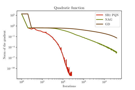
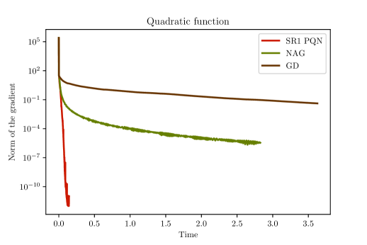
Figure 1: SR1 method significantly outperforms first-order methods in number of iterations and in terms of time.

6.1.1 Logistic regression with a convex regularization

The second experiment is a logistic regression problem with regularization on the benchmark dataset “mushroom” from UCI Machine Learning Repository [49]:

$$\min_{x\in\mathbb{R}^{n}}f(x)\,,\quad\text{with}\ f(x)\coloneqq\frac{1}{m}\sum_{i=1}^{m}\log(1+\exp(-b_{i}a_{i}^{\top}x))+\mu\sqrt{\|x\|^{2}+\epsilon}\,,$$ (179)

where $a_{i}\in\mathbb{R}^{n}$, $b_{i}\in\mathbb{R}$ for $i=1,2,\cdots,m$ denote the given data from the “mushrooms” dataset. We set $\epsilon=1$. The Lipschitz constants are $L=2\sum_{i=1}^{m}\|a_{i}\|^{2}+{\color[rgb]{0,0,0}2\mu}$ and $L_{H}={\color[rgb]{0,0,0}4}$. Here, $m=8124$ and $n=117$. We set $\bar{\kappa}=2L$ for Cubic- and Grad SR1 PQN. The number of restarting steps for Grad SR1 PQN is 1 and the number for Cubic SR1 PQN is 14. We set the stepsize as $1/L$ for NAG and GD. Note that $f$ is coercive and strongly convex on any compact sublevel set. Thus, KŁ inequality holds with respect to $\varphi(t)=ct^{1/2}$ for some $c>0$ and for any $x\in\{x|f(x)\leq f(x_{0})\}$.

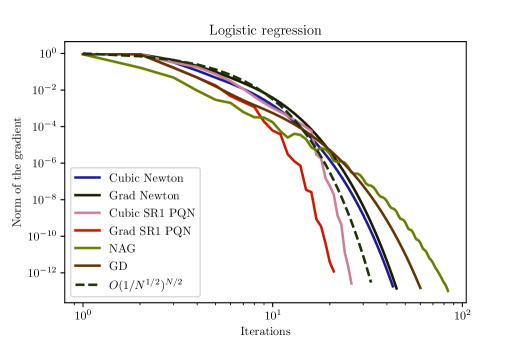
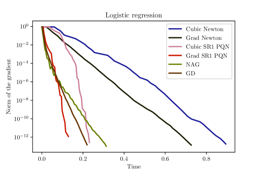
Figure 2: Cubic- and Grad SR1 PQN significantly outperform first-order methods in number of iterations, exhibiting super-linear convergence. In terms of time, Grad SR1 PQN remains one of the fastest methods due to the SR1 metric and the cheap computation of both the correction step and the restarting step.

As depicted in Figure 2, our two regularized quasi Newton methods achieve a super-linear rate of convergence. However, due to the cubic term, neither Cubic Newton nor Cubic quasi-Newton is competitive when it comes to measuring the actual computation time. Gradient regularized SR1 quasi-Newton method outperforms all other first order methods significantly in number of iterations and is among the fastest in terms of time.

6.1.2 Image deblurring problem with a non-convex regularization

The third experiment focuses on an image deblurring problem with a non-convex regularization. Let $b\in\mathbb{R}^{MN}$ represent a blurry and noisy image, where each element $b_{i}$ falls within the range $[0,1]$ for any $i\in\{1\ldots MN\}$. Here, $b$ is constructed by stacking the M columns of length N. To reccover a clean image $x\in\mathbb{R}^{MN}$, we solve the following optimization problem:

$$\min_{x\in\mathbb{R}^{n}}f(x)\,,\quad\text{with}\ f(x)\coloneqq\frac{1}{2}\|Ax-b\|^{2}+\frac{\mu}{2}\log(\rho+\|Kx\|^{2})\,,$$ (180)

where the blurring operator $A\in\mathbb{R}^{MN\times MN}$ is a linear mapping and $Kx$ computes the forward differences in horizontal and vertical direction with $\|K\|\leq 2\sqrt{2}$. We set $\mu=0.001$ and $\rho=0.1$. The Lipschitz constants are estimated from above as $L=\|A\|+5$ and $L_{H}=10$. For this experiment, we take $M=N=64$. Additionally, we set $\bar{\kappa}=2L$ for both Cubic- and Grad SR1 PQN. We set the quasi Newton metric as $\nabla^{2}f(x_{k})$ instead of $LI$ for both the initialization and the restarting steps. In this case, our convergence analysis remains valid. The number of restarting steps for Cubic SR1 PQN is $13$. For nonconvex optimization, we employ a line search with a backtracking strategy for both the gradient descent method (GD_BT) and the Heavy ball method (HB_BT), the latter being a special case of the iPiano algorithm from [41]). Figure 3 exhibits the comparison between our cubic SR1 method and GD_BT and HB_BT .

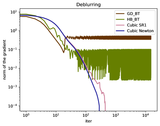
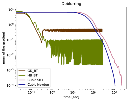
Figure 3: In the number of iterations and the norm of the gradients, Cubic Newton and Cubic SR1 attain higher accuracy eventually. Moreover, both cubic Newton and Cubic SR1 show more stable convergence, compared to first order methods that utilize line search.

As illustrated in Figure 3, our Cubic SR1 maintains superlinear convergence, despite slightly slower than the cubic Newton method. In the case when only the first order information is accessible, Cubic SR1 offers a more practical alternative. Both regularized second order methods are more stable than first order method with Armijo line search when applied on this nonconvex problem. The oscillation in the latter methods may be attributed to the allowance of a large step size and a sharp local minimum of the nonconvex function.

7 Conclusion

In this paper, we study two regularized proximal quasi-Newton SR1 methods which converge with explicit (non-asymptotic) super-linear rates even for some classes of non-convex optimization problems. The key is the adaptation of convergence analysis from the work [51] on strongly convex problems to non-convex problems, illustrating the power of the trace potential function $V(G)=\mathrm{tr}\,G$. Moreover, our algorithm and analysis is directly developed for non-smooth additive composite problems. The analysis of convergence used in this paper, for the first time, reveals the possibility to study non-asymptotic super-linear convergence rates of classical quasi Newton schemes without assuming strong convexity. This work shows that KŁ property, which can be observed in many non-convex problems, is an important generalization of the strong convexity to study quasi Newton methods and we can expect more results similar as in strongly convex cases.

Appendix A Convergence of cubic quasi Newton SR1 method with Łojasiewicz inequality

Assumption 3.

$f$ satisfies $1/2$-Łojasiewicz inequality with constant $\mu$, i.e., there exists a constant $\mu$ such that for any $x\in\mathbb{R}^{n}$, we have

$$f(x)-\inf f\leq\frac{1}{2\mu}\|\nabla f(x)\|^{2}\,.$$ (181)

Remark A.1.

This assumption is equivalent to assume $f$ has the quadratic growth rate, i.e., $f(x)-\min f\geq c(\mathrm{dist}(x,\operatorname*{argmin}f))^{2}$ for some constant $c>0$. For non-smooth case, it corresponds to assuming that the objective function has KL exponent $1/2$.

In order to solve the problem in (4) with $g=0$ and f satisfying Łojasiewicz inequality, we employ the same cubic regularized SR1 quasi-Newton method (Algorithm 3). Algorithm 3 (Cubic SR1) is the same with the first algorithm proposed in previous section where $g=0$.

Algorithm 3 Cubic SR1 QN

$x_{0}$, $G_{0}=LI$, $r_{-1}=0$.

Update for $k=0,\cdots,N$:

1. Update

   $$\begin{split}x_{k+1}&=\operatorname*{argmin}_{x\in\mathbb{R}^{n}}\;\{\left\langle\nabla f(x_{k}),x-x_{k}\right\rangle+\frac{1}{2}\|x-x_{k}\|_{(G_{k}+L_{H}r_{k-1}I)}^{2}+{\frac{L_{H}}{3}\|x-x_{k}\|^{3}}\}.\\ \end{split}$$

2. Set $u_{k}=x_{k+1}-x_{k}$, $r_{k}=\|u_{k}\|$, $\lambda_{k}=L_{H}r_{k-1}+L_{H}r_{k}$.

3. Compute $\tilde{G}_{k+1}=G_{k}+\lambda_{k}I$ and

   $$F^{\prime}(x_{k+1})=\nabla f(x_{k+1})-\nabla f(x_{k})-\tilde{G}_{k+1}u_{k}\,.$$

4. Compute $G_{k+1}=\text{SR1}(J_{k},\tilde{G}_{k+1},u_{k})$ ($J_{k}\coloneqq\int_{0}^{1}\nabla^{2}f(x_{k}+tu_{k})dt$).

5. If $\|F^{\prime}(x_{k+1})\|=0$: Terminate.

End

Theorem A.2.

Let Assumption 3 hold and $g=0$. For any initialization $x_{0}\in\mathbb{R}^{n}$ and any $N\in\mathbb{N}$, Cubic SR1 QN has a global convergence with the rate:

$$\|\nabla f(x_{N})\|\leq\frac{6}{\mu}\left(\frac{C}{N^{1/3}}\right)^{N/2}\|\nabla f(x_{0})\|\,,$$

where $C=\left(2nL+nd+2nL_{H}\left(\frac{6}{L_{H}}\left(f(x_{0})-\inf f\right)\right)^{1/3}\right)$ and $d$ is the diameter of the sub-level set $\{x|f(x)\leq f(x_{0})\}$.

A.1 Convergence analysis of Algorithm 3

The optimality condition of the update step in (1) is

$$\nabla f(x_{k})+(G_{k}+L_{H}r_{k-1})(x_{k+1}-x_{k})+L_{H}\|x_{k+1}-x_{k}\|(x_{k+1}-x_{k})\ni 0\,,$$ (182)

which, using our notations, simplifies to

$$\nabla f(x_{k})+\underbrace{(G_{k}+\lambda_{k})}_{\tilde{G}_{k+1}}(x_{k+1}-x_{k})\ni 0\,.$$ (183)

Surprisingly, using our notations, $\tilde{G}_{k+1}=(G_{k}+\lambda_{k})$.

Lemma A.3.

For any $k\in\mathbb{N}$, we have

$${\tilde{G}_{k+1}}\succeq G_{k+1}\succeq J_{k}$$ (184)

Proof.

We argue by induction. When $k=0$, we have $G_{0}=LI\succeq J_{0}$ and $\tilde{G}_{1}\succeq J_{0}$. Then, $\tilde{G}_{1}\succeq G_{1}\succeq J_{0}$, thanks to Lemma 5.4. We assume the inequality holds for $k$, namely, $\tilde{G}_{k}\succeq G_{k}\succeq J_{k-1}$. Thus, for $k+1$, we deduce that ${\tilde{G}_{k+1}}=G_{k}+L_{H}(r_{k}+r_{k-1})I\succeq J_{k-1}+L_{H}(r_{k}+r_{k-1})\succeq J_{k}$. Thanks to Lemma 5.4, we obtain ${\tilde{G}_{k+1}}\succeq G_{k+1}\succeq J_{k}$. Therefore, $\mathrm{tr}\,\tilde{G}_{k+1}\geq\mathrm{tr}\,G_{k+1}$. ∎

Lemma A.4.

For each $k\in\mathbb{N}$, we have

$$f(x_{k+1})-f(x_{k})\leq-\frac{L_{H}}{6}r_{k}^{3}\,,$$

$$\left\langle({\tilde{G}_{k+1}}-J_{k})u_{k},u_{k}\right\rangle\leq\frac{6}{\mu}\|\nabla f(x_{k})\|^{2}\,.$$

Proof.

We start with showing the first result. The update step 1 implies that

$$f(x_{k})+\left\langle\nabla f(x_{k}),u_{k}\right\rangle+\frac{1}{2}\left\langle(G_{k}+L_{H}r_{k-1})u_{k},u_{k}\right\rangle+\frac{L_{H}}{3}r_{k}^{3}\leq f(x_{k})\,.$$ (185)

Then, thanks to Lemma 5.1, we have

$$f(x_{k+1})-f(x_{k})\leq\left\langle\nabla f(x_{k}),u_{k}\right\rangle+{\frac{1}{2}}\left\langle\nabla^{2}f(x_{k})u_{k},u_{k}\right\rangle+\frac{L_{H}}{6}\|u_{k}\|^{3}\,.$$ (186)

Combining two inequalities above, we can obtain that

$$\begin{split}f(x_{k+1})&\leq f(x_{k})+\frac{1}{2}\left\langle\nabla^{2}f(x_{k})u_{k},u_{k}\right\rangle-\frac{1}{2}\left\langle(G_{k}+L_{H}r_{k-1})u_{k},u_{k}\right\rangle-\frac{L_{H}}{6}\|u_{k}\|^{3}\\ &\leq f(x_{k})-\frac{L_{H}}{6}r_{k}^{3}\,,\\ \end{split}$$ (187)

where the last inequality holds thanks to the fact $G_{k}+L_{H}r_{k-1}I\succeq J_{k-1}+\frac{L_{H}}{2}r_{k-1}I\succeq\nabla^{2}f(x_{k})$ (see Lemma 5.3). For the second result, we need another inequality from Lemma 5.1:

$$f(x_{k+1})-f(x_{k})\leq\left\langle\nabla f(x_{k}),u_{k}\right\rangle+{\frac{1}{2}}\left\langle J_{k}u_{k},u_{k}\right\rangle+\frac{L_{H}}{6}\|u_{k}\|^{3}\,.$$ (188)

Adding (185) to (188), we obtain that

$$\left\langle({\tilde{G}_{k+1}}-J_{k})u_{k},u_{k}\right\rangle\leq 2(f(x_{k})-f(x_{k+1}))+\frac{2L_{H}}{3}r_{k}^{3}\,.$$ (189)

Combining the first result above, we can derive that

$$\begin{split}\left\langle({\tilde{G}_{k+1}}-J_{k})u_{k},u_{k}\right\rangle&\leq 2(f(x_{k})-f(x_{k+1}))+\frac{2L_{H}}{3}r_{k}^{3}\\ &\leq 6(f(x_{k})-f(x_{k+1}))\leq{6(f(x_{k})-\inf f)}\\ &\leq\frac{6}{\mu}\|\nabla f(x_{k})\|^{2}\,,\\ \end{split}$$ (190)

where the last inequality utilizes Łojasiewicz ineqality. ∎

Lemma A.5.

Given a number of iterations $N\in\mathbb{N}$, we have:

$$\sum_{k=0}^{N}r_{k}^{3}\leq\frac{6(F(x_{0})-\inf F)}{L_{H}}<+\infty\,,$$ (191)

$$\sum_{k=0}^{N-1}r_{k}\leq C_{0}N^{\frac{2}{3}}\,,$$ (192)

$$\sum_{k=1}^{N}r_{k}\leq C_{0}N^{\frac{2}{3}}\,,$$ (193)

where $C_{0}\coloneqq(\frac{6(F(x_{0})-\inf F)}{L_{H}})^{1/3}$.

Proof.

The first inequality is derived from Lemma A.4. Then, we apply the Cauchy–Schwarz inequality and obtain

$$\sum_{i=0}^{N-1}r_{k}\leq\left(\sum_{k=0}^{N-1}r_{k}^{3}\right)^{1/3}\left(\sum_{i=0}^{N-1}1^{\frac{3}{2}}\right)^{2/3}\leq\left(\sum_{k=0}^{\infty}r_{k}^{3}\right)^{1/3}N^{2/3}\leq C_{0}N^{2/3}\,.$$ (194)

Similarly, we have

$$\sum_{i=1}^{N}r_{k}\leq\left(\sum_{k=1}^{N}r_{k}^{3}\right)^{1/3}\left(\sum_{i=1}^{N}1^{\frac{3}{2}}\right)^{2/3}\leq\left(\sum_{k=0}^{\infty}r_{k}^{3}\right)^{1/3}N^{2/3}\leq C_{0}N^{2/3}\,.$$ (195)

∎

Lemma A.6.

$$V(\tilde{G}_{k+1})-V(\tilde{G}_{k+2})\geq\frac{\mu g^{2}_{k+1}}{6g_{k}^{2}}-n\lambda_{k+1}\,,$$ (196)

where $g_{k}\coloneqq\|\nabla f(x_{k})\|$.

Proof.

Wlog, we assume $(\tilde{G}_{k+1}-J_{k})u\neq 0$.

$$V(\tilde{G}_{k+1})-V(G_{k+1})=\nu(J_{k},\tilde{G}_{k+1},u_{k})=\frac{u_{k}^{\top}(\tilde{G}_{k+1}-J_{k})(\tilde{G}_{k+1}-J_{k})u_{k}}{u_{k}^{\top}(\tilde{G}_{k+1}-J_{k})u_{k}}\,,$$

Using the definition of $\tilde{G}_{k+1}$, we have $(\tilde{G}_{k+1}-J_{k})u_{k}=\nabla f(x_{k})-\nabla f(x_{k+1})-\nabla f(x_{k})=-\nabla f(x_{k+1})$. Thanks to the second inequality from Lemma A.4, we obtain

$$\nu(J_{k},\tilde{G}_{k+1},u_{k})\geq\frac{\mu\|\nabla f(x_{k+1})\|^{2}}{6\|\nabla f(x_{k})\|^{2}}\,.$$

On the other hand,

$$V(G_{k+1})-V(\tilde{G}_{k+2})=-n\lambda_{k+1}\,.$$

∎

Theorem A.7.

For any initialization $x_{0}\in\mathbb{R}^{n}$ and any $N\in\mathbb{N}$, Cubic SR1 QN has a global convergence with the rate:

$$\|\nabla f(x_{N})\|\leq\frac{6}{\mu}\left(\frac{C}{N^{1/3}}\right)^{N/2}\|\nabla f(x_{0})\|\,,$$

where $C=\left(2nL+2nL_{H}d+2nL_{H}\left(\frac{6}{L_{H}}\left(f(x_{0})-\inf f\right)\right)^{1/3}\right)$. Here, $d$ is the diameter of the sub-level set $\{x|f(x)\leq f(x_{0})\}$.

Proof of Theorem A.2.

Summing up the following inequalities from $k=0$ to $k=N-1$

$$V(\tilde{G}_{k+1})-V(\tilde{G}_{k+2})\geq\frac{\mu g^{2}_{k+1}}{6g_{k}^{2}}-n\lambda_{k+1}\,,$$

we have

$$V(\tilde{G}_{1})-V(\tilde{G}_{N})+n\sum_{k=0}^{N-1}\lambda_{k}\geq\sum_{k=0}^{N-1}\frac{\mu g^{2}_{k+1}}{6g_{k}^{2}}\,.$$

Thanks to Lemma A.3, $V(\tilde{G}_{N})\geq V(J_{N-1})\geq-nL$, $V(\tilde{G}_{1})\leq nL+2nL_{H}d$. According to Lemma A.5, $\sum_{k=1}^{N}\lambda_{k}\leq 2L_{H}C_{0}(N^{2/3})$. Here, $d$ is the diameter of the sub-level set $\{x|f(x)\leq f(x_{0})\}$. Dividing both sides by $N$ and using the concavity of $\log$, we have

$$\begin{split}\log\left(\frac{1}{N}\left(2nL+2nL_{H}d+2L_{H}C_{0}(N^{2/3})\right)\right)\geq\log\left(\frac{1}{N}\left(\sum_{k=0}^{N}\frac{\mu g^{2}_{k+1}}{6g_{k}^{2}}\right)\right)&\geq\left(\frac{1}{N}\sum_{k=0}^{N}\log\left(\frac{\mu g^{2}_{k+1}}{6g_{k}^{2}}\right)\right)\\ &\geq\log\left(\frac{\mu}{6}\left(\frac{g_{N}}{g_{0}}\right)^{2/N}\right)\,.\\ \end{split}$$ (197)

∎

REFERENCES

• [1] H. Attouch, J. Bolte, P. Redont, and A. Soubeyran, Proximal alternating minimization and projection methods for nonconvex problems: An approach based on the kurdyka-Lojasiewicz inequality, Mathematics of operations research, 35 (2010), pp. 438–457.
• [2] S. Becker and J. Fadili, A quasi-Newton proximal splitting method, Advances in neural information processing systems, 25 (2012).
• [3] S. Becker, J. Fadili, and P. Ochs, On quasi-Newton forward-backward splitting: proximal calculus and convergence, SIAM Journal on Optimization, 29 (2019), pp. 2445–2481.
• [4] H. Y. Benson and D. F. Shanno, Cubic regularization in symmetric rank-1 quasi-Newton methods, Mathematical Programming Computation, 10 (2018), pp. 457–486.
• [5] T. Bianconcini, G. Liuzzi, B. Morini, and M. Sciandrone, On the use of iterative methods in cubic regularization for unconstrained optimization, Computational Optimization and Applications, 60 (2015), pp. 35–57.
• [6] J. Bolte, A. Daniilidis, and A. Lewis, The Lojasiewicz inequality for nonsmooth subanalytic functions with applications to subgradient dynamical systems, SIAM Journal on Optimization, 17 (2007), pp. 1205–1223.
• [7] J. Bolte, A. Daniilidis, A. Lewis, and M. Shiota, Clarke subgradients of stratifiable functions, SIAM Journal on Optimization, 18 (2007), pp. 556–572.
• [8] J. Bolte, A. Daniilidis, O. Ley, and L. Mazet, Characterizations of Lojasiewicz inequalities and applications, arXiv preprint arXiv:0802.0826, (2008).
• [9] J. Bolte, S. Sabach, and M. Teboulle, Proximal alternating linearized minimization for nonconvex and nonsmooth problems, Mathematical Programming, 146 (2014), pp. 459–494.
• [10] C. G. Broyden, Quasi-Newton methods and their application to function minimisation, Mathematics of Computation, 21 (1967), pp. 368–381.
• [11] C. G. Broyden, The convergence of a class of double-rank minimization algorithms 1. general considerations, IMA Journal of Applied Mathematics, 6 (1970), pp. 76–90.
• [12] C. G. Broyden, J. E. Dennis Jr, and J. J. Moré, On the local and superlinear convergence of quasi-Newton methods, IMA Journal of Applied Mathematics, 12 (1973), pp. 223–245.
• [13] C. Cartis, N. I. Gould, and P. L. Toint, Adaptive cubic regularisation methods for unconstrained optimization. part i: motivation, convergence and numerical results, Mathematical Programming, 127 (2011), pp. 245–295.
• [14] H. Chen, W.-H. Lam, and S.-C. Chan, On the convergence analysis of cubic regularized symmetric rank-1 quasi-Newton method and the incremental version in the application of large-scale problems, IEEE Access, 7 (2019), pp. 114042–114059.
• [15] X. Chen and M. Fukushima, Proximal quasi-Newton methods for nondifferentiable convex optimization, Mathematical Programming, 85 (1999), pp. 313–334.
• [16] W. C. Davidon, Variable metric method for minimization, SIAM Journal on optimization, 1 (1991), pp. 1–17.
• [17] J. E. Dennis and R. B. Schnabel, Numerical Methods for Unconstrained Optimization and Nonlinear Equations, Society for Industrial and Applied Mathematics, 1996.
• [18] J. E. Dennis, Jr and J. J. Moré, Quasi-Newton methods, motivation and theory, SIAM review, 19 (1977), pp. 46–89.
• [19] L. Dixon, Quasi Newton techniques generate identical points ii: the proofs of four new theorems, Mathematical Programming, 3 (1972), pp. 345–358.
• [20] N. Doikov and Y. Nesterov, Gradient regularization of Newton method with Bregman distances, Mathematical programming, 204 (2024), pp. 1–25.
• [21] R. Fletcher, A new approach to variable metric algorithms, The computer journal, 13 (1970), pp. 317–322.
• [22] R. Fletcher and M. J. Powell, A rapidly convergent descent method for minimization, The computer journal, 6 (1963), pp. 163–168.
• [23] P. Frankel, G. Garrigos, and J. Peypouquet, Splitting methods with variable metric for kurdyka–Lojasiewicz functions and general convergence rates, Journal of Optimization Theory and Applications, 165 (2015), pp. 874–900.
• [24] D. Goldfarb, A family of variable-metric methods derived by variational means, Mathematics of computation, 24 (1970), pp. 23–26.
• [25] N. I. Gould, M. Porcelli, and P. L. Toint, Updating the regularization parameter in the adaptive cubic regularization algorithm, Computational optimization and applications, 53 (2012), pp. 1–22.
• [26] G. N. Grapiglia, M. L. Gonçalves, and G. Silva, A cubic regularization of Newton’s method with finite difference hessian approximations, Numerical Algorithms, (2022), pp. 1–24.
• [27] Q. Jin, R. Jiang, and A. Mokhtari, Non-asymptotic global convergence analysis of BFGS with the Armijo-Wolfe line search, arXiv preprint arXiv:2404.16731, (2024).
• [28] Q. Jin and A. Mokhtari, Non-asymptotic superlinear convergence of standard quasi-Newton methods, Mathematical Programming, 200 (2023), pp. 425–473.
• [29] D. Kamzolov, K. Ziu, A. Agafonov, and M. Takác, Cubic regularized quasi-newton methods, arXiv preprint arXiv:2302.04987, (2023).
• [30] C. Kanzow and T. Lechner, Efficient regularized proximal quasi-Newton methods for large-scale nonconvex composite optimization problems, arXiv preprint arXiv:2210.07644, (2022).
• [31] H. Karimi, J. Nutini, and M. Schmidt, Linear convergence of gradient and proximal-gradient methods under the Polyak-Lojasiewicz condition, in Machine Learning and Knowledge Discovery in Databases: European Conference, ECML PKDD 2016, Riva del Garda, Italy, September 19-23, 2016, Proceedings, Part I 16, Springer, 2016, pp. 795–811.
• [32] S. Karimi and S. Vavasis, IMRO: A proximal quasi-Newton method for solving $\ell_{1}$-regularized least squares problems, SIAM Journal on Optimization, 27 (2017), pp. 583–615.
• [33] J. D. Lee, Y. Sun, and M. Saunders, Proximal Newton-type methods for convex optimization, Advances in Neural Information Processing Systems, 25 (2012).
• [34] K. LEVENBERG, A method for the solution of certain non-linear problems in least squares, Quarterly of Applied Mathematics, 2 (1944), pp. 164–168.
• [35] G. Li and T. K. Pong, Calculus of the exponent of kurdyka–Lojasiewicz inequality and its applications to linear convergence of first-order methods, Foundations of computational mathematics, 18 (2018), pp. 1199–1232.
• [36] S. Lu, Z. Wei, and L. Li, A trust region algorithm with adaptive cubic regularization methods for nonsmooth convex minimization, Computational Optimization and Applications, 51 (2012), pp. 551–573.
• [37] D. W. Marquardt, An algorithm for least-squares estimation of nonlinear parameters, Journal of the society for Industrial and Applied Mathematics, 11 (1963), pp. 431–441.
• [38] K. Mishchenko, Regularized Newton method with global convergence, SIAM Journal on Optimization, 33 (2023), pp. 1440–1462.
• [39] Y. Nesterov and B. T. Polyak, Cubic regularization of Newton method and its global performance, Mathematical programming, 108 (2006), pp. 177–205.
• [40] J. Nocedal and S. J. Wright, Numerical Optimization, Springer, New York, NY, USA, 2e ed., 2006.
• [41] P. Ochs, Y. Chen, T. Brox, and T. Pock, ipiano: Inertial proximal algorithm for nonconvex optimization, SIAM Journal on Imaging Sciences, 7 (2014), pp. 1388–1419.
• [42] Y. Qian and S. Pan, A superlinear convergence framework for Kurdyka-Lojasiewicz optimization, arXiv e-prints, (2022), pp. arXiv–2210.
• [43] R. T. Rockafellar and R. J.-B. Wets, Variational analysis, vol. 317, Springer Science & Business Media, 2009.
• [44] A. Rodomanov, Global complexity analysis of BFGS, arXiv preprint arXiv:2404.15051, (2024).
• [45] A. Rodomanov and Y. Nesterov, Greedy quasi-Newton methods with explicit superlinear convergence, SIAM Journal on Optimization, 31 (2021), pp. 785–811.
• [46]  , Rates of superlinear convergence for classical quasi-Newton methods, Mathematical Programming, (2022), pp. 1–32.
• [47] K. Scheinberg and X. Tang, Practical inexact proximal quasi-Newton method with global complexity analysis, Mathematical Programming, 160 (2016), pp. 495–529.
• [48] L. Stella, A. Themelis, and P. Patrinos, Forward–backward quasi-newton methods for nonsmooth optimization problems, Computational Optimization and Applications, 67 (2017), pp. 443–487.
• [49] Mushroom. UCI Machine Learning Repository, 1981. DOI: https://doi.org/10.24432/C5959T.
• [50] S. Wang, J. Fadili, and P. Ochs, Inertial quasi-Newton methods for monotone inclusion: efficient resolvent calculus and primal-dual methods, arXiv preprint arXiv:2209.14019, (2022).
• [51]  , Global non-asymptotic super-linear convergence rates of regularized proximal quasi-newton methods on non-smooth composite problems, arXiv preprint arXiv:2410.11676, (2024).
• [52] H. Ye, D. Lin, X. Chang, and Z. Zhang, Towards explicit superlinear convergence rate for SR1, Mathematical Programming, 199 (2023), pp. 1273–1303.
• [53] H. Zhang, New analysis of linear convergence of gradient-type methods via unifying error bound conditions, Mathematical Programming, 180 (2020), pp. 371–416.