Symbolic Higher-Order Analysis of Multivariate Time Series

Abstract

Identifying patterns of relations among the units of a complex system from measurements of their activities in time is a fundamental problem with many practical applications. Here, we introduce a method that detects dependencies of any order in multivariate time series data. The method first transforms a multivariate time series into a symbolic sequence, and then extract statistically significant strings of symbols through a Bayesian approach. Such motifs are finally modelled as the hyperedges of a hypergraph, allowing us to use network theory to study higher-order interactions in the original data. When applied to neural and social systems, our method reveals meaningful higher-order dependencies, highlighting their importance in both brain function and social behaviour.

Introduction.

Complex systems exhibit collective behaviours of extraordinary richness. Notable examples include the emergence of cooperation [1, 2] and epidemics in social groups [3], as well as synchronization in biological systems [4] and in human cognition [5]. Such behaviors directly stem from the interactions between the many fundamental units of such systems, e.g. individuals in a society or neurons within the brain [6, 7, 8, 9]. The most intuitive way to represent interactions in a complex system is through a network whose nodes correspond to the fundamental units of the complex systems and the edges describe direct or indirect couplings, or other dependencies or correlations between two units [10, 11, 12]. However, networks often provide an oversimplified description of a complex system in terms of pairwise relations. In many cases, units interact in groups, and these group interactions cannot be reduced to pairwise relationships among group members [13]. Higher-order (HO) representations of the interaction structure, such as simplicial complexes and hypergraphs, recently have been extensively and successfully applied to the study of complex systems [14, 15, 16, 17, 18, 19, 20, 21, 22, 23, 24]. In many cases, the interactions within a complex system must be inferred directly from the observation of the system dynamics, specifically from multivariate time series obtained by measuring the activity of each of the units of the system. Given the importance of the problem, numerous methods have been developed over the years to reconstruct pairwise networks from such empirical time-series data [25, 26, 27, 28, 29]. In contrast, efforts to reconstruct or filter higher-order interactions have only emerged more recently [30, 31, 32, 33, 34, 35, 36, 37, 38, 39]. Existing approaches typically rely on one of the following: the assumption of continuous, differentiable time series [33, 34]; discretized versions of continuous time series with specific statistical properties (e.g., normally distributed values) [35, 37, 38], or prior knowledge of the system’s underlying dynamical process and its functional form [33, 39]. These assumptions are often too restrictive in real-world scenarios, where the exact dynamical rules generating the time series are unknown [34], and the distribution of values across real-world datasets can be highly heterogeneous [40]. Additionally, the activity of individual units is frequently neither continuous nor differentiable; instead, it tends to occur at discrete moments in time, with events that are effectively instantaneous relative to the typical timescale of observation. Relevant examples are the spiking activity of neurons, seismic events, user activity on social platforms and sell-buy orders in stock markets. In all such cases, the dynamics is better described by a set of binary time series data of $0$ and $1$, where the $1$ states represent the given points in time at which the highly localized events occur.

In this Letter, we introduce a general and scalable method to identify higher-order relations in multivariate discrete time series. The method does not require any assumption on the underlying dynamics and is specifically designed for, and naturally applies to, all the systems described above. The method works in the following way: first, the original discrete multivariate time series is mapped into a sequence of symbols; then, Bayesian statistics is used to infer the significant patterns of symbols and their higher-order organization. In this way, the approach combines the descriptive power of symbolic dynamics [41, 42] with the flexibility of Bayesian methods and with the high capability of hypergraphs in modelling complex interactions. While the framework is here presented for binary time series, it readily extends to any discrete-valued time series, as any time series with discrete states can be trivially decomposed into a larger collection of binary time series. Moreover, although the method is naturally suited to time series with a finite number of states, it can also be applied to continuous signals through appropriate thresholding.

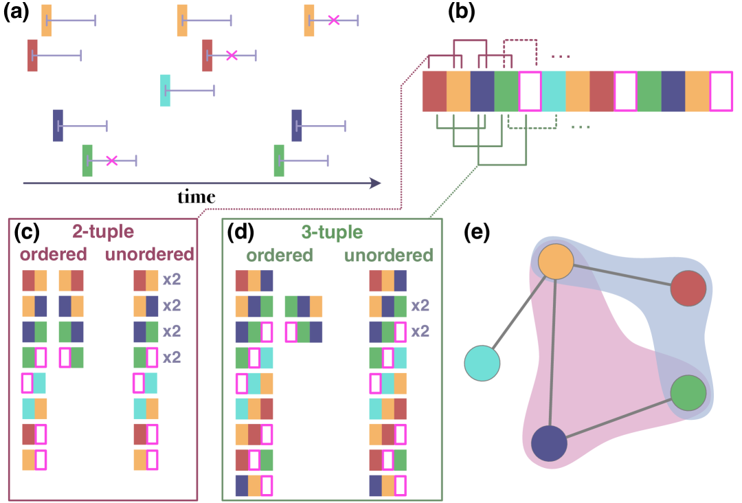
Figure 1: (a)  Each time series $x_{i}(t)$, with $i=1,\ldots N$, is associated to one of $N$ different symbols/colours. (b) Then the set of time series is converted into a symbolic sequence: if an event $x_{i}(t)=1$ is followed by $x_{j}(t)=1$ within a time interval $\Delta t$ (grey bar in (a)), their corresponding symbols are placed adjacently in the symbolic sequence. Otherwise (pink cross) a “space” symbol is inserted in the sequence. (c-d) Lists of ordered and unordered $2$-tuples and $3$-tuples found in the sequence. (e) Statistically significant tuples (motifs) are finally the hyperedges of an hypergraph.

Method.

Let us consider a multivariate time series of $N$ binary signals $x_{i}(t)\in\{0,1\},\forall i=1,...,N$, with $t\in[0,T]$, where $x_{i}(t)=1$ represents the occurrence of event of type $i$ at time $t$, and $T$ is the observation time. We want to construct a hypergraph whose $N$ nodes are associated with the different types of events, and the hyperedges represent groups of correlated events. In order to do this, we first convert the multivariate time series into a symbolic sequence, Fig. 1(a,b). We consider an alphabet $\cal A$ of $N+1$ symbols, the first $N$ symbols (colours in Figure) respectively associated to each one of the $N$ time series, plus a special “space” (or empty) symbol. We then construct an ordered sequence $\cal S$ of such symbols from the original set of $N$ time series in the following way. When the event $x_{i}(t)=1$ is followed by the event $x_{j}(t^{\prime})=1$ within a given time interval $\Delta t$ (i.e., when $t^{\prime}-t<\Delta t$), the symbols corresponding to $i$ and $j$ are placed in adjacent positions in the symbolic sequence $\cal S$. If instead no activity occurs within $\Delta t$, the space symbol is inserted in the sequence after $i$. Finally, from the symbolic sequence $\cal{S}$, we extract the multiset (i.e., with repetitions of elements) $\mathcal{D}^{l}$ of all overlapping $l$-tuples, with cardinality $|\mathcal{D}^{l}|=M^{l}$, and the set $\mathcal{T}^{l}$ of the unique $l$-tuples (without repetition), with cardinality $|\mathcal{T}^{l}|=N^{l}$, see Fig. 1(c,d). A $l$-tuple $\bm{s}=(s_{1},s_{2},\dots,s_{l})\in\mathcal{T}^{l}$ is an ordered (or unordered) sequence of $l$ symbols $s_{i}\in\mathcal{A}~\forall i=1,2,\ldots l$. In this way, from a sequence $\mathcal{S}$ of length $S$, we get $M^{l}=S-l+1$ tuples of length $l$.

This approach allows to build a hypergraph $\mathcal{H}(\mathcal{N},\mathcal{E})$ of higher-order correlations in the original multivariate time-series. The $N$ nodes of the hypergraph correspond to the $N$ units (time series), i.e. the different types of possible events. The hyperedges of different sizes $l$, with $l\geq 2$, representing groups of $l$ units whose dynamics are correlated, are defined by the $l$-motifs in $\cal S$, i.e. by the statistically significant $l$-tuples of symbols. This is shown in Fig. 1(e) for the case of $l=2$ and $3$. In order to assess the significance of a $l$-tuple $\bm{s}$, we evaluate the expected probability $p_{\text{exp}}(\bm{s})$ from the observed occurrences of tuples of shorter length:

$$p_{\text{exp}}(\bm{s}=s_{1},s_{2}) =p_{\text{obs}}(s_{1})p_{\text{obs}}(s_{2})$$ (1)

and:

$$p_{\text{exp}}(\bm{s}=s_{1},\dots,s_{l}) =\frac{p_{\text{obs}}(s_{1},\dots,s_{l-1})p_{\text{obs}}(s_{2},\dots,s_{l})}{p_{\text{obs}}(s_{2},\dots,s_{l-1})}$$ (2)

for $l>2$. The observed probability of $\bm{s}$ in the equations above is computed as:

$$p_{\text{obs}}(\bm{s})=\frac{n_{\text{obs}}(\bm{s})}{\sum_{s\in\mathcal{T}^{l}}n_{\text{obs}}(\bm{s})}=\frac{n_{\text{obs}}(\bm{s})}{S-l+1}$$ (3)

where $n_{\text{obs}}(\bm{s})$ counts the number of occurrences of $\bm{s}$ in $\mathcal{D}^{l}$ and therefore satisfies $\sum_{s\in\mathcal{T}^{l}}n_{\text{obs}}(\bm{s})=S-l+1$. In this way, when evaluating $p_{\text{exp}}(\bm{s})$, we take into account the effect of lower-order correlations coming from tuples of length smaller than $l$ [43]. If we are interested in the case of unordered tuples, we can simply sum over $S_{p}(\bm{s})$, the set of unique permutations $\bm{\sigma}$ of the ordered tuple $\bm{s}=s_{1},\dots,s_{l}$, obtaining: $p_{\text{exp}}^{\text{und}}(\bm{s})=\sum_{\bm{\sigma}\in S_{p}(\bm{s})}p_{\text{exp}}(\bm{\sigma})$ and $n_{\text{obs}}^{\text{und}}(\bm{s})=\sum_{\bm{\sigma}\in S_{p}(\bm{s})}n_{\text{obs}}(\bm{\sigma})$, where $p_{\text{exp}}(\bm{\sigma})$ and $n_{\text{obs}}(\bm{\sigma})$ are respectively the expected probability and the observed occurrences of the permutation $\bm{\sigma}$ for the ordered case.

We then use a Bayesian approach to reject or accept the null hypothesis that each $l$-tuple $\bm{s}_{i}\in\mathcal{T}^{l}$ where $i\in 1,\dots,N^{l}$ appears with probability $p_{\text{exp}}(\bm{s}_{i})$. Let us define the vector of the observed count of $l$-tuples in $\mathcal{S}$: $\mathbf{n}^{l}_{\text{obs}}=\left[n_{\text{obs}}(\bm{s}_{1}),\dots,n_{\text{obs}}(\bm{s}_{N^{l}})\right]$, where $n_{\text{obs}}(\bm{s}_{i})$ is the number of times each unique tuple $\bm{s}_{i}\in\mathcal{T}^{l}$ is repeated in $\mathcal{D}^{l}$. We assume that each $l$-tuple represents the outcome of a random experiment over $S-l+1$ independent trials. That is, the outcome of each trial can be tuple $\bm{s}_{i}\in\mathcal{T}^{l}$ with probability $p(\bm{s}_{i})$, such that $\sum_{i}p(\bm{s}_{i})=1$. Under this assumption, the likelihood of $\mathbf{n}^{l}_{\text{obs}}=\left[n_{\text{obs}}(\bm{s}_{1}),...,n_{\text{obs}}(\bm{s}_{N^{l}})\right]$ is a multinomial distribution:

$$\mathcal{L}(\mathbf{n}_{\text{obs}}^{l}\mid\mathbf{p}^{l})=\frac{(S-l+1)!}{\prod_{i=1}^{N^{l}}n_{\text{obs}}(\bm{s}_{i})!}\prod_{i=1}^{N^{l}}p(\bm{s}_{i})^{n_{\text{obs}}(\bm{s}_{i})}$$ (4)

where $\mathbf{p}^{l}=\left[p(\bm{s}_{1}),\dots,p(\bm{s}_{N^{l}})\right]$ is the vector of the occurrence probability of each tuple. For the prior $\Pi(\mathbf{p}^{l})$, as commonly done, we take the conjugate distribution of the multinomial distribution, that is the Dirichlet distribution:

$$\Pi(\mathbf{p}^{l})= \text{Dirichlet}(\alpha_{1}^{l},\alpha_{2}^{l},\dots,\alpha_{N^{l}}^{l})$$

$$= \frac{\Gamma\left(\sum_{i=1}^{N^{l}}\alpha_{i}^{l}\right)}{\prod_{i=1}^{N^{l}}\Gamma(\alpha_{i}^{l})}\prod_{i=1}^{N^{l}}p(\alpha_{i}^{l})^{\alpha_{i}^{l}-1}$$ (5)

where $\alpha_{i}^{l}$ is the concentration parameter of the tuple $\bm{s}_{i}$, which can be interpreted as prior counts or pseudo-counts, and $\Gamma(\cdot)$ is the Gamma function. We adopt an empirical Bayes approach, where part of the information of the data is used to compute the prior. Namely, to compute the concentration parameter of an $l$-tuple, we use the expected probability in Eqs. (1),(2), functions of the observed probability of $l-1$ and $l-2$-tuples: $\alpha_{i}^{l}=n_{\text{exp}}(\bm{s}_{i})+\epsilon$. Here, $n_{\text{exp}}(\bm{s}_{i})=p_{\text{exp}}(\bm{s}_{i})(S-l+1)$ is the expected number of occurrences of the $l$-tuple $\bm{s}_{i}$ in the sequence, and $\epsilon\geq 0$ is a regularization parameter (a minimum number of pseudo-counts) that ensures that the prior is not too confident, in particular for very small $n_{\text{exp}}(\bm{s}_{i})$, and allows for Bayesian updating. For our results we choose $\epsilon=1$. We then use the likelihood to update the prior obtaining the posterior $P(p\mid\text{Data})$ which, given that the multinomial and the Dirichlet distributions are conjugate, is also a Dirichlet distribution:

$$P(\mathbf{p}\mid\text{Data})=\text{Dirichlet}( \alpha_{1}^{l}+n_{\text{obs}}(\bm{s}_{1}),\alpha_{2}^{l}+n_{\text{obs}}(\bm{s}_{2}),$$

$$\dots,\alpha_{N^{l}}^{l}+n_{\text{obs}}(\bm{s}_{N^{l}}))$$ (6)

To assess the significance of the $l$-tuple $\bm{s}_{i}$, we compute the Jensen-Shannon distance $d_{\text{JS}}(\bm{s}_{i})$ between the marginal distribution of the prior and that of the posterior[44, 45, 46]. Notice that, the marginal of the Dirichlet distribution $(p(\bm{s}_{1}),\dots,p(\bm{s}_{N}))\sim\text{Dirichlet}(\alpha_{1},\alpha_{2},\dots,\alpha_{N})$ is the Beta distribution:

$$p(\bm{s}_{i})\sim\text{Beta}(\alpha_{i},\alpha_{0}-\alpha_{i})$$ (7)

where $\alpha_{0}=\sum_{i}\alpha_{i}$. If $d_{\text{JS}}(\bm{s}_{i})$ is large, the null hypothesis that the probability of observing $\bm{s}_{i}$ can be estimated from the probabilities of the shorter length tuples in $\bm{s}_{i}$ must be rejected. Hence, the $l$-tuple shows pure correlations of order $l$, is considered a $l$-motif and, as such, is an $l$-hyperedge (a hyperedge with $l$ nodes) of the hypergraph $\mathcal{H}(\mathcal{N},\mathcal{E})$ of higher-order relations in the original time series. Our method naturally allows to associate weights in $[0,1]$ to the hyperedges, as the JS distance ranges between $0$ and $1$. Being $d_{\text{JS}}$ a metric, it does not take into account for the relative position of the prior and posterior distributions. We therefore associate to the hyperedge $\bm{s}_{i}$ a weight equal to $d_{\text{JS}}(\bm{s}_{i})$ only when the posterior is concentrated around larger values than the prior. That is, we consider as potentially significant only those motifs for which the mean of the prior is smaller than the mean of posterior, but a similar analysis could be done also for under-represented motifs. An unweighted version of the hypergraph $\mathcal{H}$ can then be obtained by retaining only $l$-hyperedges whose weights are larger than a given threshold $d_{\text{JS}}^{\text{thr}}(l)$ (see SM for a discussion on how to choose such a threshold). In this way, the Jensen-Shannon distance between the prior and a posterior distributions of each tuple becomes a score of statistical significance; hereinafter we will indicate it as the BJS-score (Bayesian-Jensen-Shannon).

Benchmarking on synthetic datasets.

We first tested our method on artificial symbolic sequences of various lengths, tunable numbers of $2$ and $3$-motifs and different types and levels of noise (see SM). The symbols in the noise are sampled with an arbitrary rank-frequency distribution $r(f)\sim f^{-\gamma}$, where $r$ is the rank of each symbol according to its frequency $f$. For $\gamma=1$, this gives us the celebrated Zipf’s law, describing, among other quantities, the abundance of letters and words in a text [40, 11], while for $\gamma=-1$ and $\gamma=0$ we have the linear and the constant distribution respectively.

We tested the robustness of our method by generating artificial sequences with various $\gamma$, exponent of the noise distribution, and comparing the metric performance for different values of the significance thresholds [47].

Figure 2: ROC and Precision-Recall curves for (a,b) the BJS score and (c,d) the $z$-score. Here, we consider 2- and 3-motifs together. The distribution of symbols in the artificial sequence follows Zipf’s law ($\gamma=1$). The alphabet contains 100 symbols (plus a special empty-space character), and we generated 50 2-motifs and 50 3-motifs, repeated 10 and 5 times, respectively. Different curves correspond to different noise levels $r_{ns}$.

Fig. 2 shows the Receiver Operating Characteristic (ROC) and Precision-Recall (PR) curves illustrating the performance of the BJS-score and the $z$-score in detecting motifs, for noise distributed according to Zipf’s law with exponent $\gamma=1$. See the Supplemental Material (SM) for similar results for other values of $\gamma$. From the left to the right, the curve points correspond to values of decreasing inference thresholds (from $1$ to $0$ for the BJS, from $\infty$ to $0$ for the z-score). The quicker the ROC curve rises to the upper left corner, the better the inference. On the other hand, the slower the Precision-Recall curve decreases to the bottom right corner, the better. We are interested in particular in having a high precision with few false positive. Our dataset is unbalanced, with many true negative (and the number of true negatives increases as the length of the sequence, i.e. the $r_{\text{ns}}$ increases) therefore the Precision-Recall curve is more informative. The results show that our method outperforms the $z$-score in all scenarios and is capable of detecting motifs even in extreme cases with a noise-to-signal ratio of $r_{ns}=100$. Fig. 2 shows the ROC and PR curves for the combined recognition of $2$- and $3$-motifs. For a separate analysis of $2$- and $3$-motifs, see the Supplemental Material (SM). Moreover, we found that for all the values of $\gamma$ explored, the optimal threshold for the BJS-score, corresponding to the maximum value of F1 score, is $\text{BJS}^{\text{thr}}(l)\simeq[0.5,0.7]$ for both $l=2$ ($2$-tuples) and $l=3$ ($3$-tuples). $\text{BJS}^{\text{thr}}\geq 0.5$ has also an intuitive interpretation; as the Jensen-Shannon distance takes value in $[0,1]$, where $0$ corresponds to identical distributions and $1$ to completely different ones. Hence a distance greater than the middle point $0.5$ can be intuitively seen as two distributions that are more different than similar. In the next session on applications to real-world datasets, we will adopt a single threshold $\text{BJS}^{\text{thr}}=0.6$ for both $l=2$ and $l=3$.

Applications to real-world datasets.

As three study cases, we considered multivariate time series from neuronal activities [48], fluctuations of stock prices in financial markets [49, 50, 51] and email exchanges [52].

Dataset	$N$	$E_{2}$	$E_{3}$
Brain activity (micro-scale)	346	4546	794
Brain activity (macro-scale)	15	42	130
Stock price changes (unsigned)	24	15	3
Stock price changes (signed)	48	70	0
Email exchanges	143	164	6

Table 1: Basic properties of the unweighted hypergraphs obtained from multivariate time-series, respectively from single-cell neuronal activity [48], financial stocks [51], and email exchanges [52].

In Table I 1 we report the number of nodes and the number of $2$- and $3$-hyperedges of the (unweighted) hypergraphs obtained using a threshold $\text{BJS}^{\text{thr}}=0.6$ (see SM for the other parameters).

For the application to the brain, we studied the spiking activity at the level of individual neurons in the mouse during visual tasks. The multivariate time-series were obtained from the electrophysiological recordings in the Neuropixel datasets of the Allen Brain Observatory [48]. We set $x_{i}(t)=1$ to indicate that an action potential occurred in the neuron $i$ at time $t$. We considered two different spatial scales, one that involves individual neurons ($N=346$), and the other that aggregates neurons in the same functional area ($N=15$, see SM). Higher-order motifs were present in both situations. However, only at the macro-scale of functional brain areas the number $E_{3}$ of $3$-motifs exceeds the number $E_{2}$ of pairwise interactions (more than $70\%$ of the total number of hyperedges). These results are in agreement with a recent study of large-scale electroencephalographic (EEG) brain signals [34], where a similar percentage of brain dynamics was considered HO. The fact that the presence of 3 motifs significantly increases when moving from the microscale of the single neurons to the macroscale of the functional brain areas, suggesting a non-negligible spatial effect that should be taken into account in future studies.

As a second application, we considered time series of closure prices of stocks from NASDAQ Stock Market and New York Stock Exchange over $30$ years (1994-2024) [49, 50]. In particular, we selected $24$ stocks, namely $3$ stocks from each of $8$ different categories: technology, chemicals, banking, entertainment, food and beverage, pharmaceutical, energy, consumer goods (see SM). We first converted the data into a binary time series by setting $x_{i}(t)=1$ for stock $i$ at day $t$ if the variation (in absolute value) in closure price of $i$ exceeds $2\%$ of the previous closure price, otherwise $x_{i}(t)=0$. We also considered the signed case, by assigning to each stock two different symbols, one associated to a positive variation and one to a negative variation. For the case of unsigned price changes we found that $\sim 76\%$ of the pairwise motifs involve stocks in the same category. Regarding the $3$-motifs, our method pointed out (BAC, C, JPM), with the $3$ banking stocks, and (COP, CVX, XOM), with the $3$ energy stocks, as the most significant motifs, both with a BJS-score of $0.64$. Interestingly, in the case of signed changes, all the 2-motifs, but one, are among stock price changes of the same sign ($36$ among symbols with positive and $33$ with negative variations). The only motif with symbols of different signs is (DOW+,DOW-), showing that for stock DOW a variation in one direction is associated in a statistically significant way to a successive correction in the opposite direction.

Finally, we constructed binary time-series from Enron’s dataset of email internally sent by the company’s employees [52]. We set $x_{i}(t)=1$ at time $t$ when employee $i$ sends an email. Although in this case we only found six 3-motifs, a centrality analysis of the resulting unweighted hypergraph consistently highlights key figures in the company as the nodes with the highest centrality (see SM). Our findings, based on correlations in employee activity, complement those from [53], which define the network through direct email sender–receiver interactions.

Conclusions.

In this Letter we introduced a method to identify dependencies among the units of a complex system from empirical time series of their activities. The method is based on comparing the empirical data to a semi-analytical null model. This offers a significant advantage over alternative surrogate data testing methods, such as random shuffling or other computationally expensive algorithms used to generate null models from the data [54]. Indeed, the method scales well with the system size, as it requires evaluating only the tuples actually observed in the sequence, whose number grows linearly with the sequence length. In this way our methods enables the analysis of very complex discrete-valued time series, which is not possible with alternative approaches.

Acknowledgements.

A.C. and V.L. acknowledge support from the European Union - NextGenerationEU, GRINS project (grant E63-C22-0021-20006).

SUPPLEMENTAL MATERIAL

Algorithm for artificial data creation

We tested our method on artificial symbolic sequences containing known $2$- and $3$-motifs with tunable noise. To generate these sequences, we used an alphabet of $N$ symbols (integers from $0$ to $N-1$).

By randomly sampling symbols from the alphabet, we first created a dictionary containing $n_{2}$ 2-motifs and $n_{3}$ 3-motifs. The procedure differs slightly for the ordered and unordered cases, as described below.

Ordered tuples

For ordered tuples, we first created the tuples and then discarded any duplicates, retaining only the unique ones. We then generated a random sentence (a list of words) by repeating each word in the dictionary $r_{2}$ times for 2-tuples, and $r_{3}$ times for 3-tuples. Alternatively, 2- and 3-tuples could be sampled according to a given probability distribution. We tested both procedures: using fixed $r_{2}$ and $r_{3}$, and using normal or uniform distributions. No significant differences were observed. Finally, we randomized the order of the words in the sentence.

Unordered tuples

For unordered tuples, since permutations of the same elements represent the same motif (e.g., (a, b, c) and (a, c, b) are distinct ordered tuples but the same unordered one), we first sorted the elements in each word (alphabetically or in decreasing numerical order). After this reordering, we kept only unique words, thereby eliminating duplicates that differed only in element order.

As in the ordered case, we generated a random sentence by repeating each word in the dictionary $r_{2}$ times for 2-tuples and $r_{3}$ times for 3-tuples, and then randomized the order of the words in the sentence. Since the internal order of elements in each word does not matter in this case, we also applied a final shuffle to the elements within each word.

We end up with a random sentence composed of $r_{2}$ 2-words and $r_{3}$ 3-words, which represents the signal. The total length of the sentence is $L_{s}=r_{3}n3+r_{2}n_{2}$. We then add noise to the sentence, consisting of symbols randomly drawn from the alphabet (optionally including the special “space” character, associated with the number $-1$), which are inserted between adjacent words in the sentence. The level of noise is quantified by the noise-to-signal ratio $r_{ns}$, defined as the ratio between the total number of symbols in the noise, $L_{n}$, and the number of symbols in the signal, $L$:

$$r_{ns}=L_{n}/L_{s}$$ (S1)

For a fixed $r_{ns}$, we thus generate $L_{n}=r_{ns}\cdot L_{s}$ noise symbols, randomly drawn from the alphabet and inserted between words to form the final noisy sequence. The frequency distribution $f$ of the symbols in the noise is controlled by a tunable rank-frequency law of the form $r(f)\sim f^{-\gamma}$, where $r$ is the rank of a symbol according to its frequency [40]. To produce noise with the desired rank-frequency distribution (characterized by exponent $\gamma$), we used the following algorithm:

1. We assigned an arbitrary rank $r_{i}$ (from $1$ to $N$) to each of the $N$ symbols in the alphabet. Then, we assigned frequency to each symbol $i$ according to its rank: $f_{i}=r_{i}^{\frac{-1}{\gamma}}$. This defines the frequency-rank distribution (i.e., the inverse distribution) corresponding to the desired rank-frequency one.

2. We used a random number generator to draw noise symbols with probabilities proportional to their assigned frequencies $f_{i}$.

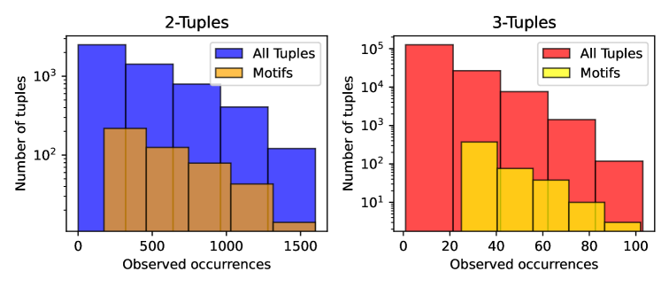
Figure S1: Distributions of the observed occurrences of unique tuples and motifs (i.e., significant tuples) in an artificial symbolic sequence created with our algorithm, for $2$-tuples (left) and $3$-tuples (right). These distributions refers to an artificial symbolic series created using an alphabet of $100$ symbols (plus the empty-space) and the following parameters: $n_{2}=478$, $n_{3}=499$ (starting from 500 randomly created 2-motifs and 500 3-motifs, with duplicates subsequently removed), $r_{2}=175$, $r_{3}=25$, $r_{ns}=10$, and $\gamma=-1$.

When tested on artificial sequences, our method shows comparable performance for both ordered and unordered motifs. Therefore, in the main manuscript and in the supplemental material, we report results only for the unordered case.

Fig. S1 shows an example of the distribution of the number of occurrences of $2$- and $3$-tuples, along with the distribution of significant tuples (motifs) of the corresponding sizes, resulting from a realization of the algorithm for artificial symbolic sequences (unordered case).

In this example, we generated a sequence starting from an alphabet of $100$ symbols (plus the empty-space) and using the following parameters: $n_{2}=478$, $n_{3}=499$ (starting from 500 randomly created 2-motifs and 500 3-motifs, with duplicates subsequently removed), $r_{2}=175$, $r_{3}=25$, $r_{ns}=10$, and $\gamma=-1$.

Demonstration on artificial datasets

Here, we illustrate how our method works using a synthetic dataset.

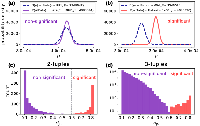
Figure S2: Testing the method on an artificial sequence with noise-to-signal ratio $r_{ns}=10$ and $\gamma=-1$ (linear rank-frequency distribution). (a–b) Comparison between prior $\Pi(p)$ and posterior $P(p\mid\text{Data})$ distributions for a non-significant tuple and a significant one (i.e., a motif), respectively. (c–d) Histogram of the number of $2$- and $3$-tuples as a function of the Jensen-Shannon distance $d_{\text{JS}}$. A logarithmic scale is used for the $y$-axis in panel (d) to improve readability, given the larger number of possible $3$-tuples compared to motifs.

In Fig. S2, we illustrate how our method, as described in the main manuscript, operates on an artificial symbolic sequence generated according to the procedure outlined in the previous section of the Supplemental Material. The result reported here (as all the other results on artificial series in the SM) are for the case of unordered tuples. In particular, this sequence was generated using an alphabet of $100$ symbols (plus the special empty-space symbol), and with the following parameters: $n_{2}=478$, $n_{3}=499$ (starting from 500 randomly created 2-motifs and 500 3-motifs, with duplicates subsequently removed), $r_{2}=175$, $r_{3}=25$, $r_{ns}=10$, and $\gamma=-1$. The resulting distribution of the number of occurrences of $2$- and $3$-tuples, along with the distribution of significant tuples (motifs) of the corresponding sizes, is shown in Fig. S1.

In Fig. S2(a–b), we compare the prior $\Pi(p)$ and posterior $P(p\mid\text{Data})$ distributions for a non-significant tuple and a significant one (i.e., a motif). The Jensen-Shannon distance is approximately $d_{\text{JS}}\simeq 0.1$ for the non-significant tuple and $d_{\text{JS}}\simeq 0.8$ for the motif. In panels (c) and (d), we report the histograms of the number of $2$- and $3$-tuples, respectively, as a function of the Jensen-Shannon distance $d_{\text{JS}}$ between prior and posterior distributions (i.e., the BJS-score, as defined in the main manuscript). In both cases, we observe that non-significant and significant tuples follow two distinct distributions: the former peaks around $\sim 0.1^{-}$, while the latter peaks at $\sim 0.8^{+}$. Here, we choose a hard significance threshold $\text{BJS}^{\text{thr}}=0.6$, meaning that tuples with a BJS-score exceeding this threshold are classified as significant.

In Fig. S3, we show the confusion matrices and performance metrics for the classification of $2$- and $3$-motifs, respectively, averaged over $100$ independent realizations of the artificial sequence. These $100$ artificial sequences contain on average $476\pm 4$ and $499\pm 1$ unique $2$- and $3$-motifs, respectively (we created $500$ of each, and then removed the duplicates). Our method demonstrates excellent classification performance in this task, as shown by the confusion matrices and the evaluation metrics—precision, recall, accuracy, and F1 score. We recall, that precision, recall, accuracy and F1 score are defined in terms of the confusion matrix entrances, as follow [47]:

Precision $$=\frac{TP}{TP+FP}$$ (S2)

Recall $$=\frac{TP}{TP+FN}$$ (S3)

Accuracy $$=\frac{TP+TN}{TP+TN+FP+FN}$$ (S4)

F1 $$=\frac{2\cdot\text{Precision}\cdot\text{Recall}}{\text{Precision}+\text{Recall}}=\frac{2TP}{2TP+FP+FN}$$ (S5)

where $TP$ is the number of true positive, $FP$ false positive, $TN$ true negative and $FN$ false negative.

For comparison, we report in Fig. S3(c-d) also the performance metrics for a standard measure of statistical significance and anomalies of an observation, namely the z-score (see the “z-score computation” section of the SM) with a threshold of significance $z^{\text{thr}}=3$ (i.e., considering as significant the tuples whose observed frequency falls outside $3$ standard deviations from the expected frequency). We observe that our method based on the BJS-score outperforms the z-score in terms of precision, accuracy, and overall performance (measured by the F1 score). This is especially true for the case of $3$-tuples, where the z-score finds many false positive, causing a dramatic degradation of performances. For example, we observe that the the F1 score for the classification of 2 and 3 motifs being respectively $\sim 1$ and $\sim 0.9$, while the F1 score for a classification based on the z-score is $\sim 0.6$ for the $2$-motifs and close to $\sim 0$ for the $3$-motifs.

In the next section of the Supplemental Material, we report the Receiver Operating Characteristic (ROC) and Precision-Recall (PR) curves for motif identification using both the BJS- and $z$-scores, on sequences with different noise distributions (i.e., different values of $\gamma$). These results demonstrate the robustness and generality of our findings, which hold independently of the specific threshold values and the rank-frequency distribution of symbols in the sequence.

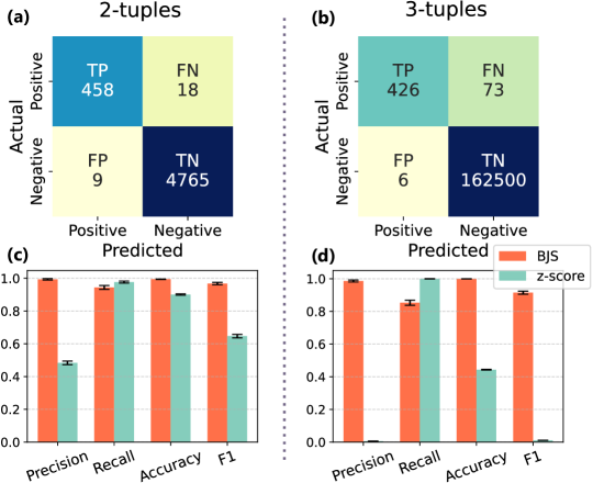
Figure S3: Confusion matrices for the BJS-score in the classification of $2$-tuples (a) and $3$-tuples (b) in artificial data, using a significance threshold of $\text{BJS}^{\text{thr}}=0.6$. (c,d) Bar plots showing the corresponding performance metrics of the BJS-score compared to those of the z-score, computed on the same data with a threshold of $z^{\text{thr}}=3$. Our method, based on the BJS-score, consistently outperforms the z-score, particularly in the detection of higher-order motifs.

Impact of symbols distribution and noise levels

We tested the impact of the symbol distribution and noise level on the method’s performance by using artificial symbolic sequences with varying values of $\gamma$, the exponent of the rank-frequency distribution $r(f)\sim f^{-\gamma}$. To isolate the effect of $\gamma$, all other parameters in the generation of the artificial sequences were kept fixed. As in the analysis of the Receiver Operating Characteristic (ROC) and Precision-Recall (PR) curves [47] presented in the main manuscript, we generated symbolic sequences using an alphabet of $100$ symbols, with $n_{2}=50$ 2-motifs and $n_{3}=50$ 3-motifs. Each motif was repeated $r_{2}=10$ and $r_{3}=5$ times, respectively. For each value of $\gamma$, we generated symbolic sequences with various noise levels. Specifically, we tested the performance under high noise conditions, with noise-to-signal ratios $r_{ns}\in\{5,10,25,50,100\}$. Differently from the main manuscript, here we report the performance of 2-motif and 3-motif recognition separately.

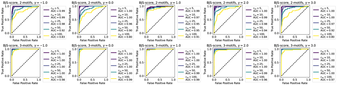
Figure S4: ROC curves showing the classification performance of the BJS-score for $2$-motifs (top panels) and $3$-motifs (bottom panels), across different symbol distributions (i.e., varying values of $\gamma$) and different noise-to-signal ratios $r_{ns}$. For each value of $r_{ns}$, the corresponding Area Under the Curve (AUC) is reported in the legend.

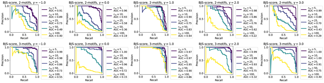
Figure S5: PR curve showing the classification performance of the BJS-score for $2$-motifs (top panels) and $3$-motifs (bottom panels), across different symbol distributions (i.e., varying values of $\gamma$) and different noise-to-signal ratios $r_{ns}$. For each value of $r_{ns}$, the corresponding Area Under the Curve (AUC) is reported in the legend.

In Fig. S4 and Fig. S5, we report the ROC and PR curves, respectively, for different values of $\gamma$, showing the classification performance of the BJS-score for $2$-motifs (top panels) and $3$-motifs (bottom panels). Given the class imbalance in our datasets (i.e., true motifs are rare compared to noise), the PR curves provide a more informative assessment of method performance than the ROC curves. For comparison, in Fig. S6 and Fig. S7, we report the ROC and PR curves corresponding to the classification performance of the $z$-score on the same datasets.

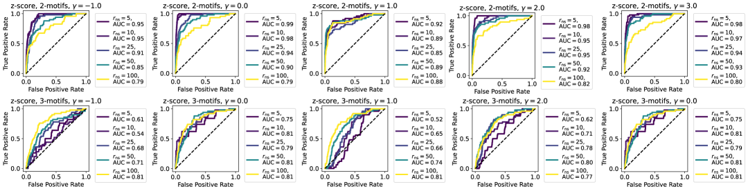
Figure S6: ROC curves showing the classification performance of the $z$-score for $2$-motifs (top panels) and $3$-motifs (bottom panels), across different symbol distributions (i.e., varying values of $\gamma$) and different noise-to-signal ratios $r_{ns}$. For each value of $r_{ns}$, the corresponding Area Under the Curve (AUC) is reported in the legend.

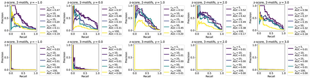
Figure S7: PR curve showing the classification performance of the $z$-score for $2$-motifs (top panels) and $3$-motifs (bottom panels), across different symbol distributions (i.e., varying values of $\gamma$) and different noise-to-signal ratios $r_{ns}$. For each value of $r_{ns}$, the corresponding Area Under the Curve (AUC) is reported in the legend.

From the curves and the corresponding Area Under the Curve (AUC) values [47], we observe that the BJS-score consistently demonstrates strong performance across all tested values of $\gamma$, with only a few exceptions occurring at extreme noise levels (i.e., for $r_{ns}\geq 25$). In all scenarios considered, the BJS-score clearly outperforms the $z$-score.

Choosing the threshold $\text{BJS}^{\text{thr}}(l)$

The choice of a significance hard threshold $\text{BJS}^{\text{thr}}(l)$ is inherently arbitrary. However, we outline below some rules of thumb and methodologies that can serve as useful guides for selecting a meaningful threshold.

From our analysis of ROC and PR curves on artificial sequences, we found that across all tested noise distributions (corresponding to several values of $\gamma$), the optimal $\text{BJS}^{\text{thr}}(l)$—that is, the value maximizing the F1 score—consistently falls between $0.5$ and $0.7$, for both $l=2$ and $l=3$. This provides a practical rule of thumb: this range is typically a good starting point for exploring threshold values and often yields good performance. This threshold also has a natural interpretation. The $\text{BJS}(\bm{s})$ measures the distance between prior and posterior distributions and takes values in the interval $[0,1]$, where $0$ indicates identical distributions and $1$ indicates completely different ones. Hence, a threshold above the midpoint $0.5$ intuitively corresponds to distributions that are more different than similar.

A more data-driven approach to selecting a meaningful $\text{BJS}^{\text{thr}}(l)$ for a specific dataset is as follows. Given a symbolic sequence, we create a randomized version by shuffling its symbols. We then compute the BJS-score for all tuples in this randomized sequence and compare these scores to those computed from the original sequence. One possible criterion is to take the maximum BJS-score obtained from the randomized sequence as a reference threshold: $\text{BJS}^{\text{thr}}(l)=\text{BJS}(\mathbf{s})$ for $|\mathbf{s}|=l$. In this way a tuple of lenght $l$ in the original sequence would be considered significant only if its BJS-score exceeds this value.

To account for fluctuations due to randomness, this procedure should be repeated across multiple independent re-shuffling processes, to obtain a robust statistic. However, for long sequences with many distinct symbols, this may require extremely long computational time, becoming impractical.

We tested this method on artificial sequences generated with different values of $\gamma$, and found that, although the threshold estimated using this procedure in general does not perfectly match the optimal $\text{BJS}^{\text{thr}}(l)$ (i.e., the one maximizing the F1 score), the typical range of both estimated and optimal thresholds is very similar—approximately between $0.5$ and $0.7$—thus confirming the reliability of this interval as a reasonable default choice.

z-score computation

The z-score of a $l$-tuple $\bm{s}$ is defined as follow:

$$\text{z-score}(\bm{s})=\frac{p_{\text{obs}}(\bm{s})-p_{\text{exp}}(\bm{s})}{\text{std}_{\text{exp}}(\bm{s})}$$ (S6)

where $p_{\text{exp}}(\bm{s})$ is the expected probability for observing $\bm{s}$ taking into account the effect of lower-order correlations coming from tuples of length smaller than $l$ [43], defined in the main manuscript. For the ordered case we have:

$$p_{\text{exp}}(\bm{s}=s_{1},s_{2}) =p_{\text{obs}}(s_{1})p_{\text{obs}}(s_{2})$$ (S7)

and:

$$p_{\text{exp}}(\bm{s}=s_{1},\dots,s_{l}) =\frac{p_{\text{obs}}(s_{1},\dots,s_{l-1})p_{\text{obs}}(s_{2},\dots,s_{l})}{p_{\text{obs}}(s_{2},\dots,s_{l-1})}$$ (S8)

for $l>2$. We recall from the manuscript, that the observed probability of $\bm{s}$ is computed as:

$$p_{\text{obs}}(\bm{s})=\frac{n_{\text{obs}}(\bm{s})}{S-l+1}$$ (S9)

where $n_{\text{obs}}(\bm{s})$ represents the number of occurrences of $\bm{s}$ in the sequence of length $S$ and $S-l+1$ is the total number of $l$-tuples. For the application to the case of unordered tuples, all we have to do is to sum the results for the ordered case over $S_{p}(\bm{s})$, the set of unique permutations $\bm{\sigma}$ of the ordered tuple $\bm{s}=s_{1},\dots,s_{l}$, obtaining:

$$p_{\text{exp}}^{\text{und}}(\bm{s})=\sum_{\bm{\sigma}\in S_{p}(\bm{s})}p_{\text{exp}}(\bm{\sigma})$$ (S10)

and

$$n_{\text{obs}}^{\text{und}}(\bm{s})=\sum_{\bm{\sigma}\in S_{p}(\bm{s})}n_{\text{obs}}(\bm{\sigma})$$ (S11)

In order to estimate the standard deviation $\text{std}_{\text{exp}}(\bm{s})$, we partition the original sequence in $m$ successive sub-sequences (namely, batches) of equal length. In each batch $i$ we compute $p_{\text{exp}}^{(i)}(\bm{s})$ and then we compute the standard deviation of $\bm{s}$ as:

$$\text{std}_{\text{exp}}(\bm{s})\approx\sqrt{\frac{\langle p_{\text{exp}}^{(i)}(\bm{s})^{2}\rangle-\langle p_{\text{exp}}^{(i)}(\bm{s})\rangle^{2}}{m-1}}$$ (S12)

where $\langle\cdot\rangle$ is the average over the $m$ batches. For our results, we partitioned the original sequence in $m=20$ batches.

Real-world data

For each dataset we selected a time bin $\Delta t$ commensurate with the resolution of the corresponding time series. For the brain data, we used $\Delta t=0.0015$ s, which corresponds to the neuronal refractory period—the typical time required for a neuron to become re-excitable after firing a spike. This choice was made to prevent the repetition of the same neuron within a single tuple, thereby avoiding self-loops or autocorrelations in neuronal activity. We verified that the results remain consistent across a wide range of $\Delta t$ values. In particular, for the datasets we analyzed, using $\Delta t=0.015$ s and $\Delta t=0.0015$ s, the overlap between significant hyperedges with a BJS-score $\geq 0.6$ is approximately $95\%$ for $2$-motifs and $85\%$ for $3$-motifs (relative to the smaller set of hyperedges), while the Jaccard similarity is around $94\%$ for $2$-motifs and $76\%$ for $3$-motifs. Further increasing $\Delta t$ leaves the results essentially unchanged, as for $\Delta t=0.015$ s the symbolic sequence already contains few to no space characters. Conversely, decreasing $\Delta t$ significantly below $0.0015$s begins to break the symbolic sequence, as the number of space characters becomes very large, resulting in many isolated spikes. Nonetheless, even at $\Delta t=0.0005$ s, when compared to $\Delta t=0.0015$ s, the overlap relative to the smaller set of hyperedges remains high: approximately $99\%$ for $2$-motifs and $60\%$ for $3$-motifs. The corresponding Jaccard similarity in this case is about $65\%$ for $2$-motifs and $45\%$ for $3$-motifs.

For the stock prices and email exchange time series, we instead used $\Delta t=1$ day, corresponding to the time resolution of the stock price data. Given the temporal resolution of these two datasets, we verified that the choice of $\Delta t$ plays only a marginal role: for essentially any reasonable value of the time window, the resulting symbolic sequences contain very few space characters. Although $\Delta t$ does not appear to have a significant impact for these specific datasets, this may not hold true for other types of data. In general, one should assess the influence of different $\Delta t$ values on the identification of motifs.

Data set	$N$	$E_{2}$	$E_{3}$	$\text{BJS}^{\text{thr}}$
Brain 1 activity (micro-scale)	346	3483	294	0.7
Brain 1 activity (micro-scale)	346	4546	794	0.6
Brain 1 activity (macro-scale)	15	38	115	0.7
Brain 1 activity (macro-scale)	15	42	130	0.6
Brain 2 activity (micro-scale)	361	3369	127	0.7
Brain 2 activity (micro-scale)	361	4572	491	0.6
Brain 2 activity (macro-scale)	18	56	146	0.7
Brain 2 activity (macro-scale)	18	61	187	0.6
Brain 3 activity (micro-scale)	392	3456	93	0.7
Brain 3 activity (micro-scale)	392	4737	484	0.6
Brain 3 activity (macro-scale)	18	57	166	0.7
Brain 3 activity (macro-scale)	18	60	201	0.6
Stock price changes (unsigned)	24	15	3	0.6
Stock price changes (signed)	48	70	0	0.6
Email exchanges	143	164	6	0.6

Table S1: Basic properties of the unweighted hypergraphs obtained from multivariate time-series, respectively from single-cell neuronal activity [48], financial stocks [49, 50], and email exchanges [52]. Values of $\text{BJS}^{\text{thr}}=0.6,0.7$ have been adopted to threshold the weighted hypergraphs. A larger threshold means that fewer hyperedges on average satisfy the condition $\text{BJS}^{\text{thr}}\leq\text{BJS}(\bm{s})$, resulting in more sparse hypergraphs (i.e., with less hyperedges). For the stocks and the emails network we show the results ony for $\text{BJS}^{\text{thr}}=0.6$, as adopting a threshold of $0.7$ results in no higher-order hyperedges.

Brain data.

We analyzed publicly available time series of neural activity with single-neuron resolution, provided by the Allen Institute. These datasets consist of multiple recording sessions performed on mice engaged in a visual task. For each mouse, approximately $500$ individual neurons were recorded during each session using Neuropixels technology. After filtering out neurons based on quality metrics—specifically retaining only those with an inter-spike interval (ISI) violation fraction $\text{isi}\leq 0.1$ and a signal-to-noise ratio $\text{snr}\geq 1.5$—we typically retained approximately $300$–$400$ neurons per session [48]. We applied our method to both the individual-neuron time series (and corresponding symbolic sequences), and an aggregated version in which neurons were grouped by their functional brain areas, as provided in the dataset metadata. Table S1 reports the number of nodes $N$, the number of $2$-motifs $E_{2}$, and the number of $3$-motifs $E_{3}$ in the unweighted hypergraphs obtained using significance thresholds $\text{BJS}^{\text{thr}}=0.6$ and $\text{BJS}^{\text{thr}}=0.7$. We present results for three different sessions of the “Brain Observatory” type [48], each corresponding to a different mouse. For each mouse, we analyzed all data available from the session, resulting in symbolic sequences of approximately $3\times 10^{7}$ symbols. In particular, “Brain 1” refers to session 773418906, “Brain 2” to session 791319847, and “Brain 3” to session 797828357 of the “Brain Observatory 1.1” dataset.

Stock market. We considered the historical time series publicly available through Yahoo finance, represented by the closure prices of $24$ stocks from NASDAQ Stock Market and New York Stock Exchange over $30$ years, from 1994 to 2024 [49, 50]. In particular, we selected $3$ stocks from $8$ different categories:

• technology:

  • Apple Inc. (AAPL)

  • Microsoft Corporation (MSFT)

  • International Business Machines Corporation (IBM)

• chemicals:

  • Dow Inc. (DOW)

  • LyondellBasell Industries N.V. (LYB)

  • DuPont de Nemours, Inc. (DD)

• banking:

  • JPMorgan Chase & Co. (JPM)

  • Bank of America Corporation (BAC)

  • Citigroup Inc. (C)

• entertainment:

  • The Walt Disney Company (DIS)

  • Comcast Corporation (CMCSA)

  • Sony Group Corporation (SONY)

• food and beverage:

  • the Coca-Cola Company (KO)

  • PepsiCo, Inc. (PEP)

  • General Mills, Inc. (GIS)

• pharmaceutical:

  • Pfizer Inc. (PFE)

  • Merck & Co., Inc. (MRK)

  • Johnson & Johnson (JNJ)

• energy:

  • Exxon Mobil Corporation (XOM)

  • Chevron Corporation (CVX)

  • ConocoPhillips (COP)

• consumer goods:

  • The Procter & Gamble Company (PG)

  • Colgate-Palmolive Company (CL)

  • Kimberly-Clark Corporation (KMB)

We first converted each time series of closing prices into a binary time series as follows: if the change in closing price of a stock exceeded $2\%$ compared to the previous closing price, we assigned a value of $1$ in the corresponding binary time series (representing a spike); otherwise, we assigned a $0$. We then applied the procedure described in the manuscript to map the binary multivariate time series of the $24$ stocks into a unique symbolic sequence of $25$ symbols (one for each stock, plus a special empty-space symbol). Given the daily timescale of this dataset, we inserted the empty symbol in the sequence whenever the time gap between two successive symbols exceeded $24$ hours. Finally, we extracted the $2$- and $3$-motifs from the symbolic sequence, as described in the manuscript. For this dataset, we repeated the entire procedure several times and observed minor fluctuations (on the order of $\pm 1$) in the number of motifs identified. This variability arises from the limited temporal resolution of the dataset, which causes many spikes (i.e., entries with value $1$ in the binary time series) to occur simultaneously. In such cases, to construct the symbolic time series, we must randomize the order of events that occur at the same time. This step introduces a degree of stochasticity in the mapping process, which in turn affects the final set of motifs. In all realizations of the procedure, we found that approximately $76\%$ of the pairwise motifs involved stocks belonging to the same category—an intuitively plausible result that supports the validity of our methodology. Regarding the $3$-motifs, our method identified as the most significant motifs the triplet (BAC, C, JPM), corresponding to the three banking stocks, and (COP, CVX, XOM), corresponding to the three energy stocks. Both motifs had a BJS-score of approximately $0.64\pm 0.02$.

We also considered the case of signed variations in stock prices by assigning each stock two distinct symbols: one representing a positive variation and the other a negative variation. Interestingly, in the case of signed changes, all the $2$-motifs—except one—involved stock price changes of the same sign ($36$ among symbols representing positive variations and $33$ among those representing negative variations). The only motif composed of symbols with opposite signs is (DOW$+$, DOW$-$), indicating that for the DOW stock, a variation in one direction is statistically associated with a subsequent correction in the opposite direction. In Table S1 we report the results relative to $\text{BJS}^{\text{thr}}=0.6$.

Email exchange. We constructed binary time series from the Enron dataset of internal emails exchanged by the company’s employees [52]. Specifically, we set $x_{i}(t)=1$ at time $t$ if employee $i$ sent an email at that time, and considered only email exchanges within the company—that is, from one Enron employee to other Enron employees. A centrality analysis performed on the resulting unweighted hypergraph identified the most central nodes as key figures within the company. In particular, we measured betweenness, closeness, and eigenvector centrality for the network nodes [10, 11], consistently finding key figures in the com- pany (e.g., vice presidents and chief operating officers) among the top 10 nodes across all centrality measures. In Table S1, we report the results corresponding to the threshold $\text{BJS}^{\text{thr}}=0.6$.

References

- Axelrod and Hamilton [1981] R. Axelrod and W. D. Hamilton, Science 211, 1390 (1981).
- Nowak and Highfield [2012] M. A. Nowak and R. Highfield, SuperCooperators: altruism, evolution, and why we need each other to succeed, 1st ed. (Free Press, New York, NY, 2012).
- Pastor-Satorras et al. [2015] R. Pastor-Satorras, C. Castellano, P. Van Mieghem, and A. Vespignani, Rev. Mod. Phys. 87, 925 (2015).
- Strogatz and Stewart [1993] S. Strogatz and I. Stewart, Scientific American 269, 102 (1993).
- Dehaene et al. [1998] S. Dehaene, M. Kerszberg, and J.-P. Changeux, Proceedings of the National Academy of Sciences 95, 14529 (1998).
- Strogatz [2001] S. H. Strogatz, Nature 410, 268 (2001).
- Boccaletti et al. [2006] S. Boccaletti, V. Latora, Y. Moreno, M. Chavez, and D. Hwang, Phys. Rep. 424, 175 (2006).
- De Vico Fallani et al. [2014] F. De Vico Fallani, J. Richiardi, M. Chavez, and S. Achard, Philosophical Transactions of the Royal Society B: Biological Sciences 369, 20130521 (2014).
- Chiarion et al. [2023] G. Chiarion, L. Sparacino, Y. Antonacci, L. Faes, and L. Mesin, Bioengineering 10, 10.3390/bioengineering10030372 (2023).
- Newman [2010] M. Newman, Networks (Oxford University Press, 2010).
- Latora et al. [2017] V. Latora, V. Nicosia, and G. Russo, Complex networks: principles, methods and applications, 1st ed. (Cambridge University Press, 2017).
- Cimini et al. [2019] G. Cimini, T. Squartini, F. Saracco, D. Garlaschelli, A. Gabrielli, and G. Caldarelli, Nature Reviews Physics 1, 58 (2019).
- Robiglio et al. [2025] T. Robiglio, M. Neri, D. Coppes, C. Agostinelli, F. Battiston, M. Lucas, and G. Petri, Phys. Rev. Lett. 134, 137401 (2025).
- Battiston et al. [2020] F. Battiston, G. Cencetti, I. Iacopini, V. Latora, M. Lucas, A. Patania, J.-G. Young, and G. Petri, Phys. Rep. 874, 1 (2020).
- Battiston et al. [2021] F. Battiston, E. Amico, A. Barrat, G. Bianconi, G. Ferraz de Arruda, B. Franceschiello, I. Iacopini, S. Kéfi, V. Latora, Y. Moreno, M. M. Murray, T. P. Peixoto, F. Vaccarino, and G. Petri, Nat. Phys. 17, 1093 (2021).
- Iacopini et al. [2019] I. Iacopini, G. Petri, A. Barrat, and V. Latora, Nat. Commun. 10, 2485 (2019).
- Alvarez-Rodriguez et al. [2021] U. Alvarez-Rodriguez, F. Battiston, G. F. de Arruda, Y. Moreno, M. Perc, and V. Latora, Nat. Hum. Behav 5, 586 (2021).
- Civilini et al. [2024] A. Civilini, O. Sadekar, F. Battiston, J. Gómez-Gardeñes, and V. Latora, Physical Review Letters 132, 167401 (2024).
- Yu et al. [2011] S. Yu, H. Yang, H. Nakahara, G. S. Santos, D. Nikolić, and D. Plenz, Journal of Neuroscience 31, 17514 (2011).
- Petri et al. [2014] G. Petri, P. Expert, F. Turkheimer, R. Carhart-Harris, D. Nutt, P. J. Hellyer, and F. Vaccarino, J. R. Soc. Interface 11, 20140873 (2014).
- Squartini and Garlaschelli [2017] T. Squartini and D. Garlaschelli, Maximum-Entropy Networks: Pattern Detection, Network Reconstruction and Graph Combinatorics, SpringerBriefs in Complexity (Springer, Cham, 2017).
- Squartini et al. [2018] T. Squartini, G. Caldarelli, G. Cimini, A. Gabrielli, and D. Garlaschelli, Physics Reports 757, 1 (2018).
- Chelaru et al. [2021] M. I. Chelaru, S. Eagleman, A. R. Andrei, R. Milton, N. Kharas, and V. Dragoi, Neuron 109, 3954 (2021), publisher: Elsevier.
- Santoro et al. [2024] A. Santoro, F. Battiston, M. Lucas, G. Petri, and E. Amico, Nat. Commun. 15, 10244 (2024).
- Yu et al. [2006] D. Yu, M. Righero, and L. Kocarev, Phys. Rev. Lett. 97, 188701 (2006).
- Timme [2007] M. Timme, Phys. Rev. Lett. 98, 224101 (2007).
- Garlaschelli and Loffredo [2008] D. Garlaschelli and M. I. Loffredo, Phys. Rev. E 78, 015101 (2008).
- Han et al. [2015] X. Han, Z. Shen, W.-X. Wang, and Z. Di, Phys. Rev. Lett. 114, 028701 (2015).
- Brugere et al. [2018] I. Brugere, B. Gallagher, and T. Y. Berger-Wolf, ACM Comput. Surv. 51, 10.1145/3154524 (2018).
- Musciotto et al. [2021] F. Musciotto, F. Battiston, and R. N. Mantegna, Communications Physics 4, 218 (2021).
- Young et al. [2021] J.-G. Young, G. Petri, and T. P. Peixoto, Communications Physics 4, 135 (2021).
- Lizotte et al. [2023] S. Lizotte, J.-G. Young, and A. Allard, Scientific Reports 13, 21364 (2023).
- Malizia et al. [2024] F. Malizia, A. Corso, L. V. Gambuzza, G. Russo, V. Latora, and M. Frasca, Nat. Commun. 15, 5184 (2024).
- Delabays et al. [2025] R. Delabays, G. De Pasquale, F. Dörfler, and Y. Zhang, Nat. Commun. 16, 2691 (2025).
- Santoro et al. [2023] A. Santoro, F. Battiston, G. Petri, and E. Amico, Nature Physics 19, 221 (2023).
- Varley et al. [2023] T. F. Varley, M. Pope, M. G. Puxeddu, J. Faskowitz, and O. Sporns, Proc. Natl. Acad. Sci. U.S.A. 120, e2300888120 (2023).
- Keogh et al. [2001] E. Keogh, K. Chakrabarti, M. Pazzani, and S. Mehrotra, Knowl. Inf. Syst. 3, 263 (2001).
- Lin et al. [2007] J. Lin, E. Keogh, L. Wei, and S. Lonardi, Data Mining and Knowledge Discovery 15, 107 (2007).
- Wang et al. [2022] H. Wang, C. Ma, H.-S. Chen, Y.-C. Lai, and H.-F. Zhang, Nature Communications 13, 3043 (2022).
- Newman [2005] M. Newman, Contemporary Physics 46, 323 (2005).
- Beck and Schögl [1993] C. Beck and F. Schögl, Thermodynamics of Chaotic Systems: An Introduction, Cambridge Nonlinear Science Series (Cambridge University Press, 1993).
- Daw et al. [2003] C. S. Daw, C. E. A. Finney, and E. R. Tracy, Review of Scientific Instruments 74, 915 (2003).
- Sinatra et al. [2010] R. Sinatra, D. Condorelli, and V. Latora, Phys. Rev. Lett. 105, 178702 (2010).
- Lin [1991] J. Lin, IEEE Trans. Inf. Theory 37, 145 (1991).
- Abbott et al. [2019] B. P. Abbott et al. (LIGO Scientific Collaboration and Virgo Collaboration), Phys. Rev. X 9, 031040 (2019).
- Pratten et al. [2020] G. Pratten, P. Schmidt, R. Buscicchio, and L. M. Thomas, Phys. Rev. Res. 2, 043096 (2020).
- Powers and Ailab [2011] D. Powers and Ailab, J. Mach. Learn. Technol 2, 2229 (2011).
- all [2019] Neuropixels Visual Coding, Tech. Rep. (Allen Brain Observatory, 2019).
- Yahoo Finance [2025] Yahoo Finance, Historical stock data (1994–2024) (2025).
- Aroussi [2025] R. Aroussi, yfinance: Yahoo! finance market data downloader, https://github.com/ranaroussi/yfinance (2025), used to download stock price data from 1994 to 2024.
- Bonanno et al. [2001] G. Bonanno, F. Lillo, and R. Mantegna, Quant. Finance 1, 96 (2001).
- Klimt and Yang [2004] B. Klimt and Y. Yang, in Machine Learning: ECML 2004, edited by J.-F. Boulicaut, F. Esposito, F. Giannotti, and D. Pedreschi (Springer Berlin Heidelberg, Berlin, Heidelberg, 2004) pp. 217–226.
- Tang et al. [2013] J. Tang, I. Leontiadis, S. Scellato, V. Nicosia, C. Mascolo, M. Musolesi, and V. Latora, Applications of temporal graph metrics to real-world networks, in Temporal Networks, edited by P. Holme and J. Saramäki (Springer Berlin Heidelberg, Berlin, Heidelberg, 2013) pp. 135–159.
- Theiler et al. [1992] J. Theiler, S. Eubank, A. Longtin, B. Galdrikian, and J. Doyne Farmer, Physica D: Nonlinear Phenomena 58, 77 (1992).