pySTARBURST99: The Next Generation of STARBURST99

Abstract

Starburst99  is a population synthesis code tailored to predict the integrated properties or observational characteristics of star-forming galaxies. Here we present an update to Starburst99  where we port the code to python, include new evolutionary tracks both rotating and non-rotating at a range of low metallicity environments. We complement these tracks with a corresponding grid of new synthetic SEDs. Additionally we include both evolutionary and spectral models of stars up to 300-500$\rm M_{\odot}$. Synthesis models made with the python version of the code and new input stellar models are labelled pyStarburst99. We make new predictions for many properties, such as ionising flux, SED, bolometric luminosity, wind power, hydrogen line equivalent widths and the UV $\beta$-slope. These properties are all assessed over wider coverage in metallicity, mass and resolution than in previous versions of Starburst99. A notable finding from these updates is an increase in H I ionising flux of 0.3 dex in the first 2Myr when increasing the upper mass limit from 120 to 300$\rm M_{\odot}$. Changing metallicity has little impact on H I in the first 2Myr (range of 0.015 dex from $Z=0.02$ to $0.0$) but lower metallicities have higher H I by 1 dex (comparing $Z=0.02$ to $0.0004$) at later times, with $Z=0.0$ having even higher H I at later times. Rotating models have significantly higher H I than their equivalent non-rotating models at any time after 2Myr. Similar trends are found for He I and He II, bolometric luminosity and wind momentum, with more complex relations found for hydrogen line equivalent widths and UV $\beta$-slopes.

1 Introduction

Young stellar populations are characterised by the intense UV flux from the most massive stars (e.g. Leitherer, 2020). Therefore, key observational diagnostics in star-forming galaxies come from the extended atmospheres of stars which are hot and luminous enough to drive stellar winds, through radiation-pressure acting on metal ions in the photosphere. Beside being responsible for a significant amount of the ionising flux produced in starburst galaxies, due to their intrinsically hot temperatures, the strong winds lead to a significant environmental enrichment of momentum, energy and heavy elements (e.g. Geen et al., 2023). With this in mind, synthetic stellar populations are an essential tool, to make predictions of both directly measurable and only inferrable integrated properties of galaxies with ongoing star formation, both as probes of the stellar content and as a fundamental element in the assessment of nebular properties.

However, synthetic stellar populations crucially depend on the capabilities of the underlying stellar models they are built upon (e.g. Conroy et al., 2009). Consequently, the inherent uncertainties in the composition of the stellar population or the evolutionary pathways directly limit the predictive power of the population models. While fundamental questions about the physical processes in massive stars remain, population synthesis models need to keep up with the progress made in the field, for example related to mass-loss, angular momentum transport, and the impact of stellar interactions in binary and multiple systems (see e.g. Langer, 2012; Eldridge & Stanway, 2022; Marchant & Bodensteiner, 2024). Moreover, there are further fundamental limitations imposed by the scope of available grids of underlying stellar models. In particular we focus on two quantities, the metallicity and the upper mass limit of the IMF, which are key to understand unresolved populations throughout the Universe.

The initial stellar mass is the primary driver of the evolutionary pathway. Massive stars stars lose a significant fraction of their mass through their stellar winds, which are inherently metallicity dependent, therefore it is crucial that models at various metallicities are available. Especially given our increased understanding of local populations with sub-solar metallicity, e.g., through large observing programmes like ULLYSES (Roman-Duval et al., 2020) and its optical complement XShootU (Vink et al., 2023) on the level of individual stars as well as CLASSY (Berg et al., 2022) and the rapidly expanding list of observed galaxies in the early Universe with JWST on the level of star-forming galaxies. There are a wide range of available stellar evolutionary models with massive stars (bpass, Eldridge et al., 2017; cigale, Boquien et al., 2019; fsps, Conroy & Gunn, 2010; galev, Kotulla et al., 2009; Galaxev, Bruzual & Charlot, 2003; Plat et al., 2019; Galsevn, Lecroq et al., 2024; miles, Vazdekis et al., 2016; Pegase, Le Borgne et al., 2004; Slug, Krumholz et al., 2015; HR-pyPopStar, Millán-Irigoyen et al., 2021; Starburst99, Leitherer et al., 1999, 2014). Pegase  and miles  are based on empirical spectral libraries, and galev  uses the Lejeune et al. (1997) theoretical library. The other codes (bpass, cigale, fsps, Galaxev, Slug, Starburst99) are more tailored for spectral synthesis including massive stars. All of these codes utilise WMbasic  (Pauldrach et al., 2001) atmosphere models for OB stars to produce synthetic spectra, apart from HR-pyPopStar  which implements the powr  model grid (Hainich et al., 2019) covering $Z=0.014,0.006,0.002$. The individual stellar parameters in each WMbasic  grid vary but the metallicites are the same, with the range $Z=0.04,0.02,0.008,0.004,0.001$ in cigale, Galaxev, Slug  and Starburst99 . bpass  adds models at $Z=0.006$ and $0.002$ and fsps  adds models at $Z=0.0001,0.003,0.01,0.014,0.03$. However, the various stellar evolutionary tracks (discussed further in Sect. 2.1) used by bpass, cigale, Galaxev, Slug, Starburst99), offer many more metallicites (see e.g. Table 10 in Sánchez et al., 2022, Table 1 in Eldridge et al., 2017 and Table 1 in Leitherer et al., 2014). This means that the majority of population synthesis models rely on interpolation in metallicity to produce spectra, especially at low metallicity.

A growing area of interest is the impact of stars with (initial) masses above 100 $M_{\odot{}}$, also known as very massive stars (VMS). Such stars are exceedingly rare (from an IMF perspective) but highly impactful, and their presence in stellar populations is inferred in a number of observations of distant galaxies (Senchyna et al., 2021; Meštrić et al., 2023; Upadhyaya et al., 2024). Resolved VMS have been directly detected in Galactic clusters (NGC3603; Schnurr et al., 2008; Crowther et al., 2010, Arches; Figer et al., 2002; Najarro et al., 2004; Martins et al., 2008; Lohr et al., 2018) with the most massive stars found in the LMC cluster R136 (see, e.g., Crowther et al., 2010, 2016; Bestenlehner et al., 2020; Kalari et al., 2022; Brands et al., 2022). Tentative detections of these objects in relatively nearby star-forming regions has become increasingly common (e.g., Wofford et al., 2014; Smith et al., 2016; Wofford et al., 2023; Smith et al., 2023). This could enable some verification of VMS predictions. Coupling this progress with the argument that VMS form more readily in low metallicity environments; the motivation to properly account for VMS in stellar population models grows as they help inform our understanding of the earliest generations of stars. Some population synthesis codes have taken steps to account for the presence of VMS. The Galaxev  and BPASS codes now include stellar evolutionary predictions for stars up to initial masses of 300 $M_{\odot{}}$, albeit without dedicated updates to the VMS spectral libraries, although Galaxev do include PoWR spectra for WNL stars as a close proxy to the spectra of VMS. New studies are building upon these evolutionary models with tailored complementary stellar atmosphere models in attempts to reproduce galactic spectra (Martins & Palacios, 2022; Schaerer et al., 2024; Martins et al., 2025). There have also been empirical approaches with works such as Crowther & Castro (2024) creating composite stellar populations using dedicated UV spectroscopy as well as the ULLYSES library of massive star spectra to recreate composite observations of R136, which can inform our interpretation of spectra of highly star-forming regions at larger distances. An additional observational complication is the difficulty in distinguishing between VMS and Wolf-Rayet (WR) stars in composite rest-frame UV spectra (Martins et al., 2023; Rivera-Thorsen et al., 2024; Berg et al., 2024), with these two populations of stars having a number of similar spectral signatures while providing significantly different contributions to integrated population properties.

Significant progress has been made in the field of stellar evolution in the past decade. With respect to Starburst99, of particular interest is the tremendous extension of the Genec suite of stellar tracks as the underlying mapping of stellar evolution in the population synthesis modelling. Available Genec evolutionary models for initial masses from from 1 to 120 $M_{\odot}$ now cover a considerable range of metallicities, representing the conditions in a wide selection of environments, from the metal enhanced Galactic Nucleus through solar composition to the metal-poor Large and Small Magellanic Clouds, as well as very low metallicity galaxies such as IZw18 and completely metal-free regions, which would harbour Pop III objects. The Genec grids have further been extended in the mass domain with models available for initial masses up to 500 $M_{\odot}$ at $Z=0.02$ and $0.014$, and up to 300 $M_{\odot}$ at $Z=0.006$ and $0.0$. Following the success found in better reproducing the distribution of stars across the HRD by including a treatment of rotation in previous evolutionary grids (Levesque et al., 2012; Leitherer et al., 2014), models including rotation are available for all the aforementioned Genec extensions as well. Yet, to fully realise the predictive power of new evolutionary model grids, they must be paired with complementary synthetic model spectra from stellar atmosphere models which are representative of their parameter space coverage. There has also been substantial progress in the development of NLTE atmosphere models since the release of the commonly used WMbasic grid (in codes such as cmfgen  (Hillier & Miller, 1998), powr  (Gräfener et al., 2002; Sander et al., 2015) and Fastwind  Santolaya-Rey et al., 1997; Puls et al., 2005, discussed further in Sect. 2.2), providing a range of options to update stellar atmospheres for spectral synthesis modelling of starburst populations.

This tremendous progress in the modelling of stellar evolution and atmospheres has yet to be combined and implemented in a population synthesis framework to explain unresolved stellar populations. In this work, we aim to utilise these advancements in stellar models to update the capabilities of the population synthesis code Starburst99, with a focus on the impact of metallicity and upper mass limit. We present a new version of Starburst99, in which we implement the latest generation of Genec releases (covering $Z=0.02$, $0.014$, $0.006$, $0.002$, $0.0004$ and $0.0$) with rotation and include VMS (500 $\rm M_{\odot}$ at 0.014 and 300 $\rm M_{\odot}$ at lower metallicity), along with a new grid of complementary synthetic spectra from Fastwind.

Sect. 2 discusses the implementation of the aforementioned stellar evolutionary models in Starburst99, along with new tailored stellar atmosphere models produced to complement the tracks and our efforts to translate the Starburst99  code from Fortran  to python. Sect. 3 makes new predictions on a few key properties of the composite populations, such as their spectral energy distribution (SED), especially the ionising spectrum, as well as wind power and UV slope. Finally, we discuss the impact of these new predictions and highlight upcoming future work in Sect. 4.

2 Updates

In this section, we will outline the major updates made to Starburst99  focusing on the developments made in three key areas: (i) the included evolutionary models, (ii) the applied stellar atmosphere models, and (iii) the framework of the software itself being ported to python from Fortran.

2.1 Stellar evolution

Stellar evolutionary predictions have developed significantly in the past decade, with various libraries available which focus on massive stars produced with different codes (and each tailored to a specific parameter space). These include MIST (MESA models; Paxton et al., 2013; Dotter, 2016; Choi et al., 2016) and BONN tracks tailored to the Magellanic Clouds and their extension through BoOST (Brott et al., 2011; Köhler et al., 2015; Szécsi et al., 2022), both of which offer a wide range of masses and metallicities for single star evolutionary scenarios and include rotation. Many other options are available for more specific purposes such as investigating post-MS binary evolution or very massive stars (Marchant et al., 2017; Stevenson et al., 2017; Pauli et al., 2022; Broekgaarden et al., 2021; Martins & Palacios, 2022; Sabhahit et al., 2022; Fragos et al., 2023). For those used in population spectral synthesis, PARSEC models in GALEXEV (Bruzual & Charlot, 2003; Chen et al., 2015) which have high sampling in rotation and are adapted for binaries with Galsevn, STARS including binaries for BPASS Eldridge & Tout, 2004; Eldridge et al., 2017, and the Genec  models in Starburst99  (Maeder & Meynet, 1994; Leitherer et al., 1999; Levesque et al., 2012; Leitherer et al., 2014; Ekström et al., 2012; Georgy et al., 2013). We also note that caution should be taken when comparing evolutionary tracks, as there may be differences in predictions for similar stars as discussed in e.g. Agrawal et al. (2021). For specific physical effects such as rotation, there can also be differences in implementation between codes (Nandal et al., 2024).

In principle, any or all of the aforementioned tracks could be incorporated within the framework of Starburst99. For the immediate purpose of this work to extend Starburst99 models to lower metallicity and higher mass, and the straight-forward comparison with the currently established Starburst99  models, we implement the Genec  evolutionary tracks (Ekström et al., 2012; Georgy et al., 2013; Groh et al., 2019; Eggenberger et al., 2021; Murphy et al., 2021; Yusof et al., 2022; Martinet et al., 2023). A further extension to allow data from different evolutionary codes to be processed is envisioned, but is beyond the scope of the current work.

The implementation of solar and SMC metallicity tracks, defined relative to the solar metallicity of $Z=0.014$ (Asplund et al., 2009), from Ekström et al. (2012) and Georgy et al. (2013) are described in Leitherer et al. (2014). We follow the same routine to include the LMC, IZw18 and Z=0 (Z0) tracks. The LMC and IZw18 tracks follow the same physical recipes as described in Ekström et al. (2012) and Georgy et al. (2013). The Vink et al. (2001) mass-loss rates are implemented on the main sequence (MS), de Jager et al. (1988) is used in the blue supergiant (BSG) phase, a combination of Sylvester et al. (1998) and van Loon et al. (1999) in the red supergiant (RSG) phase and either Nugis & Lamers (2000) or Gräfener & Hamann (2008) in the WR regime. Additionally, the correction factor from Maeder & Meynet (2000) is applied to the mass-loss rates in rotating models. The applied mass-loss descriptions are consistent within one set of tracks. Between different sets, there are only slight differences in mass-loss scaling with metallicity as $\dot{M}(Z)=(Z/Z_{\odot})^{\alpha}\dot{M}(Z_{\odot})$ (see Table 1). We discuss the mass-loss rates in the context of Starburst99  outputs further in Sect. 3.3. For the Z0 tracks, there is no mass loss unless the star reaches a critical rotation threshold, at which point an average mass-loss rate of $10^{-5}\rm M_{\odot}\,yr^{-1}$ is applied until the star passes back under the rotation threshold. This mass loss is invoked only for parts of the evolution in the most massive stellar models ($>85\rm M_{\odot}$). For stars with $M>40\rm M_{\odot}$, as described in Ekström et al. (2012) and Georgy et al. (2013), a density-scale based mixing length for including turbulent pressure and acoustic flux in the envelope is used. All grids offer two rotation options (non-rotating and an initial velocity of 40% critical rotation), and none include the effects of magnetic fields. Therefore the models are differentially rotating.

We also note that the mass ranges and sampling differ between some of the grids. Mainly there is a slight decrease in range and sampling below SMC metallicity and an increase in sampling in the MW grid. For tests of the impact of mass resolution in the MW, comparing isochrones generated with either 24 or 33 evolutionary tracks, we find that there is very little impact on the isochrones during the main sequence. There are changes at higher masses when the post-MS evolution is more sensitive to smaller changes in mass. There are therefore significant differences at times when WR stars are present in the population, likely due to the addition of a $50\rm M_{\odot}$ track which reduces interpolation distance between the $40\rm M_{\odot}$ and $60\rm M_{\odot}$ tracks. The impact of these additional tracks is discussed in Sect. 3.1.

Initial heavy element mixtures at all metallicites follow Ekström et al. (2012) and are tuned down, essentially meaning they are solar-scaled abundances. This may not be fully representative of the suggested regions as $\alpha$-element ratios may vary in low metallicity environments as evidenced in nearby low-Z star forming regions Bouret et al. (2015); Schösser et al. (2025) and galaxies close to Cosmic Noon and at high redshift Steidel et al. (2016); Cullen et al. (2021); Strom et al. (2022); Cameron et al. (2023); Welch et al. (2025). Recent works have begun to investigate and quantify the impact of non-solar abundance patterns on predictions of stellar populations Pietrinferni et al. (2021); Grasha et al. (2021); Byrne et al. (2025).

For the VMS models from Martinet et al. (2023), the input physics is the same as for other Genec  models, apart from an increase in overshooting to 20% of the pressure scale height at the Ledoux boundary and the inclusion of electron-positron pair production in the equation of state. The mass loss-metallicity scaling follows Georgy et al. (2013). We note the evolution models do not contain a general increase in mass-loss rate for VMS on the main sequence, which would be physically motivated by proximity to the Eddington limit (Gräfener & Hamann, 2008; Vink et al., 2011; Bestenlehner et al., 2014; Sabhahit et al., 2022). The initial masses added are 180, 250 and 300 $\rm M_{\odot}$ at MW, LMC and Z0. This means there are no VMS tracks to match the exact metallicities of the SMC or IZw18. There is further a $500\,\rm M_{\odot}$ non-rotating track at solar metallicity.

Table 1: Properties of the stellar evolutionary models.

Region	Ref	H	He	Z	$\alpha$	$\alpha$	$\alpha$	$\alpha$	M	M	No. tracks
					$\dot{M}_{\mathrm{O}}$	$\dot{M}_{\mathrm{BSG}}$	$\dot{M}_{\mathrm{WR}}$	$\dot{M}_{\mathrm{R(S)G}}$	$v_{r0}$	$v_{r4}$
GalC	Yus22	0.7064	0.2735	0.02	0.85	0.5	0.66	1	0.8-500	0.8-300	33
MW	Eks12	0.72	0.266	0.014	1	1	1	1	0.8-500	0.8-300	33
LMC	Egg21	0.738	0.256	0.006	0.7	0.7	0.7	1	0.8-300	0.8-300	24
SMC	Geo13	0.747	0.251	0.002	0.85	0.5	0.66	1	0.8-120	0.8-120	24
IZw18	Gro19	0.7507	0.2489	0.0004	0.85	0.5	0.66	1	1.7-120	0.8-120	17
Z0	Mur21	0.7516	0.2484	0.0	-	-	-	-	1.7-300	0.8-300	16
VMS	Mar23	0.7516	0.2484	0.00001	0.7	0.7	0.7	1	180-300	180-300	3

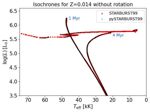
Figure 1: Isochrones computed with $Z=0.014$ Genec  tracks without rotation from 1-4 Myr. The tracks in red are produced with Starburst99  and the tracks in black are produced with pyStarburst99, showing good agreement between the two code versions.

2.2 Stellar spectral library

Two different synthetic spectral libraries for MS OB stars are used in Starburst99. The first is a grid of 33 models per metallicity, linearly sampled in effective temperature and surface gravity, which have large wavelength coverage ($90-16\times 10^{5}$Å) at relatively low (and wavelength dependent) resolution. These spectra are used to generate SEDs. The second is a set of 86 models per metallicity, with base stellar parameters tailored to the evolutionary tracks. These models are higher resolution UV spectra ($900-3000$Å) used to generate spectra with synthetic line profiles. Both of these libraries were produced with WMbasic. Other spectral libraries are available, e.g. for the post-MS, at optical wavelengths or from empirical spectra. The Starburst99  spectral libraries are discussed further in e.g Leitherer et al. (2010, 2014). To fully realise the impact of the new suite of evolutionary models we generate an entirely new grid of stellar atmosphere models with Fastwind  (Santolaya-Rey et al., 1997) to replace the current WMbasic  OB library and to fill gaps in the newly established parameter space. In this work we create models to replace only the low resolution synthetic spectral library used to produce SEDs, with plans to update the high resolution spectral library in a future work. Both WMbasic  and Fastwind  are designed for unified stellar atmosphere and wind modelling of hot (OBA) stars with steady-state, spherically symmetric radiatively driven winds in NLTE (non-local-thermodynamic-equilibirium). One unique aspect of WMbasic is the option to solve the hydrodynamical equations with a set of line force parameters to inherently obtain the mass-loss rate and velocity profile rather than using a prescription. For the WMbasic-models applied in Starburst99  Leitherer et al. (2010), the line force parameters were not iterated self-consistently, but pre-specified based on the metallicity-dependence for the wind-momentum luminosity relation derived by Kudritzki & Puls (2000). In the Fastwind models applied in this work, we instead use the common, numerically less costly approach to prescribe the hydrodynamic structure with a quasi-hydrostatic photosphere connected to a $\beta$-type velocity law. This is a standard treatment to create grids of synthetic stellar spectra (see, e.g., the recent method overview in Sander et al., 2024). Specifically, our calculated Fastwind models employ a smooth transition at 10% of the isothermal gas sound speed. This results in additional input parameters relating to the description of the stellar wind, the total mass-loss rate $\dot{M}$, the aforementioned $\beta$ and the terminal wind velocity $v_{\infty}$. We do not make use of the v11-branch of Fastwind (Puls et al., 2020) to compute the radiative transfer of all line transitions in the comoving frame (CMF), but instead use the CMF only for specified ’foreground’ elements while approximating the rest through an approximated line-blanketing formalism. This enables a substantial speed-up in computation time compared to other codes, such as cmfgen  or powr. Nonetheless, the new Fastwind models contain improvements in the implementation of physical processes such as line-blanketing and pressure broadening, as well as atomic data. An extensive comparison between WMbasic  and Fastwind  was made in Puls et al. (2005), finding generally very good agreement in the UV between the two codes with a few caveats in the wavelength range below 400Å. Since this comparison was made, there have been two full further releases of Fastwind, consisting of a number of important updates, such as the treatments of X-rays and wind clumping (Carneiro et al., 2016; Sundqvist & Puls, 2018). While these have a significant effect on individual line profiles, they should not have too much impact on the overall SED.

The current WMbasic  model grid consists of 33 models per metallicity, at 5 metallicites ($Z=0.001$, $0.004$, $0.008$, $0.02$, and $0.04$). We replicate the parameter space coverage with Fastwind, but adjust the input metallicities for consistency with the Genec  models ($Z=0.0$, $0.0004$, $0.002$, $0.006$, $0.014$ and $0.02$). Additionally, we extend the parameter space coverage to account for evolutionary predictions of VMS. This is achieved through a 33% increase in the size of the model grid, illustrated in Figure 2.

For this set of low-resolution stellar SEDs we do not include the effects of X-rays or wind clumping. Additionally we do not tailor mass-loss rates. All of these physical properties will need to be included to reproduce high resolution individual line profiles but have little impact on the overall SED.

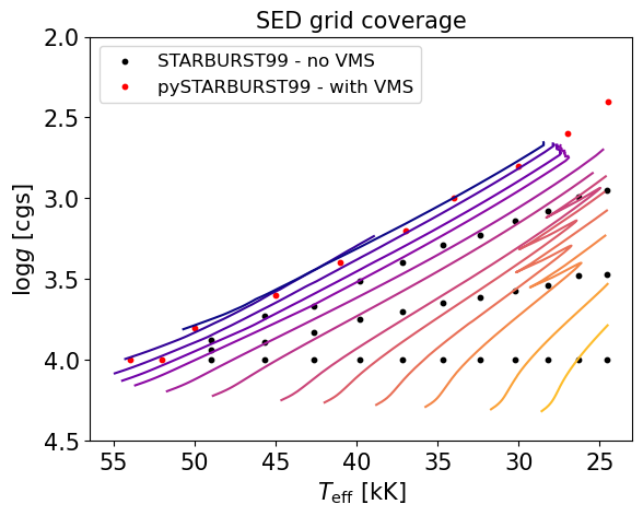
Figure 2: Example of grid coverage for SED predictions with extension for VMS at $Z=0.014$. Genec  evolutionary tracks are overplotted at regular intervals from 9-500$\rm M_{\odot}$. This coverage is available for all metallicities. A similar level of coverage is available at zero-metallicity where the tracks are much hotter than any others.

2.3 Python

In translating the code to python from Fortran, our primary goal is to increase the portability and usability of Starburst99. With the widespread use of python in the community we hope the new version will facilitate the use of pyStarburst99 with other astrophysical python packages and make the code more accessible. For the present work, we do not reproduce the full capabilities of Starburst99  but focus, for now, on a few key modules: spectral synthesis at low resolution in order to produce SEDs and the ability to make predictions on the ionising flux, wind power and $\beta$-slope. At the foundation of the framework of Starburst99  is the translation of stellar evolutionary tracks into stellar isochrones, in order to interpolate between tracks and make predictions at arbitrary resolution in mass within the range covered by the tracks. One of the often cited drawbacks for a python programme is the speed relative to Fortran, although much of this can be alleviated with the use of packages which act as wrappers around compiled code languages including Fortran and C, such as NumPy and SciPy. The bulk of the computational time occupied by Starburst99 is the isochrone synthesis. Thus, the computation time primarily scales with the resolution in mass of the isochrones, which in turn affects the speed of any dependent routines, i.e., higher resolution isochrones will be inherently more expensive in assigning synthetic spectra. To ensure similar runtimes we implement SciPy and NumPy functions for intensive computations in pyStarburst99. This results in typical pyStarburst99 runtimes ranging between 15 to 60 seconds, depending on the input options, which is comparable to Starburst99. In an attempt to further speed-up the code we also re-establish the resolution as a flexible input parameter and test which resolution is sufficient to produce statistically indistinguishable SEDs to make a recommendation for the input resolution in order to minimise computational load. For instance, it may be optimal to reduce resolution when running exploratory models or applying a flexible fitting routine and increase it when generating a grid or verifying a best-fit solution. Alternately, we introduce the option to increase the resolution within a specified mass range. However, as the interpolation is computed track-to-track, the specificity of the mass range is limited by the ZAMS mass sampling of the input evolutionary tracks. The interpolation scheme is the most tangible variation between Starburst99 and pyStarburst99 with Starburst99 implementing methods from numerical recipes (McCracken and Dorn) and pyStarburst99 using Scipy functions (based on Direckx). However this has fairly little impact on the results of the interpolation and production of isochrones, as shown in Fig. 1. For the resolution implemented as default, there is essentially no difference between Fortran  and the python versions.

We hope that the flexibility of the new language will make the code more portable and user-friendly, enabling more users to make predictions for starburst galaxies themselves and to tailor the code to their interests. However, to avoid blocking functionality of existing user-built frameworks, we also include the new range of metallicity in evolutionary tracks and spectral models in the standard Fortran  version of Starburst99, available on request or via the Starburst99 website (Starburst99), although we do not include VMS in the fortran version. The full functionalities of Starburst99  will be built into the python version over time and released alongside further improved builds. The current version of pyStarburst99 is available to download at GitHub (GitHub - pyStarburst99) or to run in browser with Colab (Colab - pyStarburst99). User feedback is encouraged by email to pystarburst99@gmail.com.

3 Results

3.1 Spectral energy distributions

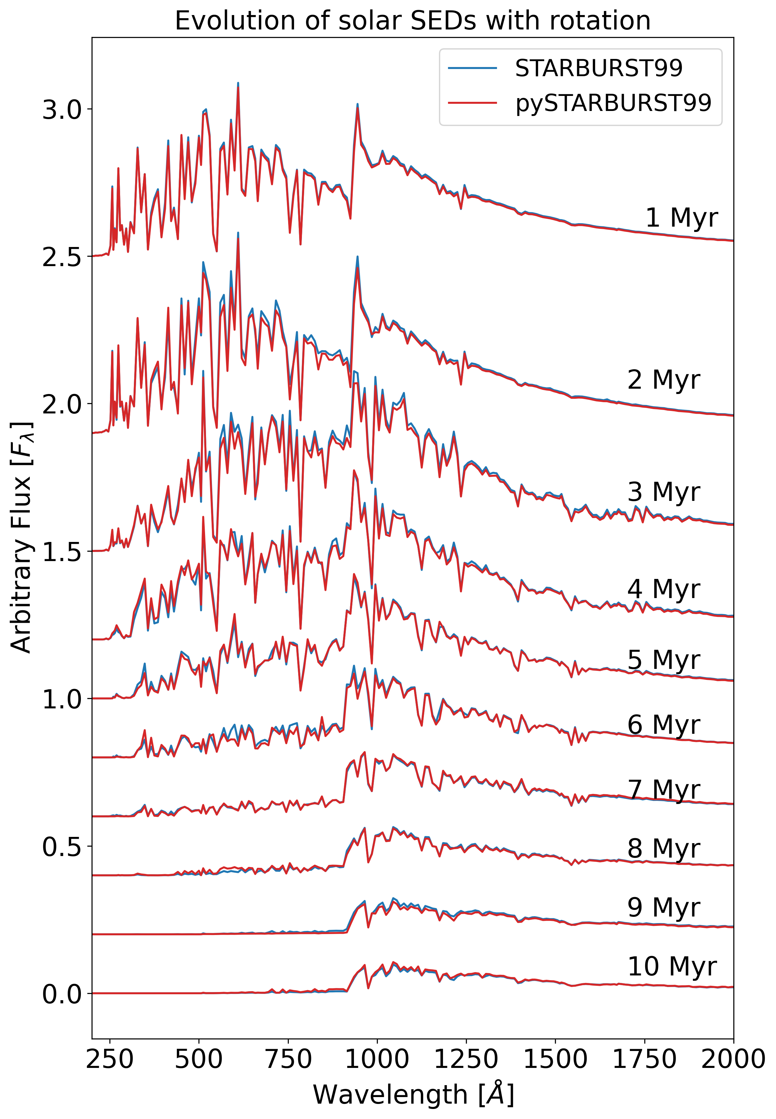
Figure 23: Synthetic FUV SEDs from Starburst99  compared to those produced with pyStarburst99, in both cases utilising the Ekström et al. (2012) stellar evolutionary models including rotation at Z=0.014 and WMbasic  spectra at Z=0.2. The evolution with time is shown from 1 Myr to 10 Myr at intervals of 1 Myr.

With the updates described in Sect. 2, there are a number of comparisons we can make with respect to computing SEDs. The first is to assess the quality of the SEDs produced with the python version of Starburst99  in comparison to the Fortran  version. For this task, we include only the well established stellar models used in previous versions of Starburst99, i.e., with the Genec  and WMbasic  models included in earlier studies (e.g., Levesque et al., 2012) and using a Kroupa IMF (Kroupa, 2002) with an upper mass limit of 120$M_{\odot{}}$. In Fig. 3 we show an example for such a population at various times and for non-rotating evolutionary models and include the comparison with rotation in Fig. 23. The agreement between both versions of the code is very good with any significant variations in flux being associated with differences in the output time of the stellar population, due to the precision of the time increment, which in turn affects the output at a given time. For example, an output spectrum from SB99 at 1.01Myr can have flux differences up to 300% at short wavelengths ($<1000$Å ) over a range of $50\,$Å compared to the 1.01Myr pyStarburst99 spectrum, whereas the pyStarburst99 output at 1.04Myr is within 5% of the SB99 1.01Myr spectrum with small spikes of 25% in the residuals on the scale of only 1 resolution element in wavelength. Such small scale discrepancies can be attributed to slight differences in the numerical solutions of the interpolation between stellar evolutionary tracks in the two versions of the code. The inclusion of additional masses in the evolutionary grids can also have an impact on the SEDs due to a resulting difference in the isochrones in either code version. The agreement between output SEDs from SB99 and pyStarburst99 has been tested and verified for solar, LMC, and SMC models as defined in the current version of Starburst99, with more comparisons shown in Appendix C.

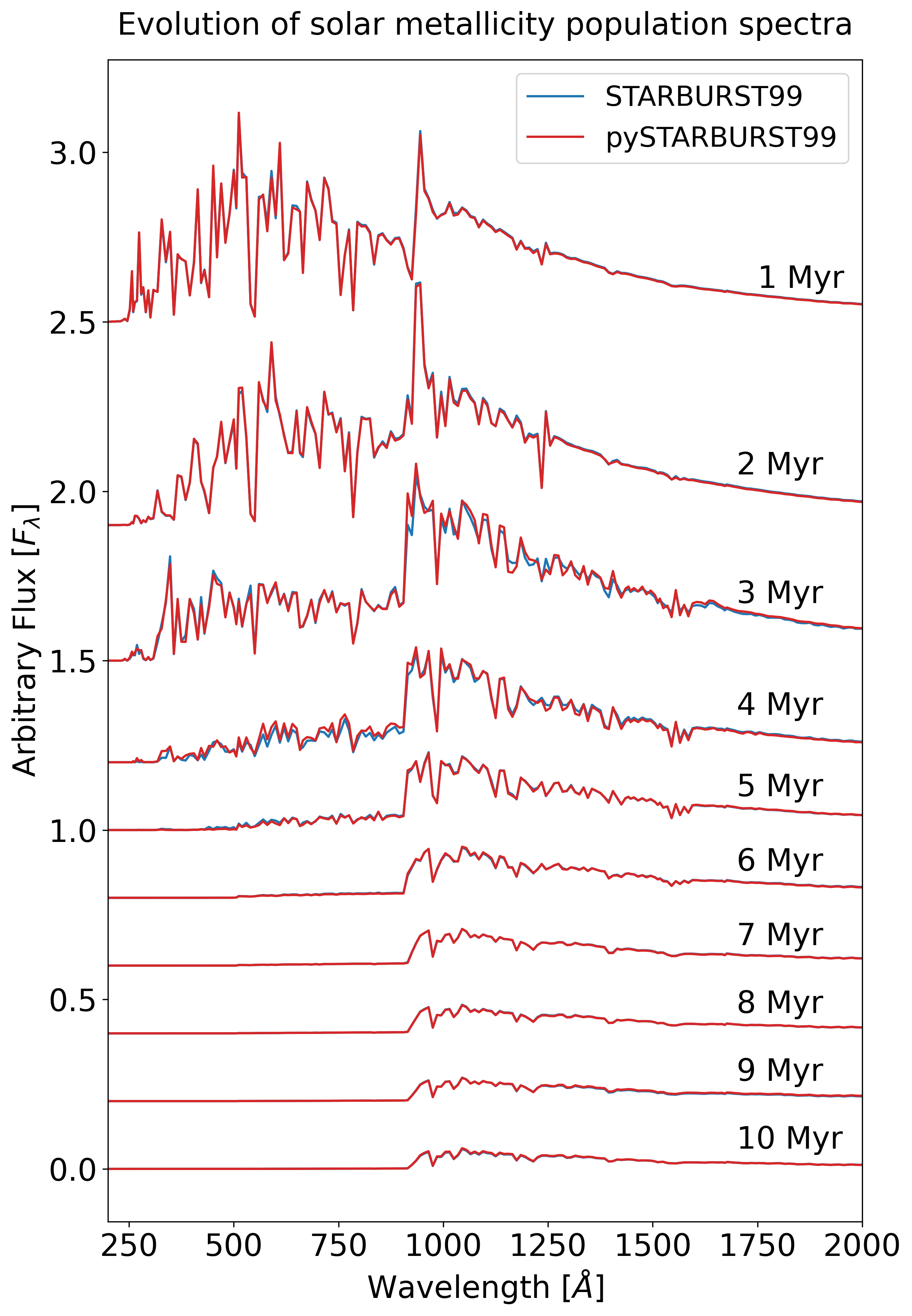
Figure 3: Synthetic FUV SEDs from Starburst99  compared to those produced with pyStarburst99  in both cases utilising the Ekström et al. (2012) stellar evolutionary models at Z=0.014 and WMbasic  spectra at Z=0.02. The evolution with time is shown from 1 Myr to 10 Myr at intervals of 1 Myr.

With the verification of pyStarburst99, our next step is to make a comparison between SEDs produced with Fastwind  models and those with WMbasic  models, keeping the evolutionary models consistent. It is difficult to provide a quantitative assessment of the difference between SEDs produced with pyStarburst99 using WMbasic  and Fastwind  spectra as there are significant differences in the fluxes on scales of $\sim$10Å  in the UV (as shown in Fig. 4), despite all input spectra being resampled to same wavelength grid. Qualitatively, it appears as though Fastwind  offers a much smoother SED below $\sim$1500Å  which may reduce the uncertainties in SED fitting to observed spectra. There are also specific limitations to certain aspects of the WMbasic spectra, for example the peak at 930Åis a known artifact due to the lack of pressure broadening in the models. For a few example SEDs in the model grid we also compare the Fastwind  and WMbasic  models with powr  models, resampled to the same wavelength grid, and find good agreement between powr  and Fastwind.

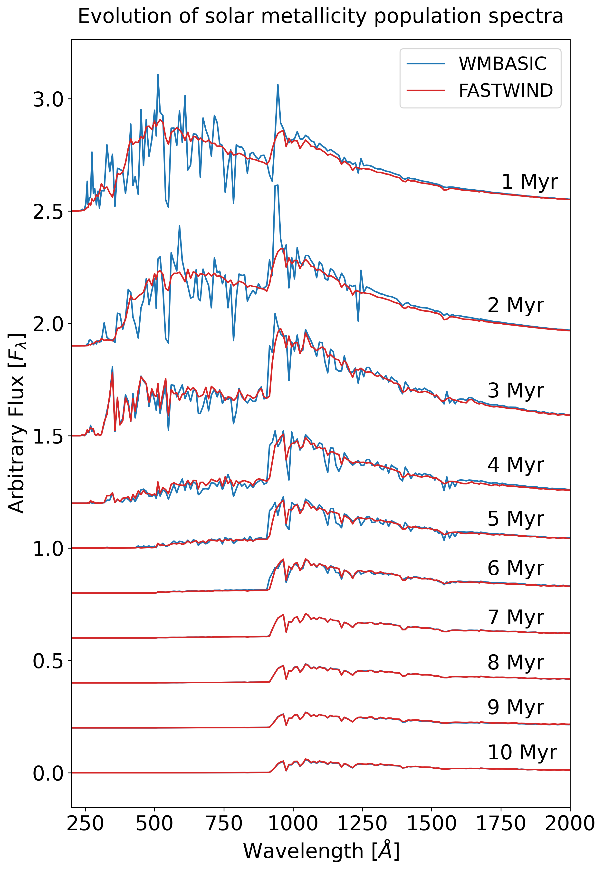
Figure 4: Synthetic FUV SEDs, utilising the Ekström et al. (2012) stellar evolutionary models at $Z=0.014$ for both, with WMbasic  spectra at $Z=0.02$ compared with Fastwind  spectra at $Z=0.014$. The evolution with time is shown from 1 Myr to 10 Myr at intervals of 1 Myr.

Using the Fastwind spectra as well as atmosphere models consistent with the metallicity of the employed Genec stellar evolution models, we can produce new population SEDs for all the newly available metallicities. In Fig. 5, we can see a clear trend in the peak of the SED flux shifting to shorter wavelengths at lower metallicity. The bolometric luminosity is held constant for this comparison, showing the effect of lower metallicity resulting in overall higher temperatures for the stellar population at a given time.

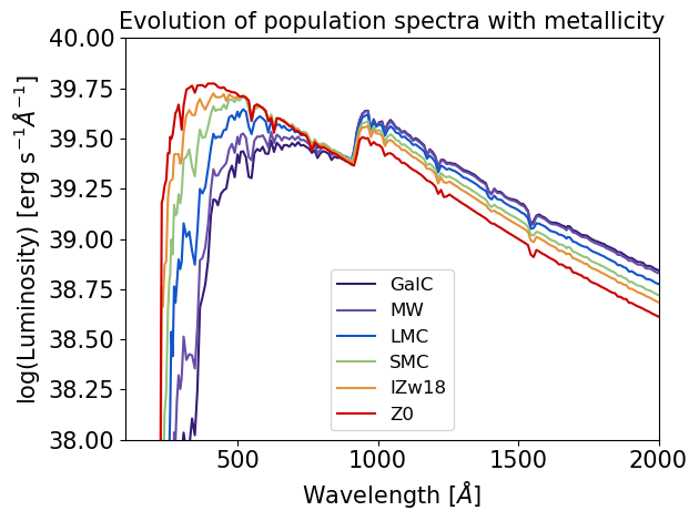
Figure 5: Low resolution synthetic SEDs with metallicities representative of populations in the Galactic centre to zero metallicity. These are produced at 2Myr using pyStarburst99 with the Genec  tracks, new Fastwind  model grid, an upper mass limit of 120$\rm M_{\odot}$ and no rotation.

Finally, we can investigate the impact of the inclusion of VMS in the SEDs. This is shown in Fig. 6, where we do not modify the slope of the upper IMF and simply extend the upper mass limit. There is a significant increase in flux which peaks in the FUV at early times and shifts to longer UV wavelengths before all the VMS have reached the end of core carbon burning by 3 Myr.

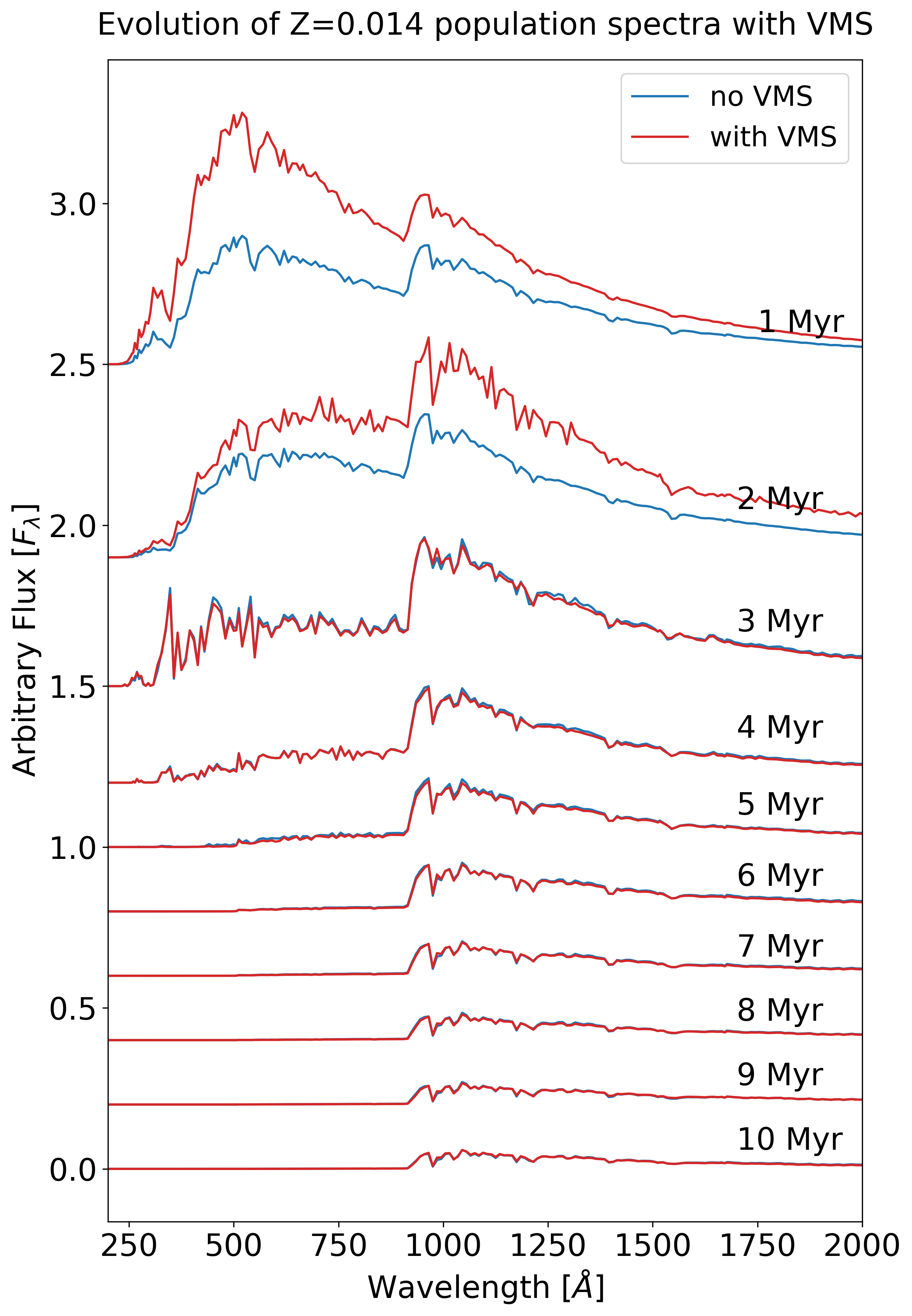
Figure 6: Synthetic FUV SEDs from pyStarburst99, utilising the Ekström et al. (2012) stellar evolutionary models at Z=0.014 and Fastwind  spectra at Z=0.014. This is compared with the addition of VMS evolutionary tracks up to $300M_{\odot}$ from Martinet et al. (2023) and Fastwind  models tailored to match the extended parameter space coverage from VMS evolutionary tracks. The evolution with time is shown from 1 Myr to 10 Myr at intervals of 1 Myr.

3.2 Ionising fluxes

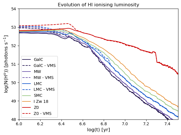
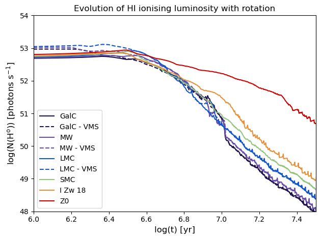
Figure 7: H I ionising fluxes with metallicity from solar to zero metallicity. The solid lines show H I ionising fluxes made with Fastwind  models and upper mass limit of 120$\rm M_{\odot}$, without rotation. The dashed lines are as the solid lines but with an upper mass limit of 300$\rm M_{\odot}$.

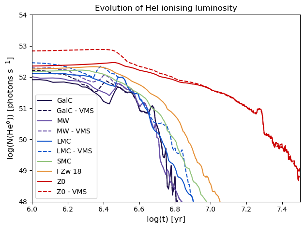
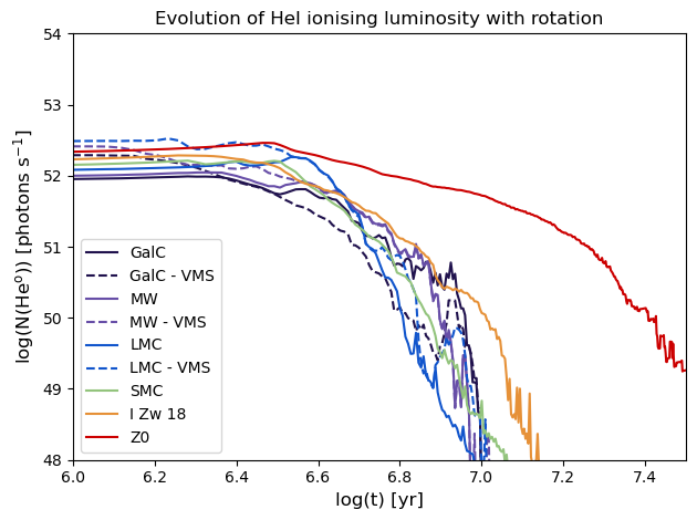
Figure 8: He I ionising fluxes as in Fig. 7.

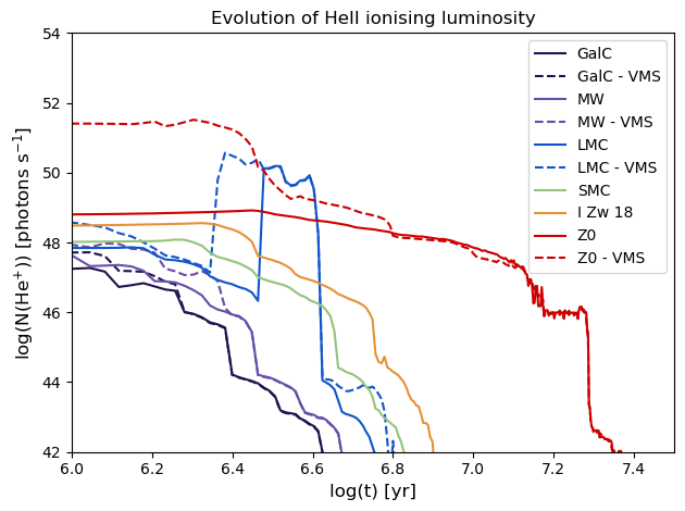
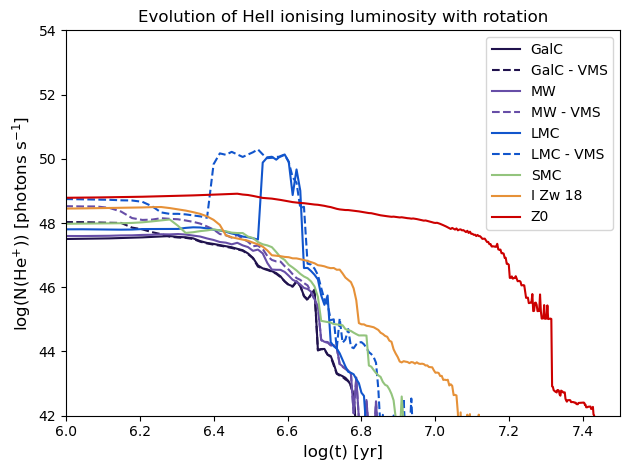
Figure 9: He II ionising fluxes as in Fig. 7.

Of particular interest in the study of starburst galaxies is the nature of the ionising spectrum, which can be greatly impacted by the intrinsic metallicity, as well as assumptions about the composition and evolution of the synthetic stellar population. Significant changes can be caused by the accounting and treatment of rotation (Levesque et al., 2012; Leitherer et al., 2014), binarity (Götberg et al., 2020), abundances (Grasha et al., 2021), and the presumed upper mass limit (Schaerer et al., 2024). The resulting uncertainty in the predicted ionising fluxes propagates into all simulations building on these results, such as photoionisation models and large-scale hydrodynamical simulations. The ionising photon production becomes even more important in the early Universe when Lyman continuum emitting galaxies contributed significantly to the reionisation of the Universe, particularly the reionisation of hydrogen. Yet, also the escape fraction must be taken into consideration. While this is beyond the scope of the present work, where we focus on the resulting intrinsic spectra of stellar populations with the updated version of Starburst99, escape fractions for massive star populations are an active field of theoretical and observational research and have for example recently been discussed in Izotov et al. (2016); Chisholm et al. (2018); Götberg et al. (2020); Pahl et al. (2020); Kimm et al. (2022); Marques-Chaves et al. (2022); Flury et al. (2022); Roy et al. (2024).

The behaviour of ionising fluxes with time (shown in Fig. 7) correlates well with the evolution of the stellar population. For the first $\sim$$2\,$Myr, the H I ionising flux is essentially constant as the stars at the upper end of the IMF expand while the maximum luminosity of the most massive stars increases. There is then a down-turn as the maximum temperature dips below 40 kK and the most massive stars expand more rapidly, until around 2.5 Myr when there is an uptick in H I ionising flux when the most massive stars enter post-MS evolution and are predicted to produce hot WR stars which have lost a considerable part of their hydrogen envelope. The H I ionising flux reaches a secondary peak around 3.1 Myr, which is immediately followed by the first supernova and a steady decrease in H I ionising flux as stars with decreasing initial masses reach the end of their evolution. This general trend is true for stellar populations at all metallicities, with the exception of the lack of the WR bump once the metallicity, and therefore wind strength, becomes too low for non-rotating single stars to enter the WR phase.

When comparing with the original Starburst99  outputs, care has to be taken to be consistent with respect to the metallicity of the evolution models and employed spectral atmosphere models. For example, one could observe a slight increase in ionising flux at solar metallicity in pyStarburst99 compared to Starburst99. This is due to the stellar library from WMbasic  being computed at $Z=0.02$ while the new Fastwind grid uses $Z=0.014$.

At all metallicities, the initial H I ionising flux is roughly constant, with a slightly higher ionising flux at early times for lower metallicities (differing by $0.015\,$dex between the most extreme metallicities). At later times, the ionising flux steadily decreases, but for any given time after $\sim$3 Myr, the ionising flux will be much higher at lower metallicity. This trend is a result of the difference in stellar evolution with metallicity. Notably, the input metallicity has essentially no impact on the hydrogen ionising flux of an individual stellar atmosphere model if all other stellar parameters are held constant. While there is less line-blanketing in the atmospheres of lower metallicity stars, photons which experience more scattering and absorption are eventually emitted at similar energies to their initial energy (Mokiem et al., 2004). This even holds for WR stars (Sander & Vink, 2020), but is no longer true for helium ionising photons. The physical process resulting in harder ionising hydrogen spectra at low metallicity comes from the fact that stars are in general hotter and more luminous when the metallicity decreases. Due to the dearth of the CNO cycle the stars must be denser and hotter to reach thermal equilibrium. There is an also a secondary opacity effect, in that lowered opacity increases the luminosity to mass ratio. Overall, the low metallicity star is hotter at similar luminosity (Mowlavi et al., 1998). Additionally, the zero metallicity population produces much higher ionising flux at late times compared to stars with any initial metal content. These stars do not become significantly more luminous, but metal-free stars must contract more than higher metallicity stars, until sufficient He is burnt in the core to trigger the CNO cycle. The onset of the CNO cycle is accompanied by a change of slope in the HRD: while contraction goes up-bluewards, when the CNO ignites, the star starts evolving up-redwards. Above 30 $\rm M_{\odot}$, this happens already before the ZAMS and the evolution is directly redwards from the ZAMS on. This extreme contraction results in much higher temperatures, for example, a $20M_{\odot}$ star reaches 65 kK at the ZAMS. This is 20 kK hotter than a $20M_{\odot}$ star with SMC metallicity. These stars also remain hotter for the full duration of their evolution: A $30M_{\odot}$ star never drops below 25 kK at zero metallicity, meaning that the ionising flux output remains comparably high throughout the full lifetime.

The initial ionising flux output only increases with the upper mass limit. If we increase the upper mass limit to the maximum covered by the Genec  tracks ($500\,M_{\odot}$ at Z=0.014 and $300\,M_{\odot}$ at Z=0.006 and 0.0), there is a corresponding increase in H I ionising flux by $\sim 0.4$ dex for $500\,M_{\odot}$ and $\sim 0.3$ dex for $300\,M_{\odot}$. The H I ionising flux quickly returns to that of a traditional population (upper mass limit of $120\,M_{\odot}$) once the VMS have disappeared within the first 3 Myrs.

With the addition of rotation to any specific population we see that the ionising fluxes stay higher for longer, due to a combination of two effects, first the increase in stellar lifetimes which comes with the rejuvenation of hydrogen in the core, and secondly the increase in temperature and luminosity which results from the larger convective core and lower surface opacity.

We observe very similar trends for the He I and He II ionising fluxes as we do for H I, with the boosts in ionising flux with rotation and VMS being more pronounced for He than H. We note the presence of a significant enhancement in He II ionising flux at LMC metallicity during the WR lifetime. This WR bump is not present at lower metallicity due to the lack of WR stars predicted by single-star evolutionary tracks at low metallicity. However the WR bump is also not observed at higher metallicity were WR stars are predicted. There are two contributing factors to this, the main reason being that the WR synthetic spectral grids with $Z\geq 0.014$ show significantly less flux below 300Å  than lower metallicity models for the same spectral types. The secondary factor is that the LMC isochrones predict much more luminous (by $\sim 0.3$dex) WR stars than higher metallicity tracks. Therefore if the LMC WR spectra were not scaled to the luminosity of the isochrones and simply assigned, maintaining the input luminosity of closest stellar atmosphere model the WR bump would disappear.

We can also make predictions of the equivalent widths (EW) of key diagnostics at longer wavelengths (e.g. H$\alpha$, H$\beta$, Pa$\beta$, Br$\gamma$). The EW is defined as the ratio of the luminosity of these lines, which are estimated from the H I ionising flux, to the continuum flux at the wavelength of the transition. In Fig. 11 the general trend of H$\alpha$ EW is similar to the H I ionising flux in time and metallicity, but the behaviour differs with the addition of VMS. There is a similar increase in H$\alpha$ EW with the addition of VMS initially, but from 1.6 Myr to 2.2 Myr the H$\alpha$ EW actually decreases when VMS are included. This is caused by a large jump in the temperatures of the isochrones, with the VMS decreasing in temperature by 20 kK in a single timestep. This results in the sudden switch to a population of luminous ($\log(L_{*}/L_{\odot})$$>6.5$) but relatively cool ($\sim 20$ kK) stars, which provide high continuum fluxes with hardly any ionising flux. The trend in H$\alpha$ EW returns to normal after 2.2 Myr when WR stars are predicted.

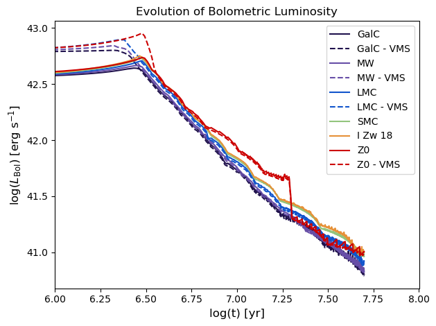
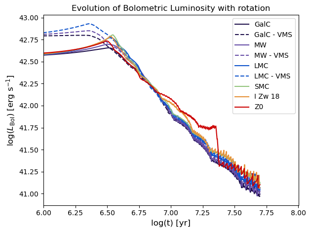
Figure 10: As described in Fig. 7 but showing bolometric luminosity.

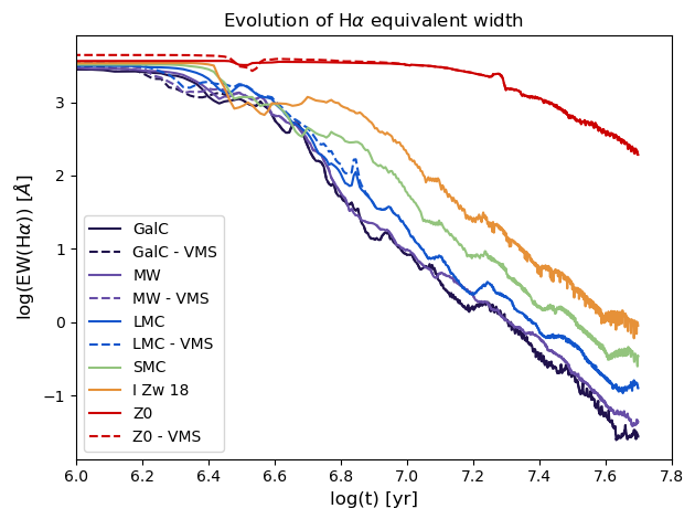
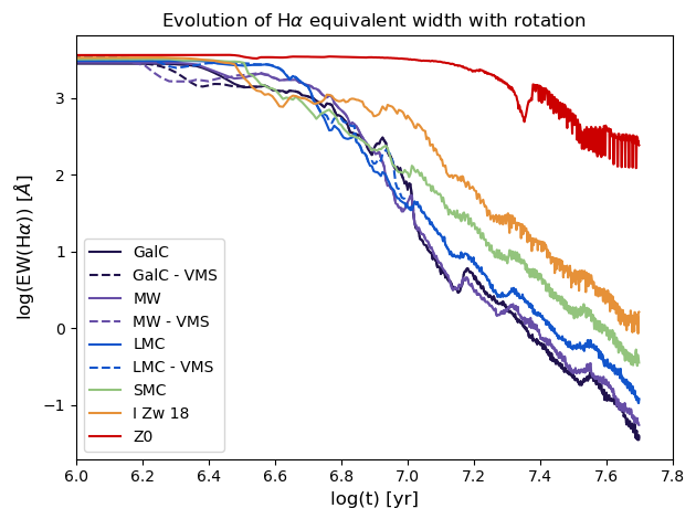
Figure 11: H$\alpha$ equivalent widths as in Fig. 7.

3.3 Wind power

Along with ionising processes, the mechanical output of massive stars is an important feedback mechanism, ejecting stellar masses worth of material at speeds on the order of thousands of $\rm{km\,s^{-1}}$. Such high energy outflows affect a number of Galaxy-scale processes, ranging from galaxy and star formation to driving galactic outflows. In addition, significant quantities of metals are deposited into the ISM.

The wind power computed with Starburst99 is a combination of the mass-loss rate and terminal wind speed summed over the full population. In Fig. 12, we show the evolution of the wind momentum ($\dot{M}$$v_{\infty}$) with age and metallicity. These predictions are computed using the inputs of the Genec  models themselves, which are the theoretical predictions of $\dot{M}$ from Vink et al. (2001) and $v_{\infty}$ from Leitherer et al. (1992) on the main sequence. In contrast to the predictions for the ionising flux, we see a decrease in wind power with decreasing metallicity. Such a trend is well established (Mokiem et al., 2007; Garcia et al., 2014; Bouret et al., 2015; Marcolino et al., 2022; Brands et al., 2022; Hawcroft et al., 2024a, b; Backs et al., 2024; Telford et al., 2024) and expected due to the reduction in line-driving that comes with the reduced number of metal ions in a stellar atmosphere (e.g. Vink et al., 2001; Krtička & Kubát, 2017; Björklund et al., 2021; Vink & Sander, 2021). At any given metallicity, the inclusion of VMS increases the wind power. With an upper mass limit of $300\,M_{\odot}$, we find an increase in wind momentum of $0.43$ and $0.47\,$dex for the predictions at $Z=0.014$ and $0.006$ respectively. The general trend in wind momentum with time is consistent across all metallicities and corresponds directly to changes in the mass-loss rate prescription used in the Genec  models. A notable deviation from the general trend are the predictions at zero metallicity. In this case, no mass is lost from the surface of the star in the Genec models unless the star reaches either the Eddington limit or critical rotation, at which point the mass-loss rate is increased significantly and is reflected in the non-rotating VMS models or typical masses with rotation. There are currently no estimates of $v_{\infty}$ for zero metallicity models and so to obtain an estimate for the wind power, we implement a metallicity of $Z=10^{-5}$, resulting in maximum $v_{\infty}$ values around 400 $\rm{km}\,\rm{s}^{-1}$  for the most extreme cases.

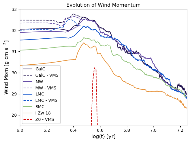
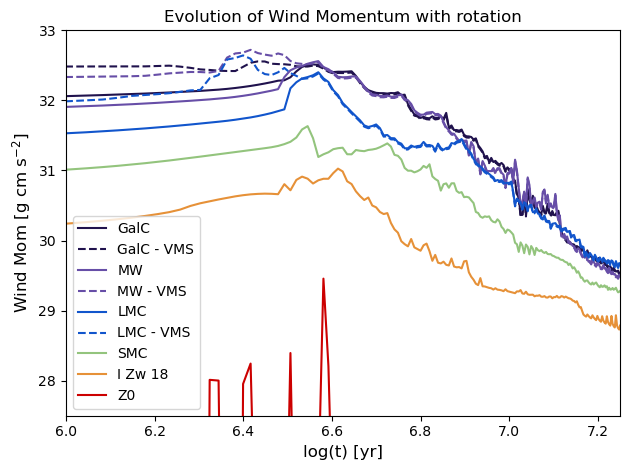
Figure 12: As described in Fig. 7 but showing wind momentum.

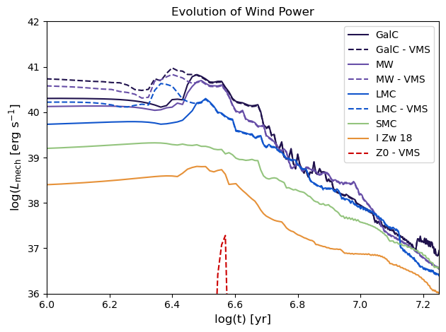
Figure 13: As described in Fig. 7 but showing wind power.

We can also make predictions for the wind power with new theoretical predictions and empirical calibrations for the wind strengths of massive stars as these can be applied directly to pre-computed isochrones. Although the alternate predictions have not been included in the evolutionary models and thus will not be be entirely consistent with the predicted HRD positions, applying them to the isochrones computed using the Vink et al. (2001) predictions gives us a first order of magnitude estimate of the impact of these updated prescriptions with respect to mechanical feedback. In the future, we aim to recompute these and other outputs with new evolutionary tracks tailored to our improved understanding of the wind properties of massive stars, ideally covering both the main sequence and post-MS stages.

For solar metallicity, the theoretical rates from Vink & Sander (2021) are very consistent with those from Vink et al. (2001) and thus have no impact on the wind momentum. When switching to theoretical mass-loss rates from Björklund et al. (2021), however, there is a significant decrease in wind momentum on the order of $0.8\,$dex at any given time within the first 2.5 Myr.

In the trend of wind momentum with metallicity, we can see that empirical terminal wind speed calibrations from Hawcroft et al. (2024a), which corresponds to a change from $Z^{0.13}$ to $Z^{0.22}$, has a relatively small impact, causing a downward shift in the wind momentum by $0.05$, $0.1$, and $0.15\,$dex in the LMC, SMC and IZw18 models respectively. This corresponds to a $0.08$, $0.12$, $0.18$ reduction in wind power.

3.4 UV slopes

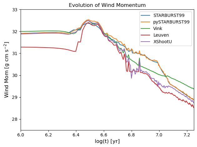
Figure 14: Wind momentum fluxes over time for a typical single stellar population with upper mass limit of 120$M_{\odot}$, no rotation comparing Starburst99 with pyStarburst99 and a few other mass loss and terminal wind speed recipes on the main sequence.

The UV slope power index $\beta$ (where $F_{\lambda}\propto\lambda^{\beta}$) is commonly used as a gauge of the reddening of the stars due to dust attenuation, making it a powerful diagnostic tool especially at high redshift.

We measure the $\beta$-slope with a linear fit in log space to the UV continuum in six windows across the range 1250Å  to 1750Å  as defined in Calzetti et al. (1994). We find the $\beta$-slope trend with age is fairly consistent between all metallicities with significant deviations from this general trend arising when VMS are included as a result of their more extreme UV continua. This effect is more prominent in predictions with rotation. For all metallicities, $\beta$ lies within a range of -2.5 to -2.3 in the first $\sim$2.5-3 Myr, with higher metallicities having steeper slopes and the $\beta$ value being essentially constant for any given metallicity. We then find a non-monotonic increase in steepness of the slope until $\sim$10 Myr, after which the slope steadily decreases.

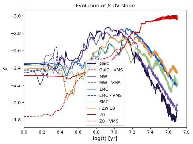
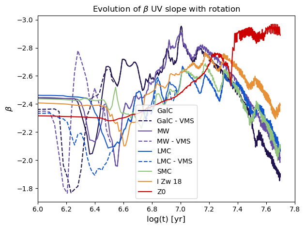
Figure 15: UV slopes computed from synthetic FUV SEDs, within the range 1250-1750Å, including the contribution from the nebular continuum.

4 Conclusions and future work

We have updated the Starburst99  population synthesis code through three major avenues to improve its capacity to reproduce or predict the properties of star-forming galaxies and maximise ease of use for the community. We first translated the software from Fortran  to python, and keeping in tradition with Starburst99, make the code publicly available on the Starburst99  website/github. Currently not all modules of Starburst99  are available in python but work to add these capabilities are ongoing. The published version will be subject to regular updates. The other two major updates are to expand the metallicity range available and to increase the upper mass limit for both rotating and non-rotating populations. We are now able to offer an updated metallicity grid ($Z=0.02,0.014,0.006,0.002,0.0004$ and $0.0$) and an extended upper mass limit to $300M_{\odot}$ for Z = 0.006 and 0.0 as well as models up to $500M_{\odot}$ at $Z=0.014$ and $0.02$. These updates have been made possible using the latest suite of Genec  stellar evolutionary models covering all the aforementioned metallicities and mass ranges both with and without the effects of rotation. We also generated a new library of synthetic spectra with the Fastwind  code to complement this extended grid coverage in stellar evolutionary predictions.

All the modules presented in this work are available for use in pyStarburst99  and the new stellar models have been implemented in the original Starburst99  Fortran  code. We aim to add other Starburst99  functions to pyStarburst99 and make them available as they are tested and verified. The main module still to come is predicting high resolution synthetic spectra for the full unresolved stellar population which requires a larger library of more computationally expensive stellar atmosphere models which are currently in progress. Additional further work includes updates to the empirical spectral library which can be significantly expanded at low metallicities thanks to the ULLYSES programme. We also plan to add the functionality to compute mixed age populations.

Within the scope of this work, we have been able to make predictions for a number of properties for integrated stellar populations and how they are impacted by the added new metallicities and the change of upper mass limits, along with rotation. These are: Low resolution spectra or SEDs from 90-10,000 Å, ionising fluxes of hydrogen and helium as well as bolometric luminosity and hydrogen line equivalent widths, wind power and momentum (which is further updated with input from the latest literature of hot star winds) and UV $\beta$-slopes.

We find that we are able to reproduce the results of the original Starburst99  models, including Genec  models produced up to 2014 and the WMbasic  model atmosphere grid from Leitherer et al. (2010), and are therefore confident in making predictions with new stellar atmosphere (Fastwind  v10) and evolutionary (Genec  up to 2023) models with pyStarburst99.

We find a steady shift in the peak SED flux to shorter wavelengths with decreasing metallicity at constant luminosity. As an example, for a 2 Myr old instantaneous burst, flux levels below 900 Å increase by roughly a factor of two from solar to zero metallicity and the fluxes above 900 Å decrease to compensate, although the shift above 900 Å  is much lower and becomes less significant with increasing wavelength. Therefore the ionising flux of hydrogen (and helium) also increases with decreasing metallicity. Metal free populations have significantly higher ionising flux than other predictions at late times. Predictions with rotation maintain high ionising fluxes for slightly longer than non-rotating models due to the increase in stellar lifetime. The addition of VMS increases the ionising flux of any population, but only at early times (less than 3 Myr). The wind momentum decreases with decreasing metallicity but is boosted at early times if VMS are included. There is a more complex trend of the $\beta$-slope with age but generally higher metallicity populations have steeper UV slopes and the steepest slopes are observed in the first $\sim$10 Myr.

We would also like to highlight the limitations of population synthesis with only single star models. It is well established that almost all of the most massive stars are in binary systems Sana et al. (2013), with over 50% of these stars expected to undergo an interaction throughout their evolution Sana et al. (2012); Kummer et al. (2023). The impact of binarity is more pertinent for many of the global properties of stellar populations that aren’t extensively discussed in this work, e.g. rates of supernova and compact object coalescence, but binary interaction is also important for the properties presented here particularly at later times (population ages $>10$Myr). For example, Eldridge et al. (2017) predict at least an order of magnitude increase in ionising flux output at 50Myr with the inclusion of binary systems in the BPASS code, with Götberg et al. (2019) finding similar increases when adding a population of stripped stars to Starburst99 models. Since we find the inclusion of rotation provides the strongest boost to ionising flux, similarly to Byler et al. (2017), at earlier times (from roughly 3Myr to 10Myr, with an almost 1 dex increase for a 6Myr population) it is clear that parameter studies with single star populations can still offer valuable insights. However, efforts to combine multiple important effects for massive star populations, including metallicity, the upper mass limit, rotation and binarity are incredibly important and will be essential to gain a complete picture of stellar populations throughout the universe. Binary interaction should not have a significant impact on the wind luminosity of a stellar population (excluding SN feedback), although non-conservative mass transfer could result in a small boost to wind yields during the stellar lifetime. Götberg et al. (2019) predict that the H$\alpha$ EW is not strongly impacted by binary interaction in constant star formation scenarios, but that binary stripping has a significant impact on nebular H$\alpha$ if star forming has stopped for more than 10Myr. A similar impact is shown for a wider range of nebular diagnostics in e.g. Xiao et al. (2018); Lecroq et al. (2024). Götberg et al. (2019) also note that $\beta$ is not impacted by binary interaction below 100Myr, meaning single star predictions provide sufficient and robust for measurements of the UV slope for young populations.

Within this paper we do not provide much comparison to observations, in the interest of releasing the models and code as soon as possible. A few ready applications of these updated models for low metallicity and/or including VMS are to help to better reproduce the global properties of extreme populations at high redshift, for example increased ionising flux Llerena et al. (2024); Muñoz et al. (2024) and extreme UV slopes Kumari et al. (2024); Dottorini et al. (2024); Cullen et al. (2025); Fujimoto et al. (2025). However, an extensive assessment of the ability of the updated models to reproduce the observed properties of stellar populations is beyond the scope of this work, but is planned for an upcoming publication. We also plan to discuss the rest-frame UV spectra of star-forming galaxies in a future work which will update the theoretical and empirical high-resolution stellar libraries used in pyStarburst99. Further work is also planned to interpret nebular diagnostics using photoionisation models produced from pyStarburst99 SEDs (Aranguré et al. in prep.)

There are a number of additional Starburst99 modules which have not been presented in this work, some of which have already been implemented in the pyStarburst99 code and can reproduce Starburst99 outputs but further updates are planned for these modules, while others have not yet been implemented. The high resolution UV spectral synthesis, spectral type, supernova rate and colour predictions are all in the former state. The optical spectral synthesis, empirical spectral synthesis, line equivalent width and chemical yield routines are in the latter case. In these appendices we present an example prediction of colours using pyStarburst99. The UV spectral synthesis will be presented in an upcoming work with the incorporation of a new grid of high resolution theoretical spectra. The spectral type module is available in the pyStarburst99 code but will be updated with new spectral type calibrations. The implementation of the remaining modules is still in progress but regular updates will be provided on the pyStarburst99 webpage.

Appendix A Example values

Here we present tables of example output values for the predictions shown in Figs 7 - 15.

Table 2: H I ionising fluxes in units of photons s^-1.

t	GalC	MW	LMC	SMC	IZw18	Z0	GalC	MW	LMC	SMC	IZw18	Z0	GalC	MW	LMC	Z0	GalC	MW	LMC
[Myr]	v00	v00	v00	v00	v00	v00	v40	v40	v40	v40	v40	v40	M300	M300	M300	M300	M300v40	M300v40	M300v40
1.0	52.68	52.71	52.74	52.77	52.78	52.82	52.69	52.70	52.73	52.75	52.76	52.80	52.96	52.99	53.04	53.08	52.97	53.02	53.05
1.6	52.67	52.69	52.76	52.80	52.82	52.85	52.71	52.73	52.76	52.79	52.80	52.84	52.90	52.99	53.02	53.10	52.97	53.02	53.07
2.5	52.43	52.52	52.67	52.80	52.87	52.91	52.73	52.77	52.84	52.85	52.84	52.90	52.63	52.74	52.88	53.17	52.76	52.90	53.10
4.0	52.05	52.15	52.30	52.36	52.46	52.72	52.56	52.69	52.82	52.63	52.58	52.78	52.03	52.14	52.32	52.73	52.52	52.67	52.81
6.3	50.97	51.07	51.37	51.64	51.84	52.38	51.94	52.01	51.89	51.94	52.05	52.47	50.95	51.06	51.45	52.37	51.88	52.00	52.05
10.0	49.81	49.98	50.26	50.55	50.90	52.11	50.90	50.66	50.67	51.00	51.53	52.23	49.79	49.96	50.24	52.08	50.89	50.64	50.74
15.8	48.86	49.06	49.29	49.53	49.80	51.70	49.39	49.41	49.65	49.97	50.23	51.81	48.85	49.04	49.27	51.69	49.30	49.40	49.66
25.1	48.07	48.25	48.57	48.80	49.05	50.92	48.49	48.59	48.84	49.14	49.38	51.11	48.05	48.23	48.55	50.90	48.43	48.58	48.84

Table 3: He I ionising fluxes in units of photons s^-1.

t	GalC	MW	LMC	SMC	IZw18	Z0	GalC	MW	LMC	SMC	IZw18	Z0	GalC	MW	LMC	Z0	GalC	MW	LMC
[Myr]	v00	v00	v00	v00	v00	v00	v40	v40	v40	v40	v40	v40	M300	M300	M300	M300	M300v40	M300v40	M300v40
1.0	51.91	52.01	52.11	52.18	52.25	52.35	51.95	52.00	52.08	52.15	52.23	52.34	52.22	52.29	52.46	52.84	52.29	52.41	52.49
1.6	51.81	51.89	52.08	52.21	52.29	52.38	51.97	52.03	52.11	52.19	52.27	52.37	52.02	52.21	52.31	52.86	52.22	52.29	52.50
2.5	51.22	51.51	51.83	52.09	52.31	52.44	51.93	52.00	52.20	52.20	52.24	52.43	51.80	52.05	52.31	52.89	51.91	52.10	52.47
4.0	51.14	51.17	51.48	51.48	51.78	52.24	51.73	51.87	52.16	51.81	51.85	52.29	51.12	51.15	51.48	52.36	51.46	51.86	52.16
6.3	48.47	48.49	49.17	50.03	50.80	51.91	50.76	50.98	50.37	50.64	51.15	51.99	48.45	48.48	49.65	51.98	50.11	50.96	50.88
10.0	46.01	46.44	47.16	47.83	48.63	51.63	48.67	47.30	47.90	48.63	50.21	51.74	45.99	46.42	47.14	51.64	48.73	47.29	48.61
15.8	44.11	44.62	45.39	46.02	46.69	51.07	45.15	45.19	45.94	46.78	47.39	51.24	44.09	44.60	45.37	51.07	44.92	45.18	45.98
25.1	41.70	42.49	43.69	44.47	45.26	49.83	42.77	43.35	44.20	45.14	45.86	50.12	41.68	42.47	43.67	49.74	42.69	43.33	44.20

Table 4: He II ionising fluxes in units of photons s^-1.

t	GalC	MW	LMC	SMC	IZw18	Z0	GalC	MW	LMC	SMC	IZw18	Z0	GalC	MW	LMC	Z0	GalC	MW	LMC
[Myr]	v00	v00	v00	v00	v00	v00	v40	v40	v40	v40	v40	v40	M300	M300	M300	M300	M300v40	M300v40	M300v40
1.0	47.25	47.60	47.84	48.02	48.48	48.80	47.50	47.60	47.80	47.98	48.45	48.79	47.71	47.92	48.57	51.41	48.03	48.52	48.75
1.6	46.74	46.89	47.65	48.04	48.52	48.83	47.55	47.63	47.81	48.02	48.49	48.82	47.03	47.71	47.82	51.46	47.80	48.10	48.66
2.5	44.22	45.93	46.80	47.47	48.37	48.89	47.35	47.47	47.79	47.80	48.10	48.88	44.20	45.92	50.48	51.23	47.33	47.80	49.83
4.0	42.80	43.09	49.93	46.35	46.93	48.65	46.18	46.48	50.13	46.85	46.95	48.70	42.79	43.08	49.91	49.23	46.19	46.66	50.12
6.3	37.74	38.57	40.54	42.84	44.37	48.29	41.55	41.92	43.01	44.50	44.88	48.36	37.72	38.56	41.13	48.47	41.41	41.90	44.28
10.0	-	-	-	37.82	39.46	47.89	35.63	34.24	37.59	39.80	43.51	48.02	-	-	-	47.78	35.72	34.22	40.03
15.8	-	-	-	-	-	45.98	-	-	-	36.08	37.67	46.92	-	-	-	45.95	-	-	-
25.1	-	-	-	-	-	41.91	-	-	-	-	-	42.40	-	-	-	41.79	-	-	-

Table 5: Bolometric luminosities in units of log$L_{\rm{Bol}}$ erg s_-1.

t	GalC	MW	LMC	SMC	IZw18	Z0	GalC	MW	LMC	SMC	IZw18	Z0	GalC	MW	LMC	Z0	GalC	MW	LMC
[Myr]	v00	v00	v00	v00	v00	v00	v40	v40	v40	v40	v40	v40	M300	M300	M300	M300	M300v40	M300v40	M300v40
1.0	42.58	42.58	42.59	42.60	42.60	42.61	42.57	42.58	42.58	42.59	42.59	42.60	42.79	42.81	42.82	42.82	42.79	42.81	42.83
1.6	42.59	42.61	42.62	42.63	42.64	42.64	42.60	42.61	42.62	42.62	42.63	42.63	42.80	42.82	42.86	42.85	42.80	42.83	42.88
2.5	42.63	42.65	42.67	42.69	42.70	42.70	42.63	42.66	42.69	42.69	42.69	42.69	42.76	42.80	42.86	42.91	42.78	42.83	42.91
4.0	42.41	42.44	42.49	42.51	42.50	42.53	42.58	42.65	42.69	42.69	42.66	42.59	42.39	42.42	42.47	42.51	42.56	42.63	42.68
6.3	42.08	42.10	42.14	42.17	42.17	42.19	42.30	42.33	42.32	42.32	42.31	42.28	42.06	42.08	42.13	42.18	42.28	42.31	42.31
10.0	41.74	41.77	41.82	41.84	41.85	41.96	41.93	41.94	41.97	41.98	42.04	42.08	41.73	41.75	41.80	41.94	41.91	41.92	41.95
15.8	41.43	41.45	41.52	41.57	41.57	41.69	41.64	41.65	41.68	41.67	41.70	41.82	41.41	41.44	41.50	41.68	41.60	41.63	41.64
25.1	41.23	41.20	41.29	41.36	41.36	41.23	41.36	41.39	41.45	41.44	41.48	41.33	41.22	41.18	41.28	41.23	41.34	41.37	41.40

Table 6: H$\alpha$ equivalent widths in units of Å.

t	GalC	MW	LMC	SMC	IZw18	Z0	GalC	MW	LMC	SMC	IZw18	Z0	GalC	MW	LMC	Z0	GalC	MW	LMC
[Myr]	v00	v00	v00	v00	v00	v00	v40	v40	v40	v40	v40	v40	M300	M300	M300	M300	M300v40	M300v40	M300v40
1.0	3.45	3.47	3.50	3.51	3.53	3.56	3.45	3.46	3.49	3.51	3.53	3.56	3.49	3.51	3.54	3.65	3.51	3.53	3.55
1.6	3.41	3.43	3.48	3.52	3.53	3.56	3.45	3.46	3.49	3.51	3.53	3.56	3.38	3.46	3.49	3.65	3.45	3.43	3.51
2.5	3.08	3.17	3.32	3.45	3.52	3.56	3.37	3.38	3.48	3.50	3.49	3.56	3.09	3.19	3.28	3.64	3.17	3.22	3.46
4.0	2.83	2.83	3.04	2.97	2.99	3.54	3.11	3.27	3.42	3.13	3.03	3.53	2.83	2.84	3.07	3.58	3.11	3.27	3.43
6.3	1.72	1.81	2.08	2.54	2.99	3.54	2.78	2.87	2.59	2.67	2.96	3.54	1.72	1.81	2.17	3.57	2.78	2.87	2.75
10.0	0.94	0.99	1.33	1.85	2.35	3.52	1.89	1.56	1.63	2.06	2.77	3.51	0.94	0.99	1.33	3.52	1.89	1.56	1.69
15.8	0.18	0.41	0.39	0.90	1.44	3.41	0.74	0.56	0.92	1.43	1.83	3.37	0.18	0.41	0.39	3.41	0.74	0.56	0.92
25.1	-0.46	-0.19	-0.05	0.22	0.76	3.06	-0.21	-0.02	0.17	0.71	1.14	3.17	-0.46	-0.19	-0.05	3.06	-0.21	-0.02	0.17

Table 7: Wind powers in units of log$L_{\rm{mech}}$ erg s_-1.

t	GalC	MW	LMC	SMC	IZw18	Z0	GalC	MW	LMC	SMC	IZw18	Z0	GalC	MW	LMC	Z0	GalC	MW	LMC
[Myr]	v00	v00	v00	v00	v00	v00	v40	v40	v40	v40	v40	v40	M300	M300	M300	M300	M300v40	M300v40	M300v40
1.0	40.30	40.13	39.73	39.20	38.40	-	40.32	40.14	39.69	39.08	38.16	-	40.73	40.58	40.22	33.73	40.75	40.57	40.16
1.6	40.29	40.13	39.78	39.28	38.49	-	40.33	40.17	39.75	39.16	38.28	-	40.65	40.50	40.16	33.76	40.70	40.53	40.19
2.5	40.28	40.11	39.76	39.29	38.59	-	40.37	40.22	39.81	39.25	38.47	35.07	40.98	40.83	40.57	33.99	40.65	40.86	40.73
4.0	40.30	40.16	39.84	39.06	38.42	-	40.64	40.63	40.36	38.98	38.30	35.27	40.29	40.15	39.83	34.16	40.62	40.61	40.35
6.3	38.77	38.84	38.95	38.30	37.33	-	39.89	39.95	39.00	38.57	37.46	-	38.75	38.82	38.93	33.72	39.87	39.94	38.98
10.0	37.98	38.30	37.91	37.63	36.88	-	39.05	38.70	38.49	37.77	36.91	-	37.97	38.29	37.89	33.49	39.04	38.68	38.47
15.8	37.27	36.85	36.61	36.90	36.36	-	37.59	37.45	37.48	37.08	36.48	-	37.25	36.83	36.59	33.47	37.57	37.43	37.46
25.1	36.48	36.19	35.79	36.12	35.63	-	36.65	36.50	36.64	36.38	35.75	-	36.47	36.17	35.77	32.57	36.63	36.48	36.62

Table 8: $\beta$ UV slopes.

t	GalC	MW	LMC	SMC	IZw18	Z0	GalC	MW	LMC	SMC	IZw18	Z0	GalC	MW	LMC	Z0	GalC	MW	LMC
[Myr]	v00	v00	v00	v00	v00	v00	v40	v40	v40	v40	v40	v40	M300	M300	M300	M300	M300v40	M300v40	M300v40
1.0	-2.44	-2.45	-2.45	-2.42	-2.40	-2.31	-2.44	-2.45	-2.45	-2.42	-2.40	-2.31	-2.37	-2.37	-2.34	-1.84	-2.36	-2.35	-2.33
1.6	-2.44	-2.46	-2.45	-2.42	-2.39	-2.31	-2.44	-2.46	-2.45	-2.42	-2.39	-2.31	-2.26	-2.32	-2.39	-1.84	-1.88	-1.76	-2.27
2.5	-2.53	-2.47	-2.44	-2.41	-2.37	-2.30	-2.53	-2.47	-2.44	-2.41	-2.37	-2.30	-2.45	-2.39	-2.33	-1.92	-2.46	-2.51	-1.89
4.0	-2.51	-2.46	-2.45	-2.35	-2.32	-2.31	-2.51	-2.46	-2.45	-2.35	-2.32	-2.31	-2.51	-2.45	-2.44	-2.25	-2.72	-2.31	-2.18
6.3	-2.78	-2.67	-2.51	-2.53	-2.58	-2.40	-2.78	-2.67	-2.51	-2.53	-2.58	-2.40	-2.78	-2.67	-2.46	-2.46	-2.58	-2.54	-2.33
10.0	-2.84	-2.77	-2.64	-2.64	-2.74	-2.51	-2.84	-2.77	-2.64	-2.64	-2.74	-2.51	-2.84	-2.77	-2.64	-2.58	-2.88	-2.89	-2.52
15.8	-2.60	-2.74	-2.82	-2.46	-2.67	-2.80	-2.60	-2.74	-2.82	-2.46	-2.67	-2.80	-2.60	-2.74	-2.82	-2.80	-2.73	-2.76	-2.58
25.1	-2.28	-2.41	-2.62	-2.44	-2.56	-2.93	-2.28	-2.41	-2.62	-2.44	-2.56	-2.93	-2.28	-2.41	-2.62	-2.93	-2.50	-2.57	-2.54

Appendix B Colours

pyStarburst99 can produce predictions for all colours as defined in Starburst99, these include the F130M, F210M, U, B, V, R, I, J, H, K and L bands. We also intend to extend the colours available in pyStarburst99. Here, as an example, we show a comparison of $M_{V}$ predicted from pyStarburst99 including all stars between $120M_{\odot}$ and $300M_{\odot}$. A significant increase in $M_{V}$ is predicted with the addition of VMS.

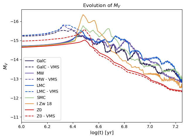
Figure 16: As described in Fig. 7 but showing M_V.

Appendix C Additional comparisons

For completeness we include here a number of comparisons between Starburst99 and pyStarburst99, such as the SEDs with similar inputs from both code versions, the SEDs produced using WMbasic and Fastwind, and the SEDs including VMS at various metallicities.

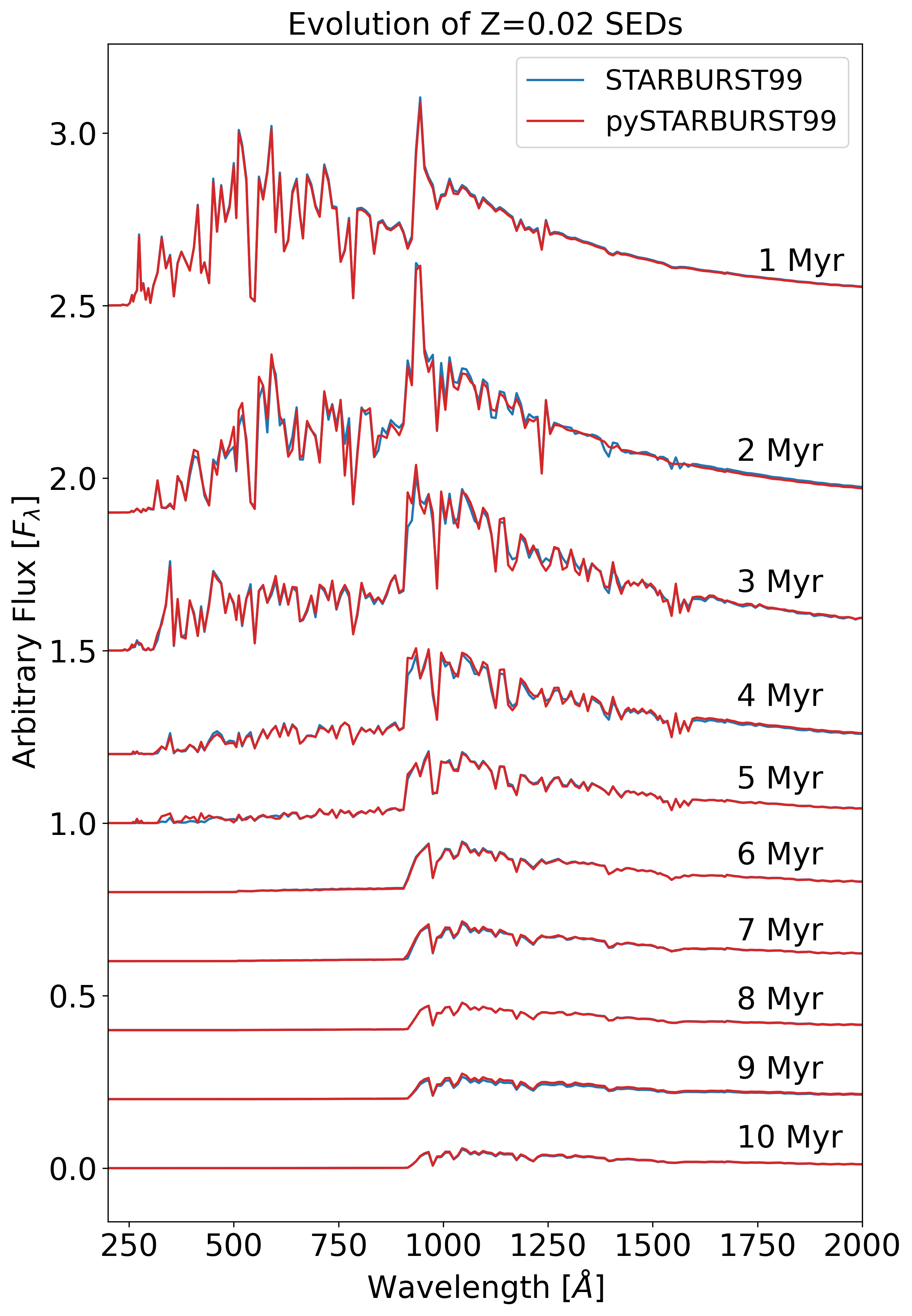
Figure 17: Synthetic FUV SEDs from Starburst99  compared to those produced with pyStarburst99, in both cases utilising the Yusof et al. (2022) stellar evolutionary models at $Z=0.02$ and WMbasic  spectra at $Z=0.02$. The evolution with time is shown from 1 Myr to 10 Myr at intervals of 1 Myr.

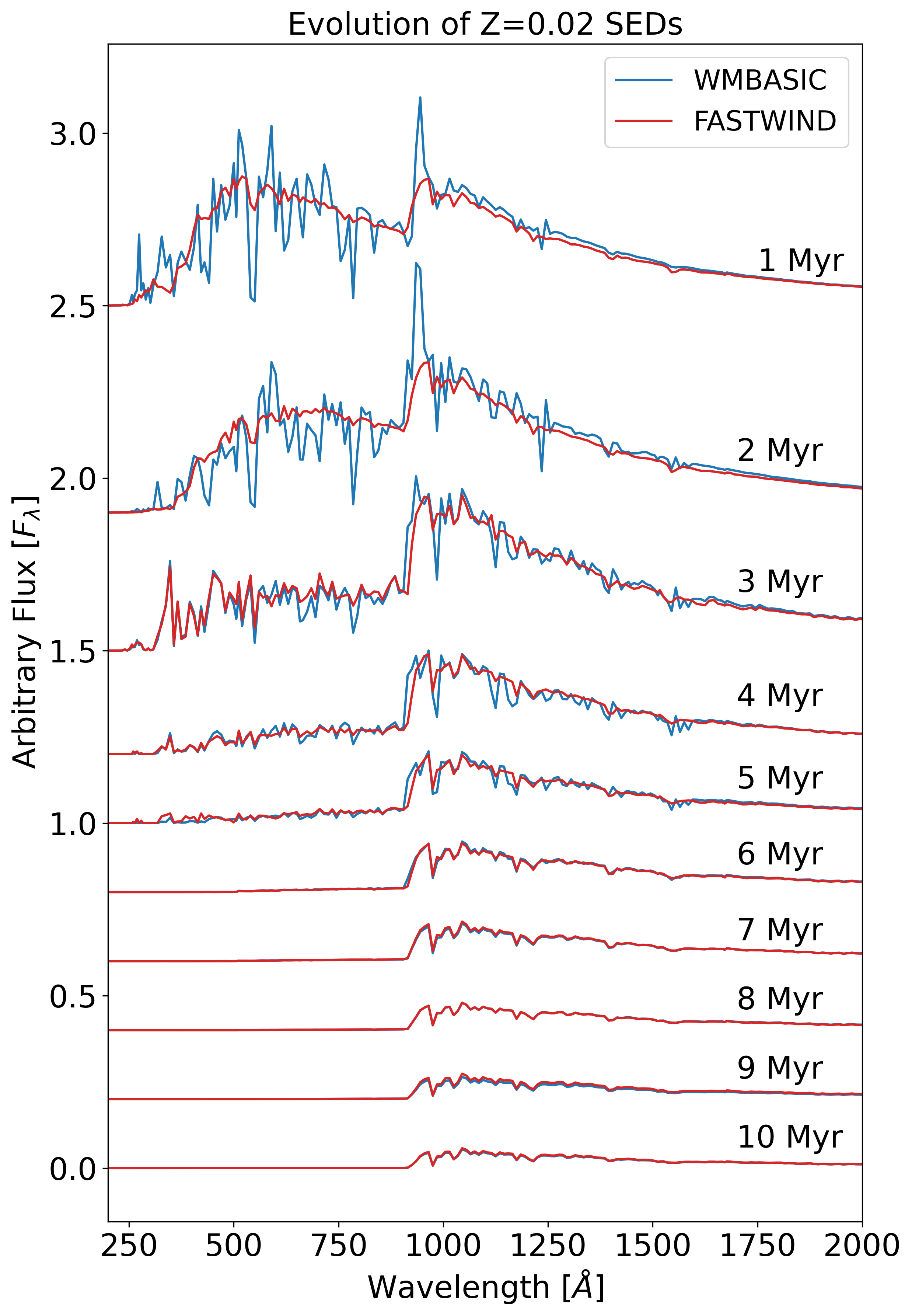
Figure 18: Synthetic FUV SEDs, utilising the Yusof et al. (2022) stellar evolutionary models at $Z=0.02$ for both, with WMbasic  spectra at $Z=0.02$ compared with Fastwind  spectra at $Z=0.02$. The evolution with time is shown from 1 Myr to 10 Myr at intervals of 1 Myr.

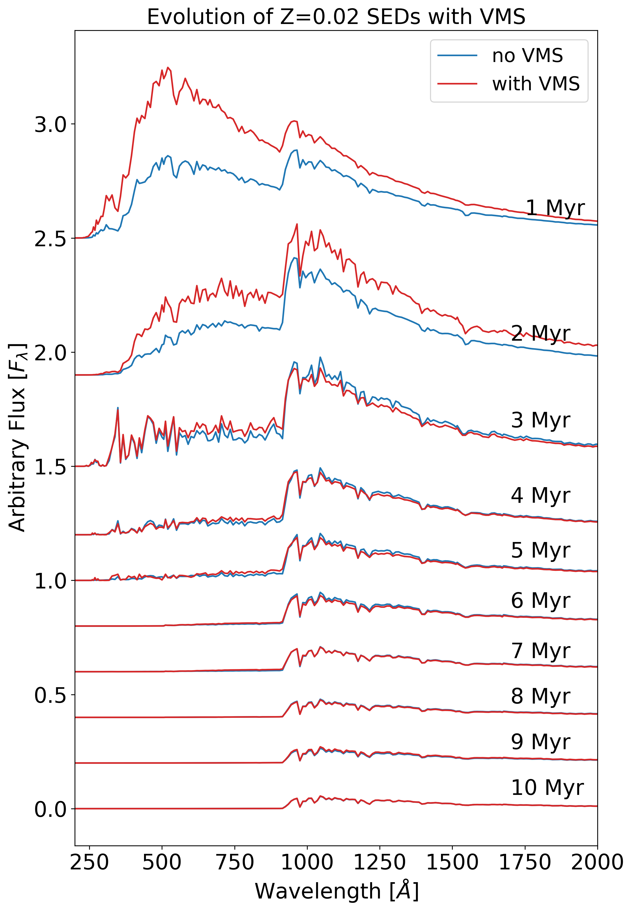
Figure 19: Synthetic FUV SEDs from pyStarburst99, utilising the Yusof et al. (2022) stellar evolutionary models at Z=0.02 and Fastwind  spectra at Z=0.02. This is compared with the addition of VMS evolutionary tracks up to $300M_{\odot}$ from Martinet et al. (2023) and Fastwind  models tailored to match the extended parameter space coverage from VMS evolutionary tracks. The evolution with time is shown from 1 Myr to 10 Myr at intervals of 1 Myr.

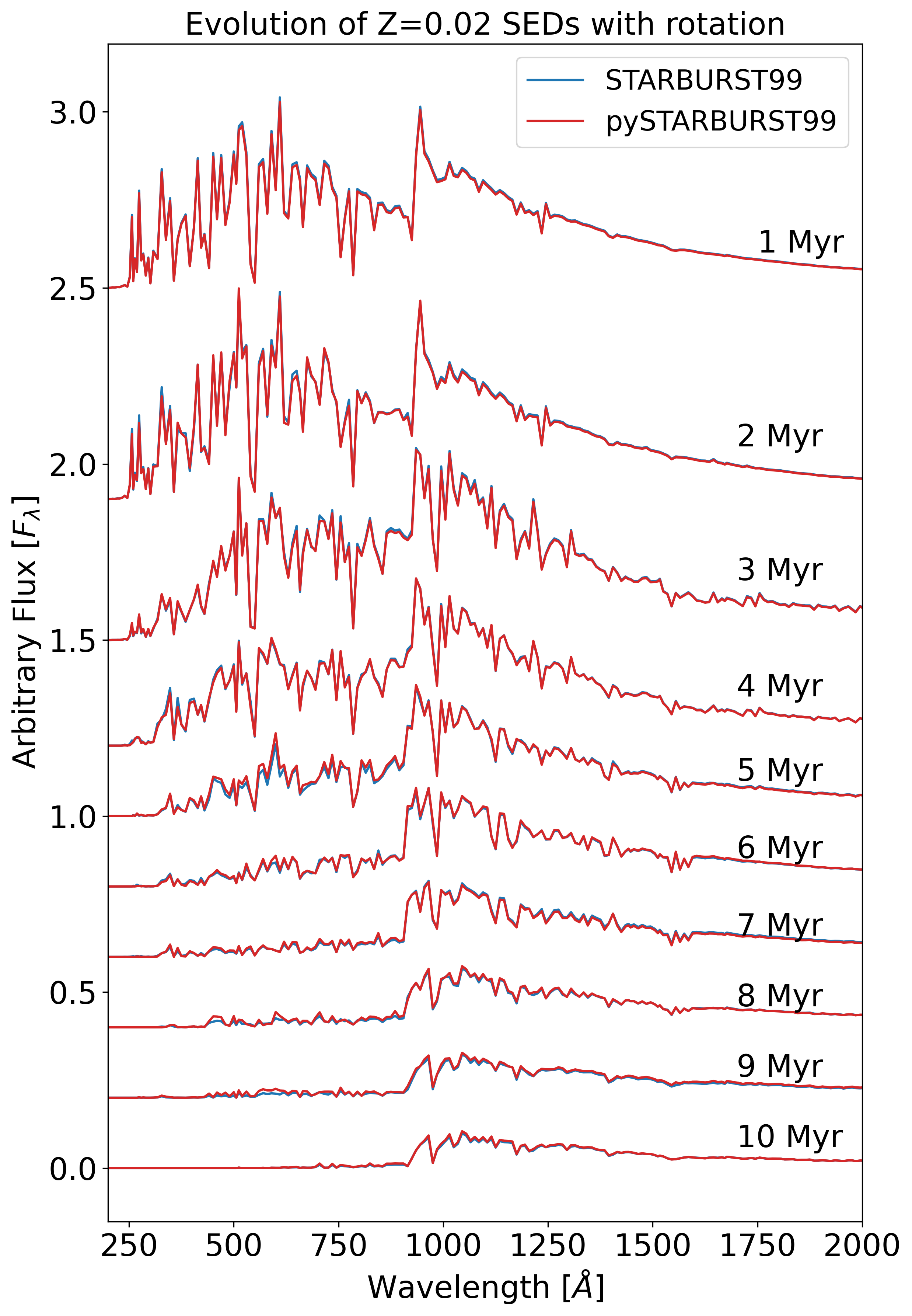
Figure 20: Synthetic FUV SEDs from Starburst99  compared to those produced with pyStarburst99, in both cases utilising the Yusof et al. (2022) stellar evolutionary models including rotation at $Z=0.02$ and WMbasic  spectra at $Z=0.02$. The evolution with time is shown from 1 Myr to 10 Myr at intervals of 1 Myr.

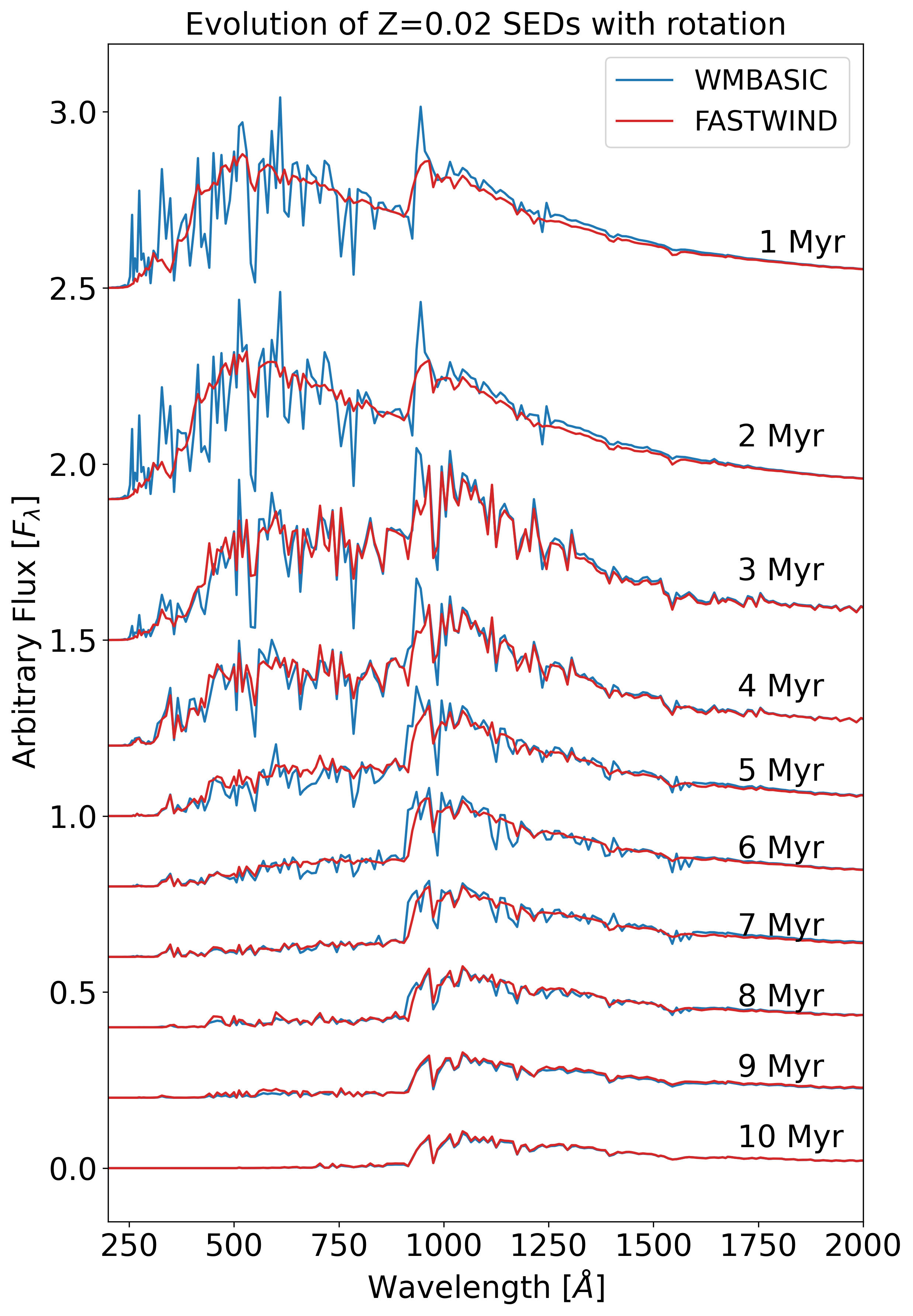
Figure 21: Synthetic FUV SEDs, utilising the Yusof et al. (2022) stellar evolutionary models at $Z=0.02$ with rotation for both, with WMbasic  spectra at $Z=0.02$ compared with Fastwind  spectra at $Z=0.02$. The evolution with time is shown from 1 Myr to 10 Myr at intervals of 1 Myr.

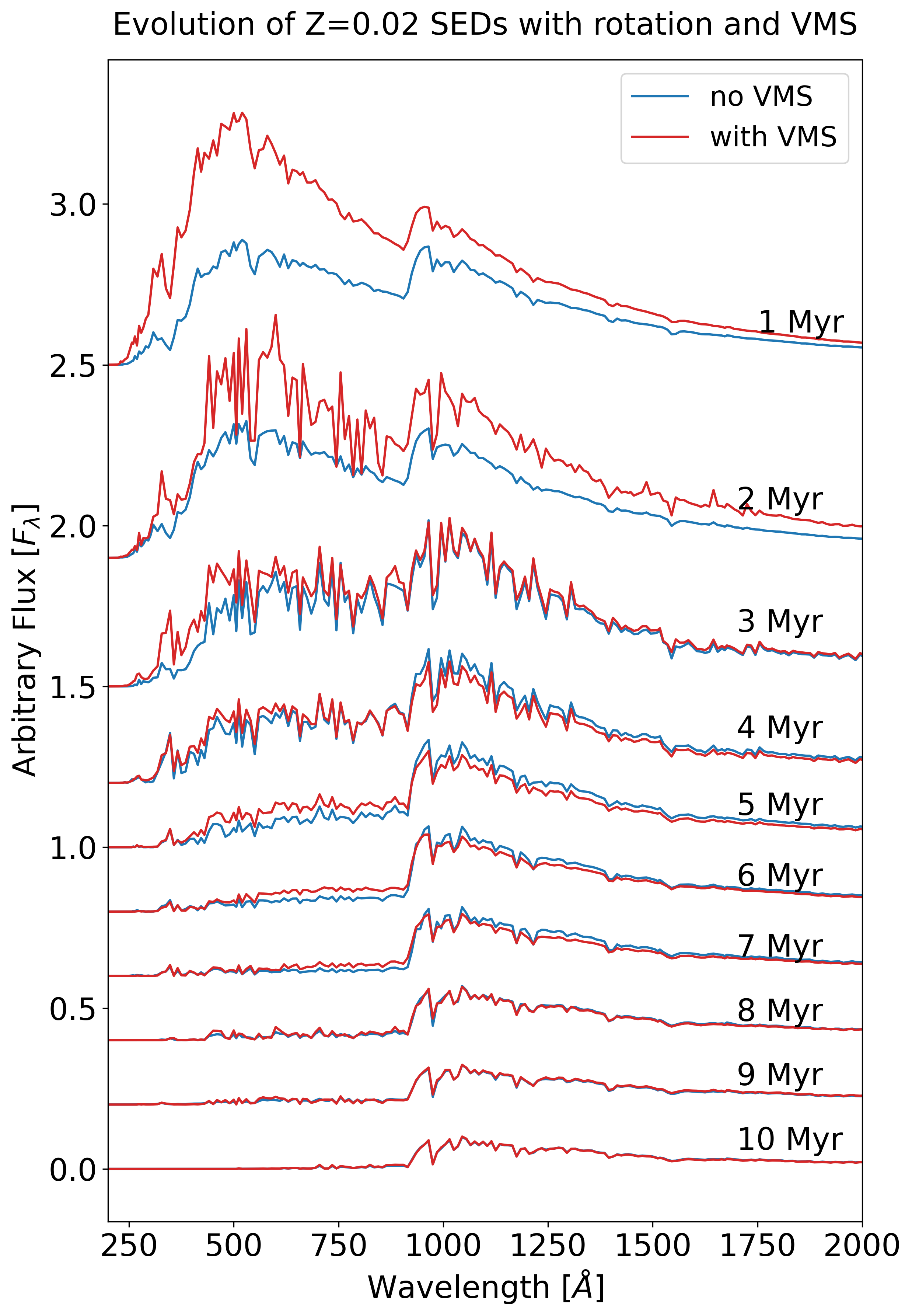
Figure 22: Synthetic FUV SEDs from pyStarburst99, utilising the Yusof et al. (2022) stellar evolutionary models at Z=0.02 with rotation and Fastwind  spectra at Z=0.02. This is compared with the addition of VMS evolutionary tracks up to $300M_{\odot}$ from Martinet et al. (2023) and Fastwind  models tailored to match the extended parameter space coverage from VMS evolutionary tracks. The evolution with time is shown from 1 Myr to 10 Myr at intervals of 1 Myr.

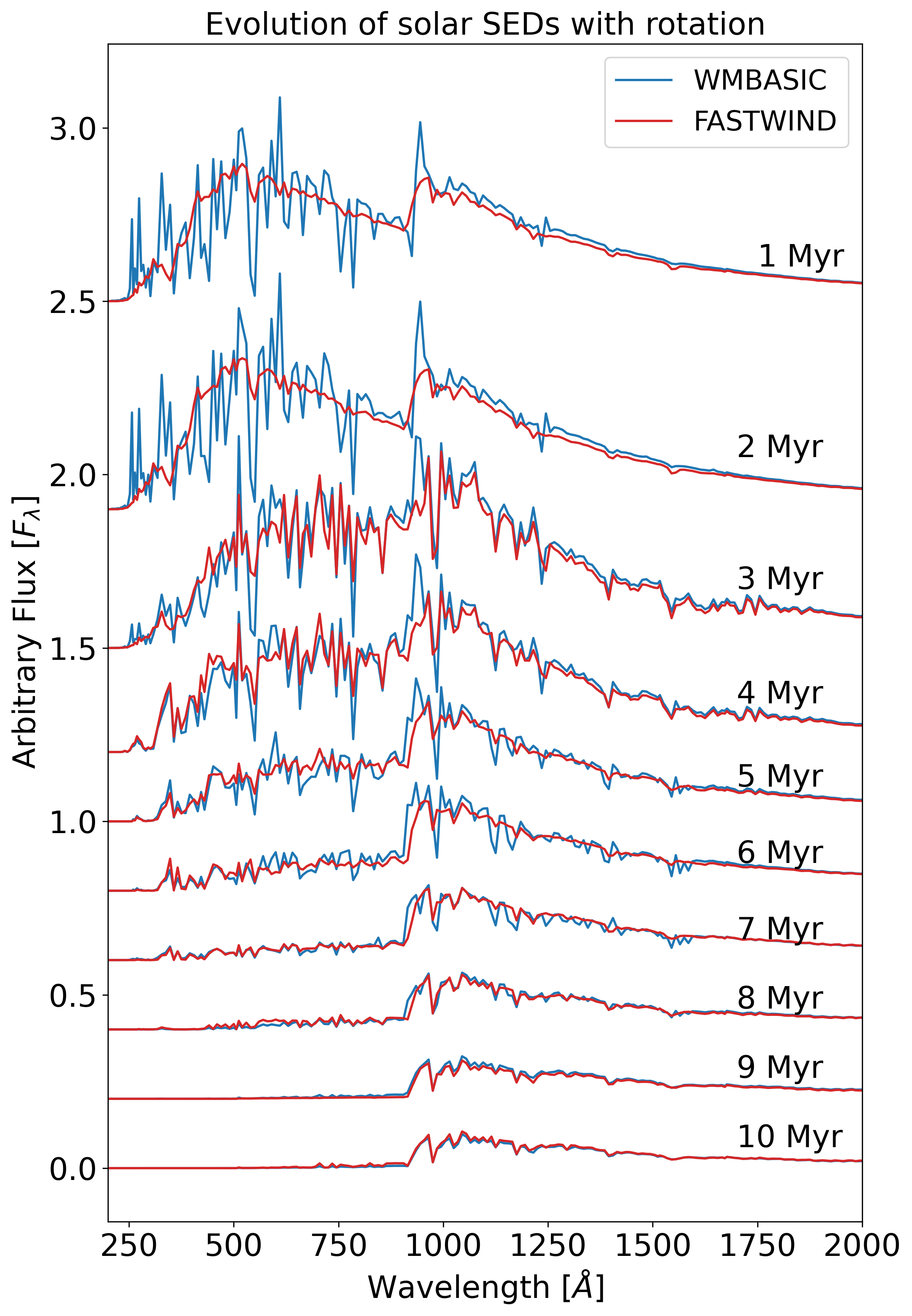
Figure 24: Synthetic FUV SEDs, utilising the Ekström et al. (2012) stellar evolutionary models at $Z=0.014$ with rotation for both, with WMbasic  spectra at $Z=0.02$ compared with Fastwind  spectra at $Z=0.014$. The evolution with time is shown from 1 Myr to 10 Myr at intervals of 1 Myr.

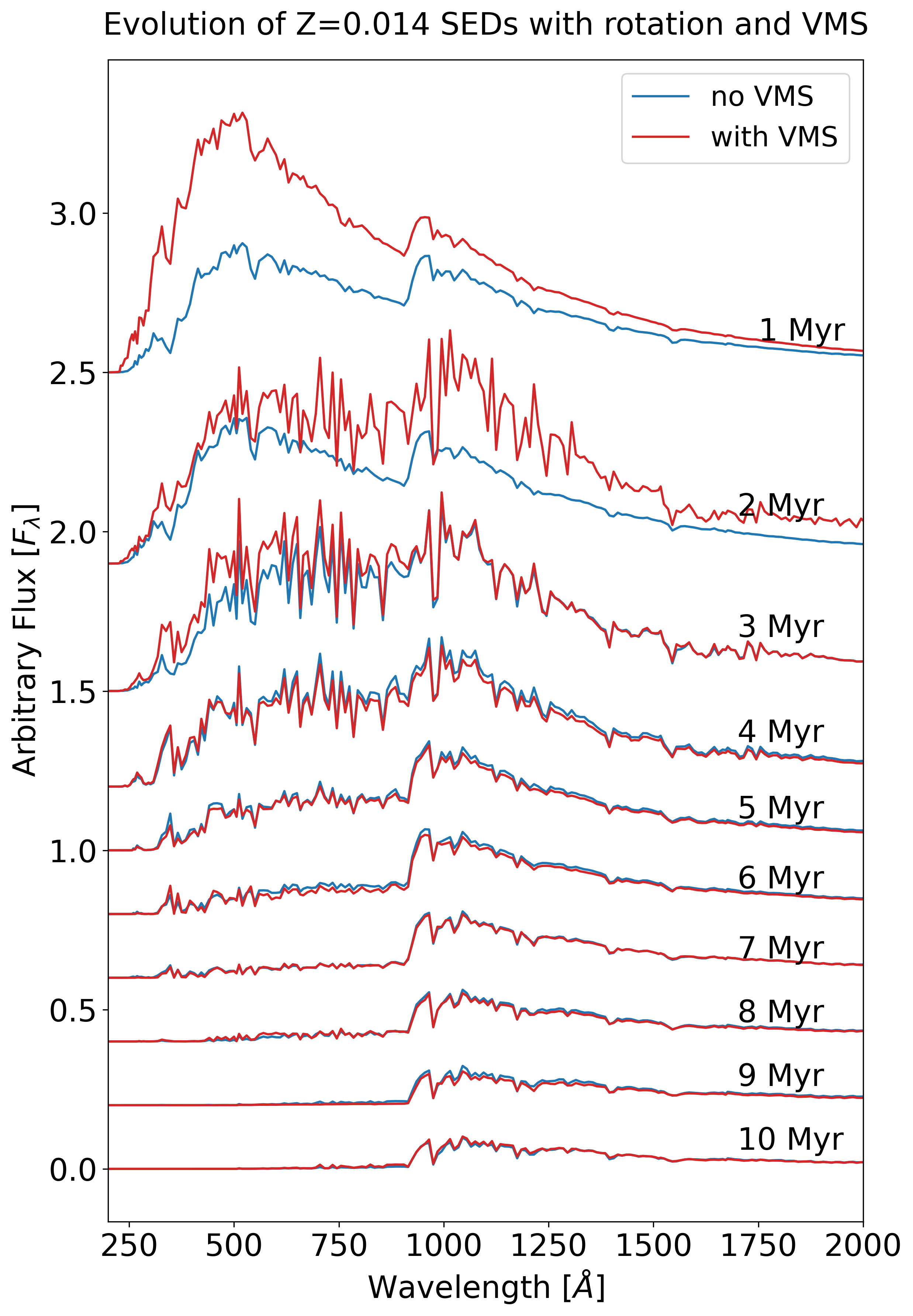
Figure 25: Synthetic FUV SEDs from pyStarburst99, utilising the Ekström et al. (2012) stellar evolutionary models at Z=0.014 with rotation and Fastwind  spectra at Z=0.014. This is compared with the addition of VMS evolutionary tracks up to $300M_{\odot}$ from Martinet et al. (2023) and Fastwind  models tailored to match the extended parameter space coverage from VMS evolutionary tracks. The evolution with time is shown from 1 Myr to 10 Myr at intervals of 1 Myr.

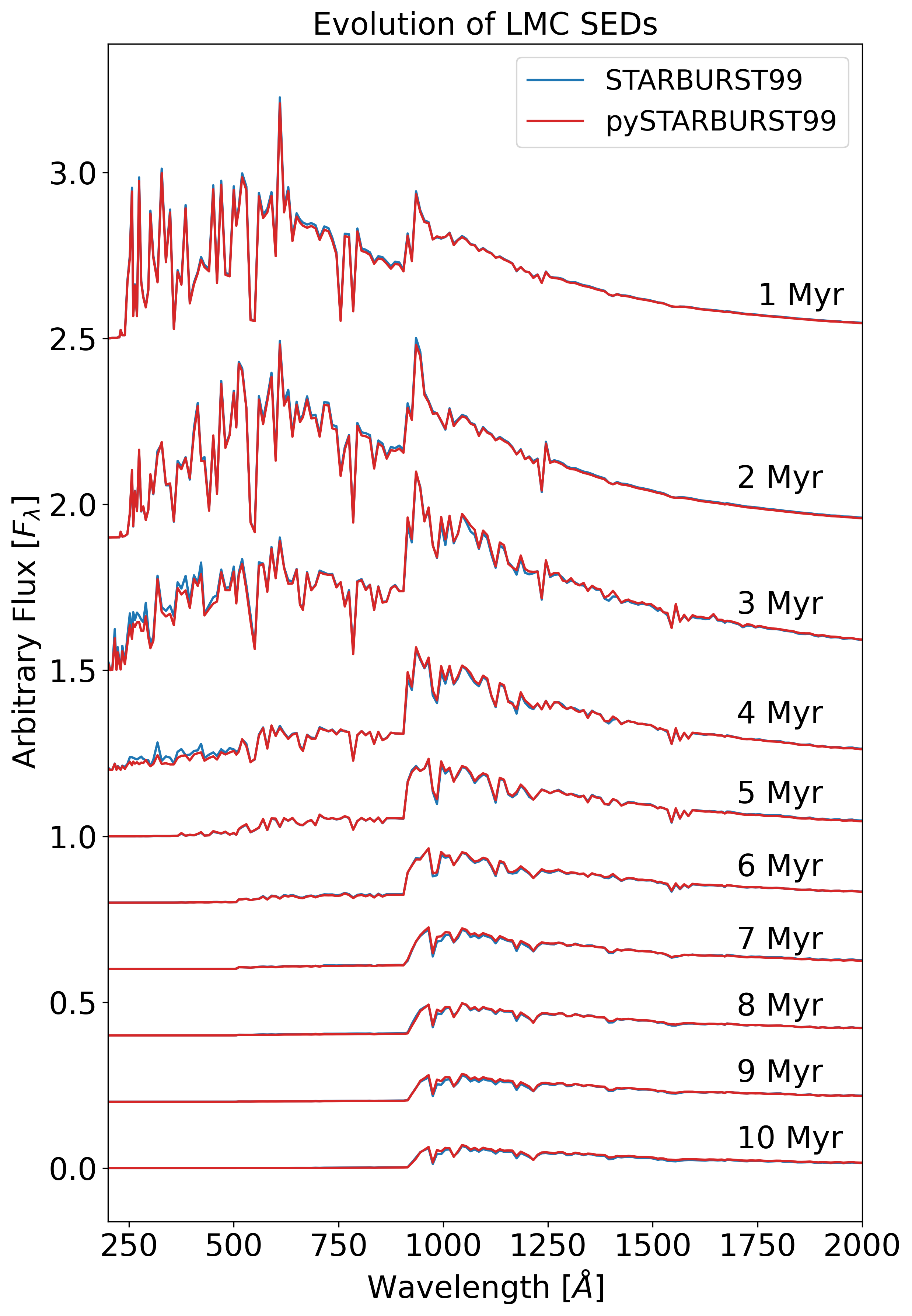
Figure 26: Synthetic FUV SEDs from Starburst99  compared to those produced with pyStarburst99, in both cases utilising the Eggenberger et al. (2021) stellar evolutionary models at Z=0.006 and WMbasic  spectra at Z=0.008. The evolution with time is shown from 1 Myr to 10 Myr at intervals of 1 Myr.

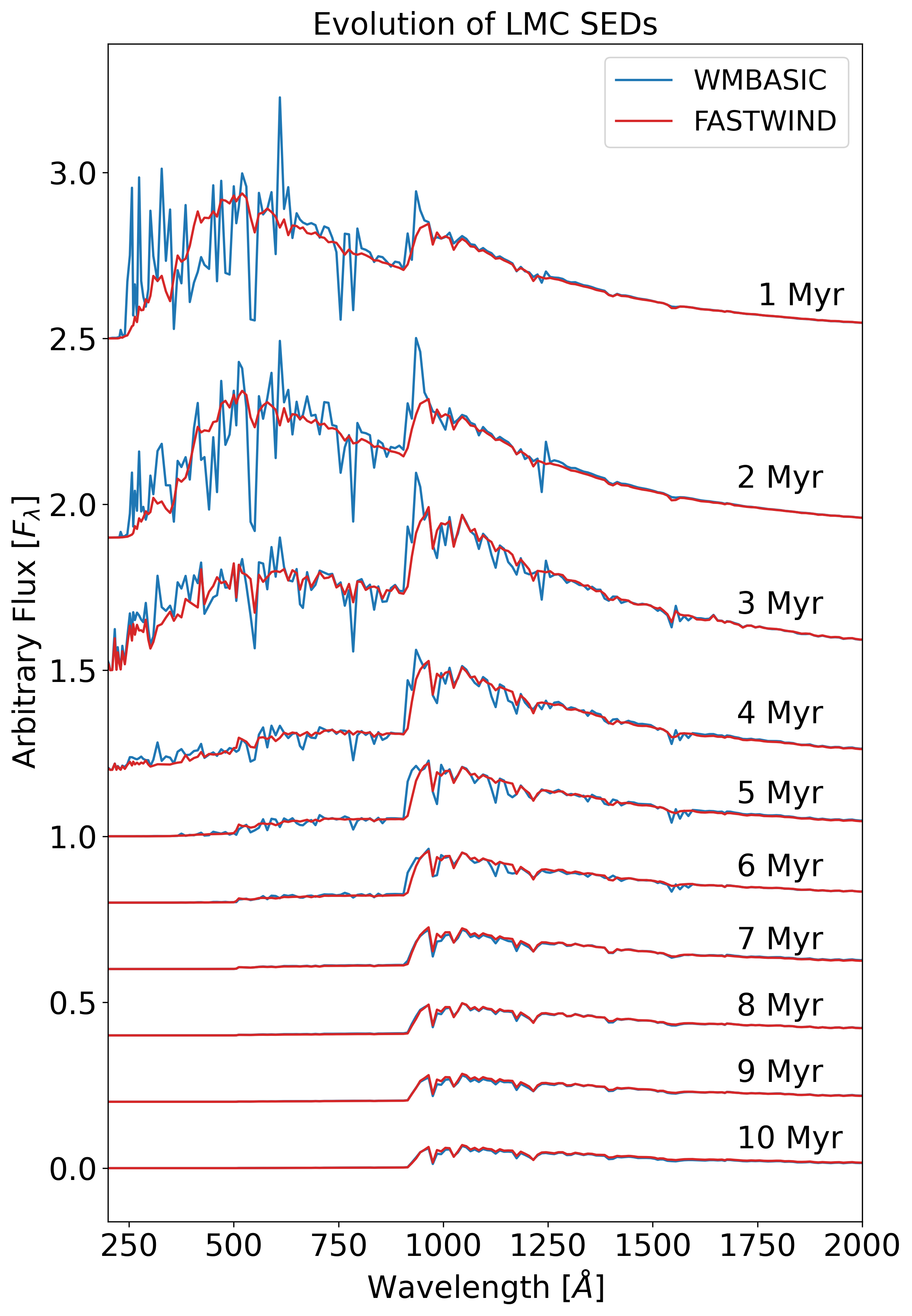
Figure 27: Synthetic FUV SEDs, utilising the Eggenberger et al. (2021) stellar evolutionary models at $Z=0.006$ for both, with WMbasic  spectra at $Z=0.008$ compared with Fastwind  spectra at $Z=0.006$. The evolution with time is shown from 1 Myr to 10 Myr at intervals of 1 Myr.

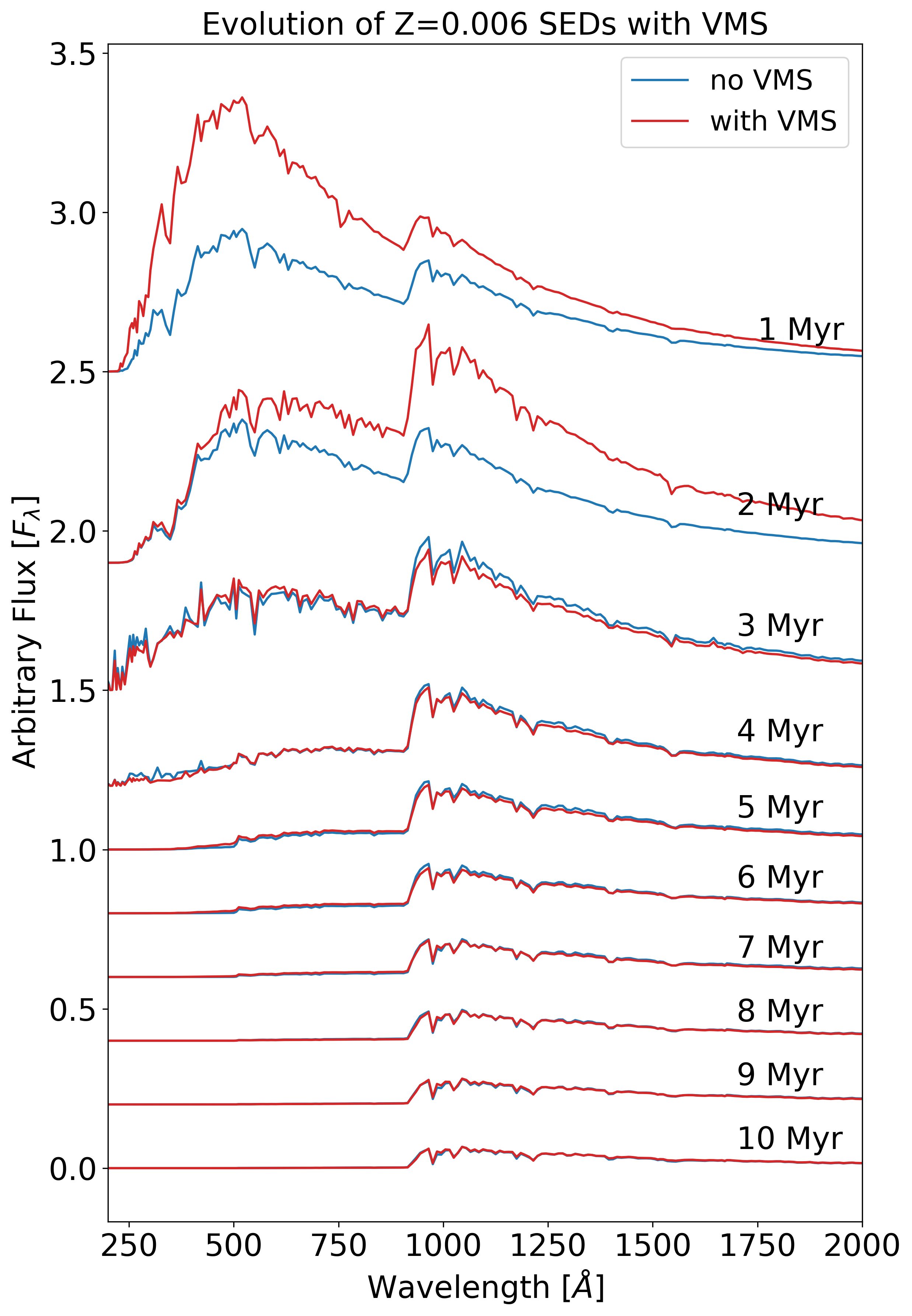
Figure 28: Synthetic FUV SEDs from pyStarburst99, utilising the Eggenberger et al. (2021) stellar evolutionary models at $Z=0.006$ and Fastwind  spectra at $Z=0.006$. This is compared with the addition of VMS evolutionary tracks up to $300M_{\odot}$ from Martinet et al. (2023) and Fastwind  models tailored to match the extended parameter space coverage from VMS evolutionary tracks. The evolution with time is shown from 1 Myr to 10 Myr at intervals of 1 Myr.

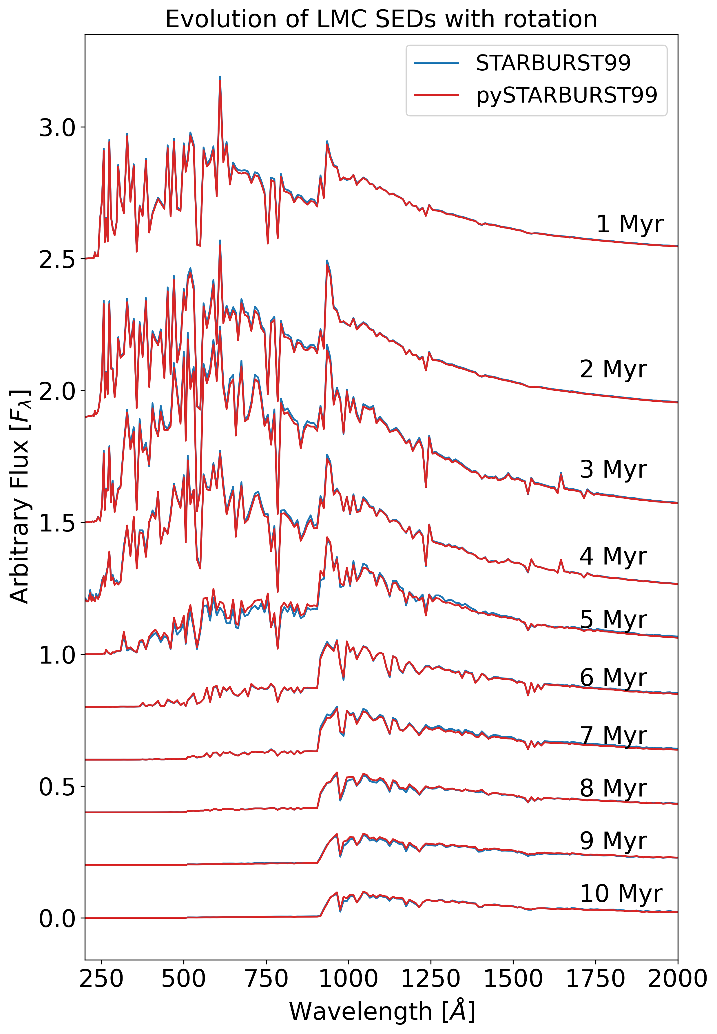
Figure 29: Synthetic FUV SEDs from Starburst99  compared to those produced with pyStarburst99, in both cases utilising the Eggenberger et al. (2021) stellar evolutionary models including rotation at $Z=0.006$ and WMbasic  spectra at $Z=0.008$. The evolution with time is shown from 1 Myr to 10 Myr at intervals of 1 Myr.

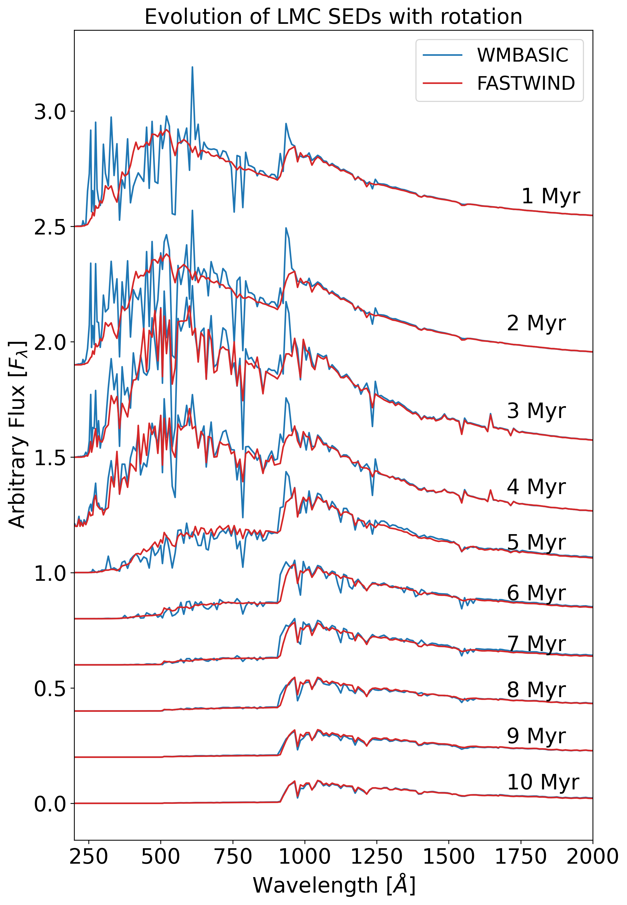
Figure 30: Synthetic FUV SEDs, utilising the Eggenberger et al. (2021) stellar evolutionary models at $Z=0.006$ with rotation for both, with WMbasic  spectra at $Z=0.008$ compared with Fastwind  spectra at $Z=0.006$. The evolution with time is shown from 1 Myr to 10 Myr at intervals of 1 Myr.

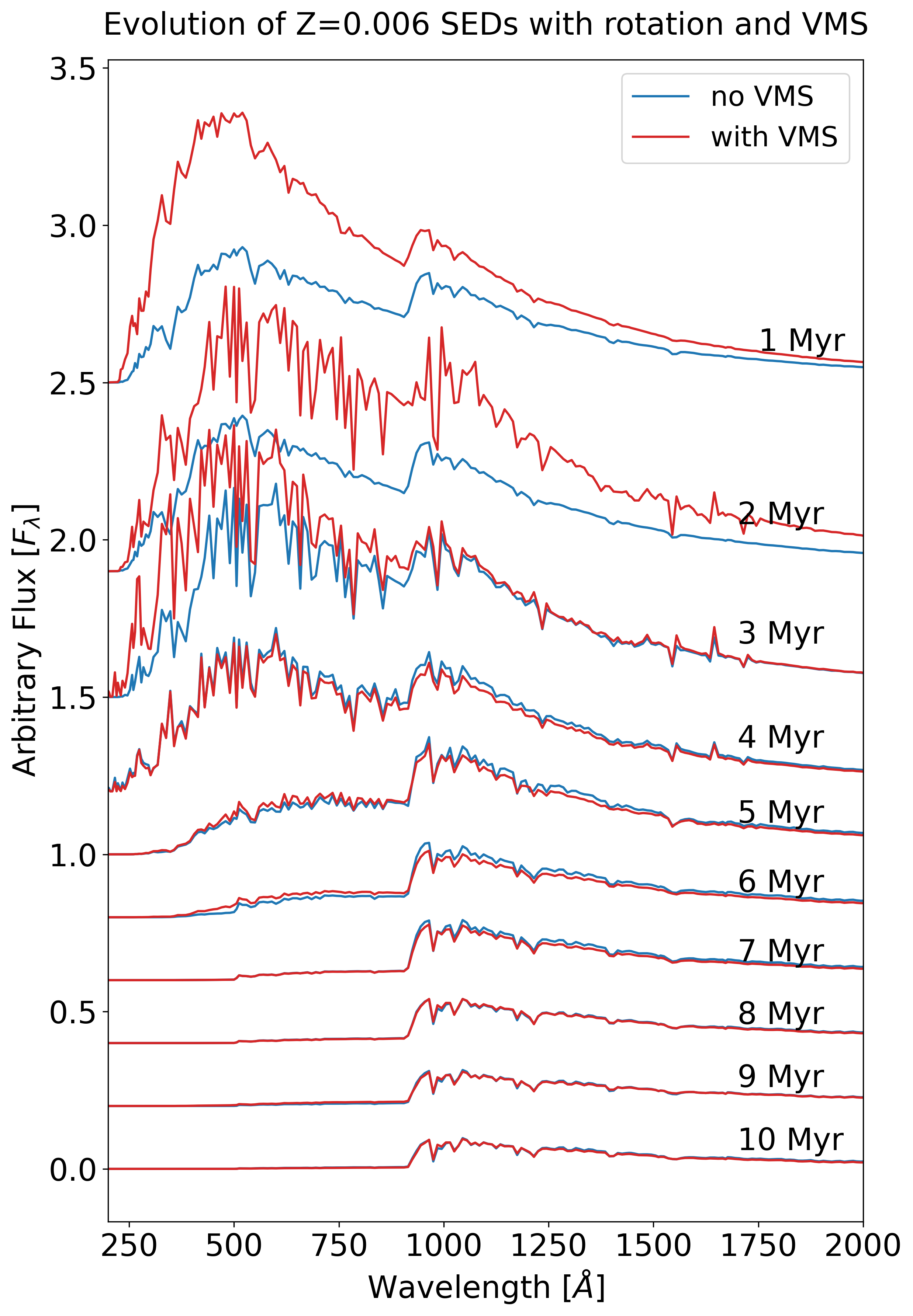
Figure 31: Synthetic FUV SEDs from pyStarburst99, utilising the Eggenberger et al. (2021) stellar evolutionary models at $Z=0.006$ with rotation and Fastwind  spectra at $Z=0.006$. This is compared with the addition of VMS evolutionary tracks up to $300M_{\odot}$ from Martinet et al. (2023) and Fastwind  models tailored to match the extended parameter space coverage from VMS evolutionary tracks. The evolution with time is shown from 1 Myr to 10 Myr at intervals of 1 Myr.

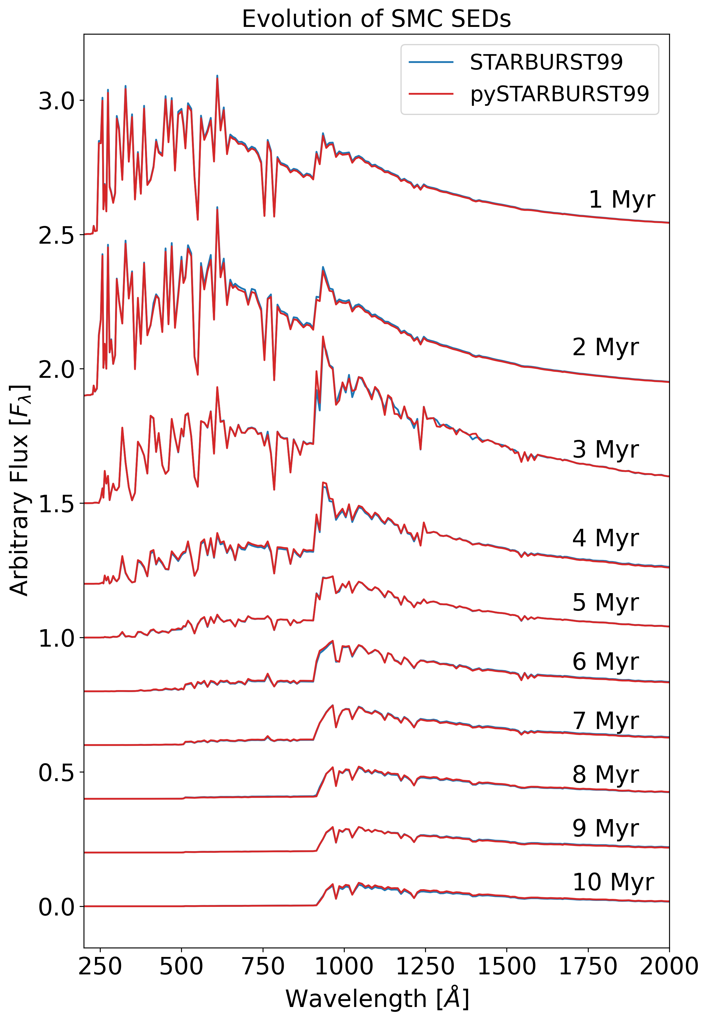
Figure 32: Synthetic FUV SEDs from Starburst99  compared to those produced with pyStarburst99, in both cases utilising the Georgy et al. (2013) stellar evolutionary models at $Z=0.002$ and WMbasic  spectra at $Z=0.004$. The evolution with time is shown from 1 Myr to 10 Myr at intervals of 1 Myr.

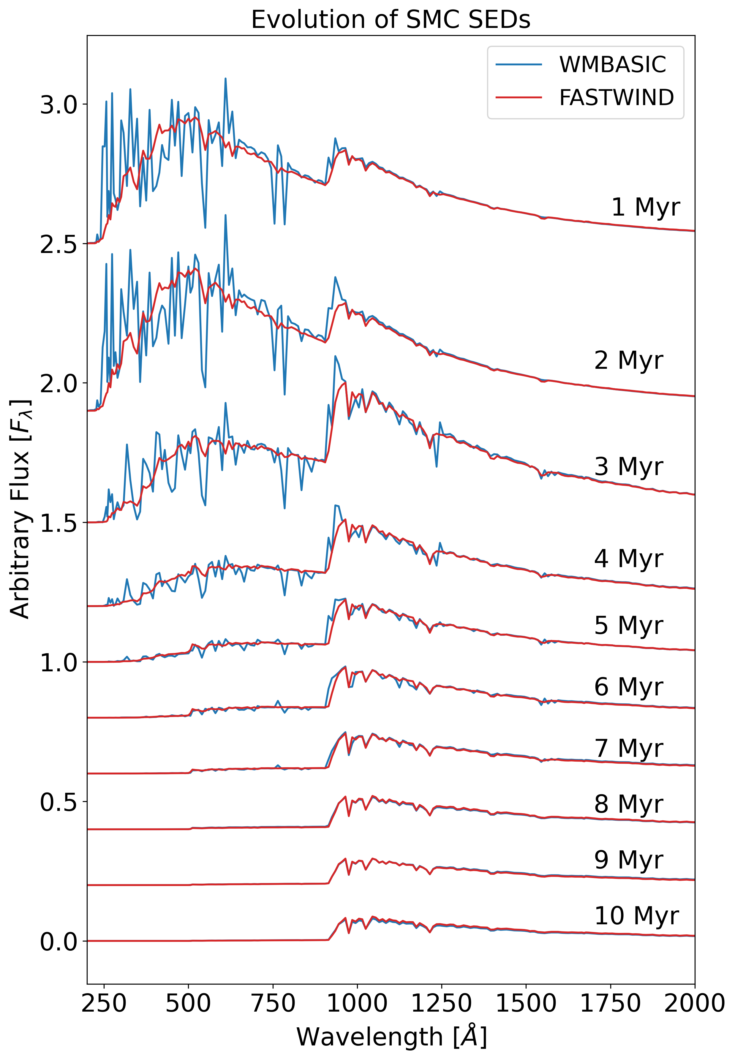
Figure 33: Synthetic FUV SEDs, utilising the Georgy et al. (2013) stellar evolutionary models at $Z=0.002$ for both, with WMbasic  spectra at $Z=0.004$ compared with Fastwind  spectra at $Z=0.002$. The evolution with time is shown from 1 Myr to 10 Myr at intervals of 1 Myr.

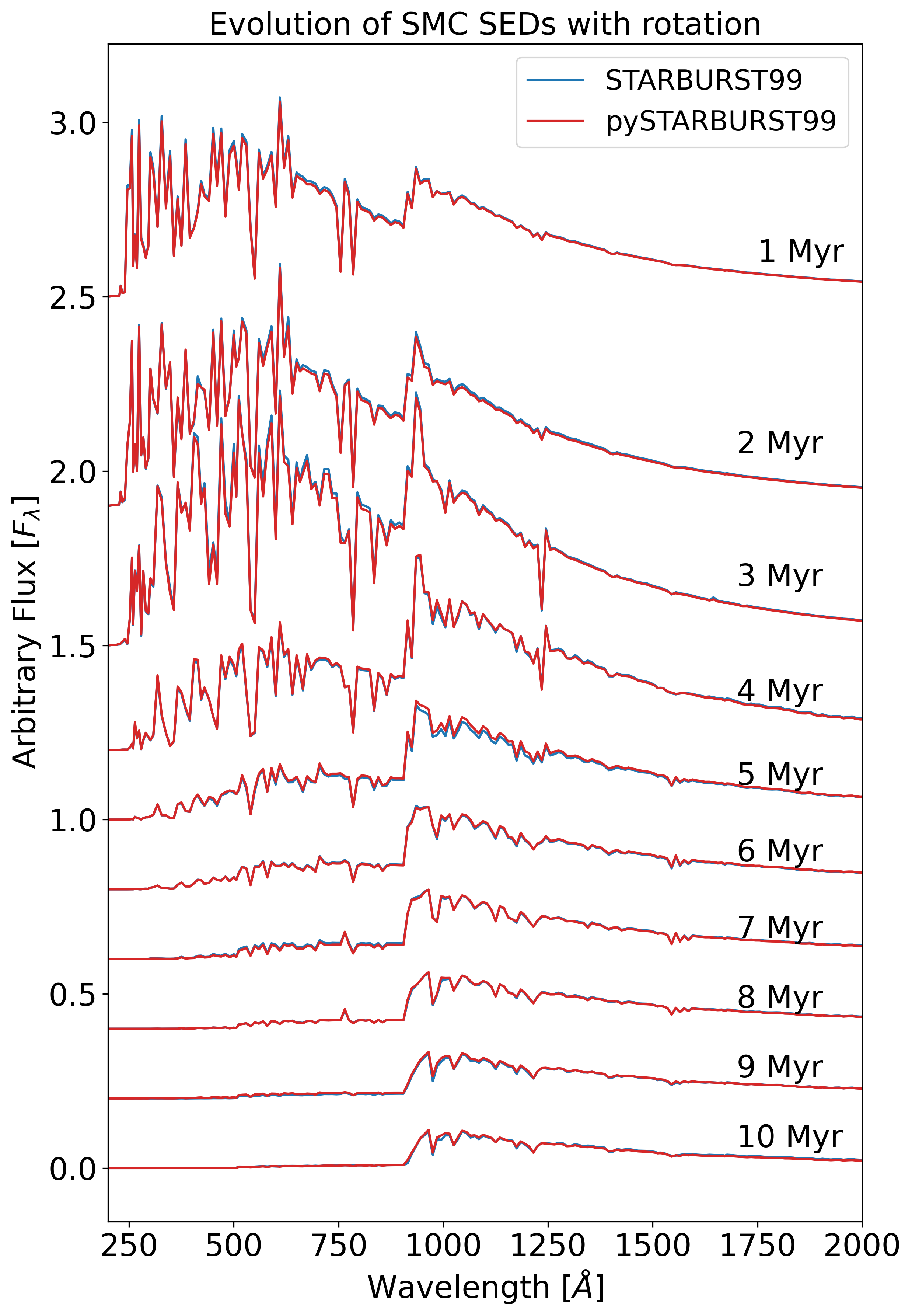
Figure 34: Synthetic FUV SEDs from Starburst99  compared to those produced with pyStarburst99, in both cases utilising the Georgy et al. (2013) stellar evolutionary models at $Z=0.002$ with rotation and WMbasic  spectra at $Z=0.004$. The evolution with time is shown from 1 Myr to 10 Myr at intervals of 1 Myr.

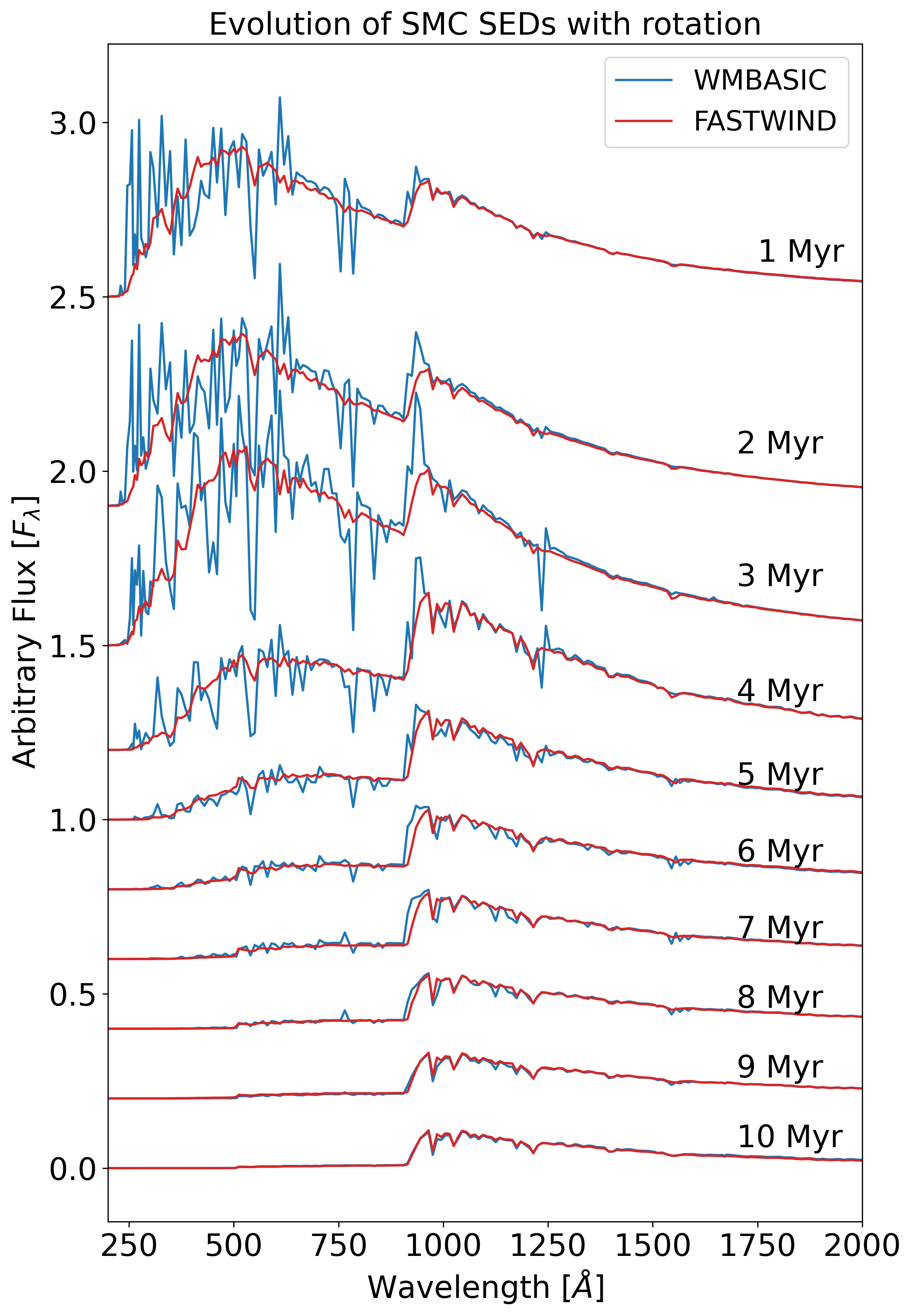
Figure 35: Synthetic FUV SEDs, utilising the Georgy et al. (2013) stellar evolutionary models at $Z=0.002$ with rotation for both, with WMbasic  spectra at $Z=0.004$ compared with Fastwind  spectra at $Z=0.002$. The evolution with time is shown from 1 Myr to 10 Myr at intervals of 1 Myr.

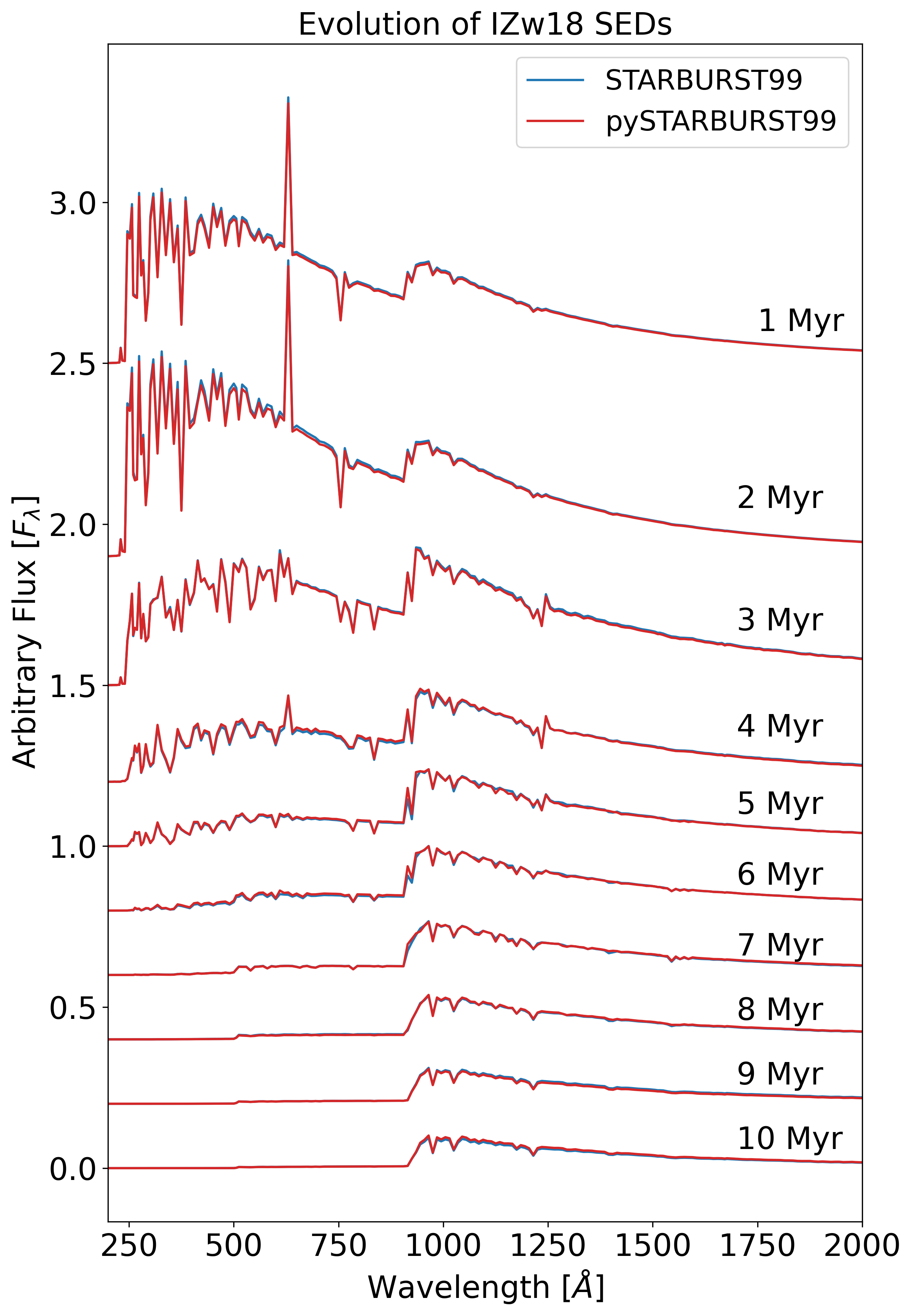
Figure 36: Synthetic FUV SEDs from Starburst99  compared to those produced with pyStarburst99, in both cases utilising the Groh et al. (2019) stellar evolutionary models at $Z=0.0004$ and WMbasic  spectra at $Z=0.001$. The evolution with time is shown from 1 Myr to 10 Myr at intervals of 1 Myr.

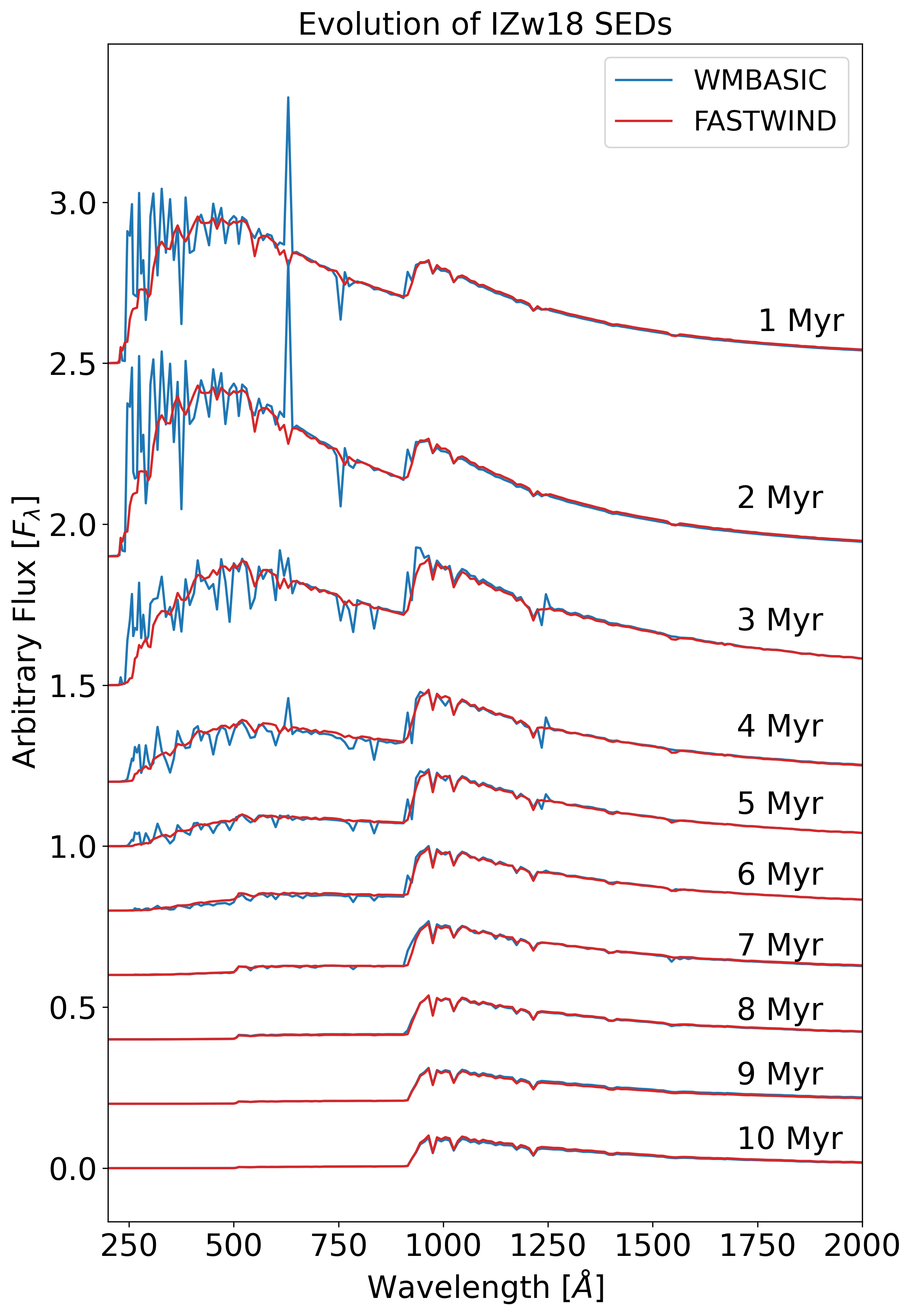
Figure 37: Synthetic FUV SEDs, utilising the Groh et al. (2019) stellar evolutionary models at $Z=0.0004$ for both, with WMbasic  spectra at $Z=0.001$ compared with Fastwind  spectra at $Z=0.004$. The evolution with time is shown from 1 Myr to 10 Myr at intervals of 1 Myr.

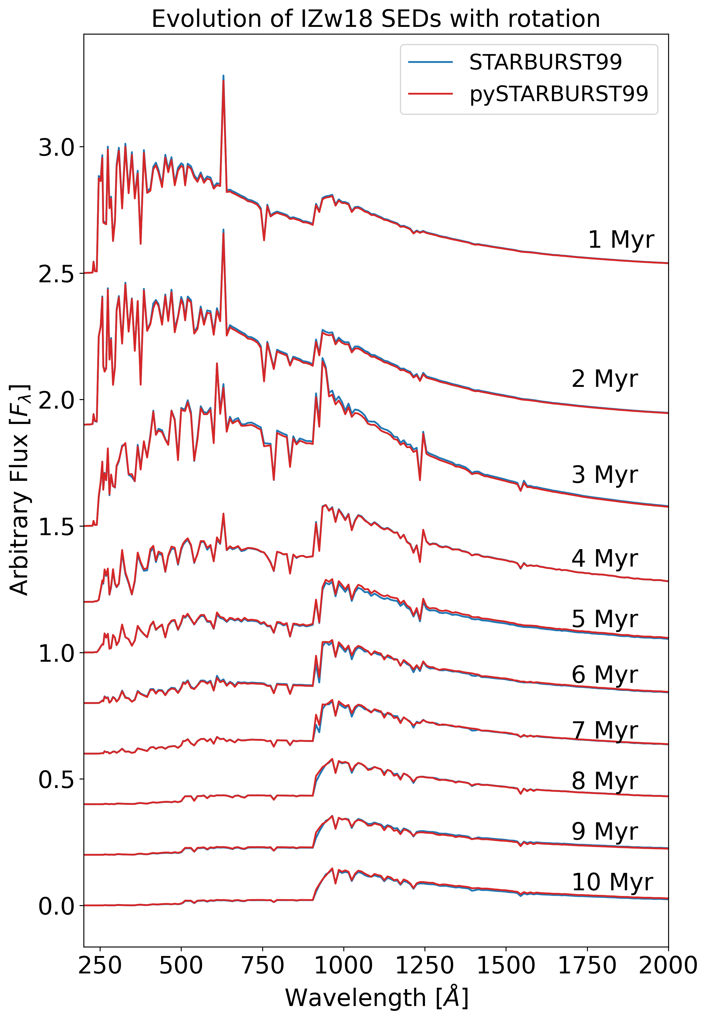
Figure 38: Synthetic FUV SEDs from Starburst99  compared to those produced with pyStarburst99, in both cases utilising the Groh et al. (2019) stellar evolutionary models at $Z=0.0004$ with rotation and WMbasic  spectra at $Z=0.001$. The evolution with time is shown from 1 Myr to 10 Myr at intervals of 1 Myr.

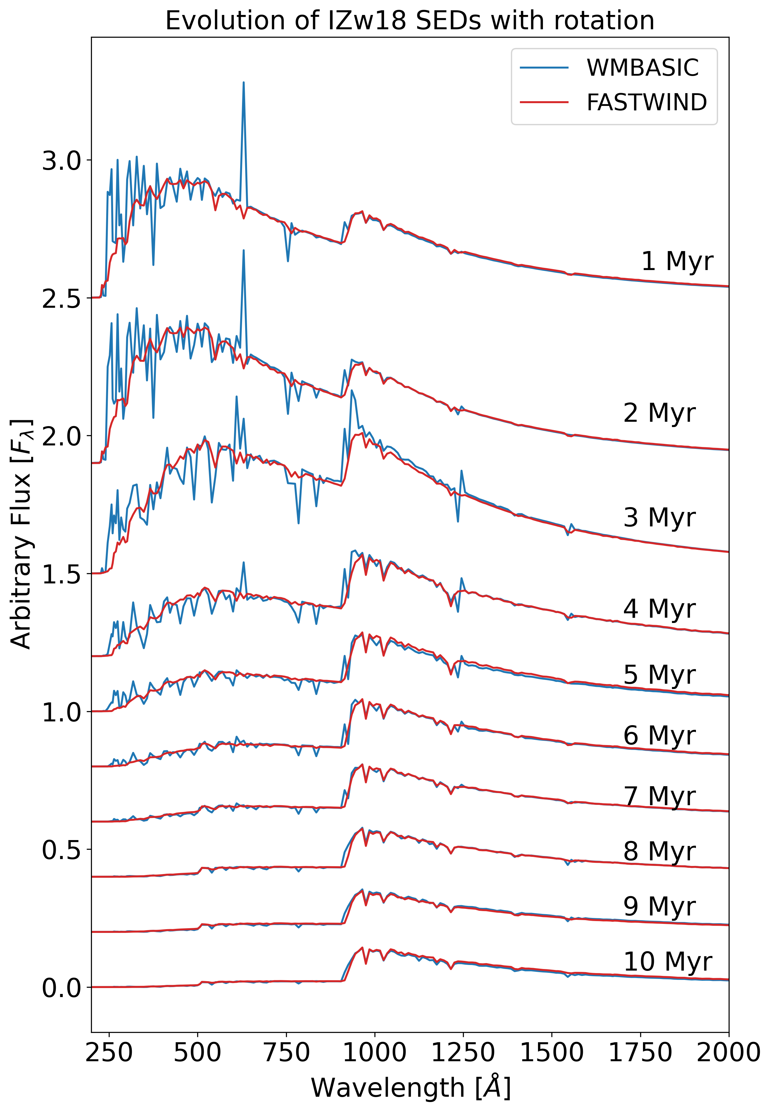
Figure 39: Synthetic FUV SEDs, utilising the Groh et al. (2019) stellar evolutionary models at $Z=0.0004$ with rotation for both, with WMbasic  spectra at $Z=0.001$ compared with Fastwind  spectra at $Z=0.004$. The evolution with time is shown from 1 Myr to 10 Myr at intervals of 1 Myr.

Figure 40: Synthetic FUV SEDs from Starburst99  compared to those produced with pyStarburst99, in both cases utilising the Murphy et al. (2021) stellar evolutionary models at $Z=0.0$ and WMbasic  spectra at $Z=0.001$. The evolution with time is shown from 1 Myr to 10 Myr at intervals of 1 Myr.

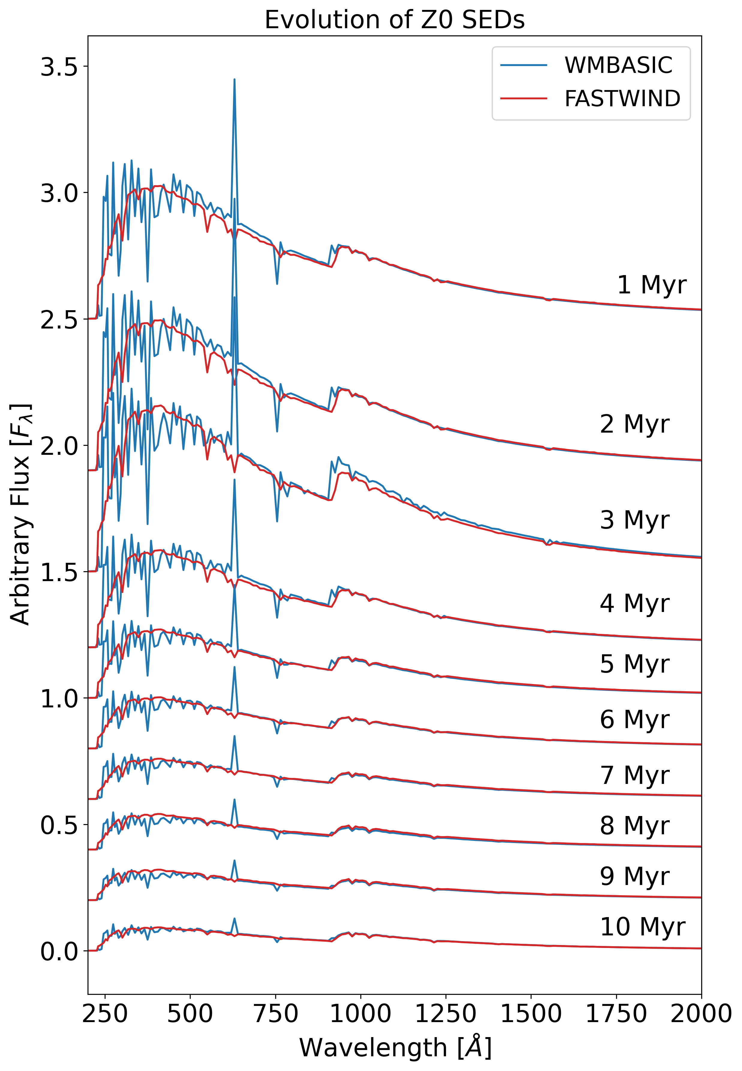
Figure 41: Synthetic FUV SEDs, utilising the Murphy et al. (2021) stellar evolutionary models at $Z=0.0$ for both, with WMbasic  spectra at $Z=0.001$ compared with Fastwind  spectra at $Z=1E-6$. The evolution with time is shown from 1 Myr to 10 Myr at intervals of 1 Myr.

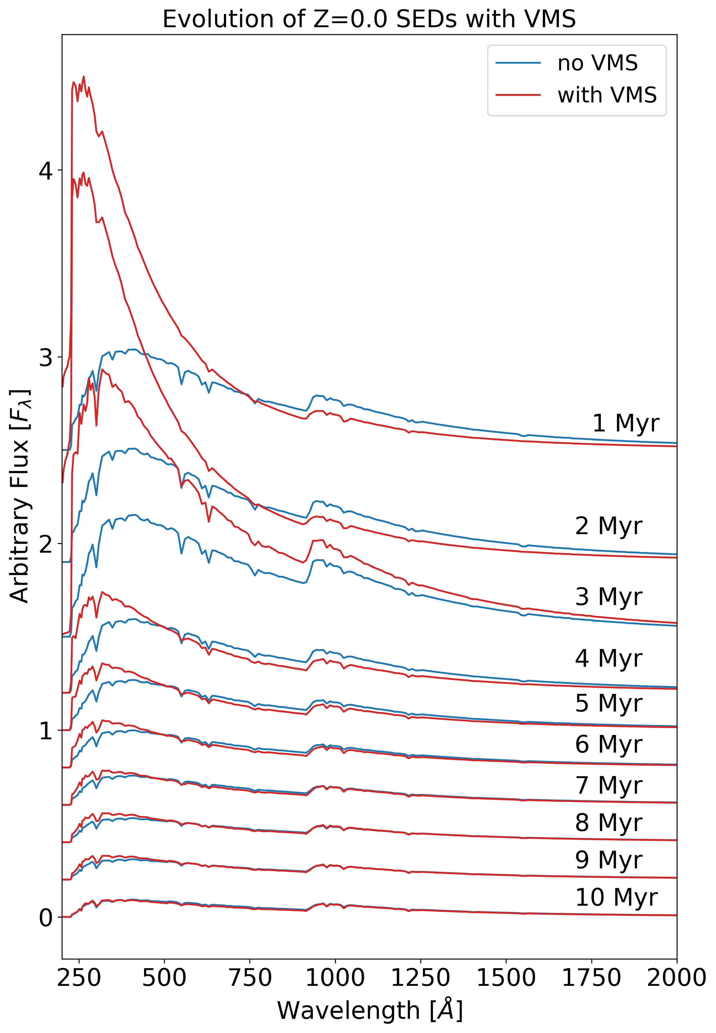
Figure 42: Synthetic FUV SEDs from pyStarburst99, utilising the Murphy et al. (2021) stellar evolutionary models at $Z=0.0$ and Fastwind  spectra at $Z=1E-6$. This is compared with the addition of VMS evolutionary tracks up to $300M_{\odot}$ from Martinet et al. (2023) and Fastwind  models tailored to match the extended parameter space coverage from VMS evolutionary tracks. The evolution with time is shown from 1 Myr to 10 Myr at intervals of 1 Myr.

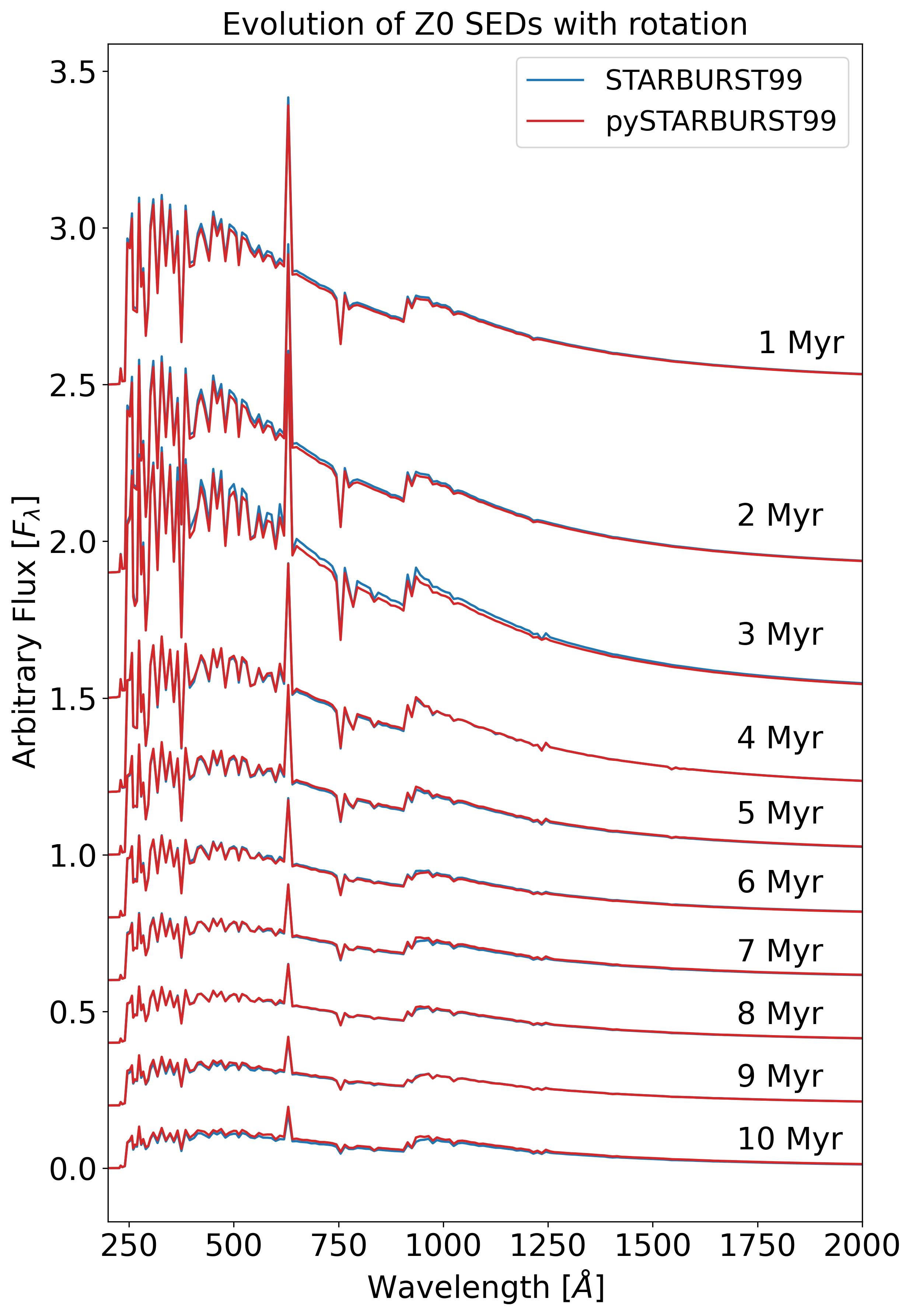
Figure 43: Synthetic FUV SEDs from Starburst99  compared to those produced with pyStarburst99, in both cases utilising the Murphy et al. (2021) stellar evolutionary models with rotation at Z=0.0 and WMbasic  spectra at $Z=0.001$. The evolution with time is shown from 1 Myr to 10 Myr at intervals of 1 Myr.

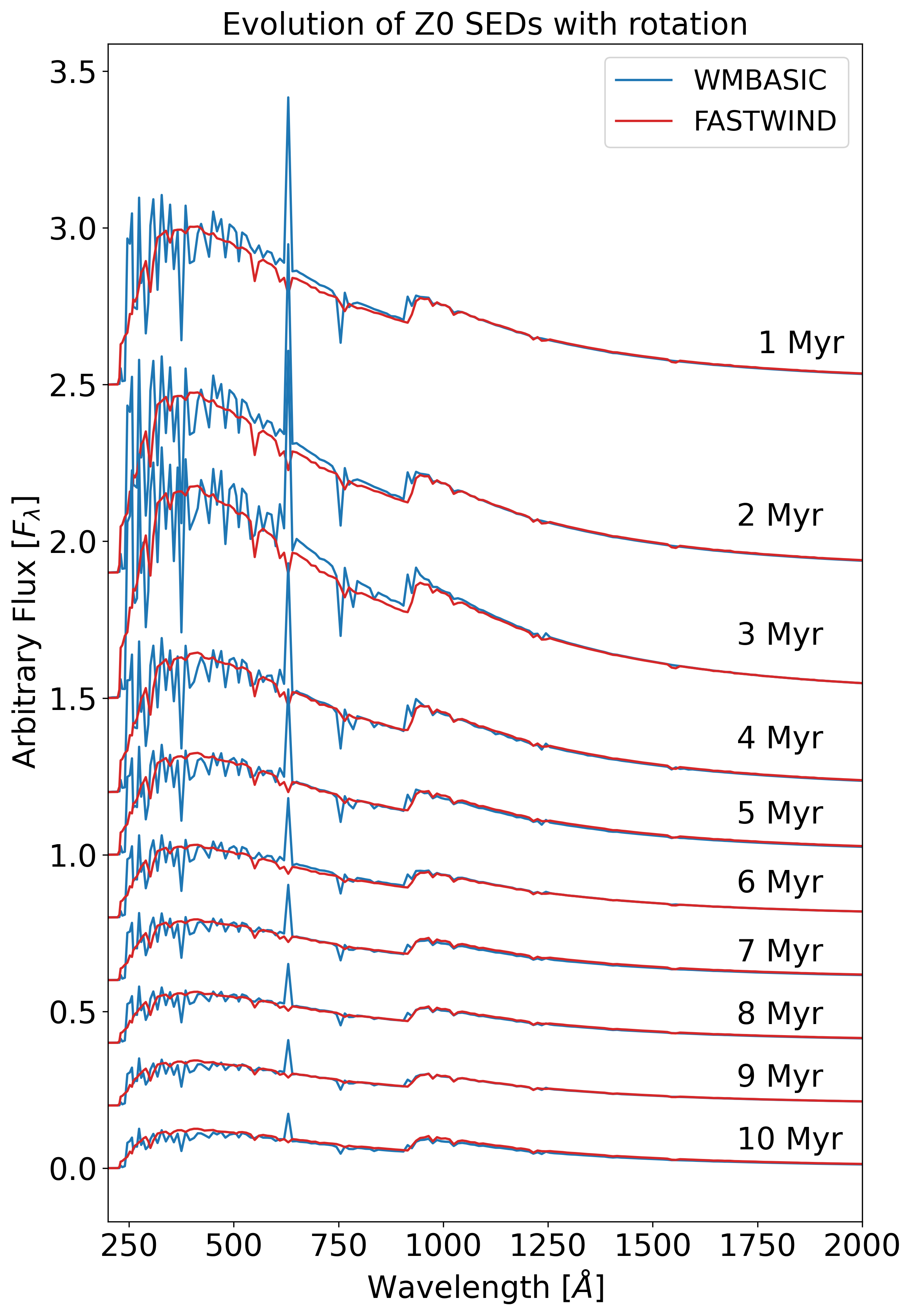
Figure 44: Synthetic FUV SEDs, utilising the Murphy et al. (2021) stellar evolutionary models with rotation at $Z=0.0$ for both, with WMbasic  spectra at $Z=0.001$ compared with Fastwind  spectra at $Z=1E-6$. The evolution with time is shown from 1 Myr to 10 Myr at intervals of 1 Myr.

References

- Agrawal et al. (2021) Agrawal, P., Hurley, J., Stevenson, S., Szécsi, D., & Flynn, C. 2021, in MOBSTER-1 virtual conference: Stellar Variability as a Probe of Magnetic Fields in Massive Stars, 22, doi: 10.5281/zenodo.5525465
- Asplund et al. (2009) Asplund, M., Grevesse, N., Sauval, A. J., & Scott, P. 2009, ARA&A, 47, 481, doi: 10.1146/annurev.astro.46.060407.145222
- Backs et al. (2024) Backs, F., Brands, S. A., de Koter, A., et al. 2024, arXiv e-prints, arXiv:2411.06884, doi: 10.48550/arXiv.2411.06884
- Berg et al. (2022) Berg, D. A., James, B. L., King, T., et al. 2022, ApJS, 261, 31, doi: 10.3847/1538-4365/ac6c03
- Berg et al. (2024) Berg, D. A., Skillman, E. D., Chisholm, J., et al. 2024, ApJ, 971, 87, doi: 10.3847/1538-4357/ad5292
- Bestenlehner et al. (2014) Bestenlehner, J. M., Gräfener, G., Vink, J. S., et al. 2014, The VLT-FLAMES tarantula survey: XVII. Physical and wind properties of massive stars at the top of the main sequence, EDP Sciences, doi: 10.1051/0004-6361/201423643
- Bestenlehner et al. (2020) Bestenlehner, J. M., Crowther, P. A., Caballero-Nieves, S. M., et al. 2020, MNRAS, 499, 1918, doi: 10.1093/mnras/staa2801
- Björklund et al. (2021) Björklund, R., Sundqvist, J. O., Puls, J., & Najarro, F. 2021, A&A, 648, A36, doi: 10.1051/0004-6361/202038384
- Boquien et al. (2019) Boquien, M., Burgarella, D., Roehlly, Y., et al. 2019, A&A, 622, A103, doi: 10.1051/0004-6361/201834156
- Bouret et al. (2015) Bouret, J. C., Lanz, T., Hillier, D. J., et al. 2015, MNRAS, 449, 1545, doi: 10.1093/mnras/stv379
- Brands et al. (2022) Brands, S. A., de Koter, A., Bestenlehner, J. M., et al. 2022, A&A, 663, A36, doi: 10.1051/0004-6361/202142742
- Broekgaarden et al. (2021) Broekgaarden, F. S., Berger, E., Neijssel, C. J., et al. 2021, MNRAS, 508, 5028, doi: 10.1093/mnras/stab2716
- Brott et al. (2011) Brott, I., de Mink, S. E., Cantiello, M., et al. 2011, A&A, 530, A115, doi: 10.1051/0004-6361/201016113
- Bruzual & Charlot (2003) Bruzual, G., & Charlot, S. 2003, MNRAS, 344, 1000, doi: 10.1046/j.1365-8711.2003.06897.x
- Byler et al. (2017) Byler, N., Dalcanton, J. J., Conroy, C., & Johnson, B. D. 2017, ApJ, 840, 44, doi: 10.3847/1538-4357/aa6c66
- Byrne et al. (2025) Byrne, C. M., Eldridge, J. J., & Stanway, E. R. 2025, MNRAS, 537, 2433, doi: 10.1093/mnras/staf178
- Calzetti et al. (1994) Calzetti, D., Kinney, A. L., & Storchi-Bergmann, T. 1994, ApJ, 429, 582, doi: 10.1086/174346
- Cameron et al. (2023) Cameron, A. J., Katz, H., Rey, M. P., & Saxena, A. 2023, MNRAS, 523, 3516, doi: 10.1093/mnras/stad1579
- Carneiro et al. (2016) Carneiro, L. P., Puls, J., Sundqvist, J. O., & Hoffmann, T. L. 2016, Astronomy and Astrophysics, 590, doi: 10.1051/0004-6361/201527718
- Chen et al. (2015) Chen, Y., Bressan, A., Girardi, L., et al. 2015, MNRAS, 452, 1068, doi: 10.1093/mnras/stv1281
- Chisholm et al. (2018) Chisholm, J., Gazagnes, S., Schaerer, D., et al. 2018, A&A, 616, A30, doi: 10.1051/0004-6361/201832758
- Choi et al. (2016) Choi, J., Dotter, A., Conroy, C., et al. 2016, ApJ, 823, 102, doi: 10.3847/0004-637X/823/2/102
- Conroy & Gunn (2010) Conroy, C., & Gunn, J. E. 2010, ApJ, 712, 833, doi: 10.1088/0004-637X/712/2/833
- Conroy et al. (2009) Conroy, C., Gunn, J. E., & White, M. 2009, ApJ, 699, 486, doi: 10.1088/0004-637X/699/1/486
- Crowther & Castro (2024) Crowther, P. A., & Castro, N. 2024, MNRAS, 527, 9023, doi: 10.1093/mnras/stad3698
- Crowther et al. (2010) Crowther, P. A., Schnurr, O., Hirschi, R., et al. 2010, MNRAS, 408, 731, doi: 10.1111/j.1365-2966.2010.17167.x
- Crowther et al. (2016) Crowther, P. A., Caballero-Nieves, S. M., Bostroem, K. A., et al. 2016, MNRAS, 458, 624, doi: 10.1093/mnras/stw273
- Cullen et al. (2021) Cullen, F., Shapley, A. E., McLure, R. J., et al. 2021, MNRAS, 505, 903, doi: 10.1093/mnras/stab1340
- Cullen et al. (2025) Cullen, F., Carnall, A. C., Scholte, D., et al. 2025, arXiv e-prints, arXiv:2501.11099, doi: 10.48550/arXiv.2501.11099
- de Jager et al. (1988) de Jager, C., Nieuwenhuijzen, H., & van der Hucht, K. A. 1988, A&AS, 72, 259
- Dotter (2016) Dotter, A. 2016, ApJS, 222, 8, doi: 10.3847/0067-0049/222/1/8
- Dottorini et al. (2024) Dottorini, D., Calabrò, A., Pentericci, L., et al. 2024, arXiv e-prints, arXiv:2412.01623, doi: 10.48550/arXiv.2412.01623
- Eggenberger et al. (2021) Eggenberger, P., Ekström, S., Georgy, C., et al. 2021, A&A, 652, A137, doi: 10.1051/0004-6361/202141222
- Ekström et al. (2012) Ekström, S., Georgy, C., Eggenberger, P., et al. 2012, A&A, 537, A146, doi: 10.1051/0004-6361/201117751
- Eldridge & Stanway (2022) Eldridge, J. J., & Stanway, E. R. 2022, arXiv e-prints, arXiv:2202.01413. https://arxiv.org/abs/2202.01413
- Eldridge et al. (2017) Eldridge, J. J., Stanway, E. R., Xiao, L., et al. 2017, PASA, 34, e058, doi: 10.1017/pasa.2017.51
- Eldridge & Tout (2004) Eldridge, J. J., & Tout, C. A. 2004, MNRAS, 353, 87, doi: 10.1111/j.1365-2966.2004.08041.x
- Figer et al. (2002) Figer, D. F., Najarro, F., Gilmore, D., et al. 2002, ApJ, 581, 258, doi: 10.1086/344154
- Flury et al. (2022) Flury, S. R., Jaskot, A. E., Ferguson, H. C., et al. 2022, ApJS, 260, 1, doi: 10.3847/1538-4365/ac5331
- Fragos et al. (2023) Fragos, T., Andrews, J. J., Bavera, S. S., et al. 2023, ApJS, 264, 45, doi: 10.3847/1538-4365/ac90c1
- Fujimoto et al. (2025) Fujimoto, S., Naidu, R. P., Chisholm, J., et al. 2025, arXiv e-prints, arXiv:2501.11678, doi: 10.48550/arXiv.2501.11678
- Garcia et al. (2014) Garcia, M., Herrero, A., Najarro, F., Lennon, D. J., & Alejandro Urbaneja, M. 2014, ApJ, 788, 64, doi: 10.1088/0004-637X/788/1/64
- Geen et al. (2023) Geen, S., Agrawal, P., Crowther, P. A., et al. 2023, PASP, 135, 021001, doi: 10.1088/1538-3873/acb6b5
- Georgy et al. (2013) Georgy, C., Ekström, S., Eggenberger, P., et al. 2013, A&A, 558, A103, doi: 10.1051/0004-6361/201322178
- Götberg et al. (2019) Götberg, Y., de Mink, S. E., Groh, J. H., Leitherer, C., & Norman, C. 2019, A&A, 629, A134, doi: 10.1051/0004-6361/201834525
- Götberg et al. (2020) Götberg, Y., de Mink, S. E., McQuinn, M., et al. 2020, A&A, 634, A134, doi: 10.1051/0004-6361/201936669
- Gräfener & Hamann (2008) Gräfener, G., & Hamann, W. R. 2008, A&A, 482, 945, doi: 10.1051/0004-6361:20066176
- Gräfener et al. (2002) Gräfener, G., Koesterke, L., & Hamann, W. R. 2002, Astronomy and Astrophysics, 387, 244, doi: 10.1051/0004-6361:20020269
- Grasha et al. (2021) Grasha, K., Roy, A., Sutherland, R. S., & Kewley, L. J. 2021, ApJ, 908, 241, doi: 10.3847/1538-4357/abd6bf
- Groh et al. (2019) Groh, J. H., Ekström, S., Georgy, C., et al. 2019, A&A, 627, A24, doi: 10.1051/0004-6361/201833720
- Hainich et al. (2019) Hainich, R., Ramachandran, V., Shenar, T., et al. 2019, A&A, 621, A85, doi: 10.1051/0004-6361/201833787
- Hawcroft et al. (2024a) Hawcroft, C., Sana, H., Mahy, L., et al. 2024a, A&A, 688, A105, doi: 10.1051/0004-6361/202245588
- Hawcroft et al. (2024b) Hawcroft, C., Mahy, L., Sana, H., et al. 2024b, A&A, 690, A126, doi: 10.1051/0004-6361/202348478
- Hillier & Miller (1998) Hillier, D. J., & Miller, D. L. 1998, The Astrophysical Journal, 496, 407, doi: 10.1086/305350
- Izotov et al. (2016) Izotov, Y. I., Schaerer, D., Thuan, T. X., et al. 2016, MNRAS, 461, 3683, doi: 10.1093/mnras/stw1205
- Kalari et al. (2022) Kalari, V. M., Horch, E. P., Salinas, R., et al. 2022, ApJ, 935, 162, doi: 10.3847/1538-4357/ac8424
- Kimm et al. (2022) Kimm, T., Bieri, R., Geen, S., et al. 2022, ApJS, 259, 21, doi: 10.3847/1538-4365/ac426d
- Köhler et al. (2015) Köhler, K., Langer, N., de Koter, A., et al. 2015, A&A, 573, A71, doi: 10.1051/0004-6361/201424356
- Kotulla et al. (2009) Kotulla, R., Fritze, U., Weilbacher, P., & Anders, P. 2009, MNRAS, 396, 462, doi: 10.1111/j.1365-2966.2009.14717.x
- Kroupa (2002) Kroupa, P. 2002, Science, 295, 82, doi: 10.1126/science.1067524
- Krtička & Kubát (2017) Krtička, J., & Kubát, J. 2017, A&A, 606, A31, doi: 10.1051/0004-6361/201730723
- Krumholz et al. (2015) Krumholz, M. R., Fumagalli, M., da Silva, R. L., Rendahl, T., & Parra, J. 2015, MNRAS, 452, 1447, doi: 10.1093/mnras/stv1374
- Kudritzki & Puls (2000) Kudritzki, R.-P., & Puls, J. 2000, ARA&A, 38, 613, doi: 10.1146/annurev.astro.38.1.613
- Kumari et al. (2024) Kumari, N., Smit, R., Witstok, J., et al. 2024, arXiv e-prints, arXiv:2406.11997, doi: 10.48550/arXiv.2406.11997
- Kummer et al. (2023) Kummer, F., Toonen, S., & de Koter, A. 2023, A&A, 678, A60, doi: 10.1051/0004-6361/202347179
- Langer (2012) Langer, N. 2012, ARA&A, 50, 107, doi: 10.1146/annurev-astro-081811-125534
- Le Borgne et al. (2004) Le Borgne, D., Rocca-Volmerange, B., Prugniel, P., et al. 2004, A&A, 425, 881, doi: 10.1051/0004-6361:200400044
- Lecroq et al. (2024) Lecroq, M., Charlot, S., Bressan, A., et al. 2024, MNRAS, 527, 9480, doi: 10.1093/mnras/stad3838
- Leitherer (2020) Leitherer, C. 2020, Galaxies, 8, 13, doi: 10.3390/galaxies8010013
- Leitherer et al. (2014) Leitherer, C., Ekström, S., Meynet, G., et al. 2014, ApJS, 212, 14, doi: 10.1088/0067-0049/212/1/14
- Leitherer et al. (2010) Leitherer, C., Ortiz Otálvaro, P. A., Bresolin, F., et al. 2010, ApJS, 189, 309, doi: 10.1088/0067-0049/189/2/309
- Leitherer et al. (1992) Leitherer, C., Robert, C., & Drissen, L. 1992, ApJ, 401, 596, doi: 10.1086/172089
- Leitherer et al. (1999) Leitherer, C., Schaerer, D., Goldader, J. D., et al. 1999, ApJS, 123, 3, doi: 10.1086/313233
- Lejeune et al. (1997) Lejeune, T., Cuisinier, F., & Buser, R. 1997, A&AS, 125, 229, doi: 10.1051/aas:1997373
- Levesque et al. (2012) Levesque, E. M., Leitherer, C., Ekstrom, S., Meynet, G., & Schaerer, D. 2012, ApJ, 751, 67, doi: 10.1088/0004-637X/751/1/67
- Llerena et al. (2024) Llerena, M., Pentericci, L., Napolitano, L., et al. 2024, arXiv e-prints, arXiv:2412.01358, doi: 10.48550/arXiv.2412.01358
- Lohr et al. (2018) Lohr, M. E., Clark, J. S., Najarro, F., et al. 2018, A&A, 617, A66, doi: 10.1051/0004-6361/201832670
- Maeder & Meynet (1994) Maeder, A., & Meynet, G. 1994, A&A, 287, 803
- Maeder & Meynet (2000) —. 2000, A&A, 361, 159, doi: 10.48550/arXiv.astro-ph/0006405
- Marchant & Bodensteiner (2024) Marchant, P., & Bodensteiner, J. 2024, ARA&A, 62, 21, doi: 10.1146/annurev-astro-052722-105936
- Marchant et al. (2017) Marchant, P., Langer, N., Podsiadlowski, P., et al. 2017, A&A, 604, A55, doi: 10.1051/0004-6361/201630188
- Marcolino et al. (2022) Marcolino, W. L. F., Bouret, J. C., Rocha-Pinto, H. J., Bernini-Peron, M., & Vink, J. S. 2022, MNRAS, 511, 5104, doi: 10.1093/mnras/stac452
- Marques-Chaves et al. (2022) Marques-Chaves, R., Schaerer, D., Amorín, R. O., et al. 2022, A&A, 663, L1, doi: 10.1051/0004-6361/202243598
- Martinet et al. (2023) Martinet, S., Meynet, G., Ekström, S., Georgy, C., & Hirschi, R. 2023, A&A, 679, A137, doi: 10.1051/0004-6361/202347514
- Martins et al. (2008) Martins, F., Hillier, D. J., Paumard, T., et al. 2008, A&A, 478, 219, doi: 10.1051/0004-6361:20078469
- Martins & Palacios (2022) Martins, F., & Palacios, A. 2022, arXiv e-prints, arXiv:2202.13703. https://arxiv.org/abs/2202.13703
- Martins et al. (2025) Martins, F., Palacios, A., Schaerer, D., & Marques-Chaves, R. 2025, arXiv e-prints, arXiv:2505.02993, doi: 10.48550/arXiv.2505.02993
- Martins et al. (2023) Martins, F., Schaerer, D., Marques-Chaves, R., & Upadhyaya, A. 2023, A&A, 678, A159, doi: 10.1051/0004-6361/202346732
- Meštrić et al. (2023) Meštrić, U., Vanzella, E., Upadhyaya, A., et al. 2023, A&A, 673, A50, doi: 10.1051/0004-6361/202345895
- Millán-Irigoyen et al. (2021) Millán-Irigoyen, I., Mollá, M., Cerviño, M., et al. 2021, MNRAS, 506, 4781, doi: 10.1093/mnras/stab1969
- Mokiem et al. (2004) Mokiem, M. R., Martín-Hernández, N. L., Lenorzer, A., de Koter, A., & Tielens, A. G. G. M. 2004, A&A, 419, 319, doi: 10.1051/0004-6361:20040074
- Mokiem et al. (2007) Mokiem, M. R., de Koter, A., Vink, J. S., et al. 2007, A&A, 473, 603, doi: 10.1051/0004-6361:20077545
- Mowlavi et al. (1998) Mowlavi, N., Schaerer, D., Meynet, G., et al. 1998, A&AS, 128, 471, doi: 10.1051/aas:1998388
- Muñoz et al. (2024) Muñoz, J. B., Mirocha, J., Chisholm, J., Furlanetto, S. R., & Mason, C. 2024, MNRAS, 535, L37, doi: 10.1093/mnrasl/slae086
- Murphy et al. (2021) Murphy, L. J., Groh, J. H., Ekström, S., et al. 2021, MNRAS, 501, 2745, doi: 10.1093/mnras/staa3803
- Najarro et al. (2004) Najarro, F., Figer, D. F., Hillier, D. J., & Kudritzki, R. P. 2004, ApJ, 611, L105, doi: 10.1086/423955
- Nandal et al. (2024) Nandal, D., Meynet, G., Ekström, S., et al. 2024, A&A, 684, A169, doi: 10.1051/0004-6361/202346979
- Nugis & Lamers (2000) Nugis, T., & Lamers, H. J. G. L. M. 2000, A&A, 360, 227
- Pahl et al. (2020) Pahl, A. J., Shapley, A., Faisst, A. L., et al. 2020, MNRAS, 493, 3194, doi: 10.1093/mnras/staa355
- Pauldrach et al. (2001) Pauldrach, A. W., Hoffmann, T. L., & Lennon, M. 2001, Astronomy and Astrophysics, 375, 161, doi: 10.1051/0004-6361:20010805
- Pauli et al. (2022) Pauli, D., Langer, N., Aguilera-Dena, D. R., Wang, C., & Marchant, P. 2022, A&A, 667, A58, doi: 10.1051/0004-6361/202243965
- Paxton et al. (2013) Paxton, B., Cantiello, M., Arras, P., et al. 2013, ApJS, 208, 4, doi: 10.1088/0067-0049/208/1/4
- Pietrinferni et al. (2021) Pietrinferni, A., Hidalgo, S., Cassisi, S., et al. 2021, ApJ, 908, 102, doi: 10.3847/1538-4357/abd4d5
- Plat et al. (2019) Plat, A., Charlot, S., Bruzual, G., et al. 2019, MNRAS, 490, 978, doi: 10.1093/mnras/stz2616
- Puls et al. (2020) Puls, J., Najarro, F., Sundqvist, J. O., & Sen, K. 2020, A&A, 642, A172, doi: 10.1051/0004-6361/202038464
- Puls et al. (2005) Puls, J., Urbaneja, M. A., Venero, R., et al. 2005, Astronomy and Astrophysics, 435, 669, doi: 10.1051/0004-6361:20042365
- Rivera-Thorsen et al. (2024) Rivera-Thorsen, T. E., Chisholm, J., Welch, B., et al. 2024, arXiv e-prints, arXiv:2404.08884, doi: 10.48550/arXiv.2404.08884
- Roman-Duval et al. (2020) Roman-Duval, J., Proffitt, C. R., Taylor, J. M., et al. 2020, Research Notes of the American Astronomical Society, 4, 205, doi: 10.3847/2515-5172/abca2f
- Roy et al. (2024) Roy, N., Heckman, T., Henry, A., et al. 2024, arXiv e-prints, arXiv:2410.13254, doi: 10.48550/arXiv.2410.13254
- Sabhahit et al. (2022) Sabhahit, G. N., Vink, J. S., Higgins, E. R., & Sander, A. A. C. 2022, MNRAS, 514, 3736, doi: 10.1093/mnras/stac1410
- Sana et al. (2012) Sana, H., de Mink, S. E., de Koter, A., et al. 2012, Science, 337, 444, doi: 10.1126/science.1223344
- Sana et al. (2013) Sana, H., de Koter, A., de Mink, S. E., et al. 2013, A&A, 550, A107, doi: 10.1051/0004-6361/201219621
- Sánchez et al. (2022) Sánchez, S. F., Barrera-Ballesteros, J. K., Lacerda, E., et al. 2022, ApJS, 262, 36, doi: 10.3847/1538-4365/ac7b8f
- Sander et al. (2015) Sander, A., Shenar, T., Hainich, R., et al. 2015, A&A, 577, A13, doi: 10.1051/0004-6361/201425356
- Sander & Vink (2020) Sander, A. A. C., & Vink, J. S. 2020, MNRAS, 499, 873, doi: 10.1093/mnras/staa2712
- Sander et al. (2024) Sander, A. A. C., Bouret, J. C., Bernini-Peron, M., et al. 2024, A&A, 689, A30, doi: 10.1051/0004-6361/202449829
- Santolaya-Rey et al. (1997) Santolaya-Rey, A., Puls, J., & Herrero, A. 1997, Aap, 323, 488, doi: 10.1051/0004-6361/201832993
- Schaerer et al. (2024) Schaerer, D., Guibert, J., Marques-Chaves, R., & Martins, F. 2024, arXiv e-prints, arXiv:2407.12122, doi: 10.48550/arXiv.2407.12122
- Schnurr et al. (2008) Schnurr, O., Casoli, J., Chené, A. N., Moffat, A. F. J., & St-Louis, N. 2008, MNRAS, 389, L38, doi: 10.1111/j.1745-3933.2008.00517.x
- Schösser et al. (2025) Schösser, E. C., Ramachandran, V., Sander, A. A. C., et al. 2025, A&A, 696, L3, doi: 10.1051/0004-6361/202554027
- Senchyna et al. (2021) Senchyna, P., Stark, D. P., Charlot, S., et al. 2021, MNRAS, 503, 6112, doi: 10.1093/mnras/stab884
- Smith et al. (2016) Smith, L. J., Crowther, P. A., Calzetti, D., & Sidoli, F. 2016, ApJ, 823, 38, doi: 10.3847/0004-637X/823/1/38
- Smith et al. (2023) Smith, L. J., Oey, M. S., Hernandez, S., et al. 2023, ApJ, 958, 194, doi: 10.3847/1538-4357/ad00b4
- Steidel et al. (2016) Steidel, C. C., Strom, A. L., Pettini, M., et al. 2016, ApJ, 826, 159, doi: 10.3847/0004-637X/826/2/159
- Stevenson et al. (2017) Stevenson, S., Vigna-Gómez, A., Mandel, I., et al. 2017, Nature Communications, 8, 14906, doi: 10.1038/ncomms14906
- Strom et al. (2022) Strom, A. L., Rudie, G. C., Steidel, C. C., & Trainor, R. F. 2022, ApJ, 925, 116, doi: 10.3847/1538-4357/ac38a3
- Sundqvist & Puls (2018) Sundqvist, J. O., & Puls, J. 2018, A&A, 619, A59, doi: 10.1051/0004-6361/201832993
- Sylvester et al. (1998) Sylvester, R. J., Skinner, C. J., & Barlow, M. J. 1998, MNRAS, 301, 1083, doi: 10.1046/j.1365-8711.1998.02078.x
- Szécsi et al. (2022) Szécsi, D., Agrawal, P., Wünsch, R., & Langer, N. 2022, A&A, 658, A125, doi: 10.1051/0004-6361/202141536
- Telford et al. (2024) Telford, O. G., Chisholm, J., Sander, A. A. C., et al. 2024, ApJ, 974, 85, doi: 10.3847/1538-4357/ad697e
- Upadhyaya et al. (2024) Upadhyaya, A., Marques-Chaves, R., Schaerer, D., et al. 2024, A&A, 686, A185, doi: 10.1051/0004-6361/202449184
- van Loon et al. (1999) van Loon, J. T., Groenewegen, M. A. T., de Koter, A., et al. 1999, A&A, 351, 559, doi: 10.48550/arXiv.astro-ph/9909416
- Vazdekis et al. (2016) Vazdekis, A., Koleva, M., Ricciardelli, E., Röck, B., & Falcón-Barroso, J. 2016, MNRAS, 463, 3409, doi: 10.1093/mnras/stw2231
- Vink et al. (2001) Vink, J. S., de Koter, A., & Lamers, H. J. G. L. M. 2001, A&A, 369, 574, doi: 10.1051/0004-6361:20010127
- Vink et al. (2011) Vink, J. S., Muijres, L. E., Anthonisse, B., et al. 2011, A&A, 531, A132, doi: 10.1051/0004-6361/201116614
- Vink & Sander (2021) Vink, J. S., & Sander, A. A. C. 2021, MNRAS, 504, 2051, doi: 10.1093/mnras/stab902
- Vink et al. (2023) Vink, J. S., Mehner, A., Crowther, P. A., et al. 2023, A&A, 675, A154, doi: 10.1051/0004-6361/202245650
- Welch et al. (2025) Welch, B., Rivera-Thorsen, T. E., Rigby, J. R., et al. 2025, ApJ, 980, 33, doi: 10.3847/1538-4357/ada76c
- Wofford et al. (2014) Wofford, A., Leitherer, C., Chandar, R., & Bouret, J.-C. 2014, ApJ, 781, 122, doi: 10.1088/0004-637X/781/2/122
- Wofford et al. (2023) Wofford, A., Sixtos, A., Charlot, S., et al. 2023, MNRAS, 523, 3949, doi: 10.1093/mnras/stad1622
- Xiao et al. (2018) Xiao, L., Stanway, E. R., & Eldridge, J. J. 2018, MNRAS, 477, 904, doi: 10.1093/mnras/sty646
- Yusof et al. (2022) Yusof, N., Hirschi, R., Eggenberger, P., et al. 2022, MNRAS, 511, 2814, doi: 10.1093/mnras/stac230