Synergistic Motifs in linear Gaussian systems
Abstract
Higher-order interdependencies are central features of complex systems, yet a mechanistic explanation for their emergence remains elusive. For linear Gaussian systems of arbitrary dimension, we derive an expression for synergy-dominance in terms of signed network motifs in the system’s correlation matrix. We prove that antibalanced correlational structures ensure synergy-dominance and further show that antibalanced triads in the dyadic interaction matrix of Ornstein–Uhlenbeck processes are necessary for synergy-dominance. Our results demonstrate that pairwise interactions alone can give rise to synergistic information in the absence of explicit higher-order mechanisms, and highlight structural balance theory as an instrumental conceptual framework to study higher-order interdependencies.
Complex systems are characterized by collective properties that transcend those of their individual components [1]. In information theory (IT), these collective properties are formalized as higher-order statistical interdependencies. Information is decomposed into a low-order unique component and two higher-order components: redundancy, which reflects the shared information locally available from multiple sources; and synergy, which captures information that emerges exclusively at the non-local (collective) level [2, 3, 4]. Statistical synergy appears in many disparate fields—from quantum many-body systems [5, 6] to baroque music [7]— and has been suggested as an important feature of both natural [8, 9] and artificial information processing systems [10, 11]. Yet, despite being observed ubiquitously, what underlying Hamiltonians or mechanisms are needed for synergistic information to emerge remains an open question [12, 13].
Recent work focused on the relationship between higher-order mechanisms and higher-order behaviours [14, 15]. While higher-order mechanisms enhance the formation of synergistic information [16], they are not necessary for it to arise [17, 18]. Synergy can be observed in systems displaying complex phenomena—such as in the disordered phase before a phase transition [19] and in the presence of frustration in Ising models [20], or in oscillatory systems with competitive interactions [21]—without explicit higher-order interactions. Understanding how low-order mechanisms can produce statistical synergy is crucial for developing accurate models of complex behaviour and for clarifying the role of higher-order mechanisms.
Gaussian systems often serve as an analytically tractable starting point to analyse complex models. In this regime, Barrett [17] found some special cases in which synergy-dominance is ensured, offering some insights into the correlational structure and low-order mechanisms underpinning the formation of statistical synergy. For example, a system possesses positive net synergy if two elements both correlate with a third but are uncorrelated (or anticorrelated, as shown in [22]) with each other. Remarkably, it is the sign patterns of the linear relationships that ensure synergy-dominance in these cases, rather than their absolute values.
Motivated by these insights, we represent the correlational structure of Gaussian systems as signed graphs—a mathematical framework central to structural balance theory (SBT) [23, 24]. Despite SBT’s application to study information processing systems such as societies [25] and the brain [26], its connection with information theory, to the best of our knowledge, is unexplored. From the correlation matrix , we define a complete weighted signed graph with adjacency matrix . is balanced (respectively antibalanced) if every triangle’s edge-weight product is positive (respectively negative). In our notation, let be the set of all closed walks of length in , and for define the weight of a walk as . Then is balanced (respectively antibalanced) if is positive (respectively negative) for each .
In this letter, we use the O-information metric [7] to derive a synergistic condition for static Gaussian systems and show that, in any dimension, systems with an antibalanced correlational structure ensure synergy-dominance. Extending this to linear dynamical systems, we show analytically (for ) and numerically (for larger ) that antibalanced interactions in Ornstein–Uhlenbeck processes are necessary for the manifestation of synergistic information, even in the absence of explicit higher-order interactions.
We start with the definition of the O-information (short for “information about organizational structure” and denoted as ), which has been proposed as a readily computable measure to demarcate synergy- and redundancy-dominated systems [7]. Conveniently, can be written in terms of the total correlation (TC) [27] of the system and the TCs of its subsystems with an element removed [28]
| (1) |
where . The TC is defined as the Kullback–Leibler divergence from the joint distribution to the independent distribution (equivalently ), and quantifies the amount of collective constraints in the system due to statistical interdependencies [7, 28]. From this expression, if constraints due to higher-order interdependencies are prevalent in the system, which are only captured by the TC of the whole (i.e., when no elements are removed). In contrast, if constraints due to low-order interdependencies are dominant. These two cases can be shown to be related to the relative abundance of synergistic information and redundant information, respectively [7, 29]. To gain some insights into the patterns of relationships between variables that characterize synergy-dominated systems, we consider the linear Gaussian case, which enables the analytical treatment of the system’s entropies.
For Gaussian systems, we use the differential entropy [30], , to write the O-information as (see Appendix A.1)
| (2) |
where indicates the system’s covariance matrix with the th variable removed. To focus on the patterns of relationships between variables independent of their scale, here we study standardized covariances (positive definite matrices with ones along the diagonal i.e., correlation matrices) without loss of generality. To study Eq. (2), we follow a similar approach as in [31, 32], and expand the log determinants using the matrix identities and Mercator series
| (3) |
where and . Importantly, this approximation converges only if the spectral radius of , denoted as , is strictly less than one. As noted in [31], this applies for the case of weakly coupled systems in which correlations are expected to be small. Noticing that for (see Appendix A.2) we can use Eq. 3 to rewrite Eq. 2 up to order three as
| (4) |
This approximation suggests that the sign of the O-information is related to the structural balance of the system’s linear relationships due to the leading term . Indeed, in what follows, we use SBT to prove that systems with a correlational structure represented by an antibalanced graph must be synergistic.
As per the structure theorem for antibalance, a graph is antibalanced if it can be partitioned into two non-overlapping sets of vertices, and (at least one non-empty), such that edges between vertices in the same set are negative and edges between nodes in distinct sets are positive [33]. Consequently, if a graph is antibalanced then when is a walk of even length , and for odd-length walks. To see how we can use this, let us use Eq. 3 to rewrite Eq. 2 as
| (5) |
For , unlike the cases, the sum does not reduce to a simple function of . Instead, we simplify Eq. (5) by writing in terms of the closed walks (or motifs) in the graph representing the correlational structure of the system . To do this, we write the trace of as
| (6) |
where is the set of closed walks of length that include element at least once, and . Then, after summing Eq. (6) over all elements , the second term on the RHS of Eq. (6) includes each walk with multiplicity in the overall sum, where denotes the number of distinct vertices in . Thus we obtain
| (7) |
For , each has exactly distinct vertices, allowing us to write Eq. (7) in terms of only. However, longer closed walks can have repeated vertices, e.g., with . In general, if is even each closed walk has at least distinct vertices, while if is odd each closed walk has at least distinct vertices. Substituting Eq. (7) into Eq. (5) we obtain (full derivation in Appendix A.3)
| (8) |
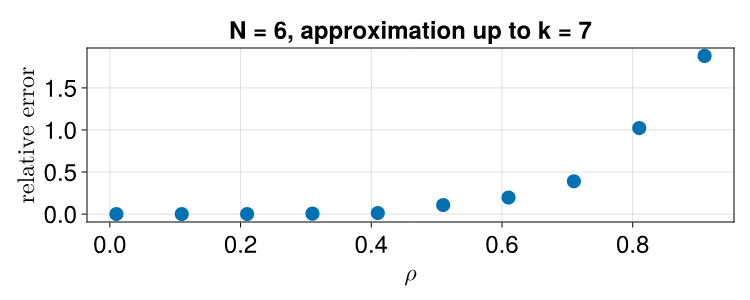
This expression renders explicit the link between the O-information and the motifs in the correlational matrix of a Gaussian system. Namely, even-length closed walks with and odd-length closed walks with contribute synergistically, while even-length closed walks with and odd-length closed walks with contribute redundantly. Therefore, Eq. (8) is minimized if is antibalanced, since for every closed walk in we have , ensuring the system to be synergy-dominated. In the Appendix A.3 Fig. 3 we show how this expansion approximates Eq. (2).
Our first result highlights the role of antibalanced correlational structures in synergistic Gaussian systems and provides a sufficient condition for synergy-dominance. We now explicitly consider what kind of patterns of interactions in linear processes can lead to synergistic correlational structures. Following a similar approach as in [31], we consider continuous Ornstein-Ulenbech (OU) processes which can be written as
| (9) |
where is the interaction matrix, is the identity matrix and is a Wiener process with covariance matrix equal to . If is symmetric and Schur stable, the covariance matrix of the resulting dynamics from Eq. (9) can be written as [31] (see also [32, 34]):
| (10) |
Then, the correlation matrix can be written as where if and otherwise. With this expression for in terms of the interaction matrix , we can use our previous results to show what interaction matrices lead to synergy-dominated systems.
Let us consider a system of size with no self-interactions, such that . Then, where and is the adjugate of , while . Thus, each element of can be written as
| (11) |
where for every pair and we have , and .
Now, consider the synergistic condition () for general correlation matrices of size . For simplicity, let . Then from Eq. (2) the system is synergy dominated if
| (12) |
where the RHS is always greater than zero since . In general, the antibalanced correlational structure is a sufficient condition for , as expected, and some solutions exist for (not shown). In what follows, we demonstrate that antibalanced interaction patterns are necessary for the system to be synergistic, covering the full spectrum of synergistic solutions.
To do this, we return to the interaction matrix and substitute the elements from Eq. (11), written in terms of , into the condition in Eq. (12). To simplify the following expressions we let . With some algebraic manipulations (see Appendix B.1), Eq. (12) can be shown to reduce to the form
| (13) |
where
Since the denominator in Eq. (13) is always positive and non-zero, and the term is squared, the synergistic condition reduces to , or equivalently
| (14) |
Note the RHS of Eq. (14) is always greater than zero since . Thus, for Eq. (14) to be satisfied we require , i.e., for the system to be synergistic we require the interaction matrix to be antibalanced.
We numerically confirm this result via a numerical parameter exploration of (Fig. 1). We compare the closed form solutions for , obtained by substituting Eq. (11) into Eq. (2), with the numerical O-information, denoted as , computed using the correlation matrix obtained from the simulated OU-process.

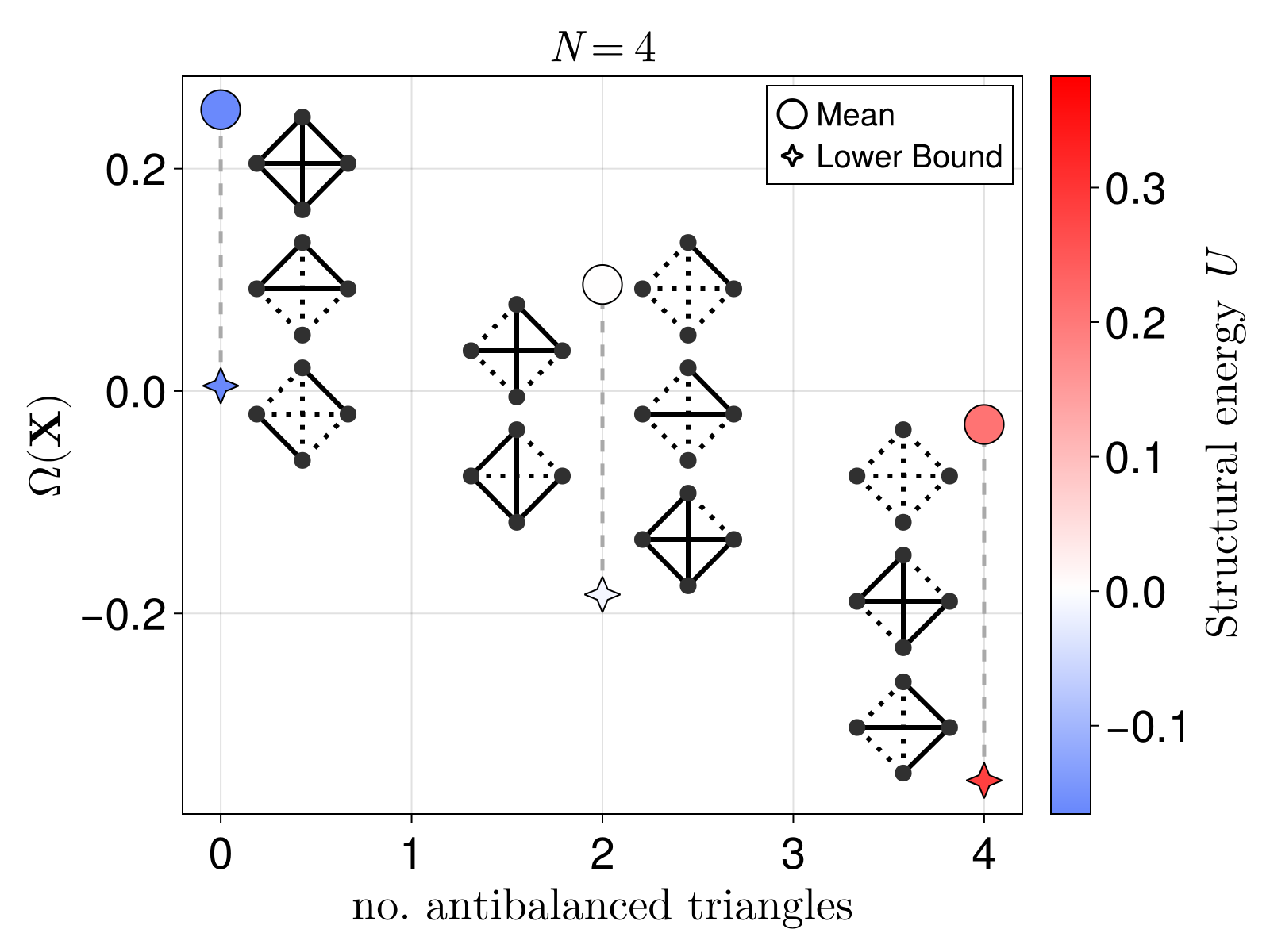
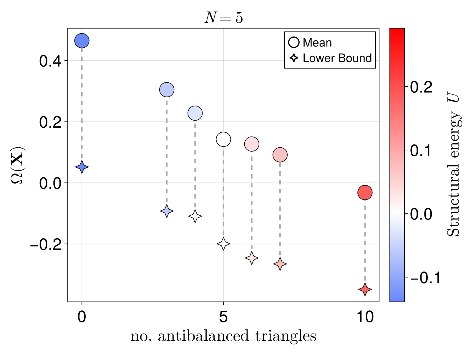
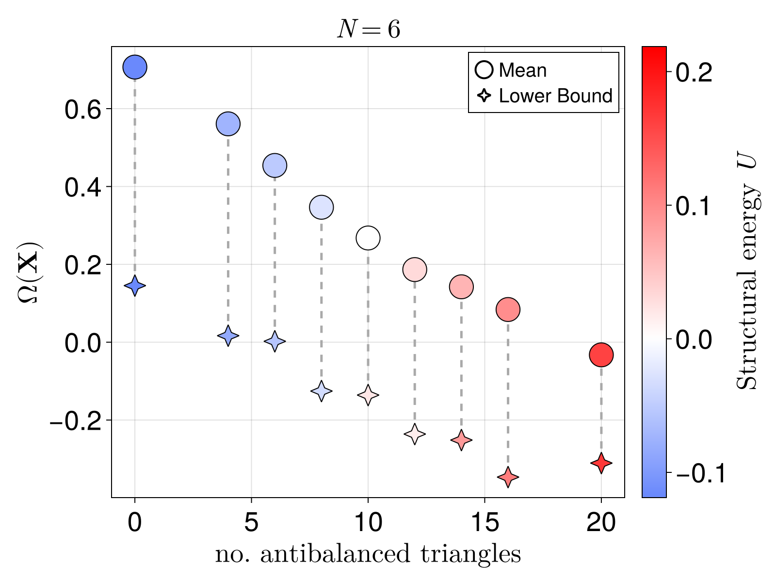
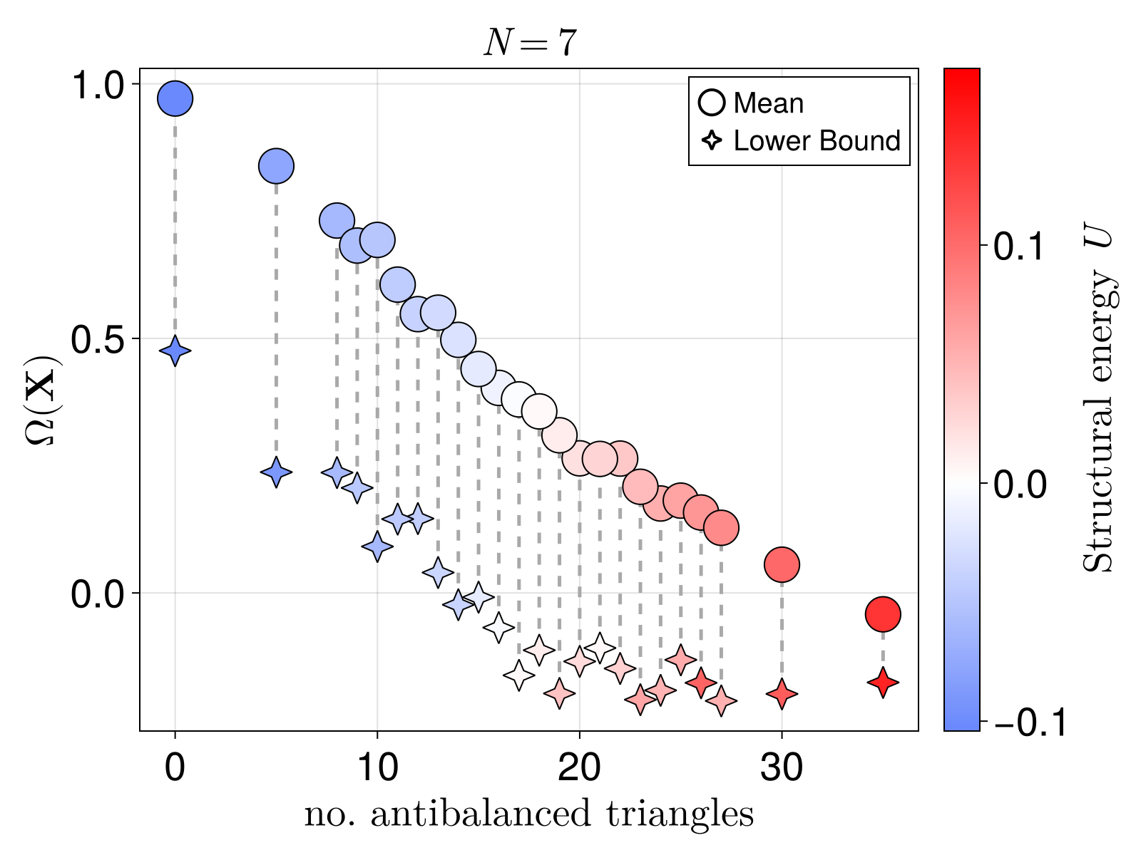
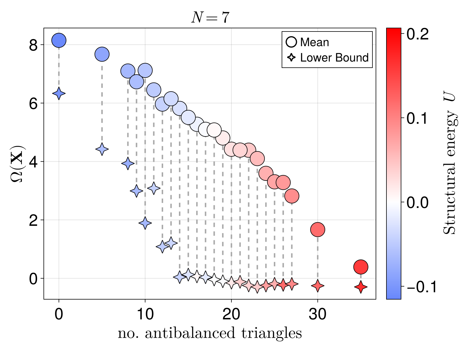
Next, we asked whether antibalanced interaction structures promote the emergence of synergistic information in larger dynamical systems. For systems of arbitrary dimension the elements of can be written in the same form as in Eq. (11). However, each is much more complex in higher-dimensions, as it consists of the minor of multiplied by its cofactor, making analytical insights much harder to obtain. Consequently, we performed extensive numerical explorations for systems of size . Since the O-information is order invariant, for each we studied all possible non-isomorphic complete signed graphs (graphs were constructed using the dataset in [35], see also Appendix B.2.1). This allowed us to systematically study all possible systems of size and determine the most synergistic interaction structures. We present our results in Fig. 2 for (see Appendix B.2.2 for other system’s sizes).

For any we studied, we found that the O-information is related to the number of antibalanced triangles or synergistic motifs in the interaction matrix . In particular, balanced interaction structures (with antibalanced triangles) always result in redundancy-dominated systems, while antibalanced structures (with antibalanced triangles) consistently result in systems with the lowest mean .
In summary, we proved that antibalanced pairwise interactions are necessary for synergy‐dominance in linear Gaussian systems without higher-order mechanisms, and that antibalanced correlational structures ensure synergy-dominance. In doing so, we reveal SBT as an instrumental conceptual lens for studying higher‐order interdependencies. Our analytically informed interpretation of the relation between SBT and IT is in line with observations of synergy in the classical Ising model and in coupled oscillatory systems, in the absence of higher-order mechanisms. In the Ising case, synergy peaks at the onset of the disorder-order phase transition [19]—driven by the emergence of conflicting spin alignments [20]. Similarly, competitive interactions in oscillatory systems were found to be crucial for the emergence of synergistic subsystems [21]. Taken together, our results demonstrate that purely pairwise interactions can give rise to higher-order behaviours and that these behaviours can be detected by simple correlational structures (motifs), thereby advancing our understanding of the relationship between mechanisms and behaviours in complex systems.
The expansion of the O-information (Eq. (8)) in terms of signed motifs of the correlation matrix shows that antibalanced correlational structures minimize . This result can be applied directly to empirical functional datasets where the Gaussian assumption holds—such as in whole-brain functional studies—to identify the most synergistic subsystems (but not all, see Eq. (12)), possibly improving current methods based on simulated annealing [28] or exhaustive [29] search.
Beyond applications, our theory could bridge the gap between approaches investigating higher-order phenomena and indicate novel research directions: () it clarifies how purely pairwise (low-order) mechanisms can give rise to higher-order interdependencies (synergy); () since the normalized leading term in Eq. (8) is equivalent to the SBT measure of a network’s structural energy [36]
| (15) |
our theory can explain why information-theoretic studies, such as [9, 28, 29], reach similar conclusions as in SBT-based neuroscience studies, such as [26]. Finally, it will be interesting to uncover the network-level dynamics—distinct from dynamics on networks with fixed topology—that lead to the formation of antibalanced interaction structures. In social balance theory, the formation of balanced triangles has largely been linked to higher-order mechanisms (e.g., triadic interactions), with only recent work showing that a simple pairwise homophily-based mechanism suffices [37]. Whether similar network mechanisms exist for the antibalanced case is an interesting and unexplored research question.
Acknowledgments
E.C. thanks Pedro A. M. Mediano for useful discussions, and for suggesting the study of OU processes.
References
- Jensen [2022] H. J. Jensen, Complexity science (Cambridge University Press, Cambridge, England, 2022).
- Williams and Beer [2010] P. L. Williams and R. D. Beer, Nonnegative decomposition of multivariate information (2010).
- Ince [2017] R. A. A. Ince, The partial entropy decomposition: Decomposing multivariate entropy and mutual information via pointwise common surprisal (2017).
- Gutknecht et al. [2021] A. J. Gutknecht, M. Wibral, and A. Makkeh, Bits and pieces: understanding information decomposition from part-whole relationships and formal logic, Proceedings of the Royal Society A: Mathematical, Physical and Engineering Sciences 477, 10.1098/rspa.2021.0110 (2021).
- van Enk [2023] S. J. van Enk, Quantum partial information decomposition, Physical Review A 108, 10.1103/physreva.108.062415 (2023).
- Javarone et al. [2024] M. A. Javarone, F. E. Rosas, P. Facchi, S. Pascazio, and S. Stramaglia, Quantifying high-order interdependencies in entangled quantum states, Physical Review A 109, 10.1103/physreva.109.042605 (2024).
- Rosas et al. [2019] F. E. Rosas, P. A. M. Mediano, M. Gastpar, and H. J. Jensen, Quantifying high-order interdependencies via multivariate extensions of the mutual information, Phys. Rev. E. 100, 032305 (2019).
- Sporns [2022] O. Sporns, The complex brain: connectivity, dynamics, information, Trends in Cognitive Sciences 26, 1066–1067 (2022).
- Luppi et al. [2022] A. I. Luppi, P. A. M. Mediano, F. E. Rosas, N. Holland, T. D. Fryer, J. T. O’Brien, J. B. Rowe, D. K. Menon, D. Bor, and E. A. Stamatakis, A synergistic core for human brain evolution and cognition, Nature Neuroscience 25, 771–782 (2022).
- Proca et al. [2024] A. M. Proca, F. E. Rosas, A. I. Luppi, D. Bor, M. Crosby, and P. A. M. Mediano, Synergistic information supports modality integration and flexible learning in neural networks solving multiple tasks, PLOS Computational Biology 20, e1012178 (2024).
- Tax et al. [2017] T. Tax, P. Mediano, and M. Shanahan, The partial information decomposition of generative neural network models, Entropy 19, 474 (2017).
- Rosas et al. [2022] F. E. Rosas, P. A. M. Mediano, A. I. Luppi, T. F. Varley, J. T. Lizier, S. Stramaglia, H. J. Jensen, and D. Marinazzo, Disentangling high-order mechanisms and high-order behaviours in complex systems, Nature Physics 18, 476–477 (2022).
- Neri et al. [2025] M. Neri, A. Brovelli, S. Castro, F. Fraisopi, M. Gatica, R. Herzog, P. A. M. Mediano, I. Mindlin, G. Petri, D. Bor, F. E. Rosas, A. Tramacere, and M. Estarellas, A taxonomy of neuroscientific strategies based on interaction orders, European Journal of Neuroscience 61, 10.1111/ejn.16676 (2025).
- Battiston et al. [2021] F. Battiston, E. Amico, A. Barrat, G. Bianconi, G. Ferraz de Arruda, B. Franceschiello, I. Iacopini, S. Kéfi, V. Latora, Y. Moreno, M. M. Murray, T. P. Peixoto, F. Vaccarino, and G. Petri, The physics of higher-order interactions in complex systems, Nature Physics 17, 1093–1098 (2021).
- Millán et al. [2025] A. P. Millán, H. Sun, L. Giambagli, R. Muolo, T. Carletti, J. J. Torres, F. Radicchi, J. Kurths, and G. Bianconi, Topology shapes dynamics of higher-order networks, Nature Physics 21, 353–361 (2025).
- Robiglio et al. [2025] T. Robiglio, M. Neri, D. Coppes, C. Agostinelli, F. Battiston, M. Lucas, and G. Petri, Synergistic signatures of group mechanisms in higher-order systems, Physical Review Letters 134, 10.1103/physrevlett.134.137401 (2025).
- Barrett [2015] A. B. Barrett, Exploration of synergistic and redundant information sharing in static and dynamical gaussian systems, Physical Review E 91, 10.1103/physreve.91.052802 (2015).
- Faes et al. [2017] L. Faes, D. Marinazzo, and S. Stramaglia, Multiscale information decomposition: Exact computation for multivariate gaussian processes, Entropy 19, 408 (2017).
- Marinazzo et al. [2019] D. Marinazzo, L. Angelini, M. Pellicoro, and S. Stramaglia, Synergy as a warning sign of transitions: The case of the two-dimensional ising model, Physical Review E 99, 10.1103/physreve.99.040101 (2019).
- Scagliarini et al. [2022] T. Scagliarini, D. Marinazzo, Y. Guo, S. Stramaglia, and F. E. Rosas, Quantifying high-order interdependencies on individual patterns via the local o-information: Theory and applications to music analysis, Physical Review Research 4, 10.1103/physrevresearch.4.013184 (2022).
- Luppi et al. [2024] A. I. Luppi, Y. Sanz Perl, J. Vohryzek, P. A. Mediano, F. E. Rosas, F. Milisav, L. E. Suarez, S. Gini, D. Gutierrez-Barragan, A. Gozzi, B. Misic, G. Deco, and M. L. Kringelbach, Competitive interactions shape brain dynamics and computation across species, bioRxiv 10.1101/2024.10.19.619194 (2024).
- Liardi et al. [2024] A. Liardi, F. E. Rosas, R. L. Carhart-Harris, G. Blackburne, D. Bor, and P. A. M. Mediano, Null models for comparing information decomposition across complex systems (2024).
- Harary [1953] F. Harary, On the notion of balance of a signed graph., Michigan Mathematical Journal 2, 10.1307/mmj/1028989917 (1953).
- Cartwright and Harary [1956] D. Cartwright and F. Harary, Structural balance: a generalization of heider’s theory., Psychological Review 63, 277–293 (1956).
- Healy and Stein [1973] B. Healy and A. Stein, The balance of power in international history: Theory and reality, Journal of Conflict Resolution 17, 33–61 (1973).
- Saberi et al. [2024] M. Saberi, J. R. Rieck, S. Golafshan, C. L. Grady, B. Misic, B. T. Dunkley, and A. Khatibi, The brain selectively allocates energy to functional brain networks under cognitive control, Scientific Reports 14, 10.1038/s41598-024-83696-7 (2024).
- Watanabe [1960] S. Watanabe, Information theoretical analysis of multivariate correlation, IBM Journal of Research and Development 4, 66–82 (1960).
- Varley et al. [2023a] T. F. Varley, M. Pope, J. Faskowitz, and O. Sporns, Multivariate information theory uncovers synergistic subsystems of the human cerebral cortex, Communications Biology 6, 10.1038/s42003-023-04843-w (2023a).
- Varley et al. [2023b] T. F. Varley, M. Pope, M. Grazia, Joshua, and O. Sporns, Partial entropy decomposition reveals higher-order information structures in human brain activity, Proceedings of the National Academy of Sciences 120, 10.1073/pnas.2300888120 (2023b).
- Cover and Thomas [2005] T. M. Cover and J. A. Thomas, Elements of Information Theory (Wiley, 2005).
- Barnett et al. [2009] L. Barnett, C. L. Buckley, and S. Bullock, Neural complexity and structural connectivity, Physical Review E 79, 10.1103/physreve.79.051914 (2009).
- Novelli et al. [2020] L. Novelli, F. M. Atay, J. Jost, and J. T. Lizier, Deriving pairwise transfer entropy from network structure and motifs, Proceedings of the Royal Society A: Mathematical, Physical and Engineering Sciences 476, 10.1098/rspa.2019.0779 (2020).
- Harary [2007] F. Harary, Structural duality, Behavioral Science 2, 255–265 (2007).
- Lizier et al. [2023] J. T. Lizier, F. Bauer, F. M. Atay, and J. Jost, Analytic relationship of relative synchronizability to network structure and motifs, Proceedings of the National Academy of Sciences 120, 10.1073/pnas.2303332120 (2023).
- [35] B. D. McKay, Dataset of simple graphs, https://users.cecs.anu.edu.au/~bdm/data/graphs.html, accessed: 27 May 2025.
- Marvel et al. [2009] S. A. Marvel, S. H. Strogatz, and J. M. Kleinberg, Energy landscape of social balance, Physical Review Letters 103, 10.1103/physrevlett.103.198701 (2009).
- Pham et al. [2022] T. M. Pham, J. Korbel, R. Hanel, and S. Thurner, Empirical social triad statistics can be explained with dyadic homophylic interactions, Proceedings of the National Academy of Sciences 119, 10.1073/pnas.2121103119 (2022).
Appendix A Static Systems
A.1 Gaussian O-information and derivations
Note that the of a Gaussian system with correlation matrix (with ones along the diagonal) can be written as
Then, from Eq. (1), we obtain
as reported in the main text.
A.2 Subsystem’s traces in terms of the whole trace
Recall that such that we can write the trace of a subsystem as
since is symmetric. Similarly,
So that when summing over we obtain and .
A.3 Walk expansion and link with SBT
Note that we can rewrite Eq. (7) from the main text as
| (16) |
since each closed walk has at least distinct vertices for even and at least distinct vertices for odd (recall also ). Then, from Eq. (5), we substitute in Eq. (16) to obtain
This expression can be more concisely written as
since and each walk has . Note, this expression is minimized if the correlational structure is antibalanced, since in this case is negative for odd-length closed walks and positive for even-length closed walks. In Fig. 3 we show how Eq. (8) approximates the O-information.
In general, it should be noted that, since each odd-length closed walk has at least distinct vertices, in Eq. (8) each of these walks is counted at least once. This is not the case for even-length closed walks since there exist many closed walks with only distinct vertices which disappear in Eq. (8). Then, it may be useful to rewrite Eq. (8) as
| (17) |
In this expression, the sign of the first summation term (order leading terms) is very similar to the structural energy metric used in [36, 26].
Appendix B Dynamical Systems
B.1 Synergy-dominance condition
After substituting the elements from Eq. (11) into the condition in Eq. (12) the LHS of Eq. (12) becomes
| (18) |
while the RHS
To simplify these, we multiply both sides by the common denominator which is always positive and non-zero. Taking the difference between the RHS and LHS we obtain
This expression can be written in the form
where
Since the first factor is always positive, we require to be positive for the condition to be satisfied, as shown in the main text.
B.2 OU process results
B.2.1 Methodology
To test how the O-information depends on the antibalanced structures in the interaction matrix of OU processes we studied the statistics of the resulting OU process dynamics using all possible sign configurations in the interaction matrix . More precisely, we computed from the covariance matrix of a OU process using all possible non-isomorphic complete signed graphs as interactions couplings. Note, there are many ways to sample . Here, we show additional results for interaction matrices with different average spectral radii and with or without self-interactions. Importantly, our results remain unaffected.
Note, here we studied all possible complete signed interactions networks (all-to-all couplings) since this can be done systematically. Studying all possible non-isomorphic signed graphs, including non-complete structures, is also possible. However, for non-complete graphs it is unclear how this can be done systematically, since there can be disconnected subgraphs and equivalent structures across scales. Additionally, the number of non-complete signed graphs increases with even faster than for the case for complete graphs.

Let be the set of adjacency matrices of all possible non-isomorphic unweighted complete signed graphs. For there are of these structures (Fig. 4), for there are , and for there are (see for instance the On-line Encyclopedia of large integer sequences, in what follows we used the dataset available here). Note, from the set of all non-isomorphic unsigned graphs we can obtain the set of all non-isomorphic complete signed graphs by replacing each missing edge with a negative edge (see Fig. 4). Each complete signed graph of size has triangles. In what follows, we use the variable to denote the number of antibalanced triangles. Importantly, two distinct structures and can have the same number of antibalanced triangles (for instance, see Fig. 5). For each of these structures we generated Schur stable matrices and computed the O-information of the theoretical expected covariance matrix of the resulting dynamics.
To generate a Schur stable matrices with desired sign patterns, we can sample a random symmetric matrix , multiply it element-wise with the adjacency matrix of the desired sign configuration, and then divide each element by the largest absolute eigenvalue to ensure stability, such that
| (19) |
where denotes element-wise multiplication between matrices. This method ensures that the largest absolute eigenvalue of the resulting interaction matrix will be less than (but very close to) unity, i.e., its spectral radius . To study interaction matrices with smaller spectral radii we can add a parameter , such that . For Fig. 2 in the main text we use to fix the spectral radius of the interaction matrices for to be . To see how the spectral radius affects the O-information, see Fig. 9 () and 9 () for the case for .
Using this procedure, we collected data for , which we show in Fig. (7, 7, 9 and 2). As noted earlier, two distinct signed graphs can have the same number of antibalanced triangles. This can be seen clearly for the case for (Fig. 5) where structures have , structures have and structures have . Let be the number of samples collected for each . The data here is the resulting from each sampled configuration matrix with antibalanced triangles. Then for the case for we have and . To avoid sample size effects we only used samples for each to compute the statistics we reported (similar for the cases with larger ).
B.2.2 Figures for