How Many Times Should We Matched Filter Gravitational Wave Data? A Comparison of GstLAL’s Online and Offline Performance
Abstract
Searches for gravitational waves from compact binary coalescences employ a process called matched filtering, in which gravitational wave strain data is cross-correlated against a bank of waveform templates. Data from every observing run of the LIGO, Virgo, and KAGRA collaboration is typically analyzed in this way twice, first in a low-latency mode in which gravitational wave candidates are identified in near-real time, and later in a high-latency mode. Such high-latency analyses have traditionally been considered more sensitive, since background data from the full observing run is available for assigning significance to all candidates, as well as more robust, since they do not need to worry about keeping up with live data. In this work, we present a novel technique to use the matched filtering data products from a low-latency analysis and re-process them by assigning significances in a high-latency way, effectively removing the need to perform matched filtering a second time. To demonstrate the efficacy of our method, we analyze 38 days of LIGO and Virgo data from the third observing run (O3) using the GstLAL pipeline, and show that our method is as sensitive and reliable as a traditional high-latency analysis. Since matched filtering represents the vast majority of computing time for a traditional analysis, our method greatly reduces the time and computational burden required to produce the same results as a traditional high-latency analysis. Consequently, it has already been adopted by GstLAL for the fourth observing run (O4) of the LIGO, Virgo, and KAGRA collaboration.
I Introduction
Ever since the first observing run (O1) of the LIGO Scientific Aasi et al. (2015), Virgo Acernese et al. (2015), and KAGRA Akutsu et al. (2020) collaboration, the field of gravitational-wave (GW) astronomy has proven to be an invaluable tool for probing the universe. By detecting mergers of black holes and neutron stars Abbott et al. (2019a); gwt (2021); The LIGO Scientific Collaboration et al. (2021); Abbott et al. (2021a), GW astronomy has given us the ability to study the universe in new ways. This has led to a host of new scientific results 245 and 247 (2017); Abbott et al. (2021b, 2020). GW searches are the first step to producing results within GW astronomy. These results are then used by downstream tools to facilitate multi-messenger astronomy, estimation of source parameters, and to perform studies on the population statistics and astrophysics of compact objects, cosmology, and tests of general relativity.
Only GWs produced by the mergers of the largest compact objects in the universe like black holes and neutron stars are loud enough to be observable by GW detectors like the Laser Interferometer Gravitational-wave Observatory (LIGO), Virgo, and KAGRA. Even then, GW signals reaching Earth are very faint, and heavily dominated by detector noise. Matched filtering Owen and Sathyaprakash (1999) is the primary tool employed by modeled GW searches to detect GW signals in noisy data. In this process, the data is cross-correlated against a template of a GW waveform predicted by general relativity, producing a signal-to-noise ratio (SNR) timeseries as output.
GstLAL Messick et al. (2017); Cannon et al. (2020); Sachdev et al. (2019); Hanna et al. (2020) is a stream-based GW search pipeline that has contributed to the LVK’s GW detections since O1. It implements time-domain matched filtering to recognize periods of time where GW signals are possibly buried in noise (called “triggers”). It then calculates a likelihood ratio (LR) Tsukada et al. (2023); Cannon et al. (2015, 2013) as a ranking statistic for assigning significance to these triggers. The triggers with particularly high LRs are retained and called GW candidates. Based on the LRs and rate of triggers recognized as noise, the LRs of candidates are converted to a false alarm rate (FAR), which represents our confidence in the candidate. Other search pipelines, such as PyCBC Canton et al. (2021); Davies et al. (2020); Nitz (2018), MBTA Aubin et al. (2021); Adams et al. (2016), SPIIR Chu (2022, 2017), and IAS Venumadhav et al. (2019); Zackay et al. (2021), also use similar techniques.
The GstLAL pipeline can operate in one of two modes: a low-latency “online” mode, or a high-latency “offline” mode. The online mode is designed to matched-filter the data, produce triggers, recognize candidates, and assign FARs in near-real time. The results are then immediately uploaded to the Gravitational Wave Candidate Event Database (GraceDB) Moe et al. (2014), from where a public alert can be sent if the upload meets certain criteria. The ability of GstLAL to produce results in near-real time and hence serve as an independent messenger in the detection of astronomical events is particularly useful. GW170817 LIGO Scientific Collaboration and Virgo Collaboration (2017); Abbott et al. (2017), a binary neutron star merger (BNS), is an excellent example of GW searches contributing to a multi-messenger detection, which led to many new scientific results Abbott et al. (2018, 2019b).
In contrast, the offline mode is designed to be run after all the data are available. The matched filtering, significance estimation, and FAR assignment stages are generally done one after the other in the offline analysis, and do not need to be done simultaneously like in the online analysis. Since the full background data can be used to assign significances to all candidates, it has traditionally been considered more sensitive than the online analysis. Since it operates in high latency, it is resilient to any processing delays, data availability delays, and hardware downtime. Consequently, it has also traditionally been considered more reliable and robust than the online analysis. Because of this, the process of matched filtering, which is otherwise identical for both operating modes, has always been repeated for the offline analysis by all search pipelines, after it was initially done in low-latency for the online analysis. Since GW searches are expensive, both in terms of time and computational resources, this repitition has a significant human and computational cost. With GW searches always looking to produce more scientific results, they are becoming ever larger, expanding to new parameter spaces, and analyzing more data than ever before. Consequently, the associated cost of running them is quickly starting to become unfeasible.
In this work, we address whether the repitition of matched filtering, which requires the overwhelming majority of computational power and time of any GW search, is necessary. In Sec. II, we describe the GstLAL pipeline and its two operating modes in detail. In Sec. III, we introduce a novel technique in which the data products created by the matched filtering of an online analysis are used in an offline fashion. In Sec. IV, we compare the results of this technique to a traditional offline analysis, to answer the question of whether data needs to matched-filtered a second time.
II Software
II.1 General GstLAL methods
The GstLAL workflow, in either operating mode, contains two broad stages: a setup stage, and a data processing stage. In the setup stage, input data products are precomputed for use during the data processing stage. Like all modeled GW searches, GstLAL uses a “bank” of GW waveform templates. The template bank ahead of O4 was generated using the manifold Hanna et al. (2023) software package as described in Sakon et al. (2022). It covers waveforms produced by binary mergers with component masses from 1-200 and dimensionless spins up to . This results in a bank containing approximately 2 million total waveforms.
The template bank is split into “template bins”, each of around 1000 templates, sorted by linear combinations of their Post-Newtonian phase coefficients Morisaki and Raymond (2020) as described in Sakon et al. (2022). The templates are additionally whitened using a power spectral density (PSD) that represents the frequency characteristics of detector noise in the data. The templates in a single template bin are processed together for the purpose of matched filtering and background collection, and consequently a single job within a GstLAL analysis corresponds to a specific template bin.
The next stage is the data processing stage. This involves the matched filtering process, significance assignment, FAR calculation, and uploading the results (the last only applicable for the online mode). The SNR timeseries produced by matched-filtering the data with a particular template is defined as:
| (1) |
where is the data whitened with the PSD, and is the similarly whitened template. Since matched filtering needs to be performed for the full data for every template, it is extremely computationally intensive. Though dependent on factors like cluster availability and computational power of the processors, we can calculate a rough estimate of the percent of time in an offline analysis taken up by matched filtering. The duration of the first half of O4 is around 8 months. An offline analysis over this period of time would take around 2 months. The setup stage, combined with significance assignment and FAR calculation takes around 1 day. That means matched filtering accounts for more than 98% of the time required for an offline analysis.
The SNR timeseries of every template is used to form triggers, by identifying times when the SNR exceeds the threshold value of 4. Parallelly, background data is also collected by identifying triggers that originate from noise Joshi et al. (2023). The background data thus collected is then used to rank the triggers using the likelihood ratio as described in Tsukada et al. (2023). Triggers with a high LR are retained as GW candidates, and the LRs of noise triggers, as well as the livetime of the analysis is used to convert the LRs of candidates into FARs.
In the following subsections, we will discuss how the implementation of these steps differs for the online and offline operating modes of the GstLAL analysis.
II.2 Online GstLAL Analysis
The online analysis is designed to ingest the data coming from the detectors in real-time, and produce results with minimal delay. While running an online analysis, if the FAR of a candidate crosses a certain threshold opa , it gets uploaded to GraceDB. Typically, this happens within 10-20 seconds of the GW reaching Earth Ewing et al. (2023). If certain other criteria are met, a skymap is generated showing the likely sky location of the source of the GW Singer and Price (2016); Singer et al. (2016); Ashton et al. (2019); Romero-Shaw et al. (2020), and a public alert is issued NASA . Additional information, such as low-latency parameter estimation of the source of the candidate Rose (2024), and the probability of astrophysical origin for different source classes Ray et al. (2023); Villa-Ortega et al. (2022); Andres et al. (2022) is also included in the public alert. Astronomers can then choose to follow up on this alert, and correlations can be made with other messengers Piotrzkowski (2022); Urban (2016); Cho (2019); Abbott et al. (2016). In this way, the online analysis plays an instrumental role in multi-messenger astronomy.
To facilitate this, the online analysis needs to ensure the following two principles are observed:
-
1.
Causality: To process a GW candidate, the analysis can only use data available up to that point in time. It cannot wait for more data to become available in the future.
-
2.
Keeping up with live data: The analysis cannot fall behind the incoming data. If it does, it needs to drop some data to catch up.
Currently, the GstLAL analysis has the ability to measure the PSD of the data in small batches of 4 seconds, and whiten the data accordingly, thus effectively ensuring causality well enough to serve the near-real time search. However, this ability does not extend to template whitening, and the templates need to be whitened during the setup stage. As a result, the online analysis uses a PSD projected to represent future noise, to whiten the templates. To minimize this effect, every week in O4, the GstLAL team has been whitening the templates used by the online analysis using the PSD measured over the previous week’s data. The expectation is that this captures any changes in the noise characteristics with a timescale equal to or larger than a week.
Additionally, to ensure causality, in order to rank a particular trigger, the online analysis can only use background data collected up to the point of that trigger. It cannot wait for the full background data to be collected. As a result, it may happen that the background used to rank a specific trigger has not converged fully, and so the LR and FAR assigned to that trigger are not as accurate as they would have been had we waited for the full background to be accumulated. Hence, the online analysis is traditionally considered to be less reliable.
Finally, to ensure the principle of keeping up with live data, if for any reason the analysis is unable to process some stretch of data, that data is permanetly lost. The analysis cannot go back and re-analyze the data. Data drops like this generally happen for one of three reasons:
-
1.
If the analysis hits a period of high latency, either due to its own internal processing, or due to external reasons like live data delivery failures, the analysis drops this data and moves on to newer data after waiting for a set amount of time (60 seconds).
-
2.
During the running of the analysis, there will be regularly scheduled maintenance, both internally for the analysis, and externally for the hardware it is running on. It is attempted to make these periods of downtime as short as possible, and to make them coincide with periods of time when the detectors are not producing data.
-
3.
Unintentional hardware downtime
Due to these reasons, the online analysis is traditionally considered to be less sensitive and robust as compared to an offline analysis.
II.3 Offline GstLAL Analysis
The offline analysis is designed to be robust, reliable, and more sensitive than the online analysis. It is typically used to generate more in-depth results than the online analysis, such as studies on population properties of compact binary systems Collaboration and the Virgo Collaboration (2021); Abbott et al. (2023), and tests of general relativity Abbott et al. (2019c, 2021c, 2016, b). To do this, offline analyses will commonly be run with simulated gravitational wave signals injected into the data. These are called “injections”, and they are used to measure the response of the analysis (i.e. the sensitivity) for GWs from sources in various parameter spaces, at different distances, etc.
The analysis is performed after the full data become available, and so there are no latency constraints. As a result, the analysis does not need to adhere to the principles of causality and keeping up with live data, like the online analysis did.
Consequently, the PSD used for template whitening can be directly measured from the full data itself, guaranteeing the best representaion of detector noise. In practice, the data are divided into week-long chunks, and the process of PSD measurement and template whitening is done separately for every chunk. This further improves how well we capture detector noise, and increases sensitivity.
Similarly, the filtering and ranking stages (which involves significance and FAR assignment), do not need to occur simultaneously for a given trigger in the offline analysis, and each stage can be done for all triggers before moving on to the next. This means that during the ranking stage, the background data from the full analysis can be used, leading to more reliable results, as well as an increase in sensitivity. With this in mind, the matched filtering stage and the ranking stage of the GstLAL offline workflow are completely modular, and designed to be run independently.
Additionally, the analysis does not need to drop data if it gets affected by some source of latency, whether it is a latency in its internal data processing or a disruption in data delivery. This means that the analysis is guaranteed to process all available data without dropping any like the online analysis, making it more reliable and sensitive. Furthermore, the analysis can make use of more robust data quality and data veto information, provided by external high-latency tools. This is thought to make the analysis more sensitive by removing obviously bad data that would have otherwise created false positives in both the candidates and the background.
III Methodology
In the descriptions of the online and offline GstLAL analyses above, the only differences between the matched filtering stages of the two are PSDs used for template whitening, and the fact that the two might not analyze exactly the same set of data. Since we expect the projected PSD used by the online analysis to still be a good approximation of the true PSD measured over the data that the offline analysis uses, the effect of PSD mismatch should be low Messick et al. (2017). Additionally, the weekly whitening of the online analysis templates using the previous week’s PSD will lower any SNR loss due to PSD mismatch further. Similarly, with improvements to the stability of the online analysis Ewing et al. (2023), data distribution, and computing hardware done before O4, we expect the effect of data drops to also be low. In Sec. IV we show that the online analysis only drops around 5% data as compared to the offline analysis, and also discuss ways to make up this lost 5%.
III.1 Online Rank
Based on this, we developed a novel technique that takes the data products created by the matched filter stage of an online analysis (i.e. triggers and background data), and replaces the offline analysis’ matched filter stage with these. The rest of the offline analysis (i.e. the ranking stage), is kept the same. This is possible since the two stages are designed to be modular, as described in Sec. II. We call this technique an “online rank”, since the matched filtering is taken from the online analysis, and an offline ranking stage is added to it.
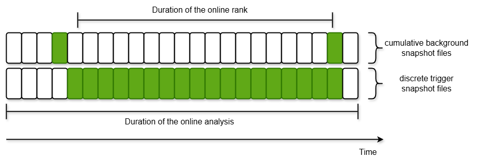
Alongside the modularity of the GstLAL offline workflow, the key to making an online rank possible is a feature of the GstLAL online analysis, called “snapshotting”. Every 4 hours, each job in the the online analysis (each corresponding to a template bin) will write a snapshot of the triggers and background data it has collected to disk. The trigger snapshot files are discrete, i.e. each file will only contain triggers created since the previous snapshot. In contrast, the background snapshot files are cumulative, i.e. each file will contain background data since the start of the analysis to the time of the snapshot. Snapshotting can also be used to save the progress of the online analysis in case something goes wrong and the analysis needs to be restored to a working state.
The setup process for an online rank involves going through all the trigger and background snapshot files written by the online analysis, and picking the relevant files to forward to the rank stage. The user can specify a start and end time for the online rank, which defines the duration of the online rank. Since trigger snapshot files are discrete, every trigger file whose duration (which is encoded in the filename) has an overlap with the duration of the online rank is forwarded to the rank stage. For the background snapshot files, however, since they are cumulative, the earliest snapshot file that contains all the background data of the duration of the online rank is chosen. If the start time of the online analysis is different from the start time of the online rank, the latest background snapshot file that doesn’t overlap at all with the duration of the online rank is also chosen. This is subtracted from the earlier file, to produce a background file that exactly contains the background data for the duration of the online rank, to the granularity of the 4 hour snapshots. This procedure is illustrated in Fig. 1. Typical of an offline analysis, this background file containing the full background data for the duration of the online rank is used to rank every trigger, leading to more reliable and sensitive results. Since trigger and background files are processed separately for every template bin, this process is repeated for every template bin. In this way, relevant files can be extracted from an online analysis that will typically be running for the full observing run, and offline results for a subset of the duration can be calculated from them. Since the snapshotting interval of 4 hours is relatively small as compared to typical analysis periods of many months, trigger and background data can be extracted from the online analysis for offline processing with high precision.
In order to make the online rank results even more reliable and sensitive, we can augment the inputs to the online rank with triggers and background data from times that the online analysis dropped. Specifically, for every job we calculate such a “dropped data segments”, which an offline filtering would have analyzed but the online filtering did not, and set up a traditional offline analysis using these dropped data segments. By combining the online rank inputs with the results of the dropped data refiltering analysis, we can be sure the online rank produces offline results for exactly the same periods of time that the traditional offline analysis would have. The typical amount of dropped data for any job is around 5% of the total time covered by the offline segments. This is demonstrated in Sec. IV. Additional details can also be found in Joshi et al. (2025).
III.2 Offline Rank Stage
After relevant trigger and background files for every template bin are chosen from the online analysis, they are forwarded to the offline rank stage. From this point on, the online rank analysis proceeds identically to the traditional offline analysis. Details of how the offline rank stage works can be found in Joshi et al. (2025).
III.3 Computational Cost Reduction
The online rank procedure requires an online analysis to have been run over the relevant period of data first. It enables us to re-use the matched filtering data products from the online analysis in order to get offline results. Since matched filtering is the bulk of the computational cost of any modeled GW search (98%, as discussed in Sec. II), over the course of an observing run (i.e. including running analyses to get both online and offline results), the online rank procedure represents approximately a 50% reduction in the total computational cose.
Given that the online analysis has alrady been run, we can calculate the time saved to get offline results via an online rank. Since the time required for matched filtering scales linearly with the amount of data analyzed, but the time required for an online rank does not strongly depend on the amount of data analyzed, the time saved because of the online rank method depends on the length of the analysis. The duration of the first half of O4 is around 8 months. The time required to perform a traditional offline analysis with injections over this period of time is approximately 4 months. We can get offline results for the same duration of time via an online rank in as low as 5 hours, if dropped data refiltering is not included. This represents a 99.8% reduction in the computational time in the best case scenario.
As discussed before, the typical amount of data dropped by an online analysis is 5%. This means that even if we choose to perform the dropped data refiltering analysis to augment the online rank, we still get approximately a 95% reduction in the amount of time required to get offline results.
IV Results
IV.1 MDC Data Set and Analyses
In order to test the efficacy of our new method, we ran an online analysis over a mock data challenge (MDC). This involved running the analysis over 38 days of O3 data from the LIGO Hanford and Livingston detectors, as well as the Virgo detector. The data extended from 7 January 15:59:42 UTC 2020 to 14 February 20:39:42 UTC 2020. These data were then shifted in time by 125952000 seconds to extend from 4 January 10:39:42 UTC 2024 to 11 February 15:19:42 UTC 2024, to make them appear as though they were live data when we ran the online analysis. The MDC also involved an injection campaign. More details about the MDC, including details about the injection set used can be found in Chaudhary et al. (2023).
We then performed an online rank on this analyis, as well as a traditional offline analysis on the same amount of data. After accounting for the times when no detectors were producing data, we find that the online rank had a livetime of 34.41 days, whereas the offline analysis had a livetime of 36.05 days. This means that over the course of 38 days, the online analysis dropped around 4.5% of the data. To compensate for this, we also performed a dropped data refiltering analysis over the 4.5% dropped data. All of these analyses were performed using the GstLAL O4 template bank, described in Sec. II.
IV.2 Sensitivity Comparisons
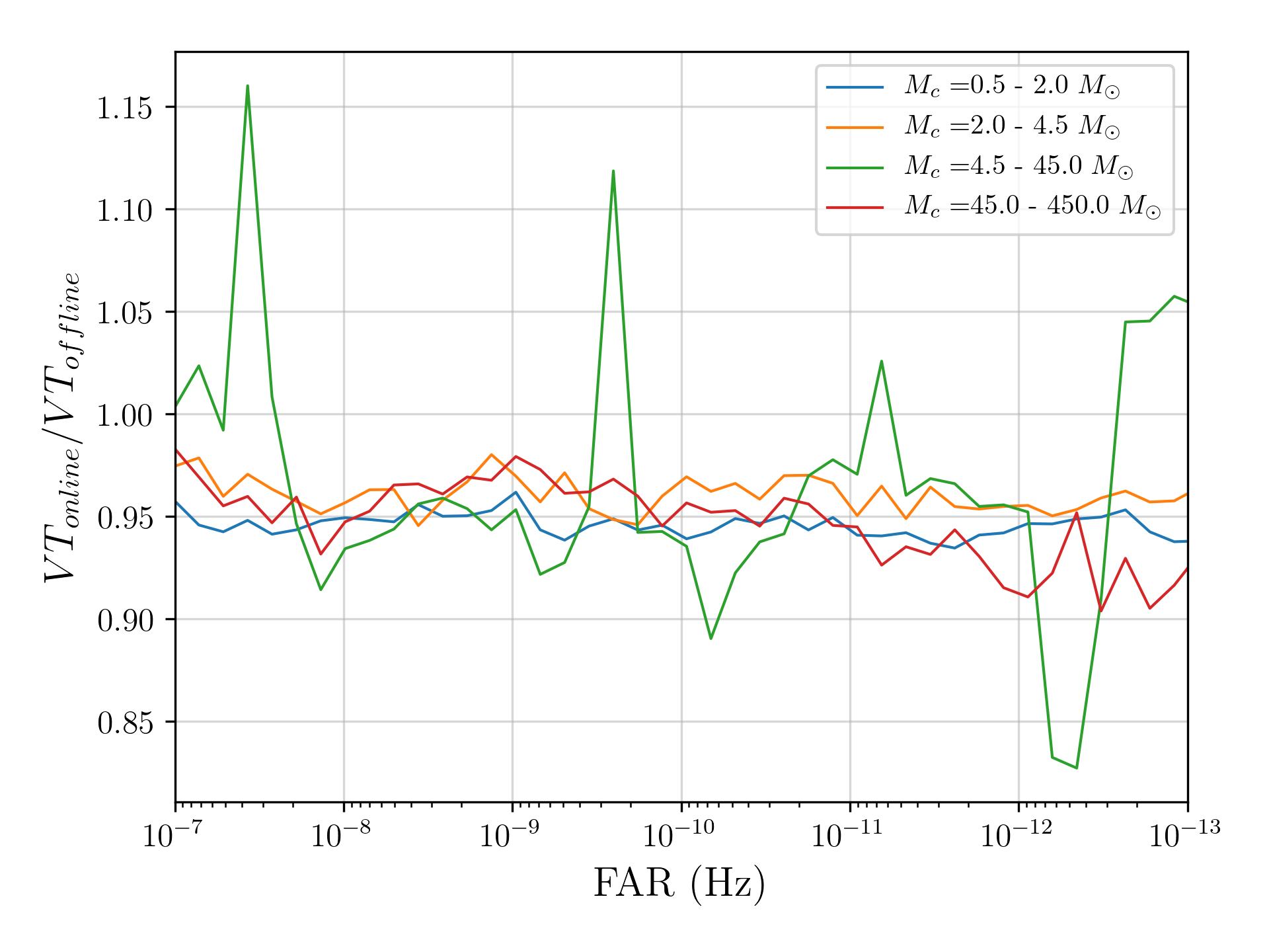
To compare the sensitivities of the online rank and the offline analysis, we can calculate the VTs of both, and then take the ratio of the two. Here, we have calculated the VT separately for injections with chirp mass in four different mass bins, roughly corresponding to four source categories: binary neutron star mergers (BNS, chirp mass between 0.5 to 2 ) neutron star-black hole mergers (NSBH, chirp mass between 2 to 4.5 ), binary black hole mergers (BBH, chirp mass between 4.5 to 45 ), and intermediate-mass black hole mergers (IMBH, chirp mass between 45 to 450 ). The VT is calculated at different FAR thresholds for considering an injection to be found by the analysis. The results of this VT comparison for different mass bins and FAR thresholds, for the pure online rank and offline analysis can be seen in Fig. 2. It shows us that the online rank is almost as sensitive as the offline analysis. We note that the 5% loss in the online rank VT as compared to the offline analysis lines up perfectly with the 5% of data dropped by the online analysis.
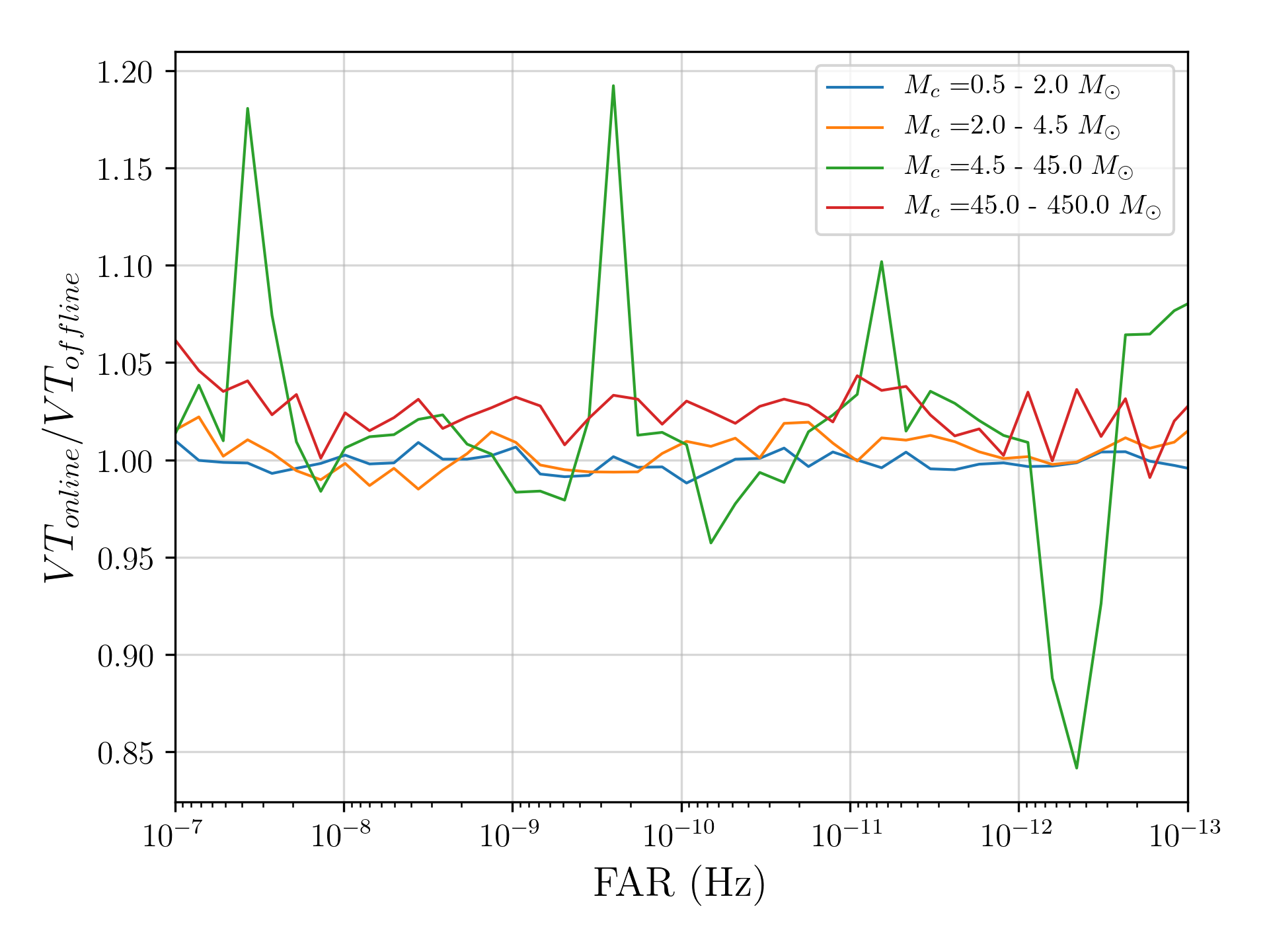
Next, we repeat the procedure for the online rank augmented with the dropped data refiltering analysis, and compare its VT to the VT of the offline analysis. The result of this is shown in Fig. 3. The fact that the VT ratios are now much closer to 1 tells us that the previous 5% loss in VT was indeed coming from dropped data, and that by augmenting an online rank with a dropped data refiltering analysis, we can get offline results that are as sensitive as a traditional offline analysis in a fraction of the time.
IV.3 Candidate Lists
Next, we compare the candidate lists from the online rank augmented with dropped data refiltering and offline analysis as a further check on the reliability and sensitivity of the online rank. There are 9 previously reported GW signals in the MDC data, and both analyses are able to detect 5 of them with a FAR of 1/month ( Hz) or less. The candidate list for the online rank is shown in Tab. 1, and that for the offline analysis is shown in Tab. 2. The top 10 candidates from both analyses are the same. Additionally, both analyses recover those 10 candidates with exactly the same template, as evidenced by the fact that they have the same primary and secondary masses ( and ), as well as the same dimensionless spins ( and ). Since the analyses were performed on O3 data shifted in time by 125952000 seconds, the reported times of the candidates do not match the times reported in the third Gravitational-Wave Transient Catalog Abbott et al. (2021a)
| Rank | FAR (Hz) | Time (UTC) | () | () | ||
|---|---|---|---|---|---|---|
| 1 | 2024-01-26 01:34:58 | 40.86 | 30.5 | 0.05 | 0.05 | |
| 2 | 2024-01-11 23:03:09 | 5.24 | 1.77 | -0.29 | -0.29 | |
| 3 | 2024-01-24 21:00:11 | 59.52 | 57.08 | 0.17 | 0.17 | |
| 4 | 2024-02-05 07:41:17 | 50.36 | 34.57 | -0.2 | -0.2 | |
| 5 | 2024-02-06 03:34:52 | 50.36 | 40.86 | -0.08 | -0.08 | |
| 6 | 2024-02-04 08:49:54 | 176.4 | 184.0 | 0.6 | 0.6 | |
| 7 | 2024-01-26 06:22:45 | 70.35 | 79.75 | 0.45 | 0.45 | |
| 8 | 2024-01-17 21:57:48 | 79.75 | 59.52 | -0.02 | -0.02 | |
| 9 | 2024-02-06 03:40:07 | 40.86 | 42.6 | 0.73 | 0.73 | |
| 10 | 2024-01-29 08:21:54 | 126.3 | 57.08 | -0.08 | -0.08 |
Out of the 9 previously reported GW candidates in this data, the ones not found significantly by either analyses are GW200208_222617, GW200112_155838, GW200202_154313, and GW200210_092254. The first of these was not found significantly by GstLAL even in Abbott et al. (2021a), and as such we do not expect it to be found significantly in either of the analyses performed here. The remaining three were recovered either as single detector candidates, or recovered confidently in only one detector. Because of the way GstLAL collects background data Joshi et al. (2023), these candidates were added to the background, and hence were downweighted, resulting in them not being recovered significantly. The method described in Joshi et al. (2023) is designed to prevent exactly this situation. However, it is currently only compatible with the online analysis (and hence the online rank), and in order to do a fair comparison, this method was not used for the analyses performed here. However, we did verify that by using this method in an online analysis, the online rank is able to recover all 3 of these candidates significantly. Since this method is used for O4, we expect GstLAL’s online ranks for O4 to be immune against such scenarios.
IV.4 Injection Parameter Recovery Comparisons
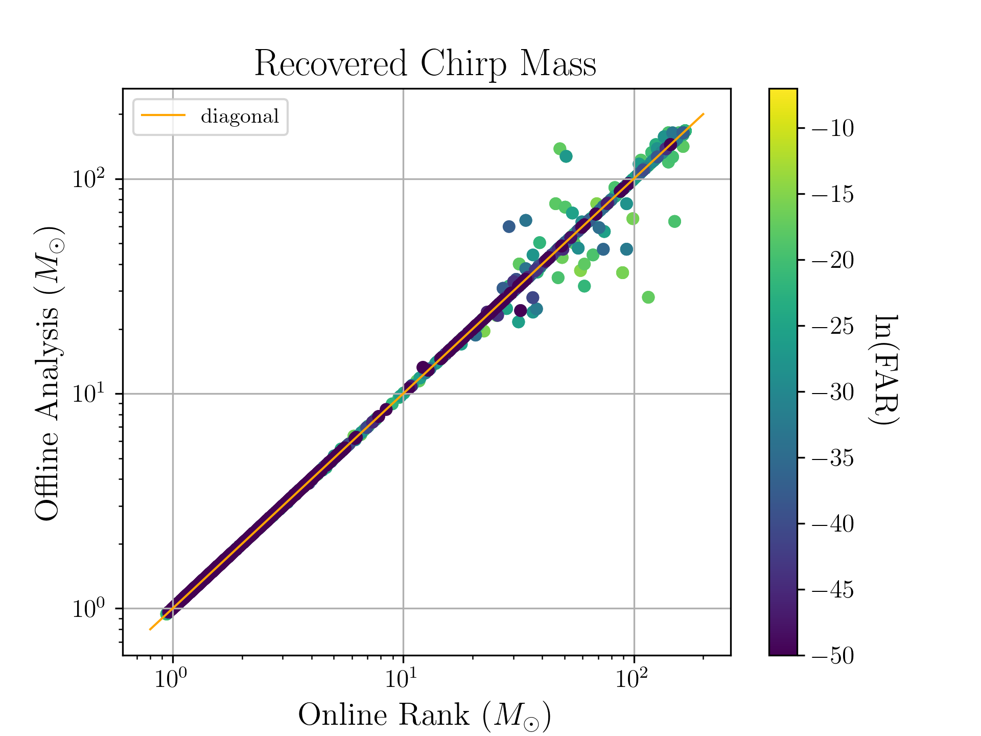
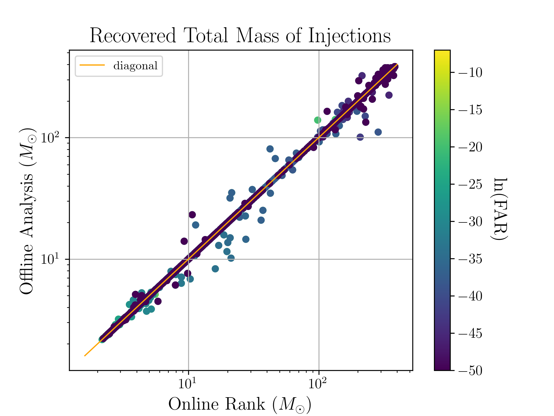
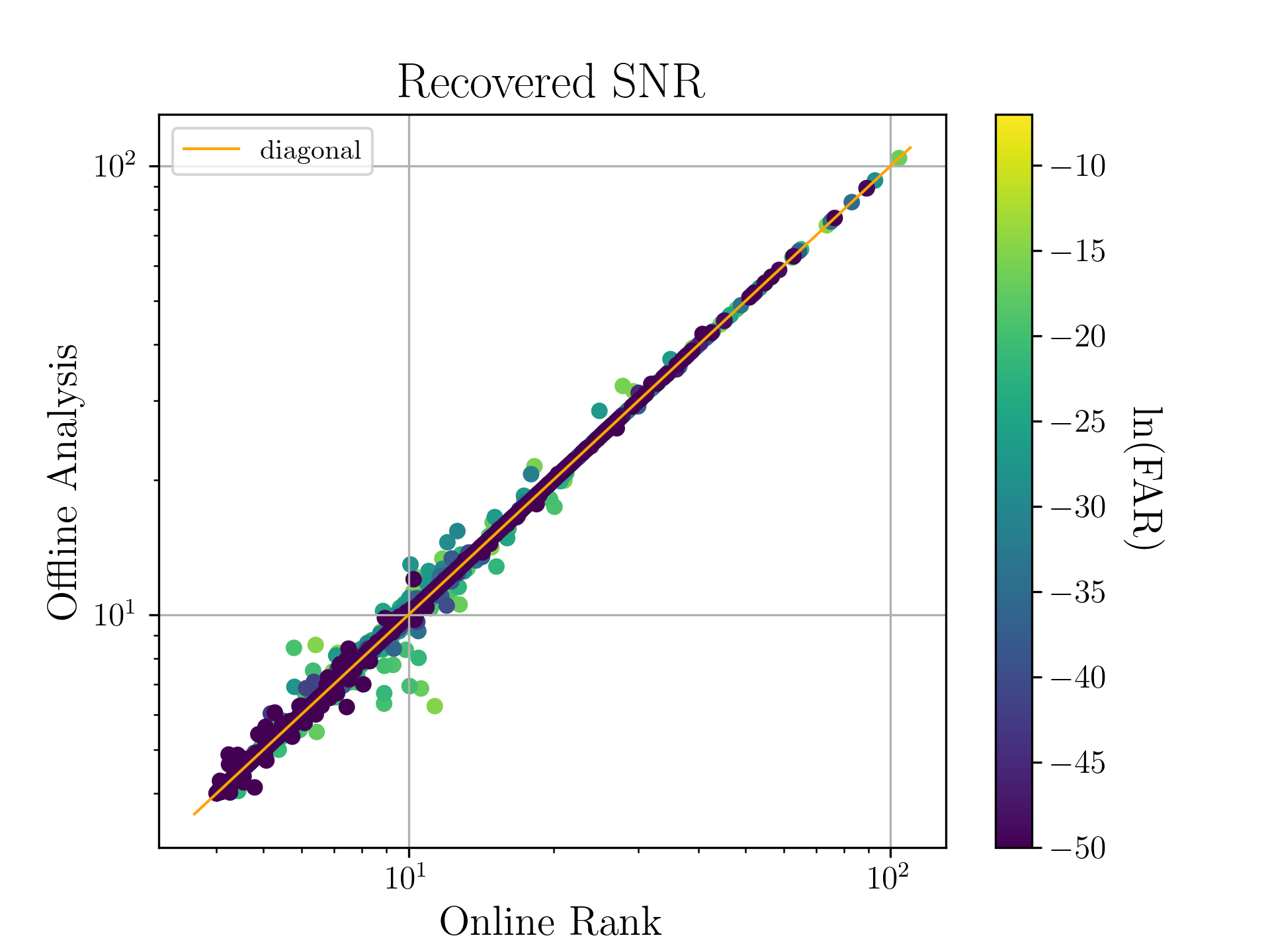
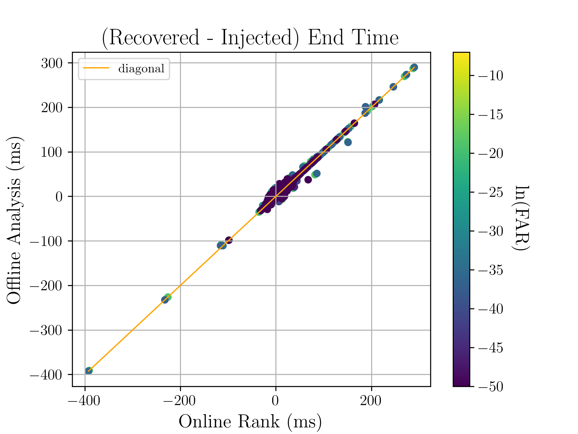
Since an injection campaign was conducted for both the online analysis (and hence the online rank), and the offline analysis, we can compare the parameters with which the online rank and offline analysis recovered injections. The FAR threshold used here for an injection to qualify as “found” is 1/month ( Hz). The parameters we compare here are the chirp mass, total mass, SNR, and coalescence time. Scatter plots of the values of these parameters recovered by the online rank and the offline analysis are shown in Fig. 4, Fig. 5, Fig. 6, and Fig. 7 respectively. In each figure, we see that almost all points are on the diagonal, with no systematic errors. This is further evidence that an online rank is very similar to a traditional offline analysis.
V Conclusion
In this work, we have decribed how a GstLAL analysis functions, and discussed the differences between the online and offline modes of operation. We introduced a new method called an online rank, in which the data products created by the matched filtering stage of an online analysis (i.e. triggers and background data), which are saved as 4 hour snapshots of the online analysis, can be taken and processed in an offline fashion. This removes the drawback that the online analysis has, of not having the full background information available while ranking triggers. Since matched filtering takes up the large majority of time required for an offline analysis, by not repeating the process of matched filtering, and taking the matched filtering results from the online analysis instead, we can get reliable and sensitive offline results in a fraction of the time compared to what is required for a traditional offline analysis. Over the course of an observing run (i.e. including both online and offline results), this represents a 50% reduction in total computational cost.
Furthermore, we discussed a technique called dropped data refiltering in which the matched filter outputs of the online analysis are augmented by a small offline analysis which analyzes times dropped by the online analysis. This ensures an online rank analyzes exactly the same period of time as an offline analysis.
To test our method, we performed an online analysis on 38 days of LIGO and VIRGO O3 data. We found that the online analysis had dropped around 5% data as compared to the offline analysis, consequently suffering a 5% loss in VT. By adding the dropped data refiltering outputs to the online rank, we were able to show the online rank is exactly as sensitive and reliable as a traditional offline analysis.
Due to the significant reductions in computational effort and time enabled by online rank method, we believe the future of GW searches lies in this paradigm, where in order to make detections in near-real time as well as produce more detailed results for the catalog, the data is matched filtered only once per observing run, by the online analysis. For O4, the GstLAL group has already adopted the online rank method, enabling fast and reliable offline results, as well as fast testing on new development work.
Acknowledgements.
This research has made use of data, software and/or web tools obtained from the Gravitational Wave Open Science Center (https://www.gw-openscience.org/ ), a service of Laser Interferometer Gravitational-Wave Observatory (LIGO) Laboratory, the LIGO Scientific Collaboration (LSC) and the Virgo Collaboration. We especially made heavy use of the LIGO Scientific, Virgo and KAGRA Collaboration (LVK) Algorithm Library. LIGO was constructed by the California Institute of Technology and the Massachusetts Institute of Technology with funding from the United States National Science Foundation (NSF) and operates under cooperative agreements PHYS- and PHY-. In addition, the Science and Technology Facilities Council (STFC) of the United Kingdom, the Max-Planck-Society (MPS), and the State of Niedersachsen/Germany supported the construction of Advanced Laser Interferometer Gravitational-Wave Observatory (aLIGO) and construction and operation of the GEO600 detector. Additional support for aLIGO was provided by the Australian Research Council. Virgo is funded, through the European Gravitational Observatory (EGO), by the French Centre National de Recherche Scientifique (CNRS), the Italian Istituto Nazionale di Fisica Nucleare (INFN) and the Dutch Nikhef, with contributions by institutions from Belgium, Germany, Greece, Hungary, Ireland, Japan, Monaco, Poland, Portugal, Spain. This material is based upon work supported by NSF’s LIGO Laboratory which is a major facility fully funded by the National Science Foundation. The authors are grateful for computational resources provided by the LIGO Lab culster at the LIGO Laboratory and supported by PHY- and PHY, the Pennsylvania State University’s Institute for Computational and Data Sciences gravitational-wave cluster, and supported by OAC-, PHY-, PHY-, OAC-, OAC-, and PHY-. LT acknowledges support from the Nevada Center for Astrophysics. CH Acknowledges generous support from the Eberly College of Science, the Department of Physics, the Institute for Gravitation and the Cosmos, the Institute for Computational and Data Sciences, and the Freed Early Career Professorship. M.W.C. acknowledges support from the National Science Foundation with grant numbers PHY-2308862 and PHY-2117997.References
- Aasi et al. (2015) J. Aasi et al. (LIGO Scientific), Class. Quant. Grav. 32, 074001 (2015), arXiv:1411.4547 [gr-qc] . equation of state (EoS)\xspace
- Acernese et al. (2015) F. Acernese et al. (VIRGO), Class. Quant. Grav. 32, 024001 (2015), arXiv:1408.3978 [gr-qc] .EoS\xspace
- Akutsu et al. (2020) T. Akutsu et al., Progress of Theoretical and Experimental Physics 2021 (2020), 10.1093/ptep/ptaa125, 05A101, https://academic.oup.com/ptep/article-pdf/2021/5/05A101/37974994/ptaa125.pdf .EoS\xspace
- Abbott et al. (2019a) B. P. Abbott et al. (LIGO Scientific, Virgo), Phys. Rev. X 9, 031040 (2019a), arXiv:1811.12907 [astro-ph.HE] .EoS\xspace
- gwt (2021) Physical Review X 11, 021053 (2021).EoS\xspace
- The LIGO Scientific Collaboration et al. (2021) The LIGO Scientific Collaboration, The Virgo Collaboration, R. Abbott, et al., “Gwtc-2.1: Deep extended catalog of compact binary coalescences observed by ligo and virgo during the first half of the third observing run,” (2021).EoS\xspace
- Abbott et al. (2021a) R. Abbott et al. (LIGO Scientific, VIRGO, KAGRA), “GWTC-3: Compact Binary Coalescences Observed by LIGO and Virgo During the Second Part of the Third Observing Run,” (2021a), arXiv:2111.03606 [gr-qc] .EoS\xspace
- 245 and 247 (2017) D. C. H. J. . K. V. . R. D. . T. L. . . S. D. . V. S. . Y. S. . . 245 and L. C. O. C. A. I. . . H. G. . . H. D. A. . . M. C. . . P. D. . V. S. . 247, Nature 551, 85 (2017).EoS\xspace
- Abbott et al. (2021b) R. Abbott, H. Abe, F. Acernese, K. Ackley, N. Adhikari, R. Adhikari, V. Adkins, V. Adya, C. Affeldt, D. Agarwal, et al., arXiv preprint arXiv:2112.06861 (2021b).EoS\xspace
- Abbott et al. (2020) R. Abbott, T. Abbott, S. Abraham, F. Acernese, K. Ackley, C. Adams, R. Adhikari, V. Adya, C. Affeldt, M. Agathos, et al., The Astrophysical Journal Letters 900, L13 (2020).EoS\xspace
- Owen and Sathyaprakash (1999) B. J. Owen and B. S. Sathyaprakash, Phys. Rev. D 60, 022002 (1999).EoS\xspace
- Messick et al. (2017) C. Messick et al., Phys. Rev. D 95, 042001 (2017), arXiv:1604.04324 [astro-ph.IM] .EoS\xspace
- Cannon et al. (2020) K. Cannon et al., “GstLAL: A software framework for gravitational wave discovery,” (2020), arXiv:2010.05082 [astro-ph.IM] .EoS\xspace
- Sachdev et al. (2019) S. Sachdev et al., “The GstLAL Search Analysis Methods for Compact Binary Mergers in Advanced LIGO’s Second and Advanced Virgo’s First Observing Runs,” (2019), arXiv:1901.08580 [gr-qc] .EoS\xspace
- Hanna et al. (2020) C. Hanna et al., Phys. Rev. D101, 022003 (2020), arXiv:1901.02227 [gr-qc] .EoS\xspace
- Tsukada et al. (2023) L. Tsukada, P. Joshi, S. Adhicary, R. George, A. Guimaraes, C. Hanna, R. Magee, A. Zimmerman, P. Baral, A. Baylor, K. Cannon, S. Caudill, B. Cousins, J. D. E. Creighton, B. Ewing, H. Fong, P. Godwin, R. Harada, Y.-J. Huang, R. Huxford, J. Kennington, S. Kuwahara, A. K. Y. Li, D. Meacher, C. Messick, S. Morisaki, D. Mukherjee, W. Niu, A. Pace, C. Posnansky, A. Ray, S. Sachdev, S. Sakon, D. Singh, R. Tapia, T. Tsutsui, K. Ueno, A. Viets, L. Wade, and M. Wade, (2023), arXiv:2305.06286 [astro-ph.IM] .EoS\xspace
- Cannon et al. (2015) K. Cannon, C. Hanna, and J. Peoples, “Likelihood-Ratio Ranking Statistic for Compact Binary Coalescence Candidates with Rate Estimation,” (2015), arXiv:1504.04632 [astro-ph.IM] .EoS\xspace
- Cannon et al. (2013) K. Cannon, C. Hanna, and D. Keppel, Phys. Rev. D 88, 024025 (2013), arXiv:1209.0718 [gr-qc] .EoS\xspace
- Canton et al. (2021) T. D. Canton, A. H. Nitz, B. Gadre, G. S. C. Davies, V. Villa-Ortega, T. Dent, I. Harry, and L. Xiao, The Astrophysical Journal 923, 254 (2021).EoS\xspace
- Davies et al. (2020) G. S. Davies, T. Dent, M. Tápai, I. Harry, C. McIsaac, and A. H. Nitz, Physical Review D 102 (2020), 10.1103/physrevd.102.022004.EoS\xspace
- Nitz (2018) A. H. Nitz, Physical Review D 98 (2018), 10.1103/PhysRevD.98.024050.EoS\xspace
- Aubin et al. (2021) F. Aubin, F. Brighenti, R. Chierici, D. Estevez, G. Greco, G. M. Guidi, V. Juste, F. Marion, B. Mours, E. Nitoglia, O. Sauter, and V. Sordini, Classical and Quantum Gravity 38, 095004 (2021).EoS\xspace
- Adams et al. (2016) T. Adams, D. Buskulic, V. Germain, G. M. Guidi, F. Marion, M. Montani, B. Mours, F. Piergiovanni, and G. Wang, Classical and Quantum Gravity 33, 175012 (2016).EoS\xspace
- Chu (2022) Q. Chu, Physical Review D 105 (2022), 10.1103/PhysRevD.105.024023.EoS\xspace
- Chu (2017) Q. Chu, Low-latency detection and localization of gravitational waves from compact binary coalescences, Ph.D. thesis, The University of Western Australia (2017).EoS\xspace
- Venumadhav et al. (2019) T. Venumadhav, B. Zackay, J. Roulet, L. Dai, and M. Zaldarriaga, Phys. Rev. D 100, 023011 (2019).EoS\xspace
- Zackay et al. (2021) B. Zackay, L. Dai, T. Venumadhav, J. Roulet, and M. Zaldarriaga, Physical Review D 104 (2021), 10.1103/physrevd.104.063030.EoS\xspace
- Moe et al. (2014) B. Moe, P. Brady, B. Stephens, E. Katsavounidis, R. Williams, and F. Zhang, “GraceDB: A Gravitational Wave Candidate Event Database,” (2014).EoS\xspace
- LIGO Scientific Collaboration and Virgo Collaboration (2017) LIGO Scientific Collaboration and Virgo Collaboration, GCN 21505 (2017).EoS\xspace
- Abbott et al. (2017) B. P. Abbott et al. (LIGO Scientific, Virgo), Phys. Rev. Lett. 119, 161101 (2017), arXiv:1710.05832 [gr-qc] .EoS\xspace
- Abbott et al. (2018) B. P. Abbott et al. (The LIGO Scientific Collaboration and the Virgo Collaboration), Phys. Rev. Lett. 121, 161101 (2018).EoS\xspace
- Abbott et al. (2019b) B. P. Abbott et al. (LIGO Scientific Collaboration and Virgo Collaboration), Phys. Rev. Lett. 123, 011102 (2019b).EoS\xspace
- Hanna et al. (2023) C. Hanna, J. Kennington, S. Sakon, S. Privitera, M. Fernandez, J. Wang, C. Messick, A. Pace, K. Cannon, P. Joshi, R. Huxford, S. Caudill, C. Chan, B. Cousins, J. D. E. Creighton, B. Ewing, H. Fong, P. Godwin, R. Magee, D. Meacher, S. Morisaki, D. Mukherjee, H. Ohta, S. Sachdev, D. Singh, R. Tapia, L. Tsukada, D. Tsuna, T. Tsutsui, K. Ueno, A. Viets, L. Wade, and M. Wade, Phys. Rev. D 108, 042003 (2023).EoS\xspace
- Sakon et al. (2022) S. Sakon et al., “Template bank for compact binary mergers in the fourth observing run of Advanced LIGO, Advanced Virgo, and KAGRA,” (2022), arXiv:2211.16674 [gr-qc] .EoS\xspace
- Morisaki and Raymond (2020) S. Morisaki and V. Raymond, Phys. Rev. D 102, 104020 (2020), arXiv:2007.09108 [gr-qc] .EoS\xspace
- Joshi et al. (2023) P. Joshi, L. Tsukada, and C. Hanna, “Background Filter: A method for removing signal contamination during significance estimation of a GstLAL anaysis,” (2023), arXiv:2305.18233 [gr-qc] .EoS\xspace
- (37) “Igwn public alerts user guide,” https://emfollow.docs.ligo.org/userguide/analysis/index.html##alert-threshold.EoS\xspace
- Ewing et al. (2023) B. Ewing, R. Huxford, D. Singh, L. Tsukada, C. Hanna, Y.-J. Huang, P. Joshi, A. K. Y. Li, R. Magee, C. Messick, A. Pace, A. Ray, S. Sachdev, S. Sakon, R. Tapia, S. Adhicary, P. Baral, A. Baylor, K. Cannon, S. Caudill, S. S. Chaudhary, M. W. Coughlin, B. Cousins, J. D. E. Creighton, R. Essick, H. Fong, R. N. George, P. Godwin, R. Harada, J. Kennington, S. Kuwahara, D. Meacher, S. Morisaki, D. Mukherjee, W. Niu, C. Posnansky, A. Toivonen, T. Tsutsui, K. Ueno, A. Viets, L. Wade, M. Wade, and G. Waratkar, (2023), arXiv:2305.05625 [gr-qc] .EoS\xspace
- Singer and Price (2016) L. P. Singer and L. R. Price, “Rapid Bayesian position reconstruction for gravitational-wave transients,” (2016), arXiv:1508.03634 [gr-qc] .EoS\xspace
- Singer et al. (2016) L. P. Singer et al., Astrophys. J. Lett. 829, L15 (2016), arXiv:1603.07333 [astro-ph.HE] .EoS\xspace
- Ashton et al. (2019) G. Ashton et al., Astrophys. J. Suppl. 241, 27 (2019), arXiv:1811.02042 [astro-ph.IM] .EoS\xspace
- Romero-Shaw et al. (2020) I. M. Romero-Shaw et al., Mon. Not. Roy. Astron. Soc. 499, 3295 (2020), arXiv:2006.00714 [astro-ph.IM] .EoS\xspace
- (43) NASA, GCN .EoS\xspace
- Rose (2024) C. A. Rose, Rapid Parameter Estimation of Compact Binary Coalescences with Gravitational Waves, Ph.D. thesis, The University of Wisconsin-Milwaukee (2024).EoS\xspace
- Ray et al. (2023) A. Ray et al., “When to Point Your Telescopes: Gravitational Wave Trigger Classification for Real-Time Multi-Messenger Followup Observations,” (2023), arXiv:2306.07190 [gr-qc] .EoS\xspace
- Villa-Ortega et al. (2022) V. Villa-Ortega, T. Dent, and A. C. Barroso, arXiv preprint arXiv:2203.10080 (2022).EoS\xspace
- Andres et al. (2022) N. Andres, M. Assiduo, F. Aubin, R. Chierici, D. Estevez, F. Faedi, G. M. Guidi, V. Juste, F. Marion, B. Mours, E. Nitoglia, and V. Sordini, Classical and Quantum Gravity 39, 055002 (2022).EoS\xspace
- Piotrzkowski (2022) B. Piotrzkowski, Searching for Gravitational Wave Associations with High-Energy Astrophysical Transients, Ph.D. thesis, The University of Wisconsin-Milwaukee (2022).EoS\xspace
- Urban (2016) A. L. Urban, Monsters in the dark: High energy signatures of black hole formation with multimessenger astronomy, Ph.D. thesis, The University of Wisconsin-Milwaukee (2016).EoS\xspace
- Cho (2019) M.-A. Cho, Low-latency searches for gravitational waves and their electromagnetic counterparts with Advanced LIGO and Virgo, Ph.D. thesis, University of Maryland, College Park (2019).EoS\xspace
- Abbott et al. (2016) B. P. Abbott et al., apjl 826, L13 (2016), arXiv:1602.08492 [astro-ph.HE] .EoS\xspace
- Collaboration and the Virgo Collaboration (2021) T. L. S. Collaboration and the Virgo Collaboration, The Astrophysical Journal Letters 913, L7 (2021).EoS\xspace
- Abbott et al. (2023) R. Abbott et al. (KAGRA, VIRGO, LIGO Scientific), Phys. Rev. X 13, 011048 (2023), arXiv:2111.03634 [astro-ph.HE] .EoS\xspace
- Abbott et al. (2019c) B. P. Abbott et al. (The LIGO Scientific Collaboration and the Virgo Collaboration), Phys. Rev. D 100, 104036 (2019c).EoS\xspace
- Abbott et al. (2021c) R. Abbott et al. (LIGO Scientific Collaboration and Virgo Collaboration), Phys. Rev. D 103, 122002 (2021c).EoS\xspace
- Abbott et al. (2016) B. P. Abbott et al. (LIGO Scientific and Virgo Collaborations), Phys. Rev. Lett. 116, 221101 (2016).EoS\xspace
- Joshi et al. (2025) P. Joshi et al., “New methods for offline gstlal analyses,” In preparation (2025).EoS\xspace
- Chaudhary et al. (2023) S. S. Chaudhary et al., “Low-latency alert products and their performance in anticipation of the fourth ligo-virgo-kagra observing run,” (in prep) (2023).EoS\xspace