Critical Dynamics of Random Surfaces
and Multifractal Scaling
Abstract
The critical dynamics of conformal field theories on random surfaces is investigated beyond the dynamics of the overall area and the genus. It is found that the evolution of the order parameter in physical time is a multifractal random walk. Accordingly, the higher moments of time variations of the order parameter exhibit multifractal scaling. The series of Hurst exponents is computed and illustrated with the examples of the Ising-, 3-state-Potts-, and general minimal models on a random surface. Models are identified that can replicate the observed multifractal scaling in financial markets.
1 Introduction
Conformal field theories with central charge on random surfaces have been proposed as toy models of string theory in two or fewer embedding dimensions.
Their field theory has been developed in [1, 2, 3, 4].
Recently, it has been argued [5] that these models may also have another application outside of string theory, namely as
the continuum limits of certain social networks that are self-driven to a critical point, such as financial markets [6].
Motivated by this conjecture, we have begun to develop the critical dynamics [7] of these models (see [8, 9] for a review of critical dynamics).
In [5], the focus was on an extended minisuperspace approximation, where only the overall area and the genus of the random surface are dynamical
variables. Regarding the dynamics of the area, we have found that the area evolves in physical time according to a Cox-Ingersol-Ross process.
Genus-zero surfaces shrink; to prevent them from shrinking to zero, a small-area cutoff is needed. Higher-genus surfaces grow
until their area is of the order of the inverse cosmological constant.
Regarding the dynamics of the genus, we have concluded from the matrix model results [10, 11, 12] that it leads to two distinct phases:
-
•
A planar phase, in which the ensemble of random surfaces is dominated by surfaces of genus zero or low genus. In this phase, we expect nontrivial critical phenomena.
-
•
A foamy phase, in which handles condense and all nodes are highly connected. This phase is presumably described by mean field theory, yielding a simple scaling behavior.
In this paper, we investigate the planar phase in more detail. We extend the previous study [5] to the dynamics of the order parameter
of a field theory that lives on the random surface,
such as the overall magnetization in the case of the Ising model.
This involves computing correlation functions of the so-called “gravitational dressing” of the order parameter, which
makes it necessary to go beyond the minisuperspace approximation.
Our main result is that the order parameter performs a multifractal random walk, as introduced in [13].
Correspondingly, the higher moments of time variations of the order parameter display multifractal scaling [14].
We approximately compute all Hurst exponents. In first approximation, the Ising model, the 3-state Potts model, and other minimal models
including non-unitary ones can replicate the multifractal scaling that has been empirically
observed in financial markets (see [15] for early observations and [16, 17] for reviews).
This paper is organized as follows. Sections 2, 3, and 4 briefly review the usual mono-scaling of critical dynamics on a flat surface, the multifractal random walk, and random surfaces in conformal gauge, respectively. Section 5 derives the multifractal walk in background time on a random surface of fixed total area. Section 6 translates it into a multifractal random walk in physical time. Section 7 approximately computes the corresponding Hurst exponents. Section 8 illustrates the results with examples of the minimal models on a random surface, and compares with empirical observations for financial markets.
2 Mono-Scaling on a Static Surface
We first consider a conformal field theory (CFT), such as the Ising model at its critical point, on a static (as opposed to random) surface of area . We assume that it evolves in time according to “model A” of critical dynamics [7] (see also [5]). Let be a matter primary field of dimension , such as the spin field with dimension in the case of the Ising model. As an an order parameter, we use the integral of over at time :
| (1) |
The main subject of this paper are the moments of the distribution of what we call the “returns” of the order parameter, i.e., its time variations over a given time horizon :
| (2) |
On a static surface of area , the second moment (the variance of returns) scales as [6]
| (3) |
where is the so-called dynamic critical exponent which defines extended 2+1-dimensional scale transformations . Classically, . At 1-loop level, , where . The prefactor in (3) reflects translation invariance on the surface . (3) follows from the renormalization group by requiring the correct behavior under scale transformations in background space and time,
as well as consistency with the limit of an ordinary random walk with linearly growing variance . In (3), we have included an arbitrary function of the scale-invariant combination , which is allowed by the renormalization group but must drop out in the infinite area limit. For higher moments, scaling implies:
| (4) |
For even , the Hurst exponents are defined as follows:
| (5) |
For a CFT in flat space, we see that all Hurst exponents are equal, which is called “mono-scaling”. If the Hurst exponents depend on , one speaks of “multifractal scaling” or “multi-scaling” [14]. In the following, we will show that multifractal scaling occurs if the CFT lives on a random surface.
3 Multifractal Random Walk (MRW)
Specifically, we will show that the order parameter performs a variant of the “multifractal random walk”, which was introduced in [13]
and aspects of which we first briefly review.
Viewed as a stochastic process, in (1) may be a Gaussian random walk with , or a fractional random walk with . The authors of [13] consider the situation where is coupled to a Gaussian random variable with variance and logarithmic auto-correlation in time:
| (6) |
The divergences at are rgularized by a short-time cutoff and a correlation time . is a free real parameter of the model, and is interpreted as “stochastic volatility” in the sense that it multiplies the time variations of :
This modifies their moments (2) to
| (7) |
Compared with the authors of [13], who work with the bare field ,
we will work with the renormalized field .
This removes the divergent expectation value of of [13], while acquires an anomalous dimension .
The following is shown in [13]: in the simpler case of a Gaussian random walk, . Integrating out in (7) thus pairs the operators into . For even , there are links between such pairs, which yields the scaling
This yields the Hurst exponents
If is a fractional random walk with , one instead obtains the Hurst exponents [13]
| (8) |
They thus display multifractal scaling with the time interval , decreasing linearly with . This implies that the shape of the return distribution is not scale invariant. In particular, its tails are ”fatter” for shorter time horizons. E.g., the kurtosis decreases with until it reaches some value (the Gaussian value) at the correlation time.
4 Random Surfaces in Conformal Gauge
To explain why such a multifractal random walk arises
when a conformal field theory (CFT), called the “matter”, with central charge (such as the Ising model with ) is put on a random surface,
we first recall a few aspects of the theory of random surfaces.
Let our 2-dimensional CFT contain primary fields with of scaling dimensions , and let it live on a random surface of genus . In conformal gauge, we can locally write the two-dimensional metric as , where is an arbitrarily chosen background metric with curvature , and is the logarithm of the conformal factor. Recall that the following effective action for arises from the conformal anomaly [1, 2, 3, 4]:
| (9) |
where and are renormalization parameters, is the renormalized area, is the two-dimensional cosmological constant, is a small coupling constant, and is the so-called “gravitational dressing” of . This theory must be independent of the fictitious background metric , and, in particular, scale invariant. Therefore the central charge of the combined matter--theory must be zero, and the operators must have dimension 2 before integration over the surface. This can been seen to imply [3, 4]:
| (10) |
E.g., for the Ising model, one obtains .
What is the dimension of the field after it has been put on the random surface? This question seems puzzling at first: as the theory is scale invariant, the coupling constant does not “run” at all under background scale transformations. Then how can there be a nontrivial dimension? The answer is, we must examine the behavior of under physical scale transformations. Since the area has dimension , physical (as opposed to background) rescalings by a factor correspond to constant shifts of the field :
| (11) |
Thus, the physical scale dependence is encoded in the
-dependence of . Therefore, the “gravitationally dressed” dimension of is
before integrating over the two-dimensional surface. E.g., for the Ising model, .
As described in [5], to study the critical dynamics of the CFT on a random surface, we introduce a background time , which trivially extends the two-dimensional background metric to dimensions: : . The dynamic extension of action (9) is
where the dots represent terms of higher order in , and we have set for the asymptotically free field . Background time (sometimes denoted in capital letters ) and physical time (or ) are related to each other by
| (12) |
If is fixed, is a random variable, and vice versa. We must now extend (11) to independent scale transformations in physical space and time. A natural ansatz for the analog of the scaling (4) on a random surface involves the gravitationally dressed dimension :
| (13) |
where is some analytic function and and now denote the physical time and area. can be chosen as either the initial or a weighted average area over the time interval . (13) satisfies global physical scale invariance, i.e., invariance under constant shifts of :
However, global scale invariance does not determine the functions of the scale invariant combination . Below, we will derive a power law for on a random surface:
| (14) |
where the exponent introduces multifractal scaling (recall that on a static surface according to (4)). When deriving in (13) for a given value of , we will not integrate over the zero mode (the constant mode of in space and time). Instead, we will fix and thereby the “zero-mode area” .
5 Dynamic Correlation Functions
On such a random surface of fixed area, we claim that the gravitational dressing turns the time evolution of the order parameter into an MRW. To see this, choose a constant curvature background and split the conformal factor into the spatially constant mode and the remainder :
Only , whose time-independent part is the zero mode , sees the background charge in action (9). Its time evolution has been discussed in [5]. Here, we focus on the nonzero mode contribution to the moments (7). The generalization of the order parameter (1) to a curved surface with metric (but in background time with ) is
| (15) | |||||
The moments now also contain correlation functions of the gravitational dressing . To simplify the calculations, we now approximate . The equal-time propagator of the nonzero modes , treated as a free field, is well-known:
From this, the equal-time correlation functions of the gravitational dressing operators are obtained using the free field formula (see, e.g., [18]):
| (16) |
Here, it is important that the expectation value does not include an integral over the zero mode
as discussed above (see also the remark at the end of this section).
The symmetry under rescalings then implies the following scaling of correlation functions of the dressed operators in time:
| (17) |
Here, we omit powers of , which must be such that is invariant under background scale transformations. The can be interpreted as correlation functions of a new mode, which we also call , with logarithmic propagator (reinstating the correlation time ):
| (18) |
where is the correlation time. In other words, when computing correlation functions of the order parameter, we can effectively replace all the nonzero modes of the 2+1-dimensional field by the single new 1-dimensional mode . Intuitively, it attaches charges to the “particles” with an attractive logarithmic potential. (15) thus simplifies to
| (19) |
This, with (18), indeed replicates the multifractal random walk (6) of [13] that leads to the Hurst exponents (8).
For a CFT on a random surface of fixed zero-mode area, it automatically arises due to the gravitational dressing of the order parameter, and
is not arbitrary but uniquely determined by the dimension and the central charge .
However, so far this is a multifractal random walk (MRW) in the background time scale,
while we are really interested in the evolution in the physical time scale.
In the next section, we will show how this MRW in background time translates into a MRW in physical time with modified, or “gravitationally dressed”
versions of the parameters in (8).
Note that the multifractal scaling in background time arises only if we fix the zero-mode as discussed at the end of section 4. If we would instead integrate over , this would insert cosmological constant operators on the left-hand side of (16), such that “charge is conserved”: (see, e.g., [19]). It can be shown that this in turn would lead to a scaling exponent that is linear in under rescalings of background time,
| (20) |
This would reduce our multi-scaling in background time to trivial monoscaling (), reflecting the dimension 2 of the dressed order parameter of our CFT in line with (4).
6 From Background Time to Physical Time
We are now ready to derive the in (13) to obtain the scaling in physical time . To remove the zero mode , we divide both sides of equation (13) by . Then the zero-mode area drops out, and we are left with a path integral over nonzero modes . To perform it, we must rely on the background CFT formulation. However, in this formulation there is a difficulty in switching from background time to physical time : is not a real function of , but the end value of the stochastic process (12), whose logarithm we call :
| (21) |
The effective field would be zero without gravity. Likewise, the moments are the expectation values of stochastic processes, which we write in terms of effective fields :
| (22) |
Given the correlation structure (18), the following is shown in the appendix:
-
•
The correlation of and the is almost 1 for background times that are much smaller than the correlation time . More precisely, .
-
•
The variances (connected 2-point functions) of the effective fields are, up to constants:
(23) They decrease linearly in background log-time, and become 0 at the correlation time.
- •
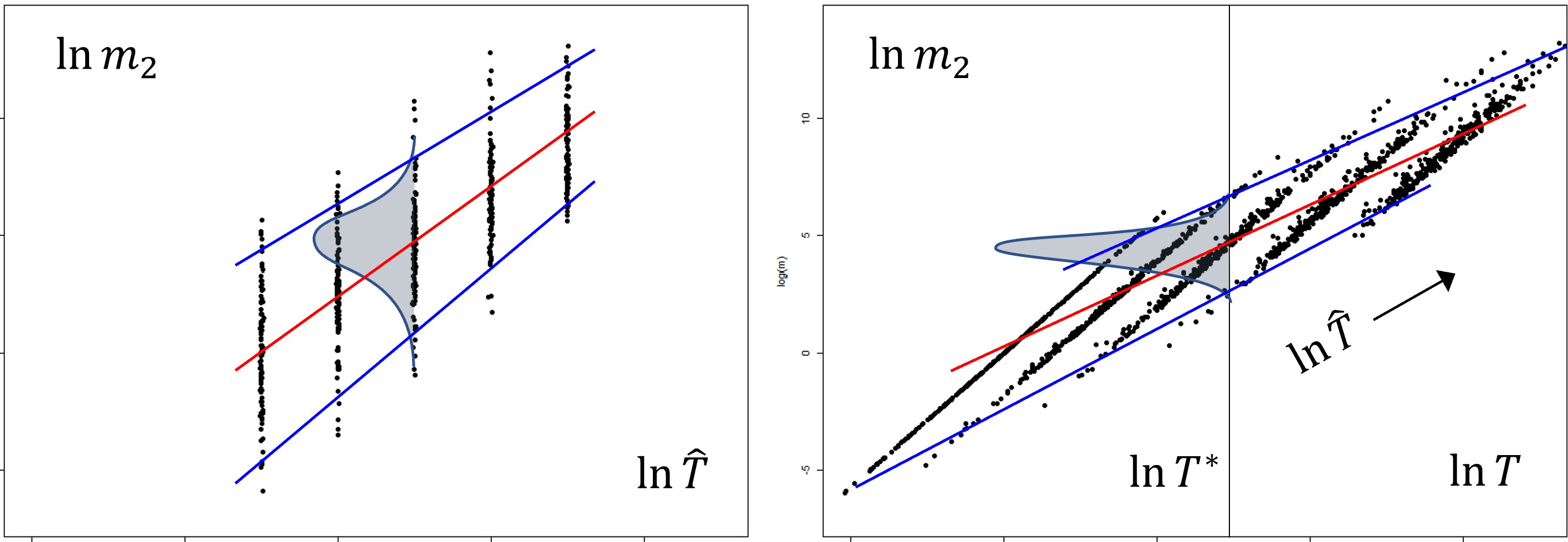
Fig. 1 (left) illustrates the situation based on a numerical simulation of for background times , measured in units of the time interval cutoff.
Red and blue lines connect the means and 5th/95th percentiles.
The variance of the distribution indeed decreases linearly in log-time, while its mean increases linearly.
The scatter plot fig. 1 (right) shows the bivariate distribution of and for the same values of .
The points indeed scatter around parallel, equidistant lines, reflecting the correlation of almost 1.
The moment at physical time is the expectation value of , restricted to paths , which lead to the end value :
Here, we must integrate over , which is a modulus of conformal gauge in 2+1 dimensions. The delta function cuts the bivariate distribution at a cross section of fixed physical time (the vertical line in fig. 1, right). The distribution along this cross section represents the stochastic process in physical time. It remains to read off its drift (the slope of the red “drift line” in fig. 1, right) and its standard deviation in the ansatz
| (25) |
where is Gaussian noise with variance 1. and are the “dressed” MRW parameters.
7 Gravitationally Dressed Hurst Exponents
The drift in physical time is easily inferred by combining the two equations (24):
This yields the parameter in ansatz (25) for the gravitationally dressed MRW:
| (26) |
We can determine the volatility of the noise in (25) from fig. 1 (right). From (21,22,23), the noise scatters around “noise lines” with slope . Its projection onto the cross section of fixed along the direction of the drift is the “gravitationally dressed” standard deviation of the noise. Geometrically, it is the difference of the slope of the “noise lines” and the slope of the “mean line”, expressed in physical log time . This yields the parameter
| (27) |
Note that and thus are uniquely determined by the central charge via relations (10). The Hurst exponents follow from (25) and Ito’s lemma:
| (28) |
They display multifractal scaling in physical time , decreasing linearly with .
This concludes the specification of the multifractal random walk in physical time.
Let us finally return to our scaling ansatz (13, 14). From the Hurst exponents (28), we determine the exponents in (14) such that they yield the correct scaling of the moments with physical time , and thereby also extract the scaling with the physical area :
| (29) |
The exponents contain a constant mono-scaling component and a multi-scaling component (linear in ). In particular, grows monotoneously, as runs from to .
8 Examples: Minimal Models
Let us illustrate our results with a few examples, based on the approximation (we leave it for future work to compute corrections). We consider the minimal models [20]. They are labelled by two co-prime integers (we choose ) and central charges
The unitary minimal models correspond to . For a given model, the primary fields are labelled by two integers (in place of ) and have dimensions
We put the minimal models on a genus zero random surface and obtain:
For the Ising model on a random surface with the magnetization as an order parameter (), the multiscaling effect is quite small, using formulas (26, 27):
This yields Hurst the exponents from (28):
As another example, the 3-state Potts model has a primary field (where ), which - if used as an order parameter - yields the parameters
One obtains a similar set of Hurst exponents from (28):
For the general unitary minimal models with and as an order parameter, one gets and obtains the Hurst exponents
The limit yields the Hurst exponents for models on a random surface [21]:
An interesting class of non-unitary minimal models are those with large negative central charge . Using the primary field as order parameter, one obtains in this limit:
Such models can be obtained by setting so
They can be interpreted as models with in the dense phase [22], and
include the Kazakov models and the topological models , which have no bulk fields, but have boundary fields
if one allows for world-sheet boundaries [22].
Let us conclude by noting that one would need , in order to explain the Hurst exponents that have been empirically observed in highly liquid financial markets (based on a wide range of estimates including [16, 17]). Within this rough approximation, this can be achieved by the Ising- and 3-states Potts models, as well as by other models including non-unitary ones, such as, e.g., the model. Precise empirical measurements and the search for a model that replicates all stylized facts of finance are in progress.
Acknowledgements
I would like to thank Henriette (formerly Wolfgang) Breymann, Uwe Täuber, and Matthias Staudacher for helpful discussions and Jean-Philippe Bouchaud for arising my interest in the multifractal random walk. This research is supported in part by the Swiss National Science Foundation under Practise-to-Science grant no. PT00P2_206333.
Appendix
Here, we derive the results quoted in section 6. The autocorrelation (6) of the Gaussian field of the MRW in background time is:
with correlation time . Physical time in (21) and the moments , viewed as stochastic processes (22) whose expectation value is , are defined as
| (30) | |||||
| (31) | |||||
| (32) |
To compute the Hurst exponents in physical time for the process shown in fig. 1, we need to know (i) the drifts, (ii) the variances,
and (iii) the covariances and correlations of the ”effective fields” as functions of .
We will calculate them for in the region , where our integrals converge,
and then analytically continue the results to general .
To compute the drift and variance of the Gaussian random variable , we first apply Ito’s lemma to the expectation values
is the variance of the effective field . Integrating (30) yields the relation
| (33) |
The simple solution turns out not to be the correct one. To see this, we derive a second relation between and by applying Ito’s lemma to :
| (34) |
On the other hand, inserting (30) for and performing the double integral yields
| (35) |
and is an integration constant. Here, self-contractions of at the same point have contributed two factors of . Combining (35) with (34) yields:
Together with (33), this yields the drift and variance of the effective field :
| (36) |
where we have defined the new constants . We see that the gravitational dressing gives physical log-time an additional drift
in background log-time , and a noise volatility that shrinks to 0 at the correlation time.
Analoguously, we compute the scaling of the mean and variance of in the second moment (31) for , once by using Ito’s lemma and once by performing the integrals:
| (37) | |||||
with integration constants . Generalizing this to yields the two equations
Combining them, one finds for the variances and drifts:
| (38) |
with new constants
We observe that the effective field has drift in log time. The variance of its noise shrinks linearly in log time and becomes zero at the correlation time,
analogously to that of .
Finally, we derive the covariance and correlation of and in an analogous manner:
| (39) |
On the other hand, inserting the three integrals in (30,31) for and yields the scaling
is another integration constant. Combining this with (39) and using (36,38) yields
The correlation is the covariance divided by the square roots of the two variances:
(the sign in the last equation must be negative as correlations are ).
We see that the deviation of the correlation of and from 1 is small for .
This also applies to the higher moments (we omit the derivation, which is completely analogous).
The integrals (35, 37) diverge at for and for , respectively. In the original 2+1-dimensional field theory, this is when the two random surfaces at coincide. These divergences mirror divergences that already occur in the “static limit”, i.e., in the 2-dimensional field theory of section 4 without the time dimension, when two operators at different points on the surface approach each other. In the renormalization process, these divergences are removed by counterterms. We assume that the renormalized moments are analytic functions and that our results, including formulas (26, 27, 28) of section 7, can be continued to general values of and . The same applies to the higher moments.
References
- [1] Polyakov, A. M. (1981). Quantum geometry of bosonic strings. Physics Letters B, 103(3).
- [2] Knizhnik, V. G., Polyakov, A. M., and Zamolodchikov, A. B. (1988). Fractal structure of 2d—quantum gravity. Modern Physics Letters A, 3(08), 819-826.
- [3] David, F. (1988). Conformal field theories coupled to 2-D gravity in the conformal gauge. Modern Physics Letters A, 3(17), 1651-1656. Distler, J., and Kawai, H. (1989). Conformal field theory and 2D quantum gravity. Nuclear physics B, 321(2), 509-527.
- [4] Seiberg, N. (1990). Notes on quantum Liouville theory and quantum gravity. Progress of Theoretical Physics Supplement, 102. Moore, G., Seiberg, N., & Staudacher, M. (1991). From loops to states in two-dimensional quantum gravity. Nuclear Physics B, 362(3).
- [5] Schmidhuber, Christof. ”Critical Dynamics of Random Surfaces: Time Evolution of Area and Genus.” arXiv preprint arXiv:2409.05547 (2024).
- [6] Schmidhuber, Christof. ”Financial Markets and the Phase Transition between Water and Steam.” Physica A: Statistical Mechanics and its Applications 592 (2022). Schmidhuber, Christof. ”Trends, reversion, and critical phenomena in financial markets.” Physica A: Statistical Mechanics and its Applications 566 (2021): 125642.
- [7] Hohenberg, P.C. and Halperin, B.I., 1977. Theory of dynamic critical phenomena. Reviews of Modern Physics, 49(3), p.435.
- [8] Täuber, Uwe C. Critical dynamics: a field theory approach to equilibrium and non-equilibrium scaling behavior. Cambridge University Press, 2014.
- [9] J. Zinn-Justin, Quantum Field Theory and Critical Phenomena, Oxford U. Press, 1989.
- [10] Gross, David J., and Alexander A. Migdal. ”A nonperturbative treatment of two-dimensional quantum gravity.” Nucl. Physics B 340.2-3 (1990). Gross, David J., and Alexander A. Migdal. ”Nonperturbative solution of the Ising model on a random surface.” Physical Review Letters 64.7 (1990): 717.
- [11] M. Douglas and S. Shenker, Nucl. Phys. B335, 635 (1990). E. Brezin and V. Kazakov, Phys. Lett. 236B, 144 (1990).
- [12] David, François. ”Phases of the large-N matrix model and non-perturbative effects in 2D gravity.” Nuclear Physics B 348.3 (1991). David, François. ”Non-perturbative effects in 2D gravity and matrix models.” Random Surfaces and Quantum Gravity. Boston, MA: Springer US, 1990. 21-33.
- [13] Bacry, Emmanuel, Jean Delour, and Jean-François Muzy. ”Multifractal random walk.” Physical review E 64.2 (2001): 026103.
- [14] Mandelbrot, B. B. (1974). Intermittent turbulence in self-similar cascades: divergence of high moments and dimension of the carrier. Journal of fluid Mechanics, 62(2). Mandelbrot, B. B., Fisher, A. J., & Calvet, L. E. (1997). A multifractal model of asset returns.
- [15] Ghashghaie, Shoaleh, et al. ”Turbulent cascades in foreign exchange markets.” Nature 381.6585 (1996): 767-770.
- [16] L. Borland, J.P. Bouchaud, J.F. Muzy, G. Zumbach (2005). The Dynamics of Financial Markets - Mandelbrot’s multifractal cascades and beyond. arXiv: cond-mat/ 0501292.
- [17] Di Matteo, Tiziana. ”Multi-scaling in finance.” Quantitative finance 7.1 (2007).
- [18] Francesco, Philippe, Pierre Mathieu, and David Sénéchal. Conformal field theory. Springer Science & Business Media, 2012.
- [19] Schomerus, Volker. ”Non-compact string backgrounds and non-rational CFT.” Physics reports 431.2 (2006): 39-86.
- [20] Belavin, A. A., Polyakov, A. M., & Zamolodchikov, A. B. (1984). Infinite conformal symmetry in two-dimensional quantum field theory. Nuclear Physics B, 241(2), 333-380.
- [21] Review arcticle: Klebanov, I. R. (April 1991). String theory in two-dimensions. In Spring School on string theory and quantum gravity, Trieste, Italy (pp. 30-101).
- [22] Kostov, Ivan K., and Matthias Staudacher. ”Multicritical phases of the O (n) model on a random lattice.” Nuclear Physics B 384.3 (1992): 459-483.