Point-MoE: Towards Cross-Domain Generalization in 3D Semantic Segmentation via Mixture-of-Experts

Abstract

While scaling laws have transformed natural language processing and computer vision, 3D point cloud understanding has yet to reach that stage. This can be attributed to both the comparatively smaller scale of 3D datasets, as well as the disparate sources of the data itself. Point clouds are captured by diverse sensors (e.g., depth cameras, LiDAR) across varied domains (e.g., indoor, outdoor), each introducing unique scanning patterns, sampling densities, and semantic biases. Such domain heterogeneity poses a major barrier towards training unified models at scale, especially under the realistic constraint that domain labels are typically inaccessible at inference time. In this work, we propose Point-MoE, a Mixture-of-Experts architecture designed to enable large-scale, cross-domain generalization in 3D perception. We show that standard point cloud backbones degrade significantly in performance when trained on mixed-domain data, whereas Point-MoE with a simple top-$k$ routing strategy can automatically specialize experts, even without access to domain labels. Our experiments demonstrate that Point-MoE not only outperforms strong multi-domain baselines but also generalizes better to unseen domains. This work highlights a scalable path forward for 3D understanding: letting the model discover structure in diverse 3D data, rather than imposing it via manual curation or domain supervision.

1 Introduction

In both language and vision, we have witnessed remarkable advances driven by two trends: the aggregation of massive heterogeneous datasets Schuhmann et al. (2022); Sun et al. (2017); Bain et al. (2021); Raffel et al. (2023); Byeon et al. (2022); Zhou et al. (2022), and the deployment of models of ever-increasing capacity trained on them in a unified manner Brown et al. (2020); Chowdhery et al. (2022); Radford et al. (2021a); Kirillov et al. (2023); Dosovitskiy et al. (2021); Oquab et al. (2023). These models succeed not because they were crafted for a specific domain, but because they were trained to learn underlying patterns across a wide variety of datasets. However, 3D point cloud understanding has yet to follow the same trajectory of progress, despite its wide applications in roboticsChen et al. (2023); Peri et al. (2024); Ze et al. (2024), autonomous systemsChen et al. (2017, 2020); Li et al. (2020), augmented realityZieliński et al. (2024); Weber et al. (2024), and embodied intelligenceWijmans et al. (2019); Wang et al. (2023). Taking the 3D semantic segmentation task as an example, although diverse 3D datasets exist—such as ScanNet Dai et al. (2017), SemanticKITTI Behley et al. (2019a), nuScenes Caesar et al. (2020), and ASE Avetisyan et al. (2024)—each covers only a narrow subset of the real-world diversity in 3D assets. Point clouds are generated from a variety of pipelines: RGB-D sensors Chang et al. (2017), terrestrial and airborne LiDAR Henrich et al. (2024); Puliti et al. (2023), and multi-view stereo Yao et al. (2020). Each source brings its own characteristics—differing point densities, coverage patterns, reconstruction artifacts, and semantic biases (Fig. 1 left). The result is a 3D ecosystem of rich, yet siloed data sources, where models trained in one silo often fail to generalize across others.

A natural response to address this challenge is to train across such silos. For example, one might naively train the state-of-the-art Point Transformer V3 (PTv3) Wu et al. (2024a) (Fig. 1a) on mixed-domain 3D datasets. However, such models struggle to reconcile heterogeneous characteristics of the data, even with increased network capacity (Tab. 1). To mitigate this, recent methods introduce domain-aware components. Point Prompt Training (PPT) Wu et al. (2024b) (Fig. 1b) modifies PTv3 by assigning domain-specific normalization layers. Similarly, One-for-All Wang et al. (2024b) achieves improved 3D detection performance by employing a lightweight classifier to infer dataset labels, then applying domain-specific adapters. While these methods show notable gains, they rely on access to domain labels during training and exhibit performance degradation on unseen domains. A likely cause is that adapting only the normalization parameters may be insufficient to fully capture the complex variations required for scalable, cross-domain generalization.

In this work, we hypothesize that Mixture-of-Experts (MoE) architectures Jacobs et al. (1991); Jordan and Jacobs (1993) are well-suited for cross-domain joint training. We introduce Point-MoE, a sparse MoE model built upon PTv3 Wu et al. (2024a). As illustrated in Fig. 1c, Point-MoE replaces each feed-forward layer in PTv3 with a MoE layer comprising of multiple expert networks (implemented as feed-forward MLPs) and a router that dynamically selects a sparse subset of experts for each input token. Our design is motivated by three key insights. First, MoE provides a natural inductive bias for handling diverse inputs by encouraging expert specialization and learning token-to-expert routing Chirkova et al. (2024); Xu et al. (2025). This allows a single model to be trained on mixed-domain data without requiring access to domain labels. Second, compared to normalization-based domain adaptation methods like PPT Wu et al. (2024b) and One-For-All Wang et al. (2024b), MoE offers a significantly larger and more expressive representation space, enabling better modeling of domain-specific variations. Third, sparse MoE architectures improve computational efficiency during both training and inference, and have emerged as a standard design for scaling large models Lepikhin et al. (2020); Fedus et al. (2022); Du et al. (2022); Riquelme et al. (2021); Dai et al. (2024). We extend these empirical benefits of MoE, previously established in language and vision, to the domain of 3D point cloud understanding, with a particular focus on 3D semantic segmentation.

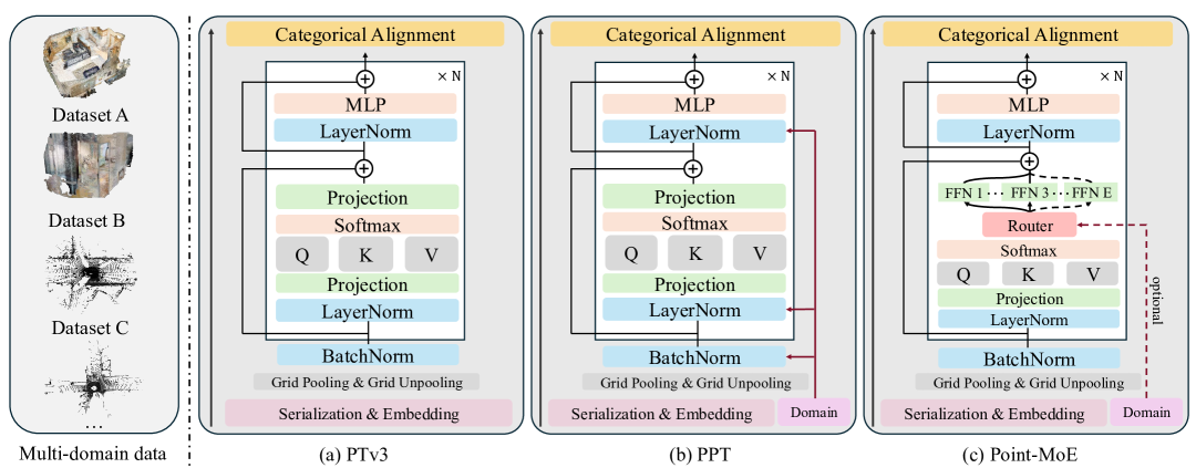
Figure 1: Overview of cross-domain training architectures. Point clouds exhibit diverse characteristics across domains. (a) Naively training Point Transformer V3 (PTv3) Wu et al. (2024a) on multi-domain data leads to degraded performance within each domain. (b) Point Prompt Training (PPT) Wu et al. (2024b) addresses this by adding domain-aware normalization parameters. (c) Our proposed Point-MoE tackles this challenge with Mixture-of-Experts (MoE), enabling dynamic expert specialization across domains. Domain labels can optionally be provided to the router to guide the expert selection.

We conduct extensive experiments across a diverse mixture of 3D datasets, spanning indoor and outdoor scenes, synthetic and real data, and multiple sensor types. To comprehensively assess the effectiveness of Point-MoE, we evaluate it under both domain-agnostic (i.e., without access to domain labels) and domain-aware training regimes. Our results show that Point-MoE consistently adapts well to both settings, achieving strong generalization to unseen domains while outperforming competitive baselines, with improved training (Fig. 2) and inference efficiency (Tab. 1 and 2). We also conduct a thorough ablation study analyzing key design choices, including the number of experts, sparsity level, and the placement of MoE layers (Tab. 3). Remarkably, even without domain supervision, Point-MoE learns to route input data meaningfully and to specialize experts organically—emerging from the data distribution itself (Fig. 3 and 4).

To the best of our knowledge, this work presents the first systematic exploration of the Mixture-of-Experts architecture for 3D point cloud understanding in the context of cross-domain generalization. These findings point toward a scalable path forward for 3D perception: instead of designing separate models for each dataset or domain, we should aim to develop unified systems that can adapt across the full spectrum of 3D data sources. In this regard, Point-MoE emerges as a promising and flexible framework for bridging domain gaps in large-scale 3D semantic segmentation.

2 Related Work

Point Cloud understanding.

Deep learning backbones for 3D scene understanding can be broadly categorized by how they process point clouds: projection-based methods Chen et al. (2017); Lang et al. (2019); Li et al. (2016); Su et al. (2015), voxel-based methods Maturana and Scherer (2015); Song et al. (2016); Choy et al. (2019); Graham et al. (2017), and point-based methods Qi et al. (2017a, b); Thomas et al. (2019); Zhao et al. (2019). More recently, transformer-based architectures operating on point clouds have emerged as strong contenders in this space Guo et al. (2021); Wu et al. (2022); Zhao et al. (2021); Wu et al. (2024a). Among them, Point Transformer V3 (PTv3) Wu et al. (2024a) represents the current state of the art, introducing a novel space-filling curve based serialization scheme, that transforms the unstructured 3D points into a 1D sequence, enabling efficient transformer-based modeling. A recent series of works have explored scaling such point cloud models to the multi-dataset setting using domain-aware training strategies. Point Prompt Training (PPT)  Wu et al. (2024b) demonstrates that using domain-specific normalization layers during pretraining improves 3D segmentation performance across multiple datasets. In 3D detection, One-for-All Wang et al. (2024b) adopts a sparse convolutional network with domain-specific partitions and normalization layers to boost multi-domain performance. Rather than relying on such domain-specific architectural branches Wu et al. (2024b); Wang et al. (2024b), we propose a unified sparse expert framework that learns to specialize dynamically across various domains, without requiring explicit dataset labels during training or inference.

Mixture-of-Experts.

Mixture-of-Experts (MoE) Jacobs et al. (1991); Jordan and Jacobs (1993) aims to increase model capacity without a proportionate increase in compute costs by levereaging conditional computation – large portions of the model are only activated conditioned on certain input samples Shazeer et al. (2017). In NLP, MoE has enabled scaling up models from hundreds of millions to hundreds of billions (and beyond) parameters: GShard scales to 600 B parameters Lepikhin et al. (2020), Switch Transformer to 1.6 T parameters Fedus et al. (2022), ST-MoE to 260 B parameters Zoph et al. (2022), and GLaM to 1.2 T parameters Du et al. (2022), all at roughly the same training cost as a dense model one-tenth the size. V-MoE Riquelme et al. (2021) applies this recipe to vision, demonstrating competitive accuracy at 15 B parameters with batch-priority routing. More recently, Mixtral 8x7B Jiang et al. (2024) and DeepSeek models Dai et al. (2024); DeepSeek-AI et al. (2024, 2025) all employ Mixture-of-Experts for large language model pretraining.

Apart from being a powerful tool for scaling up model capacity, MoE is well-suited to training on data drawn from heterogeneous domains, because the experts naturally tend to self-organize on a per-domain basis. Early work shows gains in multi-source sentiment and POS tagging Guo et al. (2018), domain-adaptive language modeling Gururangan et al. (2021), automatic chart understanding Xu et al. (2025), and multilingual translation Chirkova et al. (2024). Mod-Squad Chen et al. (2022) introduces a modular mixture-of-experts framework for multi-task learning, optimizing task-expert matching to balance cooperation and specialization across tasks. DAMEX Jain et al. (2023) applies this to visual domains, while MoE-LLaVA Lin et al. (2024), DeepSeek-VL Lu et al. (2024), and DeepSeek-VL 2 Wu et al. (2024c) report similar benefits in vision-language models. To our knowledge, ours is the first attempt at extending MoE to address multi-dataset training and cross-domain generalization for 3D point clouds.

3 Point-MoE for Cross-Domain Point Cloud Understanding

Task definition. Given a 3D scene represented as a point cloud $\mathcal{P}=\{p_{i}\}_{i=1}^{n}$, where each point $p_{i}\in\mathbb{R}^{3}$ denotes coordinates, semantic segmentation aims to predict a single class label $\hat{y}_{i}\in\mathcal{C}$ to each point $p_{i}$ from a fixed label set $\mathcal{C}=\{c_{1},c_{2},\ldots,c_{m}\}$. Multi-domain data are utilized during training. Let the domain containing $N$ point clouds be $\mathcal{D}=\mathopen{}\mathclose{{\left\{\mathopen{}\mathclose{{\left(p_{i},y_{i}}}\right)_{i=1}^{n}}}\right\}^{N}$. Then the complete training set across $d$ domains can be represented as: $\mathopen{}\mathclose{{\left\{\mathcal{D}_{k}}}\right\}_{k=1}^{d}$. The goal of multi-domain joint training is to learn a unified model over all domains that minimizes prediction error across $\mathopen{}\mathclose{{\left\{\mathcal{D}_{k}}}\right\}$, while also generalizing effectively to domains unseen during training.

We adopt a minimal Mixture-of-Experts design that closely follows the standard architecture prevalent in the recent NLP literature. This simplicity allows us to leverage existing scalable Transformer-based MoE implementations with minimal modification. For the base model, we use Point Transformer V3 (PTv3) Wu et al. (2024a), a state-of-the-art architecture for point cloud understanding. Below we introduce the architecture of Point-MoE in detail.

Mixture-of-Experts layer. The core of MoE is to route input tokens dynamically to specialized subnetworks, referred to as experts, via a lightweight gating mechanism. Given an input feature vector $\mathbf{x}\in\mathbb{R}^{d}$, each MoE layer contains $N$ experts $\{f_{i}\}_{i=1}^{N}$ and a gating network $G:\mathbb{R}^{d}\rightarrow\mathbb{R}^{N}$. For each input $\mathbf{x}$, the MoE layer output is computed as a weighted sum over the top-$k$ activated experts:

$$\mathrm{MoE}(\mathbf{x})=\sum_{i\in\mathcal{S}_{\mathbf{x}}}G_{i}(\mathbf{x})f_{i}(\mathbf{x})$$ (1)

where $\mathcal{S}_{\mathbf{x}}$ denotes the set of top-$k$ experts selected for input $\mathbf{x}$, and $G_{i}(\mathbf{x})$ represents the normalized gating weight assigned to expert $i$. In practice, the gating function is typically implemented via a linear projection followed by a sparse softmax, ensuring activation of only a small subset of experts, with $k\ll N$. Although auxiliary losses for balancing expert load are common in prior work Shazeer et al. (2017), we empirically observed them to be unnecessary and therefore excluded them from our final setup.

Integration into PTv3. To tailor the MoE architecture specifically for 3D point cloud data, we integrate the MoE mechanism directly into PTv3 by replacing the shared linear projection layers in PTv3’s attention module with an MoE layer. The original linear projections mapping input features into key, query, and value vectors within the attention mechanism are replaced by MoE layers, while all subsequent computations remain unchanged. This integration allows the MoE experts to specialize naturally in domain-specific transformations of point cloud data. Fig. 1c provides a visual overview of the modified architecture. It is crucial to insert the MoE layer before the post-normalization; otherwise, we observe a significant reduction in performance gains.

Language-guided classification. To bridge label discrepancies across datasets, we project per-point features to a shared language space using CLIP Radford et al. (2021b) text embeddings, following PPT Wu et al. (2024b). This enables supervision via class names, without relying on dataset labels. For instance, the class “pillow” is missing in ScanNet (grouped as “other”) but is explicitly labeled in Structured3D. Our model aligns point features with the CLIP Radford et al. (2021b) embedding of “pillow,” allowing knowledge to transfer across domains even in the absence of direct supervision.

Domain-aware gating. Our preliminary experiments show that while basic Point-MoE naturally specializes experts implicitly, providing explicit domain information could further guide and accelerate expert specialization. To explore this, we introduce a dataset-aware gating variant termed Domain-Aware Point-MoE. In this variant, we explicitly associate each training domain $\mathcal{D}_{i}$ with a unique, learnable domain embedding vector $d_{i}\in\mathbb{R}^{d}$. Before routed through the gating mechanism, each input feature $x_{t}$ is concatenated with the corresponding domain embedding: $G_{t}(d)=\mathrm{softmax}(W\cdot(x_{t}\oplus d_{i}))$, where $W$ denotes a learnable linear projection, and the concatenation operation explicitly conditions gating decisions on the domain identity. This explicit conditioning encourages faster and more clearly delineated expert specialization aligned with dataset-specific characteristics observed during training.

Domain randomization for robust gating. While domain-aware gating allows experts to specialize based on known domain identities, this approach assumes access to explicit domain labels at inference time. In practical scenarios, such labels are often unavailable—especially when deploying models in the wild, where domain boundaries may be ambiguous or entirely unknown. While a domain detector can be employed to approximate the domain label by mapping unseen domains to the closest known ones, such detectors may introduce errors or fail to capture nuanced domain shifts. This motivates the need for a more robust mechanism that does not rely on explicit domain identification at test time. To address this, we introduce a domain randomization strategy that enables the model to generalize to unseen or mixed-domain inputs without performance degradation on seen domains.

Specifically, we define a learnable generic domain embedding and randomly assign it to 20% of the training points, replacing their true domain-specific embeddings. This forces the gating mechanism to learn domain-agnostic routing behavior, even in the presence of domain ambiguity. The remaining 80% of points retain their original domain embeddings, ensuring that the model still benefits from explicit supervision where available. In line with prior work Wang et al. (2022); Chirkova et al. (2024), we find that domain randomization improves generalization to unseen domains while preserving strong performance on those seen during training.

Training objective. We use Mixture-of-Experts (MoE) in a supervised cross-domain setting, where the goal is to train a unified model $f(x;\theta)$ across $n$ domains $\{\mathcal{D}_{i}\}_{i=1}^{n}$, each containing samples $(X,Y)\sim\mathcal{D}_{i}$. The objective is to minimize the average loss across domains:

$$\min_{\theta}\sum_{i=1}^{n}\mathbb{E}_{(X,Y)\sim\mathcal{D}_{i}}\;\mathcal{L}(f(X;\theta),Y)$$ (2)

We consider two batching strategies during training: (1) Single-domain batching, where each batch is sampled from only one domain $\mathcal{D}_{i}$ at a time. (2) Mixed-domain batching, where each batch contains samples from multiple domains. Our implementation is based on the official open-source code of PTv3 released by Pointcept Contributors (2023).

4 Experiments

We conduct comprehensive experiments to evaluate Point-MoE for cross-domain 3D semantic segmentation. First, we describe baseline methods and experimental setups (Sec. 4.1). Then, we present detailed empirical results under two primary joint training scenarios: (1) indoor-only, and (2) combined indoor-outdoor training (Sec. 4.2). Finally, we provide ablation studies that highlight key design choices of the MoE architecture (Sec. 4.3) and detailed analysis of MoE behaviors (Sec. 4.4).

4.1 Experimental Setup

Baseline methods. Since our proposed Point-MoE framework is built upon PTv3 Wu et al. (2024a), we adopt PTv3 and PPT Wu et al. (2024b) as primary baselines. PPT, originally designed for dataset-specific BatchNorm  Ioffe and Szegedy (2015) and LayerNorm Ba et al. (2016) layers and fine-tuning, is adapted here for joint training. Because PPT requires dataset labels at inference time, we follow One-for-All Wang et al. (2024b) to train a lightweight domain classifier (achieving over 95% accuracy), which we also use for Point-MoE under the domain-aware setting.

To ensure a fair comparison, we begin by benchmarking the dense PTv3 model under the domain-agnostic joint training setting, systematically varying key design factors such as mixed-batch composition and normalization strategy. In this setup, models are trained across multiple domains without access to dataset labels, and no label information is provided at inference time. This setting reflects a realistic deployment scenario where domain metadata is unavailable. For the domain-aware joint training setting, we compare to the PPT + One-for-All baseline. Here, models are trained with access to dataset labels. During inference, we either provide predicted labels using a trained domain classifier or assign a “generic” class to simulate deployment in unknown or mixed domains. This allows us to isolate the value of domain conditioning and assess the robustness of Point-MoE under both domain-aware and domain-agnostic regimes.

Datasets. Experiments are conducted on three indoor datasets—ScanNet Dai et al. (2017), S3DIS Armeni et al. (2016), and Structured3D Zheng et al. (2020)—and evaluated on both seen and unseen domains, including Matterport3D Chang et al. (2017). We then evaluate the best-performing Point-MoE and baseline configurations under a more challenging indoor-outdoor setting, incorporating outdoor datasets from nuScenes Caesar et al. (2020), SemanticKITTI Behley et al. (2019b), and Waymo Sun et al. (2020). Voxel sizes are standardized to 0.02m for indoor scenes and 0.05m for outdoor scenes. Throughout, we denote model capacity using -S (small) and -L (large) suffixes for all architectures, including PTv3, Point-MoE, and PPT.

4.2 Experimental Results

Table 1: Performance of Joint Training for Indoor 3D Semantic Segmentation. All models are jointly trained on three indoor datasets and evaluated under two settings. In Domain-agnostic joint training, models are evaluated using only the point cloud and the corresponding dataset-specific label set. In Domain-aware joint training, a predicted scene label from a domain classifier is provided at inference time to guide the model. “-G” indicates that model utilizes domain randomization and contains a learnable “generic” domain label during training. All results are reported as mean Intersection-over-Union (mIoU).

Methods	Params	Activated	Mix	Layer.	ScanNet	Structured3D		S3DIS	Matterport3D
					Seen				Unseen
					Val	Val	Test	Val	Val	Test
Single-dataset training
PTv3-ScanNet Wu et al. (2024a)	46M	46M			75.0	19.8	20.9	8.8	38.9	44.5
PTv3-Structured3D Wu et al. (2024a)	46M	46M			21.2	81.5	79.4	7.1	21.0	24.0
PTv3-S3DIS Wu et al. (2024a)	46M	46M			4.9	3.5	5.3	67.6	5.0	3.4
PTv3-Matterport3D Wu et al. (2024a)	46M	46M			53.1	22.9	23.7	9.8	54.1	56.0
Domain-agnostic joint training
(1) PTv3-S Wu et al. (2024a)	46M	46M			50.3	63.0	60.9	44.5	lightblue29.1	lightblue37.1
(2) PTv3-S Wu et al. (2024a)	46M	46M	✓		69.7	47.9	50.3	64.7	lightblue36.6	lightblue42.6
(3) PTv3-S Wu et al. (2024a)	46M	46M	✓	✓	71.3	56.6	55.9	69.4	lightblue37.7	lightblue44.1
(4) PTv3-L Wu et al. (2024a)	97M	97M			58.7	61.6	60.8	42.4	lightblue32.8	lightblue39.7
(5) PTv3-L Wu et al. (2024a)	97M	97M	✓		74.6	60.8	59.7	69.1	lightblue40.2	lightblue46.6
(6) PTv3-L Wu et al. (2024a)	97M	97M	✓	✓	72.2	56.0	58.1	67.4	lightblue39.0	lightblue45.4
(7) Point-MoE-S	59M	52M	✓		75.4	69.2	69.7	67.7	lightblue41.9	lightblue46.8
(8) Point-MoE-L	100M	59M	✓		75.8	73.0	67.9	68.4	lightblue41.6	lightblue47.8
Domain-aware joint training
(9) PPT-S Wu et al. (2024b); Wang et al. (2024b)	47M	47M			74.7	64.2	65.5	64.7	lightblue27.6	lightblue26.1
(10) PPT-L Wu et al. (2024b); Wang et al. (2024b)	98M	98M			74.7	64.9	65.8	62.0	lightblue27.8	lightblue26.3
(11) Point-MoE-S	59M	52M	✓		76.7	66.7	72.2	64.1	lightblue29.8	lightblue30.5
(12) Point-MoE-L	100M	59M	✓		75.6	69.6	71.3	69.6	lightblue41.1	lightblue49.1
(13) Point-MoE-G-S	59M	52M	✓		75.7	69.1	70.9	62.1	lightblue41.1	lightblue47.2
(14) Point-MoE-G-L	100M	59M	✓		76.7	68.0	69.6	67.0	lightblue41.8	lightblue47.8

Table 2: Cross-domain 3D Semantic Segmentation across Indoor and Outdoor Scenes. We evaluate the best-performing models from the indoor-only setting in a more challenging joint training setup that spans both indoor and outdoor datasets. This setup better reflects real-world deployment scenarios, requiring models to generalize across diverse domains.

ScanNet

Structured3D

S3DIS

nuScenes

SemKITTI

Matterport3D

Waymo

Indoor

Outdoor

Indoor

Outdoor

Seen

Unseen

Methods

Params

Activated

Mix

Layer.

Val

Val

Test

Val

Val

Val

Val

Test

Val

Test

Domain-agnostic joint training

(1) PTv3 Wu et al. (2024a)

97M

97M

56.6

49.0

52.1

19.1

45.5

35.9

lightblue28.7

lightblue41.4

lightblue12.2

lightblue12.6

(2) PTv3 Wu et al. (2024a)

97M

97M

✓

77.1

63.3

63.7

61.6

70.3

65.4

lightblue40.7

lightblue46.3

lightblue23.6

lightblue25.2

(3) PTv3 Wu et al. (2024a)

97M

97M

✓

✓

74.6

64.1

63.9

68.0

69.6

62.9

lightblue39.1

lightblue45.9

lightblue21.9

lightblue23.2

(4) Point-MoE-L

100M

59M

✓

76.2

69.5

70.2

67.8

72.9

63.2

lightblue41.3

lightblue49.6

lightblue23.7

lightblue25.3

Domain-aware joint training

(5) PPT-L Wu et al. (2024b)

98M

98M

76.7

67.5

66.0

61.9

70.8

66.9

lightblue24.9

lightblue23.1

lightblue16.3

lightblue16.7

(6) Point-MoE-L

100M

59M

✓

76.8

67.5

70.1

61.4

72.2

64.2

lightblue22.9

lightblue23.8

lightblue18.6

lightblue19.2

(7) Point-MoE-G-L

100M

59M

✓

77.0

72.1

74.2

62.4

72.7

64.4

lightblue38.8

lightblue44.8

lightblue24.8

lightblue26.2

Single-dataset training. We begin by evaluating the standard setting in which models are trained and evaluated on individual datasets. Note we train end evaluate PTv3 with language-guided classification. As shown in Tab. 1, PTv3 achieves strong in-domain performance, but its performance drops significantly on unseen domains. For instance, a PTv3 model trained on S3DIS achieves only 3.5% on Structured3D and 4.9% on ScanNet. While domain-specific models are not expected to generalize across domains or categories, these results underscore the brittleness of single-dataset training. This motivates the need for cross-domain training strategies that expose the model to diverse data and promote broader generalization.

Domain-agnostic joint training. In the indoor-only setting, Point-MoE outperforms all variants of PTv3 in most domains and performs competitively on S3DIS. Referring to Tab. 1, Point-MoE-S achieves 75.4% on ScanNet and 69.7% on S3DIS, outperforming PTv3-S by +4.1% and +13.8%, respectively. Remarkably, Point-MoE-S activates only 52M parameters compared to 97M in PTv3-L, yet still surpasses PTv3-L by +0.8% on ScanNet and +8.4% on S3DIS. In addition, Point-MoE-L reaches 75.8% on ScanNet and 73.0% on Structured3D, significantly ahead of PTv3-L. On the unseen Matterport3D domain, Point-MoE-L obtains 41.6% on validation set and 47.8% on test set, outperforming PTv3-L by +1.4% and +1.2% respectively while activating only 59M parameters at inference. In the more challenging indoor and outdoor setting, Point-MoE-L again leads across the board with a few being competitve. Referring Tab. 2, Point-MoE-L achieves 69.2% on S3DIS validation and 70.2% on test split, outperforming the best dense baseline by +5.4% and +6.3%, respectively. On outdoor datasets, Point-MoE-L achieves 72.9% on nuScenes exceeding the dense baseline by +2.6%. Notably, on the unseen datasets, Point-MoE-L outperforming all dense PTv3 variants by a clear margin. These gains are achieved while activating nearly half the parameters of PTv3-L, underscoring the efficiency and scalability of sparse expert routing.

Domain-aware joint training. We further evaluate Point-MoE in the domain-aware setting, where models are trained with access to dataset labels. In the indoor-only setting, both domain-aware Point-MoE and its generic variant (Point-MoE-G) surpass all strong baselines: variants of PPT Wu et al. (2024b) + One-for-All Wang et al. (2024b). As shown in Tab. 1, Point-MoE-G-L achieves 76.7% on ScanNet, 68.0% on Structured3D, and 67.0% on S3DIS, outperforming the best PPT + One-for-All baseline by +2.0%, +3.1%, and +2.3%, respectively. On the unseen Matterport3D dataset, it reaches 41.8% on the validation split and 47.8% on the test set, again outperforming all baselines. Notably, using only 20% of training data tagged as “generic” does not degrade performance on seen domains.

In the indoor-and-outdoor setting, Point-MoE-G-L continues to outperform all baselines across the board. Referring to Tab. 2, it achieves 77.0% on ScanNet, 72.1% and 74.2% on Structured3D (val/test), 62.4% on S3DIS and 72.7% on nuScenes—surpassing the best baseline by +0.3%, +4.6%, +4.1%, +1.0% and +0.5%, respectively. On the unseen domains, including Matterport3D and Waymo, Point-MoE-G-L delivers the strongest generalization. Crucially, it performs on par with domain-aware Point-MoE on seen datasets while achieving superior accuracy on unseen ones. These results validate that domain randomization with a generic label can enhance robustness without compromising in-domain performance. We still observe a performance gap between cross-domain and single-dataset training in cases like Structured3D Zheng et al. (2020). Single-dataset models can adapt to domain-specific cues and distributions, while Point-MoE must balance capacity across domains. As a result, its performance may trail on large, homogeneous datasets, but remains competitive overall due to its generalization ability.

4.3 MoE Design Ablation

Table 3: Ablation of Point-MoE Design and Hyperparameters. We conduct a systematic ablation on key design and hyperparameter choices of Point-MoE across four indoor multi-domain datasets: ScanNet (Scan), Structured3D (S3D), S3DIS, and Matterport3D (Mat).

$\alpha$	Scan	S3D	S3DIS	[HTML]EFEFEFMat
$0$	[HTML]EFEFEF74.5	[HTML]EFEFEF66.9	[HTML]EFEFEF68.6	[HTML]EFEFEF40.1
$10^{-4}$	72.3	64.1	67.9	39.5
$10^{-3}$	71.6	58.8	67.4	37.4

(a) Auxiliary load balancing loss. Removing the auxiliary loss consistently improves performance.

top $k$	Scan	S3D	S3DIS	[HTML]EFEFEFMat
top 1	74.4	64.8	65.5	39.0
top 2	[HTML]EFEFEF74.5	[HTML]EFEFEF66.9	[HTML]EFEFEF68.6	[HTML]EFEFEF40.1
top 3	73.8	62.4	67.8	39.7

(b) Top-$k$ expert selection. Best performance is achieved with $k{=}2$ experts.

norm	Scan	S3D	S3DIS	[HTML]EFEFEFMat
BN.	[HTML]EFEFEF74.5	[HTML]EFEFEF66.9	[HTML]EFEFEF68.6	[HTML]EFEFEF40.1
LN.	70.8	56.9	67.3	37.2
RMS.	45.3	36.5	51.1	24.6

(c) Normalization. BatchNorm yields strongest performance; RMSNorm degrades results.

case	Scan	S3D	S3DIS	[HTML]EFEFEFMat
dec.	74.0	64.9	66.6	38.1
all	[HTML]EFEFEF74.5	[HTML]EFEFEF66.9	[HTML]EFEFEF68.6	[HTML]EFEFEF40.1

(d) MoE position. Inserting MoE in all layers yields the best results.

act.	Scan	S3D	S3DIS	[HTML]EFEFEFMat
SiLU	73.6	65.7	64.9	[HTML]EFEFEF40.1
ReLU	[HTML]EFEFEF74.5	[HTML]EFEFEF66.9	[HTML]EFEFEF68.6	[HTML]EFEFEF40.1

(e) Activation functions. ReLU performs the best.

case	Scan	S3D	S3DIS	[HTML]EFEFEFMat
1H	73.0	[HTML]EFEFEF60.3	[HTML]EFEFEF66.3	39.5
2H	[HTML]EFEFEF73.5	58.6	65.4	[HTML]EFEFEF39.8

(f) Expert width. H indicates original feature dimension.

shared	Scan	S3D	S3DIS	[HTML]EFEFEFMat
0	[HTML]EFEFEF74.5	[HTML]EFEFEF66.9	[HTML]EFEFEF68.6	[HTML]EFEFEF40.1
1	73.6	62.3	66.6	39.1

(g) Shared experts. Not sharing experts yields better performance.

num.	Scan	S3D	S3DIS	[HTML]EFEFEFMat
4	[HTML]EFEFEF74.5	66.9	[HTML]EFEFEF68.5	40.1
8	73.6	[HTML]EFEFEF68.7	[HTML]EFEFEF68.5	[HTML]EFEFEF40.4

(h) Number of experts. More experts improve performance.

batch	Scan	S3D	S3DIS	[HTML]EFEFEFMat
4	74.0	64.9	66.6	38.1
6	[HTML]EFEFEF74.3	[HTML]EFEFEF66.9	[HTML]EFEFEF68.6	[HTML]EFEFEF40.1

(i) Batch size. Larger batchsize improves performance.

We investigate the impact of MoE design choices and hyper-parameters choices in indoor cross-domain 3D semantic segmentation. All experiments are conducted with ScanNet Dai et al. (2017), Structured3D Zheng et al. (2020) and S3DIS Armeni et al. (2016) and evaluate without providing dataset label on seen dataset and also evaluate on unseen dataset: Matterport3D Chang et al. (2017). Results are presented in Tab. 3.

Auxiliary load-balancing loss. The auxiliary load-balancing loss is designed to encourage uniform expert usage and prevent expert collapse Qiu et al. (2025); Wei et al. (2024); Li et al. (2024). We ablate its effect by training models with varying strengths of this loss in Tab. 3. Interestingly, we find that removing the auxiliary loss entirely leads to consistently better performance across domains. In contrast, stronger auxiliary losses result in significant degradation. We hypothesize that this is due to the inherent imbalance in the distribution of samples across domains in 3D point cloud datasets—a phenomenon also observed by ChartMoE Xu et al. (2025).

Effect of activated experts. Tab. 3 compares the performance of configurations with 1, 2 and 3 activated experts, finding diminishing return when increasing number of activated experts. We find that activating two experts yields the best performance across domains. This analysis suggests that merely increasing the number of activated experts does not guarantee improved performance.

MoE position. We ablate the placement of MoE layers to understand where expert specialization is most effective. Empirically, we observe greater expert diversity when MoE is applied in the decoder compared to the encoder. In Tab. 3, we compare two configurations: applying MoE layers only in the decoder, versus applying them in both the encoder and decoder. Results show that applying MoE to both stages consistently yields better performance, suggesting that expert specialization benefits from exposure to both encoder and decoder.

Effect of scaling model with MoE. Tab. 3 compares Point-MoE with 4 and 8 experts with activated experts fixed at 2. Increasing the number of experts from 4 to 8 leads to improved performance on seen domains, and yields a modest gain of 0.4% on the unseen domain. Tab. 3 ablates the expert width by varying the intermediate size of the MLP (e.g., 1H, 2H). The results show a mixed trend: wider experts improve performance on ScanNet and Matterport3D, but degrade results on Structured3D and S3DIS. Finally, we investigate the effect of adding shared experts Su et al. (2025); Wang et al. (2024a); Dai et al. (2024), which are applied universally without gating. We find that disabling shared experts consistently leads to better accuracy and domain specialization across all benchmarks, as reported in Tab. 3.

Ablation of hyper-parameters choices. We provide justification for our selected hyperparameters. In Tab. 3, BatchNorm Ioffe and Szegedy (2015) consistently outperforms other normalization methods Ba et al. (2016); Zhang and Sennrich (2019) in the cross-domain setting. Tab. 3 shows that ReLU Agarap (2019) slightly outperforms SiLU Elfwing et al. (2017). Additionally, Tab. 3 demonstrates that importance of batch size in MoE training. Specifically, the batch size must exceed the number of experts to avoid performance degradation. In general, larger batch sizes lead to improved performance across domains.

4.4 Analysis of MoE

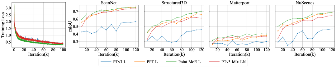
Figure 2: Training Loss and Validation mIoU over time. Left: training loss curves for joint training across multiple domains. Right: validation mIoU on indoor datasets. Point-MoE-L achieves competitive performance to PPT, and both significantly outperform the baseline PTv3-L.

Training efficiency and validation mIoU. Fig. 2 shows the training loss and validation mIoU curves for four models: the baseline PTv3-L, its improved variant PTv3-Mix-LN (which incorporates mixed-domain batches and LayerNorm), PPT-L Wu et al. (2024b), and our proposed Point-MoE-L. All models are trained from scratch across multiple domains. Point-MoE-L converges faster and achieves strong validation mIoU without using explicit dataset labels, matching or exceeding the performance of PPT-L trained with ground-truth domain labels. While all models reach similar training loss, only Point-MoE-L and PPT-L generalize effectively—reinforcing that low training loss is not indicative of strong cross-domain performance. On ScanNet, Structured3D, Matterport3D, and nuScenes, Point-MoE-L shows consistent improvement and avoids early plateaus seen in PPT-L, especially on Structured3D, suggesting stronger long-term learning. PTv3-L fails to generalize and exhibits unstable validation curves. PTv3-Mix-LN improves stability over PTv3-L significantly, but still underperforms Point-MoE-L and PPT-L.

Figure 3: Expert Choices Visualization. Different color represents a different expert. (a) shows a specific expert focusing on edges across the scene, revealing spatially coherent routing. (b) and (c) highlight expert selections in indoor scenes, where semantically related regions (e.g., chair, desk) are consistently routed to the same expert. (d) displays an outdoor scene with sparse LiDAR points, yet the model still demonstrates meaningful routing despite limited geometry.

Expert choice visualization. Fig. 3 showcases expert assignments for a validation scene at selected layers. In (a), we observe that early encoder layers rely heavily on geometric cues for routing. For instance, green experts are consistently activated along object boundaries such as the edges of desks and chairs, while red experts dominate flat surfaces. In (b) and (c), the decoder layers exhibit more semantically meaningful expert selection—likely due to their proximity to the loss function—with distinct experts attending to objects like desks, chairs, floors, and walls. In (d), we examine an outdoor scene with sparse LiDAR data. Despite limited geometric structure, the model still organizes routing meaningfully: nearby points are routed to blue experts, while farther points activate red experts. We include more visualizations in the appendix for completeness. We also note occasional visual artifacts where isolated points are assigned different experts than their neighbors, which may be related to PTv3’s architectural choices such as point serialization or positional encoding.

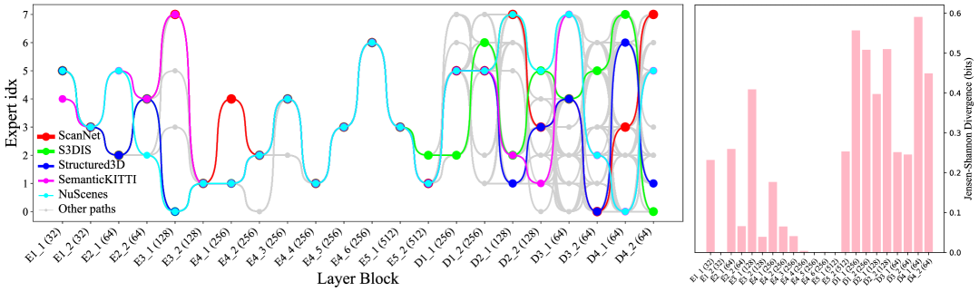
Figure 4: Expert routing behavior across domains. The left panel shows the most frequently used expert paths through each encoder (E-) and decoder (D-) layer, with feature channel sizes marked in parentheses, illustrating the variation in expert selection for tokens from different datasets. The router tends to assign experts based on the input domain, particularly in the decoder MoE layers. To quantify this, we compute the Jensen-Shannon Divergence (JSD) between the expert selection distributions of different datasets at each MoE layer.

Token pathways. To understand how Point-MoE adapts to diverse domains, we analyze expert routing behavior at the token level. Specifically, we track the top-1 expert assignment for each token across all MoE layers and construct full routing trajectories from the final layer back to the first. We then identify the top 100 most frequent expert paths based on their occurrence across all tokens. As shown in Fig. 4, encoder expert paths are substantially less diverse than those in the decoder, indicating that encoder layers perform more domain-agnostic processing. Interestingly, we observe a sparse routing pattern in deeper encoder layers. This may be attributed not to feature reuse, but to the U-Net-style design where features are spatially deep but token sparsity increases, resulting in reduced variability in routing decisions.

When examining domain-level trends, we find that certain dataset pairs—such as SemanticKITTI and nuScenes or ScanNet and Structured3D—share similar expert pathways, suggesting that Point-MoE implicitly clusters domains with related geometric or semantic structures. To quantify these observations, we compute the Jensen-Shannon Divergence (JSD) Lin (1991) between expert selection distributions across datasets at each MoE layer. JSD Lin (1991) is an entropy-based measure of divergence between expert routing distributions across datasets, weighted by their token proportions; its formal definition is provided in the supplementary. As shown in Fig. 4 (right), decoder layers exhibit significantly higher JSD, indicating stronger domain-specific specialization. Several encoder layers also display nontrivial JSD, underscoring the benefit of placing MoE throughout the network.

5 Discussions

This work embraces the “bitter lesson” Sutton (2019) in AI: scalable generalization emerges from flexible architectures trained on diverse data, rather than hand-engineered domain priors Togelius and Yannakakis (2024). We introduce Point-MoE, a mixture-of-experts architecture for 3D understanding that dynamically routes tokens to specialized experts across both indoor and outdoor domains. Our experiments demonstrate that Point-MoE not only achieves competitive performance on seen datasets but, crucially, also generalizes effectively to novel domains without explicit domain labels or supervision. Through careful analysis of expert routing behavior, we show that the model self-organizes around both geometric and semantic structures, adapting its computation pathways to the nature of the input. These results highlight the potential of sparse, modular computation for robust and scalable 3D scene understanding. We provide more analysis of Point-MoE and discuss our limitations in the supplementary material.

6 Acknowledgement

The authors gratefully acknowledge Research Computing at the University of Virginia for providing the computational resources and technical support that made the results in this work possible. Zezhou Cheng acknowledges the Adobe Research Gift, as well as GPU support provided by the Advanced Cyberinfrastructure Coordination Ecosystem: Services & Support (ACCESS) program and the National Artificial Intelligence Research Resource (NAIRR) Pilot program.

Appendix

For a thorough understanding of our Point-MoE, we have compiled a detailed Appendix. The table of contents below offers a quick overview and will guide to specific sections of interest.

section0em1.8em subsection1em2.5em subsubsection2em2.5em

partAppendix

Appendix A Limitations, Licenses and Risks

A.1 Limitations

Our work is limited by computational resource constraints, which restrict the scale of both the Point-MoE architecture and the training datasets. While our results already demonstrate strong generalization across diverse 3D domains, larger models and a broader training corpus could further enhance performance. Additionally, our expert routing relies solely on the standard gating loss without auxiliary regularization for load balancing or diversity, which may lead to suboptimal expert specialization. Finally, the dynamic routing mechanism incurs nontrivial communication and synchronization overhead compared to dense backbones like Point Transformer V3, highlighting the need for more efficient expert parallelism or conditional computation in future work.

A.2 Artifacts and License

We report a list of licenses for all datasets and code used in our experiment in Tab. 4. We strictly follow all the datasets and code licenses and limit the scope of these datasets and code to academic research only.

Table 4: License information for the scientific artifacts used.

Data Sources	URL	License
ScanNet Dai et al. (2017)	Link	ScanNet Terms of Use
Structured3D Zheng et al. (2020)	Link	Structured3D Terms of Use
S3DIS Armeni et al. (2016)	Link	CC BY-NC 4.0
Matterport3D Chang et al. (2017)	Link	Matterport3D License
nuScenes Caesar et al. (2019)	Link	CC BY-NC-SA 4.0
SemanticKITTI Behley et al. (2019a)	Link	CC BY-NC-SA 3.0
Waymo Open Dataset Wang et al. (2019)	Link	Waymo Research License
Software Code	URL	License
Pointcept Contributors (2023)	Link	MIT License

A.3 Ethical concerns and Risks

This study does not involve human subjects or annotators. All experiments are performed on publicly released 3D benchmarks—ScanNet Dai et al. (2017), Structured3D Zheng et al. (2020), S3DIS Armeni et al. (2016), Matterport3D Chang et al. (2017), SemanticKITTI Behley et al. (2019a), nuScenes Caesar et al. (2019), and Waymo Sun et al. (2020)—each distributed under their respective licences. Although these datasets are widely used, they may still reflect geographic, socioeconomic, or sensor–specific biases, which Point-MoE could inherit or amplify when deployed in real-world applications. We therefore encourage future work to develop debiasing techniques, to curate more balanced point-cloud corpora, and to incorporate fairness-oriented evaluation metrics so that cross-domain 3D models can serve all communities responsibly.

Appendix B Additional Experiments

B.1 Experiment Settings

Data. We compare a diverse set of 3D semantic segmentation datasets spanning both indoor and outdoor environments. ScanNet Dai et al. (2017) is a large-scale indoor RGB-D dataset reconstructed from real-world scans of apartments and offices. S3DIS Armeni et al. (2016) contains real indoor scans of commercial buildings, providing richly annotated scenes with diverse architectural structures. Structured3D Zheng et al. (2020) is a synthetic dataset based on photo-realistic rendered scenes from CAD models, offering clean labels and dense annotations. Matterport3D Chang et al. (2017) consists of real RGB-D scans captured in a wide range of residential environments, covering multiple floors and room types.

For outdoor settings, SemanticKITTI Behley et al. (2019a) provides point clouds captured by a 64-beam LiDAR mounted on a car, annotated for semantic understanding of dynamic street scenes. Waymo Open Dataset Wang et al. (2019) extends this setup with more diverse driving environments and higher annotation quality, collected using a custom autonomous vehicle sensor suite. nuScenes Caesar et al. (2019) offers multimodal driving data, including LiDAR scans, captured in urban environments with complex traffic scenarios and longer temporal contexts. We include detailed dataset statistic in Tab. 5.

Furthermore, we provide detailed per-class comparisons on semantic classes for both indoor and outdoor datasets, as shown in Fig. 8 and Fig. 8.

Table 5: Overview of 3D Semantic Segmentation datasets differences. L, W, and H represent the length, width, and height. For all datasets, we use the raw point clouds to obtain the point ranges.

Dataset	Sensor	Point Range (m)	Scene Type
ScanNet Dai et al. (2017)	Reconstructed	L=[-2.13, 17.12], W=[-1.46, 18.19], H=[-0.38, 6.97]	indoor
S3DIS Armeni et al. (2016)	Reconstructed	L=[-37.93, 29.93], W=[-26.08, 46.06], H=[-2.65, 6.58]	indoor
Structured3D Zheng et al. (2020)	Synthetic	L=[-53.70, 52.05], W=[-82.07, 53.43], H=[-0.78, 15.49]	indoor
Matterport3D Chang et al. (2017)	RGB-D Camera	L=[-34.99, 72.17], W=[-57.85, 75.65], H=[-6.79, 10.21]	indoor
SemanticKITTI Behley et al. (2019a)	64-beam LiDAR	L=[-81.15, 80.00], W=[-80.00, 79.99], H=[-32.49, 3.51]	outdoor
Waymo Wang et al. (2019)	64-beam LiDAR	L=[-74.98, 76.53], W=[-75.00, 75.00], H=[-18.36, 6.78]	outdoor
nuScenes Caesar et al. (2019)	32-beam LiDAR	L=[-105.17, 105.25], W=[-105.30, 105.17], H=[-53.42, 20.01]	outdoor

Training. Our default joint training strategy and Point-MoE-L configs are summarized in Tab. 8. We experiment with two batching schemes: (1) single batch, where each iteration samples points exclusively from one dataset, and (2) mix batch, where samples are drawn from multiple datasets with equal probabilities. We find that larger batch sizes lead to more stable expert assignment and better convergence behavior in the Mixture-of-Experts architecture. All models are trained from scratch on the joint multi-domain datasets without any fine-tuning stage.

Table 6: Categorical settings of Indoor Datasets.

Dataset

#C

wall

floor

cabinet

bed

chair

sofa

table

door

window

bookshelf

bookcase

picture

counter

desk

shelves

curtain

dresser

pillow

mirror

ceiling

refrigerator

television

shower curtain

nightstand

toilet

sink

lamp

bathtub

garbagebin

board

beam

column

clutter

otherstructure

otherfurniture

otherprop

other

Structured3D

25

✓

✓

✓

✓

✓

✓

✓

✓

✓

✓

✓

✓

✓

✓

✓

✓

✓

✓

✓

✓

✓

✓

✓

✓

✓

ScanNet

20

✓

✓

✓

✓

✓

✓

✓

✓

✓

✓

✓

✓

✓

✓

✓

✓

✓

✓

✓

✓

S3DIS

13

✓

✓

✓

✓

✓

✓

✓

✓

✓

✓

✓

✓

✓

Matterport3D

21

✓

✓

✓

✓

✓

✓

✓

✓

✓

✓

✓

✓

✓

✓

✓

✓

✓

✓

✓

✓

✓

Table 7: Categorical settings of Outdoor Datasets.

Dataset

#C

car

bicycle

motorcycle

truck

other-vehicle

person

bicyclist

motorcyclist

road

parking

sidewalk

other-ground

building

fence

vegetation

trunk

terrain

pole

traffic-sign

barrier

bus

construction_vehicle

pedestrian

traffic_cone

trailer

driveable_surface

other_flat

manmade

other vehicle

sign

traffic light

construction cone

tree trunk

curb

lane marker

other ground

walkable

SemanticKITTI

19

✓

✓

✓

✓

✓

✓

✓

✓

✓

✓

✓

✓

✓

✓

✓

✓

✓

✓

✓

nuScenes

16

✓

✓

✓

✓

✓

✓

✓

✓

✓

✓

✓

✓

✓

✓

✓

✓

Waymo

22

✓

✓

✓

✓

✓

✓

✓

✓

✓

✓

✓

✓

✓

✓

✓

✓

✓

✓

✓

✓

✓

✓

Table 8: Training settings. H indicates feature dimension.

Joint-training Indoor		Joint-training Indoor-Outdoor		Point-MoE-L
Config	Value	Config	Value	Config	Value
optimizer	AdamW	optimizer	AdamW	# experts	8
scheduler	OneCycleLR	scheduler	OneCycleLR	topk	2
learning rate	0.005	learning rate	0.005	shared expert	0
weight decay	0.05	weight decay	0.05	activation func.	ReLU
batch size	6	batch size	16	auxiliary loss	0
datasets	ScanNet (1), S3DIS (1), Struct.3D (1)	datasets	ScanNet (1), S3DIS (1), Struct.3D (1), nuScenes (1), SemanticKITTI (1)	normalization	BatchNorm
				domain-aware	False
				domain rand.	False
iters	120k	iters	160k	expert capacity	2H

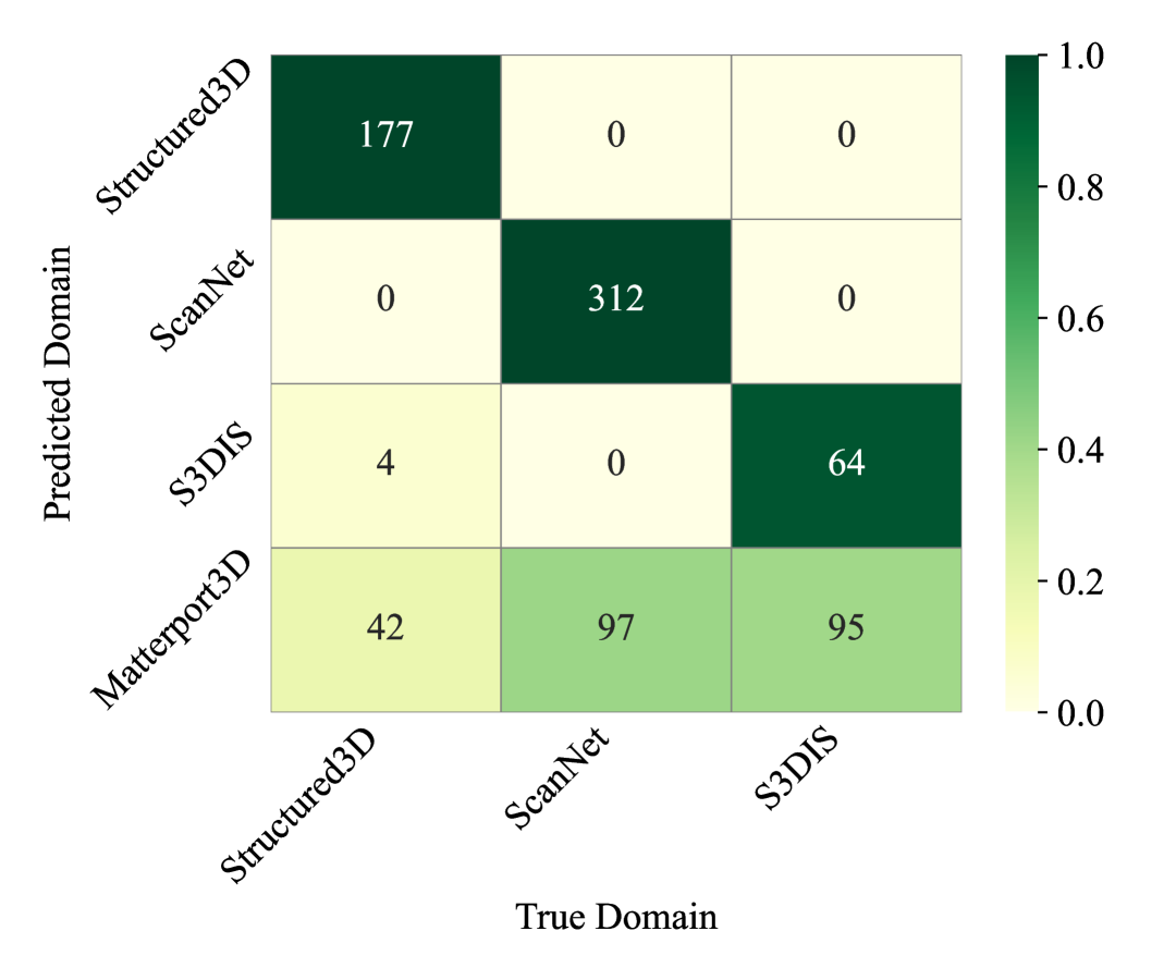
(a) Detector trained on indoor domains

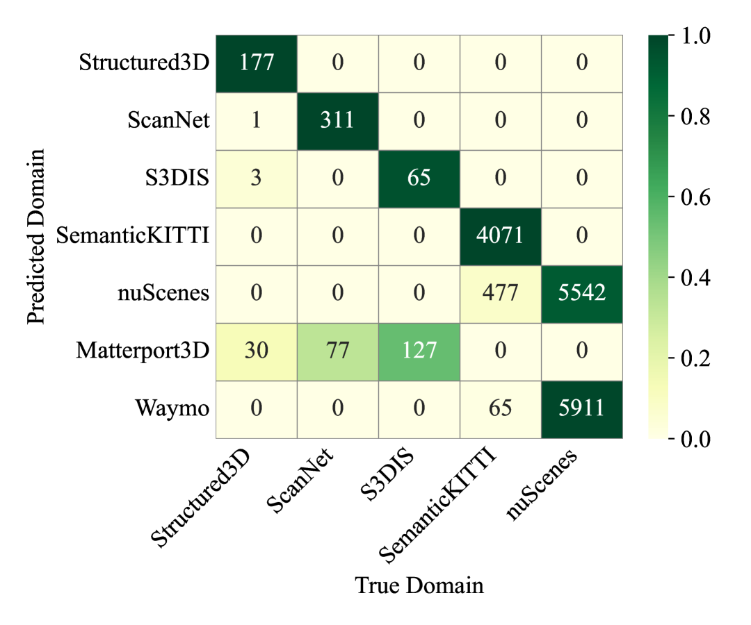
(b) Detector trained on indoor-outdoor domains

Figure 5: Domain Classification Confusion Matrices. (a) Confusion matrix for a domain detector trained only on indoor datasets: Structured3D Zheng et al. (2020), ScanNet Dai et al. (2017), and S3DIS Armeni et al. (2016). (b) Confusion matrix for a detector trained on both indoor and outdoor datasets: Structured3D Zheng et al. (2020), ScanNet Dai et al. (2017), S3DIS Armeni et al. (2016), SemanticKITTI Behley et al. (2019a), and nuScenes Caesar et al. (2019). In both cases, we evaluate generalization to unseen domains. Values are normalized per predicted domain (row-wise).

B.2 Additional Results and Analysis

Domain Detector. To enable domain-aware models at inference time—where ground-truth dataset labels are unavailable—we train a lightweight classifier to predict the domain of an input point cloud. This domain detector serves a purely functional role: it allows domain-conditioned variants of Point-MoE and other baselines to operate in realistic deployment scenarios where users may supply point clouds from unknown or mixed sources. During training, we observe that strong data augmentations (e.g., grid dropout or random cropping) reduce the classifier’s reliability by masking domain-specific cues. To preserve dataset-level characteristics critical for this task, we disable most augmentations and apply only minimal point cropping for efficiency. The domain detector converges quickly, with accuracy stabilizing after just a few epochs. As shown in Fig. 5, it achieves high classification accuracy—99.2% for indoor-only and 95.5% for indoor-outdoor settings—making it suitable for practical use.

The high accuracy of the domain detector suggests that 3D datasets exhibit strong dataset-specific patterns, even when covering similar semantic categories. While we do not perform a detailed analysis of the underlying factors, differences in data acquisition, such as synthetic rendering, RGB-D reconstruction, or LiDAR scanning, are likely to introduce distinct geometric and distributional biases. These biases are implicitly learnable and can be exploited by simple classifiers. For conventional models, such domain discrepancies often necessitate careful data curation or normalization strategies to improve generalization. However, our findings with Point-MoE offer a different perspective: by explicitly modeling distributional variation through expert specialization, the architecture may naturally accommodate such domain shifts without requiring aggressive data homogenization.

Does Point-MoE work on single dataset?

Table 9: Performance of Point-MoE vs. PTv3 on individual datasets. We evaluate both models independently on each dataset to examine whether Point-MoE offers benefits even without cross-domain training. Point-MoE performs comparably to PTv3.

Method	ScanNet	Structured3D	Matterport3D	nuScenes	Waymo	Average
PTv3	75.01	79.37	53.89	77.16	70.20	71.13
Point-MoE	75.63	79.29	53.47	78.24	69.50	71.23

We evaluate Point-MoE without cross-domain supervision by training and testing independently on three indoor datasets (ScanNet Dai et al. (2017), Structured3D Zheng et al. (2020), Matterport3D Chang et al. (2017)) and two outdoor datasets (nuScenes Caesar et al. (2019), Waymo Sun et al. (2020)). On ScanNet and nuScenes, Point-MoE outperforms PTv3 by +0.62 and +1.08, respectively. On Structured3D (evaluated on its test split), performance is nearly identical (–0.08). On Matterport3D (test split) and Waymo (validation split), Point-MoE underperforms PTv3 by –0.42 and –0.70, respectively. On average, Point-MoE achieves 71.23 vs. 71.13 for PTv3 (+0.10). These results suggest that expert specialization can emerge in single-domain settings, but the overall improvement is small and not consistent across datasets. We consider the findings inconclusive.

We hypothesize that Point-MoE may require different configurations or training strategies when applied to a single dataset. In particular, the current gating and load balancing mechanisms are optimized for multi-domain settings, where diverse token distributions benefit from expert diversity. In contrast, single-domain training may benefit from fewer experts, a larger top-$k$, or stronger regularization to avoid expert under-utilization.

Table 10: Joint Training Results on Indoor 3D Semantic Segmentation without Precise Evaluator. Each model is trained jointly on three indoor datasets and evaluated under a domain-agnostic setting without relying on ground-truth domain labels during inference. We report performance when models are required to predict across all domains. To evaluate generalization with a single “generic“ label, results marked (G) use this label for both seen and unseen domains. Unmarked results rely on domain detector predictions..

Methods	Params	Activated	Mix Batch	Layer.	ScanNet	Structured3D	S3DIS	Matterport3D
					Val	Val	Val	Val
Single-dataset training
PTv3-ScanNet Wu et al. (2024a)	46M	46M			74.4	19.4	8.5	37.9
PTv3-Structured3D Wu et al. (2024a)	46M	46M			20.0	78.0	7.0	19.5
PTv3-S3DIS Wu et al. (2024a)	46M	46M			4.9	3.4	66.1	5.2
PTv3-Matterport3D Wu et al. (2024a)	46M	46M			52.7	23.0	9.5	53.6
Domain-agnostic joint training
PTv3-S Wu et al. (2024a)	46M	46M			48.4	57.8	44.1	lightblue27.8
PTv3-S Wu et al. (2024a)	46M	46M	✓		67.7	45.9	62.5	lightblue34.9
PTv3-S Wu et al. (2024a)	46M	46M	✓	✓	70.0	56.0	66.9	lightblue35.6
PTv3-L Wu et al. (2024a)	97M	97M			57.1	58.1	40.3	lightblue31.0
PTv3-L Wu et al. (2024a)	97M	97M	✓		73.3	57.5	67.2	lightblue38.4
PTv3-L Wu et al. (2024a)	97M	97M	✓	✓	70.9	56.5	64.7	lightblue37.2
Point-MoE-S	59M	52M	✓		74.5	66.9	68.6	lightblue40.1
Point-MoE-L	100M	60M	✓		74.3	68.7	68.5	lightblue40.4
Domain-aware joint training
PPT-S Wu et al. (2024b); Wang et al. (2024b)	47M	47M			74.2	58.2	61.0	lightblue24.3
PPT-L Wu et al. (2024b); Wang et al. (2024b)	98M	98M			74.7	64.9	62.0	lightblue27.8
Point-MoE-S	59M	52M	✓		75.6	64.1	63.0	lightblue25.1
Point-MoE-L	100M	60M	✓		74.3	64.9	68.5	lightblue39.5
Point-MoE-G-S	59M	52M	✓		75.3	64.9	60.6	lightblue30.8
Point-MoE-G-S (G)	59M	52M	✓		75.5	65.7	66.7	lightblue39.5
Point-MoE-G-L	100M	60M	✓		75.5	70.0	64.2	lightblue40.2
Point-MoE-G-L (G)	100M	60M	✓		74.7	67.2	65.4	lightblue40.2

Table 11: Cross-Domain 3D Semantic Segmentation on Indoor and Outdoor Scenes without Precise Evaluator. Models are trained jointly on both indoor and outdoor datasets under domain-agnostic supervision and domain-aware joint training settings. (G): Using the “generic“ label during evaluation (see definition above).

Methods	Params	Activated	Mix	Layer.	ScanNet	Structured3D	S3DIS	nuScenes	SemKITTI	Matterport3D	Waymo
					Val	Val	Val	Val	Val	Val	Val
Domain-agnostic joint training
PTv3-L Wu et al. (2024a)	97M	97M			55.9	47.6	19.3	42.9	35.3	lightblue31.8	lightblue12.4
PTv3-L Wu et al. (2024a)	97M	97M	✓		73.4	61.9	61.4	64.7	59.3	lightblue38.9	lightblue22.8
PTv3-L Wu et al. (2024a)	97M	97M	✓	✓	73.6	61.3	65.1	64.5	59.7	lightblue37.1	lightblue21.9
Point-MoE-L	100M	60M	✓		74.8	70.1	65.7	68.7	60.4	lightblue40.3	lightblue23.4
Domain-aware joint training
PPT-L Wu et al. (2024b); Wang et al. (2024b)	98M	98M			75.2	67.5	61.0	57.2	64.0	lightblue20.8	lightblue16.0
Point-MoE-L	100M	60M	✓		75.2	67.0	61.8	59.6	62.1	lightblue19.1	lightblue17.9
Point-MoE-G-L	100M	60M	✓		75.8	69.3	62.7	67.6	61.1	lightblue22.8	lightblue23.2
Point-MoE-G-L (G)	100M	60M	✓		75.5	71.6	68.0	68.3	60.8	lightblue37.4	lightblue23.4

Table 12: Joint Training Performance on Indoor 3D Semantic Segmentation with Ground-Truth Domain Labels. We additionally evaluate models trained on indoor datasets using domain-aware supervision, where explicit ground-truth domain labels are provided during training to guide the learning process.

Methods	Params	Activated	Mix Batch	ScanNet	Structured3D		S3DIS
				Val	Val	Test	Val
Domain-aware joint training with G.T. labels
PPT-S Wu et al. (2024b); Wang et al. (2024b)	47M	47M		74.7	60.9	65.5	71.6
PPT-L Wu et al. (2024b); Wang et al. (2024b)	98M	98M		74.6	60.9	62.6	69.2
Point-MoE-S	59M	52M	✓	76.7	66.7	72.3	71.9
Point-MoE-L	100M	60M	✓	75.6	69.7	71.3	69.6
Point-MoE-G-S	59M	52M	✓	75.7	69.1	70.8	68.1
Point-MoE-G-L	100M	60M	✓	76.7	68.1	69.6	67.1

Table 13: Joint Training Performance on Indoor-Outdoor 3D Semantic Segmentation with Ground-Truth Domain Labels. We evaluate models trained on indoor-outdoor datasets using domain-aware supervision with ground truth labels.

Methods	Params	Activated	Mix	ScanNet	Structured3D		S3DIS	nuScenes	SemKITTI
				Val	Val	Test	Val	Val	Val
Domain-aware joint training with G.T. labels
PPT-L Wu et al. (2024b); Wang et al. (2024b)	98M	98M		76.7	67.2	66.0	71.2	72.6	66.9
Point-MoE-L	100M	60M	✓	76.8	69.6	70.1	70.6	72.4	64.5
Point-MoE-G-L	100M	60M	✓	77.0	74.9	73.2	71.6	73.0	64.3

B.3 Additional Main Results

Results without precise evaluator. The results reported in Tab. 1 and Tab. 2 are obtained using the precise evaluator provided by Pointcept Contributors (2023). The precise evaluator first splits each scene into multiple overlapping chunks, then performs model inference on each chunk individually. After inference, it aggregates predictions across chunks through a voting mechanism to refine the final output. We typically observe a gain of 2–4% in accuracy on each dataset using this method. While effective, the precise evaluator introduces additional runtime overhead during evaluation. Moreover, we note that this form of ensembling may hurt overall performance when the model’s predictions are unreliable in early chunks, as incorrect outputs are also accumulated in the final vote. To support convenient and reproducible benchmarking for the community, we include results with the precise evaluator in the main text and provide additional baseline results without it elsewhere in the paper.

From both Tab. 1 and Tab. 2, we observe that Point-MoE outperforms the baselines in most domains in both the indoor-only and indoor-outdoor joint training settings. These results are consistent with those obtained using the precise evaluator reported in the main text. We do not observe any contradictory trends, as the precise evaluator typically improves all methods by a similar margin of 2–4%. As such, our analysis and conclusions align closely with those presented in the main text. How Strong is Domain-Aware Point-MoE? In the main text, we compare domain-agnostic and domain-aware settings and observe that domain-aware Point-MoE does not consistently outperform its domain-agnostic counterpart. Here we want to offer discussions and analysis to explain the reason. One contributing factor is the reliance on the domain predictor as we detailed in sec. B.2. Although the domain predictor achieves high classification accuracy, even minor errors can lead to noticeable performance degradation—either by misrouting inputs to suboptimal experts in Point-MoE or by selecting incorrect normalization statistics in PPT. To better isolate this effect, we include results in Tab. 12 and Tab. 13, where we evaluate domain-aware Point-MoE using ground-truth domain labels.

In general, Point-MoE continues to outperform standard baselines in both settings. Moreover, we find that domain-aware Point-MoE with access to ground-truth labels achieves better performance on seen domains, while domain-agnostic Point-MoE trained with domain-randomized data generalizes better to unseen domains. Interestingly, we also observe that Point-MoE trained with generic (i.e., domain-agnostic) supervision performs well even on seen domains when exposed to more diverse training inputs. This suggests that domain-randomization during training may benefit performance across both seen and unseen domains in challenging settings. Finally, we note that domain-aware Point-MoE can yield stronger results when accurate domain labels are available at inference time.

Appendix C Additional Visualization and Discussions on Point-MoE

C.1 t-SNE

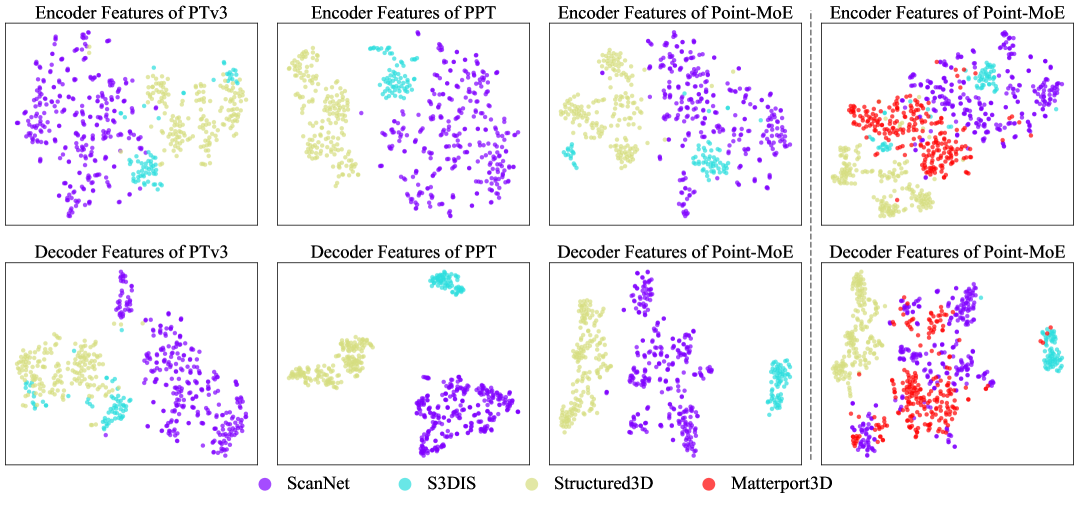
Figure 6: t-SNE Visualization. The first three columns illustrate feature similarities and differences across PTv3, PPT, and Point-MoE for both encoder and decoder layers. The rightmost column highlights how Point-MoE generalizes to unseen domains, with Matterport3D features aligning closely with the most relevant seen domains—demonstrating robust cross-domain generalization.

Fig. 6 presents t-SNE visualizations van der Maaten and Hinton (2008) of encoder and decoder features from PTv3, PPT Wu et al. (2024b), and Point-MoE. PTv3 exhibits no clear separation in either encoder or decoder spaces, indicating its inability to structure domain-specific representations. In contrast, PPT shows strongly separated clusters for each domain at both encoder and decoder levels, suggesting it overfits to domain-specific patterns. While this benefits seen domains, it may hinder generalization to unseen settings.

Point-MoE, however, reveals a more interesting behavior. Its encoder features remain entangled across domains—indicating shared representation learning—while its decoder learns to disentangle domain-specific structures. This division of labor suggests that Point-MoE effectively performs domain inference within the model, without requiring explicit domain labels. Most notably, in the unseen Matterport3D domain, Point-MoE maps samples to nearby clusters of the most relevant seen domains (e.g., ScanNet), enabling strong generalization. This implicit alignment underscores the model’s ability to organize and interpret new environments by leveraging expertise learned from diverse sources.

C.2 Semantic Concept Distribution over Experts

Expert Specialization Word Cloud. To visualize expert specialization, we collect the semantic predictions from each expert in the decoder layers of Point-MoE. During inference, we log which expert is selected for each point and record the corresponding semantic prediction. For each expert, we compute the frequency distribution of predicted classes across the entire validation set and display the most frequent class as a word cloud. Colors indicate the originating dataset of the prediction (e.g., ScanNet, S3DIS, etc.), providing insight into cross-domain consistency.

We observe several interesting patterns in the expert specialization behavior. (1) In each decoder layer, there is typically at least one expert with a strong preference for outdoor data. For example, Decoder 0_0 Expert 7, Decoder 1_1 Expert 1, and Decoder 2_1 Expert 2 predominantly handle outdoor scenes. (2) Generic or ambiguous semantic classes such as otherfurniture or other-ground never dominate the assignment of any expert, suggesting that these classes are more diffusely distributed and do not concentrate through the routing mechanism.

From the visualization in Fig. 7, we observe several notable trends. Specialization emerges clearly: within each decoder block, experts tend to focus on semantically coherent regions such as bed, bathtub, window, or trailer, suggesting that experts develop functional roles under shared supervision. In many blocks, multiple experts cover similar classes, yet differ in dataset association, indicating potential cross-domain generalization. For instance, certain experts across blocks frequently predict bed or toilet across multiple indoor datasets, hinting at robust feature preferences. We also observe signs of dataset sensitivity. Classes like trailer, parking, and terrain appear predominantly in SemanticKITTI and nuScenes, while sink, shower curtain, and dresser are more common in Structured3D. Comparing across decoder layers, earlier blocks display a broader mix of classes per expert, while deeper blocks exhibit more focused and object-specific specialization, reflecting an increasing semantic refinement through the decoding process.

These findings suggest that Point-MoE encourages structured representation learning, where each expert in a given layer implicitly captures recurring semantic or geometric patterns, even without explicit specialization objectives or layer-to-layer consistency.

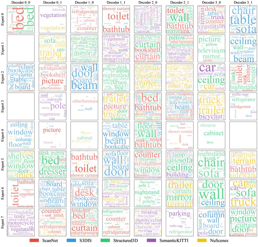
Figure 7: Expert Specialization Word Cloud. All classes’ frequencies of selecting their top-1 expert are measured on the validation set. Colors indicate the originating dataset of the class (e.g., ScanNet, S3DIS, etc.), providing insight into cross-domain consistency.

Expert Probability Stack Visualization. To complement the word cloud analysis, we provide fine-grained views of expert behavior in Fig. 8, Fig. 9, Fig. 10 and Fig. 11. For each semantic class, we visualize the soft routing probabilities across all experts within a specific decoder block. Each horizontal bar corresponds to a class, segmented proportionally by the probability of top-1 expert assignment to each expert. This representation allows us to examine how responsibilities are distributed across experts for different categories.

We observe that certain semantic classes are strongly associated with a small number of experts. For example, bed, bathtub, and toilet are consistently routed to a narrow subset of experts, reflecting high specialization. In contrast, classes such as wall and vegetation are distributed across multiple experts, likely due to their spatial extent and ubiquity in scenes. Some experts show broad activation across diverse classes, while others are more selective, indicating a balance between general-purpose and task-specific routing. Several consistent patterns emerge in the decoder. In Decoder Layer 3 Block 0, both truck and trailer are primarily assigned to Expert 3, suggesting structural similarity. In Decoder Layer 3 Block 1, dresser, nightstand, and counter are all routed to Expert 2, reflecting shared visual or functional features. In Decoder Layer 0 Block 1, traffic cone and barrier exhibit nearly identical routing distributions, likely due to their geometric similarity and outdoor context. These observations confirm that the model learns structured yet flexible routing strategies, shaped by both semantic identity and spatial context.

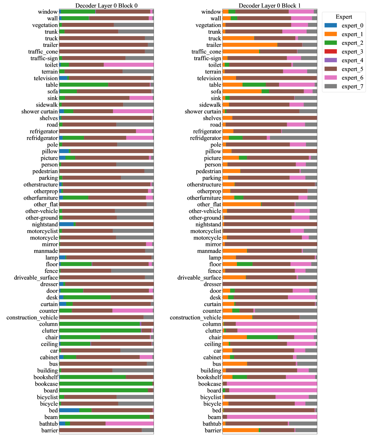
Figure 8: Expert Choices Visualization for Decoder Layer 0.

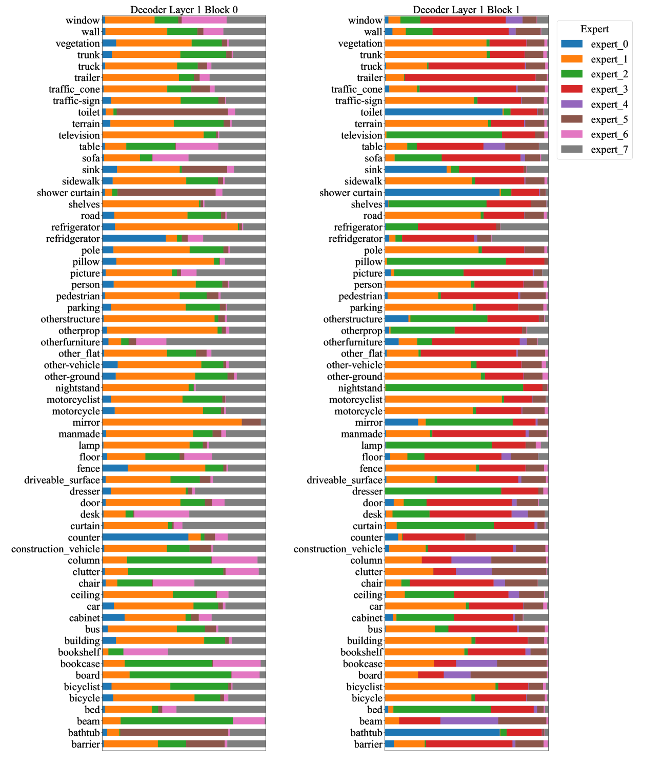
Figure 9: Expert Choices Visualization for Decoder Layer 1.

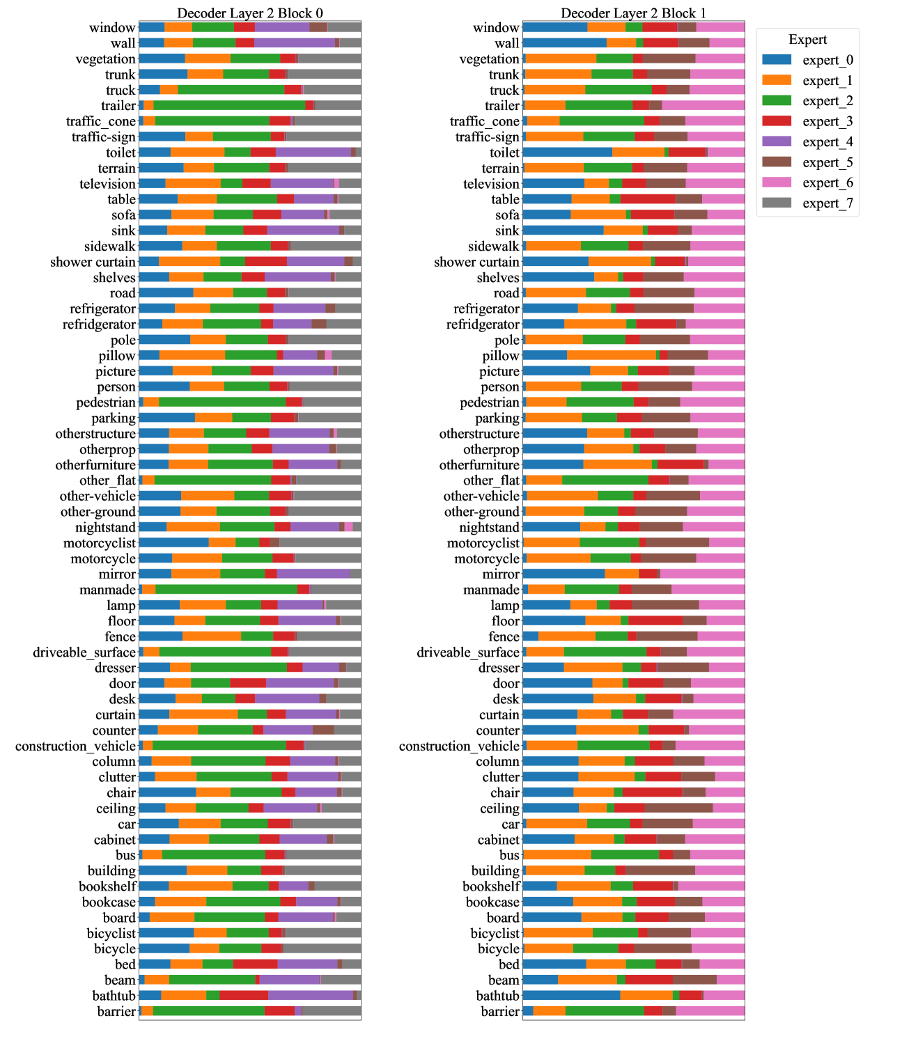
Figure 10: Expert Choices Visualization for Decoder Layer 2.

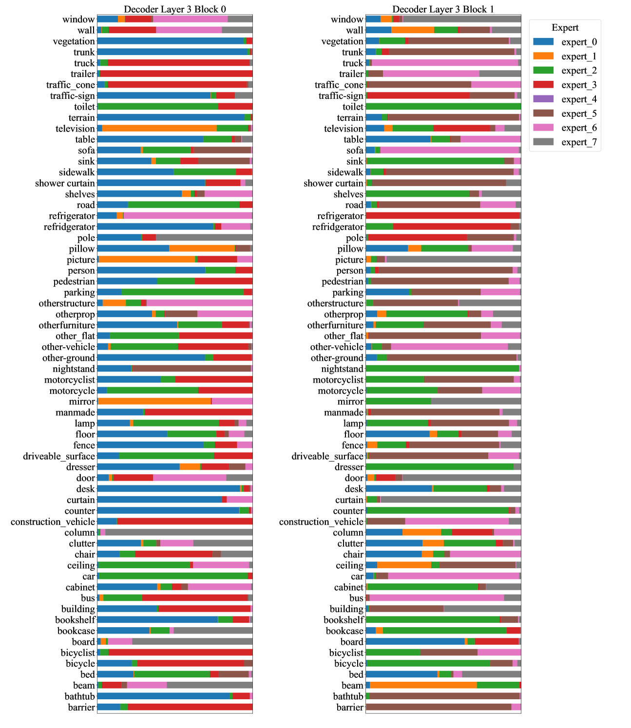
Figure 11: Expert Choices Visualization for Decoder Layer 3.

C.3 Expert Evolution.

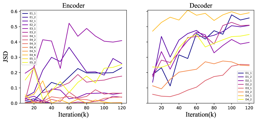
Figure 12: JSD Dynamics During Training. We visualize the Jensen-Shannon Divergence (JSD) between expert assignment distributions across datasets to study how expert specialization emerges over time. The plots illustrate JSD dynamics across training iterations for both encoder and decoder layers.

In Fig. 12, we track the Jensen-Shannon Divergence (JSD) between expert assignment distributions across different datasets every 10k training iterations to analyze how expert specialization evolves over time. Let $P_{1},P_{2},\dots,P_{n}$ denote the expert routing distributions for each of the $n$ datasets, where each $P_{i}$ is a categorical distribution over experts. Specifically, let $P_{i}(e)$ denote the fraction of tokens from dataset $i$ that are routed to expert $e$. Let $\pi_{1},\pi_{2},\dots,\pi_{n}$ be the corresponding weights assigned to each dataset, satisfying $\sum_{i=1}^{n}\pi_{i}=1$. These weights reflect the proportion of tokens contributed by each dataset. The Jensen-Shannon Divergence is defined as:

$$\text{JSD}_{\pi}(P_{1},P_{2},\dots,P_{n})=H\mathopen{}\mathclose{{\left(\sum_{i=1}^{n}\pi_{i}P_{i}}}\right)-\sum_{i=1}^{n}\pi_{i}H(P_{i}),$$

where $H(P)=-\sum_{x}P(x)\log P(x)$ denotes the Shannon entropy. This formulation captures the degree of divergence between datasets in terms of how they utilize the experts, providing a measure of specialization and separation over time.

In the early stages (10k–30k), JSD values remain low across most experts, indicating that the routing behavior is largely uniform across datasets and experts have not yet developed distinct roles. Between 40k and 60k iterations, we begin to observe divergence among certain experts, marking the onset of specialization. This trend continues and becomes more pronounced by 80k iterations, where several experts display increasingly distinct assignment distributions. By 100k iterations, the JSD curves stabilize, suggesting that expert roles have converged. Some experts diverge earlier and more sharply, indicating faster specialization, while others evolve more gradually. Overall, this analysis confirms that expert diversity in Point-MoE is not predefined but emerges progressively through training.

In the encoder, we observe that some experts maintain JSD values close to zero throughout training, suggesting that their routing behavior remains largely random and undifferentiated. This observation aligns with Fig. 4, where certain encoder experts do not exhibit clear dataset- or task-specific specialization. This raises the possibility that not all encoder layers require MoE modules, or that additional regularization or training signals may be needed to encourage expert differentiation in the encoder. Nonetheless, we do observe that some encoder experts do specialize over time, indicating that meaningful expert roles can still emerge under the right conditions.

In the decoder, we observe that all experts exhibit high JSD values, indicating that their routing behavior becomes highly specialized and dataset-dependent. Additional visualizations of expert assignments can be found in Sec. C.4, further illustrating this specialization.

C.4 More Expert Choice Visualization

Fig. 13, Fig. 14, Fig. 15, Fig. 16, Fig. 17, Fig. 18, and Fig. 19 showcase expert assignments for a validation scene across all layers. Due to the hierarchical structure of the PTv3 backbone, we observe denser point cloud representations at the input and output stages, with sparser intermediate features. This design leads to visibly varying point densities and detail levels across the network. We also observe block-like artifacts in some visualizations, which are likely attributed to PTv3’s point serialization strategy. In the encoder, certain experts occasionally exhibit collapsed or spatially clustered behavior—a phenomenon we refer to as “expert clasping.” A deeper investigation into this behavior is left for future work. In the decoder layers, expert assignments closely resemble semantic segmentation outputs, even though the visualizations reflect only expert routing decisions rather than predicted labels. This suggests that experts naturally specialize in semantically coherent regions, despite the absence of explicit supervision guiding their roles.

In Fig. 13, we observe that early encoder layers primarily rely on geometric cues for expert routing. For example, certain experts—such as the green one—are consistently activated along object boundaries, including the edges of desks and chairs, while others tend to dominate on flat or horizontal surfaces. In the decoder layers, expert assignments become more semantically meaningful, with different experts focusing on specific object categories such as desks, chairs, walls, and floors.

In Fig. 14, we observe a similar overall pattern to ScanNet Dai et al. (2017). In the encoder, expert assignments are primarily driven by local geometric structure, with clear attention to furniture boundaries and wall intersections. Notably, edge-aware routing persists deeper into the encoder—for example, in encoder layer 2 block 0, certain experts remain focused on object contours. In the decoder, expert activation becomes increasingly aligned with semantic regions, such as tables, chairs, and structural elements. Despite the architectural and layout differences from ScanNet, the expert routing in S3DIS remains semantically consistent across the scene.

Fig. 15 illustrates expert routing on Structured3D Zheng et al. (2020), a synthetic dataset. Compared to real-world datasets, the expert assignment patterns appear sharper and more consistent, likely due to the absence of sensor noise and reconstruction artifacts. Some experts are clearly focused on flat regions, such as beds or floor. In the decoder layers, expert specialization aligns closely with object instances, and the separation across semantic regions is more distinct and well-defined, highlighting the benefits of clean, synthetic geometry for expert differentiation.

Fig. 16 presents expert routing on Matterport3D Chang et al. (2017), which contains complex residential environments. In the early encoder layers, we observe clear expert usage patterns—for instance, a distinct separation between vertical and horizontal surfaces. In the decoder layers, expert assignments become more semantically meaningful, with experts specializing in large structural elements such as floors and ceilings, as well as common household objects like counters, sofas, and chairs. Notably, Matterport3D is not included in the training set, so this behavior reflects Point-MoE’s ability to generalize expert specialization to unseen domains.

In Fig. 17, we examine an outdoor scene from SemanticKITTI Behley et al. (2019a), characterized by sparse LiDAR data. Despite the limited geometric density, the model still exhibits meaningful expert routing: nearby points tend to be assigned to certain experts, while distant points activate others. Although the transition from geometry-driven to semantically informed expert assignment remains observable, it appears noisier due to the inherent sparsity and irregularity of the input point cloud.

Fig. 18 shows expert routing on nuScenes Caesar et al. (2019), an outdoor dataset with lower-resolution LiDAR data. In the encoder layers, expert assignments appear more fragmented, likely due to the reduced point density. Nonetheless, we observe that closer points are often routed to specific experts, while distant points are handled by others, indicating a spatially aware routing pattern. In the decoder layers, expert assignments become more semantically coherent, with specialization emerging for vehicle bodies, building facades, and road surfaces based on point position and distance.

Fig. 19 presents expert routing on Waymo Sun et al. (2020), an unseen dataset characterized by 64-beam LiDAR scans. In the encoder, experts exhibit structured activation patterns even in early layers, with clear delineation between flat surfaces and protruding objects. In the decoder layers, expert routing becomes more semantically aligned, with experts consistently activated over road surfaces, vehicle bodies, and trees. The assigned regions remain compact and well-separated.

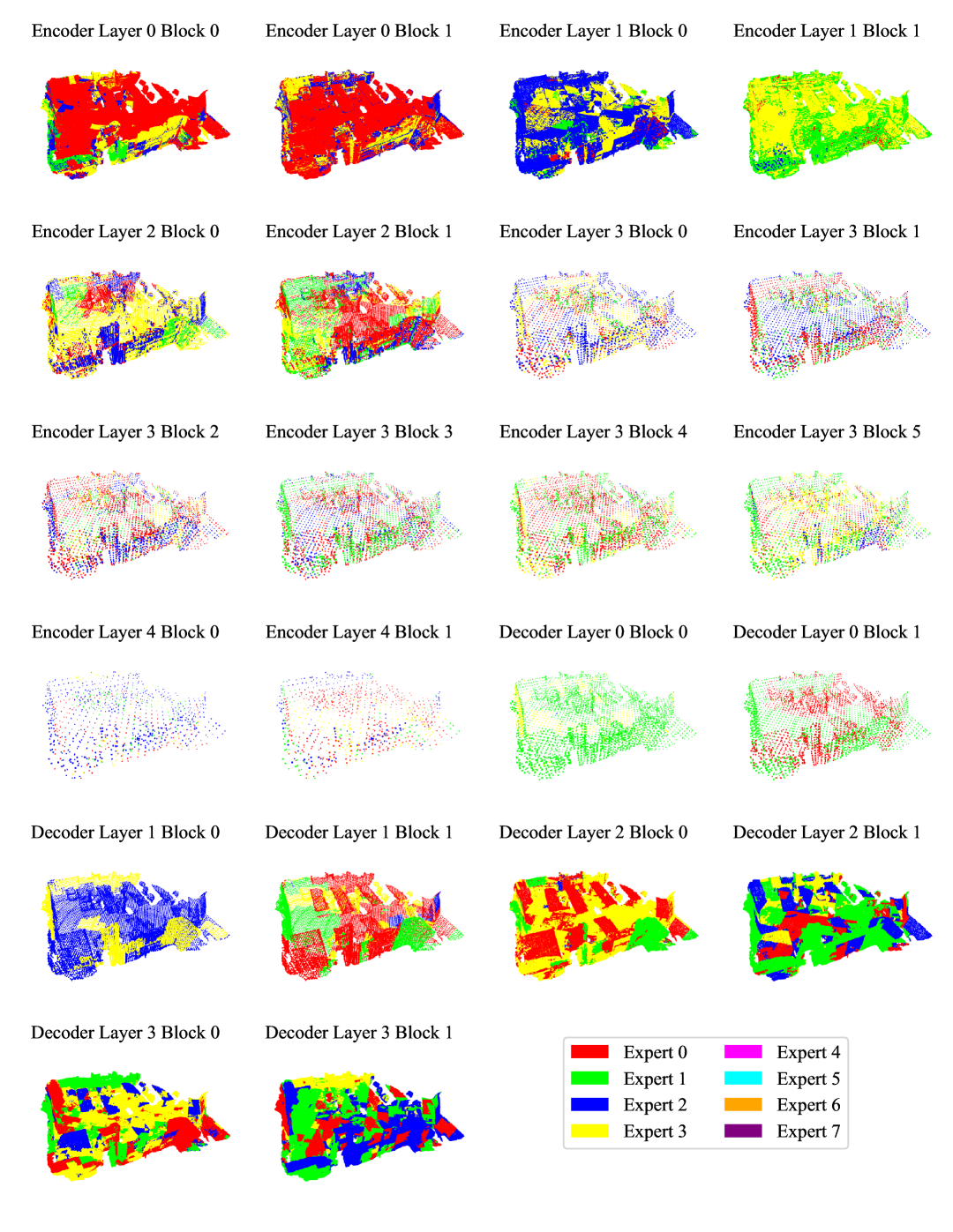
Figure 13: Point-MoE’s Expert Choice Visualization on ScanNet. Each point is colored by its assigned expert across encoder and decoder blocks. Early layers show structured expert usage, while deeper layers exhibit more mixed routing, reflecting the evolving representation dynamics throughout the network.

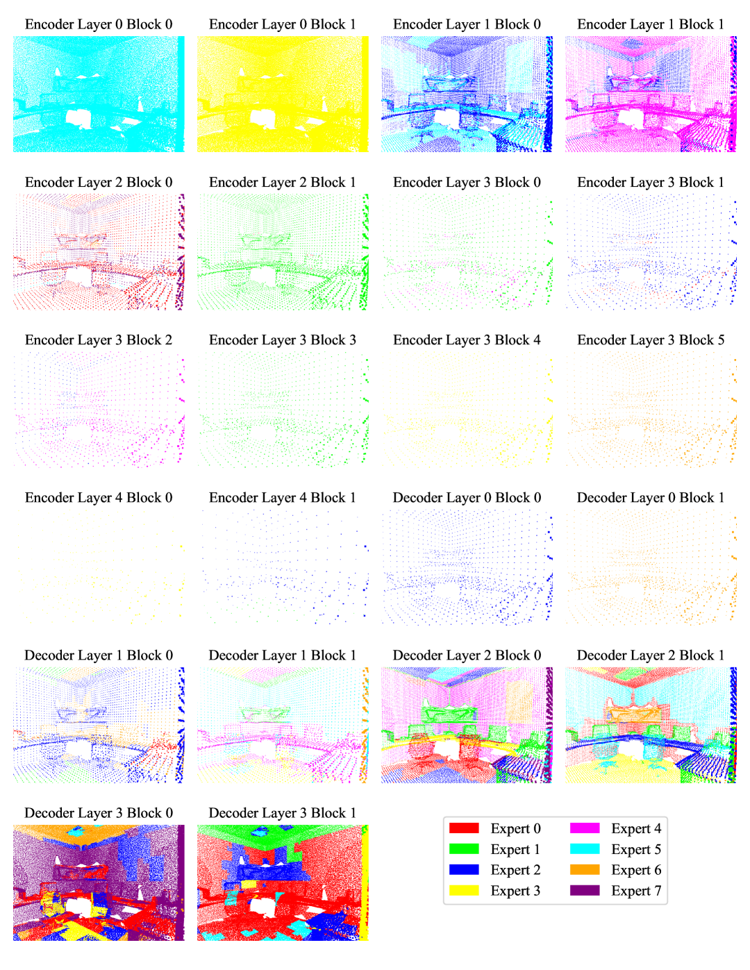
Figure 14: Point-MoE’s Expert Choice Visualization on S3DIS. Each point is color-coded based on the expert it was routed to across both encoder and decoder blocks. The earlier layers demonstrate clear structure in expert assignments, whereas the later layers reveal more diverse routing patterns, indicating evolving feature representations.

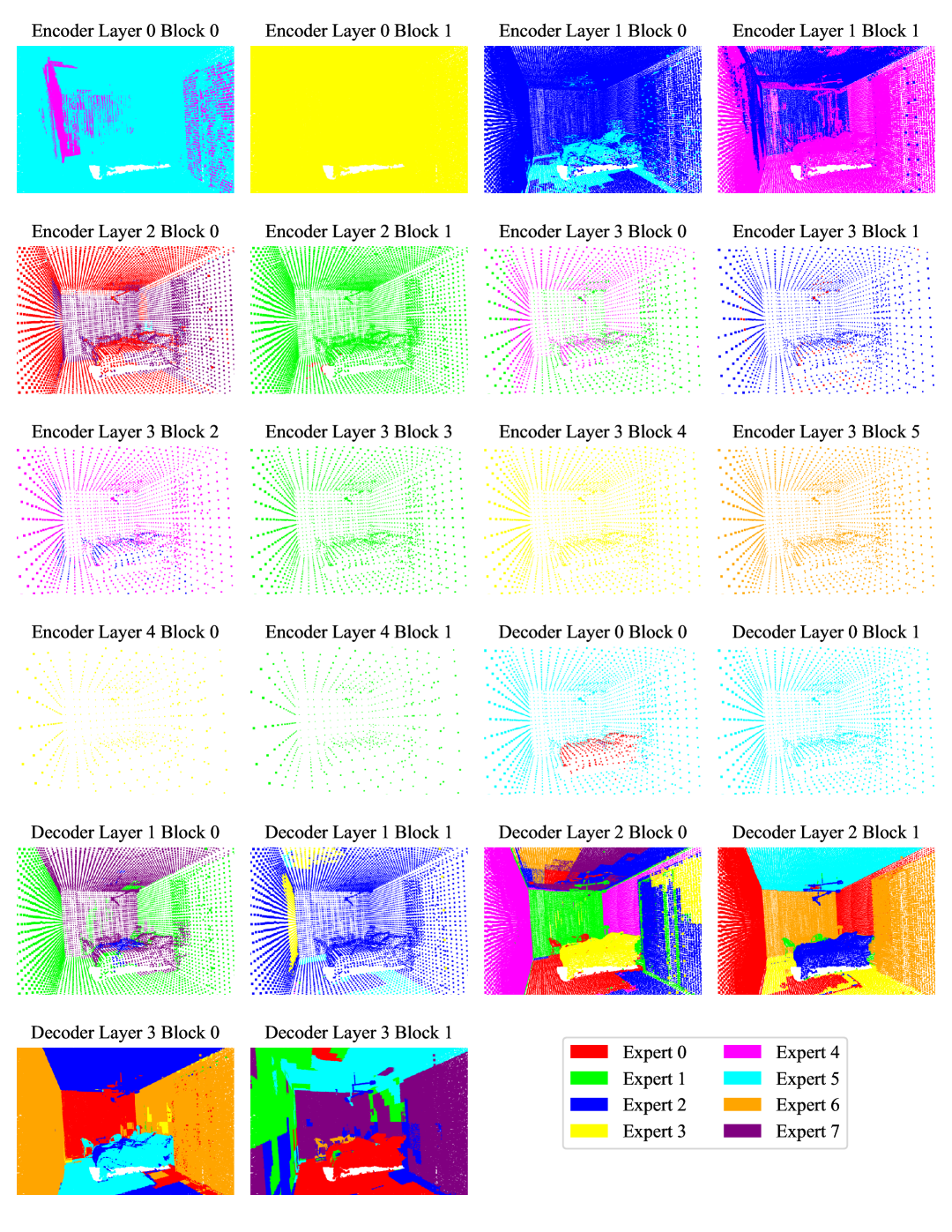
Figure 15: Point-MoE’s Expert Choice Visualization on Structured3D. Points are colored by their designated experts in the encoder and decoder. While the initial layers display consistent expert allocation, the deeper layers show a blend of routing decisions, highlighting the network’s shifting representational strategy.

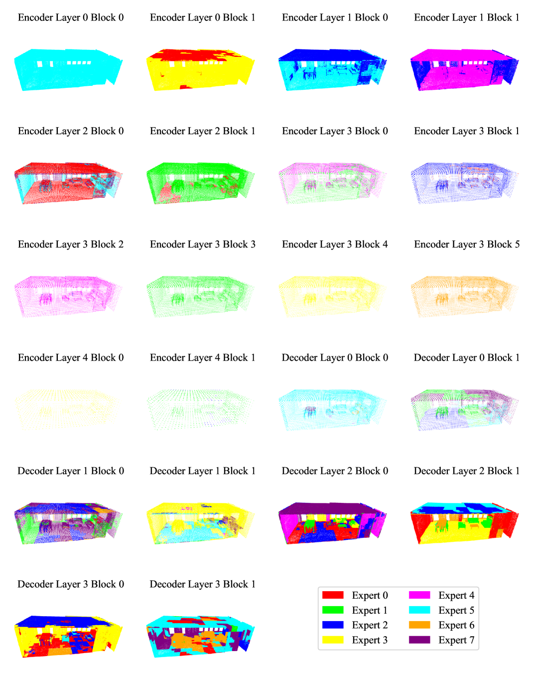
Figure 16: Point-MoE’s Expert Choice Visualization on Matterport3D. Color represents the expert assigned to each point throughout the encoder and decoder. Structured expert usage is visible in early stages, transitioning to more varied routing in deeper layers, signaling changes in how features are processed.

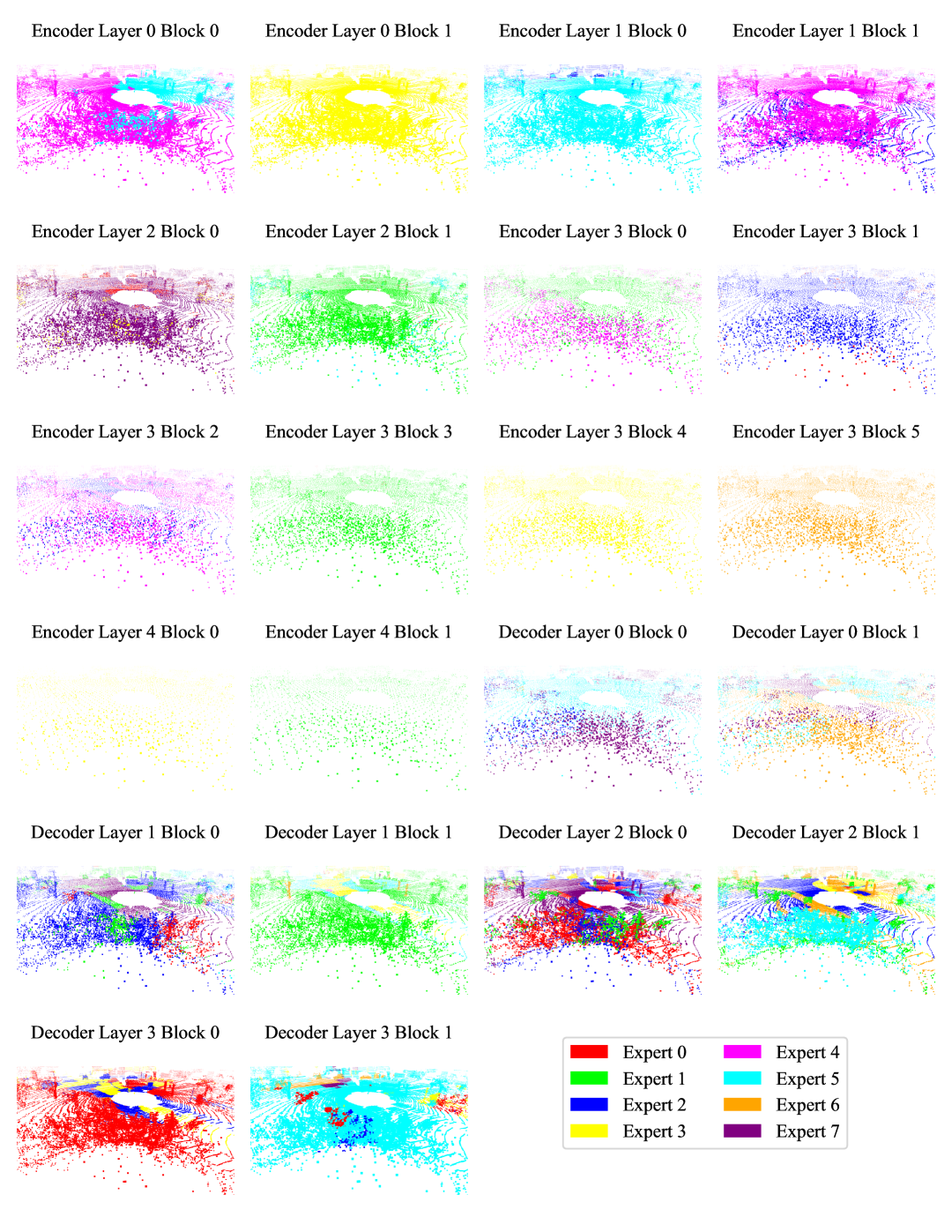
Figure 17: Point-MoE’s Expert Choice Visualization on SemanticKITTI. The expert responsible for each point, shown through color, spans the encoder and decoder blocks. Initially, expert usage is highly organized, but becomes more dispersed in later layers, capturing the transformation in representation over depth.

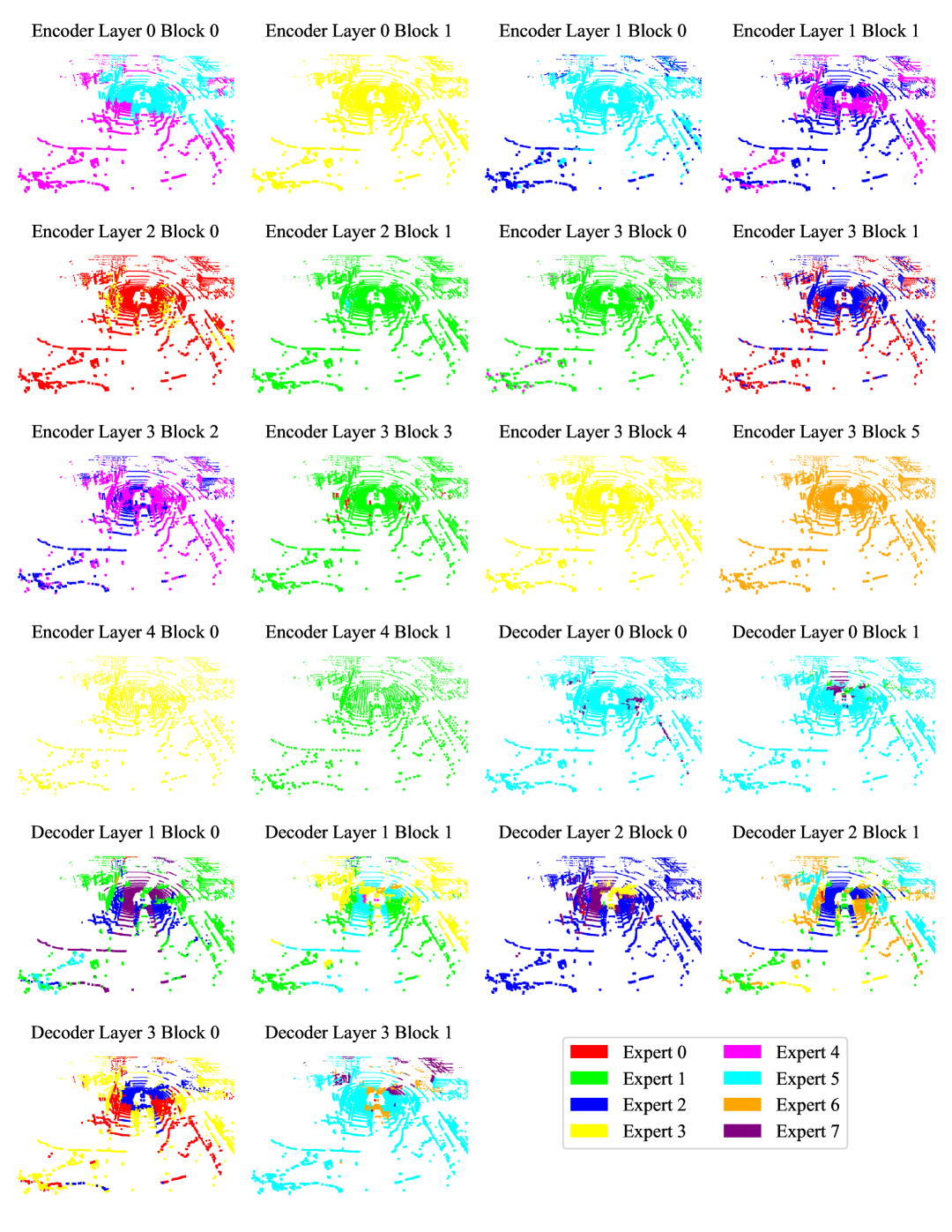
Figure 18: Point-MoE’s Expert Choice Visualization on NuScene. Each point is colored according to its corresponding expert across the network’s layers. Early encoder and decoder blocks exhibit distinct expert patterns, while deeper layers demonstrate a more distributed and dynamic routing behavior.

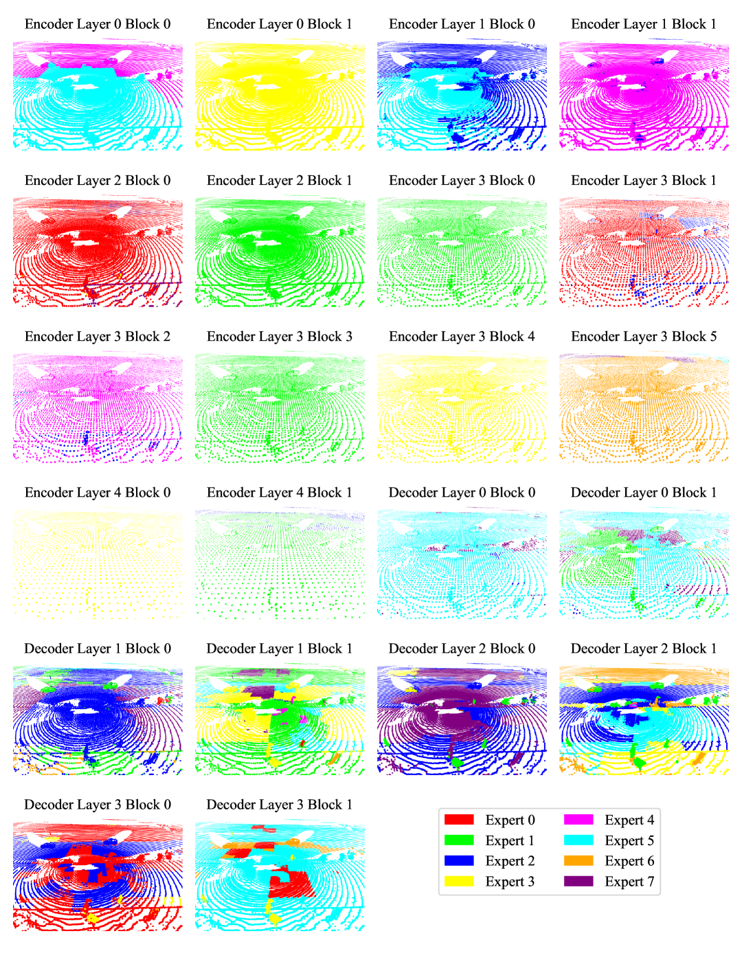
Figure 19: Point-MoE’s Expert Choice Visualization on Waymo. Color indicates the expert each point is assigned to across encoder and decoder stages. Early network layers maintain structured expert routes, but this structure relaxes in deeper layers, illustrating evolving internal representations.

References

- Agarap (2019) Abien Fred Agarap. 2019. Deep learning using rectified linear units (relu).
- Armeni et al. (2016) Iro Armeni, Ozan Sener, Amir R. Zamir, Helen Jiang, Ioannis Brilakis, Martin Fischer, and Silvio Savarese. 2016. 3d semantic parsing of large-scale indoor spaces. In 2016 IEEE Conference on Computer Vision and Pattern Recognition (CVPR), pages 1534–1543.
- Avetisyan et al. (2024) Armen Avetisyan, Christopher Xie, Henry Howard-Jenkins, Tsun-Yi Yang, Samir Aroudj, Suvam Patra, Fuyang Zhang, Duncan Frost, Luke Holland, Campbell Orme, Jakob Engel, Edward Miller, Richard Newcombe, and Vasileios Balntas. 2024. Scenescript: Reconstructing scenes with an autoregressive structured language model.
- Ba et al. (2016) Jimmy Lei Ba, Jamie Ryan Kiros, and Geoffrey E. Hinton. 2016. Layer normalization.
- Bain et al. (2021) Max Bain, Arsha Nagrani, Gül Varol, and Andrew Zisserman. 2021. Frozen in time: A joint video and image encoder for end-to-end retrieval. In IEEE International Conference on Computer Vision.
- Behley et al. (2019a) J. Behley, M. Garbade, A. Milioto, J. Quenzel, S. Behnke, C. Stachniss, and J. Gall. 2019a. SemanticKITTI: A Dataset for Semantic Scene Understanding of LiDAR Sequences. In Proc. of the IEEE/CVF International Conf. on Computer Vision (ICCV).
- Behley et al. (2019b) J. Behley, M. Garbade, A. Milioto, J. Quenzel, S. Behnke, C. Stachniss, and J. Gall. 2019b. SemanticKITTI: A Dataset for Semantic Scene Understanding of LiDAR Sequences. In Proc. of the IEEE/CVF International Conf. on Computer Vision (ICCV).
- Brown et al. (2020) Tom B. Brown, Benjamin Mann, Nick Ryder, Melanie Subbiah, Jared Kaplan, Prafulla Dhariwal, Arvind Neelakantan, Pranav Shyam, Girish Sastry, Amanda Askell, Sandhini Agarwal, Ariel Herbert-Voss, Gretchen Krueger, Tom Henighan, Rewon Child, Aditya Ramesh, Daniel M. Ziegler, Jeffrey Wu, Clemens Winter, Christopher Hesse, Mark Chen, Eric Sigler, Mateusz Litwin, Scott Gray, Benjamin Chess, Jack Clark, Christopher Berner, Sam McCandlish, Alec Radford, Ilya Sutskever, and Dario Amodei. 2020. Language models are few-shot learners.
- Byeon et al. (2022) Minwoo Byeon, Beomhee Park, Haecheon Kim, Sungjun Lee, Woonhyuk Baek, and Saehoon Kim. 2022. Coyo-700m: Image-text pair dataset. https://github.com/kakaobrain/coyo-dataset.
- Caesar et al. (2019) Holger Caesar, Varun Bankiti, Alex H. Lang, Sourabh Vora, Venice Erin Liong, Qiang Xu, Anush Krishnan, Yu Pan, Giancarlo Baldan, and Oscar Beijbom. 2019. nuscenes: A multimodal dataset for autonomous driving. arXiv preprint arXiv:1903.11027.
- Caesar et al. (2020) Holger Caesar, Varun Bankiti, Alex H. Lang, Sourabh Vora, Venice Erin Liong, Qiang Xu, Anush Krishnan, Yu Pan, Giancarlo Baldan, and Oscar Beijbom. 2020. nuscenes: A multimodal dataset for autonomous driving.
- Chang et al. (2017) Angel Chang, Angela Dai, Thomas Funkhouser, Maciej Halber, Matthias Nießner, Manolis Savva, Shuran Song, Andy Zeng, and Yinda Zhang. 2017. Matterport3d: Learning from rgb-d data in indoor environments.
- Chen et al. (2023) Shizhe Chen, Ricardo Garcia, Cordelia Schmid, and Ivan Laptev. 2023. Polarnet: 3d point clouds for language-guided robotic manipulation.
- Chen et al. (2020) Siheng Chen, Baoan Liu, Chen Feng, Carlos Vallespi-Gonzalez, and Carl Wellington. 2020. 3d point cloud processing and learning for autonomous driving.
- Chen et al. (2017) Xiaozhi Chen, Huimin Ma, Ji Wan, Bo Li, and Tian Xia. 2017. Multi-view 3d object detection network for autonomous driving.
- Chen et al. (2022) Zitian Chen, Yikang Shen, Mingyu Ding, Zhenfang Chen, Hengshuang Zhao, Erik Learned-Miller, and Chuang Gan. 2022. Mod-squad: Designing mixture of experts as modular multi-task learners.
- Chirkova et al. (2024) Nadezhda Chirkova, Vassilina Nikoulina, Jean-Luc Meunier, and Alexandre Bérard. 2024. Investigating the potential of sparse mixtures-of-experts for multi-domain neural machine translation.
- Chowdhery et al. (2022) Aakanksha Chowdhery, Sharan Narang, Jacob Devlin, Maarten Bosma, Gaurav Mishra, Adam Roberts, Paul Barham, Hyung Won Chung, Charles Sutton, Sebastian Gehrmann, Parker Schuh, Kensen Shi, Sasha Tsvyashchenko, Joshua Maynez, Abhishek Rao, Parker Barnes, Yi Tay, Noam Shazeer, Vinodkumar Prabhakaran, Emily Reif, Nan Du, Ben Hutchinson, Reiner Pope, James Bradbury, Jacob Austin, Michael Isard, Guy Gur-Ari, Pengcheng Yin, Toju Duke, Anselm Levskaya, Sanjay Ghemawat, Sunipa Dev, Henryk Michalewski, Xavier Garcia, Vedant Misra, Kevin Robinson, Liam Fedus, Denny Zhou, Daphne Ippolito, David Luan, Hyeontaek Lim, Barret Zoph, Alexander Spiridonov, Ryan Sepassi, David Dohan, Shivani Agrawal, Mark Omernick, Andrew M. Dai, Thanumalayan Sankaranarayana Pillai, Marie Pellat, Aitor Lewkowycz, Erica Moreira, Rewon Child, Oleksandr Polozov, Katherine Lee, Zongwei Zhou, Xuezhi Wang, Brennan Saeta, Mark Diaz, Orhan Firat, Michele Catasta, Jason Wei, Kathy Meier-Hellstern, Douglas Eck, Jeff Dean, Slav Petrov, and Noah Fiedel. 2022. Palm: Scaling language modeling with pathways.
- Choy et al. (2019) Christopher Choy, JunYoung Gwak, and Silvio Savarese. 2019. 4d spatio-temporal convnets: Minkowski convolutional neural networks.
- Contributors (2023) Pointcept Contributors. 2023. Pointcept: A codebase for point cloud perception research. https://github.com/Pointcept/Pointcept.
- Dai et al. (2017) Angela Dai, Angel X. Chang, Manolis Savva, Maciej Halber, Thomas Funkhouser, and Matthias Nießner. 2017. Scannet: Richly-annotated 3d reconstructions of indoor scenes.
- Dai et al. (2024) Damai Dai, Chengqi Deng, Chenggang Zhao, R. X. Xu, Huazuo Gao, Deli Chen, Jiashi Li, Wangding Zeng, Xingkai Yu, Y. Wu, Zhenda Xie, Y. K. Li, Panpan Huang, Fuli Luo, Chong Ruan, Zhifang Sui, and Wenfeng Liang. 2024. Deepseekmoe: Towards ultimate expert specialization in mixture-of-experts language models.
- DeepSeek-AI et al. (2024) DeepSeek-AI, Aixin Liu, Bei Feng, Bin Wang, Bingxuan Wang, Bo Liu, Chenggang Zhao, Chengqi Dengr, Chong Ruan, Damai Dai, Daya Guo, Dejian Yang, Deli Chen, Dongjie Ji, Erhang Li, Fangyun Lin, Fuli Luo, Guangbo Hao, Guanting Chen, Guowei Li, H. Zhang, Hanwei Xu, Hao Yang, Haowei Zhang, Honghui Ding, Huajian Xin, Huazuo Gao, Hui Li, Hui Qu, J. L. Cai, Jian Liang, Jianzhong Guo, Jiaqi Ni, Jiashi Li, Jin Chen, Jingyang Yuan, Junjie Qiu, Junxiao Song, Kai Dong, Kaige Gao, Kang Guan, Lean Wang, Lecong Zhang, Lei Xu, Leyi Xia, Liang Zhao, Liyue Zhang, Meng Li, Miaojun Wang, Mingchuan Zhang, Minghua Zhang, Minghui Tang, Mingming Li, Ning Tian, Panpan Huang, Peiyi Wang, Peng Zhang, Qihao Zhu, Qinyu Chen, Qiushi Du, R. J. Chen, R. L. Jin, Ruiqi Ge, Ruizhe Pan, Runxin Xu, Ruyi Chen, S. S. Li, Shanghao Lu, Shangyan Zhou, Shanhuang Chen, Shaoqing Wu, Shengfeng Ye, Shirong Ma, Shiyu Wang, Shuang Zhou, Shuiping Yu, Shunfeng Zhou, Size Zheng, T. Wang, Tian Pei, Tian Yuan, Tianyu Sun, W. L. Xiao, Wangding Zeng, Wei An, Wen Liu, Wenfeng Liang, Wenjun Gao, Wentao Zhang, X. Q. Li, Xiangyue Jin, Xianzu Wang, Xiao Bi, Xiaodong Liu, Xiaohan Wang, Xiaojin Shen, Xiaokang Chen, Xiaosha Chen, Xiaotao Nie, Xiaowen Sun, Xiaoxiang Wang, Xin Liu, Xin Xie, Xingkai Yu, Xinnan Song, Xinyi Zhou, Xinyu Yang, Xuan Lu, Xuecheng Su, Y. Wu, Y. K. Li, Y. X. Wei, Y. X. Zhu, Yanhong Xu, Yanping Huang, Yao Li, Yao Zhao, Yaofeng Sun, Yaohui Li, Yaohui Wang, Yi Zheng, Yichao Zhang, Yiliang Xiong, Yilong Zhao, Ying He, Ying Tang, Yishi Piao, Yixin Dong, Yixuan Tan, Yiyuan Liu, Yongji Wang, Yongqiang Guo, Yuchen Zhu, Yuduan Wang, Yuheng Zou, Yukun Zha, Yunxian Ma, Yuting Yan, Yuxiang You, Yuxuan Liu, Z. Z. Ren, Zehui Ren, Zhangli Sha, Zhe Fu, Zhen Huang, Zhen Zhang, Zhenda Xie, Zhewen Hao, Zhihong Shao, Zhiniu Wen, Zhipeng Xu, Zhongyu Zhang, Zhuoshu Li, Zihan Wang, Zihui Gu, Zilin Li, and Ziwei Xie. 2024. Deepseek-v2: A strong, economical, and efficient mixture-of-experts language model.
- DeepSeek-AI et al. (2025) DeepSeek-AI, Aixin Liu, Bei Feng, Bing Xue, Bingxuan Wang, Bochao Wu, Chengda Lu, Chenggang Zhao, Chengqi Deng, Chenyu Zhang, Chong Ruan, Damai Dai, Daya Guo, Dejian Yang, Deli Chen, Dongjie Ji, Erhang Li, Fangyun Lin, Fucong Dai, Fuli Luo, Guangbo Hao, Guanting Chen, Guowei Li, H. Zhang, Han Bao, Hanwei Xu, Haocheng Wang, Haowei Zhang, Honghui Ding, Huajian Xin, Huazuo Gao, Hui Li, Hui Qu, J. L. Cai, Jian Liang, Jianzhong Guo, Jiaqi Ni, Jiashi Li, Jiawei Wang, Jin Chen, Jingchang Chen, Jingyang Yuan, Junjie Qiu, Junlong Li, Junxiao Song, Kai Dong, Kai Hu, Kaige Gao, Kang Guan, Kexin Huang, Kuai Yu, Lean Wang, Lecong Zhang, Lei Xu, Leyi Xia, Liang Zhao, Litong Wang, Liyue Zhang, Meng Li, Miaojun Wang, Mingchuan Zhang, Minghua Zhang, Minghui Tang, Mingming Li, Ning Tian, Panpan Huang, Peiyi Wang, Peng Zhang, Qiancheng Wang, Qihao Zhu, Qinyu Chen, Qiushi Du, R. J. Chen, R. L. Jin, Ruiqi Ge, Ruisong Zhang, Ruizhe Pan, Runji Wang, Runxin Xu, Ruoyu Zhang, Ruyi Chen, S. S. Li, Shanghao Lu, Shangyan Zhou, Shanhuang Chen, Shaoqing Wu, Shengfeng Ye, Shengfeng Ye, Shirong Ma, Shiyu Wang, Shuang Zhou, Shuiping Yu, Shunfeng Zhou, Shuting Pan, T. Wang, Tao Yun, Tian Pei, Tianyu Sun, W. L. Xiao, Wangding Zeng, Wanjia Zhao, Wei An, Wen Liu, Wenfeng Liang, Wenjun Gao, Wenqin Yu, Wentao Zhang, X. Q. Li, Xiangyue Jin, Xianzu Wang, Xiao Bi, Xiaodong Liu, Xiaohan Wang, Xiaojin Shen, Xiaokang Chen, Xiaokang Zhang, Xiaosha Chen, Xiaotao Nie, Xiaowen Sun, Xiaoxiang Wang, Xin Cheng, Xin Liu, Xin Xie, Xingchao Liu, Xingkai Yu, Xinnan Song, Xinxia Shan, Xinyi Zhou, Xinyu Yang, Xinyuan Li, Xuecheng Su, Xuheng Lin, Y. K. Li, Y. Q. Wang, Y. X. Wei, Y. X. Zhu, Yang Zhang, Yanhong Xu, Yanhong Xu, Yanping Huang, Yao Li, Yao Zhao, Yaofeng Sun, Yaohui Li, Yaohui Wang, Yi Yu, Yi Zheng, Yichao Zhang, Yifan Shi, Yiliang Xiong, Ying He, Ying Tang, Yishi Piao, Yisong Wang, Yixuan Tan, Yiyang Ma, Yiyuan Liu, Yongqiang Guo, Yu Wu, Yuan Ou, Yuchen Zhu, Yuduan Wang, Yue Gong, Yuheng Zou, Yujia He, Yukun Zha, Yunfan Xiong, Yunxian Ma, Yuting Yan, Yuxiang Luo, Yuxiang You, Yuxuan Liu, Yuyang Zhou, Z. F. Wu, Z. Z. Ren, Zehui Ren, Zhangli Sha, Zhe Fu, Zhean Xu, Zhen Huang, Zhen Zhang, Zhenda Xie, Zhengyan Zhang, Zhewen Hao, Zhibin Gou, Zhicheng Ma, Zhigang Yan, Zhihong Shao, Zhipeng Xu, Zhiyu Wu, Zhongyu Zhang, Zhuoshu Li, Zihui Gu, Zijia Zhu, Zijun Liu, Zilin Li, Ziwei Xie, Ziyang Song, Ziyi Gao, and Zizheng Pan. 2025. Deepseek-v3 technical report.
- Dosovitskiy et al. (2021) Alexey Dosovitskiy, Lucas Beyer, Alexander Kolesnikov, Dirk Weissenborn, Xiaohua Zhai, Thomas Unterthiner, Mostafa Dehghani, Matthias Minderer, Georg Heigold, Sylvain Gelly, Jakob Uszkoreit, and Neil Houlsby. 2021. An image is worth 16x16 words: Transformers for image recognition at scale.
- Du et al. (2022) Nan Du, Yanping Huang, Andrew M. Dai, Simon Tong, Dmitry Lepikhin, Yuanzhong Xu, Maxim Krikun, Yanqi Zhou, Adams Wei Yu, Orhan Firat, Barret Zoph, Liam Fedus, Maarten Bosma, Zongwei Zhou, Tao Wang, Yu Emma Wang, Kellie Webster, Marie Pellat, Kevin Robinson, Kathleen Meier-Hellstern, Toju Duke, Lucas Dixon, Kun Zhang, Quoc V Le, Yonghui Wu, Zhifeng Chen, and Claire Cui. 2022. Glam: Efficient scaling of language models with mixture-of-experts.
- Elfwing et al. (2017) Stefan Elfwing, Eiji Uchibe, and Kenji Doya. 2017. Sigmoid-weighted linear units for neural network function approximation in reinforcement learning.
- Fedus et al. (2022) William Fedus, Barret Zoph, and Noam Shazeer. 2022. Switch transformers: Scaling to trillion parameter models with simple and efficient sparsity.
- Graham et al. (2017) Benjamin Graham, Martin Engelcke, and Laurens van der Maaten. 2017. 3d semantic segmentation with submanifold sparse convolutional networks.
- Guo et al. (2018) Jiang Guo, Darsh J Shah, and Regina Barzilay. 2018. Multi-source domain adaptation with mixture of experts.
- Guo et al. (2021) Meng-Hao Guo, Jun-Xiong Cai, Zheng-Ning Liu, Tai-Jiang Mu, Ralph R. Martin, and Shi-Min Hu. 2021. Pct: Point cloud transformer. Computational Visual Media, 7(2):187–199.
- Gururangan et al. (2021) Suchin Gururangan, Mike Lewis, Ari Holtzman, Noah A. Smith, and Luke Zettlemoyer. 2021. Demix layers: Disentangling domains for modular language modeling.
- Henrich et al. (2024) Jonathan Henrich, Jan van Delden, Dominik Seidel, Thomas Kneib, and Alexander S. Ecker. 2024. Treelearn: A deep learning method for segmenting individual trees from ground-based lidar forest point clouds. Ecological Informatics, 84:102888.
- Ioffe and Szegedy (2015) Sergey Ioffe and Christian Szegedy. 2015. Batch normalization: Accelerating deep network training by reducing internal covariate shift.
- Jacobs et al. (1991) Robert A. Jacobs, Michael I. Jordan, Steven J. Nowlan, and Geoffrey E. Hinton. 1991. Adaptive mixtures of local experts. Neural Computation, 3(1):79–87.
- Jain et al. (2023) Yash Jain, Harkirat Behl, Zsolt Kira, and Vibhav Vineet. 2023. Damex: Dataset-aware mixture-of-experts for visual understanding of mixture-of-datasets.
- Jiang et al. (2024) Albert Q. Jiang, Alexandre Sablayrolles, Antoine Roux, Arthur Mensch, Blanche Savary, Chris Bamford, Devendra Singh Chaplot, Diego de las Casas, Emma Bou Hanna, Florian Bressand, Gianna Lengyel, Guillaume Bour, Guillaume Lample, Lélio Renard Lavaud, Lucile Saulnier, Marie-Anne Lachaux, Pierre Stock, Sandeep Subramanian, Sophia Yang, Szymon Antoniak, Teven Le Scao, Théophile Gervet, Thibaut Lavril, Thomas Wang, Timothée Lacroix, and William El Sayed. 2024. Mixtral of experts.
- Jordan and Jacobs (1993) M.I. Jordan and R.A. Jacobs. 1993. Hierarchical mixtures of experts and the em algorithm. In Proceedings of 1993 International Conference on Neural Networks (IJCNN-93-Nagoya, Japan), volume 2, pages 1339–1344 vol.2.
- Kirillov et al. (2023) Alexander Kirillov, Eric Mintun, Nikhila Ravi, Hanzi Mao, Chloe Rolland, Laura Gustafson, Tete Xiao, Spencer Whitehead, Alexander C. Berg, Wan-Yen Lo, Piotr Dollár, and Ross Girshick. 2023. Segment anything.
- Lang et al. (2019) Alex H. Lang, Sourabh Vora, Holger Caesar, Lubing Zhou, Jiong Yang, and Oscar Beijbom. 2019. Pointpillars: Fast encoders for object detection from point clouds.
- Lepikhin et al. (2020) Dmitry Lepikhin, HyoukJoong Lee, Yuanzhong Xu, Dehao Chen, Orhan Firat, Yanping Huang, Maxim Krikun, Noam Shazeer, and Zhifeng Chen. 2020. Gshard: Scaling giant models with conditional computation and automatic sharding.
- Li et al. (2016) Bo Li, Tianlei Zhang, and Tian Xia. 2016. Vehicle detection from 3d lidar using fully convolutional network.
- Li et al. (2024) Dengchun Li, Yingzi Ma, Naizheng Wang, Zhengmao Ye, Zhiyuan Cheng, Yinghao Tang, Yan Zhang, Lei Duan, Jie Zuo, Cal Yang, and Mingjie Tang. 2024. Mixlora: Enhancing large language models fine-tuning with lora-based mixture of experts.
- Li et al. (2020) Ying Li, Lingfei Ma, Zilong Zhong, Fei Liu, Dongpu Cao, Jonathan Li, and Michael A. Chapman. 2020. Deep learning for lidar point clouds in autonomous driving: A review.
- Lin et al. (2024) Bin Lin, Zhenyu Tang, Yang Ye, Jinfa Huang, Junwu Zhang, Yatian Pang, Peng Jin, Munan Ning, Jiebo Luo, and Li Yuan. 2024. Moe-llava: Mixture of experts for large vision-language models.
- Lin (1991) Jianhua Lin. 1991. Divergence measures based on the shannon entropy. IEEE Trans. Inf. Theory, 37:145–151.
- Lu et al. (2024) Haoyu Lu, Wen Liu, Bo Zhang, Bingxuan Wang, Kai Dong, Bo Liu, Jingxiang Sun, Tongzheng Ren, Zhuoshu Li, Hao Yang, Yaofeng Sun, Chengqi Deng, Hanwei Xu, Zhenda Xie, and Chong Ruan. 2024. Deepseek-vl: Towards real-world vision-language understanding.
- Maturana and Scherer (2015) Daniel Maturana and Sebastian Scherer. 2015. Voxnet: A 3d convolutional neural network for real-time object recognition. In 2015 IEEE/RSJ International Conference on Intelligent Robots and Systems (IROS), pages 922–928.
- Oquab et al. (2023) Maxime Oquab, Timothée Darcet, Theo Moutakanni, Huy V. Vo, Marc Szafraniec, Vasil Khalidov, Pierre Fernandez, Daniel Haziza, Francisco Massa, Alaaeldin El-Nouby, Russell Howes, Po-Yao Huang, Hu Xu, Vasu Sharma, Shang-Wen Li, Wojciech Galuba, Mike Rabbat, Mido Assran, Nicolas Ballas, Gabriel Synnaeve, Ishan Misra, Herve Jegou, Julien Mairal, Patrick Labatut, Armand Joulin, and Piotr Bojanowski. 2023. Dinov2: Learning robust visual features without supervision.
- Peri et al. (2024) Skand Peri, Iain Lee, Chanho Kim, Li Fuxin, Tucker Hermans, and Stefan Lee. 2024. Point cloud models improve visual robustness in robotic learners.
- Puliti et al. (2023) Stefano Puliti, Grant Pearse, Peter Surový, Luke Wallace, Markus Hollaus, Maciej Wielgosz, and Rasmus Astrup. 2023. For-instance: a uav laser scanning benchmark dataset for semantic and instance segmentation of individual trees.
- Qi et al. (2017a) Charles R. Qi, Hao Su, Kaichun Mo, and Leonidas J. Guibas. 2017a. Pointnet: Deep learning on point sets for 3d classification and segmentation.
- Qi et al. (2017b) Charles R. Qi, Li Yi, Hao Su, and Leonidas J. Guibas. 2017b. Pointnet++: Deep hierarchical feature learning on point sets in a metric space.
- Qiu et al. (2025) Zihan Qiu, Zeyu Huang, Bo Zheng, Kaiyue Wen, Zekun Wang, Rui Men, Ivan Titov, Dayiheng Liu, Jingren Zhou, and Junyang Lin. 2025. Demons in the detail: On implementing load balancing loss for training specialized mixture-of-expert models.
- Radford et al. (2021a) Alec Radford, Jong Wook Kim, Chris Hallacy, Aditya Ramesh, Gabriel Goh, Sandhini Agarwal, Girish Sastry, Amanda Askell, Pamela Mishkin, Jack Clark, Gretchen Krueger, and Ilya Sutskever. 2021a. Learning transferable visual models from natural language supervision.
- Radford et al. (2021b) Alec Radford, Jong Wook Kim, Chris Hallacy, Aditya Ramesh, Gabriel Goh, Sandhini Agarwal, Girish Sastry, Amanda Askell, Pamela Mishkin, Jack Clark, Gretchen Krueger, and Ilya Sutskever. 2021b. Learning transferable visual models from natural language supervision.
- Raffel et al. (2023) Colin Raffel, Noam Shazeer, Adam Roberts, Katherine Lee, Sharan Narang, Michael Matena, Yanqi Zhou, Wei Li, and Peter J. Liu. 2023. Exploring the limits of transfer learning with a unified text-to-text transformer.
- Riquelme et al. (2021) Carlos Riquelme, Joan Puigcerver, Basil Mustafa, Maxim Neumann, Rodolphe Jenatton, André Susano Pinto, Daniel Keysers, and Neil Houlsby. 2021. Scaling vision with sparse mixture of experts.
- Schuhmann et al. (2022) Christoph Schuhmann, Romain Beaumont, Richard Vencu, Cade Gordon, Ross Wightman, Mehdi Cherti, Theo Coombes, Aarush Katta, Clayton Mullis, Mitchell Wortsman, Patrick Schramowski, Srivatsa Kundurthy, Katherine Crowson, Ludwig Schmidt, Robert Kaczmarczyk, and Jenia Jitsev. 2022. Laion-5b: An open large-scale dataset for training next generation image-text models.
- Shazeer et al. (2017) Noam Shazeer, Azalia Mirhoseini, Krzysztof Maziarz, Andy Davis, Quoc Le, Geoffrey Hinton, and Jeff Dean. 2017. Outrageously large neural networks: The sparsely-gated mixture-of-experts layer.
- Song et al. (2016) Shuran Song, Fisher Yu, Andy Zeng, Angel X. Chang, Manolis Savva, and Thomas Funkhouser. 2016. Semantic scene completion from a single depth image.
- Su et al. (2015) Hang Su, Subhransu Maji, Evangelos Kalogerakis, and Erik Learned-Miller. 2015. Multi-view convolutional neural networks for 3d shape recognition.
- Su et al. (2025) Zhenpeng Su, Xing Wu, Zijia Lin, Yizhe Xiong, Minxuan Lv, Guangyuan Ma, Hui Chen, Songlin Hu, and Guiguang Ding. 2025. Cartesianmoe: Boosting knowledge sharing among experts via cartesian product routing in mixture-of-experts.
- Sun et al. (2017) Chen Sun, Abhinav Shrivastava, Saurabh Singh, and Abhinav Gupta. 2017. Revisiting unreasonable effectiveness of data in deep learning era.
- Sun et al. (2020) Pei Sun, Henrik Kretzschmar, Xerxes Dotiwalla, Aurelien Chouard, Vijaysai Patnaik, Paul Tsui, James Guo, Yin Zhou, Yuning Chai, Benjamin Caine, Vijay Vasudevan, Wei Han, Jiquan Ngiam, Hang Zhao, Aleksei Timofeev, Scott Ettinger, Maxim Krivokon, Amy Gao, Aditya Joshi, Yu Zhang, Jonathon Shlens, Zhifeng Chen, and Dragomir Anguelov. 2020. Scalability in perception for autonomous driving: Waymo open dataset. In Proceedings of the IEEE/CVF Conference on Computer Vision and Pattern Recognition (CVPR).
- Sutton (2019) Richard S. Sutton. 2019. The bitter lesson. http://www.incompleteideas.net/IncIdeas/BitterLesson.html. Accessed: 2024-05-15.
- Thomas et al. (2019) Hugues Thomas, Charles R. Qi, Jean-Emmanuel Deschaud, Beatriz Marcotegui, François Goulette, and Leonidas J. Guibas. 2019. Kpconv: Flexible and deformable convolution for point clouds.
- Togelius and Yannakakis (2024) Julian Togelius and Georgios N. Yannakakis. 2024. Choose your weapon: Survival strategies for depressed ai academics.
- van der Maaten and Hinton (2008) Laurens van der Maaten and Geoffrey Hinton. 2008. Visualizing data using t-sne. Journal of Machine Learning Research, 9(86):2579–2605.
- Wang et al. (2022) Jindong Wang, Cuiling Lan, Chang Liu, Yidong Ouyang, Tao Qin, Wang Lu, Yiqiang Chen, Wenjun Zeng, and Philip S. Yu. 2022. Generalizing to unseen domains: A survey on domain generalization.
- Wang et al. (2023) Tai Wang, Xiaohan Mao, Chenming Zhu, Runsen Xu, Ruiyuan Lyu, Peisen Li, Xiao Chen, Wenwei Zhang, Kai Chen, Tianfan Xue, Xihui Liu, Cewu Lu, Dahua Lin, and Jiangmiao Pang. 2023. Embodiedscan: A holistic multi-modal 3d perception suite towards embodied ai.
- Wang et al. (2024a) Xu Wang, Jiangxia Cao, Zhiyi Fu, Kun Gai, and Guorui Zhou. 2024a. Home: Hierarchy of multi-gate experts for multi-task learning at kuaishou.
- Wang et al. (2019) Yue Wang, Yongbin Sun, Ziwei Liu, Sanjay E. Sarma, Michael M. Bronstein, and Justin M. Solomon. 2019. Dynamic graph cnn for learning on point clouds.
- Wang et al. (2024b) Zhenyu Wang, Yali Li, Hengshuang Zhao, and Shengjin Wang. 2024b. One for all: Multi-domain joint training for point cloud based 3d object detection.
- Weber et al. (2024) Maximilian Weber, Daniel Wild, Jens Kleesiek, Jan Egger, and Christina Gsaxner. 2024. Deep learning-based point cloud registration for augmented reality-guided surgery.
- Wei et al. (2024) Tianwen Wei, Bo Zhu, Liang Zhao, Cheng Cheng, Biye Li, Weiwei Lü, Peng Cheng, Jianhao Zhang, Xiaoyu Zhang, Liang Zeng, Xiaokun Wang, Yutuan Ma, Rui Hu, Shuicheng Yan, Han Fang, and Yahui Zhou. 2024. Skywork-moe: A deep dive into training techniques for mixture-of-experts language models.
- Wijmans et al. (2019) Erik Wijmans, Samyak Datta, Oleksandr Maksymets, Abhishek Das, Georgia Gkioxari, Stefan Lee, Irfan Essa, Devi Parikh, and Dhruv Batra. 2019. Embodied question answering in photorealistic environments with point cloud perception.
- Wu et al. (2024a) Xiaoyang Wu, Li Jiang, Peng-Shuai Wang, Zhijian Liu, Xihui Liu, Yu Qiao, Wanli Ouyang, Tong He, and Hengshuang Zhao. 2024a. Point transformer v3: Simpler, faster, stronger.
- Wu et al. (2022) Xiaoyang Wu, Yixing Lao, Li Jiang, Xihui Liu, and Hengshuang Zhao. 2022. Point transformer v2: Grouped vector attention and partition-based pooling.
- Wu et al. (2024b) Xiaoyang Wu, Zhuotao Tian, Xin Wen, Bohao Peng, Xihui Liu, Kaicheng Yu, and Hengshuang Zhao. 2024b. Towards large-scale 3d representation learning with multi-dataset point prompt training.
- Wu et al. (2024c) Zhiyu Wu, Xiaokang Chen, Zizheng Pan, Xingchao Liu, Wen Liu, Damai Dai, Huazuo Gao, Yiyang Ma, Chengyue Wu, Bingxuan Wang, Zhenda Xie, Yu Wu, Kai Hu, Jiawei Wang, Yaofeng Sun, Yukun Li, Yishi Piao, Kang Guan, Aixin Liu, Xin Xie, Yuxiang You, Kai Dong, Xingkai Yu, Haowei Zhang, Liang Zhao, Yisong Wang, and Chong Ruan. 2024c. Deepseek-vl2: Mixture-of-experts vision-language models for advanced multimodal understanding.
- Xu et al. (2025) Zhengzhuo Xu, Bowen Qu, Yiyan Qi, Sinan Du, Chengjin Xu, Chun Yuan, and Jian Guo. 2025. Chartmoe: Mixture of diversely aligned expert connector for chart understanding.
- Yao et al. (2020) Yao Yao, Zixin Luo, Shiwei Li, Jingyang Zhang, Yufan Ren, Lei Zhou, Tian Fang, and Long Quan. 2020. Blendedmvs: A large-scale dataset for generalized multi-view stereo networks.
- Ze et al. (2024) Yanjie Ze, Gu Zhang, Kangning Zhang, Chenyuan Hu, Muhan Wang, and Huazhe Xu. 2024. 3d diffusion policy: Generalizable visuomotor policy learning via simple 3d representations.
- Zhang and Sennrich (2019) Biao Zhang and Rico Sennrich. 2019. Root mean square layer normalization.
- Zhao et al. (2019) Hengshuang Zhao, Li Jiang, Chi-Wing Fu, and Jiaya Jia. 2019. Pointweb: Enhancing local neighborhood features for point cloud processing. In 2019 IEEE/CVF Conference on Computer Vision and Pattern Recognition (CVPR), pages 5560–5568.
- Zhao et al. (2021) Hengshuang Zhao, Li Jiang, Jiaya Jia, Philip Torr, and Vladlen Koltun. 2021. Point transformer.
- Zheng et al. (2020) Jia Zheng, Junfei Zhang, Jing Li, Rui Tang, Shenghua Gao, and Zihan Zhou. 2020. Structured3d: A large photo-realistic dataset for structured 3d modeling. In Proceedings of The European Conference on Computer Vision (ECCV).
- Zhou et al. (2022) Xingyi Zhou, Vladlen Koltun, and Philipp Krähenbühl. 2022. Simple multi-dataset detection.
- Zieliński et al. (2024) Krzysztof Zieliński, Bruce Blumberg, and Mikkel Baun Kjærgaard. 2024. Precise workcell sketching from point clouds using an ar toolbox.
- Zoph et al. (2022) Barret Zoph, Irwan Bello, Sameer Kumar, Nan Du, Yanping Huang, Jeff Dean, Noam Shazeer, and William Fedus. 2022. St-moe: Designing stable and transferable sparse expert models.