Diffraction phase-free Bragg atom interferometry

Abstract

Bragg diffraction is a fundamental technique used to enhance the sensitivity of atom interferometers through large momentum transfer, making these devices among the most precise quantum sensors available today. To further improve their accuracy, it is necessary to achieve control over multiple interferometer paths and increase robustness against velocity spread. Optimal control theory has recently led to advancements in sensitivity and robustness under specific conditions, such as vibrations, accelerations, and other experimental challenges. In this work, we employ this tool to focus on improving the accuracy of the interferometer by minimizing the diffraction phase. We consider the finite temperature of the incoming wavepacket and the multi-path nature of high-order Bragg diffraction as showcased in a Mach-Zehnder(MZ) geometry. Our approach can achieve diffraction phases on the order of microradians or even below a microradian for a momentum width of the incoming wavepacket $\sigma_{p}=0.01\hbar k$, below a milliradian for $\sigma_{p}=0.1\hbar k$ and milliradians for $\sigma_{p}=0.3\hbar k$.

I Introduction

Quantum sensors Degen et al. (2017) offer great sensitivity in measuring small forces. They detect changes in physical quantities ranging from magnetic and electric fields, to time and frequency, to rotations, and to temperature and pressure. To date, atom interferometers provide the most precise determination of the fine-structure constant Parker et al. (2018); Morel et al. (2020), as well as the most accurate quantum test of the universality of free fall Asenbaum et al. (2020), by exploiting the interference of matter waves. In addition, these sensors allow for absolute measurements of inertial forces with high accuracy and precision Geiger et al. (2020), making them also ideally suited for practical applications Bongs et al. (2019) such as gravimetry Ménoret et al. (2018); Wu et al. (2019), gravity cartography Stray et al. (2022), and inertial navigation Geiger et al. (2011); Cheiney et al. (2018).

Currently, great efforts are being made to dramatically increase the sensitivity of state-of-the-art atom interferometers Müntinga et al. (2013); Lachmann et al. (2021); Aveline et al. (2020); Frye et al. (2021); Cladé et al. (2005); Charrière et al. (2012); Zhang et al. (2016); Xu et al. (2019); Panda et al. (2024); Gebbe et al. (2021); Chiow et al. (2011); Plotkin-Swing et al. (2018); Wilkason et al. (2022); Rodzinka et al. (2024). On the one hand, this will aid in the measurement of gravitational waves or elusive phenomena such as dark matter Graham et al. (2013); Canuel et al. (2018, 2020); Zhan et al. (2020); Badurina et al. (2020); Abe et al. (2021). On the other hand, it will also aid the design of the next generation of real-world quantum sensors, e.g., through reduced integration times or a more compact design maintaining high sensitivity Bongs et al. (2019).

Bragg diffraction Martin et al. (1988); Giltner et al. (1995) is one of the primary techniques used to enhance the sensitivity of atom interferometers through large momentum transfer Asenbaum et al. (2020, 2017); Overstreet et al. (2022); Parker et al. (2018). Bragg pulses impart multiple photon recoils onto the atom while the atom remains in its electronic ground state, allowing for state-of-the-art momentum separations Rodzinka et al. (2024). These pulses typically operate in what is often referred to as the quasi-Bragg regime Müller et al. (2008) to balance scattering losses to parasitic states with the relatively strong velocity selectivity of the diffraction process Szigeti et al. (2012). This compromise arises because Bragg scattering extends beyond a simple two-level system due to the relatively small energy splitting of the involved momentum states Müller et al. (2008); Siemß et al. (2020). As a result, the multi-path interference signal of a Bragg interferometer can deviate significantly from that of an idealized two-mode interferometer, especially for higher diffraction orders Altin et al. (2013); Parker et al. (2016). Figure 1 illustrates the emergence of parasitic paths and open ports in the popular Mach-Zehnder (MZ) geometry due to fundamental coupling to unwanted momentum states.

The intrinsic multiport and multipath properties of Bragg interferometers cause diffraction phase shifts, which represent an important source of systematic errors Kirsten-Siemß et al. (2023); Parker et al. (2016); Béguin et al. (2022); Plotkin-Swing et al. (2018); Estey et al. (2015); Büchner et al. (2003). Several techniques have been proposed in order to suppress the adverse effects of multiple ports and paths contributing to the interferometer signal, thereby reducing the diffraction phase Kirsten-Siemß et al. (2023); Estey et al. (2015); Parker et al. (2016); Pfeiffer et al. (2025). Recent experiments have demonstrated the successful deflection of parasitic interferometry paths by adapting the mirror pulse in the MZ shown in Fig. 1 to be dichroic Pfeiffer et al. (2025). While this method has the potential to significantly suppress the diffraction phase in suitable geometries like the MZ interferometer, its effectiveness appears limited when multiple parasitic diffraction orders are significantly populated. Additionally, it has been proposed to adapt existing phase estimation strategies to account for the spurious population of additional ports Kirsten-Siemß et al. (2023). Nonetheless, typical phase estimation methods assume only the two main interferometry paths and ports to be populated, so retaining absolute phase control despite the multiport nature of Bragg pulses remains an open problem.

In this article, we optimize the atom-light interaction via Optimal Control Theory (OCT) to suppress the systematic phase shifts caused by the diffraction process. The effectiveness of using time-dependent interactions to maintain coherent control of complex quantum dynamics with high precision is well-known and has applications in quantum simulations, computation, and metrology Souza et al. (2012). Such techniques include shaped pulses Freeman (1998); Luo et al. (2016); Fang et al. (2018), rapid adiabatic pulses Baum et al. (1985); Kovachy et al. (2012); Bateman and Freegarde (2007), composite pulses Levitt and Freeman (1981); Levitt and Ernst (1983); Cummins and Jones (2000); Berg et al. (2015), or continuous periodic fields Fonseca-Romero et al. (2005); Martínez-Lahuerta et al. (2023); Yalçınkaya et al. (2019); Bermudez et al. (2012) all of which use time-dependent interactions to reproduce a robust equivalent desired operation of a single pulse. In the context of Bragg interferometry, OCT has been shown to improve the diffraction efficiency and interferometer contrast of Bragg interferometers by reducing the aforementioned Doppler sensitivity of the diffraction process Louie et al. (2023); Saywell et al. (2023); Béguin et al. (2023); Li et al. (2024); Baker et al. (2025).

Here, we address the underlying issue of keeping the diffraction phase at mrad-level and below when using Bragg diffraction. Using OCT, we mitigate the emergence of parasitic paths to ideally restore Bragg interferometry back to a two-mode operation, see Fig. 1 and Fig. 1. We extend the use of OCT techniques by showcasing its capability to drive high-order Bragg transitions at vanishing diffraction phase, thereby advancing the practical applications of atom interferometers.

In section II, we introduce the effective multilevel Bragg Hamiltonian and discuss the experimentally relevant control parameters. We consider the diffraction of atomic states that feature a finite velocity distribution to account for Doppler effects. In section III we describe the OCT method and cost functions used to optimize the atom-light interaction. In section IV.1, we assess the performance of individual pulses by comparing them to the unitary operations that would realize a two-mode MZ interferometer as shown by the solid black lines in Fig. 1. We consider Bragg orders $n=3$ and $n=5$, which are readily achievable in experiments in terms of laser power requirements and spontaneous emission Siemß et al. (2020); Müller et al. (2008). In section IV.2, we highlight the improved results using OCT pulses as opposed to the more traditional pulses with Gaussian temporal shapes. In section V, we quantify the control of the diffraction phase in the MZ interferometers realized with OCT pulses. Finally, we summarize our study in section VI.

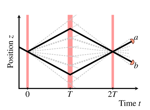
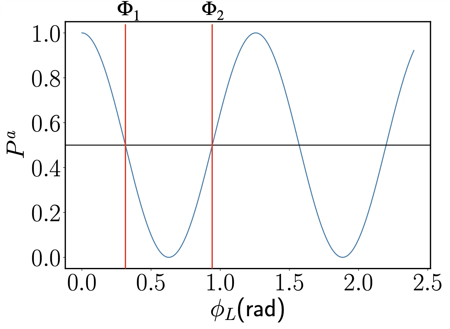
Figure 1: a) Multi-path nature of Bragg atom interferometer for a MZ interferometer, showing an $n$th-order Bragg beam splitter (BS) populating the main trajectories (solid black lines), open ports, and parasitic paths (dashed lines; the dominant ones for $n=5$ are thicker), all affecting the MZ signal recorded in ports a and b. Fig. adapted from Kirsten-Siemß et al. (2023). b) Extraction of the mid-fringes by solving $P_{a}(\Phi)=0.5$ where $P_{a}(\Phi)$ is the fitted two-mode estimator for the population in port a.

II Bragg Atom Interferometry

Bragg transitions are driven by elastic scattering from pulsed optical lattices. Two counter-propagating laser beams with wavevectors $\vec{k}=\vec{k}_{1}\simeq-\vec{k}_{2}$ form an optical lattice, $V(t,x)=\Omega(t)\cos^{2}{\{k[x-x_{\mathrm{L}}(t)]\}}$ Jackson (2009). Typically, the lasers are far detuned from any electronically excited states and couple the atom’s motional states with an effective two-photon Rabi frequency $\Omega(t)$ Müller et al. (2008). The lattice motion $x_{\mathrm{L}}(t)=\int^{t}_{0}\delta(\tau)/2k\;\mathrm{d}\tau+\phi_{L}(t)/k$ is a function of the laser frequency detuning $\delta(t)\equiv\omega_{1}(t)-\omega_{2}(t)$ and the relative laser phase $\phi_{L}(t)\equiv\phi_{1}(t)-\phi_{2}(t)$ Peik et al. (1997).

The pulsed Bragg lattice transfers multiple pairs of photon recoil $2n\hbar k$, where the integer $n$ is the Bragg order. When we expand the effective Hamiltonian in momentum eigenstates $\ket{2m\hbar k}$ for integer $m$ and move to a frame co-moving with the optical lattice, we obtain the following matrix elements Louie et al. (2023); Müller et al. (2008)

$$H_{m,l}/\hbar= [m^{2}\omega_{r}-\frac{m}{2}(4\omega_{r}\frac{p}{\hbar k}+\delta(t))]\delta_{m,l}$$

$$+\frac{\Omega(t)}{2}[e^{-\mathrm{i}\phi_{L}(t)}\delta_{m,l-2}+H.c.].$$ (1)

Here, $\omega_{r}\equiv\frac{\hbar k^{2}}{2M}$ is the recoil frequency of an atom with mass $M$. For a fixed even (odd) Bragg order $n$ we only consider matrix elements with even (odd) $m$. In addition, we account for a momentum offset $p$ between the lattice and the atoms, along with the resulting Doppler effects Szigeti et al. (2012). We assume that our initial atomic state has a Gaussian momentum distribution $\mathcal{N}(p,\sigma_{p})$, which, without loss of generality, is centered around $\ket{-n\hbar k}$ and has a width $\sigma_{p}$.

Both the intrinsic multipath nature of Bragg atom interferometry and the intrinsic momentum distribution of the incoming wave packet are accounted for by the Hamiltonian in Eq. (II). While it, in principle, describes the coupling of an infinite ladder of momentum states, it is sufficient to consider a finite truncated Hilbert space due to finite couplings strengths Müller et al. (2008); Siemß et al. (2020). Here, we include $n+1$ discrete momentum states ($\ket{-n\hbar k}$, $\ket{-(n-2)\hbar k}$, $\ket{-(n-4)\hbar k}$,…, $\ket{(n-2)\hbar k}$,$\ket{n\hbar k}$) in addition to three additional levels at each end ($\ket{-(n+6)\hbar k}$, $\ket{-(n+4)\hbar k}$, $\ket{-(n+2)\hbar k}$,$\ket{(n+2)\hbar k}$,…, $\ket{(n+6)\hbar k}$). Moreover, Eq. (II) reveals the control parameters to generate OCT pulses: The effective Rabi frequency, the relative laser phase, and the detuning: $\left(\Omega(t),\phi_{L}(t),\delta(t)\right)$.

In contrast to previous studies which were focused on improving the robustness of the interferometer against external noise sources Louie et al. (2023); Saywell et al. (2023); Li et al. (2024); Baker et al. (2025), we optimize these parameters to overcome the inherent multistate scattering of Bragg diffraction and express the gains in terms of the metrologically relevant diffraction phase.

III Pulse Optimization Method

Before evaluating the phase accuracy of the full OCT-enhanced Bragg interferometers, we optimize the individual beam-splitter and mirror operations making up the MZ in Fig. 1. Here, we investigate how well they mimic effective two-mode operations in the presence of a significant velocity dispersion of the atomic wave packet. In fact, we observed that the approach of optimizing beam splitters and mirrors independently before assembling the full atom interferometer yields overall better results than optimizing the entire system at once.

The OCT framework utilized in this study is Q-CTRL’s Boulder Opal package Ball et al. (2021). To quantify the improvements achieved by OCT optimization, we will compare it to pulses using optimized Gaussian temporal pulse shapes. While these pulses are more complex than traditional box pulses, it is well-established in Bragg interferometry that their smooth flanks reduce scattering losses Müller et al. (2008). As a baseline, we therefore run the optimizer with a fixed laser phase and detuning $\phi_{L}(t)=0=\delta(t)$, while we also set a Gaussian envelope for the effective Rabi frequency

$$\Omega(t)=\Omega_{0}e^{-t^{2}/2\tau^{2}}.$$ (2)

This configuration introduces two optimization parameters: the peak Rabi frequency $\Omega_{0}$ and the pulse width $\tau$. The duration of the Gaussian pulse will be truncated at $\pm 5\tau$.

In contrast, the optimization variables of the OCT pulses are $\Omega(t),\phi_{L}(t),\delta(t)$. We chose a total duration of $300\mu s$. To limit the maximum rate of change per time increment $\Delta t=1\mu s$, in which the individual parameters will be updated, we additionally impose cut-off frequencies of $95$ kHz and $80$ kHz for beam splitters and mirrors, respectively. This is done through a convolution of the optimization variables with a sinc kernel, $K(t)=\sin(\omega_{c}t)/\pi t$, defined by a cut-off frequency $\omega_{c}$. The sinc kernel in the frequency domain is constant in the range $[-\omega_{c},\omega_{c}]$ and zero elsewhere. This ensures that the optimized parameters remain within experimental constraints.

Ideally, the unitary time evolution operator for a two-mode beam splitter $\hat{U}_{\text{BS}}$ transfers the incoming state into an equal superposition, $\hat{U}_{\text{BS}}\ket{\mp n\hbar k}=\frac{1}{\sqrt{2}}\left(\ket{\mp n\hbar k}-\mathrm{i}\ket{\pm n\hbar k}\right)$. An ideal mirror reflects the momentum of the state, $\hat{U}_{\text{M}}\ket{\mp n\hbar k}=\ket{\pm n\hbar k}$. We will measure the performance of a given pulse by its distance to the target unitary $\hat{U}_{T}$, also referred to as fidelity,

$$\mathcal{F}\left(\hat{U}_{T}\right)=\frac{1}{N}\sum_{i=1}^{N}\frac{\|\mathrm{Tr}\left(\hat{U}_{T}^{\dagger}\hat{U}^{(i)}\right)\|}{\|\mathrm{Tr}\left(\hat{U}_{T}^{\dagger}\hat{U}_{T}\right)\|}.$$ (3)

The cost function for the optimization is then the corresponding infidelity

$$\text{cost}\left(\hat{U}_{T}\right)=\frac{1}{N}\sum_{i=1}^{N}1-\frac{1}{2}\|\mathrm{Tr}\left(\hat{U}_{T}^{\dagger}\hat{U}^{(i)}\right)\|.$$ (4)

In this equation, $\hat{U}_{T}$ are the respective target unitary operations, i.e., $\hat{U}_{\text{BS}}$ and $\hat{U}_{\text{M}}$. Robust control with respect to the finite momentum distribution of the incoming wave packet $\mathcal{N}(p,\sigma_{p})$ is achieved as we average the cost for a batch of unitaries $\hat{U}^{(i)}$, which are characterized by their momentum offset $p_{i}$ with $i=1,\dots,N$ in Eq. (II). For the results of the optimizations presented here, we consider wave packets with three different momentum widths $\sigma_{p}\in\{0.01,0.1,0.3\}\hbar k$, and sample them using batch sizes of $N=300$. To compare the performance of different OCT pulses we increase the number of samples to $N=4000$. Finally, in Sec. V, in order to reach resolutions of the interferometer fringe of up to a $\mu$rad, we require on the order of $10^{7}$ samples for the Gaussian momentum distribution.

Note, that we reduced the computational complexity of the optimization and evaluation of Eq. (4) by first projecting into the relevant two-mode subspace defined by the main momentum states $\ket{\mp n\hbar k}$ Saywell et al. (2023). Moreover, we recall that in certain interferometer geometries like the MZ in Fig. 1, the mirror pulse can serve a dual purpose by also deflecting incoming parasitic paths populated by the initial beam splitter Pfeiffer et al. (2025); Kirsten-Siemß et al. (2023). As we will see, this is particularly important when using Gaussian pulse shapes, as the beam splitters exhibit non-negligible populations in parasitic paths. Consequently, we include the proper weights for deflecting the first-order parasitic paths in the cost function in the case of the Gaussian mirror pulses.

IV Fidelity Analysis

IV.1 Single Pulse

First, we evaluate the residual coupling to parasitic momentum states of both Gaussian pulses with optimized parameters and OCT pulses. For all of the following results, we consider Bragg operations of orders $n=3$ and $n=5$. Furthermore, third-order Bragg pulses couple to only a single pair of intermediate states compared to fifth-order pulses, suggesting a potential trade-off between Bragg order and parasitic effects.

We start by discussing the population transfer of an incoming wave packet with momentum width $\sigma_{p}=0.1\hbar k$, interacting with a Bragg beam splitter of order five as depicted in Fig. 2. The plot shows the population distribution of the wave packet after the interaction with the beam splitter for both the Gaussian pulse parameters (top) and OCT pulses (bottom). As can be seen in Fig. 2(top) the population in the momentum state $\ket{-3\hbar k}$, which corresponds to one of the first parasitic paths, corresponds to about $10\%$ of the total population. This example illustrates clearly the challenge for traditional pulse shapes in maintaining high diffraction efficiencies while facing considerable velocity dispersion and scattering losses. It also demonstrates that even for a considerably narrow wave packet featuring $\sigma_{p}=0.1\hbar k$, the emerging parasitic populations are relevant. As mentioned in the previous section, we have modified the cost function in Eq. (4) for the Gaussian mirror pulses as detailed in App. B.

In contrast, the OCT population transfer for an incoming wave packet with momentum width $\sigma_{p}=0.1\hbar k$, interacting with a Bragg beam splitter of order five, shown in Fig. 2 (bottom), shows an almost perfect beam splitter with smooth Gaussian distributions of the populations in $\ket{\pm 5\hbar k}$ after the interaction. The corresponding pulse parameters for this OCT beam splitter are shown in Fig. 2. In App. A we also show and discuss other combinations of $\sigma_{p}$ and OCT/Gaussian optimizations, as well as Bragg orders $n=3$ and $n=5$, which illustrate that OCT may well suppress parasitic populations up to momentum widths of $\sigma_{p}=0.3\hbar k$.

With this comparison, we see a significantly better suppression of parasitic paths using the OCT pulses compared to the Gaussian pulses even at the level of the beam splitter, which will have a positive effect on the diffraction phase. Nevertheless, it is important to highlight that for $\sigma_{p}=0.3\hbar k$, the parasitic ports of the OCT pulse do not disappear completely (see App. A), and therefore colder clouds will have an advantage in terms of diffraction phase, as we will discuss in Sec. V.

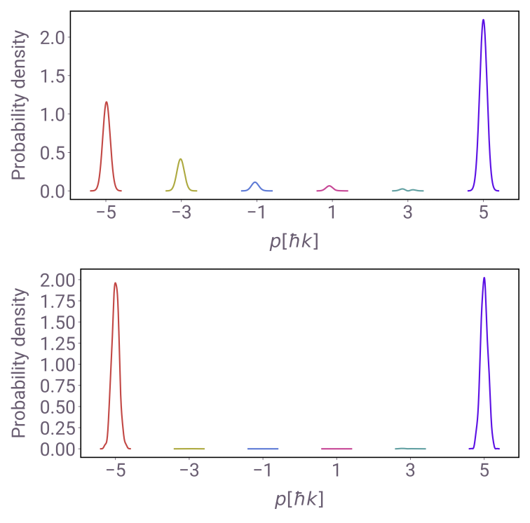
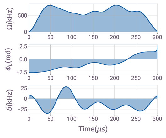
Figure 2: Study of an optimized beam splitter for the case of an initial state with momentum distribution of $\sigma_{p}=0.1\hbar k$ and Bragg order $n=5$. a) Top: Populations after the interaction with an optimal Gaussian pulse with a peak Rabi frequency of $\Omega_{0}=34\omega_{r}$ and a pulse width of $\tau=0.145\omega_{r}^{-1}$, where we have the relative populations in $\ket{5\hbar k}$ and $\ket{-5\hbar k}$ of $0.5458$ and $0.2848$, respectively. Bottom: Populations after the interaction with an optimal OCT pulse where we have the relative populations in $\ket{5\hbar k}$ and $\ket{-5\hbar k}$ of $0.4997$ and $0.4980$, respectively b) OCT pulse parameters where a cutoff frequency of $95$ kHz has been used for the optimization.

IV.2 Full Atom Interferometer

The previous discussion of a single beam splitter has shown that OCT pulses can reach considerably higher fidelities for single operations, especially for atomic clouds with significant velocity dispersion (cf. Saywell et al. (2023); Louie et al. (2023)). However, our focus is on suppressing the influence of parasitic paths on the signal of full interferometers. We recall that in these cases, later operations in the interferometer can be used to deflect parasitic paths Pfeiffer et al. (2025); Kirsten-Siemß et al. (2023). Hence, we compute the fidelity of multiple consecutive operations, $\mathcal{F}\left(\hat{U}_{T}\right)$ (3), composing the MZ interferometer as shown in Fig. 1. Here, $\hat{U}_{T}$ will correspond to the ideal beam splitter $\hat{U}_{BS}$, the ideal mirror $\hat{U}_{M}$, the ideal composite unitary after the mirror $\hat{U}_{M}\hat{U}_{BS}$ or the complete MZ unitary $\hat{U}_{BS}\hat{U}_{M}\hat{U}_{BS}$. Note that when calculating the fidelity for the composite unitary after the mirror and the complete MZ unitary, one must consider that momentum labels are not unique anymore, as multiple paths of the interferometer can have the same momentum. Therefore, one must account for this when defining these unitaries (See for example the supplement of Kirsten-Siemß et al. (2023)).

Table 1 shows the fidelity of each step in the MZ interferometer. For the case of a small momentum distribution, $\sigma_{p}=0.01\hbar k$, the fidelity of the Gaussian pulses and the OCT pulses are comparable for both Bragg orders, even though the OCT pulses still perform better. Towards larger momentum widths, OCT starts to show a significant improvement compared to the Gaussian pulses, both for the individual operations and for the combined full interferometer ideal unitary. The most notable difference is observed for a Bragg order of $n=5$ and a momentum width of $\sigma_{p}=0.1\hbar k$ where we have $\mathcal{F}=\{0.48,0.99\}$ for Gaussian and OCT-pulses, respectively. For the specific case of the mirror pulses, we can see that Gaussian pulses are capable of maintaining a high fidelity for $\sigma_{p}=0.1\hbar k$, but it drops considerably for $\sigma_{p}=0.3\hbar k$. Nevertheless, even for $\sigma_{p}=0.1\hbar k$ the full sequence is heavily affected by the performance of the beam splitter.

These results show how OCT pulses outperform Gaussian pulses if we want the interferometer to be as close as possible to a two-mode interferometer, i.e., achieving better suppression of parasitic paths and less sensitivity to velocity dispersion. Furthermore, we also observe that cooler clouds exhibit considerably better performance. To clarify what that means in terms of accuracy, we will now compute the diffraction phase of these interferometers.

		$n=3$		$n=5$
	$\sigma_{p}\;[\hbar k]$	Gaussian	OCT	Gaussian	OCT
	$0.01$	[head to column names]Newtabledata3U.csv	[head to column names]Newtabledata3U.csv	[head to column names]Newtabledata5U.csv	[head to column names]Newtabledata5U.csv
$\hat{U}_{\mathrm{BS}}$	$0.1$	[head to column names]Newtabledata3U.csv	[head to column names]Newtabledata3U.csv	[head to column names]Newtabledata5U.csv	[head to column names]Newtabledata5U.csv
	$0.3$	[head to column names]Newtabledata3U.csv	[head to column names]Newtabledata3U.csv	[head to column names]Newtabledata5U.csv	[head to column names]Newtabledata5U.csv
	$0.01$	[head to column names]Newtabledata3U.csv	[head to column names]Newtabledata3U.csv	[head to column names]Newtabledata5U.csv	[head to column names]Newtabledata5U.csv
$\hat{U}_{\mathrm{M}}$	$0.1$	[head to column names]Newtabledata3U.csv	[head to column names]Newtabledata3U.csv	[head to column names]Newtabledata5U.csv	[head to column names]Newtabledata5U.csv
	$0.3$	[head to column names]Newtabledata3U.csv	[head to column names]Newtabledata3U.csv	[head to column names]Newtabledata5U.csv	[head to column names]Newtabledata5U.csv
	$0.01$	[head to column names]Newtabledata3U.csv	[head to column names]Newtabledata3U.csv	[head to column names]Newtabledata5U.csv	[head to column names]Newtabledata5U.csv
$\hat{U}_{\mathrm{M}}\hat{U}_{\mathrm{BS}}$	$0.1$	[head to column names]Newtabledata3U.csv	[head to column names]Newtabledata3U.csv	[head to column names]Newtabledata5U.csv	[head to column names]Newtabledata5U.csv
	$0.3$	[head to column names]Newtabledata3U.csv	[head to column names]Newtabledata3U.csv	[head to column names]Newtabledata5U.csv	[head to column names]Newtabledata5U.csv
	$0.01$	[head to column names]Newtabledata3U.csv	[head to column names]Newtabledata3U.csv	[head to column names]Newtabledata5U.csv	[head to column names]Newtabledata5U.csv
$\hat{U}_{\mathrm{BS}}\hat{U}_{\mathrm{M}}\hat{U}_{\mathrm{BS}}$	$0.1$	[head to column names]Newtabledata3U.csv	[head to column names]Newtabledata3U.csv	[head to column names]Newtabledata5U.csv	[head to column names]Newtabledata5U.csv
	$0.3$	[head to column names]Newtabledata3U.csv	[head to column names]Newtabledata3U.csv	[head to column names]Newtabledata5U.csv	[head to column names]Newtabledata5U.csv

Table 1: Fidelity, as defined by Eq. (3), of a beam splitter, a mirror, their combination, or the full interferometer for optimal control pulses and optimized Gaussian pulses for Bragg orders $n=3$ and $n=5$ and an initial state with a momentum Gaussian distribution of width $\sigma_{p}$ centered around $\ket{-3\hbar k}$ and $\ket{-5\hbar k}$ respectively.

V Phase accuracy

The goal of this section is to assess the performance of the OCT pulses in terms of the phase accuracy of the MZ interferometer. We quantify it by computing the residual phase shift caused by the spurious couplings to unwanted momentum states, i.e., the Bragg diffraction phase Kirsten-Siemß et al. (2023); Parker et al. (2016); Béguin et al. (2022); Geiger et al. (2020); Plotkin-Swing et al. (2018); Estey et al. (2015); Büchner et al. (2003). In the absence of other phase contributions, we compute the diffraction phase, denoted as $\delta\Phi\equiv\Phi^{\text{measured}}-\Phi_{\mathrm{L}}$, by subtracting the control phase shift $\Phi_{\mathrm{L}}$, e.g., imprinted via the laser phase of the final pulse of the MZ, from the phase extracted from the interferometer signal $\Phi^{\text{measured}}$.

Atom interferometers encode the relative phase between the arms of the interferometer $\Phi$ in the populations of their output ports. The interferometer signal is typically defined as the relative atom numbers measured in the two main ports, e.g., $N_{a}$ and $N_{b}$ in Fig. 1,

$$P_{a}(\Phi)=\frac{N_{a}(\Phi)}{N_{a}(\Phi)+N_{b}(\Phi)}.$$ (5)

To extract the phase from population measurements, one must define an estimator that describes the functional relationship between these two quantities. In the case of ideal two-mode beam splitters and mirrors, this signal is a perfect cosine, $P_{a}(\Phi)\propto\cos{(\Phi)}$. This motivates the widespread use of the two-mode estimator

$$P_{a}(\Phi)=\frac{1}{2}\left(B+C\cos(n\Phi+A)\right),$$ (6)

where $P_{b}(\Phi)$ simply includes an offset of $\pi$ in the phase. The fit parameters in this formula are a shift in the phase $A$, an offset in the mean amplitude of the signal $B$ and its amplitude $C$. Varying the laser phase shift $\Phi_{\mathrm{L}}$ produces an oscillating signal as depicted in Fig. 1, to which the model in Eq. (6) is fit, calibrating the parameters $A,B$ and $C$. Finally, the estimated phase is a function of the measured populations and can be obtained by inverting the calibrated signal model $\Phi^{\text{measured}}={P^{-1}}_{a}(P^{\text{measured}}_{a})$. Yet, the scattering to spurious states gives rise to a more complex signal in Bragg atom interferometers than the one in Eq. (6)  Altin et al. (2013). Applying a more complex estimator model, which accounts for all possible Fourier components in the interferometer signal, would be challenging to implement in an experiment. This is due to the large number of parameters involved and the difficulty of detecting a very small number of atoms per port. Implementing the model in Kirsten-Siemß et al. (2023), which accounts for a few Fourier components, would assume a mirror interaction transparent for the main parasitic paths. Instead of these approaches, we proceed to quantify the residual errors in terms of $\delta\Phi$ when using the OCT pulses found in the previous section.

We simulate the signal fringes for the MZ interferometer for Bragg orders $n=3,5$ by scanning 50 discrete values for the laser phase $\phi_{\mathrm{L}}\in[0,2.4]$ rad via the second beam splitter in Fig. 1. For each $\phi_{\mathrm{L}}$, we then average over $N=24\cdot 10^{6}$ samples picked from the momentum distribution of the incoming wave packet. This is necessary to ensure sub-mrad phase resolution of the interferometer fringes. After calibrating $P_{a}(\Phi)$ in Eq. (6) based on this data, we proceed to evaluate $\delta\Phi$ at the center of the fringe as sketched in Fig. 1, where the signal is maximally sensitive to changes in the phase. We determine the two first mid-fringe positions $\Phi_{\mathrm{L},1}$ and $\Phi_{\mathrm{L},2}$ with $P_{a}(\Phi_{\mathrm{L},i})=0.5$ as highlighted in the figure. Computing $\Phi^{\text{measured}}$ with the same resolution of the wave packet’s momentum distribution as before then gives the diffraction phase $\delta\Phi_{i}=\Phi^{\text{measured}}_{i}-\Phi_{\mathrm{L},i}$ at these points, this is what we will call measurement in Fig. 3 and Fig. 4. The necessity to average over $N=24\cdot 10^{6}$ samples in order to properly describe the incoming momentum wavepacket brings some light on why optimizing individual operations worked better than trying to optimize the full atom interferometer.

To determine the phase accuracy of the OCT-enhanced Bragg interferometer, we determine the residual oscillation in the diffraction phase upon varying the time between the pulses, denoted as $T$ in Fig. 1. This $T$-dependence of the interferometer signal due to the emergence of parasitic interferometers introduces potentially challenging systematic errors due to aliasing effects Parker et al. (2016); Kirsten-Siemß et al. (2023). For the Bragg orders under consideration, the interference between the main parasitic paths and the main paths of the interferometers are described by oscillating terms due to the different accumulated phase with frequencies $8\omega_{r}(n+1)$ and $8\omega_{r}(n-1)$ Altin et al. (2013); Kirsten-Siemß et al. (2023)

$$\delta\Phi= \xi_{0}+\xi_{1}\cos{((n-1)8\omega_{r}T+\nu_{1})}$$

$$+\,\xi_{2}\cos{((n+1)8\omega_{r}T+\nu_{2})}.$$ (7)

Here, $\xi_{i}$ and $\nu_{i}$ are free fit parameters. We compute $\delta\Phi$ at the two mid-fringe positions for 24 values of $T\in[10,10.016]\;\mathrm{ms}$ to resolve one full oscillation period determined by $(n\pm 1)8\omega_{r}$, and consider the specific case of ⁸⁷Rb as an example.

Fig. 3 shows the diffraction phase $\delta\Phi$ for Bragg order $n=3$, when scanning $T$ in the MZ interferometer. The top row displays the results for momentum widths $\sigma_{p}\in\{0.01,0.1,0.3\}\hbar k$ for $\Phi_{\mathrm{L},1}$, while the bottom row is obtained with $\Phi_{\mathrm{L},2}$. Scanning $T$, we observe residual oscillations in $\delta\Phi$. These oscillations are strongly suppressed by the use of OCT pulses, showing a peak-to-peak diffraction phase value for $\sigma_{p}=0.01\hbar k$ of a few $\mu$rad for the first fringe and below $\mu$rad for the second fringe. For $\sigma_{p}=0.1\hbar k$, we have a peak-to-peak diffraction phase below $m$rad. The perfect fit of Eq. (V) confirms that the diffraction phase oscillations originate from the residual couplings. For the case of $\sigma_{p}=0.3\hbar k$, we maintain a peak-to-peak diffraction phase of a few $m$rad, showing good performance even for relatively wide momentum distributions of the wavepacket. Nevertheless, for this case and $\Phi_{\mathrm{L},2}$, we have an almost $100$ mrad offset, which probably comes from a residual deformation of the fringe not captured by the signal model in Eq. (6), which makes the fit of Eq. (V) good but not perfect. In the caption, we can also see the ratio of the population in the output ports with respect to the population of the incoming wave packet, which is normalized to $1$, defined as $P_{\text{out}}=N_{a}+N_{b}$, which corresponds to the fraction of atoms that contribute to the interferometric signal.

Fig. 4 is identical to Fig. 3 but for $n=5$. Overall, we see the same behavior, with peak-to-peak values of a few $\mu$rad, below mrad, and a few mrad, respectively, for $\sigma_{p}=[0.01,0.1,0.3]\hbar k$. For $\sigma_{p}=0.01\hbar k$, we can compare with the results shown in Ref. Kirsten-Siemß et al. (2023) for Gaussian pulses utilizing the so-called magic mirror. We obtain a better diffraction phase by a factor of around 8 and 100, respectively, for $\phi_{L,2}$ and $\phi_{L,1}$, with the advantage that we used a simpler estimator to fit the interferometer signal. For $\sigma_{p}=0.3\hbar k$, the fit is closer to all the simulated experiments (empty dots) compared to the case of Bragg diffraction $n=3$, but we still have an offset of about $52$ mrad.

We showed that OCT pulses allow for $\mu$rad level of phase control if the sample does not feature velocity dispersions with $\sigma_{p}\leq 0.1\hbar k$. This can set the requirements on the control of the velocity dispersion to ensure $\mu$rad-level phase control. This is true not only for the peak-to-peak oscillations but also for the absolute shift. For $\sigma_{p}=0.3\hbar k$, OCT pulses still suppress peak-to-peak oscillations to a few mrad, achieving good contrast, stability, and ratio of atoms that contribute to the interferometer signal. However, the fringe is still somewhat deformed compared to the two-mode model, leading to the different offsets, especially for $\Phi_{\mathrm{L},2}$. The fact that the error of the fit to a two-level system is on the order of $\approx 10^{-7}$, $10^{-5}$ and $10^{-4}$ respectively for $\sigma_{p}=[0.01,0.1,0.3]\hbar k$ indicates that the phase control afforded by the OCT pluses extends over the entire fringe.

$\sigma_{p}=0.01\hbar k$

$\sigma_{p}=0.1\hbar k$

$\sigma_{p}=0.3\hbar k$

$\Phi_{1}$

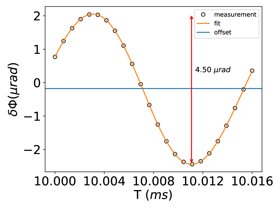
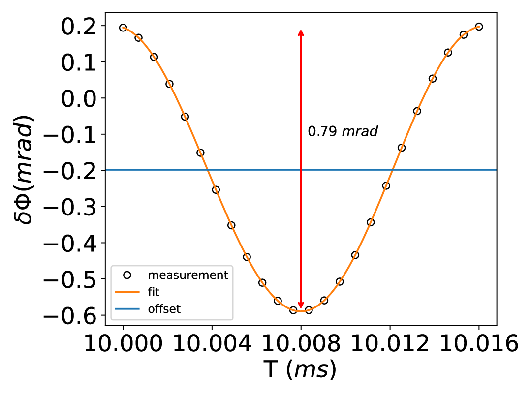
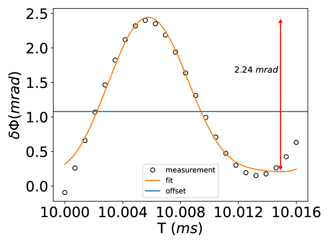
$\Phi_{2}$

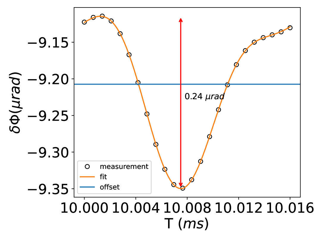
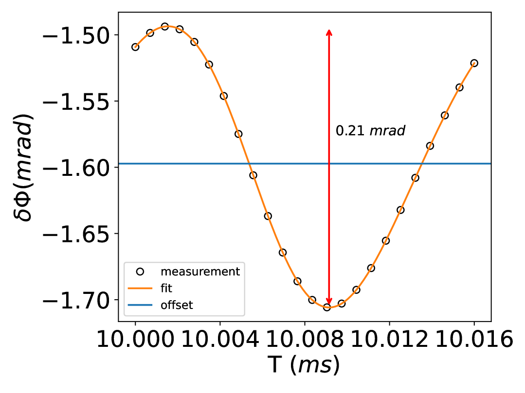
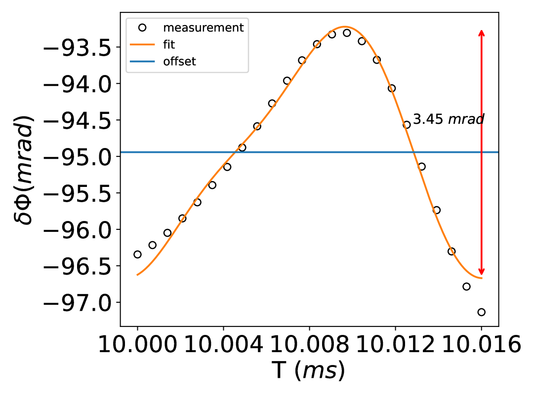
Figure 3: Diffraction phase for Bragg diffraction order $n=3$. The first and second rows represent the diffraction phase in the first and second mid-fringe, respectively. The columns from left to right represent the values of $\sigma_{p}=[0.01,0.1,0.3]\hbar k$. The blue line in each plot corresponds to a systematic phase shift, the empty circles are the simulated measurements, and the orange curve is the fit to Eq. (V). We see very small residual diffraction phase oscillations, demonstrating the performance of OCT pulses. For the cases of $\sigma_{p}=[0.01,0.1,0.3]\hbar k$, the populations and contrast $(P_{\text{out}},C)$ are $(0.99998,0.99997)$, $(0.99309,0.99567)$ and $(0.87722,0.70157)$, respectively.

$\sigma_{p}=0.01\hbar k$

$\sigma_{p}=0.1\hbar k$

$\sigma_{p}=0.3\hbar k$

$\Phi_{1}$

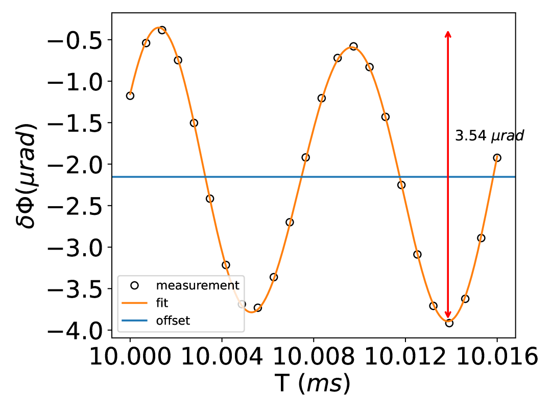
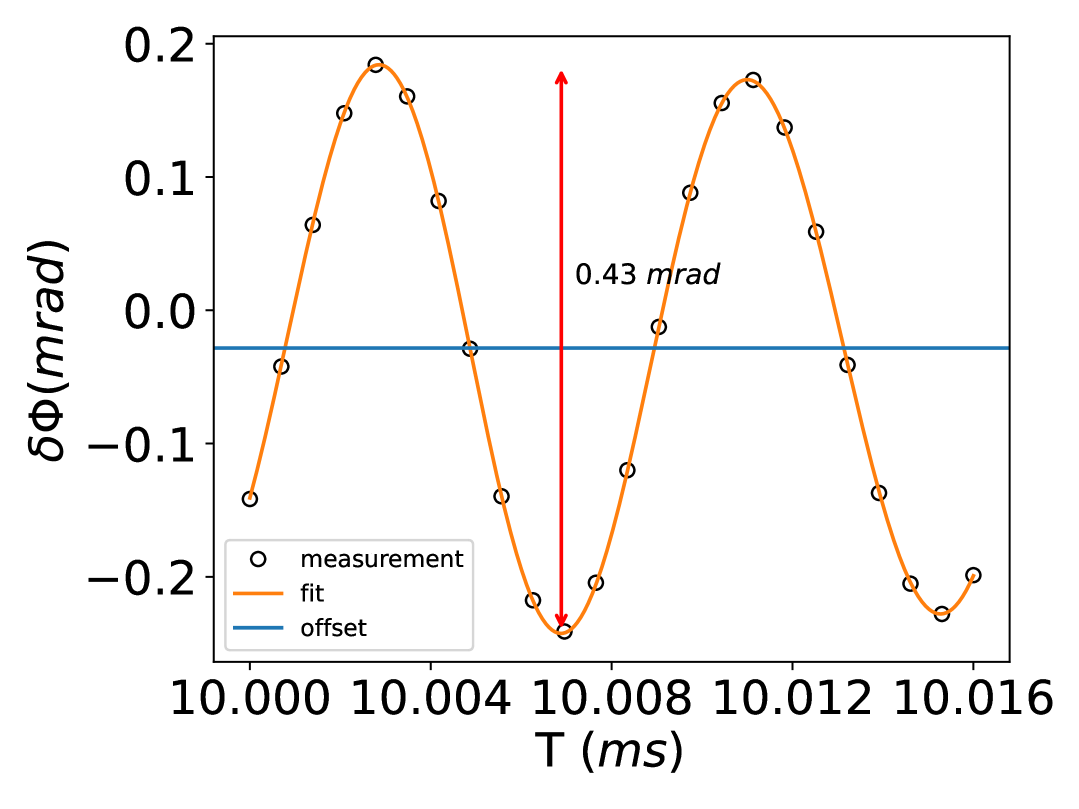
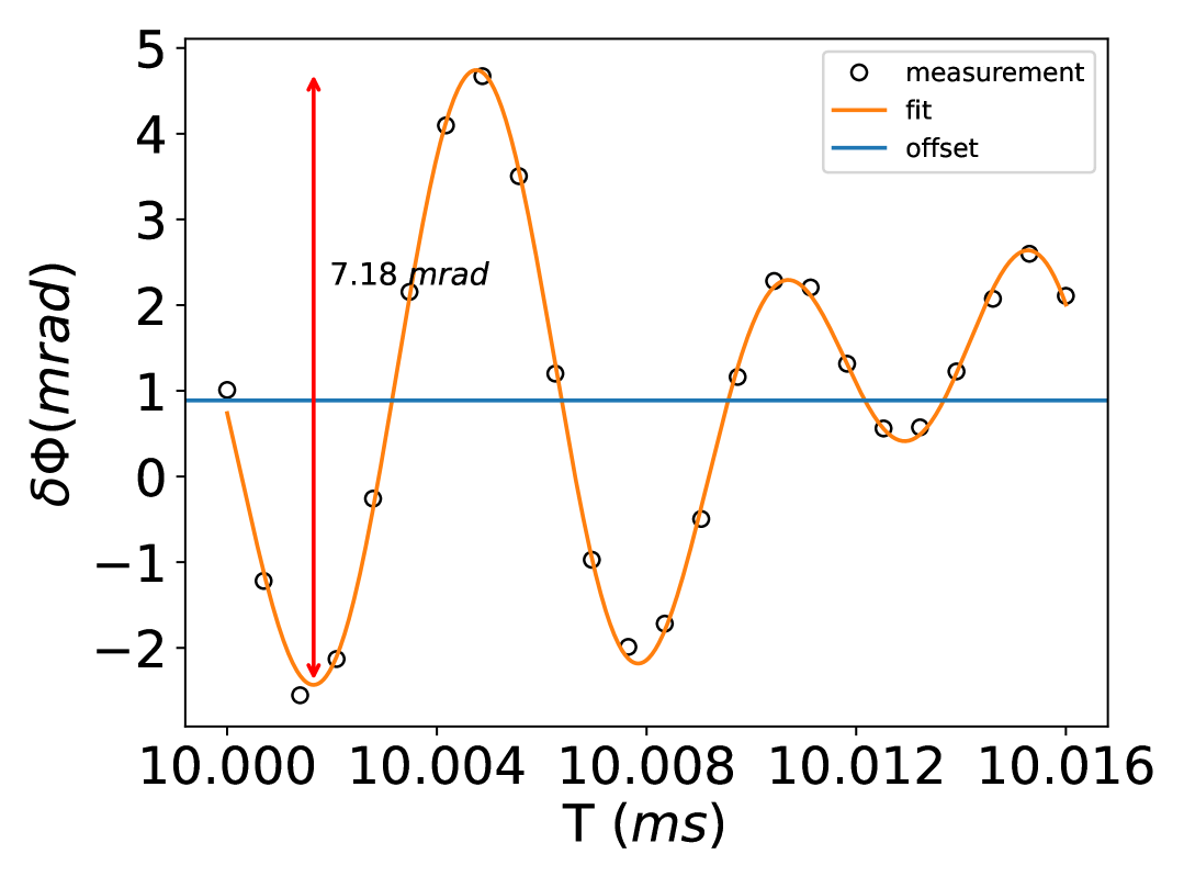
$\Phi_{2}$

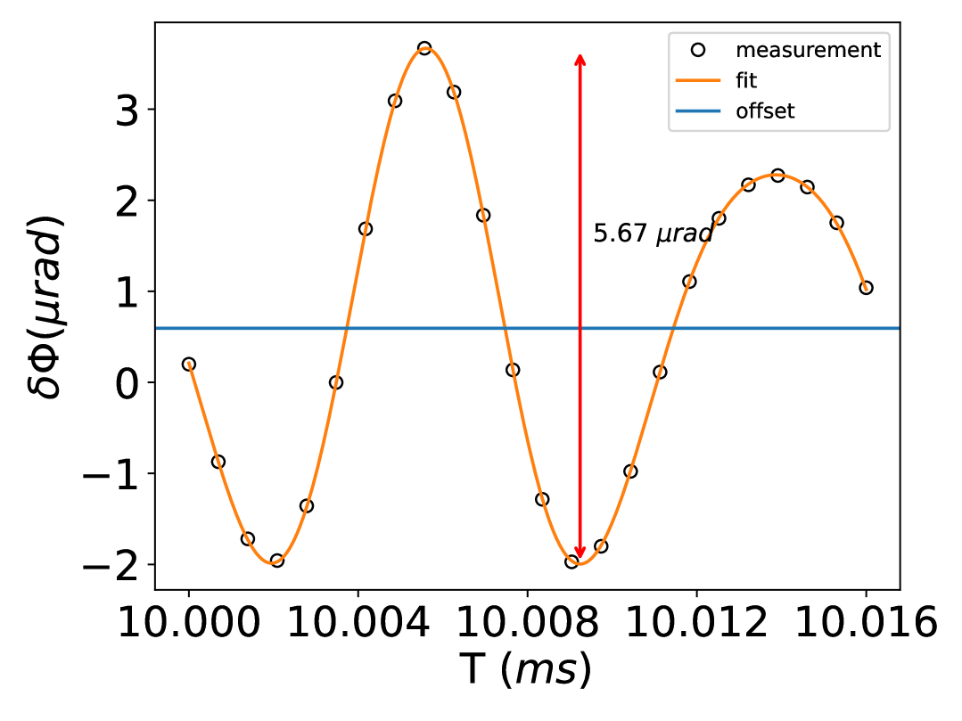
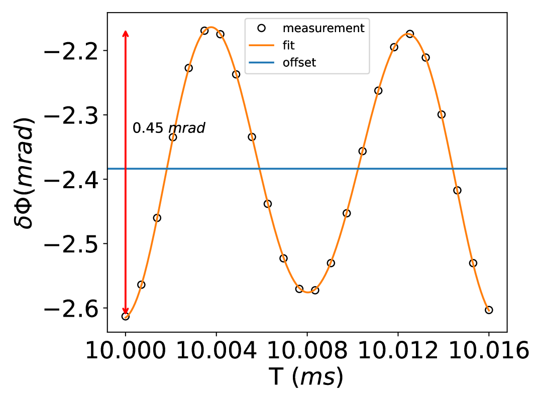
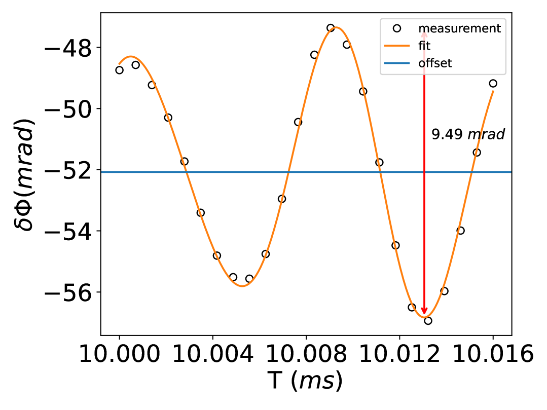
Figure 4: Diffraction phase for Bragg diffraction order $n=5$. The first and second rows represent the diffraction phase in the first and second mid-fringe, respectively. The columns from left to right represent the values of $\sigma_{p}=[0.01,0.1,0.3]\hbar k$. The blue line in each plot corresponds to the shift of the model, the empty circles are the measurements, and the orange curve is the fit to Eq. (V). We see very small residual diffraction phase oscillations, demonstrating the performance of OCT pulses. For the cases of $\sigma_{p}=[0.01,0.1,0.3]\hbar k$, the populations and contrast $(P_{\text{out}},C)$ are $(0.99994,0.99997)$, $(0.99157,0.98874)$ and $(0.78424,0.69266)$, respectively.

VI Conclusions

In this work, we demonstrated the metrological relevance of OCT-enhanced pulses by studying their use in the suppression of diffraction phases in high-order Bragg diffraction processes. So far, such pulses were promoted in the context of simply enhancing the contrast of atom interferometers. We showed the potential of ideally restoring a two-mode interferometry operation even for fundamentally multi-path, multi-port phenomena as the Bragg diffraction at high order. This brings this class of interferometers to the same level of their counterparts in the Raman regime, so far considered as more immune to transitions to unwanted states.

We have benchmarked the performance of 3rd- and 5th-order Bragg beam splitters and mirrors using OCT pulses against Gaussian pulses with optimized parameters. Here, we found that while the fidelity of Gaussian pulses suffers significantly due to both the coupling to unwanted states as well as a finite velocity width of the atomic ensemble, OCT pulses ensure good diffraction efficiencies.

We found that OCT pulses generally suppress diffraction phases below the $\mu$rad level for sufficiently cold clouds, achieving peak-to-peak values of a few $\mu$rad or below for $\sigma_{p}=0.01\hbar k$ and growing only to a few $m$rad if we account for temperatures up to $\sigma_{p}=0.3\hbar k$. Furthermore, this phase control extends over the entire fringe.

Our work contributes to the pursuit of atom interferometers with $\mu$rad precision, which is a requirement for applications such as gravitational wave detection Abdalla et al. (2025).

Appendix A Comparison of population transfer for different cases

In Sec. IV.1, we compared the population transfer of an incoming state with momentum width $\sigma_{p}=0.1\hbar k$ and Bragg order $n=5$ using an optimized Gaussian pulse and an OCT pulse. For completeness, we present in this appendix the population transfer for all pairs of $\sigma_{p}=[0.01,0.1,0.3]\hbar k$ and Bragg orders $n=[3,5]$ examined in this article, for both optimized Gaussian pulses and OCT pulses, and for both mirrors and beam splitters.

In Fig. 5( 7), we show the momentum distribution of an incoming state $\ket{-3\hbar k}$($\ket{-5\hbar k}$) after interacting with the laser generating a mirror. The first row corresponds to the optimized Gaussian pulse, and the second row correspond to the OCT pulse. Each column shows a different value of the momentum width distribution of the incoming state $\sigma_{p}$. We observe how the OCT pulses achieve a better population transfer: for $\sigma_{p}=0.01\hbar k$, the difference is small, but it exceeds $20\%$($25\%$) for $\sigma_{p}=0.3\hbar k$.

In Fig. 6( 8), we illustrate the momentum distribution of an incoming state $\ket{-3\hbar k}$($\ket{-5\hbar k}$) after interacting with the laser generating a beam splitter. The first row corresponds to the optimized Gaussian pulse, and the second row corresponds to the OCT pulse. Each column shows a different value of the momentum width distribution of the incoming state $\sigma_{p}$. We observe how the OCT pulses are closer to achieving an equally split population between the main ports. The momentum distribution for OCT pulses is a smooth Gaussian, in relation to p, for $\sigma_{p}=[0.01,0.1]\hbar k$, but deviates from that shape for $\sigma_{p}=0.3\hbar k$. Moreover, it presents a considerable amount of population in the parasitic ports. In the Gaussian case, for $\sigma_{p}=0.3\hbar k$ it is also noteworthy that the optimizer of the Gaussian pulse attempts to on average produce the behaviour of a beam splitter by creating a "bad" mirror, as can bee seen from the momentum selectivity of the pulse.

$\sigma_{p}=0.01\hbar k$

$\sigma_{p}=0.1\hbar k$

$\sigma_{p}=0.3\hbar k$

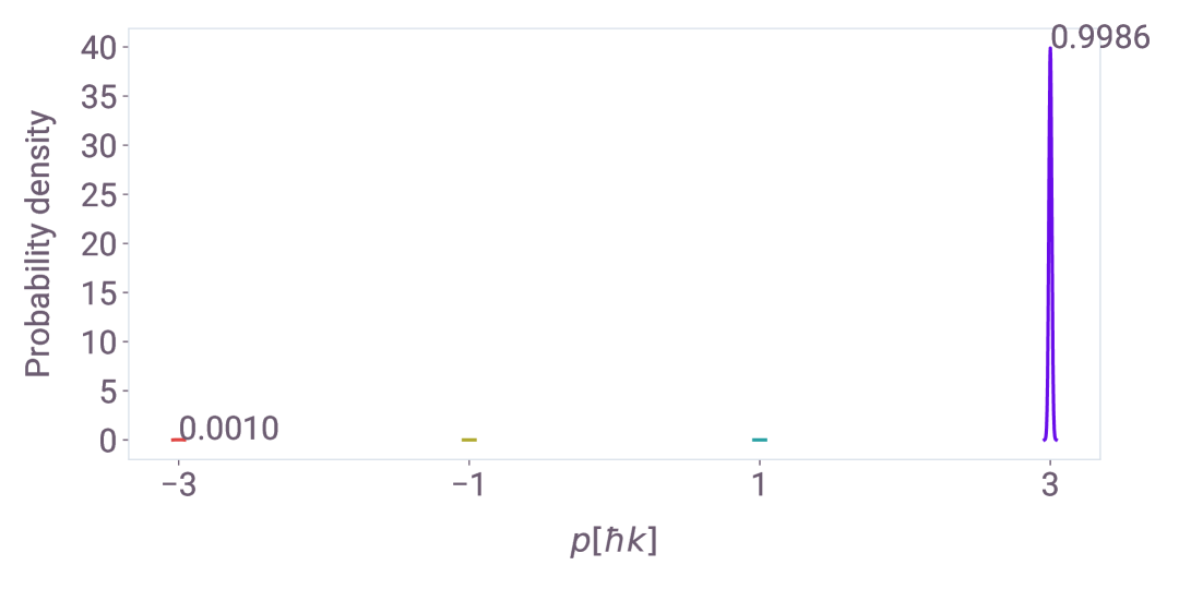
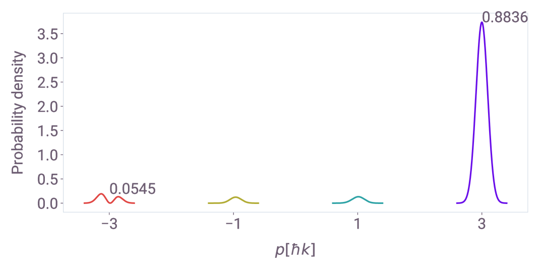
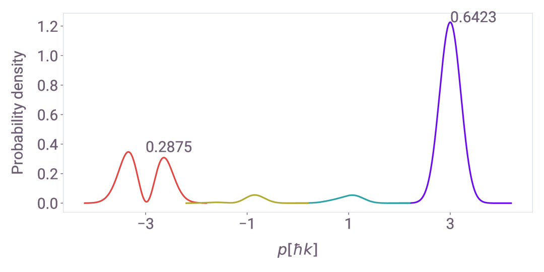
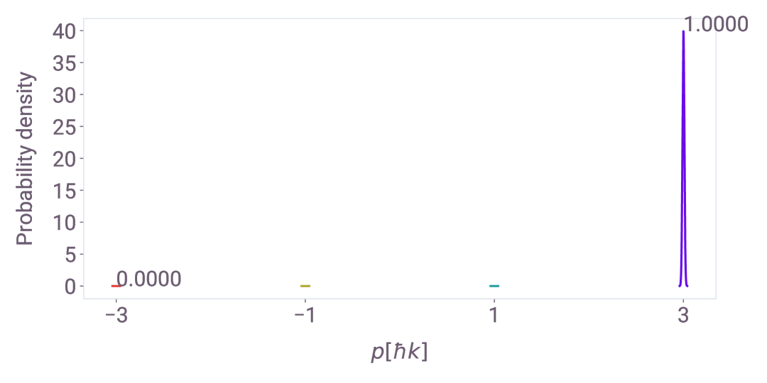
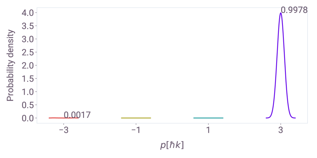
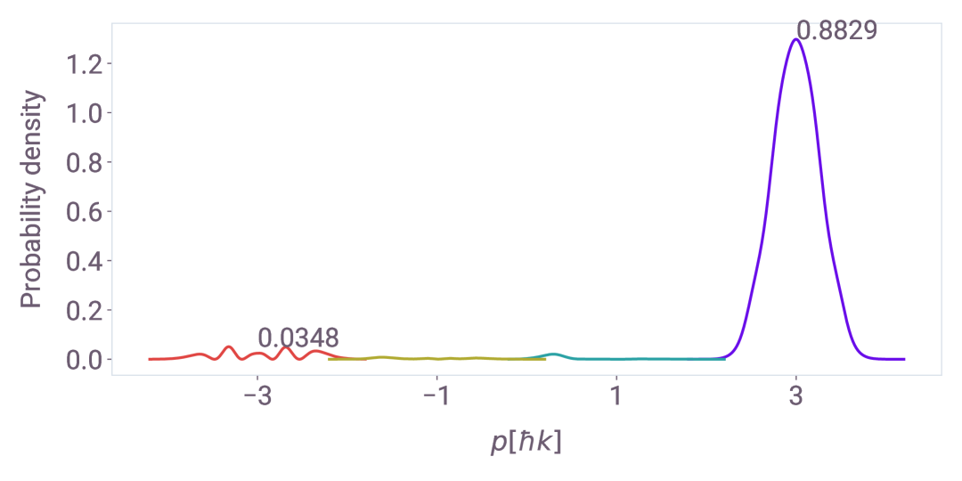
Figure 5: Momentum distribution of an incoming state $\ket{-3\hbar k}$ after interacting with the laser generating a mirror pulse. The first row is the result for a Gaussian-optimized pulse and the second row is for an OCT pulse. The columns correspond to $\sigma_{p}=[0.01,0.1,0.3]\hbar k$, respectively. The populations values of the main ports are shown in the figures. The Gaussian pulse parameters are, in order, for the first row $\left(\Omega,\tau\right)=\{\left(12.81,0.463\right),\left(14.52,0.349\right),\left(15.09,0.337\right)\}$, where $\Omega$ is in units of $\omega_{r}$ and $\tau$ is in units of $\omega_{r}^{-1}$.

$\sigma_{p}=0.01\hbar k$

$\sigma_{p}=0.1\hbar k$

$\sigma_{p}=0.3\hbar k$

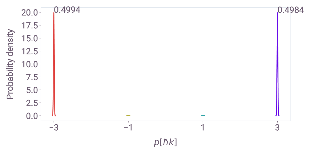
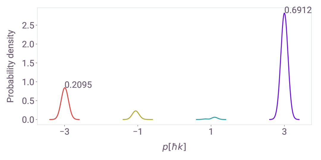
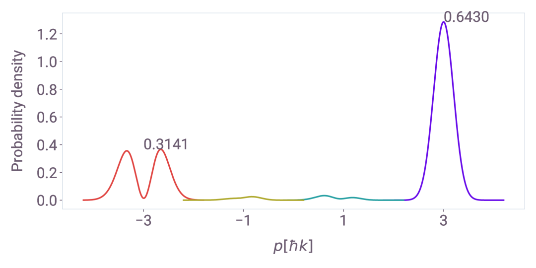
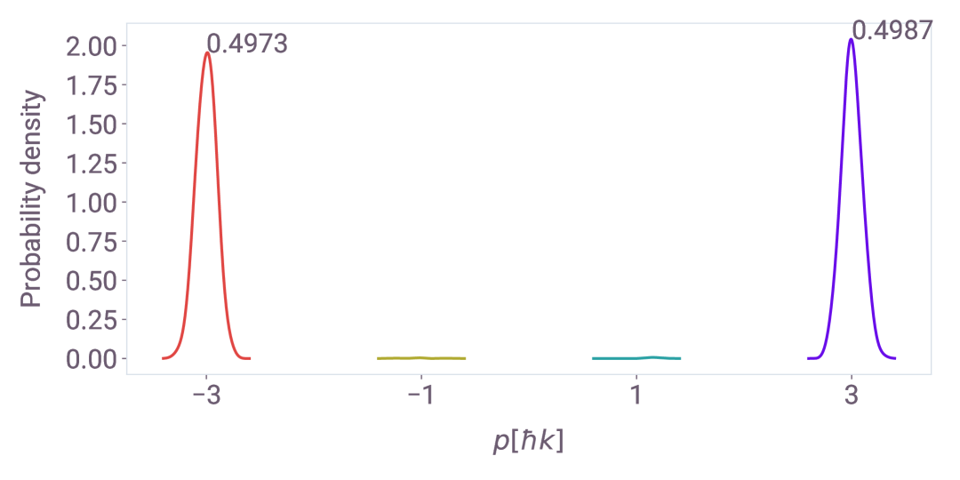
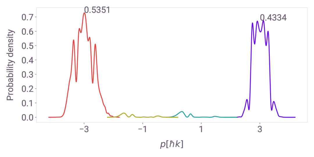
Figure 6: Momentum distribution of an incoming state $\ket{-3\hbar k}$ after interacting with the laser generating a beam splitter pulse. The first row is the result for a Gaussian-optimized pulse and the second row is for an OCT pulse. The columns correspond to $\sigma_{p}=[0.01,0.1,0.3]\hbar k$, respectively. The populations values of the main ports are shown in the figures. The Gaussian pulse parameters are, in order, for the first row $\left(\Omega,\tau\right)=\{\left(11.27,0.266\right),\left(15.59,0.178\right),\left(14.50,0.374\right)\}$, where $\Omega$ is in units of $\omega_{r}$, and $\tau$ is in units of $\omega_{r}^{-1}$.

$\sigma_{p}=0.01\hbar k$

$\sigma_{p}=0.1\hbar k$

$\sigma_{p}=0.3\hbar k$

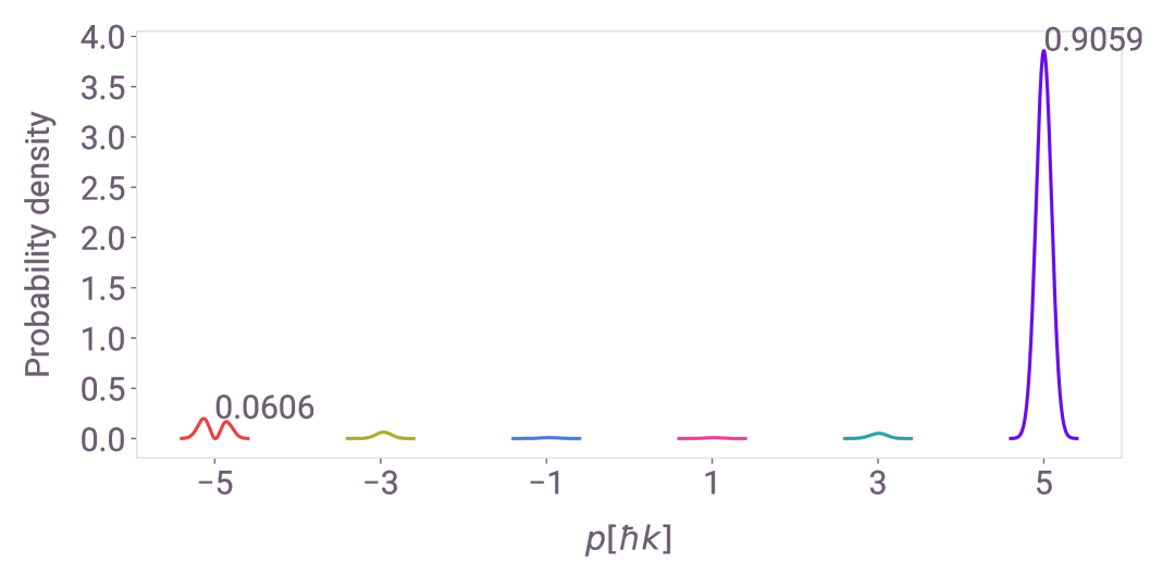
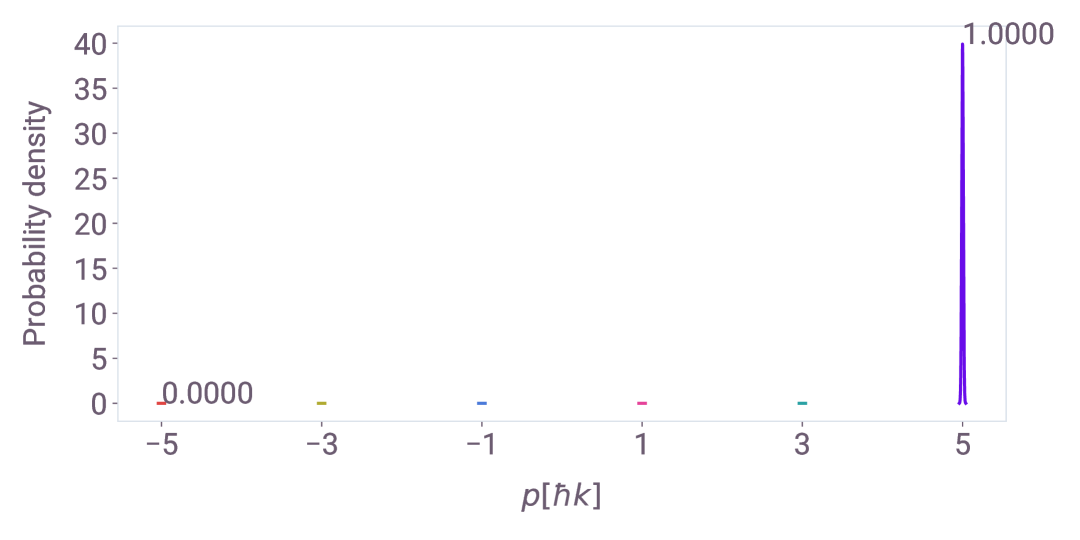
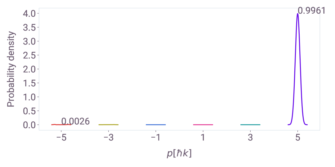
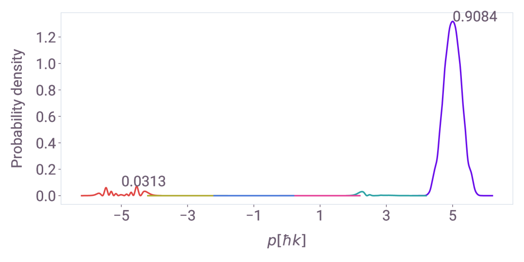
Figure 7: Momentum distribution of an incoming state $\ket{-5\hbar k}$ after interacting with the laser generating a mirror pulse. The first row is the result for a Gaussian-optimized pulse and the second row is for an OCT pulse. The columns correspond to $\sigma_{p}=[0.01,0.1,0.3]\hbar k$, respectively. The populations values of the main ports are shown in the figures. The Gaussian pulse parameters are, in order, for the first row $\left(\Omega,\tau\right)=\{\left(33.69,0.382\right),\left(35.86,0.308\right),\left(36.94,0.292\right)\}$, here $\Omega$ is in units of $\omega_{r}$ and $\tau$ is in units of $\omega_{r}^{-1}$.

$\sigma_{p}=0.01\hbar k$

$\sigma_{p}=0.1\hbar k$

$\sigma_{p}=0.3\hbar k$

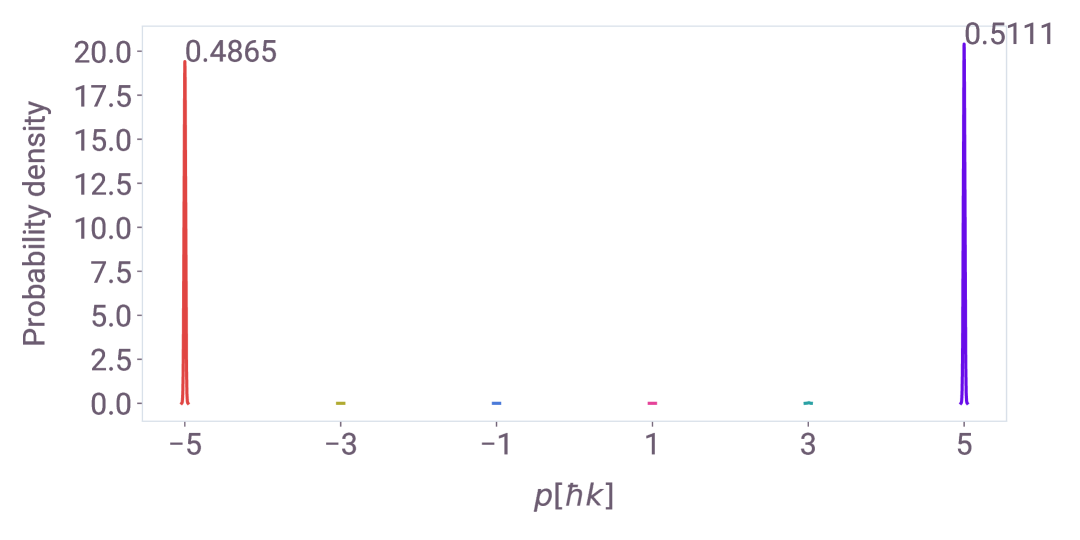
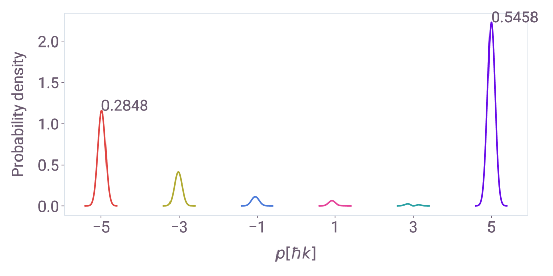
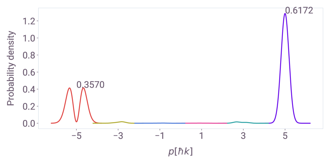
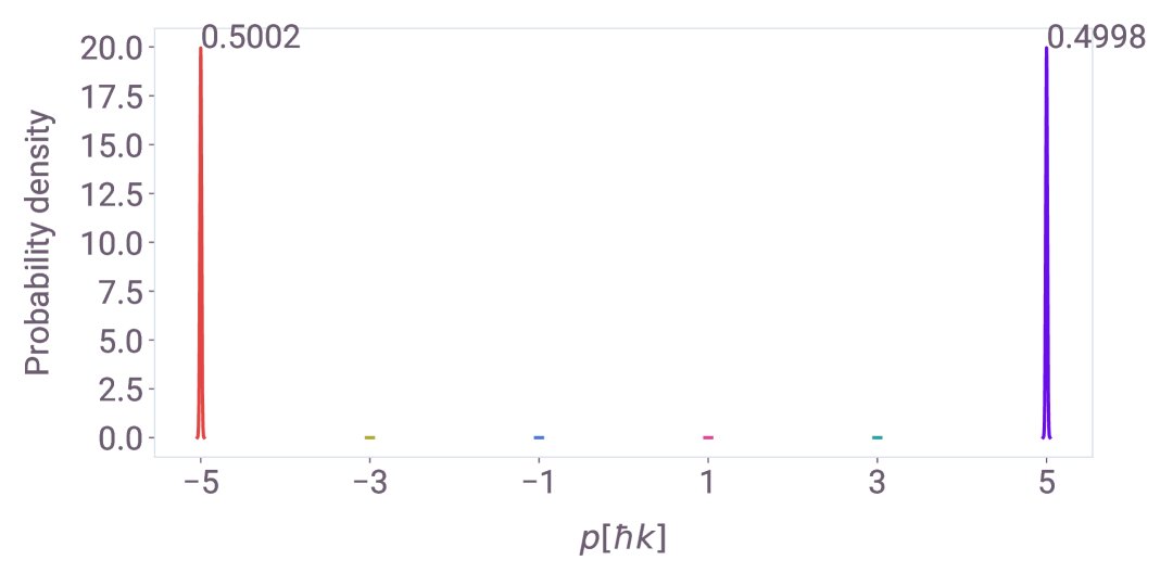
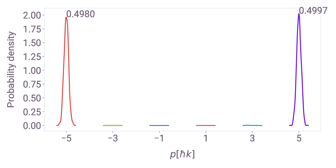
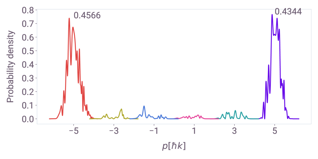
Figure 8: Momentum distribution of an incoming state $\ket{-5\hbar k}$ after interacting with the laser generating a beam splitter pulse. The first row is the result for a Gaussian-optimized pulse and the second row is for an OCT pulse. The columns correspond to $\sigma_{p}=[0.01,0.1,0.3]\hbar k$, respectively. The populations values of the main ports are shown in the figures. The Gaussian pulse parameters are, in order, for the first row $\left(\Omega,\tau\right)=\{\left(31.06,0.211\right),\left(34,0.145\right),\left(34,0.336\right)\}$, where $\Omega$ is in units of $\omega_{r}$ and $\tau$ is in units of $\omega_{r}^{-1}$.

Appendix B Cost function for Gaussian case Mirror

We have motivated in the main text, and further confirmed in the previous section, that the population in the parasitic ports after the first beam splitter is substantial for the optimized Gaussian pulses. Therefore, this had to be taken into account for the optimization of the mirror pulse. This was done by weighting the population of the parasitic ports for each optimization in the following way:

$$\text{cost}\left(\hat{U}_{T}\right)= \frac{1}{N}\sum_{i=1}^{N}1-\frac{1}{2}\|\mathrm{Tr}\left(\hat{U}_{T}^{\dagger}\hat{U}^{(i)}\right)\|$$

$$+W\frac{1}{2}\|\mathrm{Tr}\left(\hat{\mathcal{U}}_{T}^{\dagger}\hat{\mathcal{U}}^{(i)}\right)\|,$$ (8)

where $W$ corresponds to the cost associated to the optimization of the corresponding beam splitter for the same $\sigma_{p}$ and $\mathcal{U}$ corresponds to the ideal mirror interaction for the main parasitic ports.