BLUE: Bi-layer Heterogeneous Graph Fusion Network for Avian Influenza Forecasting

Abstract

Accurate forecasting of avian influenza outbreaks within wild bird populations requires models that account for complex, multi-scale transmission patterns driven by various factors. Spatio-temporal GNN-based models have recently gained traction for infection forecasting due to their ability to capture relations and flow between spatial regions, but most existing frameworks rely solely on spatial connections and their connections. This overlooks valuable genetic information at the case level, such as cases in one region being genetically descended from strains in another, which is essential for understanding how infectious diseases spread through epidemiological linkages beyond geography. We address this gap with BLUE, a Bi-Layer heterogeneous graph fUsion nEtwork designed to integrate genetic, spatial, and ecological data for accurate outbreak forecasting. The framework 1) builds heterogeneous graphs from multiple information sources and multiple layers, 2) smooths across relation types, 3) performs fusion while retaining structural patterns, and 4) predicts future outbreaks via an autoregressive graph sequence model that captures transmission dynamics over time. To facilitate further research, we introduce Avian-US dataset, the dataset for avian influenza outbreak forecasting in the United States, incorporating genetic, spatial, and ecological data across locations. BLUE achieves superior performance over existing baselines, highlighting the value of incorporating multi-layer information into infectious disease forecasting.

1 Introduction

Predicting the transmission of avian influenza remains a critical challenge in epidemiological research, due to the virus’s capacity for widespread dissemination among avian populations. Increasing cross-species transmission poses serious risks to public health infrastructure and global biosecurity. Accurately predicting where outbreaks may occur is vital for initiating early interventions that reduce infection risk and prevent spillover. To enable timely intervention and reduce the risk of zoonotic spillover, it is essential to identify high-risk regions prior to outbreak emergence (Caliendo et al., 2022; Prosser et al., 2024).

Earlier epidemiological models primarily adopt mechanistic strategies based on biological assumptions, often structured around fixed compartments such as SIR or SEIR (Geng et al., 2021; Della Marca et al., 2023). While effective in simplified scenarios, they lack network topology and interaction semantics (Hunter and Kelleher, 2022) as they both, in the deterministic form, work under low-dimensional Ordinary Differential Equation (ODE) systems that track infected counts in discrete disease states, thus falling short in representing the time-sequence reasoning and inter-location impact seen in real-world disease transmission.

To address the limitations of traditional epidemiological models, recent approaches have incorporated temporal architectures with Graph Neural Networks (GNNs) to capture spatio-temporal transmission dynamics from observational data (Liu et al., 2024). These models identify topological patterns both within and across time steps, enabling the learning of temporal correlations across spatially distributed locations in graph structures. This formulation offers a flexible and data-driven framework for supporting decision-making in disease surveillance and control, representing a significant advancement over classical forecasting methods (Brüel Gabrielsson, 2020; Liu et al., 2024). For example, Cola-GNN (Deng et al., 2020) captures the influence between the locations by combining the attention matrix with the geographical adjacency matrix. MSDNet (Tang et al., 2023) enhances regional epidemic predictions by integrating large-scale mobility data and fine-grained contact patterns through spatiotemporal graph learning.

Nevertheless, existing models follow a homogeneous setup, where nodes represent locations and are connected based on a static predefined adjacency matrix (Liu et al., 2023a; Yu et al., 2023; Lin et al., 2023) or a data-driven learnable correlations (Nguyen et al., 2023; Pu et al., 2024). These models overlook the role of individual infection cases and dynamics of transmission, reducing the complexity of avian influenza spread to spatial relationships between locations only. This simplification assumes that geographic or ecological proximity implies ongoing transmission risk, overlooking case-to-case interactions and temporal variability that often drive outbreak dynamics. Furthermore, it also treats all infected cases as equally infectious, ignoring subclade-specific transmission patterns and mutation-driven variation in virulence. As a result, current models struggle to capture detailed transmission patterns, particularly how individual cases interact both within and across geographic regions.

Although recent efforts bring in meteorological variables (Lim et al., 2021; Papagiannopoulou et al., 2024) or integrate GNNs with mechanistic components (Cao et al., 2022; Wang et al., 2022a; Sha et al., 2021), they still operate under a homogeneous graph structure based on spatial locations. This limits their ability to model fine-grained case-level interactions critical to understanding the spread of avian influenza. Differently, genetic correlations can offer an epidemiologically informative view by capturing infection-driven linkages that are invisible to spatial or ecological proximity alone. By modeling cases and locations as distinct node types and constructing edges based on both spatial and genetic relations, the problem transfers from standard homogeneous GNNs to heterogeneous GNNs (HGNNs) (Zhang et al., 2019). HGNNs support multiple node and edge types, and are better equipped to handle multi-relational, multi-typed graphs, making them highly suitable for epidemiological modeling. Although prior works considering combining multi-type information (Hemker et al., 2024; Kim et al., 2023; Yu et al., 2022; Guo et al., 2023), they typically perform as a static multi-modal disease diagnosis for cases, ignoring the temporal patterns. These methods are not readily adaptable to the avian influenza forecasting context, where cases and locations each possess unique intra-layer connectivity patterns and changes over time, leading to spatio-temporal multi-layer graphs with changing node sets and distinct inter-layer semantics. Moreover, most existing fusion techniques do not explicitly preserve structural information during the fusion process, which can potentially lead to information loss in transmission structures. A principled information-preserving method is therefore required to handle multi-layer heterogeneous graphs while preserving structural integrity and semantic distinctions across layers.

To solve the limitations, we introduce BLUE, a bi-layer heterogeneous graph fusion network with dual layers that defines infectious cases and related locations as heterogeneous nodes within graphs, and first integrates three types of information, e.g., spatial, genetic, and ecological information, into a unified framework for forecasting avian influenza outbreaks. The process begins by building a bi-layer heterogeneous graph that identifies diverse nodes and constructs multi-type edges. It then applies a cross-layer smoothing block inspired by Markov Random Fields (Dobruschin, 1968) to smooth heterogeneous connections. Trainable fusion nodes and fusion edges are formed to produce the fusion graphs using a locality-sensitive hashing (LSH)-based sampler (Datar et al., 2004; Jafari et al., 2021) for efficient information integration. To preserve the global structural semantics, we apply a spectral regularizer that constrains the learned fusion graph to approximate that of the original bi-layer structure, thereby maintaining its global diffusion geometry. Finally, temporal dynamics are modeled using an autoregressive encoder–decoder framework, learning both spatial interactions and time-varying trends. Our main contributions are:

1. New information source with principled integration: We introduce BLUE, a bi-layer heterogeneous fusion graph architecture that integrates spatial and genetic information into avian influenza forecasting, preserving complex, evolving relationships over time.

2. Theoretical guarantees: We design an information-preserving graph fusion to simplify the heterogeneous graphs without discarding the epidemiologically crucial structure, guaranteed from the spectral perspective with a theoretical bound.

3. Empirical gains: We empirically validate BLUE on the public Flu-Japan dataset and the avian influenza surveillance data in the United States, named Avian-US, outperforming other baselines.

2 Related Works

Based on the types of graph structures used, we summarize previous epidemiological methods into two categories: Static Graph-based (SG) approaches and Dynamic Graph-based (DG) approaches.

2.1 Static graph-based Approaches

SG methods rely on fixed graph structures throughout both training and prediction, typically incorporating predefined spatial or mobility-based priors such as geographic adjacency matrices (Xie et al., 2022; Yu et al., 2023; Lin et al., 2023) or static population flow matrices (Liu et al., 2023a; Tang et al., 2023). For example, EpiGNN (Xie et al., 2022) combines a static region-level graph with temporal modeling via spatio-temporal graph learning. STEP (Yu et al., 2023) and SMPNN (Lin et al., 2023) leverage graph neural networks to perform spatio-temporal epidemic forecasting on predefined location-level graphs constructed from geographic distances. MSDNet (Tang et al., 2023) defines the graph structure based on coarse-grained population migration trajectories and employs spatio-temporal graph learning to enhance prediction. Similarly, DGDI (Liu et al., 2023a) constructs geometric graphs derived from the location histories of infected individuals, implicitly modeling transmission potential via movement patterns. While effective for incorporating static spatial priors, they lack the flexibility to adapt to dynamic or heterogeneous factors, such as evolving case-to-case genetic relationships or ecological context, which limits their expressiveness in modeling real-world epidemic spread.

2.2 Dynamic graph-based Approaches

DG approaches allow the graph’s structure—either its edges, nodes, or both—to evolve over time or be updated through model-driven learning. This enables time-aware adaptation and more flexible representations of temporal transmission dynamics. For instance, Cola-GNN (Deng et al., 2020) begins with a static binary graph based on geographic distances but enhances it with a cross-location attention mechanism that learns hidden dependencies across regions. Epi-Cola-GNN (Liu et al., 2023b) builds on this by incorporating SIS dynamics and using a learnable transmission matrix to form time-varying graphs, better reflecting real-world epidemic progression. MepoGNN (Cao et al., 2022), on the other hand, explicitly integrates SIR dynamics into the graph learning process, allowing it to model evolving infectious connections more directly. CausalGNN (Wang et al., 2022a) introduces causal inference components to handle confounding effects and policy interventions, improving the reliability of predictions under complex real-world conditions. Despite their flexibility, these models still operate within a homogeneous framework, focusing on a single relational view. They overlook heterogeneous factors, such as genetic relationships, which are critical for understanding the multi-faceted nature of real-world disease transmission.

3 Methodology

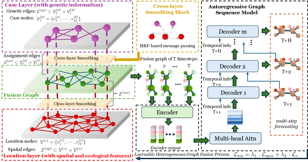
Figure 1: Framework of BLUE: BLUE consists of the following components: In Bi-layer Heterogeneous Graph Construction, we model avian influenza spread using a bi-layer heterogeneous graph that includes two types of nodes—infected cases and locations. Then, we apply an MRF-inspired Cross-layer Smoothing to reduce the impact of edge sparsity by aggregating information from neighbors. We simplify the heterogeneous graph into a single homogeneous Fusion Graph in Information-Preserving Fusion Graphs and retain the essential transmission structure through the spectral regularizer. Finally, Autoregressive Encoder–Decoder Forecasting encodes node interactions over a sequence of time and generates multi-step forecasts using an autoregressive decoder.

Bi-layer Heterogeneous Graph Construction.

Conventional GNN-based forecasting models simulate the spread of infectious diseases by constructing static transmission patterns that capture spatial and temporal dependencies among locations. However, these models provide only a single-view representation of spatial correlations and treat all infected cases as contributing equally to transmission intensity. As a result, they cannot distinguish between highly infectious cases and those with lower transmission potential. To address this limitation, we construct heterogeneous graphs that unify case-level infection intensity and location-level spatial connectivity within a single framework. These heterogeneous graphs incorporate both spatial (e.g.,geographical distance) and biological information (e.g., genetic similarities and host population abundance), with infection trends, allowing for more informative and dynamic representations. This unified approach supports multi-step spatio-temporal predictions that reflect both spatial and biological aspects.

Fig. 1 shows the architecture of heterogeneous graphs of one timestep. The node set $\mathcal{V}_{t}$ consists of two types of nodes: A fixed set of location nodes (red nodes) $\mathcal{V}^{(c)}=\{v^{(c)}_{1},\cdots,v^{(c)}_{N}\}$ with $N$ locations, each associated with a feature vector $\mathbf{x}_{i}^{(c)}(t)=[infected_{i}(t),population_{i}(t)]$, where $infected_{i}(t)$ is the number of newly reported infection cases in location $i$ at week $t$, and $population_{i}(t)$ is the bird abundance in location $i$ at week $t$. A time-varying set of case nodes (purple nodes) $\mathcal{V}^{(p)}_{t}=\{v^{(p)}_{1},\cdots,v^{(p)}_{M}\}$, each representing an individual infected sample reported at time $t$, with the feature vector $\mathbf{x}_{j}^{(p)}(t)$ encoding its genetic profile derived from pairwise genetic distances using the Kimura 2-parameter (K80) model on aligned hemagglutinin(HA) segment sequences (Kimura, 1980) (see Appendix C for details). The resulting distance matrix was row-normalized and projected into a fixed-size feature vector using spectral embedding, preserving the global genetic similarity structure.

The edge set $\mathcal{E}_{t}$ includes three types of edges: Assignment edges (purple and red dash lines), Genetic edges (purple lines), and Spatial edges (red lines). Assignment edges $\mathcal{E}^{(as)}\subset\mathcal{V}_{t}^{(p)}\times\mathcal{V}_{t}^{(t)}$ link each case to the location in which it was reported. These edges are binary. Genetic edges $\mathcal{E}^{(ge)}\subset\mathcal{V}_{t}^{(p)}\times\mathcal{V}_{t}^{(p)}$ connect genetically similar cases from biological modality, where each edge $\langle v_{k}^{(p)},v_{l}^{(p)}\rangle$ carries a similarity weight $w_{kl}^{(ge)}$ between case $k$ and case $l$. Spatial edges $\mathcal{E}^{(sp)}\subset\mathcal{V}^{(c)}\times\mathcal{V}^{(c)}$ connects spatially neighboring locations from geographical modality. Each edge $\langle v_{i}^{(c)},v_{j}^{(c)}\rangle$ is weighted by a geographic similarity score $\omega_{ij}^{sp}$ derived from inter-location distances. Empirical studies have shown that avian influenza (AI) outbreaks tend to exhibit highly localized spatial transmission patterns. In particular,  (Bonney et al., 2018) reports that the majority of lateral transmission occurs within a radius of approximately 30 km, with the probability of long-distance spread declining sharply beyond this range. To align with the observation, we employ a kernel-based edge weighting scheme that normalizes physical distances with a soft decay rather than applying a strict distance cutoff. For each undirected spatial edge between locations $i$ and $j$, we assign a weight using a Gaussian kernel:

$$\omega_{ij}^{sp}=K(D_{ij})=\exp\left(-\frac{D_{ij}^{2}}{2\sigma^{2}}\right)$$ (1)

where $D_{ij}$ is the geographic distance and $\sigma=\tau_{d}/3$, with $\tau_{d}=30$ km. This smooth decay function ensures that closer nodes have stronger connections, while links to distant locations are naturally suppressed without being abruptly removed, preserving meaningful local structure.

Formally, we consider the problem of forecasting the spread of avian influenza based on historical multi-source observations, structured as a sequence of dynamic, heterogeneous graphs. Let $\mathcal{G}_{t}=(\mathcal{V}_{t},\mathcal{E}_{t},\mathcal{T}_{V},\mathcal{T}_{E})$ denote a heterogeneous graph snapshot at week $t$, where $\mathcal{T}_{V}=\{\mathcal{V}^{(c)},\mathcal{V}^{(f)}\}$ and $\mathcal{T}_{E}=\{\mathcal{E}^{(sp)},\mathcal{E}^{(ge)},\mathcal{E}^{(as)}\}$ denote the sets of node and edge types respectively. Given a sequence of dynamic heterogeneous graphs over the past $T$ weeks, i.e., $\{\mathcal{G}_{1},\mathcal{G}_{2},\cdots,\mathcal{G}_{T}\}$, the spatial-temporal forecasting is to predict the number of new infections in each location for the subsequent $H$ weeks $\{\mathbf{y}_{T+1},\cdots,\mathbf{y}_{T+H}\}=f_{\theta}(\mathcal{G}_{1},\cdots,\mathcal{G}_{T})$, and our model aims to learn the function $f_{\theta}$ that maps the historical graph sequence to future case counts accordingly.

3.1 Cross-layer Smoothing Block

Avian influenza transmission involves complex interactions across cases and locations. Therefore, an effective strategy to aggregate and smooth feature representations across the case layer and location layer is essential for our heterogeneous graphs. We introduce the MRF-inspired cross-layer connection smoothing block to address the discrepancy of heterogeneous edges and nodes by explicitly leveraging local dependencies across heterogeneous graph neighborhoods, encouraging coherent representations within epidemiologically linked groups of nodes while preserving type-specific semantics.

The smoothing module leverages a mean-field approach that iteratively refines node embeddings on each heterogeneous graph. Formally, given an initial node embedding $x_{v}^{(0)}$ and three distinct edge types (spatial, genetic, and assignment edges), we perform $K$-time relation-specific message passing

$$m_{r}^{(k)}(v)=\frac{1}{|\mathcal{N}_{r}(v)|}\sum_{u\in\mathcal{N}_{r}(v)}W_{r}x_{u}^{(k-1)}$$ (2)

where $\mathcal{N}_{r}(v)$ denotes immediate neighbors of node $v$. $W_{r}$ is a trainable parameter matrix representing the strength of interactions between connected nodes under relation $r$, adhering to the local Markov property. These messages, reflecting smoothed neighbor information, are aggregated across relations and combined with a node type-specific bias $b_{\tau{(v)}}$:

$$x_{v}^{(k)}=\text{ReLU}(\sum_{r}m_{r}^{(k)}(v)+b_{\tau{(v)}})$$ (3)

Here, we employ a ReLU activation, ensuring each node embedding is influenced by its neighbors’ semantics. Iteratively applying this update $K$ times mimics multiple rounds of belief propagation, spreading information across the graph structure while explicitly considering different relational contexts. Thus, by restricting propagation to immediate neighbors, applying learnable, relation-specific transformations, and iteratively refining node representations, this approach effectively integrates key aspects of MRF inference into a differentiable graph-based learning framework.

3.2 Information-preserving Fusion Graphs

Heterogeneous graphs contain different types of nodes and relationships, making their structures inherently complex. This complexity arises from the simultaneous presence of diverse local and global relational dependencies. Converting heterogeneous graphs into a homogeneous form can significantly simplify representation; however, doing so typically risks losing valuable relational information from multiple sources. To overcome this limitation, we propose the Fusion Graph to transform the original heterogeneous structure, comprising location and case nodes connected by multiple relational types, into a unified one under spectral alignment (refers to Sec.  3.4 for details). Consequently, the Fusion Graph effectively captures the original heterogeneous complexity while providing a simpler and more interpretable structure (timestep $t$ is omitted for clarity).

Fusion Nodes.

Implementationally, we define fusion nodes as aggregated representations of locations, constructed by systematically integrating neighbor information from the original heterogeneous graph. Given an initial heterogeneous graph $\mathcal{G}_{t}$, fusion node embedding $\mathbf{x}_{i}$ corresponding to the location node $v_{i}^{(c)}\in\mathcal{V}^{(c)}$ at timestep $t$ is generated by

$$\mathbf{x}_{i}=f_{m}\left(f_{1}\left(\mathbf{x}_{i}^{(c)},\mathbf{x}_{i}^{(c\_spatial)}\right),\,f_{2}\left(\mathbf{x}_{i}^{(p)},\mathbf{x}_{i}^{p\_genetic}\right)\right)\in\mathbf{X}_{t}$$ (4)

where $\mathbf{x}_{i}^{(c)}$ and $\mathbf{x}_{i}^{(p)}$ are the features of the location and its associated cases, respectively. The term $\mathbf{x}_{i}^{(c\_spatial)}$ aggregates information from neighboring locations connected by spatial relationships, while $\mathbf{x}_{i}^{p\_genetic}$ summarizes genetic information derived from cases within the location. The specific aggregation functions, $f_{1}$ and $f_{2}$, and the subsequent fusion function $f_{(m)}$ employ Multi-Layer Perceptrons (MLPs) with nonlinear activation functions, effectively integrating diverse nodes into coherent fusion node embeddings.

Fusion Edges.

Once fusion node embeddings are obtained, we construct edges to induce a coherent relational topology. Instead of forcing every possible pair or using a hard cut-off, we employ a learnable link prediction network augmented with Locality-Sensitive Hashing (LSH) to select edges and ensure computational tractability. Specifically, for any pair of fusion nodes $v_{i}$ and $v_{j}$ (generated from location nodes $v_{i}^{(c)}$ and $v_{j}^{(c)}$), we define the link probability $p_{ij}$ as

$$p_{ij}=\sigma(W_{l}[\mathbf{x}_{i}\|\mathbf{x}_{j}]+b_{l})$$ (5)

with $\sigma(\cdot)$ is Sigmoid activation for normalization probabilities. $\|$ indicate vector concatenatnion, and $W_{l},b_{j}$ are learnable parameters. To avoid $O(N^{2})$ enumeration over all node pairs, we generate a reduced candidate set via LSH: node embeddings are projected onto $K$ random hyperplanes to produce binary codes, which approximate cosine similarity in the embedding space (Charikar, 2002). Specifically, each fusion node embedding $\mathbf{x}_{i}^{(f)}$ is converted into a $B$-bit binary code

$$\mathbf{h}_{i}=[\text{sign}(\mathbf{r}_{1}^{\top}\mathbf{x}_{i}),\cdots,\text{sign}(\mathbf{r}_{H}^{\top}\mathbf{x}_{i})]\in\{0,1\}^{B}$$ (6)

where $\mathbf{r}_{h}$ are independent random projection vectors sampled from a spherical distribution and $B$ is the length of binary codes. Nodes with identical hash codes are placed into the same group, and within-bucket pairs $(i,j)$ are considered candidate edges, leveraging the high collision probability of similar vectors. If the number of exact-match candidates is below a predefined maximum $M_{max}$, the candidate set is supplemented by selecting node pairs whose Hamming distance between codes does not exceed a threshold $\tau_{h}$=1. By grouping nodes via code matches, we avoid the cost of exhaustive pairwise comparison and reduce to approximately $O(N+M_{max})$ operations, where $N=|\mathcal{V}^{(c)}|+|\mathcal{V}^{(p)}_{t}|$ denotes the total number of location and case nodes at time $t$. We present the complexity details in Appendix A.

To integrate original heterogeneous relations into the fusion graph, BLUE further employs a gate network that dynamically weights spatial and genetic edges based on node-pair interactions. Formally, for each pair of fusion nodes $v_{i}$ and $v_{j}$, the relation-specific embedding

$$\mathbf{e}_{ij}^{(r)}=\mathbf{e}_{r}+\mathbf{W}_{edge}\mathbf{x}_{ij}^{(r)}+\mathbf{b}_{edge}$$ (7)

where $r\in\{spatial,genetic\}$, $\mathbf{e}_{r}$ is a learnable vector encoding relation type, and $\mathbf{x}_{ij}^{(r)}=\{\mathbf{x}_{i}^{(c)},\mathbf{x}_{j}^{(p)}\}$ contains the corresponding edge features. These embeddings are then fed into a multi-head self-attention network (Vaswani et al., 2017) to produce unnormalized scores and are normalized across relations

$$\mathbf{\alpha}_{ij}^{(r)}=\text{Attn}(\mathbf{x}_{i},\mathbf{x}_{j},\mathbf{e}_{ij}^{(r)}),\text{ }\mathbf{e}_{ij}^{(r)}=\sum_{r}\frac{\text{exp}(\mathbf{\alpha}_{ij}^{(r)})}{\sum_{r^{\prime}}\mathbf{\alpha}_{ij}^{(r^{\prime})}}\mathbf{e}_{ij}^{(r)}$$ (8)

The fusion-edge embedding is obtained as a weighted sum $\mathbf{e}_{ij}=\sum_{r}\alpha_{ij}^{(r)}\mathbf{e}_{ij}^{(r)}$. Thus, we obtain the unified fusion graphs, with updated fusion node embeddings and spatial distances and genetic correlations adaptively combined, enabling the model to emphasize the most informative relation for each node pair while preserving interpretability and end-to-end differentiability. To ensure the maximum information preservation during the fusion process, we employ a spectral regularizer to ensure the diffusion modes consistency (definition of the spectral regularizer in Sec. 3.4).

3.3 Autoregressive Encoder-Decoder Forecasting

To model temporal dynamics, we adopt a sequence-to-sequence architecture over the compressed fusion graphs. At each time step $t$ of the window size $T$, the fusion node embeddings $\mathbf{X}_{t}$ are propagated through $L$ GraphSAGE layers (Hamilton et al., 2017):

$$\mathbf{H}_{t}^{(l+1)}=\sigma(\text{GraphSAGE}_{l}(\mathbf{H}_{t}^{(l)},\mathbf{E}^{(f)}_{t}))\text{, for }l=0,1,\cdots,L-1\mathbf{H}_{t}^{(l+1)}=\sigma(\text{GraphSAGE}_{l}(\mathbf{H}_{t}^{(l)},\mathbf{E}^{(f)}_{t}))\text{, for }l=0,1,\cdots,L-1$$ (9)

where $\mathbf{H}_{t}^{(0)}=[\mathbf{X}_{t}+\mathbf{p}_{t}]$, $\mathbf{p}_{t}$ denotes learnable positional encoding. $\mathbf{E}^{(f)}_{t}=\{\mathbf{e}_{ij}\}$ is the edge embeddings of the fusion graph at timestep $t$. Over $T$ observations, we collect the final-layer outputs of each timestep $\{\mathbf{H}_{t}^{(L)},\cdots,\mathbf{H}_{t+w-1}^{(L)}\}$ and stack them into $\mathcal{H}\in\mathbb{R}^{w\times N\times d}$. This tensor is fed into a temporal-aware fusion module, implemented by the multi-head attention network (Vaswani et al., 2017), to enforce features mutually concern across steps, capturing temporal dependence and yielding a context vector $\mathbf{H}^{(c)}$. Following, the decoder operates in an autoregressive manner over a forecasting horizon of length $H$. At each step $h\in\{1,\cdots,H\}$, it applies a GraphSAGE-based architecture composed of $L$ layers that mirror the encoder structure:

$$\mathbf{d}_{h}\leftarrow\left\{\begin{aligned} &\text{Decoder}(\mathbf{Z}_{h-1}^{(L)},\mathbf{E}_{T}^{(f)},\mathbf{f}_{h-1},\mathbf{t}_{h})\text{, when }h\geq 1\\ &\text{Decoder}(\mathbf{H}^{(c)},\mathbf{E}_{T}^{(f)},\mathbf{f}_{h-1},\mathbf{t}_{h})\text{, when }h=0\end{aligned}\right.$$ (10)

Here, $\mathbf{Z}_{h-1}^{(L)}$ denotes the hidden state from the previous decoding step, $\mathbf{E}^{(f)}_{T}$ represents the fusion edge embeddings at the final observation time $T$, and $\mathbf{t}_{h}$ encodes temporal information. The decoded features $\mathbf{d}_{h}$ are then smoothly integrated with with the previous step’s decoded output $\mathbf{f}_{h-1}$ and the encoder’s global context representation $\mathbf{H}^{(c)}$ through a weighted combination:

$$\tilde{\mathbf{d}}_{h}=(1-\lambda_{o}-\lambda_{p})\mathbf{d}_{h}+\lambda_{o}\mathbf{f}_{h-1}+\lambda_{p}\mathbf{H}^{(c)}$$ (11)

where $\lambda_{o},\lambda_{p}\in[0,1]$ control the reliance on current decoding, prior predictions, and global context, respectively, enhancing forecast stability across longer horizons. Finally, the prediction for step $h$, denoted as $\hat{\mathbf{y}}_{h}$, is generated via a nonlinear projection $\hat{y}_{h}=\mathbf{W}_{out}\tilde{\mathbf{d}}_{h}$. The hidden state for the current step is updated by a linear combination of $\tilde{\mathbf{d}}_{h}$ and the prior hidden states, enabling information flow across steps during sequential prediction.

3.4 Optimization

During training, BLUE minimizes a composite objective that couples (i) multi-step forecasting term, (ii) spectral alignment of the learned fusion graph, and (iii) standard parameter regularization. Firstly, the forecasting term $\mathcal{L}_{\mathrm{pred}}=\frac{1}{N\,H}\sum_{h=T+1}^{T+H}\sum_{i=1}^{N}\bigl{(}\hat{y}_{i,h}-y_{i,h}\bigr{)}^{2}$ measures the mean-squared error (MSE) between the forecast $\hat{y}_{i,h}$ and the ground-truth infection count $y_{i,h}$ across prediction horizon. Secondly, compressing heterogeneous graphs into homogeneous ones is a spectral low-pass filter: high-frequency components that live on the fine, case-level sub-graph are discarded. Consequently, operating only on the fused graph risks under-representing subtle transmission channels driven by a few genetically distinctive samples. Spectral regularize $\mathcal{L}_{\mathrm{spec}}=\bigl{\|}\,\mathbf{L}_{hetero}-\mathbf{L}_{f}\bigr{\|}_{F}^{2}$ works as an information-preserving constraint to match the spectrum between the original heterogeneous graphs and compressed ones. $\mathbf{L}_{hetero}=\mathbf{D}_{hetero}-\mathbf{A}_{hetero}$ is the Laplacian of original heterogenous graphs. $\mathbf{D}_{hetero}=diag(\mathbf{A}_{hetero}\mathbf{1})$ and $\mathbf{A}_{hetero}$ is the adjacency matrix of heterogeneous graphs driven from link-predictor probabilities $\mathbf{\omega}^{sp}$. $\mathbf{L}_{f}=\mathbf{D}_{f}-\mathbf{A}_{f}$ is the fusion Laplacian, with $\mathbf{A}_{f}$ the adjacency matrix of fusion graphs. It compels the Laplacian of the learned fusion graph to approximate, in a spectral sense, the Laplacian of the original heterogeneous graph. Collaborating with GraphSAGE layers based on random walk, it keeps the large-scale diffusion geometry of the data intact even after the graph has been aggressively compressed (details in Appendix B). Finally, the overall objective is formed, with $\lambda_{1},\lambda_{2}$ controlling the weights of spectral alignment and regularization

$$\mathcal{L}_{\mathrm{tot}}\;=\;\underbrace{\frac{1}{N\,H}\sum_{h=T+1}^{T+H}\sum_{i=1}^{N}\bigl{(}\hat{y}_{i,h}-y_{i,h}\bigr{)}^{2}}_{\mathcal{L}_{\mathrm{pred}}}\;+\;\lambda_{\mathrm{1}}\,\cdot\underbrace{\bigl{\|}\,\mathbf{L}_{hetero}-\mathbf{L}_{f}\bigr{\|}_{F}^{2}}_{\mathcal{L}_{\mathrm{spec}}}\;+\;\lambda_{2}\,\underbrace{\sum_{w\in\Theta}\|w\|_{2}^{2}}_{\mathcal{L}_{r}}$$ (12)

4 Experiments

We evaluate BLUE on two infection-forecasting datasets: (1) The Flu-Japan dataset, collected from the Infectious Diseases Weekly Report (IDWR) , comprises weekly influenza-like illness counts from 47 prefectures in Japan over the period 2012–2019. We utilized this dataset introduced by (Deng et al., 2020). Its adjacency matrix is binary, indicating whether the geodesic distance between any two prefectures exceeds a predefined cutoff. (2) Our Avian-US, constructed as described in Appendix C, covers 3,227 counties and integrates three complementary modalities: 1) Genetic: pairwise similarity scores among cases within and across counties; 2) Geographic: inter-location distances, 3) Ecological: local bird species abundance metrics. Combining two real-world datasets, we aim to demonstrate BLUE’s capacity to leverage heterogeneous relational information for accurate, early-warning forecasts.

Baselines.

We compare BLUE against two categories of GNN-based models: 1) general spatio-temporal forecasting models, including ST-GCN (Yu et al., 2018), SelfAttnRNN (Cheng et al., 2016), DCRNN (Li et al., 2018), and EAST-Net (with a simplify version ST-Net) (Wang et al., 2022b), and epidemic prediction model: Cola-GNN (Deng et al., 2020), EpiGNN (Xie et al., 2022), Epi-cola-GNN (Liu et al., 2023b). The baseline models are primarily designed for single-layer spatio-temporal forecasting and assume either a fixed or learnable graph structure. As such, they are not directly compatible with the multi-layer architecture of the Avian-US dataset. To make them applicable, we adapt each model by building homogeneous graphs tailored to its design. For ST-GCN, SelfAttnRNN, Cola-GNN, EpiGNN, EpiCola-GNN, and DCRNN, we define a binary adjacency matrix based on spatial proximity between counties. This setup mirrors their original use cases, allowing these models to learn spatio-temporal patterns over a fixed location-level graph. For ST-Net and EAST-Net, which support adaptive graph learning, we initialize homogeneous graphs with no predefined edges. These models learn the graph structure dynamically, allowing them to infer inter-location dependencies during training without relying on geographic priors.

Experimental settings.

To comprehensively evaluate the performance of the proposed method and baseline models, we adopt four complementary metrics: Root Mean Squared Error (RMSE), Mean Absolute Error (MAE), Pearson Correlation Coefficient (PCC), and F1 Score (F1). RMSE and MAE quantify the absolute and squared deviations between predicted and ground-truth counts. PCC measures the linear correlation between predicted and observed infection trends across spatial and temporal dimensions. F1 Score evaluates binary outbreak detection performance. To reflect this, we set a short observation window of $T$=4 steps and forecast the next $H$=4 steps (all experiments are conducted under this setting unless specified), and report the averaged evaluation metrics of $H$ steps. Experiments of all baselines and BLUE are conducted under a 5-fold cross-validation with the same random seed to ensure consistency. In addition to fixed embedding size $d$=8 and weight regularization $\lambda_{2}=5e-4$, all baseline models are re-trained and tuned for optimal performance using their official open-source code (see Appendix D). For BLUE, we search $\lambda_{1}\in\{0.01,0.05,0.1,0.5,1\}$, and choose $\lambda_{1}=0.1$ for final evaluations. (The final set of all parameters is listed in the supplementary D). All experiments are run on either a single NVIDIA V100, DGX A100, or NVIDIA RTX A5000 GPU.

Table 1: Overall performance on Flu-Japan (up) and Avian-US (down) dataset. Experiments are run under window size $T$=4 and prediction horizon $H$=4, with 5-fold validation. $\uparrow,\downarrow$ indicate the preferred direction. Best results are bolded. Runner-up baseline results are underlined.

Dataset	Flu-Japan
model	STGCN	SelfAttnRNN	ST-Net	EAST-Net	DRCNN	EpiGNN	Cola-GNN	Epi-Cola-GNN	BLUE
RMSE($\downarrow$)	1763±764	1730±782	1761±727	1723±790	1789±788	1742±707	1600±765	1631±787	1511±331
MAE($\downarrow$)	995±726	876±760	1083±893	1038±848	1216±1084	896±721	886±758	1368±1124	553±150
PCC($\uparrow$)	07316±0.0794	0.7850±0.0562	0.7898±0.0923	0.7352±0.0573	0.7674±0.0582	0.7401±0.0778	0.7135±0.1054	0.7486±0.0784	0.7954±0.0328
F1($\uparrow$)	0.6551±0.2437	0.7040±0.2840	0.7171±0.2563	0.6398±0.6637	0.6663±0.2491	0.6699±0.2388	0.6747±0.2472	0.6831±0.2793	0.7234±0.2420

Dataset	Avian-US
model	STGCN	SelfAttnRNN	ST-Net	EAST-Net	DRCNN	EpiGNN	Cola-GNN	Epi-Cola-GNN	BLUE
RMSE($\downarrow$)	1.6141±0.2435	1.6467±0.2386	1.6840±0.2598	1.6333±0.2424	1.1284±0.2339	0.7727±0.1201	0.7222±0.1110	0.6963±0.1009	0.6255±0.1096
MAE($\downarrow$)	1.1954±0.1389	1.4200±0.1895	1.1282±0.1405	1.1490±0.1331	1.1177±0.1400	0.7139±0.1247	0.0916±0.1123	0.0987±0.1097	0.0549±0.1121
PCC($\uparrow$)	0.0086±0.0006	0.0092±0.0005	0.0057±0.0003	0.0051±0.0003	0.0097±0.0006	0.0094±0.0010	0.0053±0.0005	0.0078±0.0008	0.0074±0.0011
F1($\uparrow$)	0.0145±0.0114	0.0172±0.0109	0.0245±0.0173	0.0261±0.0110	0.0221±0.0136	0.0223±0.0150	0.0232±0.0106	0.0262±0.0110	0.0268±0.0122

4.1 Overall Performance

Flu-Japan dataset.

As shown in Table 1, BLUE achieves the lowest RMSE and MAE in Flu-Japan, indicating high accuracy in case count prediction and stable performance across folds, with lower standard deviations than other models. All methods show high variability, which is likely driven by the uneven distribution of cases, especially since the Flu-Japan dataset includes extreme outbreaks in some folds while other folds are relatively stable, influencing the fold-level statistics. BLUE achieves a higher PCC of 0.7954 with reduced variance, showing its robustness in capturing non-local transmission lags and recurring patterns compared to GRU- and CNN-based alternatives. It consistently ranks highest in F1 score and simultaneously lowers MAE, indicating that it reduces false alarms in low-incidence prefectures without missing outbreaks in high-incidence ones.

Avian-US dataset.

In the Avian-US dataset, DRCNN achieves the highest PCC. However, PCC is sensitive to small fluctuations, especially in a sparse dataset like Avian-US, and can be skewed by regions with few or no cases. Since PCC only measures linear correlation, it does not fully reflect the model’s effectiveness in capturing the true outbreak dynamics. On more robust metrics, BLUE shows a clear advantage: it reduces RMSE and MSE by 0.0708 and 0.0438, respectively, compared to the runner-up (EpiCola-GNN). It also exhibits lower standard deviation across cross-validation folds, demonstrating its stability and consistency for infection count prediction. BLUE achieves the highest F1 score, which better captures the model’s ability to detect infection occurrences rather than precise case counts, indicating its high effectiveness in outbreak detection. (Model performance under varying observation window sizes $T$ and prediction horizons $H$ is provided in Appendix E.)

4.2 Ablation Study

Ablation studies are conducted on the Avian-US dataset to evaluate the contributions of each part in BLUE. We introduce 4 variants: 1) w/o CS excludes the cross-layer smoothing block from BLUE; 2) w/o gen only utilizes the spatial distances and assignment relationships; 1) w/o CS+gen only implement the auto-regressive encoder-decoder framework; 4) w/o Spec excludes the spectral terms from the objective function. The results are shown in Table. 3. Disabling the CS module leads to a significant increase in RMSE, from 0.6255 to 1.5230, and results in a huge drop in accuracy. Without CS, the graph messages become noisy due to the sparsity and discrepancy of the initial heterogeneous edges. The MRF refinement introduced by CS plays a clear role in filtering out this noise and generating cleaner embeddings that support more accurate decoding. Removing genetic edges results in an even greater increase in MAE than removing CS alone, indicating that spatial graphs by themselves cannot fully capture cross-location outbreak patterns of avian influenza. The performance further drops when both CS and genetic edges are removed, suggesting a mutual information between the two components: CS spreads epidemiologically meaningful signals across the graph, while genetic edges determine which signals are epidemiologically relevant. Without the spectral alignment constraint, the link predictor tends to overfit, resulting in a significant decrease in predictive performance, indicating the connectivity structure no longer aligns with the underlying epidemiological diffusion process. BLUE achieves the best performance, demonstrating the contributions of every component.

Table 2: Ablation study on Avian-US.

Variants	RMSE	MAE	F1	PCC
w/o CS	1.5230	1.1295	0.0117	0.0030
w/o gen	1.7112	1.6530	0.0161	0.0054
w/o CS+gen	2.4290	2.0560	0.0030	0.0021
w/o Spec	2.9998	2.9191	0.0014	0.0017
BLUE	0.6255	0.1549	0.0268	0.0074

Table 3: Impact of $\lambda_{1}$

$\lambda_{1}$	RMSE	MAE	F1	PCC
1	0.7143	0.2935	0.0023	0.0157
0.5	0.6301	0.0617	0.0029	0.0257
0.1	0.6255	0.0549	0.0074	0.0268
0.05	0.6296	0.0566	0.0044	0.0263
0.01	0.6312	0.0911	0.0021	0.0287

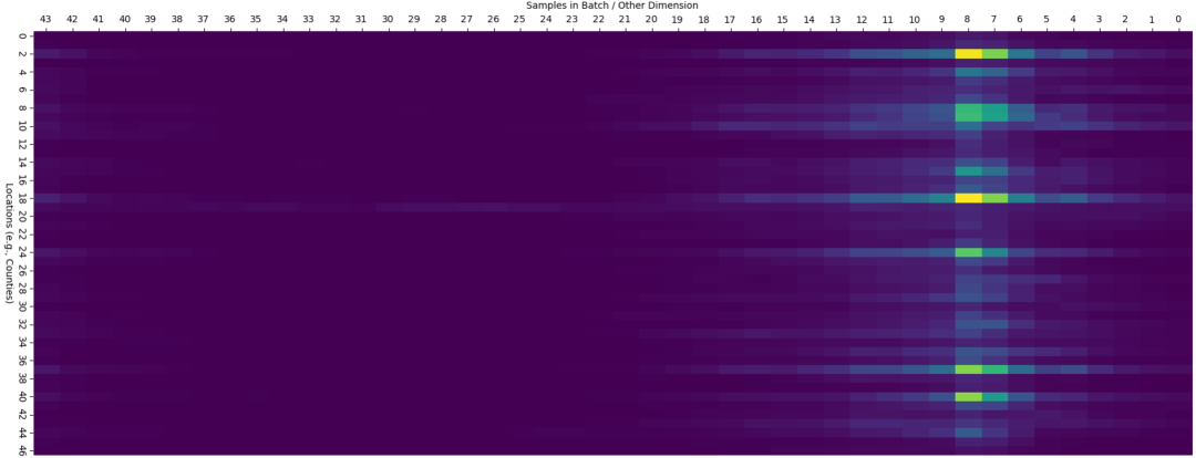
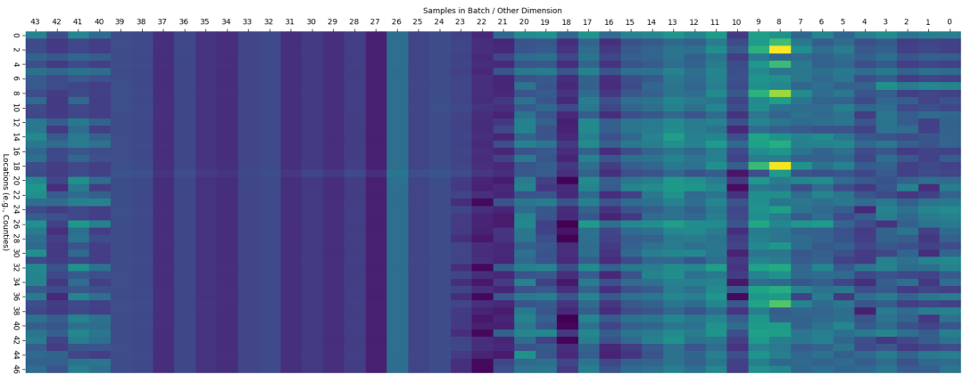
Figure 2: Heatmap of ground truth (left) and prediction (right) on Flu-Japan dataset.

4.3 Spectral Alignment $\mathcal{L}_{spec}$

The spectral alignment term $\mathcal{L}_{spec}$ guarantees the alignment of the heterogeneous information between the original bi-layer heterogeneous graphs and fusion graphs. As shown in Table. 3, As $\lambda_{1}$ decreases, most evaluation metrics show a pattern of initial improvement followed by degradation. For example, RMSE decreases from 0.6301 to 0.6255 and rises again once the weight falls to 0.01. We observed that the prediction loss $\mathcal{L}_{pred}$ is much smaller and the spectral alignment loss is larger on the Avian-US dataset. Using a large $\lambda_{1}$ enforces the model to over-prioritize the spectral alignment, underfitting the actual prediction tasks and resulting in suboptimal forecasting results.

4.4 Case study on Flu-Japan dataset

We provide the heatmap of experimental results on the Flu-Japan dataset, shown in Fig. 2. Both the ground truth and predicted heatmaps exhibit a distinct peak in activity during the 8th batch. BLUE not only identifies this peak at the correct temporal position but also accurately reproduces its spatial distribution across multiple prefectures, demonstrating that the model has effectively learned both the timing and spatial structure of the outbreak. In the ground truth heatmap, bright horizontal bands correspond to a small subset of highly infected prefectures. BLUE’s predictions highlight these same regions while maintaining low activity for the remaining prefectures, indicating that the model captures the dominant transmission pathways without overpredicting infection spread.

5 Conclusion and Discussion

We present BLUE, a bi-layer heterogeneous graph fusion network that integrates genetic and spatial data to improve epidemic forecasting. BLUE uses cross-layer smoothing and information-preserving graph fusion to learn coherent representations of disease spread through an autoregressive encoder–decoder architecture. We evaluate BLUE on two datasets: the newly constructed Avian-US dataset and the publicly available Flu-Japan dataset. In both settings, BLUE outperforms strong spatio-temporal and epidemic forecasting baselines, demonstrating its effectiveness across different spatial and epidemiological contexts. The spectral fusion mechanism within BLUE is generalizable and can be extended to maintain structural alignment in more complex, multi-layer graph settings. While the current version of the Avian-US dataset does not include environmental variables, the architecture of BLUE is inherently modular and extensible. Additional information, such as location-level temperature, humidity, or other ecological indicators, can be incorporated as new layers or features with corresponding cross-layer connections. In future work, we plan to expand the dataset with richer environmental attributes and biological categories, such as mammals and humans, to better support realistic forecasting, extending BLUE’s applicability to more comprehensive, real-world scenarios.

6 Acknowledgment

This research is supported by the ARC Center of Excellence for Automated Decision Making and Society (CE200100005). We acknowledge the utilization of computational resources from the Katana High Performance Computing (HPC) cluster, which is supported by the Faculty of Science, UNSW Sydney. We also acknowledge the National Computational Infrastructure (NCI) for providing access to the Gadi supercomputer.

Appendix A Local Sensitive Hashing Complexity

Code Construction.

For each bi-layer heterogeneous graph, the total number of location nodes is $N=|\mathcal{V}^{(c)}|+|\mathcal{V}^{(p)}_{t}|$. The length of each binary code for the Local Sensitive Hashing sampler is denoted as $B$. To generate LSH codes, we take $B$ dot products between node embeddings (with dimension $d$) and independently sampled random hyperplanes $\mathbf{r}_{b}$, retaining only the sign of each projection and resulting in a per-node cost of $O(Nd)$ for computing projections and $O(B)$ for extracting sign bits. Across all $N$ nodes, the overall cost is $O(NBd)$, primarily from matrix-vector multiplications. Once the LSH codes are computed, each node is inserted into a hash map using its binary signal as the key, adding a total $O(N)$ time cost for the hash table construction. The complete time complexity for code generation and hashing is thus $O(NBd+N)$.

Bucket Matching.

Each bucket with $k$ nodes encodes $\frac{k(k-1)}{2}$ potential node pairs. The LSH-based sampler terminates when the number of collected node pairs reaches the limit of $M_{max}$, ensuring this step remains within $O(M_{max})$ time.

If additional pairs are needed, we perform the following strategy: With randomly selected nodes, we search their neighbors within the Hamming distance threshold $\tau_{h}=1$. Since the number of selected nodes and their neighbors are constants, the computation takes $O(B)$ in total.

Combining all terms gives:

$$T_{total}=O(NBd+N+M_{max}+B)$$ (13)

Since the embedding size $d$ and code length $B$ are fixed constants in implementation, the complexity simplifies to $O(N+M_{max})$, highlighting the scalability of our LSH-based sampler compared to naive pairwise similarity joins, which require $O(N^{2})$ pairwise operations.

In practice, we replace the hash table implementation with a sorting-based alternative. Specifically, each node’s $B$-bit binary code is converted into a single integer representation in $O(NB)$ time. The resulting integer codes are then sorted in $O(N\log N)$ time. Although the total time complexity of this sorting-based LSH variant becomes $O(N\log N+M_{max})$, which is asymptotically higher than the hash map-based approach, it is empirically faster on GPU architectures due to the inefficiency of hash table operations in parallel settings.

Appendix B Spectral Approximation

Let $P\in\{0,1\}^{(N+M_{max})\times N}$ be the projection that aggregates case nodes into their home locations. $\mathbf{A}_{hetero}$ and $\mathbf{L}_{hetero}$ be the layer-adjacency and Laplacian of the heterogenous graph, and let $\mathbf{A}_{f}$ and $\mathbf{L}_{f}$ be the learned fusion-graph adjacency and Laplacian of the learned fusion graph. We can view fusion as a Spectral Approximation. Standard results in (Spielman and Teng, 2011) show that if the Laplacians satisfy

$$\|\mathbf{L}_{hetero}-\mathbf{L}_{f}\|_{2}\leq\varepsilon\|\mathbf{L}_{hetero}\|_{2},\varepsilon\ll 1$$ (14)

then the spectral properties of $\mathbf{A}_{hetero}$ and $\mathbf{A}_{f}$, e.g., eigenvalues and eigenvectors, differ by at most $O(\varepsilon)$. In particular, their adjacencies obey

$$\|\mathbf{A}_{hetero}-P\mathbf{A}_{f}P^{\top}\|\leq\varepsilon\|\mathbf{A}_{hetero}\|_{2}$$ (15)

Under this guarantee, any polynomial graph filter $p(\cdot)$ with Lipschitz constant $L_{p}$ is approximated by $Pp(\mathbf{A}_{f})P^{\top}$ up to a factor $O(\varepsilon)$

$$\|p(\mathbf{A}_{hetero})-Pp(\mathbf{A}_{f})P^{\top}\|\leq\mathbf{L}_{p}\varepsilon\|\mathbf{A}_{hetero}\|_{2}$$ (16)

Thus, any GNN layer executed on the fusion graph approximates the same layer on the original heterogeneous graph within a provably bounded $O(\varepsilon)$ error.

Let $\mathcal{F}_{hetero}(\mathbf{X})=p(\mathbf{A}_{hetero})\mathbf{X}$ and $\mathcal{F}_{f}(P^{\top}\mathbf{X})=Pp(\mathbf{A}_{f})P^{\top}\mathbf{X}$ denote the complete pipelines defined on the heterogeneous and fusion graphs, respectively. We implement GNNs with a stack of $L$ GraphSAGE layers in BLUE, where each layer operates as follows:

$$\sigma(\text{GraphSAGE}_{l}(\mathbf{H}_{t}^{(l)},\mathbf{E}^{(f)}_{t}))=\sigma(\mathbf{W}_{s}\mathbf{H}_{t}^{(l)}+\mathbf{W}_{n}\mathbf{D}^{-1}\mathbf{A}_{f}\mathbf{\mathbf{H}}_{t}^{(l)})$$ (17)

Here, $\sigma$ is ReLU activation. $\mathbf{A}_{f}$ is the adjacency matrix constructed from fusion edges $\mathbf{E}^{(f)}_{t}$, and $\mathbf{D}$ is its corresponding degree matrix. The polynomial GraphSAGE filter $p(\cdot)=\mathbf{D}^{-1}\mathbf{A}_{f}$ has spectral norm at most 1, and the ReLU activation is 1-Lipschitz. Thus, each GraphSAGE layer is $Z$-Lipschitz with $Z\leq\|\mathbf{W}_{s}\|_{2}+\|\mathbf{W}_{n}\|_{2}$, which implies that the per-layer discrepancy is bounded by $Z\|\mathbf{A}_{hetero}\|_{2}$. After stacking $L$ GraphSAGE layers, the cumulative error discrepancy is amplified by a factor of $\frac{Z^{L}-1}{Z-1}$. Hence for any input features $\mathbf{X}$, the overall discrepancy satisfies

$$\|\mathcal{F}_{hetero}(\mathbf{X})-\mathcal{F}_{f}(P^{\top}\mathbf{X})\|\leq\frac{Z^{L}-1}{Z-1}\|p(\mathbf{A}_{hetero})-Pp(\mathbf{A}_{f})P^{\top}\|\|\mathbf{X}\|=O(\frac{Z^{L}-1}{Z-1}\varepsilon)\|\mathbf{X}\|$$ (18)

where $\varepsilon=\|p(\mathbf{A}_{hetero})-Pp(\mathbf{A}_{f})P^{\top}\|=\|\mathbf{L}_{hetero}-\mathbf{L}_{f}\|_{2}$ captures the spectral difference between the heterogeneous and fusion graph Laplacians. By regularizing this spectral discrepancy, we ensure that the fusion graph preserves the dominant diffusion modes of the original heterogeneous structure. Consequently, downstream GNN computations and multi-step forecasts remain within an $O(\varepsilon)$ neighborhood of the predictions obtained on the full heterogeneous graph.

In our implementation, rather than enforcing strict equality between the Laplacians of the fusion graph and the original heterogeneous graph, we focus on preserving the most structurally informative components of the spectrum. Specifically, we constrain the largest $k$ eigenvalues of two graphs, which capture the global structures of the graph. By aligning the leading eigenvalues, we ensure that the fusion graph retains the essential global topology of the original heterogeneous graph and reduces sensitivity to discrepancies in the high-frequency components, which are often associated with local noise or unstable high-resolution variations. Consequently, the spectral loss remains robust and less prone to overfitting to noisy graph details.

Appendix C Avian-US Dataset

Table 4: Dataset statistics.

dataset	size (# locations $\times$ # week)	Min	Max	zeros (%)
FLU-Japan	47 $\times$ 348	0	26635	15.8
Avian-US	3227 $\times$ 104	0	92	98.4

The Avian-US dataset is a spatiotemporal, multi-modal dataset designed to support forecasting and modeling of avian influenza outbreaks across the United States. It integrates epidemiological records, viral genomic sequences, and host population data across 3,227 U.S. counties from 2021–2024. Each modality is spatially and temporally aligned at the county-week level, enabling multi-layered graph construction for downstream forecasting tasks.

C.1 Data Collection

This dataset integrates spatiotemporal outbreak data, genomic sequences, and species-level abundance observations into a structured multilayer representation for disease forecasting. Each stream was independently collected but programmatically harmonized for modeling integration.

Infected case data were sourced from federal surveillance systems and include time-stamped infection reports for host data recorded at the county level across the continental United States from 2021 to 2024. Each record includes a free-text host descriptor, location metadata, and a collection date. To standardize taxonomic information, host descriptors were programmatically mapped to a reference taxonomy using a hierarchical classification schema derived from the International Ornithological Congress (IOC) avian taxonomy. This resolved inconsistencies such as overlapping or ambiguous common names by aligning to stable scientific identifiers.

Genomic data consist of hemagglutinin (HA) segment sequences found in publicly available viral genome repositories for Biotechnology Information (NCBI). Sequences with sufficient metadata were retained and filtered to include only wild bird hosts. A probabilistic record linkage model was used to associate sequences with case records. This model was trained on labelled match/non-match examples and used gradient-boosted decision trees to compute a match score based on taxonomic agreement, spatial proximity, and temporal overlap (within a ±14-day window). High-confidence matches were retained for downstream analysis.

Host population data were drawn from the eBird Status and Trends product, which provides weekly abundance estimates at  3 km resolution for North American bird species eBird (2022). Raster values were extracted for each species and week, then aggregated at the county level to align with the spatial granularity of case data. Only wild bird species were retained, and abundance vectors were indexed by county and week.

All records were assigned stable identifiers and organized into structured, timestamped tables. The pipeline ensures consistency across modalities while maintaining temporal fidelity and species-level resolution.

C.2 Data Description

The dataset comprises real-world, multi-source data documenting avian influenza outbreaks in the United States from January 2021 to December 2024. It includes temporally aligned information on confirmed infection cases, viral genome sequences, and wild bird abundance estimates, collected and harmonized at a weekly resolution.

The epidemiological component consists of over 12,000 reported H5-positive wild bird cases, spanning all 48 contiguous U.S. states. Each record includes collection date, geographic location (mapped to U.S. counties), and host classification. Taxonomic labels were normalised using a hierarchical mapping system that resolves ambiguous or underspecified entries to consistent species-level identifiers, informed by IOC naming conventions.

A subset of 8,000 cases was associated with full or partial HA segment sequences retrieved from public repositories. Genomic data were filtered to retain wild bird hosts only, and sequence metadata (host, date, location) were cleaned and harmonised to match epidemiological records. Genomic divergence between HA segment sequences was computed using the K80 model, which accounts for substitution asymmetry between transitions (A$\leftrightarrow$G, C$\leftrightarrow$T) and transversions. For each aligned sequence pair, we calculate the observed proportions of transitions ($P$) and transversions ($Q$), and estimate the evolutionary distance $d$ as:

$$d=-\tfrac{1}{2}\log(1-2P-Q)-\tfrac{1}{4}\log(1-2Q)$$

where $P=\frac{\#\text{transitions}}{L}$ and $Q=\frac{\#\text{transversions}}{L}$, with $L$ denoting the aligned sequence length. This evolutionary distance matrix encodes biologically grounded measures of divergence under a continuous-time Markov model and is well-suited for comparing within-clade avian influenza sequences. It is used as an input feature for constructing genomic similarity edges in the downstream heterogeneous graph.

Host population context was derived from over 630 weekly avian abundance layers produced by the eBird Status and Trends project eBird (2022). These layers estimate relative abundance of bird species at  3 km resolution across North America. Raster values were extracted and aggregated at the county level for all species matching wild bird families in the outbreak dataset. The resulting abundance vectors were aligned weekly to match case timelines and stored in compressed array format.

All data layers were temporally aligned by epidemiological week. Metadata were standardised across data types, with fields for date, location, taxonomic label, and abundance scores. Unique identifiers were assigned to all records to enable traceability across modalities. The dataset is designed to support temporal, ecological, and genetic analysis of avian influenza dynamics in wild bird populations using real-world observations, without reliance on synthetic or simulated data.

Appendix D Implementation details

In our empirical evaluations, we implement ST-GCN, SelfAttnRNN, DCRNN, and Cola-GNN using the open-source Cola-GNN repository . ST-Net and EAST-Net are built upon the official EAST-Net implementation . Implementation of Epi-GNN  and Epi-Cola-GNN  are based on their respective publicly available source code.

To enable evaluation of the proposed BLUE framework on the Flu-Japan dataset, we first construct the location layer based on the provided adjacency matrix. Each location node is assigned features based on the reported infection counts across prefectures. To represent case-level information, we simulate case nodes and associate them with their respective infected locations. Unlike the Avian-US setting, we assume uniform infectivity and assign an equal importance feature (value = 1) to each case node. This simplifies the transmission model by treating all cases as equally influential. With this setup, we construct the heterogeneous graphs for the Flu-Japan dataset and use feed them into BLUE under the same modeling assumptions used in the Avian-US dataset.

To ensure comparability in overall performance, we unify the embedding size and hidden dimensions across all models and re-run each baseline on both datasets. The key hyperparameters used for all baseline models are listed below:

ST-GCN: embedding size=8, hidden dim=16, number of layers=3, epoch=100, learning rate=1e-5, dropout=0.3, window size=4, predicted horizon=4, weight of regularization term=5e-4.

SelfAttnRNN: embedding size=8, hidden dim=16, number of layers=2, epoch=100, learning rate=1e-5, dropout=0.3, window size=4, predicted horizon=4, weight of regularization term=5e-4.

DCRNN: embedding size=8, hidden dim=16, number of layers=2, max step of random walk=3, epoch=100, learning rate=1e-5, dropout=0.3, window size=4, predicted horizon=4, weight of regularization term=5e-4.

Cola-GNN: embedding size=8, hidden dim=16, number of filter=10, dilated rate for short term=1, dilated rate for long term=2, epoch=100, learning rate=1e-5, dropout=0.3, number of RNN layers=1, number of GNN layers=2, window size=4, predicted horizon=4, weight of regularization term=5e-4.

ST-Net: embedding size=8 (data) and 8 (time), Chebyshev layers=3, encoder layer=2, decoder layer=2, epoch=100, learning rate=1e-5, dropout=0.3, window size=4, predicted horizon=4, weight of regularization term=5e-4.

EAST-Net: spatial embedding size=8, modality embedding size =4, time embedding size=8, mobility prototype number = 8, memory dimension = 16, Chebyshev layers=3, encoder layer=2, decoder layer=2, epoch=100, learning rate=1e-5, dropout=0.3, window size=4, predicted horizon=4, weight of regularization term=5e-4.

Epi-GNN: embedding size=8, hidden dim=16, hidden dim of attention layer=64, pooling layer=2, patience=100, GNN layers=2, filer size=$\mathbf{f}_{1\times 5,1}$ and $\mathbf{f}_{1\times 3,1}$, window size=4, predicted horizon=4, epoch=100, learning rate=1e-5, dropout=0.3, weight of regularization term=5e-4.

Epi-Cola-GNN: embedding size=8, hidden dim=16, weight of epidemiological loss=0.5, patience=150, epoch=100, learning rate=1e-5, dropout=0.3, window size=4, predicted horizon=4, weight of regularization term=5e-4.

BLUE: embedding size=8, construction smoothing layer $K$=3, $B$=10, GraphSAGE layers $L$=2, $\lambda_{1}$=0.1, $\lambda_{2}$=5e-4, epoch=100, learning rate=1e-5, dropout=0.3, window size=4, predicted horizon=4. For Avian-US dataset, we set $\lambda_{o}$=0.1 and $\lambda_{p}$=0.3. For Flu-Japan dataset, we set $\lambda_{o}$=0.2, $\lambda_{p}$=0.3.

To manage data sparsity and numerical variation, we use four normalization techniques for preprocessing all feature data:

1. Min-Max Normalization: $x_{normalized}=(x-min)/(max-min)$. This method preserves value relationships but is sensitive to outliers.

2. Z-Score Normalization: $x_{normalized}=(x-mean)/std$. Suitable for approximately normally distributed features, it offers improved robustness to outliers compared to Min-Max scaling.

3. Log-MinMax Normalization: Applies a log transformation $log(x+\delta)$ followed by Min-Max scaling. This is effective for highly skewed positive-valued features with wide dynamic ranges.

4. Log-Plus-One Normalization: $log(x+1)$. This transformation is appropriate for heavily skewed count data with many zeros, as it maintains the presence of zero values.

Log-based normalization is particularly effective for exponentially distributed features or datasets with a high proportion of zeros. Accordingly, we apply Log-Plus-One Normalization to the Avian-US dataset, which is highly skewed and sparsely populated. For the Flu-Japan dataset, which has more continuous variation and less sparsity, we apply Log-MinMax Normalization in the implementation.

Appendix E Experimental Results

E.1 Overall Performance

Prior methods are evaluated using long-term prior knowledge with $T=20$ historical observations. However, such extended observation windows are impractical for real-world outbreak forecasting, where timely alerts are essential for intervention. To better reflect realistic forecasting constraints, we evaluate all baselines and BLUE using a shorter window of $T=4$ (approximately one month) and forecast infection counts for future horizons $H\in\{1,2,4\}$ weeks, simulating rapid-response scenarios typical in epidemic modeling.

As shown in Table 5 and Table. 6, in the Flu-Japan dataset, BLUE consistently outperforms all baselines across every prediction horizon. It achieves the highest PCC at all values of $H$, with notably stable performance compared to the greater fluctuations observed in baselines. This indicates that BLUE can capture the temporal dynamics of influenza outbreaks while reducing prediction errors simultaneously. In terms of outbreak detection, BLUE achieves the best F1 score at each horizon. The error bars for F1 widen as $H$ increases, reflecting the increased uncertainty and compounding error in multi-step forecasting. However, BLUE maintains competitive or lower standard deviations relative to baselines, indicating that its performance gains are consistent across validation folds.

In the Avian-US dataset, while BLUE does not achieve the highest PCC, it consistently outperforms all comparison models on other evaluation metrics. BLUE provides the highest F1 and lowest RMSE and MAE across all horizons, demonstrating its reliability in early-stage outbreak detection and accurate infectious number prediction. The discrepancy in PCC can be attributed to the characteristics of the Avian-US dataset, which is highly sparse and contains several outliers. As PCC captures linear correlation between predicted and ground-truth values, it is highly sensitive to such extreme values.

Table 5: Overall performance on Flu-Japan dataset.

H	Dataset	Flu-Japan
	model	STGCN	SelfAttnRNN	ST-Net	EAST-Net	DRCNN	EpiGNN	Cola-GNN	Epi-Cola-GNN	BLUE
1	RMSE($\downarrow$)	1712±317	1660±400	1777±491	1732±407	1821±496	1649±398	1697±522	1609±473	1486 ± 457
	MAE($\downarrow$)	746±252	713±286	1110±347	1056±279	1084±222	747±304	768±218	1177±296	556 ± 236
	PCC($\uparrow$)	0.6142±0.1578	0.6230±0.1550	0.5765±0.0820	0.5342±0.0802	0.5972±0.0335	0.5534±0.0168	0.5815±0.0437	0.5632±0.0381	0.6301 ± 0.0221
	F1($\uparrow$)	0.5258±0.1937	04889±0.1571	0.5073±0.0440	0.5268±0.1203	0.5163±0.1043	0.5184±0.0299	0.5020±0.0601	0.4784±0.0444	0.5373 ± 0.0397
2	RMSE($\downarrow$)	1826±460	1898±516	1775±525	1732±498	1738±547	1712±403	1731±488	1773±527	1485 ± 443
	MAE($\downarrow$)	855±278	721±291	1105±274	1053±288	1296±239	562±252	648±249	660±246	555 ± 222
	PCC($\uparrow$)	0.5277±0.1193	0.6068±0.1288	0.6227±0.0988	0.613±0.1406	0.6138±0.1223	0.6122±0.1097	0.6097±0.1121	0.5054±0.1002	0.6317 ± 0.0927
	F1($\uparrow$)	0.7878±0.0471	0.8455±0.0526	0.7532±0.0763	0.7346±0.0485	0.6567±0.0413	0.7581±0.0926	0.7592±0.0858	0.6753±0.0634	0.8763 ± 0.0114
4	RMSE($\downarrow$)	1763±764	1730±782	1761±727	1723±790	1789±788	1742±707	1600±765	1631±787	1511±331
	MAE($\downarrow$)	995±726	876±760	1083±893	1038±848	1216±1084	896±721	886±758	1368±1124	553±150
	PCC($\uparrow$)	07316±0.0794	0.7850±0.0562	0.7898±0.0923	0.7352±0.0573	0.7674±0.0582	0.7401±0.0778	0.7135±0.1054	0.7486±0.0784	0.7954±0.0328
	F1($\uparrow$)	0.6551±0.2437	0.7040±0.2840	0.7171±0.2563	0.6398±0.2637	0.6663±0.2491	0.6699±0.2388	0.6747±0.2472	0.6831±0.2793	0.7234±0.2420

Table 6: Overall performance on Avian-US dataset.

H	Dataset	Avian-US
	model	STGCN	SelfAttnRNN	ST-Net	EAST-Net	DRCNN	EpiGNN	Cola-GNN	Epi-Cola-GNN	BLUE
1	RMSE($\downarrow$)	0.6649 ± 0.1201	0.6442 ± 0.1443	0.6840 ± 0.089	0.6840 ± 0.1754	1.2395 ± 0.1248	0.6591 ± 0.1197	0.7459 ± 0.1300	0.7132 ± 0.1276	0.6203 ± 0.1190
	MAE($\downarrow$)	0.2979 ± 0.1437	0.2643 ± 0.1399	0.2282 ± 0.1057	0.2317 ± 0.1377	0.9479 ± 0.0992	0.2287 ± 0.1001	0.5397 ± 0.1984	0.2912 ± 0.1280	0.2227 ± 0.1100
	PCC($\uparrow$)	0.0127 ± 0.0010	0.0108 ± 0.0011	0.0174 ± 0.0010	0.0123 ± 0.0023	0.0181 ± 0.0018	0.0124 ± 0.0021	0.0153 ± 0.0019	0.0143 ± 0.0014	0.0232 ±0.0067
	F1($\uparrow$)	0.0124 ± 0.0110	0.0122 ± 0.0098	0.0124 ± 0.0068	0.0127 ± 0.0072	0.0103 ± 0.0074	0.0176 ± 0.0102	0.0166 ± 0.0088	0.0177 ± 0.0092	0.0270 ± 0.0142
2	RMSE($\downarrow$)	0.7154 ± 0.1341	0.6624 ± 0.1281	0.7295 ± 0.1407	0.7071 ± 0.1061	1.5297 ± 0.2755	0.7428 ± 0.1497	0.6509 ± 0.1385	0.7146 ± 0.1251	0.6485 ± 0.0993
	MAE($\downarrow$)	0.2023 ± 0.1082	0.2452 ± 0.1408	0.2910 ± 0.1079	0.2252 ± 0.1857	0.2009 ± 0.1464	0.2143 ± 0.1628	0.3017 ± 0.1177	0.1949 ± 0.1006	0.2499 ± 0.1772
	PCC($\uparrow$)	0.0144 ± 0.0007	0.0134 ± 0.0051	0.0103 ± 0.0068	0.0125 ± 0.0086	0.0101 ± 0.0032	0.0124 ± 0.0018	0.0161 ± 0.0059	0.0173 ± 0.0067	0.0175 ± 0.0050
	F1($\uparrow$)	0.0155 ± 0.0137	0.0148 ± 0.0120	0.0158 ± 0.0126	0.0187 ± 0.0135	0.0164 ± 0.0127	0.0174 ± 0.0123	0.0121 ± 0.0081	0.0116 ± 0.0073	0.0196 ± 0.0121
4	RMSE($\downarrow$)	1.6141±0.2435	1.6467±0.2386	1.6840±0.2598	1.6333±0.2424	1.1284±0.2339	0.7727±0.1201	0.7222±0.1110	0.6963±0.1009	0.6255±0.1096
	MAE($\downarrow$)	1.1954±0.1389	1.4200±0.1895	1.1282±0.1405	1.1490±0.1331	1.1177±0.1400	0.7139±0.1247	0.0916±0.1123	0.0987±0.1097	0.0549±0.1121
	PCC($\uparrow$)	0.0086±0.0006	0.0092±0.0005	0.0057±0.0003	0.0051±0.0003	0.0097±0.0006	0.0094±0.0010	0.0653±0.0005	0.0778±0.0008	0.0074±0.0011
	F1($\uparrow$)	0.0145±0.0114	0.0172±0.0109	0.0245±0.0173	0.0261±0.0110	0.0221±0.0136	0.0223±0.0150	0.0232±0.0106	0.0262±0.0110	0.0268±0.0122

Table 7: Different predicted horizon $H$ under window size $T=4$ (up) and $T=8$ (down) on the Flu-Japan dataset. We report the experimental results with $\lambda_{p}=0.3$ and $\lambda_{o}=0.2$.

$T$	4
$H$	1	2	4
RMSE	1486.3070 ± 457.1804	1485.2236 ± 443.3038	1511.3080 ± 331.2720
MAE	556.4849 ± 236.3284	555.2262 ± 222.3261	553.1024 ± 150.2401
F1	0.5373 ± 0.0397	0.6763 ± 0.0114	0.7234±0.2420
PCC	0.6301 ± 0.0221	0.6317 ± 0.0927	0.7954±0.0328

$T$	8
$H$	1	2	4	8
RMSE	1528.6636 ± 335.5966	1529.5472 ± 362.8420	1524.5787 ± 359.4490	1523.6165 ± 382.6201
MAE	564.5333 ± 176.0671	569.2224 ± 186.9960	565.1868 ± 184.9081	572.1089 ± 207.6871
F1	0.6471 ± 0.3699	0.7353 ± 0.3678	0.7568 ± 0.3547	0.7321 ± 0.3662
PCC	0.6710 ± 0.0252	0.5732 ± 0.0930	0.5536 ± 0.1643	0.5233 ± 0.2590

E.2 Impacts of Window Size $T$ and Predicted Horizon $H$

We evaluated BLUE under different observation sizes $T\in\{4,8\}$ and predicted horizons $H\in\{1,2,4,8\}$ on two datasets.

E.2.1 Flu-Japan Dataset

For each window size $T$, we compare the impact of the prediction horizon $H$ on the experimental results, shown in the Table.7. Notably, the F1 score improves from 53.73% to 72.34% when $T=4$. The improvement indicates that multi-step decoding suppresses false alarms yet still captures infection patterns during several weeks. Single-week outbreak patterns are hard to predict accurately, while multi-week patterns are more likely to overlap with the actual disease outbreak’s periodicity. However, the standard deviation of F1 increases with larger prediction horizon $H$, suggesting that outbreak detection becomes more variable and challenging across validation folds as the forecasting window extends. In contrast, RMSE and MAE gradually decrease as $H$ increases, implying that the Flu-Japan dataset exhibits more consistent multi-week outbreak patterns, making longer-horizon forecasts easier to stabilize. In comparison, short-term trends may exhibit higher fluctuations, which may be less structured. When $T=8$, RMSE varies $\leq 0.35$% and MAE remains within $±1$% across all horizons, illustrating that the model has sufficient context to predict each county’s epidemic with 8-week observations. F1 peaks at $75.68\%$ for a four-week horizon, further proving our finding of multi-week patterns under the $T=4$ setting and highlighting the effectiveness of BLUE in outbreak detection when sufficient prior context is available.

For a fixed prediction horizon $H$, we observe that F1 consistently improves as the observation window $T$ increases. This indicates that a longer historical context enhances the model’s ability to distinguish outbreak weeks from background fluctuations, thereby improving the confidence and precision of binary outbreak detection. Conversely, we find that RMSE and MAE increase with larger $T$, although their error bars become tighter. This indicates that longer observation windows enhance the consistency of predictions, but may come at the cost of reduced alignment with recent temporal patterns.

Table 8: Different predicted horizon $H$ under window size $T=4$ (up) and $T=8$ (down) on the Avian-US dataset. We report the experimental results with $\lambda_{p}=0.3$ and $\lambda_{o}=0.1$.

$T$	4
$H$	1	2	4
RMSE	0.6203 ± 0.1190	0.6485 ± 0.0993	0.6255±0.1096
MAE	0.2227 ± 0.1100	0.2499 ± 0.1772	0.2549±0.1121
F1	0.0170 ± 0.0142	0.0196 ± 0.0121	0.0268±0.0122
PCC	0.0232 ± 0.0067	0.0175 ± 0.0050	0.0074±0.0011

$T$	8
$H$	1	2	4	8
RMSE	0.6127 ± 0.0769	0.6071 ± 0.0584	0.6207 ± 0.0804	0.6206 ± 0.0988
MAE	0.2464 ± 0.1940	0.1725 ± 0.1286	0.2402 ± 0.2011	0.1801 ± 0.0723
F1	0.0182 ± 0.0110	0.0280 ± 0.0137	0.0284 ± 0.0154	0.0238 ± 0.0105
PCC	0.0264 ± 0.0074	0.0232 ± 0.0072	0.0282 ± 0.0027	0.0115 ± 0.0049

E.2.2 Avian-US Dataset

As shown in Table 8, when $T=4$, RMSE and MSE achieve their lowest values when the prediction horizon is $H=1$. This suggests that one-week patterns are more stable and predictable in the Avian-US dataset, compared to the highly irregular dynamics observed over longer horizons. The irregularity in avian influenza outbreaks may be attributed to variations in viral infectivity across different strains, which makes long-term forecasting particularly challenging. As the prediction horizon increases, F1 shows improvement while PCC tends to decline with larger $H$. This decrease in PCC may stem from the high variability of ground-truth infection counts. Consequently, the dynamic range of predictions may lead to weaker linear correlations with the ground truth. When the observation window is extended to $T=8$, the best RMSE and MAE are achieved at $H=2$, where both RMSE and PCC exhibit the smallest standard deviations, reflecting improved consistency. As $H$ increases, however, all metrics show a trend of fluctuating decline, with the worst experimental results observed at $H=8$, likely due to error accumulation in the autoregressive decoding process. It indicates that the predictive accuracy diminishes when the forecast horizon becomes too long.

Considering the impact of the observation window $T$ under a fixed prediction $H\in\{1,2,4\}$, we observe a consistent decrease in RMSE and MAE, indicating that longer historical observations enhance BLUE’s ability to capture underlying patterns in the Avian-US dataset. Both F1 score and PCC also exhibit an upward trend, further demonstrating the positive impact of increasing $T$. However, we also note that the performance variances of nearly all metrics increase with larger $T$. This suggests that longer observation windows, particularly under sparse data conditions, may introduce a higher proportion of zero-valued regions across counties, which enlarges variability across validation folds and leads to greater fold-to-fold variability.

Table 9: impact of $\lambda_{o}$ on the Flu-Japan dataset (up) and the Avian-US dataset (down).

$\lambda_{o}$	RMSE	MAE	F1	PCC
0.1	1488.3113	537.1610	0.9174	0.6742
0.2	1511.708	553.9024	0.7234	0.7954
0.3	1494.3136	540.6177	0.7310	0.6303
0.4	1476.6810	528.6474	0.7959	0.6285
0.5	1472.6313	526.4264	0.9172	0.6630
0.6	1478.7874	528.7906	0.9165	0.6566

$\lambda_{o}$	RMSE	MAE	F1	PCC
0.1	0.6255	0.0549	0.0268	0.0074
0.2	0.6288	0.0653	0.0221	0.0179
0.3	0.6178	0.0665	0.0265	0.0241
0.4	0.5295	0.0678	0.0222	0.0122
0.5	0.6181	0.1068	0.0213	0.0313
0.6	0.6264	0.1776	0.0213	0.0480

E.3 Impact of $\lambda_{o}$

In the decoder process, $\lambda_{o}$ controls the influence of the previous step’s decoded output $\mathbf{f}_{h-1}$. To investigate its effect, we fix $T=4$, $H=4$, $\lambda_{p}=0.3$ (the weight of the encoder’s hidden state $\mathbf{H}^{(c)}$) and only vary $\lambda_{o}$ in $\{0.1,0.2,0.3,0.4,0.5,0.6\}$. Lower values of $\lambda_{o}$ emphasize the decoded feature of the current step, while higher values increase the model’s reliance on earlier decoder outputs. The results are summarized in Table.9.

On the Flu-Japan dataset, we observe that setting $\lambda_{o}=0.5$ achieves the lowest RMSE and MAE, while $\lambda_{o}=0.2$ achieves the highest PCC. PCC initially increases with rising $\lambda_{o}$ before declining, which shows an opposite trend compared to F1 score, suggesting a trade-off between temporal consistency and outbreak detection accuracy. A similar pattern appears in RMSE and MAE, which first worsen and then improve as $\lambda_{o}$ increases. indicating that a balanced amount of information from previous decoding steps helps the model better forecast the temporal progression of disease, while too little or too much may constrain its ability to generalize effectively.

In the Avian-US dataset, the F1 score and MAE peak at $\lambda_{o}=0.1$, suggesting that leveraging current-step signals is more effective for identifying sparse outbreaks. With the increase of $\lambda_{o}$, MAE and F1 score gradually decrease with PCC significantly increase, suggesting that emphasizing previous predictions may reduce the sensitivity to sudden outbreak events and accurate infectious forecasting, but can enhance trend alignment by capturing long-horizon patterns.

References

- Caliendo et al. (2022) V. Caliendo, N. Lewis, A. Pohlmann, S. Baillie, A. Banyard, M. Beer, I. Brown, R. Fouchier, R. Hansen, T. Lameris et al., “Transatlantic spread of highly pathogenic avian influenza h5n1 by wild birds from europe to north america in 2021,” Scientific reports, vol. 12, no. 1, p. 11729, 2022.
- Prosser et al. (2024) D. J. Prosser, C. M. Kent, J. D. Sullivan, K. A. Patyk, M.-J. McCool, M. K. Torchetti, K. Lantz, and J. M. Mullinax, “Using an adaptive modeling framework to identify avian influenza spillover risk at the wild-domestic interface,” Scientific Reports, vol. 14, no. 1, p. 14199, 2024.
- Geng et al. (2021) X. Geng, G. G. Katul, F. Gerges, E. Bou-Zeid, H. Nassif, and M. C. Boufadel, “A kernel-modulated sir model for covid-19 contagious spread from county to continent,” Proceedings of the National Academy of Sciences, vol. 118, no. 21, p. e2023321118, 2021.
- Della Marca et al. (2023) R. Della Marca, N. Loy, and A. Tosin, “An sir model with viral load-dependent transmission,” Journal of Mathematical Biology, vol. 86, no. 4, p. 61, 2023.
- Hunter and Kelleher (2022) E. Hunter and J. Kelleher, “Understanding the assumptions of an seir compartmental model using agentization and a complexity hierarchy,” Journal of Computational Mathematics and Data Science, vol. 4, p. 100056, 07 2022.
- Liu et al. (2024) Z. Liu, G. Wan, B. A. Prakash, M. S. Lau, and W. Jin, “A review of graph neural networks in epidemic modeling,” in Proceedings of the 30th ACM SIGKDD Conference on Knowledge Discovery and Data Mining, 2024, pp. 6577–6587.
- Brüel Gabrielsson (2020) R. Brüel Gabrielsson, “Universal function approximation on graphs,” Advances in neural information processing systems, vol. 33, pp. 19 762–19 772, 2020.
- Deng et al. (2020) S. Deng, S. Wang, H. Rangwala, L. Wang, and Y. Ning, “Cola-gnn: Cross-location attention based graph neural networks for long-term ili prediction,” in Proceedings of the 29th ACM international conference on information & knowledge management, 2020, pp. 245–254.
- Tang et al. (2023) Y. Tang, H. Wang, and Y. Li, “Enhancing spatial spread prediction of infectious diseases through integrating multi-scale human mobility dynamics,” in Proceedings of the 31st ACM International Conference on Advances in Geographic Information Systems, 2023, pp. 1–12.
- Liu et al. (2023a) Y. Liu, Y. Rong, Z. Guo, N. Chen, T. Xu, F. Tsung, and J. Li, “Human mobility modeling during the covid-19 pandemic via deep graph diffusion infomax,” in Proceedings of the AAAI Conference on Artificial Intelligence, vol. 37, no. 12, 2023, pp. 14 347–14 355.
- Yu et al. (2023) S. Yu, F. Xia, S. Li, M. Hou, and Q. Z. Sheng, “Spatio-temporal graph learning for epidemic prediction,” ACM Transactions on Intelligent Systems and Technology, vol. 14, no. 2, pp. 1–25, 2023.
- Lin et al. (2023) C. Lin, J. Zhou, J. Zhang, C. Yang, and E. Agichtein, “Graph neural network modeling of web search activity for real-time pandemic forecasting,” in 2023 IEEE 11th International Conference on Healthcare Informatics (ICHI). IEEE, 2023, pp. 128–137.
- Nguyen et al. (2023) V. B. Nguyen, T. S. Hy, L. Tran-Thanh, and N. Nghiem, “Predicting covid-19 pandemic by spatio-temporal graph neural networks: A new zealand’s study,” arXiv preprint arXiv:2305.07731, 2023.
- Pu et al. (2024) X. Pu, J. Zhu, Y. Wu, C. Leng, Z. Bo, and H. Wang, “Dynamic adaptive spatio–temporal graph network for covid-19 forecasting,” CAAI Transactions on Intelligence Technology, vol. 9, no. 3, pp. 769–786, 2024.
- Lim et al. (2021) B. Lim, S. Ö. Arık, N. Loeff, and T. Pfister, “Temporal fusion transformers for interpretable multi-horizon time series forecasting,” International Journal of Forecasting, vol. 37, no. 4, pp. 1748–1764, 2021.
- Papagiannopoulou et al. (2024) E. Papagiannopoulou, M. N. Bossa, N. Deligiannis, and H. Sahli, “Long-term regional influenza-like-illness forecasting using exogenous data,” IEEE Journal of Biomedical and Health Informatics, vol. 28, no. 6, pp. 3781–3792, 2024.
- Cao et al. (2022) Q. Cao, R. Jiang, C. Yang, Z. Fan, X. Song, and R. Shibasaki, “Mepognn: Metapopulation epidemic forecasting with graph neural networks,” in Joint European conference on machine learning and knowledge discovery in databases. Springer, 2022, pp. 453–468.
- Wang et al. (2022a) L. Wang, A. Adiga, J. Chen, A. Sadilek, S. Venkatramanan, and M. Marathe, “Causalgnn: Causal-based graph neural networks for spatio-temporal epidemic forecasting,” in Proceedings of the AAAI conference on artificial intelligence, vol. 36, no. 11, 2022, pp. 12 191–12 199.
- Sha et al. (2021) H. Sha, M. Al Hasan, and G. Mohler, “Source detection on networks using spatial temporal graph convolutional networks,” in 2021 IEEE 8th International Conference on Data Science and Advanced Analytics (DSAA). IEEE, 2021, pp. 1–11.
- Zhang et al. (2019) C. Zhang, D. Song, C. Huang, A. Swami, and N. V. Chawla, “Heterogeneous graph neural network,” in Proceedings of the 25th ACM SIGKDD international conference on knowledge discovery & data mining, 2019, pp. 793–803.
- Hemker et al. (2024) K. Hemker, N. Simidjievski, and M. Jamnik, “Healnet: Multimodal fusion for heterogeneous biomedical data,” Advances in Neural Information Processing Systems, vol. 37, pp. 64 479–64 498, 2024.
- Kim et al. (2023) S. Kim, N. Lee, J. Lee, D. Hyun, and C. Park, “Heterogeneous graph learning for multi-modal medical data analysis,” in Proceedings of the AAAI Conference on Artificial Intelligence, vol. 37, no. 4, 2023, pp. 5141–5150.
- Yu et al. (2022) F. Yu, L. Cui, H. Chen, Y. Cao, N. Liu, W. Huang, Y. Xu, and H. Lu, “Healthnet: A health progression network via heterogeneous medical information fusion,” IEEE Transactions on Neural Networks and Learning Systems, vol. 34, no. 10, pp. 6940–6954, 2022.
- Guo et al. (2023) R. Guo, X. Tian, H. Lin, S. McKenna, H.-D. Li, F. Guo, and J. Liu, “Graph-based fusion of imaging, genetic and clinical data for degenerative disease diagnosis,” IEEE/ACM Transactions on Computational Biology and Bioinformatics, vol. 21, no. 1, pp. 57–68, 2023.
- Dobruschin (1968) P. Dobruschin, “The description of a random field by means of conditional probabilities and conditions of its regularity,” Theory of Probability & Its Applications, vol. 13, no. 2, pp. 197–224, 1968.
- Datar et al. (2004) M. Datar, N. Immorlica, P. Indyk, and V. S. Mirrokni, “Locality-sensitive hashing scheme based on p-stable distributions,” in Proceedings of the twentieth annual symposium on Computational geometry, 2004, pp. 253–262.
- Jafari et al. (2021) O. Jafari, P. Maurya, P. Nagarkar, K. M. Islam, and C. Crushev, “A survey on locality sensitive hashing algorithms and their applications,” arXiv preprint arXiv:2102.08942, 2021.
- Xie et al. (2022) F. Xie, Z. Zhang, L. Li, B. Zhou, and Y. Tan, “Epignn: Exploring spatial transmission with graph neural network for regional epidemic forecasting,” in Joint European Conference on Machine Learning and Knowledge Discovery in Databases. Springer, 2022, pp. 469–485.
- Liu et al. (2023b) M. Liu, Y. Liu, and J. Liu, “Epidemiology-aware deep learning for infectious disease dynamics prediction,” in Proceedings of the 32nd ACM International Conference on Information and Knowledge Management, 2023, pp. 4084–4088.
- Kimura (1980) M. Kimura, “A simple method for estimating evolutionary rates of base substitutions through comparative studies of nucleotide sequences,” Journal of Molecular Evolution, vol. 16, no. 2, pp. 111–120, 1980.
- Bonney et al. (2018) P. J. Bonney, S. Malladi, G. J. Boender, J. T. Weaver, A. Ssematimba, D. A. Halvorson, and C. J. Cardona, “Spatial transmission of h5n2 highly pathogenic avian influenza between minnesota poultry premises during the 2015 outbreak,” PloS one, vol. 13, no. 9, p. e0204262, 2018.
- Charikar (2002) M. S. Charikar, “Similarity estimation techniques from rounding algorithms,” in Proceedings of the thiry-fourth annual ACM symposium on Theory of computing, 2002, pp. 380–388.
- Vaswani et al. (2017) A. Vaswani, N. Shazeer, N. Parmar, J. Uszkoreit, L. Jones, A. N. Gomez, Ł. Kaiser, and I. Polosukhin, “Attention is all you need,” Advances in neural information processing systems, vol. 30, 2017.
- Hamilton et al. (2017) W. Hamilton, Z. Ying, and J. Leskovec, “Inductive representation learning on large graphs,” Advances in neural information processing systems, vol. 30, 2017.
- Yu et al. (2018) B. Yu, H. Yin, and Z. Zhu, “Spatio-temporal graph convolutional networks: A deep learning framework for traffic forecasting,” in Proceedings of the Twenty-Seventh International Joint Conference on Artificial Intelligence. International Joint Conferences on Artificial Intelligence Organization, 2018, pp. 3634–3640.
- Cheng et al. (2016) J. Cheng, L. Dong, and M. Lapata, “Long short-term memory-networks for machine reading,” in Proceedings of the 2016 Conference on Empirical Methods in Natural Language Processing. Association for Computational Linguistics, 2016.
- Li et al. (2018) Y. Li, R. Yu, C. Shahabi, and Y. Liu, “Diffusion convolutional recurrent neural network: Data-driven traffic forecasting,” in International Conference on Learning Representations, 2018.
- Wang et al. (2022b) Z. Wang, R. Jiang, H. Xue, F. D. Salim, X. Song, and R. Shibasaki, “Event-aware multimodal mobility nowcasting,” in Proceedings of the AAAI Conference on Artificial Intelligence, vol. 36, no. 4, 2022, pp. 4228–4236.
- Spielman and Teng (2011) D. A. Spielman and S.-H. Teng, “Spectral sparsification of graphs,” SIAM Journal on Computing, vol. 40, no. 4, pp. 981–1025, 2011.
- for Biotechnology Information (NCBI) N. C. for Biotechnology Information (NCBI), “Genbank sequence database,” 2025, accessed January 2025. [Online]. Available: https://www.ncbi.nlm.nih.gov/genbank/
- eBird (2022) eBird, “Weekly bird abundance data,” 2022, accessed January 2025. [Online]. Available: https://science.ebird.org/en/status-and-trends