dac6@williams.eduaffil1affil1affiliationtext: Department of Mathematics and Statistics, University of Otago
conor.kresin@otago.ac.nzaffil2affil2affiliationtext: Department of Statistics, University of Auckland
c.jonestodd@auckland.ac.nz
Network Generating Processes with Self Exciting Arrival Times
Abstract
In this paper, we propose a novel modeling framework for time-evolving networks allowing for long-term dependence in network features that update in continuous time. Dynamic network growth is functionally parameterized via the conditional intensity of a marked point process. This characterization enables flexible modeling of both the time of updates and the network updates themselves, dependent on the entire left-continuous sample path. We propose a path-dependent nonlinear marked Hawkes process as an expressive platform for modeling such data; its dynamic mark space embeds the time-evolving network. We establish stability conditions, demonstrate simulation and subsequent feasible likelihood-based inference through numerical study, and present an application to conference attendee social network data. The resulting methodology serves as a general framework that can be readily adapted to a wide range of network topologies and point process model specifications.
1 Introduction
Dynamic networks are well suited to modeling a variety of applications ranging from protein interaction (jeong2001) to co-authorship (newman2001), economic behavior (jackson2002evolution), public health state laws (clark2024), and friendship networks (lakon2014). Such applications are characterized by a set of edges and nodes whose evolution exhibits complex temporal and network dependencies. There are many approaches to understanding the global properties of such networks, from the early Erdos-Renyi model (erdos59), to the small world models (watts1998), the scale free approach (BA_model; BA_fitness_2001), and densification over time (Leskovec2005). There are also approaches that seek to model bursty temporal networks; some examples are found in sheng_bursty; holme_2012; holme_2015 and references therein. These methods seek models that produce networks with similar network topologies to the observed data, (e.g. centrality, closeness, path length and degree distributions) but typically do not provide valid statistical inference.
Network growth models with frameworks for statistical inference often regard the node set as fixed and seek to understand the formation of edges over time. Such models include Stochastic Actor Oriented Models (SAOM) (snijdersSAOM), Temporal Exponential-family Random Graph models (TERGM) (hanneke2010discrete), Separable Temporal Exponential-family Random Graph models (STERGM) (krivitsky_STERGM), latent space Bayesian approaches (Hoff2015) and Latent Order Logistic models (LOLOG) (Fellows2018). These methods provide statistical inference on the network formation process; however, as the node set is regarded as fixed, they do not facilitate inference on the updating nodes, and therefore do not offer insight into how nodes appear in a growing network.
No existing approach concurrently models both the arrival times of nodes in a growing network alongside the updates, offering valid statistical inference on both. To do so, we propose a marked temporal point process (daley2003introduction; kallenberg1976random) representation. By modeling node arrival times as a temporal point process, the network is updated conditional upon its history. In our case, we are particularly interested in univariate Hawkes processes (Hawkes1971; hawkes1974cluster) which allow for node arrivals to self-excite (i.e. the arrival of a node increases the rate at which future nodes arrive). This expressivity is necessary for modeling many networks of interest such as friendship networks (lusher2012) wherein nodes are unlikely to arrive at a constant rate over time; rather, the arrival of a node or edge likely triggers others in quick succession. We may expect triggered network updates to be “close” in a network sense (i.e. updating a close part of the network to the previous update). Each event can be considered an update to the network, adding edges and nodes.
Previous work has sought to connect point process and network modeling paradigms. The recently established path-wise connection between univariate marked Hawkes processes and their multivariate representations (davis2024multivariate) provides a valuable bridge to extensive literature on multivariate Hawkes processes in the network context. Methodologies developed for analyzing large network behaviors and mean-field limits (delattre2016statistical), network estimation via Hawkes graphs (embrechts2018hawkes), models for node heterogeneity through latent group assignments (fang2024group), and multivariate Hawkes process change point detection in evolving network structures are also applicable to the univariate marked Hawkes setting.
In contrast to such multivariate specifications, the modeling choice of a univariate marked Hawkes process is applied for modeling parsimony. Such a univariate marked process can be viewed as the limiting case of increasing granular multivariate Hawkes specifications (davis2024multivariate); as the mark space partitioning corresponding to an unmarked multivariate Hawkes process components becomes finer, it approaches the continuous marked process. Conversely, coarser partitioning corresponds to multivariate Hawkes processes that correspond to increasingly aggregated network data due to model complexity and difficulty in parameter fitting (fang2024group).
The novelty of our work presented here is the conceptualization of a network growth process as a marked point process. Our work enables both prediction and inference on the time-evolving network generating process. Given estimated parameters, we are able to simulate realizations conditionally (and unconditionally) on past history, and understand how the network may develop in future time. In addition, we also enable statistical inference on the network model parameters, allowing us to test hypotheses on the drivers of network formation. In this paper, we focus on a Hawkes process specification of the general case that we term the HawkesNet model, but we note that other point process specifications are equally applicable in theory.
This paper is structured as follows: Section 2 introduces necessary notation and defines the dynamic mark space. Section 3 describes our proposed marked point process model specification. Section 4 discusses how models from the network modeling literature can be incorporated to induce the corresponding HawkesNet model; in addition, we develop a maximum likelihood estimation (MLE) framework for our model in Section 4.1. Section 5 demonstrates the retrieval of parameters via MLE for various simulated network growth models. Section 6 contains a real-data example with a network of conference attendees. We conclude with discussion in Section 7. All results in this paper were derived using the publicly available hawkesNet software package hawkesNest.
2 Notation and Preliminaries
A marked point process (MPP), where arrivals are conditional on both the temporal and network history, is a natural characterization for an evolving network process. Following the notation of daley2007introduction, an MPP is a -valued random measure on complete separable metric space (CSMS) . For the purposes of this paper, , where denotes the mark space. The MPP, , has associated (marginal) ground process which corresponds to the temporal locations of points. It is assumed that is locally finite, i.e. for any compact set . In this case, for is also locally finite, and a realization of on any bounded time window consists of a finite set of tuples . has predictable marks if the distribution of the mark at time is dependent on points prior to . Assuming it exists, the conditional intensity of , here denoted , is an integrable, non-negative, -predictable process, such that
where is a ball centered at mark with radius , and represents a history of the process up to but not including time .
We consider only simple stationary process estimation. A point process is simple if, with probability one, all the points locations are distinct. Since the conditional intensity , uniquely determines the finite-dimensional distributions of any simple point process (Proposition 7.2.IV of daley2003introduction) we can model an MPP by specifying a model for . A point process is stationary if the finite dimensional distribution of is invariant under shifts to , i.e. for all bounded Borel subsets of the real line and times , .
Self exciting point processes, where the presence of points in the past effects the intensity of points in the future, can be modelled by univariate Hawkes processes (Hawkes1971). Hawkes processes have been generalized to allow for nonlinear kernel functions, as well as marked and multivariate settings (bremaud1996stability; ogata1998space; davis2024multivariate). A marked Hawkes process with background rate and triggering kernel is characterized by -conditional intensity
| (1) |
Marked Hawkes processes are stationary when the offspring branching process is subcritical, i.e. the expected cluster size is finite (Lemma 6.3.II of daley2007introduction). Marked Hawkes process can be represented as an equivalent multivariate Hawkes process (davis2024multivariate). Practically, the parameters of can be consistently estimated via maximum likelihood estimation (rathbun1996asymptotic; schoenberg2016note; ogata1978estimators).
2.1 Network Updates As Marks
Consider ordered network data corresponding to a realization of a time-evolving random network growth process. The edges between the nodes of network at time form a binary matrix with . The element is 0 if there is no edge between node and node and if the edge is present at time . Each edge and node in has a time associated with it. The collection of all nodes and edges associated with a single time is referred to as an event. Each event is mathematically notated as a tuple, and collectively, the times associated with all events correspond to the ground process of point process .
As events arrive in continuous time, we propose to model the time-evolving random network growth process as an MPP observed on temporal window . Specifically, every time new node(s) or edge(s) are added to , an event happens. The time of this event corresponds to the temporal location of a point which has a mark attached to it. The mark is the set of new edge(s) or node(s) added. Therefore, the above-described tuple corresponding to an event takes the form where is the time of the event and is the corresponding set of new edge(s) or node(s).
The data we consider has a node set and an edge set both increasing and evolving in time. We assume that edges and nodes cannot disappear after birth, and as a consequence, we can condition the process on a relatively simple filtration which captures only the time of birth for each edge and node. The set of tuples is a realization of locally finite counting process on where
In this case, the mark space is the set of all finite subsets of elements representing possible edges and nodes that could be added to the network. Let be a countably infinite index set of all possible node labels, and be the set of all potential edges defined as pairs for , if edges are not directed. Then each mark associated with an event is a finite subset of , representing the collection of nodes or edges being added at that event. It follows that is the set of all finite non empty subsets of . Because is countable, so is , and therefore is a countably infinite (discrete) mark space, as the set of all finite subsets of a countable set is also countable. By construction, the conditional intensity function ensures that nodes and edges must be new with respect to (i.e. the network state just before time ) and therefore are valid additions.
The natural filtration then is
where is the random measure counting all events with marks in that occur up to time . The conditional intensity is then measurable with respect to , i.e.
where is an arbitrary reference measure on the mark space . Mark space is discrete, thus is most naturally the counting measure, as each possible mark is just a distinct atomic outcome. We note that for computational tractability, practitioners would likely restrict the mark space by assuming that the number of nodes added at a single time is restricted, and in this case, the reference measure remains the counting measure on .
2.2 Mark Separability
A process is mark separable if the effect of the marks and time on the conditional intensity can be expressed as a product or additive form marginal
If the process is Poisson, this condition reduces to or (schoenberg2004testing). Separability is a relatively strong modeling assumption which is commonly imposed to facilitate likelihood computation (davis2024multivariate; spassiani2024distribution), and is not to be confused with the assumption of independent or unpredictable marks (daley2007introduction). Intuitively, a process is mark separable if the time process (corresponding to the ground process , see daley2003introduction for more details) and mark distribution can be decoupled after conditioning on history. This assumption restricts a rich class of models which require jointly considering how marks affect future event rates and vice-versa.
A more general class of models are non-separable, and take the form
| (2) |
where cannot be decomposed as described above. Such a non-separable specification is natural for the time-evolving random network growth process setting. For example, one may expect to wait a short time for an background singleton node to be added to the network but relatively long time for new highly connected node to arrive. If the kernel function can be factorized and exists where is the mark density and is the Poisson background rate, then the process characterized by (1) is a mark separable Hawkes process (davis2024multivariate; schoenberg2004testing).
3 Mark Path Dependent Hawkes Processes
The non-separable conditional intensity model in (2) allows for complex mark-time entanglement. If an event with a certain mark occurs, the intensity for events of that mark or other marks changes in a dependent manner. Non-separable models can be specified for history-dependent point processes which are not Hawkesian; although they are not discussed in detail here, our framework accommodates such specifications.
Nonlinear Hawkes processes are typically characterized as a simple point process admitting an intensity of the form
| (3) |
for some activation function . To ensure stationarity, it is assumed that is -Lipshitz for some such that where is the Lebesgue measure (bremaud1996stability). Linear Hawkes processes are a special case of nonlinear Hawkes processes when . Linear Hawkes processes are the superposition of independent Poisson processes (hawkes1974cluster). Due to the branching structure implicit to linear Hawkes processes, the effect of any single point on the conditional intensity at any time after this point is additive. Figure 1 shows a direct simulation of a linear Hawkes processes via the cluster characterization. A linear Hawkes process can be an ill-suited model specification in many contexts, see Section 9.2 for an example.
A single generation of a nonlinear Hawkes process is depicted in Figure 2. Consider the right most blue X; if kernel function depends on the entire history, one cannot determine the mark prior to knowing all previous marks (both from the parent and otherwise). Such a process does not admit a cluster representation and thus simulating such a process via superposition of independent Poisson clusters is no longer possible.
Figure 3 explicitly shows the context of a network growth process characterized as a nonlinear Hawkes process. The mark of each point is dependent on every single previous mark, as it is dependent on the entire network after the previous point. The counterfactual effect of removing a single point changes the contribution to the conditional intensity of other points. Such a process would admit a conditional intensity of the form
| (4) |
We note that (4) corresponds to a nonlinear Hawkes process, but it is not immediately obvious how it corresponds to the canonical form of nonlinear Hawkes processes in (3). The nonlinearity is caused by the history dependent kernel, and in this case is the identity. Existence of some or such that (4) can be expressed in the form of (3) would imply that the nonlinearity would be uniformly applied through across the entire integrated history of the process. The nonlinearity in (4) is embedded inside each kernel function , with each term potentially affected differently by the history. Specifically, each function depends path-wise on , which is unique for each event . We therefore propose that this particular formulation of a nonlinear Hawkes process be termed a mark path dependent Hawkes process.
Further note that kernel is conditional on as opposed to . At first glance, it appears that conditioning on as opposed to violates causality: future events relative to can retroactively change how past events effect the conditional intensity. However, this is not the case, as the network evolves, the influence of past edges and nodes can change, and an edge or node’s “excitement potential” can fluctuate as it becomes embedded in a denser network structure. Past events’ contributions to the current conditional intensity depend on the current network, this is natural from a network point of view, but unusual in the point process literature.
3.1 Stability
An MPP characterized by a conditional intensity of the form of (4) does not admit a cluster representation or easily fit into the canonical form of (3), and therefore we must adapt analog conditions for process stability. In the absence of demonstrable stability, parameter estimates are problematic, and the process may be explosive (daley2003introduction; bremaud1996stability). Practically, we present a simulation study in Section 5 to demonstrate that meaningful parameter estimation is possible in our setting. In this section, we seek to adapt typical Hawkes stationarity conditions (c.f. Hawkes1971) to accommodate path-dependence. Broadly, we define our mark path dependent Hawkes process to be stable if the residual excitation (expected number of events less background rate) decreases over time under all possible history conditions. Generally, this condition is met if is bounded. In the case of our mark path dependent Hawkes processes, we propose a condition analogous to the branching ratio being less than 1, or equivalently that the expected excitation for each event is bounded:
| (5) |
Here, the expectation is taken over the marks:
for a generic history which represents any possible realization of the process’s history, i.e. the set of all possible sample paths. This condition is very similar to typical branching process stationarity conditions: each event must have less than one offspring on average. The crucial difference is the supremum, which ensures that the process remains stable across all possible sample paths. We note here that to ensure meaningful parameter estimation, we must assume ergodicity (clinet2017statistical) in addition to stationarity.
For the overall marked process to be stationary, the mechanisms determining the marks must be time-homogeneous. The conditional intensity must depend on time only through its parametric form and history , and not through some independent time-varying process for mark selection. This means that if and represent the same histories but shifted in time by , then the conditional probability of observing a particular mark (derived from ) given an event should be time-translation invariant. Without this assumption, the process could have different statistical properties at different times even conditioning on history, making stationarity impossible.
Assuming that the process is stationary, we draw an analogous result for the expected intensity to that of branching Hawkes processes. Assuming integrability of the kernel, i.e. , and that decays sufficiently fast,
where the last line is due to Campbell’s Theorem (heuristically). Rearranging, we recover
| (6) |
analogous to Equation 10 in Hawkes1971. See Section 9.1 for examples with various marked Hawkes processes.
Beyond the stability of the temporal event rate, one might also consider the structural stability of the generated network itself. A necessary condition for key properties such as density or degree distribution converging or remaining bounded as is not given here, and is the subject of future work. Intuitively, structural and temporal stability are intrinsically linked; for instance, uncontrolled growth in node degrees that significantly increases the magnitude of the triggering kernel would likely cause a violation of the supremum condition in (5). Implicitly, the temporal stability condition likely prevents structural instability, but formally proving network stability will require network model-specific results and significant theoretical developments building on the results of caron2017sparse; veitch2015class.
3.2 Simulation
A natural question, given mark path dependent Hawkes processes do not admit a cluster representation, is how a realizations can be simulated. The thinning method of ogata1981lewis applies (see Algorithm Algorithm LABEL:alg:ogata_thinning). This approach typically has computational cost , though upper bound calculation for nonlinear kernels can scale this by a (sometimes non-trivial) constant. The ability to simulate network realizations in linear time highlights an advantage of the point process representation of networks. Typically, network simulation relies on computationally costly Markov Chain Monte Carlo (MCMC) methods (snijders2002markov; hunter2008ergm).
We note that thinning applies even if the conditional intensity is non-separable. In such a case, we can always marginalize, i.e. . Once a point at time has been accepted, we must sample a mark from the conditional distribution of marks. More specifically,
Practically, if the factorization exists, a mark can be sampled from , and it is not necessary to resort to direct sampling from the conditional distribution of marks.
In theory, it is possible to find such that and then propose candidate points from the bivariate space which could then be accepted with probability
Such an approach would be non-sequential, as opposed a typical thinning approach (moller2010thinning). However, we note that as the mark space becomes very large, e.g. when adding possible edges, a joint mark-time accept-reject step becomes infeasible.
4 Network Probability Mass Function Induced Models
We take inspiration from the plethora of available network models for selection of the mark density as defined in Section 3.2, terming induced models as HawkesNet models. Given any probability mass function over the space of possible marks, we can proceed with maximum likelihood estimation. Network models seek to parsimoniously model the highly complex network formation process, with a small number of parameters. Different modeling approaches are designed to recreate different aspects of networks. We will make restrictions in each of the below examples that simplify the model and make likelihood-based estimation tractable.
We note that the time decay is a natural and crucial part of the below example specifications. If this was not included, our framework reduces to a standard linear marked Hawkes process, where the marks can be generated independently given the arrival times.
4.1 Likelihood and Parameter Estimation
Whilst the dynamic evolution of the mark space is non standard, maximum likelihood methods for point processes still apply (ogata1978estimators; rathbun1996asymptotic). We consider intensities that can be written as
Note that this does not imply separability, as the probability mass function of the mark depends on the time. We can write a network marked Hawkes process with time decay kernel as
and the log likelihood for a parameter vector is given by
For general non separable kernels the compensator i.e. the integral, is difficult to calculate. Because is a density function as in schoenberg_density_trick, we alleviate the need to integrate over the dynamic mark space by noting . In this case we observe that
For computational ease, we specify the kernel as exponential so that the integral can be analytically evaluated during likelihood optimization. Other common choices include power law, Gamma, and Mittag-Leffler functions (hawkes2018hawkes). In the special case of a exponential kernel we can make the following further simplification
| (7) |
which is of complexity cui2020elementary, facilitating practical maximum likelihood estimation.
4.2 Preferential Attachment HawkesNet
The Barabasi Albert (BA) preferential attachment model (BA_model), is widely used to account for power law behaviour observed in many networks’ degree distributions. We can formularize a one parameter () BA style induced kernel, with decay in time. In particular, can be drawn from by first adding one node with time , and then connecting the new node with each old node with probability
where , for is the degree of the node just before time .
This process achieves preferential attachment style properties, with decaying over time up to some small baseline. This acts as the “fitness” in the extended BA framework (BA_fitness_2001). At time there are possible updates, where is the size of the network before the update at time . To write as a density we use as the edges set portion of , and let be the indicator variable , and write as a product of independent Bernoulli random variables:
We note that this is automatically a probability mass function and thus admits simple likelihood maximization.
4.3 Change Statistic HawkesNet
Change statistics are the change to arbitrary network statistics induced by including additional edges. We can add edges using a logistic regression model on the change statistics of a given network update. Logistic regression on change statistics of single edges, is a well developed concept from the Exponential-family Random Graph Model literature (FrankStrauss1986; snijders2006; Robins2007), with a related network growth model first proposed by Fellows2018.
Concretely, for a network and a dimensional vector of network statistics we can define the change statistic for update as . Where is the base network with the new update and is the network without the update. In the case where the update to the network is a single edge we may write . Where is the network with edge and is the network without the edge . For example if , the change statistic would be edge and for the triangle term, the number of triangles that the edge completes. Including the triangle term induces global dependence among all edges. This leads to related issues of near degeneracy (handcock2003) where significant probability mass is places on empty and complete networks. However, our inclusion of the time decay term mitigates this as the global dependence diminishes over time, a full investigation of degeneracy is beyond the scope of this work.
If we assume, at each update, the independence of each edge, with a dimensional parameter vector let be drawn from as follows: (1) Add a new node set at time , and then (2) generate edges from a logistic regression on the change statistics of each possible edge in the network drawn from
| (8) |
To express Equation 8 as a density, we can use a product of independent Bernoulli random variables as in Section 4.2.
As the network grows, the number of possible edges to consider at each time point is approximately . Therefore, as becomes large, this procedure may be infeasible. A simplification would be to allow only edges between the new nodes and the old nodes when updating; thus, the number of probabilities would be .
5 Simulation Study
In this section we consider the BA and CS induced kernel in a simulation study. We investigate properties of the proposed models as well as demonstrating unbiasedness of maximum-likelihood estimates.
5.1 Preferential Attachment HawkesNet
The BA network model (BA_model) is motivated by empirically observed preferential attachment i.e. nodes entering a network are more likely to connect to nodes that are already well connected than to nodes that are not. (BA_model) notes that the model specification generates a power law degree distribution . BA_model note that is achieved if one uses the proportion of total degree as the edge formation probability. The BA model is analogous to our above model without the time decay, and Hawkesian arrival times. We term the BA kernel induced model in our framework the BA HawkesNet model.
| Parameter | True Value | Mean Estimate | Std. Error |
|---|---|---|---|
| T | 100 | – | – |
| 10 | 12.10 | 2.78 | |
| 2.0 | 1.30 | 1.52 | |
| 0.5 | 0.41 | 0.326 | |
| 0.5 | 0.50 | 0.031 |
Table 1 shows the results of simulating and fitting 100 networks. We note that this is consistent with the consistency property of MLE for a general marked point process (rathbun1996). However we also note the highly variable estimation of the and parameters, this is consistent with the known Hawkes process likelihood flatness (schoenberg_density_trick; kresin2023parametric).
5.2 CS HawkesNet
We consider the CS model, where nodes are added at each event, with the edges added as independent logistic regressions. Every edge is considered at every time step, and because the influence of edges on the overall intensity decays in time, criticality (a full graph) is improbable. This allows for transitive closure, but retains identifiability.
| Parameter | True Value | Mean Estimate | Std. Error |
|---|---|---|---|
| T | 10 | – | – |
| 10 | -7.71 | 2.24 | |
| 2 | 1.56 | 1.33 | |
| 0.5 | 0.53 | 0.35 | |
| edges | -6 | -6.0 | 0.23 |
| triangles | 0.5 | 0.50 | 0.11 |
| 2-star | 0.3 | 0.31 | 0.06 |
| 3-star | -0.1 | -0.10 | 0.02 |
| 0.5 | 0.47 | 0.1 | |
| 1.0 | 1.10 | 0.09 |
Table 2 shows contains the recovery of the parameters though MLE, demonstrating practical model fitting with the CS HawkesNet. We note that the variability in and parameters is large. This is expected due to the small network size and corresponding low number of events in the point process sense.
Table 3 contains fitted parameters of an Exponential-family Random Graph model (ERGM). We used geometrically weighted edgewise shared partner term (GWESP) and the geometrically weighted degree (GWDEG) term as is standard (snijders2006) to prevent near-degeneracy (handcock2003). Positive GWESP terms are typically interpreted as a tendency for transitive closure in the network. In this regard the ERGM interpretation is faithful to the true data generating process (DGP), on the over-representation of transitive closure (positive GWESP term). However it is not faithful on the tendency toward from 2-stars in the true DGP, i.e. the over representation of especially connected nodes. The negative GWDEG term is interpreted as a tendency away from this phenomenon. This should caution analysts from using static network methods to model networks generated over time.
| Parameter | Estimate | SE Estimate | P-Value |
|---|---|---|---|
| edges | -1.38 | 0.21 | 0.00 |
| GWESP | 0.21 | 0.09 | 0.01 |
| GWDEG | -1.48 | 0.27 | 0.00 |
| edge time difference | -0.79 | 0.08 | 0.00 |
5.3 Comparing BA and CS HawkesNet
Figure 4(a) shows a network visualization for a network generated from the BA HawkesNet model with true parameters shown in Table 1. The network has nodes and edges. Figure 4(b) shows a network visualization for a CS model with parameters shown in Table 2. The network has nodes and edges.
We note that the time-decaying preferential attachment generates networks that have highly connected regions. These typically form quite quickly in time because of the Hawkesian arrival times. The network process may then slow, until a new area of high network density forms. This produces quite different networks to the static BA model, which leads to many more very high degree nodes.
Due to the time decay of the probabilities, we see the same pattern in the CS model as in the BA with multiple highly connected regions forming between nodes entering the network as similar times, when the process is highly self-excited. However, we note that there is significantly more transitivity, induced by the non zero triangle parameter. There is also some connection of later nodes to earlier nodes as the edge time decay parameters is not so large to completely prevent this.
Sections 5.1 and 5.2 demonstrated the recovery of parameters through MLE. We also wish to highlight the differences in networks produced, to inform users of kernel choice.
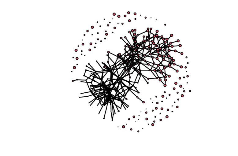
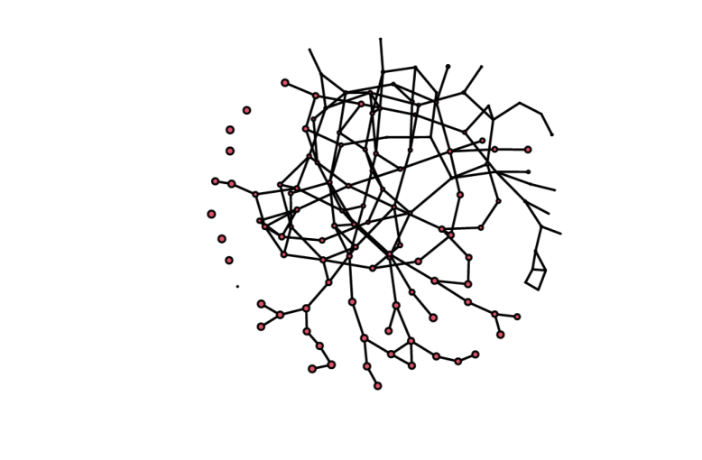
Table 4 shows a comparison of mean network summary statistics, normalized for network size, for the simulated networks. For definitions see the R package igraph, which was used for calculations (igraph1; igraph2). Broadly, centrality statistics measure the prevalence of highly connected nodes and clustering measures the amount of transitive closure in the network. With our parameter choice, the BA HawkesNet produces much larger networks, this was by design and demonstrates the feasibility of the BA HawkesNet model with larger networks. Currently, the CS HawkesNet, with these model terms, is limited by computational feasibility to networks with around nodes.
| Statistic | BA | CS |
|---|---|---|
| number of nodes | 377.640 | 128.850 |
| degree centrality | 0.005 | 0.040 |
| betweeness centrality | 0.004 | 0.015 |
| closeness centrality | 0.209 | 0.307 |
| eigen centrality | 0.063 | 0.307 |
| global clustering | 0.036 | 0.154 |
| local clustering | 0.043 | 0.148 |
We also note that both global and local clustering is higher for the CS HawkesNet, reflecting increased transitivity. Mean centrality measures are also higher for the CS HawkesNet. We note that for the network produced by the BA model most nodes have very low centrality with more nodes with very high centrality.
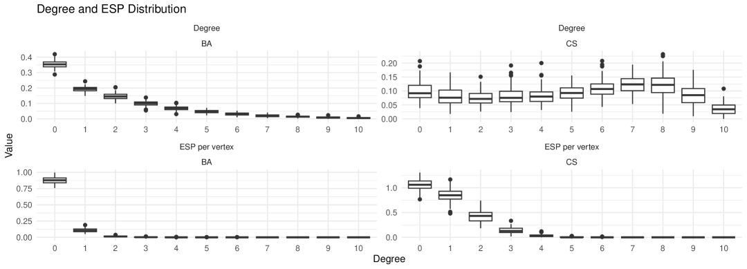
Figure 5 compares the degree and edgewise shared partner (ESP) distribution for each of the true models, normalized for network size. The BA model follows a power law degree distribution, whereas the CS model has a degree distribution with much less right skew. The ESP distribution for the BA HawkesNet networks declines rapidly with the CS model declining much more slowly. This shows that there is significantly more transitivity in the CS model and the BA model has a higher tendency toward more highly connected nodes.
6 Example Data Set
In this section, we fit the CS model to a network of interactions during the first day of the ACM Hypertext 2009 conference (hypertext_conf_1). Edges between conference attendees are present when people are judged to be in close proximity using radio based badges, see sociopatterns2025 for details. There are 100 nodes and 941 edges. Given the intense socialization at such events, we believe modeling updates to the contact network as a HawkesNet to be a reasonable approach.
Most nodes enter early in the time period, with no new nodes added after approximately of the total time period. To model this effectively we fixed the to be after this time. The node arrival time is not a driving factor in edges triggering, for the we let be the time of the last edge involving node rather than the arrival time of node . Table 5 shows the result of fitting the CS model to the data. We note that the triangle parameter estimate is negative, suggesting there is a tendency towards edges not completing triangles. The negative two-star parameter also suggests a tendency against central nodes gaining even more edges, this is mediated by the three-star parameter’s negativity, a phenomenon often observed in ERGM style models (snijders2006). This suggests that most attendees at the conference are perhaps seeking out new connections as they socialize intensely, rather than revisiting connections already close in their social circle.
| Parameter | Estimate | Std. Deviation Estimate |
|---|---|---|
| edges | ||
| triangles | ||
| -star | ||
| -star |
Assessing goodness of fit for marked point processes is difficult, and although various ad-hoc options exist in the literature (clements2011residual; clements2012evaluation; baddeley2005residual; schoenberg2003multidimensional) none are theoretically robust. Rescaled residual are unit Poisson distributed for a correctly specified conditional intensity function via the Random Time Change theorem (daley2003introduction, cf. Proposition 7.4.VI). This result allows for assessment of model fit with respect to the time-dimension, and p-values can be calculated from a Kolmogorov-Smirnov test. Reliable results using this method often require parametric bootstrapping (brown2002time), but more importantly, this approach requires integrating over the mark space, and therefore yields no information with respect to goodness of fit for mark parameters. As an alternative to goodness of fit, predictive information gain metrics are sometimes used for model assessment (davis2024fractional). We therefore leave comprehensive goodness of fit for future work.
7 Discussion
By adapting methods from both the network and point process fields, we have developed a novel framework for modeling time-evolving networks. In this framework, the arrival times of updates to a network are represented as a marked point process, with the marks being updates to the network. Our framework allows highly realistic and expressive modeling; crucially marks and update times can be dependent (non-separable). We demonstrated the ability to apply our simulate and perform MLE-based inference on a wide class of network growth models.
From a network modeling perspective, our approach is the first to provide valid statistical inference for networks with temporally bursty growth. With the increased availability of fine grained temporal network data, our framework unlocks inference for time-evolving networks, without simplifying assumptions. We emphasize that while we have chosen examples with popular network specifications and Hawkesian arrival times, one could posit an arbitrary network growth model with an arbitrary point process specification. The complex interplay between arrival times and network structure sheds light on network model degeneracy. As the kernel function of the Hawkes process temporally decays, it acts as a natural regularizer, preventing degenerate specifications resulting in full graphs.
From a point process perspective, our framework introduces several ideas: most importantly, the notion of a new nonlinear mark path dependent Hawkes process. Nonlinear Hawkes processes have been well studied (bremaud1996stability), but our formulation introduces a novel flavor of nonlinearity that is not captured by a nonlinear “kernel activation function” but rather within the kernel itself through dependence on the history. This structure is crucial for capturing the network evolution as marks. This framework is amenable to a non-separable setting, wherein the temporal evolution and nature of network updates can be intertwined, conditioned on the past history.
This paper introduces a general framework, for which there are many possible extensions that are beyond the scope of this paper. Nodal covariates, often of interest to practitioners, are trivial to include. Currently, we do not allow for repeated edges as might be observed in a typical interaction network; neither do we consider edge dissolution (akin to a birth-death process), which might feasibly be modeled jointly or separately to the edge formation process. A key area of practical focus for future work is computationally facilitating inference for large or online networks. The next step in the theoretical development of our framework is to formally derive stability and stationarity conditions for nonlinear mark path dependent Hawkes processes with network update marks.
8 Acknowledgments
The authors wish to acknowledge the use of New Zealand eScience Infrastructure (NeSI) high performance computing facilities, consulting support and/or training services as part of this research. New Zealand’s national facilities are provided by NeSI and funded jointly by NeSI’s collaborator institutions and through the Ministry of Business, Innovation & Employment’s Research Infrastructure program.
9 Appendix:
9.1 Parametric Examples
Here, we demonstrate stability for various marked Hawkes process kernels, given the heuristic conditions described in Section 3.1.
Example 1.
Let where . In this case, let be a function that counts how many triangles is a part of in the current network. For some positive and moderate time decay parameter , as the network grows, edges increasingly form triangles, and each triangle increases the triggering effect of its component edges. This creates a possibly explosive feedback loop: more edges more triangles, more triangles stronger triggering, stronger triggering more edges. Then
is possible, and in that case the process is explosive and the network density increases without bound. We note here that for network parameters to be identifiable, the network density cannot become infinite.
Example 2.
Let
where is the degree of a node. As , this process explodes (the intensity becomes non-integrable). More generally, the high degree nodes can cause instability quickly. If is sufficiently large (and/or sufficiently small), the process can explode. Such instability can also ensue from non-separable intensities. For instance, let
where is the mean path length and is the mean degree. In this case, the timescale parameter is proportional to network path length (network updates increasing the mean path length have shorter effective timescale), and mark updates increasing the mean degree have faster decay. In this case, stability would imply
which means that the analogous condition for the typical power law kernel is now .
9.2 Nonlinear Hawkes Example: ETAS Model
We justify the notion of mark path dependent processes by illustrating their existence in the context of the highly popular ETAS model ogata1998space. If we specify the conditional intensity
where represents a magnitude completeness cutoff, we have a linear marked Hawkes process. Each point contributes an additive amount to the conditional intensity at time , and the amount of this contribution is a function of . Now consider instead
| (9) |
In the case of a process with conditional intensity as specified in (9), each event’s contribution to the conditional intensity depends not only on its mark, but also on all previous marks. Such a model specification would be sensible if we think that a point with a larger mark might boost or suppress all subsequent events in some way, perhaps in some stress-release sense. The kernel function in (9) is a function of the entire history.
9.3 Additional Induced Models from Network Growth Procedures
Example 3.
Stochastic Block Model HawkesNet
Stochastic block models are a popular framework, with a long history block_models_1; block_models_2; block_models_3 for modeling communities in networks.
We can use a block model inspired method to generate a non separable mark generation density. For a community block model, the model is defined by a vector of group membership probabilities and a matrix where denote the probability of and edge between communities and , with the diagonal being within community edge probabilities.
-
1.
Add a new node set at time
-
2.
Update the community vector with a new entry drawn
-
3.
Connect new nodes with each old node with a time decayed bernoulli variable
Again, the density can be expressed as the product of independent Bernoulli random variables.
An extension of this could allow the group membership parameter to also depend on time and the process.