Fast-dLLM: Training-free Acceleration of Diffusion LLM by Enabling KV Cache and Parallel Decoding

Abstract

Abstract: Diffusion-based large language models (Diffusion LLMs) have shown promise for non-autoregressive text generation. However, the practical inference speed of open-sourced Diffusion LLMs often lags behind autoregressive models due to the lack of Key-Value (KV) Cache and quality degradation when decoding multiple tokens simultaneously. To bridge this gap, we introduce Fast-dLLM, a method that incorporates a novel block-wise approximate KV Cache mechanism tailored for bidirectional diffusion models, enabling cache reuse with negligible performance drop. Additionally, we identify the root cause of generation quality degradation in parallel decoding as the disruption of token dependencies under the conditional independence assumption. To address this, Fast-dLLM also proposes a confidence-aware parallel decoding strategy that selectively decodes tokens exceeding a confidence threshold, mitigating dependency violations and maintaining generation quality. Experimental results on LLaDA and Dream models across multiple LLM benchmarks demonstrate up to 27.6× throughput improvement with minimal accuracy loss, closing the performance gap with autoregressive models and paving the way for practical deployment of Diffusion LLMs.
Links:   Github Code | Project Page

Abstract

Diffusion-based large language models (Diffusion LLMs) have shown promise for non-autoregressive text generation with parallel decoding capabilities. However, the practical inference speed of open-sourced Diffusion LLMs often lags behind autoregressive models due to the lack of Key-Value (KV) Cache and quality degradation when decoding multiple tokens simultaneously. To bridge this gap, we introduce a novel block-wise approximate KV Cache mechanism tailored for bidirectional diffusion models, enabling cache reuse with negligible performance drop. Additionally, we identify the root cause of generation quality degradation in parallel decoding as the disruption of token dependencies under the conditional independence assumption. To address this, we propose a confidence-aware parallel decoding strategy that selectively decodes tokens exceeding a confidence threshold, mitigating dependency violations and maintaining generation quality. Experimental results on LLaDA and Dream models across multiple LLM benchmarks demonstrate up to 27.6$\times$ throughput improvement with minimal accuracy loss, closing the performance gap with autoregressive models and paving the way for practical deployment of Diffusion LLMs.

1 Introduction

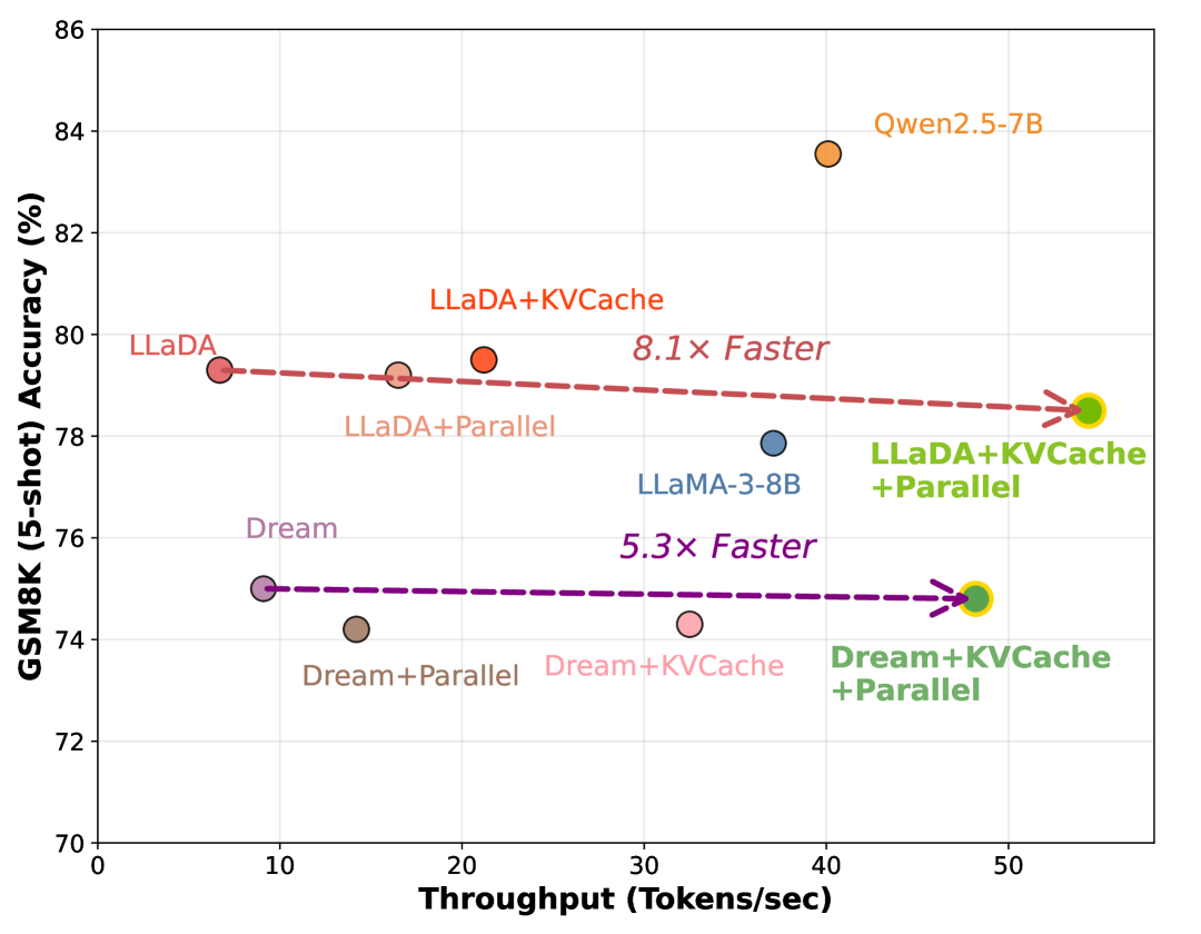
(a) Throughput vs. Accuracy across methods

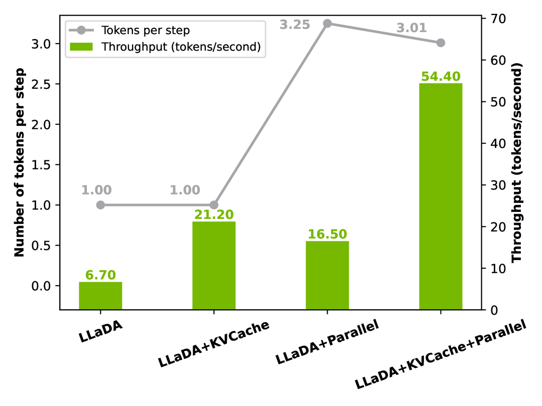
(b) Throughput and tokens per step across methods

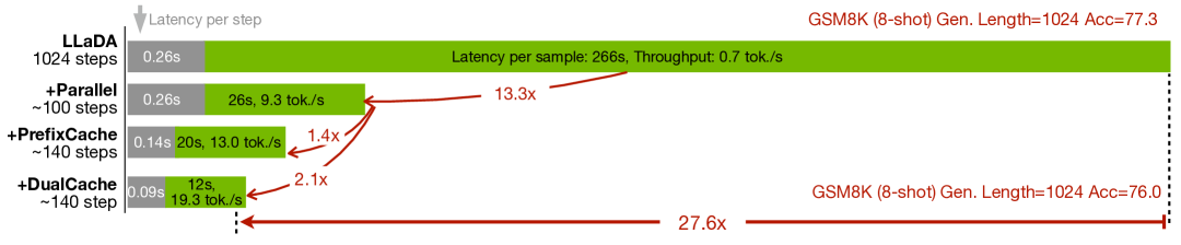
(c) End-to-end speedup over vanilla LLaDA baseline.

Figure 1: Effectiveness of components of Fast-dLLM across different approaches. We use NVIDIA A100 GPU with a single batch size and no inference speedup frameworks.. (a) Inference throughput (tokens/sec) and GSM8K (5-shot) accuracy across various designs and models under a maximum generation length of 256. Caching mechanism and parallel decoding can significantly accelerate inference, while the combination provides up to an 8.1$\times$ increase in throughput with negligible accuracy reduction. (b) We break down the contributions of each method by showing both the number of tokens generated per step (line) and total throughput (bars). (c) With long prefilling (8-shot) and a maximum generation length of 1024, our combined approach achieves up to 27.6$\times$ end-to-end speedup compared to the vanilla LLaDA baseline.

Diffusion-based large language models (Diffusion LLMs) have recently attracted increasing attention due to their potential for parallel token generation and the advantages of bidirectional attention mechanisms. Notably, Mercury mercury2025 runs at over 1,000 tokens per second, and Gemini Diffusion gemini_diffusion2025 by Google DeepMind has demonstrated the ability to generate over 1,400 tokens per second, highlighting the promise of significant inference acceleration.

However, current open-source Diffusion LLMs nie2025largelanguagediffusionmodels ; dream2025 have yet to close such throughput gap in practice, and their actual speed often falls short of autoregressive (AR) models. This is primarily due to two issues. First, diffusion LLMs do not support key-value (KV) caching, a critical component in AR models for speeding up inference. Second, the generation quality tends to degrade when decoding multiple tokens in parallel. For example, recent findings such as those from LLaDA nie2025largelanguagediffusionmodels indicate that Diffusion LLMs perform best when generating tokens one at a time and soon degrades when decoding multiple tokens simultaneously.

To bridge the performance gap with AR models that benefit from KV Cache, we present Fast-dLLM, a fast and practical diffusion-based language modeling framework. First, Fast-dLLM introduces an approximate KV Cache tailored to Diffusion LLMs. While the bidirectional nature of attention in Diffusion LLMs precludes a fully equivalent KV Cache, our approximation closely resembles an ideal cache in practice. To support KV Cache, we adopt a block-wise generation manner. Before generating a block, we compute and store KV Cache of the other blocks to reuse. After generating the block, we recompute the KV Cache of all the blocks. Visualizations confirm the high similarity with adjacent inference steps within the block, and our experiments show that this approximation preserves model performance during inference. We further propose a DualCache version that caches Keys and Values for both prefix and suffix tokens.

In parallel, Fast-dLLM investigates the degradation in output quality when generating multiple tokens simultaneously. Through theoretical analysis and empirical studies, we identify that simultaneous sampling of interdependent tokens under a conditional independence assumption disrupts critical token dependencies. To address this issue and fully exploit the parallelism potential of Diffusion LLMs, we propose a novel confidence-thresholding strategy to select which tokens can be safely decoded simultaneously. Instead of selecting the tokens with top K confidence to decode as in LLaDA, we select tokens with confidence larger than a threshold. Our theoretical justification and experimental results demonstrate that this strategy maintains generation quality while achieving up to 13.3$\times$ inference speed-up.

In summary, our contributions are threefold:

1. Key-Value Cache for Block-Wise Decoding We introduce a block-wise approximate KV Cache mechanism specifically designed for bidirectional attention. Our approach reuses cached activations from previously decoded blocks by exploiting the high similarity of KV activations between adjacent steps. By caching both prefix and suffix blocks, the DualCache strategy enables substantial computational reuse.

2. Confidence-Aware Parallel Decoding We propose a novel confidence-aware parallel decoding method. Unlike prior approaches that select a fixed number of tokens per step, our method dynamically selects tokens whose confidence exceeds a global threshold, enabling safe and effective parallel decoding. This approach significantly accelerates inference by 13.3$\times$ while preserving output quality.

3. State-of-the-Art Acceleration Results We conduct comprehensive experiments on multiple open-source Diffusion LLMs (LLaDA, Dream) and four mainstream benchmarks (GSM8K, MATH, HumanEval, MBPP). Results demonstrate that our Fast-dLLM consistently deliver order-of-magnitude speedups with minimal or no degradation in accuracy, confirming the generality and practical value of our approach for real-world deployment. Fast-dLLM achieves hgiher acceleration (up to 27.6$\times$) when generation length is longer ($1024$).

2 Preliminary

2.1 Masked Diffusion Model

Diffusion models for discrete data were first explored in sohl2015deep ; hoogeboom2021argmax . Subsequently, D3PM austin2021structured proposed a more general framework, defining the forward noising process via a discrete state Markov chain with specific transition matrices $\boldsymbol{Q}_{t}$, and parameterized $p_{\theta}(\boldsymbol{x}_{0}|\boldsymbol{x}_{t})$ for learning the reverse process by maximizing the Evidence Lower Bound (ELBO). CTMC campbell2022continuous further extended D3PM to continuous time, formalizing it within a continuous-time Markov Chain (CTMC) framework. In a different approach, SEDD lou2023discrete parameterizes the likelihood ratio $\frac{p_{t}(\boldsymbol{y})}{p_{t}(\boldsymbol{x})}$ for learning the reverse process, and employs Denoising Score Entropy to train this ratio.

Among the various noise processes in discrete diffusion, Masked Diffusion Models (MDMs), also termed absorbing state discrete diffusion models, have gained considerable attention. MDMs employ a forward noising process where tokens are progressively replaced by a special $[\text{MASK}]$ token. This process is defined by the transition probability:

$$q_{t|0}\left(\boldsymbol{x}_{t}|\boldsymbol{x}_{0}\right)=\prod_{i=1}^{n}q_{t|0}\left(\boldsymbol{x}_{t}^{i}|\boldsymbol{x}_{0}^{i}\right)=\prod_{i=1}^{n}\text{Cat}\left(\boldsymbol{x}_{t}^{i};(1-t)\delta_{\boldsymbol{x}_{0}^{i}}+t\delta_{[\text{MASK}]}\right).$$ (1)

Here, $t\in[0,1]$ denotes the diffusion time (or masking level), controlling the interpolation between the original data $\boldsymbol{x}_{0}$ (at $t=0$) and a fully masked sequence (at $t=1$).

More recently, work by MDLM shi2024simplified ; sahoo2024simple ; zheng2024masked and RADD ou2024your has shown that for MDMs, different parameterizations are equivalent. Furthermore, they demonstrated that the training objective for MDMs can be simplified or directly derived from the data likelihood. This leads to the following objective function, an Evidence Lower Bound (ELBO) on $\log p_{\boldsymbol{\theta}}(\boldsymbol{x})$:

$$-\log p_{\boldsymbol{\theta}}\left(x\right)\leq\int_{0}^{1}\frac{1}{t}\mathbb{E}_{q_{t|0}\left(\boldsymbol{x}_{t}|\boldsymbol{x}_{0}\right)}\left[\sum_{i:\boldsymbol{x}_{0}^{i}=[\text{MASK}]}-\log p_{\boldsymbol{\theta}}(\boldsymbol{x}_{0}^{i}|\boldsymbol{x}_{t})\right]\mathrm{d}t\coloneqq\mathcal{L}_{\text{MDM}}.$$ (2)

2.2 Generation Process of MDMs

The analytical reverse of the forward process defined in Equation 1 is computationally inefficient for generation, as it typically involves modifying only one token per step campbell2022continuous ; lou2023discrete . A common strategy to accelerate this is to employ a $\tau$-leaping gillespie2001approximate approximation for the reverse process. In the context of MDMs, this allows for an iterative generation process where multiple masked tokens can be approximately recovered in a single step from a noise level $t$ to an earlier level $s<t$.

$$q_{s|t}=\prod_{i=0}^{n-1}q_{s|t}(\boldsymbol{x}_{s}^{i}|\boldsymbol{x}_{t}),\text{ where }q_{s|t}(\boldsymbol{x}_{s}^{i}|\boldsymbol{x}_{t})=\begin{cases}1,&\boldsymbol{x}_{t}^{i}\neq[\text{MASK}],\boldsymbol{x}_{s}^{i}=\boldsymbol{x}_{t}^{i}\\ \frac{s}{t},&\boldsymbol{x}_{t}^{i}=[\text{MASK}],\boldsymbol{x}_{s}^{i}=[\text{MASK}]\\ \frac{t-s}{t}q_{0|t}(\boldsymbol{x}_{s}^{i}|\boldsymbol{x}_{t}),&\boldsymbol{x}_{t}^{i}=[\text{MASK}],\boldsymbol{x}_{s}^{i}\neq[\text{MASK}].\end{cases}$$ (3)

Here, $q_{0|t}(\boldsymbol{x}_{s}^{i}|\boldsymbol{x}_{t})$ (when $\boldsymbol{x}_{t}^{i}=[\text{MASK}]$) represents a distribution over the vocabulary for predicting a non-$[\text{MASK}]$ token, provided by the model. In scenarios involving conditional data, such as generating a response $\boldsymbol{x}_{0}$ to a prompt $p$, the MDM’s reverse process, as defined in Equation 3, requires adaptation. Specifically, the model’s predictive distribution $q_{0|t}(\boldsymbol{x}_{s}^{i}|\boldsymbol{x}_{t})$ for unmasking a token $\boldsymbol{x}_{s}^{i}$ is now also conditioned on the prompt $p$, as $q_{0|t}(\boldsymbol{x}_{s}^{i}|\boldsymbol{x}_{t},p)$.

Curse of Parallel Decoding

Directly reversing the forward process from Equation 1 for generation is slow, typically altering just one token per step campbell2022continuous ; lou2023discrete . A common strategy to accelerate this is to employ a $\tau$-leaping gillespie2001approximate approximation for the reverse process. For MDMs, this means multiple masked tokens will be generated in parallel in a single step. However, a significant challenge arises in multiple token prediction due to the conditional independence assumption. Consider an example from song2025ideas : The list of poker hands that consist of two English words are: $\_\ \_$. The subsequent two words could be, for instance, “high card,” “two pair,” “full house,” or “straight flush.” Notably, a correlation exists between these two words. However, the multi-token prediction procedure in MDMs first generates a probability distribution for each token and then samples from these distributions independently. This independent sampling can lead to undesirable combinations, such as “high house.”

To formalize this, consider unmasking two token positions, $i$ and $j$. MDMs sample these from $p(\boldsymbol{x}_{s}^{i}|\boldsymbol{x}_{t})\cdot p(\boldsymbol{x}_{s}^{j}|\boldsymbol{x}_{t})$ due to the conditional independence assumption. However, the true joint probability requires accounting for the dependency: $p(\boldsymbol{x}_{s}^{i},\boldsymbol{x}_{s}^{j}|\boldsymbol{x}_{t})=p(\boldsymbol{x}_{s}^{i}|\boldsymbol{x}_{t})\cdot p(\boldsymbol{x}_{s}^{j}|\boldsymbol{x}_{t},\boldsymbol{x}_{s}^{i})$ (or symmetrically, by conditioning $i$ on $j$). This discrepancy between the assumed independent generation and the true dependent data distribution can degrade the quality and coherence of the generated sequences. The issue is more problematic when a large number of tokens are unmasked simultaneously in a single step.

3 Methodology

3.1 Pipeline Overview

Our approach, Fast-dLLM, builds on the Masked Diffusion Model (MDM) architecture to enable efficient and high-quality sequence generation. To accelerate inference, the overall pipeline incorporates two key strategies: efficient attention computation through Key-Value (KV) Cache and a parallel decoding scheme guided by prediction confidence.

Specifically, we adopt Key-Value Cache for Block-Wise Decoding, which allows reusing attention activations across steps and significantly reduces redundant computation. Within each block, we further propose Confidence-Aware Parallel Decoding, enabling selective updates of tokens based on confidence scores to improve efficiency while maintaining output quality.

By combining these strategies, Fast-dLLM significantly speeds up inference for MDMs with minimal impact on generation performance. The overall procedure is summarized in Algorithm 1.

3.2 Key-Value Cache for Block-Wise Decoding

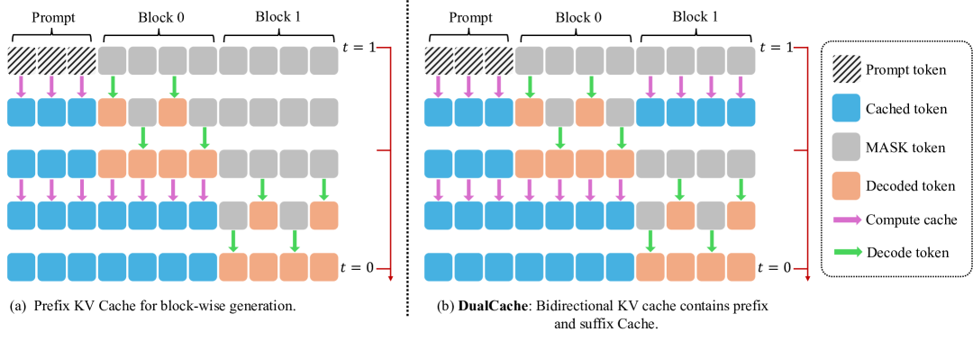
Figure 2: Illustration of our Key-Value Cache for Block-Wise Decoding. (a) During prefix-only caching, the KV cache is computed once for the prompt and reused across multiple decoding steps within each block. The cache is updated after completing a block to maintain consistency, with negligible overhead. (b) DualCache extends this approach by caching both prefix and masked suffix tokens, further accelerating decoding. The high similarity of KV activations across steps allows effective reuse with minimal approximation error.

As shown in Figure 2, we adopt a block-wise decoding strategy to support the use of a Key-Value (KV) Cache. Initially, we compute and store the KV Cache for the prompt, which is reused throughout Block $0$. Within each block, the same cache is reused for multiple decoding steps. After completing the decoding of a block, we update the cache for all tokens (not just the newly generated ones). This cache update can be performed jointly with the decoding step, so compared to not using caching, there is no additional computational overhead. This approach results in an approximate decoding process, due to the use of full attention in masked diffusion models nie2025largelanguagediffusionmodels ; dream2025 .

The effectiveness of our approximate KV Cache approach stems from the observation that KV activations exhibit high similarity across adjacent inference steps, as illustrated in Figure 3. The red boxed region in Figure 3(a) highlights the similarity scores within a block, which are consistently close to 1. This indicates that the differences in prefix keys and values during block decoding are negligible, allowing us to safely reuse the cache without significant loss in accuracy.

Furthermore, we implement a bidirectional version of our KV caching mechanism, named DualCache, that caches not only the prefix tokens but also the suffix tokens, which consist entirely of masked tokens under our block-wise decoding scheme. As shown in Table 4.3, DualCache results in further acceleration. The red boxed region in Figure 3(b) further demonstrates that the differences in suffix keys and values during block decoding are negligible.

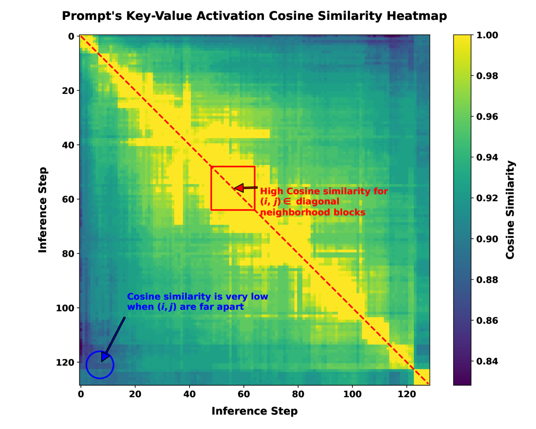
(a) Prompt block

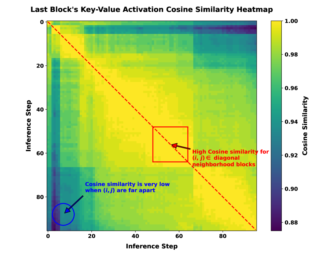
(b) Last block

Figure 3: Heatmaps of Key-Value Activation Cosine Similarity Across Inference Steps in LLaDA-Instruct. (a) Cosine similarity heatmap for the prompt block, averaged over all prompt tokens. (b) Cosine similarity heatmap for the last block, averaged over all tokens in the last block (used to represent suffix tokens, as the last block always belongs to the suffix before its own decoding). In both (a) and (b), high similarity is observed near the diagonal ($i\approx j$), indicating that Key-Value activations at adjacent inference steps within a block are highly similar. The red boxed regions highlight this effect, supporting the use of an approximate block-wise KV Cache: cached activations from previous steps can be safely reused during block decoding with minimal loss in accuracy. The DualCache strategy, which additionally caches suffix tokens, further demonstrates negligible differences in activations during block decoding, enabling greater acceleration with competitive accuracy

3.3 Confidence-Aware Parallel Decoding

While approaches like employing auxiliary models to explicitly capture these dependencies exist liu2024discrete ; xu2024energy , they typically increase the complexity of the overall pipeline. In contrast to these approaches, we propose a simple yet effective confidence-aware decoding algorithm designed to mitigate this conditional independence issue.

Concretely, at each iteration, rather than aggressively unmasking all masked tokens using their independent marginal probabilities, we compute a confidence score for each token (e.g., the maximum softmax probability). Only those with confidence exceeding a threshold are unmasked in the current step; the rest remain masked and are reconsidered in future steps. If no token’s confidence exceeds the threshold, we always unmask the token with the highest confidence to ensure progress and prevent an infinite loop. This strategy accelerates generation while reducing errors from uncertain or ambiguous predictions.

A critical question, however, is: When is it theoretically justifiable to decode tokens in parallel using independent marginals, despite the true joint distribution potentially containing dependencies? We address this with the following formal result, which characterizes the conditions under which greedy parallel (product of marginal distribution) decoding is equivalent to greedy sequential (true joint distribution) decoding in the high-confidence regime, and quantifies the divergence between the two distributions.

Prior to presenting the theorem, we will define the mathematical notation used in its statement. Let $p_{\boldsymbol{\theta}}(\cdot|E)$ denote the conditional probability mass function (PMF) given by an MDM condition on $E$ (comprising a prompt $p_{0}$ and previously generated tokens). Suppose the model is to predict $n$ tokens for positions $i_{1},\dots,i_{n}$ not in $E$. Let $\boldsymbol{X}=(X_{i_{1}},\dots,X_{i_{n}})$ be the vector of $n$ tokens, where each $X_{i_{j}}$ takes values in vocabulary $\mathcal{V}$. Let $p(\boldsymbol{X}|E)\equiv p_{\boldsymbol{\theta}}(X_{i_{1}},\dots,X_{i_{n}}|E)$ be the joint conditional PMF according to the model. Let $p_{j}(X_{i_{j}}|E)\equiv p_{\boldsymbol{\theta}}(X_{i_{j}}|E)$ be the marginal conditional PMF for position $i_{j}$. Parallel decoding generates tokens using the product of marginals: $q(\boldsymbol{X}|E)=\prod_{j=1}^{n}p_{j}(X_{i_{j}}|E)$. The proof of Theorem 1 and relevant discussions are in Appendix A.

Theorem 1 (Parallel Decoding under High Confidence).

Suppose there exists a specific sequence of tokens $\boldsymbol{x}^{*}=(x_{i_{1}},\dots,x_{i_{n}})$ such that for each $j\in\{1,\dots,n\}$, the model has high confidence in $x_{i_{j}}$: $p_{j}(X_{i_{j}}=x_{i_{j}}|E)>1-\epsilon$ for some small $\epsilon>0$. Then, the following results hold:

1. Equivalence for Greedy Decoding: If $(n+1)\epsilon\leq 1$ (i.e., $\epsilon\leq\frac{1}{n+1}$), then

$$\operatornamewithlimits{argmax}_{\boldsymbol{z}}p(\boldsymbol{z}|E)=\operatornamewithlimits{argmax}_{\boldsymbol{z}}q(\boldsymbol{z}|E)=\boldsymbol{x}^{*}.$$ (4)

This means that greedy parallel decoding (selecting $\operatornamewithlimits{argmax}q$) yields the same result as greedy sequential decoding (selecting $\operatornamewithlimits{argmax}p$).

This bound is tight: if $\epsilon>\frac{1}{n+1}$, there exist distributions $p(\boldsymbol{X}|E)$ satisfying the high-confidence marginal assumption for which $\operatornamewithlimits{argmax}_{\boldsymbol{z}}p(\boldsymbol{z}|E)\neq\operatornamewithlimits{argmax}_{\boldsymbol{z}}q(\boldsymbol{z}|E)$.

2. Distance and Divergence Bounds: Let $p(\cdot|E)$ and $q(\cdot|E)$ be denoted as $p$ and $q$ for brevity.

$L_{p}$ Distance ($p\geq 1$): For $n>1$, $D_{p}\left(p,q\right)<((n-1)^{p}+2n)^{1/p}\epsilon$. Specifically, for Total Variation Distance ($D_{TV}(p,q)=\frac{1}{2}D_{1}\left(p,q\right)$): $D_{TV}(p,q)<\frac{3n-1}{2}\epsilon$.

Forward KL Divergence: For $n>1$, $D_{\mathrm{KL}}\left(p\|q\right)<(n-1)(H_{b}(\epsilon)+\epsilon\ln(|\mathcal{V}|-1))$, where $H_{b}(\epsilon)=-\epsilon\ln\epsilon-(1-\epsilon)\ln(1-\epsilon)$ is the binary entropy function, and $|\mathcal{V}|$ is the size of the vocabulary.

Algorithm 1 Block-wise Confidence-aware Parallel Decoding with (Dual) KV Cache

1:$p_{\boldsymbol{\theta}}$, prompt $p_{0}$, answer length $L$, blocks $K$, block size $B$, steps per block $T$, threshold $\tau$, use_DualCache

2:$x\leftarrow[p_{0};\texttt{[MASK]},...,\texttt{[MASK]}]$

3:Initialize KV Cache (single or dual) for $x$ (fuse with decoding). // KV Cache Init

4:for $k=1$ to $K$ do

5:  $s\leftarrow|p_{0}|+(k-1)B$,  $e\leftarrow|p_{0}|+kB$

6:  for $t=1$ to $T$ do

7:   Use cache, run $p_{\boldsymbol{\theta}}$ on $x^{[s,e)}$ if use_DualCache else $x^{[s,:)}$ // Cache Reuse

8:   For masked $x^{i}$, compute confidence $c^{i}=\max_{x}p_{\boldsymbol{\theta}}(x^{i}|\cdot)$ // Confidence scoring

9:   Unmask all $i$ in $[s,e)$ with $c^{i}\geq\tau$, always unmask max $c^{i}$ // Parallel decoding

10:   if all $x^{[s,e)}$ unmasked then

11:     break

12:   end if

13:  end for

14:  Update KV cache: if use_DualCache: prefix & suffix; else: prefix. // Cache Update

15:end for

16:return $x$

4 Experiments

Table 1: Comprehensive benchmark results on the LLaDA-Instruct suite. Each cell presents the accuracy and the decoding throughput in tokens per second with relative speedup to the LLaDA baseline (bottom row, blue: tokens per second/orange: relative speedup). The highest throughput and speedup for each configuration are highlighted.

Benchmark	Gen Length	LLaDA	+Cache	+Parallel	+Cache+Parallel (Fast-dLLM)
GSM8K (5-shot)	256	79.3	79.5	79.2	78.5
		6.7 (1$\times$)	21.2 (3.2$\times$)	16.5 (2.5$\times$)	54.4 (8.1$\times$)
	512	77.5	77.0	77.6	77.2
		3.2 (1$\times$)	10.4 (3.3$\times$)	18.6 (5.8$\times$)	35.3 (11.0$\times$)
MATH (4-shot)	256	33.5	33.3	33.4	33.2
		9.1 (1$\times$)	23.7 (2.6$\times$)	24.8 (2.7$\times$)	51.7 (5.7$\times$)
	512	37.2	36.2	36.8	36.0
		8.0 (1$\times$)	19.7 (2.5$\times$)	23.8 (3.0$\times$)	47.1 (5.9$\times$)
HumanEval (0-shot)	256	41.5	42.7	43.9	43.3
		30.5 (1$\times$)	40.7 (1.3$\times$)	101.5 (3.3$\times$)	114.1 (3.7$\times$)
	512	43.9	45.7	43.3	44.5
		18.4 (1$\times$)	29.3 (1.6$\times$)	57.1 (3.1$\times$)	73.7 (4.0$\times$)
MBPP (3-shot)	256	29.4	29.6	28.4	28.2
		6.0 (1$\times$)	17.0 (2.8$\times$)	24.8 (4.1$\times$)	44.8 (7.5$\times$)
	512	14.8	13.4	15.0	13.8
		4.3 (1$\times$)	10.1 (2.3$\times$)	22.3 (5.1$\times$)	39.5 (9.2$\times$)

Table 2: Comprehensive benchmark results on Dream-Base variants over four tasks with different generation lengths (256 and 512). Each cell shows accuracy (top row) and decoding throughput in tokens per second with relative speedup to Dream-Base baseline (bottom row, blue: tokens per second/orange: relative speedup). Numbers in yellow indicate the highest throughput and speedup per configuration.

Benchmark	Gen Length	Dream	+Cache	+Parallel	+Cache+Parallel (Fast-dLLM)
GSM8K (5-shot)	256	75.0	74.3	74.2	74.8
		9.1 (1$\times$)	32.5 (3.6$\times$)	14.2 (1.6$\times$)	48.2 (5.3$\times$)
	512	76.0	74.3	73.4	74.0
		7.7 (1$\times$)	25.6 (3.3$\times$)	14.6 (1.9$\times$)	42.9 (5.6$\times$)
MATH (4-shot)	256	38.4	36.8	37.9	37.6
		11.4 (1$\times$)	34.3 (3.0$\times$)	27.3 (2.4$\times$)	66.8 (5.9$\times$)
	512	39.8	38.0	39.5	39.3
		9.6 (1$\times$)	26.8 (2.8$\times$)	31.6 (3.2$\times$)	63.3 (6.5$\times$)
HumanEval (0-shot)	256	49.4	53.7	49.4	54.3
		23.3 (1$\times$)	35.2 (1.5$\times$)	45.6 (2.0$\times$)	62.0 (2.8$\times$)
	512	54.3	54.9	51.8	54.3
		16.3 (1$\times$)	27.8 (1.7$\times$)	29.8 (1.8$\times$)	52.8 (3.2$\times$)
MBPP (3-shot)	256	56.6	53.2	53.8	56.4
		11.2 (1$\times$)	34.5 (3.1$\times$)	31.8 (2.8$\times$)	76.0 (6.8$\times$)
	512	55.6	53.8	55.4	55.2
		9.4 (1$\times$)	26.7 (2.8$\times$)	37.6 (4.0$\times$)	73.6 (7.8$\times$)

4.1 Experimental Setup

All experiments are conducted on an NVIDIA A100 80GB GPU. The proposed approach, Fast-dLLM, comprises two components: a Key-Value Cache mechanism and a Confidence-Aware Parallel Decoding strategy. The KV Cache component introduces a hyperparameter, the cache block size, varied between 4 and 32. The parallel decoding strategy uses a confidence threshold hyperparameter, explored in the range of 0.5 to 1.0. Unless otherwise specified, we use PrefixCache with block size of 32 and the threshold to 0.9.

We evaluate Fast-dLLM on two recent diffusion-based language models: LLaDA nie2025largelanguagediffusionmodels and Dream dream2025 . Benchmarks include four widely-used datasets—GSM8K, MATH, HumanEval, and MBPP—to assess performance across diverse reasoning and code generation tasks. We also test under varying generation lengths to evaluate scalability and robustness.

Inference throughput is measured as the average number of output tokens generated per second, calculated over the full sequence until the end-of-sequence (<eos>) token is reached. This metric reflects true end-to-end decoding speed. All evaluations are conducted using the standardized lm-eval library to ensure consistency and reproducibility.

4.2 Main Results: Performance and Speed

We report decoding performance and efficiency gains for Fast-dLLM on both the LLaDA-Instruct and Dream-Base models across the four benchmarks in Tables LABEL:tab:llada_main and 2.

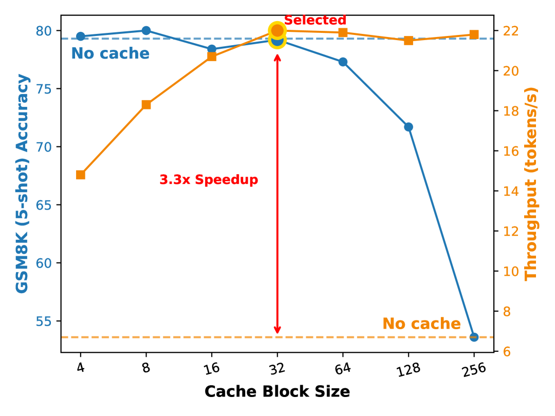
Figure 4: Impact of Cache Block Size on Accuracy and Throughput. The orange line illustrates the effect of varying cache block size on throughput, while the blue line depicts the corresponding impact on accuracy.

Overall, introducing the KV Cache mechanism yields significant speed improvements for all tasks and sequence lengths, typically achieving a $2\times$ to $3.6\times$ speedup compared to the vanilla backbone. When the parallel decoding strategy is applied individually, we see additional acceleration, often pushing speedups to $4\times$–$6\times$ for the evaluated settings, particularly as the generation length increases.

When both techniques are combined, the improvements become even more pronounced. On LLaDA, for example, combined KV Cache and parallel decoding methods boost throughput by up to $11\times$ (GSM8K, length 512) and $9.2\times$ (MBPP, length 512) over the standard baseline. Similarly, on Dream-Base, the largest throughput gains are observed on MBPP ($7.8\times$ at length 512) and GSM8K ($5.6\times$ at length 512). These results indicate that not only are our methods effective individually, but they are also highly complementary, resulting in the combined acceleration.

Figure 5: (a) The red line shows the GSM8K (5-shot) accuracy across different confidence thresholds. Numbers along the red line indicate the average number of tokens decoded at each step. The three dashed lines represent the accuracy of the baseline method when selecting the top 2, 4, or 8 tokens per step. (b) The number of inference steps required under varying confidence thresholds. (c) A comparison between our method and the baseline on GSM8K (5-shot) accuracy, plotted against the average number of tokens per step. Our method consistently outperforms the baseline.

Importantly, these efficiency gains are achieved with negligible impact on accuracy. Across all benchmarks and settings, the accuracy of our accelerated methods remains within 1–2 points of the backbone, and in several cases, accuracy is even slightly improved. This demonstrates that the speedup comes at almost no cost to task performance, ensuring reliability for practical deployment. We also observe that longer sequences, which are common in few-shot and code generation scenarios, benefit proportionally more from our caching and parallelization techniques due to greater opportunities for cache reuse and batch computation.

Furthermore, the improvements generalize across model architectures (LLaDA and Dream) and task types (math reasoning, program synthesis, etc.), confirming that Fast-dLLM is a practical and broadly applicable framework for accelerating masked diffusion-based language models.

4.3 Ablations and Analysis

Table 3: Performance and Speedup Comparison on LLaDA Between 5-Shot and 8-Shot Settings at Generation Length 1024. This table compares the accuracy and throughput speedups of different decoding strategies under 5-shot and 8-shot configurations using a generation length of 1024. The results demonstrate how increased prefill length enhances the effectiveness of caching strategies, particularly for DualCache.

Setting.	LLaDA	Parallel Decoding
		No Cache	PrefixCache	DualCache
5-shot	77.0	77.4	75.2	74.7
	1.1 (1×)	11.7 (10.6×)	14.4 (13.1×)	21.6 (19.6×)
8-shot	77.3	78.0	75.7	76.0
	0.7 (1×)	9.3 (13.3×)	13.0 (18.6×)	19.3 (27.6×)

Table 4: Impact of Generation Length on Accuracy and Speedup Under 8-Shot for LLaDA. This table illustrates the effect of varying generation lengths (256, 512, and 1024) on decoding performance and efficiency for different caching strategies under the 8-shot setting. Longer generation lengths lead to higher throughput gains, especially for DualCache, validating the scalability of our approach.

Len.	LLaDA	Parallel Decoding
		No Cache	PrefixCache	DualCache
256	77.6	77.9	77.3	76.9
	4.9 (1×)	16.4 (3.3×)	49.2 (10.0×)	46.3 (9.4×)
512	78.9	78.9	74.8	75.4
	2.3 (1×)	14.0 (6.1×)	32.0 (13.9×)	36.4 (15.8×)
1024	77.3	78.0	75.7	76.0
	0.7 (1×)	9.3 (13.3×)	13.0 (18.6×)	19.3 (27.6×)

We conduct extensive ablation studies to understand how different components of Fast-dLLM contribute to performance, focusing on factors such as prefill length, generation length, cache mechanism variants, cache block size, and confidence thresholds.

Influence of Prefill and Generation Length on Acceleration

Table 4.3 and Table 4.3 indicate that both prefill length (n-shot) and generation length markedly impact overall speedup. Specifically, as the prefill length increases from 5-shot to 8-shot, the speedup obtained by both versions of KV Cache rises significantly (e.g., speedup for DualCache increases from 19.6$\times$ in 5-shot to 27.6$\times$ in 8-shot for generation length 1024). Similarly, extending the generation length amplifies the potential for cache reuse, leading to higher speedup. Notably, for 8-shot, speedup with DualCache grows from 9.4$\times$ (gen len 256) up to 27.6$\times$ (gen len 1024). This aligns with the theoretical expectation that amortizing computation over longer sequences yields more pronounced efficiency gains.

Comparison of prefix KV Cache vs. DualCache

We further compare our prefix KV Cache and DualCache versions in multiple settings. As shown in Table 4.3, DualCache generally achieves higher speedup than the prefix KV Cache, especially for longer generation lengths. For gen len 512 and 1024, DualCache demonstrates up to 27.6$\times$ speedup, outperforming the prefix KV Cache’s 18.6$\times$ in the same scenario. Importantly, DualCache maintains competitive accuracy, with only minor trade-offs relative to the cache-only variant. This highlights DualCache’s effectiveness in exploiting parallelism and cache locality for both efficiency and accuracy.

Effect of Cache Block Size

Figure 4 analyzes the influence of the cache block size hyperparameter. We observe that smaller block sizes tend to maximize accuracy but incur overhead due to frequent cache updates. In contrast, larger block sizes may diminish accuracy owing to increased context mismatch. Block size of 32 achieves the best trade-off, substantially improving throughput while largely preserving accuracy. This hyperparameter thus offers a practical knob for balancing latency and precision in real deployments.

Dynamic Threshold vs. Fixed Token-per-Step Strategies

Finally, we evaluate our Confidence-Aware Parallel Decoding method against fixed token-per-step baselines on GSM8K (Figure 5). Our adaptive strategy consistently outperforms fixed baselines across key metrics: it delivers higher accuracy at comparable or reduced number of function evaluations (NFE) and generates more tokens per step on average while closely tracking accuracy. In the rightmost panel, the dynamic method approaches or exceeds the accuracy of the 1-token (non-parallel) baseline, but with much greater throughput. The result demonstrates the effectiveness of Confidence-Aware Parallel Decoding, offering practical advantages.

5 Related Work

5.1 Diffusion LLM

Diffusion models have emerged as a transformative paradigm in generative modeling, initially achieving remarkable success in continuous domains such as image rombach2022highresolutionimagesynthesislatent ; nichol2022glidephotorealisticimagegeneration ; ramesh2021zeroshottexttoimagegeneration ; saharia2022photorealistictexttoimagediffusionmodels and audio synthesis yang2023diffsounddiscretediffusionmodel ; huang2023makeanaudiotexttoaudiogenerationpromptenhanced before expanding into natural language processing. Recent advancements in discrete diffusion models austin2021structured ; nie2025scalingmaskeddiffusionmodels ; nie2025largelanguagediffusionmodels ; hoogeboom2021argmax ; campbell2022continuous ; he2022diffusionbert ; meng2022concrete ; reid2022diffuser ; sun2022score ; kitouni2023disk ; zheng2023judging ; chen2023fast ; ye2023diffusion ; sahoo2024simple ; shi2024simplified ; zheng2024masked ; gat2024discrete have reshaped the landscape of text generation, offering a viable alternative to autoregressive (AR) paradigms in large language models (LLMs). These models address the inherent challenges of discrete data by redefining noise injection and denoising processes through innovative mathematical formulations.

Theoretical Foundations of Discrete Diffusion Diffusion models for discrete data were first explored in sohl2015deep ; hoogeboom2021argmax . Subsequently, D3PM austin2021structured provided a more general framework. This framework models the forward noising process as a discrete state Markov chain using specific transition matrices. For the reverse process, D3PM learns a parameterized model of the conditional probability of the original data given a noised version by maximizing the Evidence Lower Bound (ELBO). CTMC campbell2022continuous further extended D3PM to a continuous-time setting, formalizing it as a continuous-time Markov Chain (CTMC). In a distinct approach, SEDD lou2023discrete learns the reverse process by parameterizing the ratio of marginal likelihoods for different data instances at a given noising timestep. This ratio model is then trained using a Denoising Score Entropy objective. More recently, research on Masked Diffusion Models (MDMs) by MDLM shi2024simplified ; sahoo2024simple ; zheng2024masked and RADD ou2024your has introduced significant clarifications. These studies have demonstrated that different parameterizations of MDMs can be equivalent.

Integration with Pre-trained Language Models A critical breakthrough involves combining discrete diffusion with existing LLM architectures. Diffusion-NAT zhou2023diffusionnatselfpromptingdiscretediffusion unifies the denoising process of discrete diffusion with BART’s lewis2019bartdenoisingsequencetosequencepretraining non-autoregressive decoding, enabling iterative refinement of masked tokens. By aligning BART’s inference with diffusion steps, this approach leverages pre-trained knowledge while maintaining generation speed 20× faster than comparable AR transformers. Similarly, the LLaDA nie2025largelanguagediffusionmodels and DiffuLLaMA gong2024scaling framework scales diffusion to $7$B parameters using masked denoising, while LLaDA and Dream dream2025 demonstrating competitive performance with autoregressive baselines like LLaMA3 grattafiori2024llama3herdmodels through recursive token prediction across diffusion timesteps.

5.2 LLM Acceleration

Key-Value Cache. Key-Value (KV) Cache is a fundamental optimization technique in modern large language model (LLM) inference with Transformer architecture vaswani2017attention . It enables efficient autoregressive text generation by storing and reusing previously computed attention states. However, it is non-trival to apply KV Cache in diffusion langauge models such as LLaDA due to full attention. Block diffusion arriola2025blockdiffusioninterpolatingautoregressive overcomes key limitation of previous diffusion langauge models by generating block-by-block so that key and values of previously decoded blocks can be stored and reused.

Non-Autoregressive Generation Non-autoregressive (NAR) generation marks a fundamental shift from sequential token generation by enabling the simultaneous generation of multiple tokens, significantly accelerating inference xiao2023surveynonautoregressivegenerationneural . Initially introduced for neural machine translation, NAR methods have since been extended to a variety of tasks, including grammatical error correction, text summarization, dialogue systems, and automatic speech recognition. Although NAR generation offers substantial speed advantages over autoregressive approaches, it often sacrifices generation quality. Diffusion LLMs represent a recent paradigm for non-autoregressive text generation; however, prior work nie2025largelanguagediffusionmodels has struggled to realize the expected acceleration due to a notable drop in output quality.

6 Conclusion

In this work, we tackle key limitations in the inference efficiency of Diffusion-based Large Language Models (Diffusion LLMs), which have historically lacked support for KV Cache and exhibited performance degradation during parallel decoding. To bridge the gap with autoregressive models, we propose Fast-dLLM, a diffusion-based framework that introduces an approximate KV Cache mechanism tailored to the bidirectional attention characteristics of Diffusion LLMs, enabled by a block-wise generation scheme. Furthermore, we identify that the main obstacle to effective parallel decoding is the disruption of token dependencies arising from the conditional independence assumption. To address this, Fast-dLLM employs a Confidence-Aware Parallel Decoding strategy that facilitates safe and efficient multi-token generation. Extensive experiments across multiple benchmarks and model baselines (LLaDA and Dream) show that Fast-dLLM achieves up to a 27.6$\times$ speedup with minimal loss in accuracy. These findings offer a practical solution for deploying Diffusion LLMs as competitive alternatives to autoregressive models in real-world applications.

Appendix A Proof

In this section, we will give the comprehensive proof and discussion of Theorem 1.

Proof.

Step 1: Show that $\boldsymbol{x}^{*}$ is the unique maximizer of $q(x)$.

Let $p_{j}^{*}=p_{j}(X_{i_{j}}=x_{i_{j}}|E)$. We are given $p_{j}^{*}>1-\epsilon$. Let $\epsilon^{\prime}_{j}=1-p_{j}^{*}=p_{j}(X_{i_{j}}\neq x_{i_{j}}|E)$. Thus, $\epsilon^{\prime}_{j}<\epsilon$. The product-of-marginals probability mass function (PMF) is

$$q(\boldsymbol{z}|E)=\prod_{j=1}^{n}p_{j}(X_{i_{j}}=z_{j}|E).$$

To maximize $q(\boldsymbol{z}|E)$, we must maximize each term $p_{j}(X_{i_{j}}=z_{j}|E)$ independently. The condition $(n+1)\epsilon\leq 1$ implies $\epsilon\leq 1/(n+1)$. Since $n\geq 1$, it follows that $1/(n+1)\leq 1/2$. So, $\epsilon\leq 1/2$. Therefore, for the chosen $x_{i_{j}}$:

$$p_{j}^{*}=p_{j}(X_{i_{j}}=x_{i_{j}}|E)>1-\epsilon\geq 1-1/2=1/2.$$

This means $x_{i_{j}}$ is the unique maximizer for $p_{j}(\cdot|E)$. So,

$$\operatornamewithlimits{argmax}_{\boldsymbol{z}}q(\boldsymbol{z}|E)=(x_{i_{1}},\dots,x_{i_{n}})=\boldsymbol{x}^{*}.$$

Step 2: Show that $\boldsymbol{x}^{*}$ is the unique maximizer of $p(x)$.

We want to show $p(\boldsymbol{x}^{*}|E)>p(\boldsymbol{z}|E)$ for all $\boldsymbol{z}\neq\boldsymbol{x}^{*}$. Using the Bonferroni inequality:

$$p(\boldsymbol{x}^{*}|E) =p(\cap_{j=1}^{n}\{X_{i_{j}}=x_{i_{j}}\}|E)\geq 1-\sum_{j=1}^{n}p(X_{i_{j}}\neq x_{i_{j}}|E)=1-\sum_{j=1}^{n}\epsilon^{\prime}_{j}.$$

Since $\epsilon^{\prime}_{j}<\epsilon$ for all $j$, we have $\sum_{j=1}^{n}\epsilon^{\prime}_{j}<n\epsilon$. So,

$$p(\boldsymbol{x}^{*}|E)>1-n\epsilon.$$

Now consider any $\boldsymbol{z}=(z_{1},\dots,z_{n})$ such that $\boldsymbol{z}\neq\boldsymbol{x}^{*}$. This means there is at least one index $k$ such that $z_{k}\neq x_{i_{k}}$. The event $\{\boldsymbol{X}=\boldsymbol{z}\}$ is a sub-event of $\{X_{i_{k}}=z_{k}\}$. So,

$$p(\boldsymbol{z}|E)\leq p_{k}(X_{i_{k}}=z_{k}|E).$$

Since $z_{k}\neq x_{i_{k}}$,

$$p_{k}(X_{i_{k}}=z_{k}|E)\leq p_{k}(X_{i_{k}}\neq x_{i_{k}}|E)=\epsilon^{\prime}_{k}<\epsilon.$$

Thus,

$$p(\boldsymbol{z}|E)<\epsilon.$$

For $p(\boldsymbol{x}^{*}|E)>p(\boldsymbol{z}|E)$ to hold, it is sufficient that

$$1-n\epsilon\geq\epsilon,$$

which simplifies to $1\geq(n+1)\epsilon$, or $\epsilon\leq\frac{1}{n+1}$. The theorem assumes $(n+1)\epsilon<1$, which is exactly this condition. The strict inequalities $p(\boldsymbol{x}^{*}|E)\geq 1-\sum\epsilon^{\prime}_{j}>1-n\epsilon$ and $p(\boldsymbol{z}|E)\leq\epsilon^{\prime}_{k}<\epsilon$ ensure that $p(\boldsymbol{x}^{*}|E)>p(\boldsymbol{z}|E)$. Thus,

$$\operatornamewithlimits{argmax}_{\boldsymbol{z}}p(\boldsymbol{z}|E)=\boldsymbol{x}^{*}.$$

Combined with the argmax of $q$, this proves the main statement of Part 1:

$$\operatornamewithlimits{argmax}_{\boldsymbol{z}}p(\boldsymbol{z}|E)=\operatornamewithlimits{argmax}_{\boldsymbol{z}}q(\boldsymbol{z}|E)=\boldsymbol{x}^{*}.$$

Step 3: Tightness of the bound $\frac{1}{n+1}$.

The bound $\epsilon\leq\frac{1}{n+1}$ is tight. This means if $\epsilon>\frac{1}{n+1}$, one can construct a scenario where the marginal conditions $p_{j}(X_{i_{j}}=x_{i_{j}}|E)>1-\epsilon$ hold, but $\operatornamewithlimits{argmax}_{\boldsymbol{z}}p(\boldsymbol{z}|E)\neq\boldsymbol{x}^{*}$ (which is $\operatornamewithlimits{argmax}_{\boldsymbol{z}}q(\boldsymbol{z}|E)$ as long as $\epsilon\leq 1/2$).

Consider a vocabulary $\mathcal{V}=\{0,1\}$ and let $x_{i_{j}}=0$ for all $j$, so $\boldsymbol{x}^{*}=(0,\dots,0)$. For each $j\in\{1,\dots,n\}$, let $\mathbf{e}_{j}$ be the vector with $1$ at position $j$ and $0$ elsewhere. Let $\eta=\frac{1}{n+1}(\epsilon-\frac{1}{n+1})>0$. Set $p(\mathbf{e}_{j}|E)=\frac{1}{n+1}+\frac{1}{n}\eta,\ \forall 1\leq j\leq n$ and $p(\boldsymbol{x}^{*}|E)=\frac{1}{n+1}-\eta$ , then $\boldsymbol{x}^{*}\notin\operatornamewithlimits{argmax}_{\boldsymbol{z}}p(\boldsymbol{z}|E)$. The marginal probabilities are:

$$p_{j}(X_{i_{j}}=1|E) =p(\mathbf{e}_{j}|E)=\frac{1}{n+1}+\frac{1}{n}\eta,\ \forall 1\leq j\leq n.$$

$$p_{j}(X_{i_{j}}=0|E) =1-p_{j}(X_{i_{j}}=1|E)=1-\epsilon_{c}=\frac{n}{n+1}-\frac{1}{n}\eta>1-\epsilon,$$

because

$$\frac{1}{n}\eta=\frac{1}{n(n+1)}(\epsilon-\frac{1}{n+1})<\epsilon-\frac{1}{n+1}$$

So, the marginal condition $p_{j}(X_{i_{j}}=x_{i_{j}}|E)>1-\epsilon$ (with $x_{i_{j}}=0$) holds. As shown, $\operatornamewithlimits{argmax}_{\boldsymbol{z}}p(\boldsymbol{z}|E)$ can be made different from $\boldsymbol{x}^{*}$. Thus, if $\epsilon>\frac{1}{n+1}$, the argmax of $p$ and $q$ may not be the same.

Step 4: Bound the $L_{p}$ distance. Let $A_{j}$ be the event $\{X_{i_{j}}=x_{i_{j}}\}$.

$$D_{p}\left(p,q\right)^{p}=|p(\boldsymbol{x}^{*}|E)-q(\boldsymbol{x}^{*}|E)|^{p}+\sum_{\boldsymbol{z}\neq\boldsymbol{x}^{*}}|p(\boldsymbol{z}|E)-q(\boldsymbol{z}|E)|^{p}.$$

The term $|p(\cap_{j=1}^{n}A_{j}|E)-\prod_{j=1}^{n}p(A_{j}|E)|$ (using $p(A_{j}|E)$ for $p_{j}(X_{i_{j}}=x_{i_{j}}|E)$) can be bounded. Since

$$1-\sum_{j=1}^{n}\epsilon^{\prime}_{j}\leq p(\cap_{j=1}^{n}A_{j}|E)\leq\min_{1\leq j\leq n}p(A_{j}|E)=1-\max_{1\leq j\leq n}\epsilon^{\prime}_{j},$$

$$1-\sum_{j=1}^{n}\epsilon^{\prime}_{j}\leq\prod_{j=1}^{n}(1-\epsilon^{\prime}_{j})=\prod_{j=1}^{n}p(A_{j}|E)\leq 1-\max_{1\leq j\leq n}\epsilon^{\prime}_{j}.$$

Thus,

$$|p(\boldsymbol{x}^{*}|E)-q(\boldsymbol{x}^{*}|E)|<(n-1)\epsilon.$$

For $\boldsymbol{z}\neq\boldsymbol{x}^{*}$: $p(\boldsymbol{z}|E)<\epsilon$ and $q(\boldsymbol{z}|E)<\epsilon$. So,

$$|p(\boldsymbol{z}|E)-q(\boldsymbol{z}|E)|<\epsilon.$$

The sum $\sum_{\boldsymbol{z}\neq\boldsymbol{x}^{*}}|p(\boldsymbol{z}|E)-q(\boldsymbol{z}|E)|$ can be bounded:

$$\sum_{\boldsymbol{z}\neq\boldsymbol{x}^{*}}|p(\boldsymbol{z}|E)-q(\boldsymbol{z}|E)| \leq\sum_{\boldsymbol{z}\neq\boldsymbol{x}^{*}}(p(\boldsymbol{z}|E)+q(\boldsymbol{z}|E))=p(\boldsymbol{X}\neq\boldsymbol{x}^{*}|E)+q(\boldsymbol{X}\neq\boldsymbol{x}^{*}|E).$$

$$p(\boldsymbol{X}\neq\boldsymbol{x}^{*}|E) =1-p(\boldsymbol{x}^{*}|E)<1-(1-\sum_{j=1}^{n}\epsilon^{\prime}_{j})=\sum_{j=1}^{n}\epsilon^{\prime}_{j}<n\epsilon.$$

$$q(\boldsymbol{X}\neq\boldsymbol{x}^{*}|E) =1-q(\boldsymbol{x}^{*}|E)<1-\prod_{j=1}^{n}(1-\epsilon^{\prime}_{j})\leq\sum_{j=1}^{n}\epsilon^{\prime}_{j}<n\epsilon.$$

So,

$$\sum_{\boldsymbol{z}\neq\boldsymbol{x}^{*}}|p(\boldsymbol{z}|E)-q(\boldsymbol{z}|E)|<2n\epsilon.$$

Then,

$$\sum_{\boldsymbol{z}\neq\boldsymbol{x}^{*}}|p(\boldsymbol{z}|E)-q(\boldsymbol{z}|E)|^{p} \leq(\sup_{\boldsymbol{z}\neq\boldsymbol{x}^{*}}|p(\boldsymbol{z}|E)-q(\boldsymbol{z}|E)|)^{p-1}\sum_{\boldsymbol{z}\neq\boldsymbol{x}^{*}}|p(\boldsymbol{z}|E)-q(\boldsymbol{z}|E)|$$

$$<\epsilon^{p-1}(2n\epsilon)=2n\epsilon^{p}.$$

Therefore,

$$D_{p}\left(p,q\right)^{p}<((n-1)\epsilon)^{p}+2n\epsilon^{p}=((n-1)^{p}+2n)\epsilon^{p}.$$

So,

$$D_{p}\left(p,q\right)<((n-1)^{p}+2n)^{1/p}\epsilon.$$

For $p=1$,

$$D_{1}\left(p,q\right)<(n-1+2n)\epsilon=(3n-1)\epsilon.$$

And for Total Variation Distance,

$$D_{TV}(p,q)=\frac{1}{2}D_{1}\left(p,q\right)<\frac{3n-1}{2}\epsilon.$$

Step 4: Bound the forward KL divergence.

$$D_{\mathrm{KL}}\left(p\|q\right)=\sum_{\boldsymbol{z}}p(\boldsymbol{z}|E)\log\frac{p(\boldsymbol{z}|E)}{q(\boldsymbol{z}|E)}=I(X_{i_{1}};\dots;X_{i_{n}}|E).$$

The conditional total correlation can be expanded using the chain rule:

$$I(X_{i_{1}};\dots;X_{i_{n}}|E)=\sum_{k=2}^{n}I(X_{i_{k}};X_{i_{1}},\dots,X_{i_{k-1}}|E).$$

Each term is bounded by the conditional entropy:

$$I(X_{i_{k}};X_{i_{1}},\dots,X_{i_{k-1}}|E)\leq H(X_{i_{k}}|E).$$

The conditional entropy $H(X_{i_{k}}|E)$ is bounded. Since $p_{k}(X_{i_{k}}=x_{i_{k}}|E)>1-\epsilon$, it implies $p_{k}(X_{i_{k}}\neq x_{i_{k}}|E)=\epsilon^{\prime}_{k}<\epsilon$. The entropy is maximized when the remaining probability $\epsilon^{\prime}_{k}$ is spread uniformly, leading to:

$$H(X_{i_{k}}|E)\leq H_{b}(\epsilon^{\prime}_{k})+\epsilon^{\prime}_{k}\ln(|\mathcal{V}|-1)<H_{b}(\epsilon)+\epsilon\ln(|\mathcal{V}|-1).$$

Summing $(n-1)$ such terms (for $k=2,\dots,n$):

$$D_{\mathrm{KL}}\left(p\|q\right)<(n-1)[H_{b}(\epsilon)+\epsilon\ln(|\mathcal{V}|-1)].$$

∎

Remark 1.

Assumption of a Well-Defined Joint $p_{\boldsymbol{\theta}}(X_{i_{1}},\dots,X_{i_{n}}|E)$: The theorem and proof rely on $p_{\boldsymbol{\theta}}(X_{i_{1}},\dots,X_{i_{n}}|E)$ being a well-defined joint probability mass function from which the marginals $p_{\boldsymbol{\theta}}(X_{i_{j}}|E)$ are consistently derived. This implies that the joint PMF is coherent and its definition does not depend on a specific factorization order beyond what is captured by the conditioning on $E$. In practice, while MDM may not strictly satisfy this property, its behavior typically offers a close approximation. The theorem holds for an idealized $p_{\boldsymbol{\theta}}$ that possesses these properties. As MDMs become larger and more powerful, their learned distributions might better approximate such consistency.

Worst-Case Analysis: The conditions and bounds provided in the theorem (e.g., $(n+1)\epsilon\leq 1$) are derived from a worst-case analysis. This means the bounds are guaranteed to hold if the conditions are met, regardless of the specific structure of $p_{\boldsymbol{\theta}}(\boldsymbol{X}|E)$ beyond the high-confidence marginal property. In practice, the actual case might be "better behaved" than the worst-case scenario. For instance, the dependencies between $X_{i_{j}}$ and $X_{i_{k}}$ (given $E$) might be weaker than what the worst-case construction assumes. Consequently, the argmax equivalence (Result 1) might still hold frequently even if $(n+1)\epsilon$ is slightly greater than 1 (but not much larger). The condition identifies a threshold beyond which guarantees break down in the worst case, but practical performance can be more robust. Similarly, the actual $L_{p}$ distances or KL divergence might be smaller than the upper bounds suggest if the true joint $p_{\boldsymbol{\theta}}(\boldsymbol{X}|E)$ is closer to the product of marginals $q(\boldsymbol{X}|E)$ than the worst-case configurations.

Appendix B Case Study

Table 5: Qualitative comparison of responses across methods.

Prompt: A robe takes 2 bolts of blue fiber and half that much white fiber. How many bolts in total does it take?
Original	PrefixCache	DualCache
The robe takes 2 bolts of blue fiber. It also takes half that much white fiber, so it takes 2/2 = 1 bolt of white fiber. In total, the robe takes 2 + 1 = 3 bolts of fiber. So, the value is 3	The robe takes 2 bolts of blue fiber. It also takes half that much white fiber, so it takes 2/2 = 1 bolt of white fiber. In total, the robe takes 2 + 1 = 3 bolts of fiber. So, the value is 3	The robe takes 2 bolts of blue fiber. It also takes half that much white fiber, so it takes 2/2 = 1 bolt of white fiber. In total, it takes 2 bolts + 1 bolt = 3 bolts of fiber. The final result is 3

Table 6: Qualitative comparison of responses with varying block size for DualCache.

Prompt: A robe takes 2 bolts of blue fiber and half that much white fiber. How many bolts in total does it take?
Block Size 8	Block Size 16	Block Size 32
The robe takes 2 bolts of blue fiber. It also takes half that much white fiber, so it takes 2/2 = 1 bolt of white fiber. In total, the robe takes 2 + 1 = 3 bolts of fiber. So, the value is 3	The robe takes 2 bolts of blue fiber. It also takes half that much white fiber, so it takes 2/2 = 1 bolt of white fiber. In total, the robe takes 2 + 1 = 3 bolts of fiber. So, the value is 3	The robe takes 2 bolts of blue fiber. It also takes half that much white fiber, so it takes 2/2 = 1 bolt of white fiber. In total, the robe takes 2 + 1 = 3 bolts of fiber. So, the value is 3

Table 7: Qualitative comparison of responses under different threshold settings.

Prompt: A robe takes 2 bolts of blue fiber and half that much white fiber. How many bolts in total does it take?
Threshold 0.7	Threshold 0.8	Threshold 0.9
The robe takes 2 bolts of blue fiber. It also takes half that much white fiber, so it takes 2/2 = 1 bolt of white fiber. In total, it takes takes 2 + 1 = 3 bolts of fiber. So, the value is 3 (NFE: 9)	The robe takes 2 bolts of blue fiber. It also takes half that much white fiber, so it takes 2/2 = 1 bolt of white fiber. In total, the robe takes 2 + 1 = 3 bolts of fiber. So, the value is 3 (NFE: 12)	The robe takes 2 bolts of blue fiber. It also takes half that much white fiber, so it takes 2/2 = 1 bolt of white fiber. In total, the robe takes 2 + 1 = 3 bolts of fiber. So, the value is 3 (NFE: 20)

B.1 Effect of Caching Strategies on Response Quality

Table 5 qualitatively compares answers from the Original, PrefixCache, and DualCache methods for the arithmetic prompt. All correctly compute the answer (3 bolts), following similar step-by-step reasoning, with only minor differences in phrasing. This shows cache strategies maintain answer accuracy and logical clarity while improving efficiency; semantic fidelity and interpretability are unaffected.

B.2 Effect of Block Size in DualCache

Table 6 examines different block sizes (8, 16, 32) in DualCache. For this arithmetic prompt, all settings yield correct, clearly explained answers with no meaningful output differences. Thus, DualCache is robust to block size for such problems, allowing efficiency improvements without compromising quality.

B.3 Impact of Dynamic Threshold Settings

Table 7 investigates dynamic threshold values (0.7, 0.8, 0.9). The model consistently produces the correct answer and clear explanations, regardless of threshold. While higher thresholds increase computational effort (NFE from 9 to 20), answer quality remains stable, indicating threshold adjustment mainly affects efficiency, not correctness, for straightforward arithmetic questions.

References

- [1] Marianne Arriola, Aaron Gokaslan, Justin T. Chiu, Zhihan Yang, Zhixuan Qi, Jiaqi Han, Subham Sekhar Sahoo, and Volodymyr Kuleshov. Block diffusion: Interpolating between autoregressive and diffusion language models, 2025.
- [2] Jacob Austin, Daniel D Johnson, Jonathan Ho, Daniel Tarlow, and Rianne Van Den Berg. Structured denoising diffusion models in discrete state-spaces. Advances in Neural Information Processing Systems, 34:17981–17993, 2021.
- [3] Andrew Campbell, Joe Benton, Valentin De Bortoli, Thomas Rainforth, George Deligiannidis, and Arnaud Doucet. A continuous time framework for discrete denoising models. Advances in Neural Information Processing Systems, 35:28266–28279, 2022.
- [4] Zixiang Chen, Huizhuo Yuan, Yongqian Li, Yiwen Kou, Junkai Zhang, and Quanquan Gu. Fast sampling via de-randomization for discrete diffusion models. arXiv preprint arXiv:2312.09193, 2023.
- [5] Itai Gat, Tal Remez, Neta Shaul, Felix Kreuk, Ricky TQ Chen, Gabriel Synnaeve, Yossi Adi, and Yaron Lipman. Discrete flow matching. arXiv preprint arXiv:2407.15595, 2024.
- [6] Daniel T Gillespie. Approximate accelerated stochastic simulation of chemically reacting systems. The Journal of chemical physics, 115(4):1716–1733, 2001.
- [7] Shansan Gong, Shivam Agarwal, Yizhe Zhang, Jiacheng Ye, Lin Zheng, Mukai Li, Chenxin An, Peilin Zhao, Wei Bi, Jiawei Han, et al. Scaling diffusion language models via adaptation from autoregressive models. arXiv preprint arXiv:2410.17891, 2024.
- [8] Google DeepMind. Gemini diffusion. https://deepmind.google/models/gemini-diffusion, 2025. Accessed: 2025-05-24.
- [9] Aaron Grattafiori, Abhimanyu Dubey, Abhinav Jauhri, Abhinav Pandey, Abhishek Kadian, Ahmad Al-Dahle, et al. The llama 3 herd of models, 2024.
- [10] Zhengfu He, Tianxiang Sun, Kuanning Wang, Xuanjing Huang, and Xipeng Qiu. Diffusionbert: Improving generative masked language models with diffusion models. arXiv preprint arXiv:2211.15029, 2022.
- [11] Emiel Hoogeboom, Didrik Nielsen, Priyank Jaini, Patrick Forré, and Max Welling. Argmax flows and multinomial diffusion: Learning categorical distributions. Advances in Neural Information Processing Systems, 34:12454–12465, 2021.
- [12] Rongjie Huang, Jiawei Huang, Dongchao Yang, Yi Ren, Luping Liu, Mingze Li, Zhenhui Ye, Jinglin Liu, Xiang Yin, and Zhou Zhao. Make-an-audio: Text-to-audio generation with prompt-enhanced diffusion models, 2023.
- [13] Inception Labs. Introducing mercury: The first commercial diffusion-based language model. https://www.inceptionlabs.ai/introducing-mercury, 2025. Accessed: 2025-05-24.
- [14] Ouail Kitouni, Niklas Nolte, James Hensman, and Bhaskar Mitra. Disk: A diffusion model for structured knowledge. arXiv preprint arXiv:2312.05253, 2023.
- [15] Mike Lewis, Yinhan Liu, Naman Goyal, Marjan Ghazvininejad, Abdelrahman Mohamed, Omer Levy, Ves Stoyanov, and Luke Zettlemoyer. Bart: Denoising sequence-to-sequence pre-training for natural language generation, translation, and comprehension, 2019.
- [16] Anji Liu, Oliver Broadrick, Mathias Niepert, and Guy Van den Broeck. Discrete copula diffusion. arXiv preprint arXiv:2410.01949, 2024.
- [17] Aaron Lou, Chenlin Meng, and Stefano Ermon. Discrete diffusion language modeling by estimating the ratios of the data distribution. arXiv preprint arXiv:2310.16834, 2023.
- [18] Chenlin Meng, Kristy Choi, Jiaming Song, and Stefano Ermon. Concrete score matching: Generalized score matching for discrete data. Advances in Neural Information Processing Systems, 35:34532–34545, 2022.
- [19] Alex Nichol, Prafulla Dhariwal, Aditya Ramesh, Pranav Shyam, Pamela Mishkin, Bob McGrew, Ilya Sutskever, and Mark Chen. Glide: Towards photorealistic image generation and editing with text-guided diffusion models, 2022.
- [20] Shen Nie, Fengqi Zhu, Chao Du, Tianyu Pang, Qian Liu, Guangtao Zeng, Min Lin, and Chongxuan Li. Scaling up masked diffusion models on text, 2025.
- [21] Shen Nie, Fengqi Zhu, Zebin You, Xiaolu Zhang, Jingyang Ou, Jun Hu, Jun Zhou, Yankai Lin, Ji-Rong Wen, and Chongxuan Li. Large language diffusion models, 2025.
- [22] Jingyang Ou, Shen Nie, Kaiwen Xue, Fengqi Zhu, Jiacheng Sun, Zhenguo Li, and Chongxuan Li. Your absorbing discrete diffusion secretly models the conditional distributions of clean data. arXiv preprint arXiv:2406.03736, 2024.
- [23] Aditya Ramesh, Mikhail Pavlov, Gabriel Goh, Scott Gray, Chelsea Voss, Alec Radford, Mark Chen, and Ilya Sutskever. Zero-shot text-to-image generation, 2021.
- [24] Machel Reid, Vincent J. Hellendoorn, and Graham Neubig. Diffuser: Discrete diffusion via edit-based reconstruction, 2022.
- [25] Robin Rombach, Andreas Blattmann, Dominik Lorenz, Patrick Esser, and Björn Ommer. High-resolution image synthesis with latent diffusion models, 2022.
- [26] Chitwan Saharia, William Chan, Saurabh Saxena, Lala Li, Jay Whang, Emily Denton, Seyed Kamyar Seyed Ghasemipour, Burcu Karagol Ayan, S. Sara Mahdavi, Rapha Gontijo Lopes, Tim Salimans, Jonathan Ho, David J Fleet, and Mohammad Norouzi. Photorealistic text-to-image diffusion models with deep language understanding, 2022.
- [27] Subham Sekhar Sahoo, Marianne Arriola, Yair Schiff, Aaron Gokaslan, Edgar Marroquin, Justin T Chiu, Alexander Rush, and Volodymyr Kuleshov. Simple and effective masked diffusion language models. arXiv preprint arXiv:2406.07524, 2024.
- [28] Jiaxin Shi, Kehang Han, Zhe Wang, Arnaud Doucet, and Michalis K Titsias. Simplified and generalized masked diffusion for discrete data. arXiv preprint arXiv:2406.04329, 2024.
- [29] Jascha Sohl-Dickstein, Eric Weiss, Niru Maheswaranathan, and Surya Ganguli. Deep unsupervised learning using nonequilibrium thermodynamics. In International conference on machine learning, pages 2256–2265. PMLR, 2015.
- [30] Jiaming Song and Linqi Zhou. Ideas in inference-time scaling can benefit generative pre-training algorithms. arXiv preprint arXiv:2503.07154, 2025.
- [31] Haoran Sun, Lijun Yu, Bo Dai, Dale Schuurmans, and Hanjun Dai. Score-based continuous-time discrete diffusion models. arXiv preprint arXiv:2211.16750, 2022.
- [32] Ashish Vaswani. Attention is all you need. arXiv preprint arXiv:1706.03762, 2017.
- [33] Yisheng Xiao, Lijun Wu, Junliang Guo, Juntao Li, Min Zhang, Tao Qin, and Tie yan Liu. A survey on non-autoregressive generation for neural machine translation and beyond, 2023.
- [34] Minkai Xu, Tomas Geffner, Karsten Kreis, Weili Nie, Yilun Xu, Jure Leskovec, Stefano Ermon, and Arash Vahdat. Energy-based diffusion language models for text generation. arXiv preprint arXiv:2410.21357, 2024.
- [35] Dongchao Yang, Jianwei Yu, Helin Wang, Wen Wang, Chao Weng, Yuexian Zou, and Dong Yu. Diffsound: Discrete diffusion model for text-to-sound generation, 2023.
- [36] Jiacheng Ye, Zhihui Xie, Lin Zheng, Jiahui Gao, Zirui Wu, Xin Jiang, Zhenguo Li, and Lingpeng Kong. Dream 7b, 2025.
- [37] Jiasheng Ye, Zaixiang Zheng, Yu Bao, Lihua Qian, and Quanquan Gu. Diffusion language models can perform many tasks with scaling and instruction-finetuning. arXiv preprint arXiv:2308.12219, 2023.
- [38] Kaiwen Zheng, Yongxin Chen, Hanzi Mao, Ming-Yu Liu, Jun Zhu, and Qinsheng Zhang. Masked diffusion models are secretly time-agnostic masked models and exploit inaccurate categorical sampling. arXiv preprint arXiv:2409.02908, 2024.
- [39] Lianmin Zheng, Wei-Lin Chiang, Ying Sheng, Siyuan Zhuang, Zhanghao Wu, Yonghao Zhuang, Zi Lin, Zhuohan Li, Dacheng Li, Eric Xing, et al. Judging llm-as-a-judge with mt-bench and chatbot arena. Advances in Neural Information Processing Systems, 36:46595–46623, 2023.
- [40] Kun Zhou, Yifan Li, Wayne Xin Zhao, and Ji-Rong Wen. Diffusion-nat: Self-prompting discrete diffusion for non-autoregressive text generation, 2023.