Cosmological constraints on small-scale primordial non-Gaussianity

Abstract

In contrast to the large-scale primordial power spectrum $\mathcal{P}_{\zeta}(k)$ and primordial non-Gaussianity $f_{\mathrm{NL}}$, which are strictly constrained, the small-scale $\mathcal{P}_{\zeta}(k)$ and $f_{\mathrm{NL}}$ remain less restricted. Considering local-type primordial non-Gaussianity, we study the PBH and SIGW caused by large-amplitude small-scale primordial power spectrum. By analyzing current observational data from PTA, CMB, BAO, and abundance of PBH, and combining them with the SNR analysis of LISA, we rigorously constrain the parameter space of $\mathcal{P}_{\zeta}(k)$ and $f_{\mathrm{NL}}$. Furthermore, we examine the effects of different shapes of the primordial power spectrum on these constraints and comprehensively calculate the Bayes factors for various models. Our results indicate that SIGW generated by a monochromatic primordial power spectrum are more likely to dominate current PTA observations, with the corresponding constraint on the primordial non-Gaussian parameter being $-10.0<f_{\mathrm{NL}}<1.2$.

I Introductions

Our universe originated from primordial perturbations generated during the inflationary era Lyth and Rodriguez (2005); Weinberg (2005); Bassett et al. (2006). These primordial perturbations carry the physical information from the inflationary period, influencing all subsequent evolutionary processes of the universe Baumann (2011); Riotto (2003); Goldwirth and Piran (1992); Malik and Wands (2009); Baumann (2018). Through current cosmological observations on different scales, we can determine the physical properties of primordial perturbations on various scales, providing us with crucial information on new physics during the evolution of the universe Irastorza and Redondo (2018); Cai et al. (2016); Marsh (2016); De Felice and Tsujikawa (2010); Bojowald (2005); Gasperini and Veneziano (2003); Lyth and Riotto (1999); Kim and Carosi (2010).

Over the past few decades, cosmological research has made significant strides Abdalla et al. (2022); Workman et al. (2022); Navas et al. (2024). The cosmological observations, such as CMB, LSS, BBN, and BAO, provide us with a wealth of precise cosmological data, enabling us to accurately determine the physical properties of primordial perturbations Bernardeau et al. (2002); Bartolo et al. (2004); Ade et al. (2014, 2016); Dawson et al. (2016); Aghanim et al. (2020a); Achucarro et al. (2011). Specifically, on large scales ($\gtrsim$1 Mpc), the power spectrum of primordial curvature perturbations is approximately a scale-invariant spectrum, with an amplitude $A_{\zeta}\approx 2\times 10^{-9}$ Aghanim et al. (2020b). Moreover, the current constraint on the tensor-to-scalar ratio $r$ is $r<0.064$ at $95\%$ confidence level Akrami et al. (2020a). Furthermore, as one of the most important properties of primordial perturbations, the non-Gaussianity of the primordial power spectrum on large scales has also been tightly constrained. For instance, the current cosmological observations reveal that the parameter of local-type primordial non-Gaussianity $f_{\mathrm{NL}}=-0.9\pm 5.1$ at $68\%$ confidence level Akrami et al. (2020b). However, unlike large-scale primordial perturbations, there are no strict observational constraints on small-scale ($\lesssim$1 Mpc) primordial perturbations Bringmann et al. (2012). Exploring how to leverage different cosmological observations to constrain the small-scale primordial power spectrum and its associated non-Gaussianity represents one of the foremost challenges in further cosmological research.

Various inflationary models can generate primordial curvature perturbations with significant amplitudes and non-Gaussianity on small scales. Examples include multi-field inflation models Kristiano and Yokoyama (2024); Ballesteros and Taoso (2018); Braglia et al. (2020); Palma et al. (2020); Ballesteros et al. (2020); Atal et al. (2020), Higgs inflation models Kristiano and Yokoyama (2024); Ballesteros and Taoso (2018); Braglia et al. (2020); Palma et al. (2020); Ballesteros et al. (2020); Atal et al. (2020) , and inflation models based on modified gravity theories Pi et al. (2018); Kawai and Kim (2021); Lin et al. (2020); Arya et al. (2024); Bamba and Odintsov (2015); Chen and Gao (2025); Peng et al. (2022). Constraining the primordial curvature perturbations and their associated non-Gaussianity on small scales requires taking into account their impact on small-scale cosmological observables. More precisely, after inflation ends and these large amplitude primordial perturbations re-enter the horizon, they will cause substantial density perturbations that collapse to form PBH Khlopov (2010); Carr et al. (2016); Sasaki et al. (2018); Carr and Kuhnel (2020); De Luca et al. (2021); Musco (2019); Carr et al. (2024); Carr and Kuhnel (2022); Liu et al. (2022); Choudhury et al. (2023); Gouttenoire and Volansky (2024); Belotsky et al. (2014). This process will also inevitably generate SIGW Domènech (2021); Mollerach et al. (2004); Ananda et al. (2007); Baumann et al. (2007). By analyzing the abundance of PBH and the observations of SIGW such as LISA and PTA, we can identify the parameter space for the small-scale primordial power spectrum $\mathcal{P}_{\zeta}\left(k\right)$ and the associated parameter of local-type primordial non-Gaussianity $f_{\mathrm{NL}}$ allowed by current observations.

In this paper, we concentrate on the constraints imposed by current cosmological observations on small-scale local-type primordial non-Gaussianity. Specifically, we consider the following observational constraints:

Using the aforementioned four types of cosmological observations, we can rigorously quantify the constraints on the small-scale primordial power spectrum and primordial non-Gaussianity.

This paper is organized as follows. In Sec. II, we study the energy density spectra of SIGW and analyze the constraints on $\mathcal{P}_{\zeta}(k)$ and $f_{\mathrm{NL}}$ imposed by PTA, LISA, and large-scale cosmological observations. In Sec. III, we calculate the abundance of PBH and examine the impact of PBH abundance on the constraints of $f_{\mathrm{NL}}$. In Sec. IV, we investigate the impact of various forms of the primordial power spectrum on the constraints of $f_{\mathrm{NL}}$. Additionally, we compute the Bayes factors between different models using the current PTA data. Finally, we summarize our results and give some discussions in Sec. V.

II Scalar induced gravitational waves

In June 2023, the PTA collaborations NANOGrav Agazie et al. (2023), EPTA Antoniadis et al. (2023), PPTA Reardon et al. (2023), and the CPTA Xu et al. (2023) reported positive evidence for an isotropic, stochastic background of GW within the nHz frequency range. As mentioned in ref. Afzal et al. (2023), among the numerous potential contributors to the SGWB, SIGW show the highest Bayes factor, which makes them one of the most likely dominant sources. In this case, considering the scenario where SIGW dominate the current nHz frequency band of the SGWB, we perform a Bayesian analysis using the current PTA observational data. This allows us to determine the current PTA constraints on small-scale primordial power spectrum $\mathcal{P}_{\zeta}\left(k\right)$ and the corresponding parameter of local-type primordial non-Gaussianity $f_{\mathrm{NL}}$ Yi et al. (2024); Wang et al. (2024b); Perna et al. (2024); Papanikolaou et al. (2024).

In the case of the local-type primordial non-Gaussianity, the non-Gaussian primordial curvature perturbation can be expressed as a local perturbative expansion around the Gaussian primordial curvature perturbation. In momentum space, the primordial curvature perturbation can be written as Cai et al. (2019); Domènech (2021)

$$\zeta^{\mathrm{ng}}_{\mathbf{k}}=\zeta^{\mathrm{g}}_{\mathbf{k}}+\frac{3}{5}f_{\mathrm{NL}}\int\frac{{\mathop{}\!\mathrm{d}}^{3}n}{(2\pi)^{3/2}}\zeta^{\mathrm{g}}_{\mathbf{k}-\mathbf{n}}\zeta^{\mathrm{g}}_{\mathbf{n}}\ ,$$ (1)

where $\mathbf{n}$ is the three dimensional momentum variable. $\zeta^{\mathrm{g}}_{\mathbf{k}}$ is the Gaussian primordial curvature perturbation.

The second-order SIGW can be expressed as

$$h^{\lambda,(2)}_{\mathbf{k}}(\eta)=\int\frac{\mathop{}\!\mathrm{d}^{3}p}{(2\pi)^{3/2}}\varepsilon^{\lambda,lm}(\mathbf{k})p_{l}p_{m}I^{(2)}\zeta_{\mathbf{k}-\mathbf{p}}\zeta_{\mathbf{p}}\ ,$$ (2)

where $\varepsilon^{\lambda,lm}(\mathbf{k})$$(\lambda=+,\times)$ are polarization tensors. The explicit expressions of the second-order kernel functions $I^{(2)}$ can be found in Ref. Kohri and Terada (2018). By analyzing the two-point correlation function of second-order SIGW, we can determine the corresponding energy density spectrum. The calculation of the two-point correlation function $\langle h^{\lambda,(2)}_{\mathbf{k}}h^{\lambda^{\prime},(2)}_{\mathbf{k}^{\prime}}\rangle$ involves the four-point correlation function associated with primordial curvature perturbations: $\langle\zeta_{\mathbf{k}-\mathbf{p}}\zeta_{\mathbf{p}}\zeta_{\mathbf{k}^{\prime}-\mathbf{p}^{\prime}}\zeta_{\mathbf{p}^{\prime}}\rangle$. Combining the expression of local-type non-Gaussian primordial curvature perturbations provided in Eq. (1), the total energy density spectrum of second-order SIGW can be written as Adshead et al. (2021); Li et al. (2025)

$$\bar{\Omega}^{(2)}_{\mathrm{GW}}(k) =\bar{\Omega}_{\mathrm{GW}}^{G}+\bar{\Omega}_{\mathrm{GW}}^{H}+\bar{\Omega}_{\mathrm{GW}}^{C}+\bar{\Omega}_{\mathrm{GW}}^{Z}$$ (3)

$$+\bar{\Omega}_{\mathrm{GW}}^{R}+\bar{\Omega}_{\mathrm{GW}}^{P}+\bar{\Omega}_{\mathrm{GW}}^{N}\ ,$$

where the energy density spectrum of the second-order SIGW is categorized into seven distinct loop diagram contributions. In Eq. (3), the contributions of Gaussian one-loop diagrams, proportional to $A_{\zeta}^{2}$, are denoted by $\bar{\Omega}_{\mathrm{GW}}^{G}$. The symbols $\bar{\Omega}_{\mathrm{GW}}^{H}$, $\bar{\Omega}_{\mathrm{GW}}^{C}$, and $\bar{\Omega}_{\mathrm{GW}}^{Z}$ denote non-Gaussian contributions of two-loop diagrams proportional to $A_{\zeta}^{3}\left(f_{\mathrm{NL}}\right)^{2}$. The symbols $\bar{\Omega}_{\mathrm{GW}}^{R}$, $\bar{\Omega}_{\mathrm{GW}}^{P}$, and $\bar{\Omega}_{\mathrm{GW}}^{N}$ correspond to non-Gaussian contributions of three-loop diagrams proportional to $A_{\zeta}^{4}\left(f_{\mathrm{NL}}\right)^{4}$. The explicit expressions of these loop diagrams of second-order SIGW in Eq. (3) can be found in Ref. Li et al. (2023).

Furthermore, due to the significant primordial perturbations on small scales, higher-order cosmological perturbations significantly affect the total energy density spectrum of SIGW, thus modifying the parameter space of $\mathcal{P}_{\zeta}(k)$ and $f_{\mathrm{NL}}$ determined by PTA observations. Specifically, the third-order SIGW can be expressed as Zhou et al. (2022); Chang et al. (2023a)

$$h^{\lambda,(3)}_{\mathbf{k}}(\eta) = \sum_{i=1}^{4}h_{i,\mathbf{k}}^{\lambda,(3)}(\eta)=\int\frac{\mathop{}\!\mathrm{d}^{3}p}{(2\pi)^{3/2}}\int\frac{\mathop{}\!\mathrm{d}^{3}q}{(2\pi)^{3/2}}$$ (4)

$$\times \varepsilon^{\lambda,lm}(\mathbf{k})\mathbb{P}^{i}_{lm}I_{i}^{(3)}\zeta_{\mathbf{k}-\mathbf{p}}\zeta_{\mathbf{p}-\mathbf{q}}\zeta_{\mathbf{q}}\ ,$$

where the momentum polynomials $\mathbb{P}^{i}_{lm}$$(i=1,2,3,4)$ are given by

$$\mathbb{P}^{1}_{lm} = q_{m}\left(p_{l}-q_{l}\right)\ ,\ \mathbb{P}^{2}_{lm}=\Lambda_{lm}^{rs}(\mathbf{p})q_{r}q_{s}\ ,$$ (5)

$$\mathbb{P}^{3}_{lm} = \left(\mathcal{T}_{m}^{r}(\mathbf{p})p_{l}+\mathcal{T}_{l}^{r}(\mathbf{p})p_{m}\right)\frac{p^{s}}{p^{2}}q_{r}q_{s}\ ,$$ (6)

$$\mathbb{P}^{4}_{lm} = p_{l}p_{m}\ .$$ (7)

In Eq. (5), $\Lambda_{ij}^{lm}(\mathbf{p})$ represents the transverse and traceless operator, defined as

$$\Lambda_{ij}^{lm}(\mathbf{p})=\mathcal{T}_{i}^{l}(\mathbf{p})\mathcal{T}_{j}^{m}(\mathbf{p})-\frac{1}{2}\mathcal{T}_{ij}(\mathbf{p})\mathcal{T}^{lm}(\mathbf{p})\ ,$$ (8)

where $\mathcal{T}_{ij}(\mathbf{p})=\delta_{ij}-p_{i}p_{j}/p^{2}$. In Eq. (4), the contribution of third-order SIGW consists of four parts, denoted as $h_{i,\mathbf{k}}^{\lambda,(3)}$$(i=1,2,3,4)$. They correspond respectively to the third-order gravitational waves directly induced by first-order scalar perturbations, and to the third-order gravitational waves jointly induced by first-order scalar perturbations and three types of second-order perturbations. The explicit expressions of the third-order kernel functions $I^{(3)}_{i}$$(i=1,2,3,4)$ in Eq. (4) are provided in Ref. Zhou et al. (2022).

When we consider SIGW up to the third order, the two-point correlation function of the gravitational waves can be expressed as

$$\langle h^{\lambda}_{\mathbf{k}}h^{\lambda^{\prime}}_{\mathbf{k}^{\prime}}\rangle = \langle h^{\lambda,(2)}_{\mathbf{k}}h^{\lambda^{\prime},(2)}_{\mathbf{k}^{\prime}}\rangle+\langle h^{\lambda,(3)}_{\mathbf{k}}h^{\lambda^{\prime},(3)}_{\mathbf{k}^{\prime}}\rangle$$ (9)

$$+ 2~\langle h^{\lambda,(3)}_{\mathbf{k}}h^{\lambda^{\prime},(2)}_{\mathbf{k}^{\prime}}\rangle\ .$$

Here, we have ignored the potential large-amplitude primordial gravitational waves on small scales Wu et al. (2024); Fu et al. (2024); Gorji et al. (2023). As previously discussed, in Eq. (9), $\langle h^{\lambda,(2)}_{\mathbf{k}}h^{\lambda^{\prime},(2)}_{\mathbf{k}^{\prime}}\rangle$ represents the two-point correlation function of second-order SIGW, proportional to the four-point correlation function of primordial curvature perturbations: $\langle\zeta_{\mathbf{k}-\mathbf{p}}\zeta_{\mathbf{p}}\zeta_{\mathbf{k}^{\prime}-\mathbf{p}^{\prime}}\zeta_{\mathbf{p}^{\prime}}\rangle$. Similarly, the two-point correlation function of third-order SIGW $\langle h^{\lambda,(3)}_{\mathbf{k}}h^{\lambda^{\prime},(3)}_{\mathbf{k}^{\prime}}\rangle$ is proportional to the six-point correlation function of primordial curvature perturbations: $\langle\zeta_{\mathbf{k}-\mathbf{p}}\zeta_{\mathbf{p}-\mathbf{q}}\zeta_{\mathbf{q}}\zeta_{\mathbf{k}^{\prime}-\mathbf{p}^{\prime}}\zeta_{\mathbf{p}^{\prime}-\mathbf{q}^{\prime}}\zeta_{\mathbf{q}^{\prime}}\rangle$. And the cross-correlation function $\langle h^{\lambda,(3)}_{\mathbf{k}}h^{\lambda^{\prime},(2)}_{\mathbf{k}^{\prime}}\rangle$ is proportional to the five-point correlation function of primordial curvature perturbations: $\langle\zeta_{\mathbf{k}-\mathbf{p}}\zeta_{\mathbf{p}-\mathbf{q}}\zeta_{\mathbf{q}}\zeta_{\mathbf{k}^{\prime}-\mathbf{p}^{\prime}}\zeta_{\mathbf{p}^{\prime}}\rangle$. In addition, the cross two-point correlation function $\langle h^{\lambda,(3)}_{\mathbf{k}}h^{\lambda^{\prime},(2)}_{\mathbf{k}^{\prime}}\rangle$ will only modify the total energy density spectrum of SIGW if primordial non-Gaussianity is present. The lowest-order contribution of this modification is proportional to $A_{\zeta}^{3}f_{\mathrm{NL}}$, corresponding to the two-loop diagrams of SIGW Chang et al. (2024a). In summary, when considering SIGW up to the third order, the corresponding one-loop $(\sim A_{\zeta}^{2})$ and two-loop $(\sim A_{\zeta}^{3})$ contributions can be expressed as

$$\bar{\Omega}^{\mathrm{tot}}_{\mathrm{GW}}(k) = \bar{\Omega}_{\mathrm{GW}}^{G}+\bar{\Omega}_{\mathrm{GW}}^{H}+\bar{\Omega}_{\mathrm{GW}}^{C}+\bar{\Omega}_{\mathrm{GW}}^{Z}$$ (10)

$$+ \bar{\Omega}^{(3)}_{\mathrm{GW}}(k)+2\bar{\Omega}^{(3,2)}_{\mathrm{GW}}(k,\eta)\ .$$

When $f_{\mathrm{NL}}<0$, the contributions of $\bar{\Omega}^{(2,3)}_{\mathrm{GW}}$ can significantly suppress the total energy density spectrum of SIGW. The explicit expressions of third-order corrections $\bar{\Omega}^{(3)}_{\mathrm{GW}}$ and $\bar{\Omega}^{(3,2)}_{\mathrm{GW}}$ can be found in Refs. Chang et al. (2024a, b).

In this study, we focus on the following two types of energy density spectra:

1. The total energy density spectrum of second-order SIGW as described in Eq. (3).

2. The complete one-loop and two-loop contributions involving up to third-order SIGW as presented in Eq. (10).

Furthermore, Eq. (3) and Eq. (10) present the formulas for the energy density spectrum of SIGW during the RD era. Taking into account the thermal history of the universe, we obtain the current energy density spectrum Wang et al. (2019)

$$\bar{\Omega}_{\mathrm{GW,0}}(k)=\Omega_{\mathrm{rad},0}\left(\frac{g_{*,\rho,e}}{g_{*,\rho,0}}\right)\left(\frac{g_{*,s,0}}{g_{*,s,e}}\right)^{4/3}\bar{\Omega}_{\mathrm{GW}}(k)\ ,$$ (11)

where $\Omega_{\mathrm{rad},0}$ ($=4.2\times 10^{-5}h^{-2}$) is the energy density fraction of radiations today. The effect numbers of relativistic species $g_{*,\rho}$ and $g_{*,s}$ can be found in Ref. Saikawa and Shirai (2018). And the dimensionless Hubble constant is $h=0.6736$ Aghanim et al. (2020b).

II.1 PTA observations

Given the specific form of the primordial power spectrum $\mathcal{P}_{\zeta}(k)$, we can calculate the energy density spectrum of SIGW. In this section, we consider the LN primordial power spectrum

$$\mathcal{P}^{\mathrm{LN}}_{\zeta}(k)=\frac{A_{\zeta}}{\sqrt{2\pi\sigma^{2}}}\exp\left(-\frac{1}{2\sigma^{2}}\ln^{2}\left(k/k_{*}\right)\right)\ ,$$ (12)

where $A_{\zeta}$ is the amplitude of primordial power spectrum and $k_{*}=2\pi f_{*}$ is the wavenumber at which the primordial power spectrum has a LN peak. The parameter $\sigma$ indicates the width of the LN primordial power spectrum.

To characterize the parameter space of $\mathcal{P}^{\mathrm{LN}}_{\zeta}(k)$ and $f_{\mathrm{NL}}$ inferred from PTA observations, we construct the likelihood function using KDE representations of the free spectra Mitridate et al. (2023); Lamb et al. (2023); Moore and Vecchio (2021). The likelihood is given by

$$\ln\mathcal{L}(d|\theta)=\sum_{i=1}^{N_{f}}p(\Phi_{i},\theta)\ .$$ (13)

Here $p(\Phi_{i},\theta)$ represents the probability of $\Phi_{i}$ given the parameter $\theta$, and $\Phi_{i}=\Phi(f_{i})$ denotes the time delay

$$\Phi(f)=\sqrt{\frac{H_{0}^{2}\Omega_{\mathrm{GW}}(f)}{8\pi^{2}f^{5}T_{\mathrm{obs}}}}\ ,$$ (14)

where $H_{0}=h\times 100\mathrm{km/s/Mpc}$ is the present-day value of the Hubble constant. We directly use the KDE representation of the first 14 frequency bins of the HD(Helling-Downs)-correlated free spectrum in NANOGrav 15-year dataset Collaboration (2023). Bayesian analysis is performed by bilby Ashton et al. (2019) with its built-in dynesty nested sampler Speagle (2020); Koposov et al. (2024). Furthermore, to investigate the impact of astrophysical sources of the SGWB on current PTA observations, we consider the SGWB generated by SMBHB, with the corresponding energy density spectrum given by Mitridate et al. (2023); Afzal et al. (2023)

$$\Omega^{\mathrm{BH}}_{\mathrm{GW}}(f)=\frac{2\pi^{2}A_{\mathrm{BHB}}^{2}}{3H_{0}^{2}h^{2}}(\frac{f}{\mathrm{year}^{-1}})^{5-\gamma_{\mathrm{BHB}}}\mathrm{year}^{-2}\ .$$ (15)

Here, the prior distribution for $(\log_{10}A_{\mathrm{BHB}},\gamma_{\mathrm{BHB}})$ follows a multivariate normal distribution Afzal et al. (2023), whose mean and covariance matrix are given by

$$\boldsymbol{\mu}_{\mathrm{BHB}}=\begin{pmatrix}-15.6\\ 4.7\end{pmatrix},\boldsymbol{\sigma}_{\mathrm{BHB}}=0.1\begin{pmatrix}2.8&-0.026\\ -0.026&2.8\end{pmatrix}\ .$$ (16)

For the second-order SIGW in Eq. (3), the posterior distributions are depicted in Fig. 1a, where the prior distributions of $\log(f_{*}/\mathrm{Hz})$, $\log(A_{\zeta})$, $\sigma$, and $f_{\mathrm{NL}}$ are uniformly distributed over the ranges $[-10,3]$, $[-3,1]$, $[0.1,2.5]$, and $[-30,30]$ respectively. The corresponding energy density spectra of second-order SIGW are given in Fig. 2. Furthermore, to determine the impact of third-order SIGW on the amplitude of the primordial power spectrum $A_{\zeta}$, we calculate the energy density spectrum in Eq. (3) and Eq. (10), with the parameter $\sigma$ fixed. Fig. 1b compares the corresponding posterior distributions, showing that the presence of third-order SIGW significantly modifies the parameter space of $A_{\zeta}$ and $f_{\mathrm{NL}}$ determined by current PTA observations. More precisely, after taking into account the contributions of the third-order SIGW, the blue curve of $f_{\mathrm{NL}}$ in Fig. 1b is no longer symmetric, and the parameter interval $f_{\mathrm{NL}}\in[-10,-1]$ is significantly excluded. When $f_{\mathrm{NL}}\in[-10,-1]$, the cross-correlation function $\langle h^{\lambda,(3)}_{\mathbf{k}}(\eta)h^{\lambda^{\prime},(2)}_{\mathbf{k}^{\prime}}(\eta)\rangle$ will suppress the total energy density spectrum, which prevents the total energy density spectrum of SIGW from fitting well with the observational data of PTA in this parameter interval.

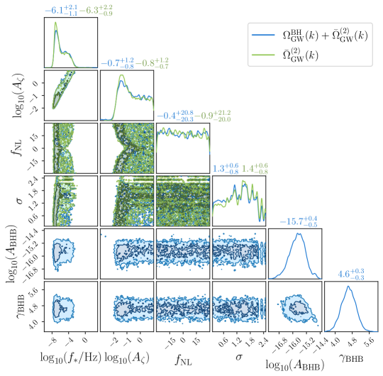
(a) Posterior distributions of $\Omega^{\mathrm{BH}}_{\mathrm{GW}}(k)+\bar{\Omega}^{(2)}_{\mathrm{GW}}(k)$ and $\bar{\Omega}^{(2)}_{\mathrm{GW}}(k)$.

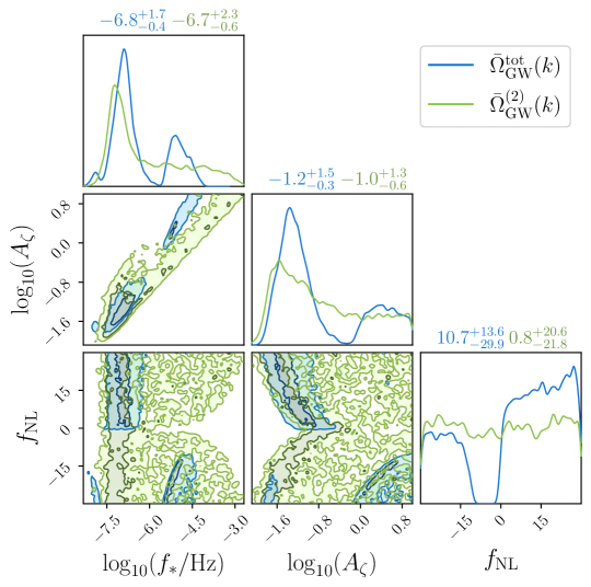
(b) Posterior distributions of $\bar{\Omega}^{(2)}_{\mathrm{GW}}(k)$ and $\bar{\Omega}^{\mathrm{tot}}_{\mathrm{GW}}(k)$.

Figure 1: The corner plot of the posterior distributions. The contours in the off-diagonal panels denote the $68\%$ and $95\%$ credible intervals of the 2D posteriors. The numbers above the figures represent the median values and $1$-$\sigma$ ranges of the parameters. (a): The blue and green solid curves correspond to the second-order SIGW energy spectrum in Eq. (3) with or without SMBHB. (b): The green and blue lines represent the energy density spectra of second-order SIGW in Eq. (3) and the complete one-loop and two-loop energy spectra incorporating up to third-order SIGW in Eq. (10), respectively. We have fixed $\sigma=1$.

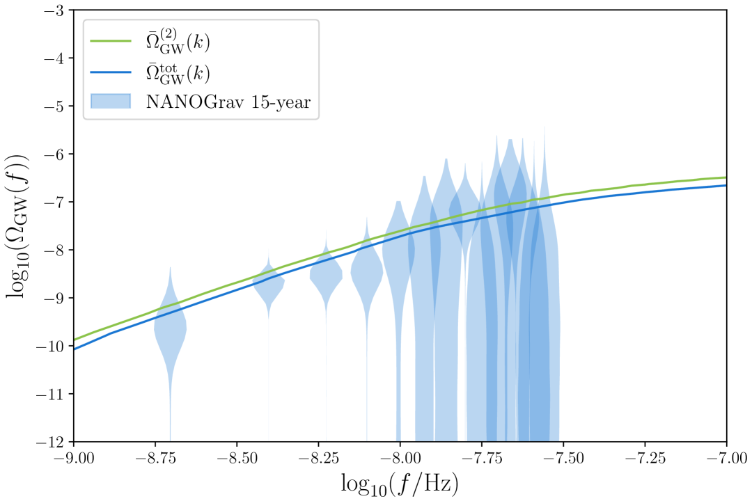
Figure 2: The energy density spectra $\bar{\Omega}^{(2)}_{\mathrm{GW}}(k)$ and $\bar{\Omega}^{\mathrm{tot}}_{\mathrm{GW}}(k)$ correspond to Fig. 1b. The energy density spectra derived from the free spectrum of the NANOGrav 15-year are shown with blue. The green curves represent the energy density spectra of GW with different line styles labeled in the figure. Specifically, the parameters for the blue solid line are: $\log_{10}(A_{\zeta})=-1.51$, $\log_{10}(f_{*}/\mathrm{Hz})=-7.14$, and $f_{\mathrm{NL}}=22.3$; and for the green solid line, the parameters are: $\log_{10}(A_{\zeta})=-1.32$, $\log_{10}(f_{*}/\mathrm{Hz})=-6.991$, and $f_{\mathrm{NL}}=23.4$. These parameters are selected based on the MAP estimate for each parameter.

II.2 SNR of LISA

In scenarios where the high-frequency region of the energy spectrum of SIGW is within detection range of LISA, we can combine PTA observational data to thoroughly analyze the impact of $\mathcal{P}_{\zeta}\left(k\right)$ and $f_{\mathrm{NL}}$ on the SNR of LISA, thereby determining the influence of the high-frequency SIGW on LISA observations. The SNR $\rho$ of LISA is given by Siemens et al. (2013)

$$\rho=\sqrt{T}\left[\int\mathop{}\!\mathrm{d}f\left(\frac{\bar{\Omega}_{\mathrm{GW},0}(f)}{\Omega_{\mathrm{n}}(f)}\right)^{2}\right]^{1/2}\ ,$$ (17)

where $T$ is the observation time and we set $T=4$ years here. $\Omega_{\mathrm{n}}(f)=2\pi^{2}f^{3}S_{n}/3H_{0}^{2}$, where $H_{0}$ is the Hubble constant and $S_{n}$ is the strain noise power spectral density Robson et al. (2019).

As shown in Fig. 3, we provide a two-dimensional distribution plot of SNR of LISA as a function of $\sigma$ and $f_{*}$. The results indicate that when SIGW dominate the current PTA observations, the corresponding energy density spectrum in the high-frequency region can influence observations in the LISA frequency band. Moreover, as elaborated in Sec. III.2, large-amplitude primordial perturbations at small scales can lead to the formation of primordial black holes, while binary PBH mergers also contribute to the SGWB. When SIGW dominate PTA observations, the SGWB produced by binary PBH mergers may also impact GW observations at higher frequencies.

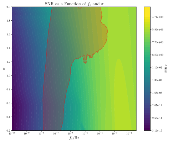
Figure 3: The SNR of LISA as a function of $f_{*}$ and $\sigma$. The heatmap shows the SNR for second-order SIGW energy spectrum $\bar{\Omega}^{(2)}_{\mathrm{GW}}(k)$ with fixed values of $A_{\zeta}=0.1$ and $f_{\mathrm{NL}}=5$. The red shading represents the $68\%$ credible interval corresponding to the two-dimensional posterior distribution of $\bar{\Omega}^{(2)}_{\mathrm{GW}}(k)$ shown in Fig. 1a, obtained using the KDE method implemented in ChainConsumer Hinton (2016); Hinton et al. (2024).

II.3 Constraints from large-scale cosmological observations

Besides the direct observation of the energy density spectrum of SIGW, SIGW can serve as an additional radiation component, affecting the large-scale cosmological observations Zhou et al. (2025); Wright et al. (2024); Ben-Dayan et al. (2019). More precisely, the total energy density of SIGW satisfies

$$h^{2}\rho_{\mathrm{GW}}=\int_{f_{\mathrm{min}}}^{\infty}h^{2}\Omega_{\mathrm{GW},0}(k)\mathop{}\!\mathrm{d}\left(\ln k\right)<2.9\times 10^{-7}$$ (18)

at $95\%$ confidence level for CMB$+$BAO data Clarke et al. (2020). It should be noted that the large-scale cosmological observation constraints in Ref. Clarke et al. (2020) are stronger than the constraints obtained from the relativistic degrees of freedom $N_{\text{eff}}$ in Refs. Wang et al. (2024a); Zhou et al. (2025). More precisely, taking into account only the constraints from $N_{\text{eff}}$, the energy density spectrum of SIGW satisfies $h^{2}\rho_{\mathrm{GW}}<2.11\times 10^{-6}$ at the $95\%$ confidence level, which represents a weaker constraint compared to that provided in Eq. (18). In Fig. 4, we present the parameter space of $\mathcal{P}_{\zeta}(k)$ and $f_{\mathrm{NL}}$ determined by Eq. (18).

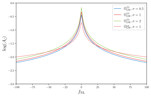
Figure 4: The upper limits of the amplitude of LN primordial power spectrum $A_{\zeta}$ as determined by large-scale observations under different non-Gaussian parameter $f_{\mathrm{NL}}$. The figure illustrates the upper limits of $A_{\zeta}$, as determined by the energy density spectra of Eq. (3) (solid line) and Eq. (10) (dashed line).

As depicted in Fig. 4, the total energy density spectrum of second-order SIGW $\Omega^{(2)}_{\mathrm{GW}}$ in Eq. (3) is proportional to $A_{\zeta}^{2}+(f_{\mathrm{NL}})^{2}A_{\zeta}^{3}+(f_{\mathrm{NL}})^{4}A_{\zeta}^{4}$ , creating a degeneracy for opposite values of $f_{\mathrm{NL}}$ , where the upper limits of $A_{\zeta}$ for $f_{\mathrm{NL}}$ and $-f_{\mathrm{NL}}$ are identical. However, in Eq. (10), where one-loop and two-loop contributions extend to third order, the corresponding energy density spectrum $\Omega^{\mathrm{tot}}_{\mathrm{GW}}$ is proportional to $A_{\zeta}^{2}+A_{\zeta}^{3}+f_{\mathrm{NL}}A_{\zeta}^{3}+(f_{\mathrm{NL}})^{2}A_{\zeta}^{3}$, causing the upper limits of $A_{\zeta}$ to differ for parameters $f_{\mathrm{NL}}$ with equal magnitudes but opposite signs. Furthermore, when $|f_{\mathrm{NL}}|$ is small, the third-order SIGW contribution from Eq. (10) suppresses the upper bound of $A_{\zeta}$. As $|f_{\mathrm{NL}}|$ increases, the three-loop contribution proportional to $(f_{\mathrm{NL}})^{4}A_{\zeta}^{4}$ in Eq. (3) grows, leading to the upper limit of $A_{\zeta}$ from Eq. (3) becoming lower than that from Eq. (10).

III Primordial black holes

On small scales, large-amplitude primordial curvature perturbations can generate SIGW upon re-entering the horizon after inflation. This process is inevitably accompanied by the formation of PBH. In this section, we consider PBH formed from large-amplitude primordial curvature perturbations on small scales, and the constraints they impose on the small-scale primordial power spectrum and primordial non-Gaussianity. Furthermore, binary PBH mergers will also generate an additional SGWB Wang et al. (2019). By combining the results of SIGW from the previous section, we analyze the impact of binary PBH mergers on the observations of SGWB.

III.1 Abundance of PBH

The abundance of PBH can be expressed as Sasaki et al. (2018)

$$f_{\mathrm{pbh}}\simeq 2.5\times 10^{8}\beta\left(\frac{g_{*}^{\text{form }}}{10.75}\right)^{-\frac{1}{4}}\left(\frac{m_{\mathrm{pbh}}}{M_{\odot}}\right)^{-\frac{1}{2}}\ .$$ (19)

We consider an approximate formula for $f_{\mathrm{PBH}}$ in Eq. (19). The corresponding rigorous expressions are provided in Refs. Ferrante et al. (2023); Iovino et al. (2024); Franciolini et al. (2023). The mass of PBH is characterised by the scaling law relation

$$M_{\mathrm{PBH}}=\mathcal{K}M_{H}\left(\mathcal{C}-\mathcal{C}_{\mathrm{th}}\right)^{\gamma}\ ,$$ (20)

$$M_{H}\approx 7M_{\odot}\left(\frac{k}{10^{6}\mathrm{Mpc}^{-1}}\right)^{-2}\left(\frac{g_{*}}{10.75}\right)^{-1/6}\ ,$$

where the threshold $\mathcal{C}_{\text{th}}$ have been studied in Ref. Musco et al. (2021). The compaction function $\mathcal{C}=\mathcal{C}_{1}-\mathcal{C}_{1}^{2}/(4\Phi)$ can be obtained from the linear $\mathcal{C}_{1}=\mathcal{C}_{\mathrm{G}}\mathop{}\!\mathrm{d}F/\mathop{}\!\mathrm{d}\zeta_{\mathrm{G}}$ component, that uses $\mathcal{C}_{\mathrm{G}}=$ $-2\Phi r\zeta_{G}^{\prime}$, where $\Phi=3(1+w)/(5+3w)$. In the case of local-type primordial non-Gaussianity, $F\left(\zeta_{\mathrm{G}}\right)=\zeta_{\mathrm{G}}+\frac{3}{5}f_{\mathrm{NL}}\zeta_{\mathrm{G}}^{2}$. We set $\mathcal{K}=4.4$ and $\gamma=0.38$ Musco et al. (2024); Iovino et al. (2024). The mass fraction $\beta$ can be obtained by integrating the probability distribution function

$$\beta=\int_{\mathcal{D}}\mathcal{K}\left(\mathcal{C}-\mathcal{C}_{\mathrm{th}}\right)^{\gamma}\mathrm{P}_{\mathrm{G}}\left(\mathcal{C}_{\mathrm{G}},\zeta_{\mathrm{G}}\right)\mathop{}\!\mathrm{d}\mathcal{C}_{\mathrm{G}}\mathop{}\!\mathrm{d}\zeta_{\mathrm{G}}\ ,$$ (21)

where the domain of integration in Eq. (21) is $\mathcal{D}=$ $\left\{\mathcal{C}\left(\mathcal{C}_{\mathrm{G}},\zeta_{\mathrm{G}}\right)>\mathcal{C}_{\text{th}}\wedge\mathcal{C}_{1}\left(\mathcal{C}_{\mathrm{G}},\zeta_{\mathrm{G}}\right)<2\Phi\right\}$. In Eq. (21), the Gaussian components are distributed as

$$P_{\mathrm{G}}\left(\mathcal{C}_{\mathrm{G}},\zeta_{\mathrm{G}}\right)=\frac{e^{\left[-\frac{1}{2\left(1-\gamma_{cr}^{2}\right)}\left(\frac{\mathcal{C}_{\mathrm{G}}}{\sigma_{c}}-\frac{\gamma_{cr}\zeta_{\mathrm{G}}}{\sigma_{r}}\right)^{2}-\frac{\zeta_{\mathrm{G}}^{2}}{2\sigma_{r}^{2}}\right]}}{2\pi\sigma_{c}\sigma_{r}\sqrt{1-\gamma_{cr}^{2}}}\ .$$ (22)

The correlators in Eq. (22) are given by

$$\sigma_{c}^{2}=\frac{4\Phi^{2}}{9}\int_{0}^{\infty}\frac{\mathop{}\!\mathrm{d}k}{k}\left(kr_{m}\right)^{4}W^{2}\left(k,r_{m}\right)P_{\zeta}^{T}\ ,$$ (23)

$$\sigma_{cr}^{2}=\frac{2\Phi}{3}\int_{0}^{\infty}\frac{\mathop{}\!\mathrm{d}k}{k}\left(kr_{m}\right)^{2}W\left(k,r_{m}\right)W_{s}\left(k,r_{m}\right)P_{\zeta}^{T}\ ,$$

$$\sigma_{r}^{2}=\int_{0}^{\infty}\frac{\mathop{}\!\mathrm{d}k}{k}W_{s}^{2}\left(k,r_{m}\right)P_{\zeta}^{T}\ ,$$

where $P_{\zeta}^{T}=T^{2}\left(k,r_{m}\right)P_{\zeta}(k)$, and $\gamma_{cr}\equiv\sigma_{cr}^{2}/\sigma_{c}\sigma_{r}$. Here, we have defined $W\left(k,r_{m}\right),W_{s}\left(k,r_{m}\right)$ and $T\left(k,r_{m}\right)$ as the top-hat window function, the spherical-shell window function, and the radiation transfer function Young (2022). It is important to note that the calculation of PBH abundance is highly model-dependent, and different models can lead to significant variations in the estimated abundance Iovino et al. (2024).

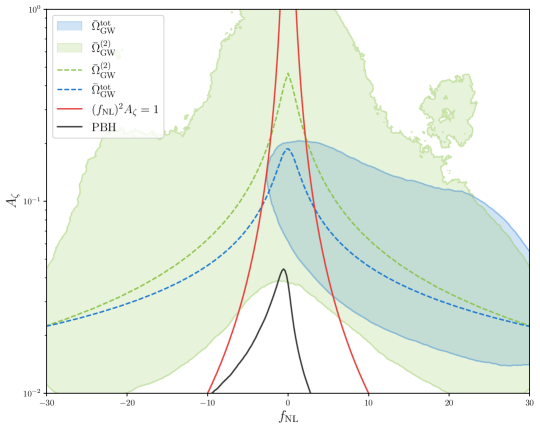
Figure 5: The constraints on $A_{\zeta}$ and $f_{\mathrm{NL}}$ assuming the LN primordial power spectrum. The blue and green shaded regions represent the $68\%$ credible intervals corresponding to the two-dimensional posterior distribution shown in Fig. 1b with the KDE method. The blue and green dashed lines indicate the upper bounds on the amplitude $A_{\zeta}$ shown in Fig. 4. The red curve corresponds to the relation $(f_{\mathrm{NL}})^{2}A_{\zeta}=1$. The black line corresponds to the PBH abundance constraint given in Ref. Carr et al. (2021).

As shown in Fig. 5, we present the constraints on the amplitude of the small-scale primordial power spectrum $A_{\zeta}$ and the primordial non-Gaussian parameter $f_{\mathrm{NL}}$ in the case of the LN primordial power spectrum, based on current CMB$+$BAO$+$PTA$+$PBH observations. Furthermore, in the case of local-type primordial non-Gaussianity, the second-order energy density $\bar{\Omega}^{(2)}_{\mathrm{GW}}$ is proportional to $A_{\zeta}^{2}+(f_{\mathrm{NL}})^{2}A_{\zeta}^{3}+(f_{\mathrm{NL}})^{4}A_{\zeta}^{4}$ , and each increase in the non-Gaussian order introduces an additional perturbative expansion coefficient $(f_{\mathrm{NL}})^{2}A_{\zeta}$. This result holds for $n$-th order SIGW, such that: $\bar{\Omega}^{(n)}_{\mathrm{GW}}\sim A_{\zeta}^{n}\sum_{m=0}^{n}(f_{\mathrm{NL}})^{2m}A_{\zeta}^{m}$. Therefore, the necessary condition for ensuring the convergence of the perturbative expansion of non-Gaussian contributions is $(f_{\mathrm{NL}})^{2}A_{\zeta}<1$. This theoretical constraint corresponds to the region below the red curve in Fig. 5.

Through various types of cosmological observations across different scales, we can effectively constrain the primordial non-Gaussian parameter $f_{\mathrm{NL}}$ on small scales. It is important to note that these constraints depend on the specific form of the small-scale primordial power spectrum. In Sec. IV, we will analyze the impact of different primordial power spectra on the constraints of the parameter $f_{\mathrm{NL}}$. Additionally, the parameter space shown in Fig. 5 is influenced by experimental observations, and future high-precision cosmological measurements will further refine our ability to constrain small-scale primordial non-Gaussian parameter.

III.2 SGWB from binary PBH mergers

In Sec. II.2, we investigated how SIGW influence the SNR of LISA. As we previously mentioned, when SIGW dominate PTA observations, their generation inevitably accompanies the formation of PBH, and binary PBH mergers also contribute to the SGWB. In this paper, we follow the formation scenario of PBH binaries proposed in Refs. Wang et al. (2018); Sasaki et al. (2016); Abbott et al. (2018). Based on the merger rate of the PBH binaries, we can calculate the energy density spectra $\Omega_{\mathrm{GW}}^{\mathrm{PBH}}(f)$ of the corresponding SGWB. For the SGWB produced by binary PBH mergers, $\Omega_{\mathrm{GW}}^{\mathrm{PBH}}(f)$ can be expressed as

$$\Omega_{\mathrm{GW}}^{\mathrm{PBH}}(f)=\frac{\nu}{\rho_{\mathrm{c}}}\int_{0}^{\frac{f_{\mathrm{cut}}}{f}-1}\frac{R_{\mathrm{PBH}}(z)}{(1+z)H(z)}\frac{\mathop{}\!\mathrm{d}E_{\mathrm{GW}}}{\mathop{}\!\mathrm{d}f_{\mathrm{s}}}\left(f_{\mathrm{s}}\right)\mathop{}\!\mathrm{d}z\ ,$$ (24)

where the explicit expressions of $\frac{\mathop{}\!\mathrm{d}E_{\mathrm{GW}}}{\mathop{}\!\mathrm{d}f_{\mathrm{s}}}\left(f_{\mathrm{s}}\right)$ and $R_{\mathrm{PBH}}(z)$ can be found in Ref. Wang et al. (2019). As shown in Fig. 6, when SIGW lie within the observational frequency range of PTA, the SGWB generated by the corresponding binary PBH mergers falls within LISA’s detection frequency band, which may affect the SNR of LISA.

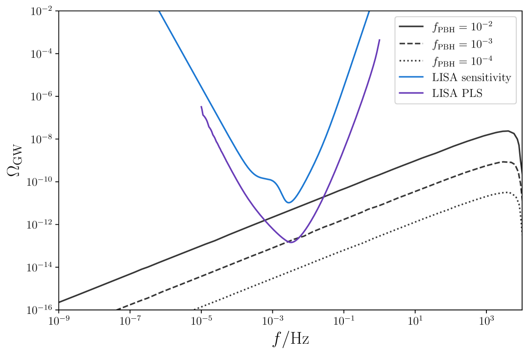
Figure 6: The energy density spectrum $\bar{\Omega}^{\mathrm{PBH}}_{\mathrm{GW}}(k)$ in Eq. (24). The black curves represent the energy spectra of ${\Omega}^{\mathrm{PBH}}_{\mathrm{GW}}(k)$ with $M_{\mathrm{PBH}}=1M_{\odot}$ and $f_{\mathrm{PBH}}=10^{-2}$ (solid), $10^{-3}$ (dashed) and $10^{-4}$ (dotted) Kohri and Terada (2021). The blue curve and the purple curve represent the stardand LISA sensitivity and the PLS Babak et al. (2021) with SNR $=10$.

IV Shape of the primordial power spectra

In the above discussion, we have provided the constraints on the local-type non-Gaussian parameter $f_{\mathrm{NL}}$ from current cosmological observations for a LN primordial power spectrum. This result depends on the specific form of the primordial power spectrum. To study the effects of different shapes of the primordial power spectrum on small-scale cosmological observations, we need to combine current PTA observational data and analyze the Bayes factors of different primordial power spectra. Besides the previously analyzed LN primordial power spectrum, we consider the BPL primordial power spectrum You et al. (2023); Byrnes et al. (2019)

$$\mathcal{P}_{\zeta}^{\mathrm{BPL}}(k)=\frac{A_{\zeta}(\alpha+\beta)}{\left(\beta\left(k/k_{*}\right)^{-\alpha}+\alpha\left(k/k_{*}\right)^{\beta}\right)}\ ,$$ (25)

and the $\delta$ (monochromatic) primordial power spectrum Peng et al. (2021); Zhou et al. (2020); Cai et al. (2018)

$$\mathcal{P}_{\zeta}^{\delta}(k)=A_{\zeta}k_{*}\delta\left(k-k_{*}\right)\ .$$ (26)

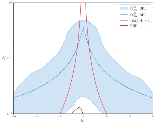
(a) The constraints on $A_{\zeta}$ and $f_{\mathrm{NL}}$ assuming the BPL primordial power spectrum..

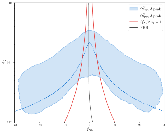
(b) The constraints on $A_{\zeta}$ and $f_{\mathrm{NL}}$ assuming the monochromatic primordial power spectrum.

Figure 7: The constraints on $A_{\zeta}$ and $f_{\mathrm{NL}}$ assuming different primordial power spectrum. The blue shaded regions represent the $68\%$ credible intervals corresponding to the two-dimensional posterior distribution with KDE method. The blue dashed lines indicate the upper bounds on the amplitude $A_{\zeta}$ from CMB$+$BAO data. The red curve corresponds to the relation $(f_{\mathrm{NL}})^{2}A_{\zeta}=1$. The black line corresponds to the PBH abundance constraint given in Ref. Carr et al. (2021). As stated in Ref. Ferrante et al. (2023), Eq. (21) is not applicable to a monochromatic primordial power spectrum. Therefore, we adopt the approach proposed in Ref. Byrnes et al. (2012) to calculate the PBH abundance under the monochromatic primordial power spectrum scenario.

Similar to the discussions in Sec. II and Sec. III, the constraints imposed by current cosmological observations on the parameter space of the BPL primordial power spectrum and the monochromatic primordial power spectrum are presented in Fig. 7a and Fig. 7b, respectively. The corresponding posterior distributions are given in the Appendix. A. For the monochromatic power spectrum, the prior distributions of $\log(f_{*}/\mathrm{Hz})$, $\log(A_{\zeta})$, and $f_{\mathrm{NL}}$ are uniformly distributed over the ranges $[-10,-5]$, $[-3,0]$, and $[-30,30]$ respectively. For the BPL power spectrum, the prior distributions of $\log(f_{*}/\mathrm{Hz})$, $\log(A_{\zeta})$, $\alpha$, $\beta$ and $f_{\mathrm{NL}}$ are uniformly distributed over the ranges $[-10,-5]$, $[-3,0]$, $[1,3]$, $[1,3]$,and $[-30,30]$ respectively.

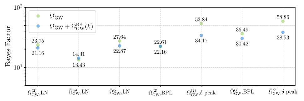
Figure 8: The Bayes factors between different models. The vertical axis represents the Bayes factor of different models relative to SMBHB, and the horizontal axis represents the different models. The green dots are for models without SMBHB and the blue dots are for models in combination with the SMBHB signal.

To rigorously quantify the probability of different models dominating current PTA observations, we employ the Bayes factor to compare them. Specifically, the Bayes factor is defined as $B_{i,j}=\frac{Z_{i}}{Z_{j}}$, where $Z_{i}$ represents the evidence of model $H_{i}$. Fig. 8 illustrates Bayes factors for comparisons between various models and the SMBHB model. As shown in Fig. 8, the Bayes factor analysis indicates that SIGW generated by the monochromatic primordial power spectrum are more likely to dominate the current PTA observations.

In Table. 1, we summarize the main results of this section. The observational constraints on the parameter of small-scale primordial non-Gaussianity $f_{\mathrm{NL}}$ depend not only on the specific form of the primordial power spectrum but also on its amplitude $A_{\zeta}$. In Table. 1, we have set $A_{\zeta}=10^{-2}$. Note that the above conclusion differs from the constraints on $f_{\mathrm{NL}}$ at large scales, as the primordial power spectrum at large scales has already been strictly constrained by large-scale cosmological observations. Therefore, different forms of the primordial power spectrum do not need to be considered when determining the constraints on $f_{\mathrm{NL}}$ at large scales.

Furthermore, if no specific assumption is made about the origin of the SGWB in the PTA frequency band, the energy density spectrum of second-order SIGW must not exceed the observed energy density spectrum in the PTA band. In this scenario, current PTA observations can still serve as an upper bound on the energy density spectrum of second-order SIGW. Thus, when we require SIGW to dominate the current PTA observations, the parameter space of $f_{\mathrm{NL}}$ and $A_{\zeta}$ must not only satisfy other cosmological constraints but also lie within the blue-shaded regions in Fig. 7a and Fig. 7b. Since $\bar{\Omega}^{(2)}_{\mathrm{GW}}(k)$ increases with $f_{\mathrm{NL}}$ and $A_{\zeta}$, if we do not assume that SIGW dominate the SGWB in the PTA frequency band, then the value of $A_{\zeta}$ for a given $f_{\mathrm{NL}}$ must not exceed the blue-shaded regions in Fig. 7a and Fig. 7b.

	$f_{\mathrm{NL}}$	Bayes factors
LN	$-9.5<f_{\mathrm{NL}}<2.9$	23.75
BPL	$-5.0<f_{\mathrm{NL}}<-0.1$	22.61
$\delta$ peak	$-10.0<f_{\mathrm{NL}}<1.2$	53.84
SMBHB	$\times$	1

Table 1: Constraints from current cosmological observations on small-scale local-type non-Gaussian parameters. We set $A_{\zeta}=1$.

Moreover, as discussed in Sec. II, the cross-correlation function $\langle h^{\lambda,(3)}_{\mathbf{k}}h^{\lambda^{\prime},(2)}_{\mathbf{k}^{\prime}}\rangle\sim f_{\mathrm{NL}}A_{\zeta}^{3}$ can impact the results in Table. 1. When constraining the parameter $f_{\mathrm{NL}}$ using the energy density spectrum in Eq. (10), the current PTA observations cannot be dominated by SIGW. As indicated by the blue shaded region in Fig. 5, the presence of the cross-correlation function $\langle h^{\lambda,(3)}_{\mathbf{k}}h^{\lambda^{\prime},(2)}_{\mathbf{k}^{\prime}}\rangle$ suppresses the total energy density spectrum of SIGW when $f_{\mathrm{NL}}$ is negative, thus excluding certain parameter regions based on cosmological constraints. In this scenario, insisting that SIGW dominate the current PTA observations would contradict the upper bound on the primordial black hole abundance.

V Conclusion and discussion

To study the constraints imposed by current cosmological observations on the small-scale primordial power spectrum $\mathcal{P}_{\zeta}\left(k\right)$ and the local-type non-Gaussian parameter $f_{\mathrm{NL}}$, we analyzed the impact of large-amplitude small-scale primordial curvature perturbations, which induce the formation of PBH and corresponding second-order SIGW, on current cosmological observations at different scales. Future, more precise observations from PTA, PBH, and large-scale cosmological observations will enable us to more tightly constrain the parameter space of $\mathcal{P}_{\zeta}\left(k\right)$ and $f_{\mathrm{NL}}$. Furthermore, since SIGW and PBH abundance depend on the shape of the primordial power spectrum, we studied the impact of different primordial power spectra on the constraints of the parameter space and rigorously analyzed the Bayes factors of different models. Moreover, the constraints on $f_{\mathrm{NL}}$ imposed by current cosmological observations for different forms of the primordial power spectrum are summarized in Table 1. The constraints on $f_{\mathrm{NL}}$ presented in Table. 1 depend on the specific form and the amplitude of the primordial power spectra.

In this study, we evaluated the influence of second-order and third-order SIGW on current cosmological observations. As shown in Refs. De Luca et al. (2023); Nakama and Suyama (2015); Chang et al. (2024c); Nakama and Suyama (2016); Zhou et al. (2023), second-order density perturbations induced by primordial perturbations will have a significant impact on the threshold $\delta_{c}$ and probability distribution function $P\left(\delta\right)$ of PBH. When studying the large-amplitude primordial perturbations on small scales, the effects of higher-order cosmological perturbations cannot be ignored Zhou et al. (2024). In addition to the influence of higher-order corrections, several other effects could impact the parameter space of $\mathcal{P}_{\zeta}\left(k\right)$ and $f_{\mathrm{NL}}$. These include the effects of different dominant era of universe Chen et al. (2024); Balaji et al. (2023); Zhu et al. (2024), the impact of large-amplitude small-scale primordial tensor perturbations Chang et al. (2023b); Bari et al. (2024); Yu and Wang (2024); Picard and Davies (2024); Picard and Malik (2024), and interactions between SIGW and matter Saga et al. (2015); Zhang et al. (2022); Yu and Wang (2025); Sui et al. (2024). The impact of these physical effects on the constraints of primordial non-Gaussianity might be systematically investigated in future research.

Appendix A Posterior distributions

Based on the theoretical results of the energy density spectrum of second-orderSIGW, we present the posterior distributions determined by current PTA observations under different forms of the primordial power spectrum. As shown in Fig. 8, we further analyze the impact of SIGW on PTA observations when $f_{\mathrm{NL}}=0$. The posterior distributions for different models are provided in Fig. 9 $\sim$ Fig. 14.

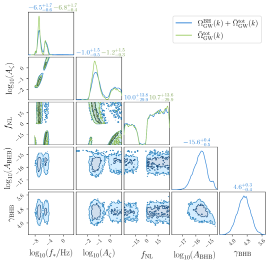
Figure 9: Posterior distributions of $\bar{\Omega}^{\mathrm{tot}}_{\mathrm{GW}}(k)$ and $\bar{\Omega}^{\mathrm{BH}}_{\mathrm{GW}}(k)+\bar{\Omega}^{\mathrm{tot}}_{\mathrm{GW}}(k)$ with LN primordial power spectrum. The contours in the off-diagonal panels denote the $68\%$ and $95\%$ credible intervals of the 2D posteriors. The numbers above the figures represent the median values and $1$-$\sigma$ ranges of the parameters.

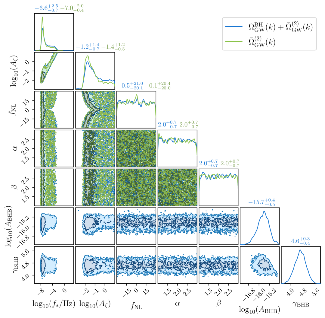
Figure 10: Posterior distributions of $\bar{\Omega}^{(2)}_{\mathrm{GW}}(k)$ and $\bar{\Omega}^{\mathrm{BH}}_{\mathrm{GW}}(k)+\bar{\Omega}^{(2)}_{\mathrm{GW}}(k)$ with BPL primordial power spectrum. The contours in the off-diagonal panels denote the $68\%$ and $95\%$ credible intervals of the 2D posteriors. The numbers above the figures represent the median values and $1$-$\sigma$ ranges of the parameters.

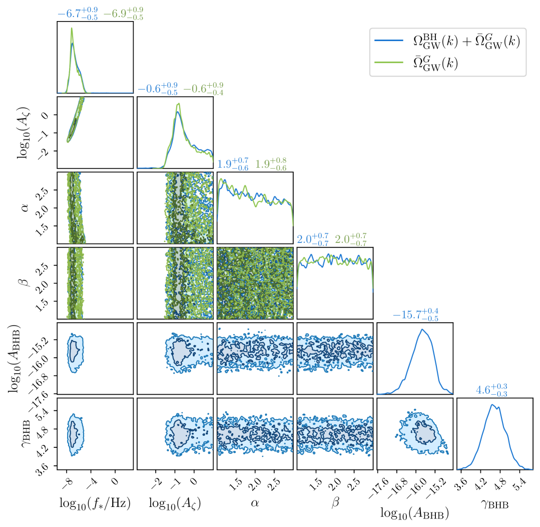
Figure 11: Posterior distributions of $\bar{\Omega}^{G}_{\mathrm{GW}}(k)$ and $\bar{\Omega}^{\mathrm{BH}}_{\mathrm{GW}}(k)+\bar{\Omega}^{G}_{\mathrm{GW}}(k)$ with BPL primordial power spectrum. The contours in the off-diagonal panels denote the $68\%$ and $95\%$ credible intervals of the 2D posteriors. The numbers above the figures represent the median values and $1$-$\sigma$ ranges of the parameters.

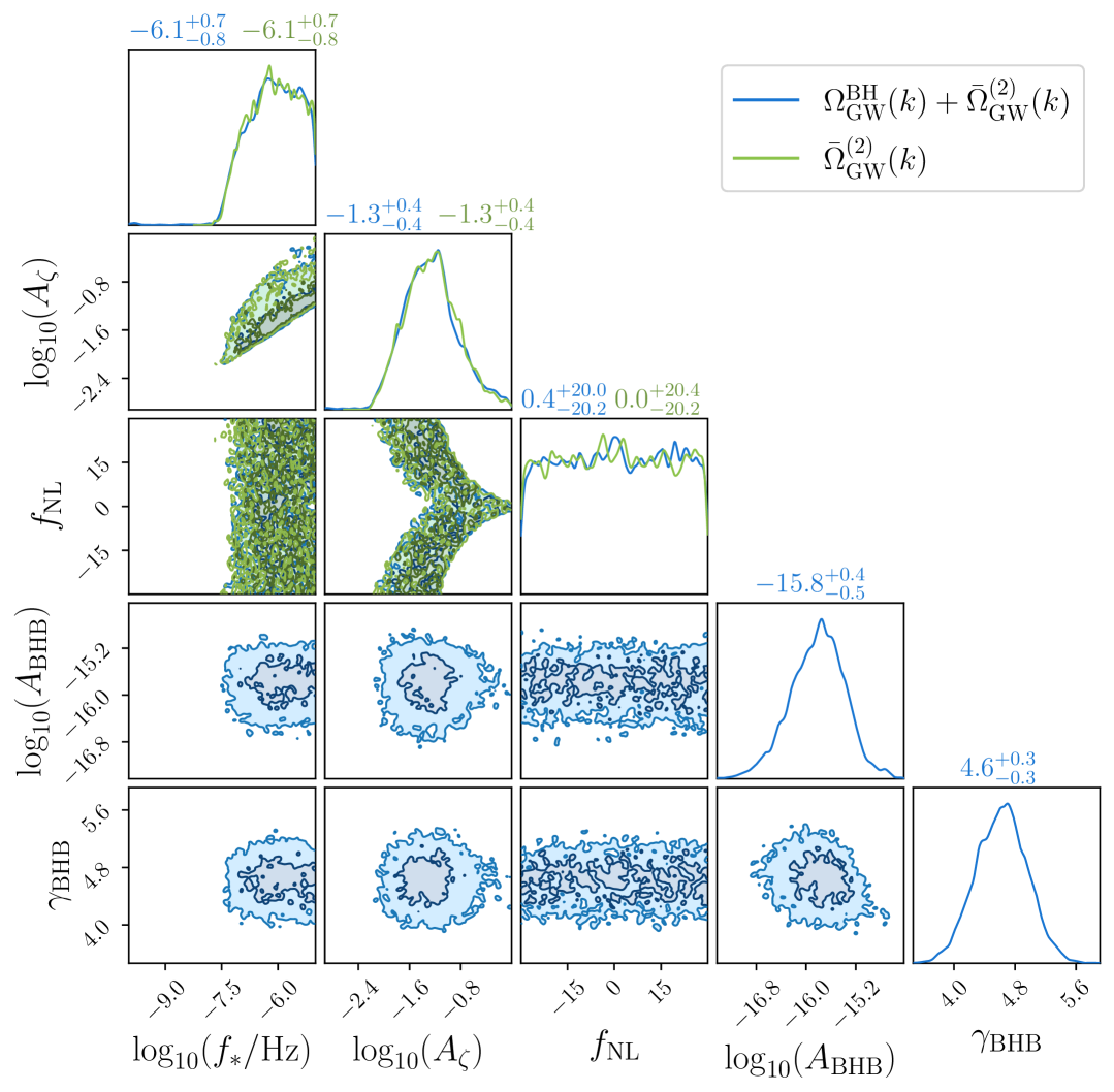
Figure 12: Posterior distributions of $\bar{\Omega}^{(2)}_{\mathrm{GW}}(k)$ and $\bar{\Omega}^{\mathrm{BH}}_{\mathrm{GW}}(k)+\bar{\Omega}^{(2)}_{\mathrm{GW}}(k)$ with monochromatic primordial power spectrum. The contours in the off-diagonal panels denote the $68\%$ and $95\%$ credible intervals of the 2D posteriors. The numbers above the figures represent the median values and $1$-$\sigma$ ranges of the parameters.

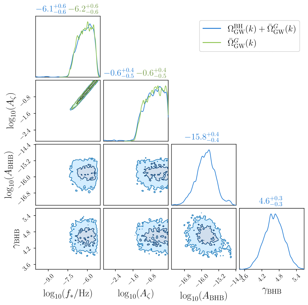
Figure 13: Posterior distributions of $\bar{\Omega}^{G}_{\mathrm{GW}}(k)$ and $\bar{\Omega}^{\mathrm{BH}}_{\mathrm{GW}}(k)+\bar{\Omega}^{G}_{\mathrm{GW}}(k)$ with monochromatic primordial power spectrum. The contours in the off-diagonal panels denote the $68\%$ and $95\%$ credible intervals of the 2D posteriors. The numbers above the figures represent the median values and $1$-$\sigma$ ranges of the parameters.

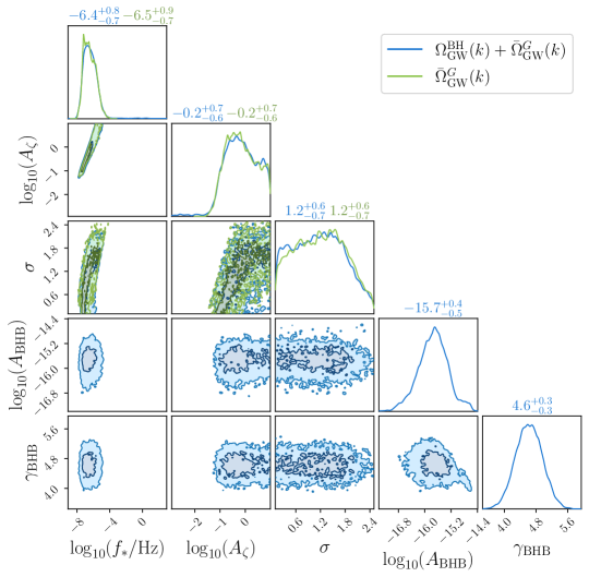
Figure 14: Posterior distributions of $\bar{\Omega}^{G}_{\mathrm{GW}}(k)$ and $\bar{\Omega}^{\mathrm{BH}}_{\mathrm{GW}}(k)+\bar{\Omega}^{G}_{\mathrm{GW}}(k)$ with LN primordial power spectrum. The contours in the off-diagonal panels denote the $68\%$ and $95\%$ credible intervals of the 2D posteriors. The numbers above the figures represent the median values and $1$-$\sigma$ ranges of the parameters.

References

- Lyth and Rodriguez (2005) D. H. Lyth and Y. Rodriguez, Phys. Rev. Lett. 95, 121302 (2005), arXiv:astro-ph/0504045 .
- Weinberg (2005) S. Weinberg, Phys. Rev. D 72, 043514 (2005), arXiv:hep-th/0506236 .
- Bassett et al. (2006) B. A. Bassett, S. Tsujikawa, and D. Wands, Rev. Mod. Phys. 78, 537 (2006), arXiv:astro-ph/0507632 .
- Baumann (2011) D. Baumann, in Theoretical Advanced Study Institute in Elementary Particle Physics: Physics of the Large and the Small (2011) pp. 523–686, arXiv:0907.5424 [hep-th] .
- Riotto (2003) A. Riotto, ICTP Lect. Notes Ser. 14, 317 (2003), arXiv:hep-ph/0210162 .
- Goldwirth and Piran (1992) D. S. Goldwirth and T. Piran, Phys. Rept. 214, 223 (1992).
- Malik and Wands (2009) K. A. Malik and D. Wands, Phys. Rept. 475, 1 (2009), arXiv:0809.4944 [astro-ph] .
- Baumann (2018) D. Baumann, PoS TASI2017, 009 (2018), arXiv:1807.03098 [hep-th] .
- Irastorza and Redondo (2018) I. G. Irastorza and J. Redondo, Prog. Part. Nucl. Phys. 102, 89 (2018), arXiv:1801.08127 [hep-ph] .
- Cai et al. (2016) Y.-F. Cai, S. Capozziello, M. De Laurentis, and E. N. Saridakis, Rept. Prog. Phys. 79, 106901 (2016), arXiv:1511.07586 [gr-qc] .
- Marsh (2016) D. J. E. Marsh, Phys. Rept. 643, 1 (2016), arXiv:1510.07633 [astro-ph.CO] .
- De Felice and Tsujikawa (2010) A. De Felice and S. Tsujikawa, Living Rev. Rel. 13, 3 (2010), arXiv:1002.4928 [gr-qc] .
- Bojowald (2005) M. Bojowald, Living Rev. Rel. 8, 11 (2005), arXiv:gr-qc/0601085 .
- Gasperini and Veneziano (2003) M. Gasperini and G. Veneziano, Phys. Rept. 373, 1 (2003), arXiv:hep-th/0207130 .
- Lyth and Riotto (1999) D. H. Lyth and A. Riotto, Phys. Rept. 314, 1 (1999), arXiv:hep-ph/9807278 .
- Kim and Carosi (2010) J. E. Kim and G. Carosi, Rev. Mod. Phys. 82, 557 (2010), [Erratum: Rev.Mod.Phys. 91, 049902 (2019)], arXiv:0807.3125 [hep-ph] .
- Abdalla et al. (2022) E. Abdalla et al., JHEAp 34, 49 (2022), arXiv:2203.06142 [astro-ph.CO] .
- Workman et al. (2022) R. L. Workman et al. (Particle Data Group), PTEP 2022, 083C01 (2022).
- Navas et al. (2024) S. Navas et al. (Particle Data Group), Phys. Rev. D 110, 030001 (2024).
- Bernardeau et al. (2002) F. Bernardeau, S. Colombi, E. Gaztanaga, and R. Scoccimarro, Phys. Rept. 367, 1 (2002), arXiv:astro-ph/0112551 .
- Bartolo et al. (2004) N. Bartolo, E. Komatsu, S. Matarrese, and A. Riotto, Phys. Rept. 402, 103 (2004), arXiv:astro-ph/0406398 .
- Ade et al. (2014) P. A. R. Ade et al. (Planck), Astron. Astrophys. 571, A24 (2014), arXiv:1303.5084 [astro-ph.CO] .
- Ade et al. (2016) P. A. R. Ade et al. (Planck), Astron. Astrophys. 594, A17 (2016), arXiv:1502.01592 [astro-ph.CO] .
- Dawson et al. (2016) K. S. Dawson et al. (eBOSS), Astron. J. 151, 44 (2016), arXiv:1508.04473 [astro-ph.CO] .
- Aghanim et al. (2020a) N. Aghanim et al. (Planck), Astron. Astrophys. 641, A1 (2020a), arXiv:1807.06205 [astro-ph.CO] .
- Achucarro et al. (2011) A. Achucarro, J.-O. Gong, S. Hardeman, G. A. Palma, and S. P. Patil, JCAP 01, 030 (2011), arXiv:1010.3693 [hep-ph] .
- Aghanim et al. (2020b) N. Aghanim et al. (Planck), Astron. Astrophys. 641, A6 (2020b), [Erratum: Astron.Astrophys. 652, C4 (2021)], arXiv:1807.06209 [astro-ph.CO] .
- Akrami et al. (2020a) Y. Akrami et al. (Planck), Astron. Astrophys. 641, A10 (2020a), arXiv:1807.06211 [astro-ph.CO] .
- Akrami et al. (2020b) Y. Akrami et al. (Planck), Astron. Astrophys. 641, A9 (2020b), arXiv:1905.05697 [astro-ph.CO] .
- Bringmann et al. (2012) T. Bringmann, P. Scott, and Y. Akrami, Phys. Rev. D 85, 125027 (2012), arXiv:1110.2484 [astro-ph.CO] .
- Kristiano and Yokoyama (2024) J. Kristiano and J. Yokoyama, Phys. Rev. Lett. 132, 221003 (2024), arXiv:2211.03395 [hep-th] .
- Ballesteros and Taoso (2018) G. Ballesteros and M. Taoso, Phys. Rev. D 97, 023501 (2018), arXiv:1709.05565 [hep-ph] .
- Braglia et al. (2020) M. Braglia, D. K. Hazra, F. Finelli, G. F. Smoot, L. Sriramkumar, and A. A. Starobinsky, JCAP 08, 001 (2020), arXiv:2005.02895 [astro-ph.CO] .
- Palma et al. (2020) G. A. Palma, S. Sypsas, and C. Zenteno, Phys. Rev. Lett. 125, 121301 (2020), arXiv:2004.06106 [astro-ph.CO] .
- Ballesteros et al. (2020) G. Ballesteros, J. Rey, M. Taoso, and A. Urbano, JCAP 07, 025 (2020), arXiv:2001.08220 [astro-ph.CO] .
- Atal et al. (2020) V. Atal, J. Cid, A. Escrivà, and J. Garriga, JCAP 05, 022 (2020), arXiv:1908.11357 [astro-ph.CO] .
- Pi et al. (2018) S. Pi, Y.-l. Zhang, Q.-G. Huang, and M. Sasaki, JCAP 05, 042 (2018), arXiv:1712.09896 [astro-ph.CO] .
- Kawai and Kim (2021) S. Kawai and J. Kim, Phys. Rev. D 104, 083545 (2021), arXiv:2108.01340 [astro-ph.CO] .
- Lin et al. (2020) J. Lin, Q. Gao, Y. Gong, Y. Lu, C. Zhang, and F. Zhang, Phys. Rev. D 101, 103515 (2020), arXiv:2001.05909 [gr-qc] .
- Arya et al. (2024) R. Arya, R. K. Jain, and A. K. Mishra, JCAP 02, 034 (2024), arXiv:2302.08940 [astro-ph.CO] .
- Bamba and Odintsov (2015) K. Bamba and S. D. Odintsov, Symmetry 7, 220 (2015), arXiv:1503.00442 [hep-th] .
- Chen and Gao (2025) P.-B. Chen and T.-J. Gao, (2025), arXiv:2501.12242 [astro-ph.CO] .
- Peng et al. (2022) Z.-Z. Peng, Z.-M. Zeng, C. Fu, and Z.-K. Guo, Phys. Rev. D 106, 124044 (2022), arXiv:2209.10374 [gr-qc] .
- Khlopov (2010) M. Y. Khlopov, Res. Astron. Astrophys. 10, 495 (2010), arXiv:0801.0116 [astro-ph] .
- Carr et al. (2016) B. Carr, F. Kuhnel, and M. Sandstad, Phys. Rev. D 94, 083504 (2016), arXiv:1607.06077 [astro-ph.CO] .
- Sasaki et al. (2018) M. Sasaki, T. Suyama, T. Tanaka, and S. Yokoyama, Class. Quant. Grav. 35, 063001 (2018), arXiv:1801.05235 [astro-ph.CO] .
- Carr and Kuhnel (2020) B. Carr and F. Kuhnel, Ann. Rev. Nucl. Part. Sci. 70, 355 (2020), arXiv:2006.02838 [astro-ph.CO] .
- De Luca et al. (2021) V. De Luca, G. Franciolini, and A. Riotto, Phys. Rev. Lett. 126, 041303 (2021), arXiv:2009.08268 [astro-ph.CO] .
- Musco (2019) I. Musco, Phys. Rev. D 100, 123524 (2019), arXiv:1809.02127 [gr-qc] .
- Carr et al. (2024) B. Carr, S. Clesse, J. Garcia-Bellido, M. Hawkins, and F. Kuhnel, Phys. Rept. 1054, 1 (2024), arXiv:2306.03903 [astro-ph.CO] .
- Carr and Kuhnel (2022) B. Carr and F. Kuhnel, SciPost Phys. Lect. Notes 48, 1 (2022), arXiv:2110.02821 [astro-ph.CO] .
- Liu et al. (2022) J. Liu, L. Bian, R.-G. Cai, Z.-K. Guo, and S.-J. Wang, Phys. Rev. D 105, L021303 (2022), arXiv:2106.05637 [astro-ph.CO] .
- Choudhury et al. (2023) S. Choudhury, S. Panda, and M. Sami, JCAP 11, 066 (2023), arXiv:2303.06066 [astro-ph.CO] .
- Gouttenoire and Volansky (2024) Y. Gouttenoire and T. Volansky, Phys. Rev. D 110, 043514 (2024), arXiv:2305.04942 [hep-ph] .
- Belotsky et al. (2014) K. M. Belotsky, A. D. Dmitriev, E. A. Esipova, V. A. Gani, A. V. Grobov, M. Y. Khlopov, A. A. Kirillov, S. G. Rubin, and I. V. Svadkovsky, Mod. Phys. Lett. A 29, 1440005 (2014), arXiv:1410.0203 [astro-ph.CO] .
- Domènech (2021) G. Domènech, Universe 7, 398 (2021), arXiv:2109.01398 [gr-qc] .
- Mollerach et al. (2004) S. Mollerach, D. Harari, and S. Matarrese, Phys. Rev. D 69, 063002 (2004), arXiv:astro-ph/0310711 .
- Ananda et al. (2007) K. N. Ananda, C. Clarkson, and D. Wands, Phys. Rev. D 75, 123518 (2007), arXiv:gr-qc/0612013 .
- Baumann et al. (2007) D. Baumann, P. J. Steinhardt, K. Takahashi, and K. Ichiki, Phys. Rev. D 76, 084019 (2007), arXiv:hep-th/0703290 .
- Agazie et al. (2023) G. Agazie et al. (NANOGrav), Astrophys. J. Lett. 951, L8 (2023), arXiv:2306.16213 [astro-ph.HE] .
- Reardon et al. (2023) D. J. Reardon et al., Astrophys. J. Lett. 951, L6 (2023), arXiv:2306.16215 [astro-ph.HE] .
- Antoniadis et al. (2023) J. Antoniadis et al. (EPTA, InPTA:), Astron. Astrophys. 678, A50 (2023), arXiv:2306.16214 [astro-ph.HE] .
- Xu et al. (2023) H. Xu et al., Res. Astron. Astrophys. 23, 075024 (2023), arXiv:2306.16216 [astro-ph.HE] .
- Afzal et al. (2023) A. Afzal et al. (NANOGrav), Astrophys. J. Lett. 951, L11 (2023), [Erratum: Astrophys.J.Lett. 971, L27 (2024), Erratum: Astrophys.J. 971, L27 (2024)], arXiv:2306.16219 [astro-ph.HE] .
- Figueroa et al. (2024) D. G. Figueroa, M. Pieroni, A. Ricciardone, and P. Simakachorn, Phys. Rev. Lett. 132, 171002 (2024), arXiv:2307.02399 [astro-ph.CO] .
- Ellis et al. (2024) J. Ellis, M. Fairbairn, G. Franciolini, G. Hütsi, A. Iovino, M. Lewicki, M. Raidal, J. Urrutia, V. Vaskonen, and H. Veermäe, Phys. Rev. D 109, 023522 (2024), arXiv:2308.08546 [astro-ph.CO] .
- Wang and Li (2025) S.-j. Wang and N. Li, (2025), arXiv:2503.01243 [astro-ph.CO] .
- Cang et al. (2025) J. Cang, Y. Gao, Y. Liu, and S. Sun, Phys. Lett. B 864, 139429 (2025), arXiv:2309.15069 [astro-ph.CO] .
- Zhou et al. (2025) J.-Z. Zhou, Y.-T. Kuang, Z. Chang, and H. Lü, Astrophys. J. 979, 178 (2025), arXiv:2410.10111 [astro-ph.CO] .
- Cang et al. (2023) J. Cang, Y.-Z. Ma, and Y. Gao, Astrophys. J. 949, 64 (2023), arXiv:2210.03476 [astro-ph.CO] .
- Ben-Dayan et al. (2019) I. Ben-Dayan, B. Keating, D. Leon, and I. Wolfson, JCAP 06, 007 (2019), arXiv:1903.11843 [astro-ph.CO] .
- Wang et al. (2024a) S. Wang, Z.-C. Zhao, and Q.-H. Zhu, Phys. Rev. Res. 6, 013207 (2024a), arXiv:2307.03095 [astro-ph.CO] .
- Auclair et al. (2023) P. Auclair et al. (LISA Cosmology Working Group), Living Rev. Rel. 26, 5 (2023), arXiv:2204.05434 [astro-ph.CO] .
- Iacconi et al. (2024) L. Iacconi, M. Bacchi, L. F. Guimarães, and F. T. Falciano, (2024), arXiv:2412.02544 [astro-ph.CO] .
- Flauger et al. (2021) R. Flauger, N. Karnesis, G. Nardini, M. Pieroni, A. Ricciardone, and J. Torrado, JCAP 01, 059 (2021), arXiv:2009.11845 [astro-ph.CO] .
- Carr et al. (2021) B. Carr, K. Kohri, Y. Sendouda, and J. Yokoyama, Rept. Prog. Phys. 84, 116902 (2021), arXiv:2002.12778 [astro-ph.CO] .
- Yi et al. (2024) Z. Yi, Z.-Q. You, Y. Wu, Z.-C. Chen, and L. Liu, JCAP 06, 043 (2024), arXiv:2308.14688 [astro-ph.CO] .
- Wang et al. (2024b) S. Wang, Z.-C. Zhao, J.-P. Li, and Q.-H. Zhu, Phys. Rev. Res. 6, L012060 (2024b), arXiv:2307.00572 [astro-ph.CO] .
- Perna et al. (2024) G. Perna, C. Testini, A. Ricciardone, and S. Matarrese, JCAP 05, 086 (2024), arXiv:2403.06962 [astro-ph.CO] .
- Papanikolaou et al. (2024) T. Papanikolaou, X.-C. He, X.-H. Ma, Y.-F. Cai, E. N. Saridakis, and M. Sasaki, Phys. Lett. B 857, 138997 (2024), arXiv:2403.00660 [astro-ph.CO] .
- Cai et al. (2019) R.-g. Cai, S. Pi, and M. Sasaki, Phys. Rev. Lett. 122, 201101 (2019), arXiv:1810.11000 [astro-ph.CO] .
- Kohri and Terada (2018) K. Kohri and T. Terada, Phys. Rev. D 97, 123532 (2018), arXiv:1804.08577 [gr-qc] .
- Adshead et al. (2021) P. Adshead, K. D. Lozanov, and Z. J. Weiner, JCAP 10, 080 (2021), arXiv:2105.01659 [astro-ph.CO] .
- Li et al. (2025) J.-P. Li, S. Wang, Z.-C. Zhao, and K. Kohri, (2025), arXiv:2505.16820 [astro-ph.CO] .
- Li et al. (2023) J.-P. Li, S. Wang, Z.-C. Zhao, and K. Kohri, JCAP 10, 056 (2023), arXiv:2305.19950 [astro-ph.CO] .
- Zhou et al. (2022) J.-Z. Zhou, X. Zhang, Q.-H. Zhu, and Z. Chang, JCAP 05, 013 (2022), arXiv:2106.01641 [astro-ph.CO] .
- Chang et al. (2023a) Z. Chang, Y.-T. Kuang, X. Zhang, and J.-Z. Zhou, Chin. Phys. C 47, 055104 (2023a), arXiv:2209.12404 [astro-ph.CO] .
- Wu et al. (2024) D. Wu, J.-Z. Zhou, Y.-T. Kuang, Z.-C. Li, Z. Chang, and Q.-G. Huang, (2024), arXiv:2501.00228 [astro-ph.CO] .
- Fu et al. (2024) C. Fu, J. Liu, X.-Y. Yang, W.-W. Yu, and Y. Zhang, Phys. Rev. D 109, 063526 (2024), arXiv:2308.15329 [astro-ph.CO] .
- Gorji et al. (2023) M. A. Gorji, M. Sasaki, and T. Suyama, Phys. Lett. B 846, 138214 (2023), arXiv:2307.13109 [astro-ph.CO] .
- Chang et al. (2024a) Z. Chang, Y.-T. Kuang, D. Wu, J.-Z. Zhou, and Q.-H. Zhu, Phys. Rev. D 109, L041303 (2024a), arXiv:2311.05102 [astro-ph.CO] .
- Chang et al. (2024b) Z. Chang, Y.-T. Kuang, D. Wu, and J.-Z. Zhou, JCAP 2024, 044 (2024b), arXiv:2312.14409 [astro-ph.CO] .
- Wang et al. (2019) S. Wang, T. Terada, and K. Kohri, Phys. Rev. D 99, 103531 (2019), [Erratum: Phys.Rev.D 101, 069901 (2020)], arXiv:1903.05924 [astro-ph.CO] .
- Saikawa and Shirai (2018) K. Saikawa and S. Shirai, JCAP 05, 035 (2018), arXiv:1803.01038 [hep-ph] .
- Mitridate et al. (2023) A. Mitridate, D. Wright, R. von Eckardstein, T. Schröder, J. Nay, K. Olum, K. Schmitz, and T. Trickle, (2023), arXiv:2306.16377 [hep-ph] .
- Lamb et al. (2023) W. G. Lamb, S. R. Taylor, and R. van Haasteren, Phys. Rev. D 108, 103019 (2023), arXiv:2303.15442 [astro-ph.HE] .
- Moore and Vecchio (2021) C. J. Moore and A. Vecchio, Nature Astron. 5, 1268 (2021), arXiv:2104.15130 [astro-ph.CO] .
- Collaboration (2023) T. N. Collaboration, “Kde representations of the gravitational wave background free spectra present in the nanograv 15-year dataset,” (2023).
- Ashton et al. (2019) G. Ashton et al., Astrophys. J. Suppl. 241, 27 (2019), arXiv:1811.02042 [astro-ph.IM] .
- Speagle (2020) J. S. Speagle, Mon. Not. Roy. Astron. Soc. 493, 3132 (2020), arXiv:1904.02180 [astro-ph.IM] .
- Koposov et al. (2024) S. Koposov, J. Speagle, K. Barbary, G. Ashton, E. Bennett, J. Buchner, C. Scheffler, B. Cook, C. Talbot, J. Guillochon, P. Cubillos, A. A. Ramos, M. Dartiailh, Ilya, E. Tollerud, D. Lang, B. Johnson, jtmendel, E. Higson, T. Vandal, T. Daylan, R. Angus, patelR, P. Cargile, P. Sheehan, M. Pitkin, M. Kirk, J. Leja, joezuntz, and D. Goldstein, “joshspeagle/dynesty: v2.1.4,” (2024).
- Siemens et al. (2013) X. Siemens, J. Ellis, F. Jenet, and J. D. Romano, Class. Quant. Grav. 30, 224015 (2013), arXiv:1305.3196 [astro-ph.IM] .
- Robson et al. (2019) T. Robson, N. J. Cornish, and C. Liu, Class. Quant. Grav. 36, 105011 (2019), arXiv:1803.01944 [astro-ph.HE] .
- Hinton (2016) S. Hinton, Journal of Open Source Software 1, 45 (2016).
- Hinton et al. (2024) S. Hinton, S. Dupourqué, J. Zhang, S. wen DENG, , and C. Badger, “Samreay/chainconsumer: Loosening dependencies,” (2024).
- Wright et al. (2024) D. Wright, J. T. Giblin, and J. Hazboun, (2024), arXiv:2409.15572 [gr-qc] .
- Clarke et al. (2020) T. J. Clarke, E. J. Copeland, and A. Moss, JCAP 10, 002 (2020), arXiv:2004.11396 [astro-ph.CO] .
- Ferrante et al. (2023) G. Ferrante, G. Franciolini, A. Iovino, Junior., and A. Urbano, Phys. Rev. D 107, 043520 (2023), arXiv:2211.01728 [astro-ph.CO] .
- Iovino et al. (2024) A. J. Iovino, G. Perna, A. Riotto, and H. Veermäe, JCAP 10, 050 (2024), arXiv:2406.20089 [astro-ph.CO] .
- Franciolini et al. (2023) G. Franciolini, A. Iovino, Junior., V. Vaskonen, and H. Veermae, Phys. Rev. Lett. 131, 201401 (2023), arXiv:2306.17149 [astro-ph.CO] .
- Musco et al. (2021) I. Musco, V. De Luca, G. Franciolini, and A. Riotto, Phys. Rev. D 103, 063538 (2021), arXiv:2011.03014 [astro-ph.CO] .
- Musco et al. (2024) I. Musco, K. Jedamzik, and S. Young, Phys. Rev. D 109, 083506 (2024), arXiv:2303.07980 [astro-ph.CO] .
- Young (2022) S. Young, JCAP 05, 037 (2022), arXiv:2201.13345 [astro-ph.CO] .
- Wang et al. (2018) S. Wang, Y.-F. Wang, Q.-G. Huang, and T. G. F. Li, Phys. Rev. Lett. 120, 191102 (2018), arXiv:1610.08725 [astro-ph.CO] .
- Sasaki et al. (2016) M. Sasaki, T. Suyama, T. Tanaka, and S. Yokoyama, Phys. Rev. Lett. 117, 061101 (2016), [Erratum: Phys.Rev.Lett. 121, 059901 (2018)], arXiv:1603.08338 [astro-ph.CO] .
- Abbott et al. (2018) B. P. Abbott et al. (LIGO Scientific, Virgo), Phys. Rev. Lett. 121, 231103 (2018), arXiv:1808.04771 [astro-ph.CO] .
- Kohri and Terada (2021) K. Kohri and T. Terada, Phys. Lett. B 813, 136040 (2021), arXiv:2009.11853 [astro-ph.CO] .
- Babak et al. (2021) S. Babak, A. Petiteau, and M. Hewitson, (2021), arXiv:2108.01167 [astro-ph.IM] .
- You et al. (2023) Z.-Q. You, Z. Yi, and Y. Wu, JCAP 11, 065 (2023), arXiv:2307.04419 [gr-qc] .
- Byrnes et al. (2019) C. T. Byrnes, P. S. Cole, and S. P. Patil, JCAP 06, 028 (2019), arXiv:1811.11158 [astro-ph.CO] .
- Peng et al. (2021) Z.-Z. Peng, C. Fu, J. Liu, Z.-K. Guo, and R.-G. Cai, JCAP 10, 050 (2021), arXiv:2106.11816 [astro-ph.CO] .
- Zhou et al. (2020) Z. Zhou, J. Jiang, Y.-F. Cai, M. Sasaki, and S. Pi, Phys. Rev. D 102, 103527 (2020), arXiv:2010.03537 [astro-ph.CO] .
- Cai et al. (2018) Y.-F. Cai, X. Tong, D.-G. Wang, and S.-F. Yan, Phys. Rev. Lett. 121, 081306 (2018), arXiv:1805.03639 [astro-ph.CO] .
- Byrnes et al. (2012) C. T. Byrnes, E. J. Copeland, and A. M. Green, Phys. Rev. D 86, 043512 (2012), arXiv:1206.4188 [astro-ph.CO] .
- De Luca et al. (2023) V. De Luca, A. Kehagias, and A. Riotto, Phys. Rev. D 108, 063531 (2023), arXiv:2307.13633 [astro-ph.CO] .
- Nakama and Suyama (2015) T. Nakama and T. Suyama, Phys. Rev. D 92, 121304 (2015), arXiv:1506.05228 [gr-qc] .
- Chang et al. (2024c) Z. Chang, Y.-T. Kuang, X. Zhang, and J.-Z. Zhou, Universe 10, 39 (2024c), arXiv:2211.11948 [astro-ph.CO] .
- Nakama and Suyama (2016) T. Nakama and T. Suyama, Phys. Rev. D 94, 043507 (2016), arXiv:1605.04482 [gr-qc] .
- Zhou et al. (2023) J.-Z. Zhou, Y.-T. Kuang, Z. Chang, X. Zhang, and Q.-H. Zhu, (2023), arXiv:2307.02067 [astro-ph.CO] .
- Zhou et al. (2024) J.-Z. Zhou, Y.-T. Kuang, D. Wu, H. Lü, and Z. Chang, (2024), arXiv:2408.14052 [astro-ph.CO] .
- Chen et al. (2024) Z.-C. Chen, J. Li, L. Liu, and Z. Yi, Phys. Rev. D 109, L101302 (2024), arXiv:2401.09818 [gr-qc] .
- Balaji et al. (2023) S. Balaji, G. Domènech, and G. Franciolini, JCAP 10, 041 (2023), arXiv:2307.08552 [gr-qc] .
- Zhu et al. (2024) Q.-H. Zhu, Z.-C. Zhao, S. Wang, and X. Zhang, Chin. Phys. C 48, 125105 (2024), arXiv:2307.13574 [astro-ph.CO] .
- Chang et al. (2023b) Z. Chang, X. Zhang, and J.-Z. Zhou, Phys. Rev. D 107, 063510 (2023b), arXiv:2209.07693 [astro-ph.CO] .
- Bari et al. (2024) P. Bari, N. Bartolo, G. Domènech, and S. Matarrese, Phys. Rev. D 109, 023509 (2024), arXiv:2307.05404 [astro-ph.CO] .
- Yu and Wang (2024) Y.-H. Yu and S. Wang, Eur. Phys. J. C 84, 555 (2024), arXiv:2303.03897 [astro-ph.CO] .
- Picard and Davies (2024) R. Picard and M. W. Davies, (2024), arXiv:2410.17819 [astro-ph.CO] .
- Picard and Malik (2024) R. Picard and K. A. Malik, JCAP 10, 010 (2024), arXiv:2311.14513 [astro-ph.CO] .
- Saga et al. (2015) S. Saga, K. Ichiki, and N. Sugiyama, Phys. Rev. D 91, 024030 (2015), arXiv:1412.1081 [astro-ph.CO] .
- Zhang et al. (2022) X. Zhang, J.-Z. Zhou, and Z. Chang, Eur. Phys. J. C 82, 781 (2022), arXiv:2208.12948 [astro-ph.CO] .
- Yu and Wang (2025) Y.-H. Yu and S. Wang, Sci. China Phys. Mech. Astron. 68, 210412 (2025), arXiv:2405.02960 [astro-ph.CO] .
- Sui et al. (2024) X.-B. Sui, J. Liu, X.-Y. Yang, and R.-G. Cai, Phys. Rev. D 110, 103541 (2024), arXiv:2407.04220 [astro-ph.CO] .