DES-LOC: Desynced Low Communication Adaptive Optimizers for Training Foundation Models

Abstract

Scaling foundation model training with Distributed Data Parallel (DDP) methods is bandwidth-limited. Existing infrequent communication methods like Local SGD were designed to synchronize only model parameters and cannot be trivially applied to adaptive optimizers due to additional optimizer states. Current approaches extending Local SGD either lack convergence guarantees or require synchronizing all optimizer states, tripling communication costs. We propose Desynced Low Communication Adaptive Optimizers (DES-LOC), a family of optimizers assigning independent synchronization periods to parameters and momenta, enabling lower communication costs while preserving convergence. Through extensive experiments on language models of up to $1.7$B, we show that DES-LOC can communicate $\mathbf{170}\times$ less than DDP and $\mathbf{2}\times$ less than the previous state-of-the-art Local Adam. Furthermore, unlike previous heuristic approaches, DES-LOC is suited for practical training scenarios prone to system failures. DES-LOC offers a scalable, bandwidth-efficient, and fault-tolerant solution for foundation model training.

1 Introduction

Training foundation models requires distributing optimization across multiple workers to accommodate memory requirements and leverage additional compute. However, frequent gradient communication in standard Distributed Data Parallelism (DDP) (Li et al., 2020; Sergeev and Balso, 2018; Rajbhandari et al., 2020; Zhao et al., 2023) increases networking costs and limits scalability. Early works like Local SGD (Stich, 2019) and FedAvg (McMahan et al., 2017) reduced this overhead by synchronizing across workers infrequently, averaging model parameters only after $K\gg 1$ local steps rather than gradients every step. However, modern foundation model training, e.g., of Large Language Models (Dubey et al., 2024), does not use Stochastic Gradient Descent, but rather adaptive optimizers (Kingma and Ba, 2015; Chen et al., 2023; You et al., 2020; Taniguchi et al., 2024) to scale effectively to larger batches (Kunstner et al., 2023), at the expense of maintaining additional optimizer states.

Some extensions of Local SGD to adaptive optimizers (Sani et al., 2025; Douillard et al., 2023) average only model parameters; yet, this poses challenges. First, they lack convergence guarantees. Second, keeping optimizer states local (Douillard et al., 2023; Charles et al., 2025; Liu et al., 2024) accumulates noisy small-batch gradients and does not provide a means of adding new workers. This makes them unsuitable for environments prone to random system failures. Third, re-initializing optimizer states (Sani et al., 2024, 2025; Iacob et al., 2025) destabilizes training by triggering loss spikes (Sani et al., 2024, 2025).

Local Adam (Cheng and Glasgow, 2025) addresses these challenges, proving periodic synchronization can converge faster than standard Adam with DDP, and remain robust to the addition of new workers. However, it requires synchronizing optimizer states alongside model parameters, tripling communication payload size compared to Local SGD and DDP. Hence, our work aims to answer the following question:

Can independently syncing parameters and momenta improve communication efficiency for adaptive optimizers while maintaining convergence and robustness?

As a result of our inquiry, we propose a new optimizer family, Desynced Low Communication Adaptive Optimizers (DES-LOC), which sets independent synchronization frequencies for model parameters and optimizer states. This approach reduces communication overhead by synchronizing optimizer states less often. For base adaptive optimizers like Adam (Kingma and Ba, 2015) and ADOPT (Taniguchi et al., 2024), DES-LOC decouples the synchronization intervals for parameters, first momentum, and second momentum.

Empirically, we find that DES-LOC outperforms Local Adam (Cheng and Glasgow, 2025) in communication efficiency by $\mathbf{2}\times$ and DDP by $\mathbf{170}\times$ when training language models while offering several advantages:

Given the shift toward larger models and extended pre-training (Allal et al., 2025; Dubey et al., 2024) far beyond compute-optimal token counts (Hoffmann et al., 2022), DES-LOC’s convergence guarantees, reduced communication, and strong long-horizon performance make it a compelling replacement for DDP, enabling efficient scaling across geographically distributed data centers without additional communication infrastructure.

2 Desynced Low Communication Adaptive Optimizers (DES-LOC)

We start by characterizing the relation between the rate of change of optimizer states and Local Adam, and how these can be leveraged to lower the communication cost. Consider the Adam update:

$$u_{t} =\beta_{1}u_{t-1}+(1-\beta_{1})g_{t},$$ (1)

$$v_{t} =\beta_{2}v_{t-1}+(1-\beta_{2})g_{t}\odot g_{t}.$$ (2)

For Local Adam, convergence is contingent on $\beta_{2}$ satisfying $1-\beta_{2}=\widetilde{\mathcal{O}}\!\bigl{(}K^{-3/2}R^{-1/2}\bigr{)}$ (Cheng and Glasgow, 2025) where $K$ is the number of local steps and $R$ the total communication rounds. Large $K$ or $R$, typical in foundation model training (Sani et al., 2025), implies $\beta_{2}\!\to\!1$, and conversely larger $\beta_{2}$ permits higher $K$ or $R$.

A useful summary measure is the number of steps until a state’s weight decays to a fraction $\psi$, $\tau_{\psi}(\beta)=\frac{\ln\psi}{\ln\beta}$. Following Pagliardini et al. (2025), we use the half-life $\tau_{0.5}$ as our primary measure, omitting $\beta$ when clear. For typical values of $\beta$, we have $\tau_{0.5}(0.95)\approx 13.5$ (Allal et al., 2025), $\tau_{0.5}(0.999)\approx 692.8$ (Kingma and Ba, 2015), and $\tau_{0.5}(0.9999)\approx 6931$ (Taniguchi et al., 2024). Intuitively, larger half-lives imply synchronizing gradients over longer horizons as the optimizer is less sensitive to new gradients; choosing $\beta=0$ ignores all previous momenta, whereas $\beta\to 1$ progressively attenuates signal from the current gradient.

While the half-life captures the horizon for which an optimizer state remains relevant to model updates, it provides no information on its absolute rate of change. With coordinate-wise clipping, each gradient component satisfies $\lvert(g_{t})_{i}\rvert\leq\rho$. Unrolling Adam’s recursions for $K$ local steps gives:

$$u_{t+K} =\beta_{1}^{K}u_{t}+(1-\beta_{1})\!\sum_{k=0}^{K-1}\beta_{1}^{k}\,g_{t+K-1-k},$$ (3)

$$v_{t+K} =\beta_{2}^{K}v_{t}+(1-\beta_{2})\!\sum_{k=0}^{K-1}\beta_{2}^{k}\,\bigl{(}g_{t+K-1-k}\odot g_{t+K-1-k}\bigr{)}.$$ (4)

Since $\lvert g_{t,i}\rvert\leq\rho$ and $\lvert(g_{t}\odot g_{t})_{i}\rvert\leq\rho^{2}$, the maximal $\ell_{\infty}$ drift of each moment is (see Appendix˜G):

$$\bigl{\|}u_{t+K}-u_{t}\bigr{\|}_{\infty} \leq 2\rho\,\bigl{(}1-\beta_{1}^{K}\bigr{)},$$ (5)

$$\bigl{\|}v_{t+K}-v_{t}\bigr{\|}_{\infty} \leq 2\rho^{2}\,\bigl{(}1-\beta_{2}^{K}\bigr{)}.$$ (6)

From the above, large $\beta$ values and small clip bounds $\rho$, a common practice in foundation model training (Brown et al., 2020; Scao et al., 2022), limit the absolute changes in optimizer states. We can construct similar reasoning for other optimizers (Sutskever et al., 2013; Taniguchi et al., 2024), and norm-based clipping (Pascanu et al., 2013; Brown et al., 2020). From the above, the half-life of an optimizer state should inform its synchronization frequency. For example, if $\tau_{0.5}(0.95)\approx 13.5$ and $K=256$, synchronization only affects few initial local steps. Over the course of the local training, the impact of the synchronised optimizer state shall decay to $0$ given Equations 5 and 6. Conversely, if $K=16$, synchronization approximately matches the half-life, strongly influencing local updates.

2.1 DES-LOC Algorithm

Algorithm 1 DES-LOC

1:Model tensors, update functions, hyper-parameters

2: $x_{0}\in\mathbb{R}^{d}$, $\{s^{j}_{-1}\}_{j=1}^{N}\in(\mathbb{R}^{d})^{N}$ — initial parameter vector, the initial $N$ optimizer states

3: $\{\mathtt{UPDATE}^{j}\}_{j=1}^{N}:(\mathbb{R}^{d}\times\mathbb{R}^{d}\to\mathbb{R}^{d})^{N}$ — updates optimizer state $j$ from its previous state and the gradient.

4: $\mathtt{OPT}:\mathbb{R}^{d}\times\mathbb{R}^{d}\times\mathbb{R}_{+}\times(\mathbb{R}^{d})^{N}\to\mathbb{R}^{d}$ — update params from the gradient, lr, and optimizer states.

5: $\rho\in\mathbb{R}_{+}$, $\{\eta_{t}\}_{t=0}^{T-1}\in(\mathbb{R}_{+})^{T-1}$ — clipping radius for $\textbf{clip}(\cdot,\rho)$, learning-rate for each time-step

6: $T,M\in\mathbb{N}_{+}$ — total optimization steps and number of workers

7: $K_{x}\in\mathbb{N}_{+},\,\{K_{j}\}_{j=1}^{N}\in(\mathbb{N}_{+})^{N}$ — communication periods (steps)

8:$x_{T},\;\{s_{T-1}^{j}\}_{j=1}^{N}$

9:for each worker $m$: $x_{0}^{m}\leftarrow x_{0},s_{-1}^{j,m}\leftarrow s_{-1}^{j}$ local init

10:for $t=0,\dots,T-1$ do training loop

11:  for all workers $m=0,\dots,M-1$ in parallel do

12:   $g_{t}^{m}\leftarrow\nabla F(x_{t}^{m};\xi_{t}^{m})$ stochastic grad

13:   $\widehat{g}_{t}^{m}\leftarrow\textbf{clip}(g_{t}^{m},\rho)$ per-coordinate clipping

14:   for $j=1$ to $N$ do

15:     if ${\color[rgb]{0,0,1}t\bmod K_{j}=0}$ then sync $s^{j}$

16:      $s_{t}^{j,m}\leftarrow\mathtt{UPDATE}^{j}\,\!\bigl{(}\mathbb{E}_{m}[s_{t-1}^{j,m}],\;\widehat{g}_{t}^{m}\bigr{)}$

17:     else

18:      $s_{t}^{j,m}\leftarrow\mathtt{UPDATE}^{j}\,\!\bigl{(}s_{t-1}^{j,m},\;\widehat{g}_{t}^{m}\bigr{)}$         

19:   if ${\color[rgb]{0,0,1}t\bmod K_{x}=0}$ then sync $x$

20:     $x_{t+1}^{m}\leftarrow\mathtt{OPT}\,\!\bigl{(}\mathbb{E}_{m}[x_{t}^{\,m}],\;\widehat{g}_{t}^{m},\eta_{t},\{s_{t}^{j,m}\}_{j=1}^{N}\bigr{)}$

21:   else

22:     $x_{t+1}^{m}\leftarrow\mathtt{OPT}\,\!\bigl{(}x_{t}^{\,m},\;\widehat{g}_{t}^{m},\eta_{t},\{s_{t}^{j,m}\}_{j=1}^{N}\bigr{)}$      

Motivated by the above insights, we formalize Desynced Low Communication Adaptive Optimizers as a family of optimizers offering the same convergence and robustness as Local Adam but with significantly lower communication costs. Our approach applies generically to adaptive optimizers parameterized by $\mathtt{OPT}:(\mathbb{R}^{d},\mathbb{R}^{d},\mathbb{R}_{>0},\{\mathbb{R}^{d}\})\!\to\!\mathbb{R}^{d}$, with $N$ optimizer states $\{s^{j}_{-1}\}_{j=1}^{N}\subset\mathbb{R}^{d}$, each updated by $\mathtt{UPDATE}^{j}:(\mathbb{R}^{d},\mathbb{R}^{d})\!\to\!\mathbb{R}^{d}$. Coordinate-wise clipping is defined as $[\textbf{clip}(X,\rho)]_{i}=\text{sgn}([X]_{i})\cdot\min\{|X_{i}|,\rho\}$. We focus our analysis on SGDM and Adam.

As shown in Algorithm˜1, DES-LOC synchronizes parameters $x\in\mathbb{R}^{d}$ and optimizer states $\{s^{j}\}_{j=1}^{N}$ at state-specific intervals $K_{x},\{K_{j}\}_{j=1}^{N}\!\in\!\mathbb{N}_{+}$. Setting $N=2$, $s^{1}_{t}=u_{t}$, $s^{2}_{t}=v_{t}$, and using update rules $\mathtt{UPDATE}^{1},\mathtt{UPDATE}^{2}$ from Eq. 2 yields DES-LOC-Adam (see Algorithm˜2).

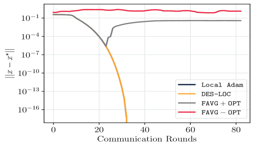
(a)

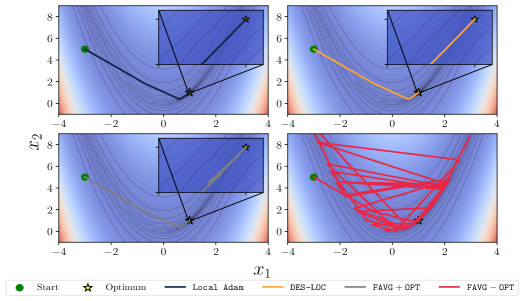
(b)

Figure 2: We present a toy problem where DES-LOC ($K_{x}=192,K_{u}=192,K_{v}=692$) and Local Adam ($K=K_{x}$) both converge to the optimum (overlapping in Fig.˜2(a)). Methods keeping optimizer states local  (Douillard et al., 2023; Sani et al., 2025) fail, causing oscillations without convergence. Periodically resetting states  (Sani et al., 2024; Iacob et al., 2025) similarly stalls due to repeated oscillations. We optimize the non-convex function $f(x_{1},x_{2})=(1-x_{1})^{2}+100(x_{2}-x_{1}^{2})^{2}$ with $M=256$ workers and IID Gaussian noise ($\sigma=1.5$).

3 Convergence Guarantees for DES-LOC

In this section, we provide theoretical support for the proposed DES-LOC approach and demonstrate that synchronizing optimizer states is less critical to overall convergence than model averaging. To keep the presentation concise, we focus on a version of the Adam optimizer that uses only a single momentum state (i.e., SGD with momentum). Extensions to the full Adam optimizer with both momentum states can be carried out using analysis techniques from li2022distributed for convergence in expectation, and from LocalAdam for high-probability guarantees; we provide an informal result here and defer all detailed proofs and technical discussions to the appendix.

Formally, we consider the following optimization problem:

$$\textstyle\min_{x\in\mathbb{R}^{d}}f(x):=\frac{1}{M}\sum_{m=1}^{M}f_{m}(x),\quad\text{with}\quad f_{m}(x)=\mathbb{E}_{\xi\sim\mathcal{D}_{m}}[F_{m}(x;\xi)].$$ (7)

In this setup, all $M$ machines collaboratively minimize the objective in (7). Generally, we assume each machine $m$ has access to only dataset $\mathcal{D}_{m}$, which can differ from device to device. This recovers the homogeneous distribution case when all machines have the same dataset $\mathcal{D}_{1}=\mathcal{D}_{2}=\dots=\mathcal{D}_{M}$ and minimize the same loss $f_{1}(x)=f_{2}(x)=\dots=f_{m}(x)=f(x)$. As in practice, we assume each machine $m$ computes mini-batch stochastic gradients corresponding to randomly selected samples $\xi\sim\mathcal{D}_{m}$ from dataset $\mathcal{D}_{m}$. To derive convergence bounds, we further assume the following standard technical assumptions on the problem structure and stochastic gradients.

Assumption 1 (Lower bound and smoothness).

The overall loss function $f\colon\mathbb{R}^{d}\to\mathbb{R}$ is lower bounded by some $f^{*}\in\mathbb{R}$ and all local loss functions $f_{m}$ are $L$-smooth:

$$\|\nabla f_{m}(x)-\nabla f_{m}(y)\|\leq L\|x-y\|,\quad\text{for any }x,y\in\mathbb{R}^{d}.$$

Assumption 2 (Unbiased noise with bounded stochastic variance).

The stochastic gradient $g^{m}$ of local loss function $f_{m}$ computed by machine $m$ is unbiased and the noise has bounded variance:

$$\mathbb{E}[g^{m}]=\nabla f_{m}(x),\quad\mathbb{E}[\|g_{t}^{m}-\nabla f_{m}(x)\|^{2}]\leq\sigma^{2},\quad\text{for any }x\in\mathbb{R}^{d}.$$

Assumption 3 (Bounded heterogeneity).

For any $x\in\mathbb{R}^{d}$, the heterogeneity is bounded by

$$\textstyle\frac{1}{M}\sum_{m=1}^{M}\|\nabla f_{m}(x)\|^{2}\leq G^{2}+B^{2}\|\nabla f(x)\|^{2}.$$

All three assumptions are standard and widely used in the convergence analysis of optimization algorithms Yu2019; pmlr-v119-karimireddy20a; wang2021fieldguidefederatedoptimization; Yuan2022. Note that the bounded heterogeneity condition recovers the homogeneous case when $G^{2}=0$ and $B^{2}=1$. To facilitate the technical presentation of the analysis, we view model and optimizer state synchronizations through assigning probabilities to each averaging event. Particularly, instead of averaging model parameters every $K_{x}$ steps (i.e., ${\color[rgb]{0,0,1}t\bmod K_{x}=0}$), we average with probability $p_{x}=\frac{1}{K_{x}}$, which are statistically equivalent. In the following theorem, we provide convergence rate of SGDM optimizer under such probabilistic and decoupled synchronization:

Theorem 1.

Let Assumptions 1, 2 and 3 hold. Then, choosing the step size $\eta=\min(\eta_{0},\frac{1}{\sqrt{T}})$ with

$$\textstyle\eta_{0}\stackrel{{\scriptstyle\mathrm{def}}}{{=}}\frac{1}{4L}\min\left(1-\beta,\frac{1}{6\sqrt{\psi\max(1,B^{2}-1)}}\right),\quad\text{where}\quad\psi\stackrel{{\scriptstyle\mathrm{def}}}{{=}}\frac{4(1-p_{x})}{p_{x}^{2}}\cdot\frac{(1-\beta)(1-p_{u})}{1-(1-p_{u})\beta},$$ (8)

the average iterates $x_{t}=\mathbb{E}_{m}[x_{t}^{m}]$ of DES-LOC-SGDM converge with the following rate:

$$\textstyle\frac{1}{T}\sum_{t=0}^{T-1}\mathbb{E}{\|\nabla f(x_{t})\|^{2}}\leq\frac{4}{\sqrt{T}}\left(f(x_{0})-f^{*}+\frac{L\sigma^{2}}{2M}\right)+\mathcal{O}\left(\frac{1+\psi}{T}\right).$$ (9)

We now discuss the convergence result and its implications. First, the obtained rate (9) is asymptotically optimal for this setup (arjevani2023lowerbound). Notably, the leading term $\mathcal{O}(\frac{1}{\sqrt{T}})$ is unaffected by the number of local steps or by the decoupled synchronization approach we propose. Interestingly, probabilities $p_{x}$, $p_{u}$, and the momentum parameter $\beta$ appear only in the higher-order term $\mathcal{O}(\frac{1}{T})$, and thus have a limited impact on the convergence speed. In particular, setting $p_{x}=1$ and $p_{u}=0$ (which implies $\psi=0$) recovers standard mini-batch SGDM and its corresponding convergence rate Liu2020.

Regarding the relative importance of model and optimizer state synchronization steps, it is evident from (8) that model synchronization has a greater impact on convergence due to the dependence $\psi=\mathcal{O}(\frac{1}{p_{x}^{2}})$. Moreover, momentum averaging can be turned off entirely ($p_{u}=0$) without affecting the asymptotic behavior of the rate. Clearly, the same is not true for model averaging: with vanishing $p_{x}$, the $\psi$ term becomes unbounded and breaks the rate. However, since the $\psi$ term also appears in the step-size restriction (8), increasing the frequency $p_{u}$ of momentum averaging—while not changing the asymptotic rate—allows for a larger step size in theory, potentially leading to faster convergence in practice. Overall, the obtained theory justifies the hypothesis that momentum states can be synchronized less frequently than the model parameters and that more averaging improves convergence through supporting larger step sizes.

For DES-LOC-Adam, we generalize the convergence result of (LocalAdam) as follows,

Theorem 2 (Informal).

Let $K_{\mathrm{lcm}}=\mathrm{lcm}\{K_{x},K_{u},K_{\upsilon}\}$, $f$ be weakly-convex and the same assumptions as in Theorem 3 of (LocalAdam), then with probability $\geq 1-\delta$, DES-LOC yields,

$$\frac{1}{K_{\mathrm{lcm}}R}\sum^{R-1}_{r=0}\sum^{K_{\mathrm{lcm}}-1}_{k=0}\|\nabla f(\bar{z}_{r,k})\|^{2}=\tilde{\mathcal{O}}\left(\sqrt{\frac{L\Delta\sigma^{2}}{MK_{\mathrm{lcm}}R}}\right),$$ (10)

where $\bar{z}_{r,k}$ is an auxiliary sequence of $x_{r,k}$, and $\sigma$ bounds stochastic noise (see Appendix for details).

Theorem 2 generalizes the convergence result of local Adam LocalAdam to the case of different state-specific intervals $K_{x},K_{u},K_{\upsilon}$. A full version of Theorem 2 is provided in the Appendix.

4 Experimental Design

Our experimental setup addresses the following research questions:

• Do theoretical rates of change predict the empirical evolution of optimizer states?

• How does the synchronization frequency of a model/optimizer state impact performance?

• To what extent can DES-LOC cut communication w.r.t. Local Adam in practical scenarios?

• How does DES-LOC scale with increasing model size and longer training horizons?

4.1 Experimental Setup

Models and data. Unless noted, we train a $135$M-parameter GPT-style model (see Table˜2) with sequence length $2048$. Following Photon, we distinguish worker batch size $\mathcal{B}_{w}$ from global batch size $\mathcal{B}=\sum_{w=0}^{M-1}\mathcal{B}_{w}$. By default, we evenly split a global batch of $2$M tokens across $M=4$ workers, sampling IID from SmolLM2 (SmolLM2): $70\%$ Fineweb-Edu (FineWeb), $10\%$ Cosmopedia (Cosmopedia), $10\%$ Python-Edu, $5\%$ FineMath 4+, and $5\%$ Infi-WebMath 4+. The $135$M model trains for $6.4$B tokens ($2.4\times$ compute-optimal (TrainingComputeOptimalLLMs)). For RQ4, we scale to $1.7$B for $40$B tokens ($2\times$ compute-optimal) following recent practice (llama3; BeyondChinchilla; SmolLM2). In heterogeneous experiments, each worker samples one dataset component except the Fineweb-Edu worker, which samples the SmolLM2 mixture.

Optimizers. We use Adam (Adam) and its problem-independent variant ADOPT (ADOPT). By modifying the second-moment update, ADOPT guarantees optimal-rate convergence for any $\beta_{2}$ and stabilizes small per-worker batches without altering Adam’s core properties. For the $135$M-parameter experiments, we grid-search $(\beta_{1},\beta_{2},\eta)$ under DDP; the $1.7$B model adopts hyperparameters from SmolLM2; ADOPT. Learning rates follow the warmup-stable-decay (WSD) schedule (BeyondFixedTrainingDuration; SmolLM2). We favor ADOPT with default $\beta_{2}=0.9999$ in high-$\beta$ regimes where Adam is often unstable.

Baselines. We compare DES-LOC with: (i) fully synchronous Adam/ADOPT via DDP; (ii) Local Adam/ADOPT; (iii) FedAvg/Local SGD persistently keeping optimizer states (Photon; DiLoCo), which we call FAVG$+$OPT; and (iv) FedAvg resetting optimizer states (LLMFL; DEPT), which we call FAVG$-$OPT;. Persistent-state FedAvg corresponds to DES-LOC with infinite state sync periods ($K_{u},K_{v}=\infty$), providing an upper bound on communication efficiency. We expect DDP to serve as an upper bound on performance for the machine-learning objective. When discussing hardware robustness, we are concerned with environments prone to systems failures and the repeated re-allocation of workers.

Metrics. We evaluate DES-LOC and baselines by (i) perplexity and (ii) per-worker asymptotic communication cost assuming a bandwidth-optimal Ring-AllReduce (Horovod) algorithm scaling linearly with model size. For the $1.7$B model, we report standard in-context-learning (ICL) benchmarks (gpt3) as they become discriminative at larger scales, we use a zero-shot setting for ICL tasks unless stated otherwise following SmolLM2 and report the best performing communication-efficient method in blue with the best-performing overall in bold. To fairly compare optimizer-state changes across decay rates, we measure their relative rates of change as $\|s_{t+K}-s_{t}\|_{2}/\|s_{t}\|_{2}$. For convergence plot comparisons, we report metric means and standard deviations computed over the last round (shown next to labels). In addition, we provide in the supplementary materials an analysis on the wall-clock time benefits of our approach compared to the baseline, along with our system modeling.

5 Evaluation

Our results show optimizer states change at different rates (Section˜5.1), forming a clear synchronization hierarchy (Section˜5.2). DES-LOC reduces communication $2\times$ vs. Local Adam (Section˜5.3) while converging robustly with adding workers and scaling effectively to large models (Section˜5.4).

5.1 Higher $\beta$ Optimizer States Have Slower Empirical Rates of Change (RQ1)

Figure˜3 shows that relative rates of change for the two momenta in Local ADOPT/Adam scale with their decay rates under gradient clipping ($\rho=1$). Supported by our theoretical discussion on momenta half-lives (Section˜2), the second momentum evolves substantially slower than the first at high-$\beta_{2}$. For Local Adam, the second momentum remains slower even when $\beta_{2}\approx\beta_{1}$, potentially because gradient variance (Adam) evolves slower than the mean direction (first momentum).

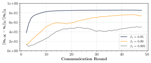
(a)

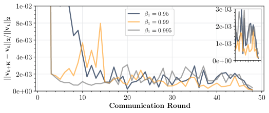
(b)

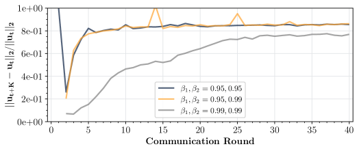
(c)

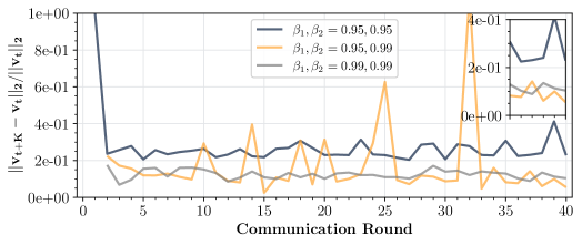
(d)

Figure 3: Relative rates of change for first and second momenta across rounds using standard Local ADOPT/Adam ($K=64$). For ADOPT ($\beta_{2}=0.9999$), increasing $\beta_{1}\geq 0.99$ greatly slows the first-momentum rate of change. The second momentum evolves $\sim 100\times$ slower (note y-axis is in log scale), consistent with their decay rates and half-lives. For Adam, higher $\beta_{1},\beta_{2}$ slow both momenta.

5.2 Parameters Require Frequent Sync, Momenta Sync Proportional to $\beta$ (RQ2)

Figure˜4 evaluates the effect of independently varying synchronization periods ($K_{x},K_{u},K_{v}$) for parameters and optimizer states. We consider two baseline periods ($K_{b}=16,256$), chosen based on the fastest state’s half-life ($\tau_{0.5}(0.95)\approx 13.5$). Frequent parameter synchronization ($K_{x}$) is crucial for performance, while synchronizing momenta ($K_{u},K_{v}$) significantly impacts training only if their half-lives align with the base frequency $K_{b}$. Otherwise, synchronization frequency primarily influences communication costs rather than model quality. Adam results can be seen in Appendix˜C.

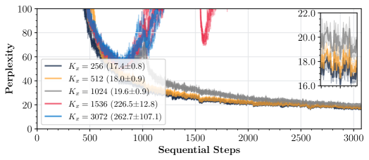
(a)

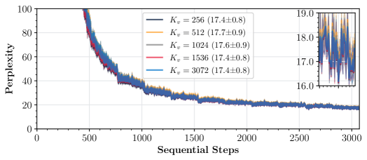
(b)

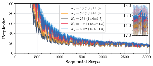
(c)

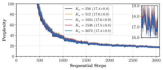
(d)

Figure 4: Model perplexity for DES-LOC (ADOPT, $\beta_{1}=0.95,\beta_{2}=0.9999$), varying synchronization periods independently (others fixed at $K_{b}$). Parameter synchronization (a) is critical, with sharp degradation at higher periods. Second-momentum synchronization (b) minimally affects performance due to its large half-life ($\tau_{0.5}(\beta_{2})\gg K_{b}$). First-momentum synchronization significantly improves perplexity (c) only when the baseline matches its half-life ($K_{b}=16$), having minimal impact otherwise (d). Parameters and second momentum behave similarly across sync frequencies (Appendix˜C)

5.3 DES-LOC Brings $2\times$ Communication Reductions Relative to Local Adam (RQ3)

Figure˜5 shows DES-LOC achieves a $2\times$ communication reduction over the prior state-of-the-art Local Adam (LocalAdam) without significant perplexity degradation, even when adding workers. Synchronizing parameters at $K_{x}=K$ (matching Local Adam) and momenta at $K_{u}=3K_{x}$, $K_{v}=6K_{x}$ consistently yields minimal degradation, aligning with the slower evolution and lower sensitivity of second-momentum sync frequency (Fig.˜4). Other low communication configurations are in Appendix˜C.

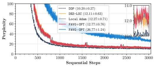
(a)

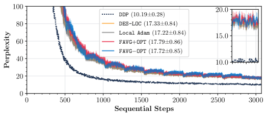
(b)

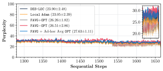
(c)

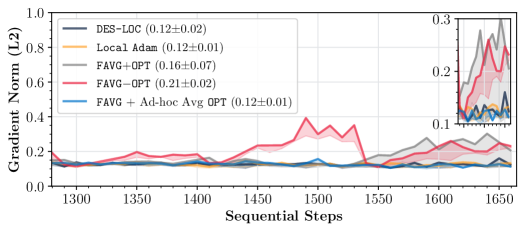
(d)

Figure 5: Setting $K_{x}=K$, $K_{u}=3K_{x}$, and $K_{v}=6K_{x}$, DES-LOC achieves a $\mathbf{2}\times$ communication reduction over Local Adam, matching performance at high (a) and low (b) frequencies for Local Adam and heuristic baselines (see Section˜4.1). We demonstrate robustness to the addition of new workers by doubling worker count at step $1536$ (c,d); DES-LOC and Local Adam remain stable in perplexity/gradient norms, outperforming heuristic methods and ad-hoc optimizer-state averaging.

5.4 DES-LOC Performs Well At Large-scale Long Horizon Training (RQ4)

Figure˜6 shows that DES-LOC reliably scales to billion-scale models and extensive training workloads. Evaluating the billion-scale models on the ICL tasks (Table˜1), DES-LOC remains competitive with all baselines while significantly reducing communication versus Local Adam and DDP. The heuristic baseline (Photon) suffers notable training instabilities (Fig.˜6.b) potentially impacting its downstream performance (Table˜1) and underscoring the advantage of DES-LOC’s training stability.

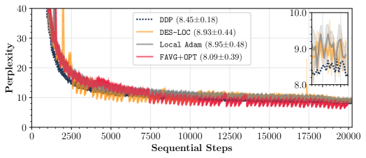
(a)

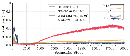
(b)

Figure 6: DES-LOC matches Local Adam perplexity for billion-scale model training at half the communication cost ($K_{x}=256,K_{u}=3K_{x},K_{v}=6K_{x}$), representing a $\mathbf{170}\times$ reduction over DDP. Though initially behind DDP, both DES-LOC and Local Adam quickly converge to competitive perplexity at longer training horizons. Federated Averaging (keeping optimizer states) achieves reasonable performance (a) but suffers activation growth (b) and parameter-norm growth (Appendix˜C), potentially due to noisy local updates, raising concerns for extended training ($\geq 11$ trillion tokens (SmolLM2)).

Table 1: Our billion-scale model trained with DES-LOC matches or surpasses the In-context Learning (ICL) performance of models trained with Local Adam and Federated Averaging (keeping local optimizer states), approaching DDP performance. Federated Averaging (keeping local optimizer states) slightly underperforms compared to its perplexity results from Fig.˜6.a, indicating that the activation increases (Fig.˜6.b) from the unstable training procedure may have damaged the model.

Method	Arc Challenge (arc_challenge)	Arc Easy (arc_challenge)	PIQA (piqa)	HellaSwag (hellaswag)	Avg
DES-LOC	$31.8$	$59.0$	$70.7$	$44.9$	$51.6$
Local Adam	$31.9$	$59.0$	$70.6$	$45.8$	$51.8$
FAVG+OPT	$30.1$	$58.0$	$70.0$	$44.8$	$50.7$
DDP	$\mathbf{33.8}$	$\mathbf{62.5}$	$\mathbf{71.1}$	$\mathbf{47.8}$	$\mathbf{53.8}$

6 Related Work and Limitations

Communication bottlenecks for DDP. In synchronous data-parallel training, workers exchange full gradients or parameters every iteration, incurring linear communication costs using Ring-AllReduce (Horovod). When hardware is weakly connected or widely distributed, communication significantly slows wall-clock training time (Photon) as workers need to wait for synchronization to finish.

Periodic local updates. Federated Averaging (FedAvg) (fedavg) and Local SGD (LocalSGD) reduce communication by performing $K$ local optimization steps before averaging parameters, decreasing communication rounds by a factor of $K$. Although provably convergent for distributed SGD, these guarantees do not extend to adaptive optimizers commonly used for foundation models, due to local optimizer states. Ad-hoc solutions either keep optimizer states local (DiLoCo; DiLoCoScalingLaws; AsyncDiLoCo) or reset them after each sync (LLMFL; Photon), both lacking robust convergence guarantees, unlike Local SGD.

Local stateful optimizers under communication constraints. Adam (Adam) is widely adopted for pre-training because it scales to larger batches than SGD (NoiseIsNotTheMainFactorSGDAdam), suiting large GPU clusters (llama3). It approximates the gradient’s sign (DissectingAdam) using exponential moving averages of gradients and their squares; however, its convergence is not guaranteed as it requires $\beta_{1}<\sqrt{\beta_{2}}<1$, with large, problem-specific $\beta_{2}$ (OnTheConvergenceOfAdamAndBeyond; AdamCanConvergeWithoutAnyModificationToUpdateRules). Other momentum-based and adaptive optimizers (NesterovIlya; LION; LAMB; ADOPT) also track gradient moments. Local Adam (LocalAdam) reduces communication by allowing multiple local optimization steps before global averaging and converges faster than DDP per communication round, provided each worker syncs parameters and optimizer states. However, synchronizing these states triples communication relative to Local SGD/DDP, offsetting the reduced frequency. In general, sync costs scale linearly with the number of optimizer states.

Limitations. First, while our main non-convex convergence result holds for SGDM, in the case of Adam we discuss the analyses (both in expectation and high-probability results) with additional assumptions such as bounded gradient condition and homogeneous data distribution. Nevertheless, these assumptions are commonly used in the non-convex adaptive optimization. Second, due to compute limitations (two machines with 4$\times$A40s and two with 4$\times$H100s), our hyperparameter search was extensive yet constrained to smaller models. Lastly, while our analysis uses Adam/AMSGrad, many experiments use modified Adam (ADOPT) (ADOPT).

7 Conclusion

DES-LOC reconciles communication efficiency with rigorous convergence guarantees in distributed adaptive optimization. By extending theory to the independent synchronization of Adam and SGDM optimizer states, we empirically demonstrate convergence alongside $\mathbf{170\times}$ and $\mathbf{2\times}$ communication reductions over DDP and prior state-of-the-art methods at billion-scale LLM training, even in environments prone to system failures. Our findings yield clear guidelines: i) frequently synchronize parameters, and ii) synchronize optimizer states less often, proportional to their half-lives. These insights open avenues for future research, including layer-wise synchronization, adaptive frequencies, compressed updates, as well as emerging applications, such as worldwide cross-data center training and collaborative training. As training workloads scale, we envision DES-LOC becoming the standard for efficient, resilient foundation-model training in data centers and general distributed environments.

Acknowledgments

All costs for the computational resources used for this work were funded by Flower Labs, and the research conducted by a team of researchers from Flower Labs, The University of Cambridge, The Institute of Science and Technology of Austria, The University of Warwick, and Mohamed bin Zayed University of Artificial Intelligence. Support for university-based researchers came from a variety of sources, but in particular, the following funding organizations are acknowledged: the European Research Council (REDIAL), the Royal Academy of Engineering (DANTE), the Ministry of Education of Romania through the Credit and Scholarship Agency, and the European Union’s Horizon 2020 research and innovation programme under the Marie Skłodowska-Curie grant agreement No 101034413.

parttocA Table of Contents

Appendix

Appendix B Experimental Details and Optimizer Hyperparameter Sweeps (See Section˜4.1)

Here we provide additional experimental details complementing those in Section˜4.1, including: a) model architecture details and hyperparameters independent of optimizer choice (Section˜B.1), b) our hyperparameter sweep procedure to select optimizer-specific settings (Section˜B.2), and c) the optimal hyperparameters with those used in Section˜5 highlighted in bold.

B.1 Architecture Details and Hyperparameters

Table 2: Model architecture and training parameters. We denote the number of transformer blocks by #Blocks, number of attention heads by #Heads, embedding dimension by $d_{\mathrm{model}}$, vocabulary size by $|\mathcal{V}|$, and feedforward-layer expansion by Exp. Ratio. All models use positional embeddings (RopeEmbeddings), the silu activation function, and norm-based gradient clipping with clip-bound $\rho$. Global batch size (summed across all workers) is $|\mathcal{B}_{\mathrm{G}}|$, and sequence length is standard for models at these scales. For model initialization we use $\sigma=\nicefrac{{1}}{{\sqrt{d_{\mathrm{model}}}}}$. The total number of steps is denoted by $T$.

Model Size	Blocks	$\bm{d_{\mathrm{model}}}$	$\mathbf{|\mathcal{V}|}$	#Heads	Exp. Ratio	ROPE $\theta$	ACT	Init $\sigma$	$\rho$	Seq Len	$\mathbf{|\mathcal{B}_{\mathrm{G}}|}$	$\mathbf{T}$
$135$M	$30$	$576$	$50$K	$9$	$4$	$10000$	silu	$0.04$	$1.0$	$2048$	$1024$	$1536,3072$
$1.7$B	$24$	$2048$	$50$K	$16$	$4$	$10000$	silu	$0.02$	$1.0$	$2048$	$1024$	$20480$

Table˜2 summarizes the architectural details of our models, following established practices for large language models at their respective scales. Unless otherwise stated, we adopt the hyperparameters recommended by SmolLM2 for both the $135$M and the $1.7$B models. We operate at a batch size of $2$M tokens, which is very large for the $135$M model at the length of training we perform (HowDoesBatchSizeScaleInPreTraining) and industry-standard for the $1.7$B model (llama2), we chose to operate at large batch sizes because adaptive optimizers provide benefits primarily in large-batch training regimes (NoiseIsNotTheMainFactorSGDAdam). Moreover, we intend DES-LOC for use in cross data-center scenarios, where effectively utilizing available accelerators naturally demands large batch sizes and/or model scales. For both model sizes, we train for approximately $2\times$ the compute-optimal token budget (TrainingComputeOptimalLLMs), placing our evaluations within the context of extended-duration foundation model training (SmolLM2). Our chosen token budget is conservative due to resource constraints; for comparison, SmolLM2 used $11$ trillion tokens which is over $4000\times$ compute-optimal for the $135$M model, and $300\times$ for the $1.7$B.

We select warmup and decay schedules following recommendations from HowDoesBatchSizeScaleInPreTraining; BeyondFixedTrainingDuration; SmolLM2. For the $135$M model, the warmup period is set to $T_{\mathrm{WARM}}=512$ steps, corresponding to the roughly $40\%$ of the compute-optimal training tokens recommended by HowDoesBatchSizeScaleInPreTraining. For the $1.7$B model, we use the recommended $T_{\mathrm{WARM}}=2048$ steps from SmolLM2, roughly $10\%$ of total training. The stable-decay period uses a $1-\mathrm{SQRT}$ schedule over the final $T_{\mathrm{DECAY}}=10\%\times T$ steps (BeyondFixedTrainingDuration). For shorter runs, such as $T=1536$ during heterogeneous-data evaluations, we keep the warmup fixed and proportionally scale the decay to ensure well-conditioned parameter updates during the stable learning rate period. The seeds we use for data sampling and for controlling the training algorithms and model are provided in the code accompanying the appendix.

B.2 Optimizer Parameters Sweeping Procedure

As detailed in Section˜2 and verified empirically in Section˜5.2, the choice of decay rates $\beta_{1},\beta_{2}$ strongly influences the effective synchronization frequencies achievable by both DES-LOC and Local Adam. This relationship arises directly from the half-life of optimizer states, given by $\tau_{0.5}=\frac{\ln(0.5)}{\ln(\beta)}$.

For Adam, prior studies such as StableLowPrecisionTrainingLLMLVM have demonstrated a critical interplay between the learning rate ($\eta$), batch size, and the second-momentum decay $\beta_{2}$. Specifically, increasing either the learning rate or batch size typically demands a lower $\beta_{2}$ to maintain training stability and avoid loss spikes. Conversely, higher $\beta_{2}$ values constrain the learning rate and batch size. Such dynamics have also been recently observed between the learning rate and the first-momentum decay $\beta_{1}$ in AdemaMix. Given that all our experiments use a fixed large batch size of roughly $2$ million tokens (appropriate for billion-scale training), we systematically tune the learning rate $\eta$ in response to changes in $\beta_{1},\beta_{2}$. We try values of $\beta_{1},\beta_{2}$ based on previous works (HowDoesBatchSizeScaleInPreTraining) and follow the theoretical convergence requirement of AdamCanConvergeWithoutAnyModificationToUpdateRules setting $\beta_{1}\leq\sqrt{\beta_{2}}$.

Due to computational constraints, we cannot jointly optimize synchronization periods, data distributions, and decay parameters, and instead adopt a structured two-stage tuning approach:

1. Stage 1: Tuning $\eta$ for DDP. Starting from the recommended baseline learning rate ($\eta_{0}$) from SmolLM2, we conduct a grid search as outlined by DiLoCoScalingLaws: $\{\dots,\sqrt{2}^{-2}\eta_{0},\sqrt{2}^{-1}\eta_{0},\eta_{0},\sqrt{2}\eta_{0},\sqrt{2}^{2}\eta_{0},\dots\}$ We expand this search until perplexity stops improving, identifying an optimal learning rate $\eta^{\ast}_{\texttt{DDP}}$ for each $(\beta_{1},\beta_{2})$ configuration.

2. Stage 2: Tuning $\eta$ for Local Adam. We then repeat this procedure for Local Adam, using $\eta^{\ast}_{\texttt{DDP}}$ as the new baseline. To balance generalizability and computational cost, we set the synchronization period to an intermediate value of $K=64$, between high-frequency ($K=16$) and low-frequency ($K=256$) scenarios.

Additionally, following HowDoesBatchSizeScaleInPreTraining, we omit weight decay (set to zero) to simplify the hyperparameter tuning process, as it directly affects only model parameters, not optimizer states.

B.2.1 Optimizers’ Hyperparameter Configurations

Table 3: Optimal learning rates $\eta^{\ast}$ for $\beta_{1},\beta_{2}$ configurations of ADOPT/Adam. The hyperparameter sweep procedure (see Section˜B.2) involves incrementally adjusting the learning rate by factors of $\sqrt{2}$ around the initial value from SmolLM2 until performance stops improving.

Optimizer	$\mathbf{\beta_{1}}$	$\mathbf{\beta_{2}}$	$\eta^{\ast}$
ADOPT	$0.9$	$0.9999$	$0.0021$
	$\mathbf{0.95}$	$\mathbf{0.9999}$	$\mathbf{0.0021}$
	$0.99$	$0.9999$	$0.0014$
	$0.995$	$0.9999$	$0.0007$
Adam	$0.9$	$0.95$	$0.0042$
	$\mathbf{0.95}$	$\mathbf{0.95}$	$\mathbf{0.003}$
	$0.9$	$0.99$	$0.003$
	$0.95$	$0.99$	$0.003$
	$0.99$	$0.99$	$0.0021$

Our hyperparameter sweep (Table˜3) indicates that the optimal learning rate $\eta^{\ast}$ under the warmup-stable-decay scheduler (BeyondFixedTrainingDuration) strongly depends on both optimizer type and the chosen $\beta_{1},\beta_{2}$ values. For Adam, optimal learning rates and second-momentum decay ($\beta_{2}$) align closely with recommendations from SmolLM2, though a slightly higher first-momentum decay ($\beta_{1}$) consistently performs better, in agreement with prior findings (HowDoesBatchSizeScaleInPreTraining). For ADOPT (default $\beta_{2}$), we observe a lower optimal learning rate compared to Adam, but similar best-performing $\beta_{1}$ values. We also find that the optimal learning rate does not differ between DDP and Local Adam for given $\beta_{1},\beta_{2}$ when $K=64$ and using a $\sqrt{2}$ sweep, higher learning rates either do not provide a benefit or diverge while lower learning rates are only necessary when pushing $K$ far closer to the complete training duration.

We find that increasing $\beta_{1}$ for ADOPT, and $\beta_{1},\beta_{2}$ for Adam, leads to rapid performance degradation, particularly at or above $0.99$. Since the half-life at $\beta=0.99$ ($\tau_{0.5}\approx 69$) is not sufficiently longer than at $\beta=0.95$ ($\tau_{0.5}\approx 13.5$) to justify the observed performance drop, we select $\beta_{1}=0.95$ for all experiments, along with the default $\beta_{2}$ for ADOPT and $\beta_{2}=0.95$ for Adam.

Appendix C Complementary Results to Sections˜2.1 and 5

We now provide additional results supplementing those presented in the main text. Specifically:

1. Section˜C.1 complements Fig.˜2(a) by including results on the heterogeneous data distribution described in Section˜4.1. This highlights DES-LOC’s robustness under imperfect sampling or strongly Non-IID federated scenarios (see AdancesAndOpenProblems, Sec 3.1).

2. Section˜C.2.1 complements Fig.˜4 by showing the separate impact of varying synchronization frequencies for parameters and the second momentum when the base frequency is $K_{b}=16$. It supports our claim that parameters and second momentum exhibit similar behavior across different synchronization regimes, unlike the first momentum.

3. Section˜C.2.2 extends Fig.˜4 by evaluating DES-LOC-Adam. We confirm that the parameter synchronization frequency is the most important, as predicted by our theory. In contrast, the momenta sync frequency is far less impactful, especially for low parameter sync frequencies.

4. Section˜C.3.1 complements Fig.˜5 by showing DES-LOC-ADOPT’s perplexity against baseline methods on heterogeneous data (as defined in Section˜4.1). This validates our claim from Contribution 2 regarding DES-LOC’s effectiveness on heterogeneous datasets.

5. Section˜C.3.2 presents an ablation study examining alternative low-communication configurations of DES-LOC, justifying our choice of $K_{u}=3K_{x},K_{v}=6K_{x}$ used in Fig.˜5.

6. Section˜C.3.3 repeats the baseline comparison from Fig.˜5 for DES-LOC-Adam, demonstrating that DES-LOC achieves similar communication reductions and performance when using Adam instead of ADOPT.

7. Section˜C.4 provides additional metrics illustrating training instabilities for the FAVG+OPT baseline, including rapidly growing parameter norms, supporting observations in Fig.˜6.b.

C.1 Toy Problem on Non-IID Data (See Fig.˜2(a))

(a)

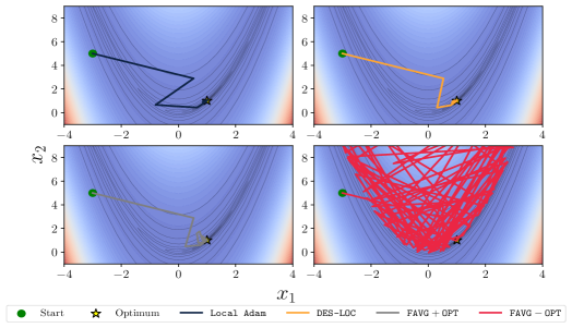
(b)

Figure 7: We present a toy problem in a Non-IID setting, where DES-LOC (with synchronization periods $K_{x}=192,K_{u}=192,K_{v}=692$) and Local Adam (with $K=K_{x}$) converge to a superior solution compared to methods that keep optimizer states local  (DiLoCo; Photon) or periodically reset them  (LLMFL; DEPT). Like the IID scenario, resetting optimizer states prevents convergence due to repeated oscillations caused by reinitializations. Additionally, as seen in panel (a) between rounds $15$ and $40$, methods keeping optimizer states local suffer from larger oscillations further away from the optimum. The function optimized is $f(x_{1},x_{2})=(1-x_{1})^{2}+100(x_{2}-x_{1}^{2})^{2}$, and we simulate $M=256$ workers, each adding Gaussian noise with worker-specific standard deviation $\sigma^{m}\sim\mathcal{N}(0,3)$.

C.2 RQ2: Independent Sync Frequencies

This section provides supplementary results for RQ2, complementing Section˜5.2. Section˜C.2.1 shows that perplexity has similar sensitivity to the first and second momentum synchronization frequencies at both high and low base synchronization frequencies. Additionally, Section˜C.2.2 repeats the comparison from Fig.˜4 for DES-LOC-Adam, revealing similar trends regarding the importance of the parameters, with a reduced importance for the momenta due to lower $\beta_{2}$.

C.2.1 Parameter and Second Momentum At $K_{b}=16$ (See Fig.˜4.a,Fig.˜4.b)

Figure˜8 examines the effects of independently varying synchronization periods ($K_{x},K_{v}$) for parameters and second momentum under DES-LOC-ADOPT in the high-frequency regime ($K_{b}=16$), chosen based on the first momentum’s half-life ($\tau_{0.5}\approx 13.5$). Similar to the low-frequency results in Fig.˜4.a, parameter synchronization frequency ($K_{x}$) strongly influences perplexity, while the second momentum ($K_{v}$) has minimal impact due to its long half-life. This contrasts with the first momentum, whose half-life closely matches the high-frequency period.

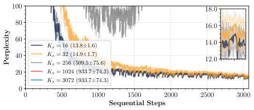
(a)

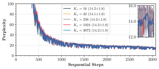
(b)

Figure 8: Model perplexity for DES-LOC (ADOPT, $\beta_{1}=0.95,\beta_{2}=0.9999$), independently varying synchronization periods at a high baseline frequency ($K_{b}=16$). Similar to Fig.˜4, parameter synchronization (a) is critical, with performance sharply degrading at higher periods, while second-momentum synchronization (b) has minimal impact due to its large half-life ($\tau_{0.5}(\beta_{2})\gg K_{b}$).

C.2.2 Adam Results (See Fig.˜4)

Figure˜9 provides complementary results to Figs.˜4 and 8 using DES-LOC-Adam with $\beta_{1}=\beta_{2}=0.95$. Unlike ADOPT, the relatively low $\beta$ result in both the first and second momentum quickly adapting to the local gradients, reducing the impact of their sync frequency.

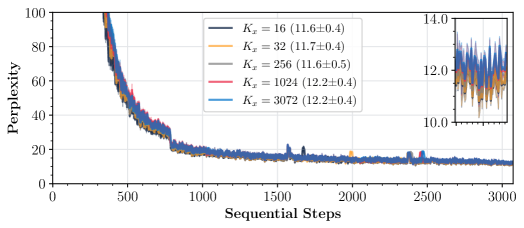
(a)

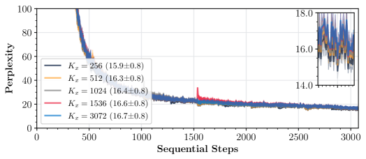
(b)

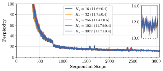
(c)

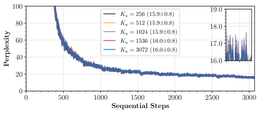
(d)

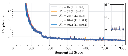
(e)

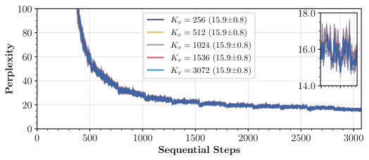
(f)

Figure 9: Model perplexity for DES-LOC-Adam ($\beta_{1}=\beta_{2}=0.95$) when independently varying sync periods ($K_{x},K_{u},K_{v}$) while fixing others at baseline $K_{b}$. Parameter synchronization (a,b) influences performance in both high ($K_{b}=16$) and low ($K_{b}=256$) frequency regimes. Momenta synchronization minimally impacts perplexity due to both states’ high adaptivity (low $\beta$), with potentially minor effects during the early stages of training in high-frequency regimes (c,e).

C.3 RQ3: Communication Reduction And Baseline Comparisons

This section provides supplementary results for RQ3, complementing Section˜5.3. Section˜C.3.1 shows the perplexity of different configurations providing a $2\times$ communication reduction over Local Adam. Additionally, Section˜C.3.3 repeats the comparison against baselines from Section˜5.3 for DES-LOC-Adam, showing similar communication reductions relative to Local Adam.

C.3.1 DES-LOC on Heterogeneous Data (See Contribution 2)

Figure˜10 evaluates the robustness of DES-LOC against baselines under heterogeneous (Non-IID) data distributions as described in Section˜4.1. We set synchronization periods to $K_{x}=K$, $K_{u}=3K_{x}$, and $K_{v}=6K_{x}$ to achieve a targeted $\mathbf{2}\times$ communication reduction over Local Adam.

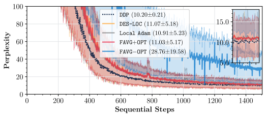
(a)

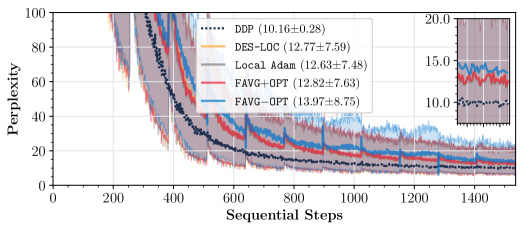
(b)

Figure 10: Comparison of perplexity under Non-IID conditions for DES-LOC, Local Adam ($K_{x}=K_{u}=K_{v}$), and heuristic baselines (defined in Section˜4.1) at high (a) and low (b) synchronization frequencies. Due to higher cross-worker variance caused by heterogeneous data, parameters require slightly more frequent synchronization in the low-frequency regime ($K_{x}=128<256$). Experiments are limited to $T=1536$ steps ($\sim$compute-optimal) for computational feasibility.

C.3.2 DES-LOC Low Communication Configurations Ablation (See Fig.˜5)

Figure˜11 explores alternative synchronization configurations enabling DES-LOC to achieve improved communication efficiency over Local Adam. Motivated by theoretical insights (Sections˜2 and 3) and empirical evidence (Sections˜5.1 and 5.2), we only consider settings where parameter synchronization is most frequent ($K_{x}\leq\min(K_{u},K_{v})$). This constraint follows from experiments in Section˜5.2, which show that infrequent parameter synchronization significantly degrades perplexity, while momentum synchronization frequency has a smaller impact. For a fixed $2\times$ communication reduction over Local Adam, our findings confirm that synchronizing the first momentum more frequently than the second aligns with their respective half-lives and maintains performance close to Local Adam.

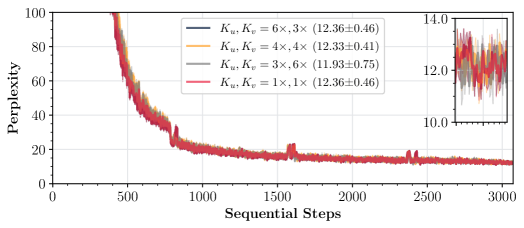
(a)

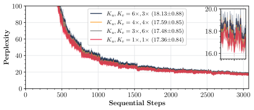
(b)

Figure 11: Configurations of DES-LOC targeting $2\times$ lower communication than Local Adam ($K_{x}=K_{u}=K_{v}$), setting $K_{u},K_{v}$ as multiples of $K_{x}$. In both high (a) and low-frequency (b) regimes, performance depends on how communication is split between momenta for $\beta_{1}\ll\beta_{2}$. Syncing the first momentum less often ($K_{u}=6K_{x},K_{v}=3K_{x}$) degrades performance, wasting communication on the slow second momentum. Conversely, syncing it frequently ($K_{u}=3K_{x},K_{v}=6K_{x}$) yields performance comparable to Local Adam. Setting $K_{u}=K_{v}=4K_{x}$ produces intermediate results.

C.3.3 Adam Results (See Fig.˜5)

We now present results for DES-LOC-Adam with $\beta_{1}=\beta_{2}=0.95$. DES-LOC-Adam achieves similar communication reductions over Local Adam and DDP as ADOPT. However, due to the lower $\beta_{2}$, the second-momentum half-life ($\tau_{0.5}(0.95)\approx 13.5$) is significantly shorter than for ADOPT ($\tau_{0.5}(0.9999)\approx 6931$). Figure˜12 shows that with both momenta evolving at similar rates, the benefit of selecting $K_{u}<K_{v}$ diminishes. For consistency and due to meaningful empirical differences in rates of change (Section˜5.1), we keep $K_{u}=3\times K_{x}$ and $K_{v}=6\times K_{x}$ in subsequent comparisons.

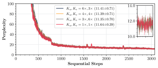
(a)

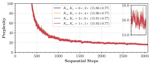
(b)

Figure 12: Configurations of DES-LOC targeting $2\times$ lower communication than Local Adam ($K_{x}=K_{u}=K_{v}$), using Adam ($\beta_{1}=\beta_{2}=0.95$). In contrast to DES-LOC-ADOPT (where $\beta_{1}\ll\beta_{2}$ yields an advantage for $K_{u}<K_{v}$ as shown in Fig.˜11), the similar half-lives in Adam make perplexity insensitive to how communication is split between momenta for high (a) and low-frequencies (b).

Figure˜13 shows DES-LOC-Adam achieves a $2\times$ communication reduction over the prior state-of-the-art Local Adam (LocalAdam) without significant perplexity degradation. Due to the much faster evolution of the optimizer states using Adam compared to ADOPT, local worker gradients drive the optimization reducing the benefit of allocating more of the communication budget to the first momentum.

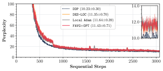
(a)

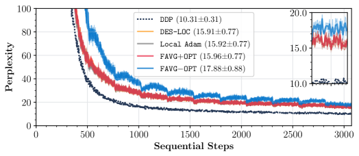
(b)

Figure 13: Setting $K_{x}=K$, $K_{u}=3K_{x}$, and $K_{v}=6K_{x}$, DES-LOC-Adam achieves a $\mathbf{2}\times$ communication reduction over Local Adam, matching performance at high (a) and low (b) frequencies for Local Adam and heuristic baselines (see Section˜4.1).

C.4 RQ4: Additional Metrics and Training Instabilities of FAVG$+$OPT (See Fig.˜6.b)

Figure˜14 complements Fig.˜6.b by showing parameter and update norms for DES-LOC and baseline methods when training billion-scale models. Both DES-LOC and Local Adam regularize updates by synchronizing optimizer states, effectively reducing update norms due to averaging across workers (triangle inequality). In contrast, the heuristic baseline (Photon) experiences large updates, leading to uncontrolled parameter growth, increased activations (Fig.˜6.b), and degraded performance on downstream ICL tasks (Table˜1) relative to its perplexity (Fig.˜6.a).

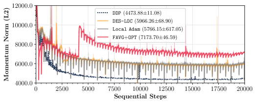
(a)

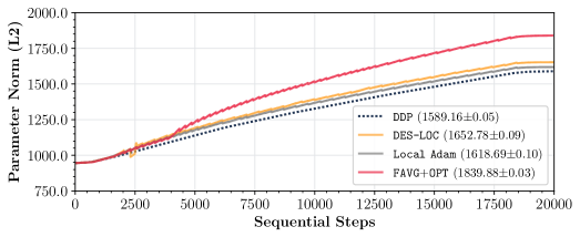
(b)

Figure 14: Comparison of update (a) and parameter norms (b) for billion-scale models trained with DES-LOC ($K_{x}=256,K_{u}=768,K_{v}=1536$), Local Adam ($K=256$), DDP, and Federated Averaging with persistent optimizer states (FAVG$+$OPT). Frequent synchronization in Local Adam and DDP consistently reduces update and parameter norms. Similarly, DES-LOC achieves comparable reductions at intervals corresponding to multiples of $\mathtt{lcm}(K_{x},K_{u},K_{v})$, with smaller intermediate drops. Conversely, FAVG$+$OPT, which does not synchronize optimizer states, experiences persistently larger and noisier updates, becoming vulnerable to spikes (notably before step $5000$). This leads to uncontrolled parameter growth (b).

Appendix D Deterministic Optimizer-specific Variants of Algorithm˜1

Algorithm 2 DES-LOC-Adam

1:Model tensors, Hyper-parameters

2: $x_{0}$,$u_{-1},v_{-1}\in\mathbb{R}^{d}$ — initial parameter vector,seeds for first and second moments

3: $\{\eta_{t}\}_{t=0}^{T-1}\subset\mathbb{R}_{>0}$ — step-size schedule

4: $\beta_{1},\beta_{2}\in[0,1)$ — Adam decay factors

5: $\rho,\lambda\in\mathbb{R}_{>0}$ — gradient clipping term, $\ell_{2}$ stability term

6: $T,M\in\mathbb{N}_{+}$ — total iterations, number of workers

7: $K_{x},K_{u},K_{v}$ $\in\mathbb{N}_{+}$ — sync periods for parameters, first and second moments

8:$x_{T},\;u_{T-1},v_{T-1}$

9:for each worker $m$: $x_{0}^{m}=x_{0},\;u_{-1}^{m}=v_{-1}^{m}=0$ local init ($t=-1$ seeds)

10:for $t=0,\dots,T-1$ do training loop

11:  for all workers $m=0,\dots,M-1$ in parallel do

12:    $g_{t}^{m}\leftarrow\nabla F(x_{t}^{m};\xi_{t}^{m})$ stochastic gradient

13:    $\widehat{g}_{t}^{m}\leftarrow\textbf{clip}(g_{t}^{m},\rho)$ clip to radius $\rho$

14:    if $t\bmod K_{u}=0$ then sync $u$

15:     $u_{t}^{m}\leftarrow\beta_{1}\,\mathbb{E}_{m}[u_{t-1}^{m}]+(1-\beta_{1})\widehat{g}_{t}^{m}$

16:    else

17:     $u_{t}^{m}\leftarrow\beta_{1}\,u_{t-1}^{m}+(1-\beta_{1})\widehat{g}_{t}^{m}$     

18:    if $t\bmod K_{v}=0$ then sync $v$

19:     $v_{t}^{m}\leftarrow\beta_{2}\,\mathbb{E}_{m}[v_{t-1}^{m}]+(1-\beta_{2})(\widehat{g}_{t}^{m}\odot\widehat{g}_{t}^{m})$

20:    else

21:     $v_{t}^{m}\leftarrow\beta_{2}\,v_{t-1}^{m}+(1-\beta_{2})(\widehat{g}_{t}^{m}\odot\widehat{g}_{t}^{m})$     

22:    $d_{t}^{m}\leftarrow\dfrac{\eta_{t}}{\sqrt{v_{t}^{m}+\lambda^{2}}}\odot u_{t}^{m}$ bias-corrected step

23:    if $t\bmod K_{x}=0$ then sync $x$

24:     $x_{t+1}^{m}\leftarrow\mathbb{E}_{m}[x_{t}^{m}]-d_{t}^{m}$

25:    else

26:     $x_{t+1}^{m}\leftarrow x_{t}^{m}-d_{t}^{m}$       

Algorithm 3 DES-LOC-ADOPT

1:Model tensors,Hyper-parameters

2: $x_{0},m_{-1},v_{-1}\in\mathbb{R}^{d}$ — initial parameter vector and momenta

3: $\{\eta_{t}\}_{t=0}^{T-1}\subset\mathbb{R}_{>0}$ — learning rate schedule

4: $\beta_{1},\beta_{2}\in[0,1)$ — decay factors

5: $\rho,\epsilon\in\mathbb{R}_{>0}$ — gradient clipping term,small stability constant

6: $T,M\in\mathbb{N}_{+}$ — total iterations,number of workers

7: $K_{x},K_{m},K_{v}$ $\in\mathbb{N}_{+}$ — sync periods for parameters, first and second moments

8:$x_{T},\;m_{T-1},v_{T-1}$

9:for each worker $m$: $x_{0}^{m}=x_{0},\;m_{-1}^{m}=v_{-1}^{m}=0$ local initialization

10:for $t=0,\dots,T-1$ do

11:  for all workers $m=0,\dots,M-1$ in parallel do

12:    $g_{t}^{m}\leftarrow\nabla F(x_{t}^{m};\xi_{t}^{m})$ stochastic gradient

13:    $\widehat{g}_{t}^{m}\leftarrow\textbf{clip}(g_{t}^{m},\rho)$ gradient clipping

14:    if $t\bmod K_{v}=0$ then

15:     $v_{t}^{m}\leftarrow\beta_{2}\,\mathbb{E}_{m}[v_{t-1}^{m}]+(1-\beta_{2})(\widehat{g}_{t}^{m}\odot\widehat{g}_{t}^{m})$

16:    else

17:     $v_{t}^{m}\leftarrow\beta_{2}\,v_{t-1}^{m}+(1-\beta_{2})(\widehat{g}_{t}^{m}\odot\widehat{g}_{t}^{m})$     

18:    if $t\bmod K_{m}=0$ then

19:     $m_{t}^{m}\leftarrow\beta_{1}\,\mathbb{E}_{m}[m_{t-1}^{m}]+(1-\beta_{1})\frac{\widehat{g}_{t}^{m}}{\max\{\sqrt{v_{t-1}^{m}},\epsilon\}}$

20:    else

21:     $m_{t}^{m}\leftarrow\beta_{1}\,m_{t-1}^{m}+(1-\beta_{1})\frac{\widehat{g}_{t}^{m}}{\max\{\sqrt{v_{t-1}^{m}},\epsilon\}}$     

22:    $d_{t}^{m}\leftarrow\eta_{t}m_{t}^{m}$ ADOPT update

23:    if $t\bmod K_{x}=0$ then

24:     $x_{t+1}^{m}\leftarrow\mathbb{E}_{m}[x_{t}^{m}]-d_{t}^{m}$

25:    else

26:     $x_{t+1}^{m}\leftarrow x_{t}^{m}-d_{t}^{m}$       

Appendix E Convergence Analysis of DES-LOC-SGDM (in expectation bounds)

Here we provide a non-convex convergence analysis of the proposed DES-LOC approach applied to the SGDM optimizer which has a single state ($N=1$, momentum). The complete description of the algorithm can be found in Algorithm 4.

Algorithm 4 DES-LOC-SGDM

1:Model tensors

2: $x_{0}\in\mathbb{R}^{d}$ — initial parameter vector

3: $u_{-1}\in\mathbb{R}^{d}$ — seed for the momentum, initialised to 0

4:Hyper-parameters

5: $\{\eta_{t}\}_{t=0}^{T-1}\subset\mathbb{R}_{>0}$ — step-size schedule

6: $\beta\in[0,1)$ — Momentum decay factor

7: $T\in\mathbb{N}_{+}$ — total optimisation iterations

8: $M\in\mathbb{N}_{+}$ — number of workers

9: $p_{x}=\frac{1}{K_{x}},p_{u}=\frac{1}{K_{u}}$ $\in[0,1]$ — synchronization probabilities for parameters and momentum

10:$x_{T},\;u_{T-1},v_{T-1}$

11:for each worker $m$: $x_{0}^{m}=x_{0},\;u_{-1}^{m}=v_{-1}^{m}=0$ local init ($t=-1$ seeds)

12:for $t=0,\dots,T-1$ do training loop

13:  for all workers $m=0,\dots,M-1$ in parallel do

14:    $g_{t}^{m}\leftarrow\nabla F_{m}(x_{t}^{m};\xi_{t}^{m})$ stochastic gradient

15:    $u_{t}^{m}\leftarrow\begin{cases}\mathbb{E}_{m}[\beta u_{t-1}^{m}+(1-\beta)g_{t}^{m}],&{\color[rgb]{0,0,1}\text{with probability }p_{u}}\\ \beta u_{t-1}^{m}+(1-\beta)g_{t}^{m},&\text{with probability }1-p_{u}\end{cases}$ sync $u$

16:    $x_{t+1}^{m}\leftarrow\begin{cases}\mathbb{E}_{m}[x_{t}^{m}-\eta_{t}u_{t}^{m}],&{\color[rgb]{0,0,1}\text{with probability }p_{x}}\\ x_{t}^{m}-\eta_{t}u_{t}^{m},&\text{with probability }1-p_{x}\end{cases}$ sync $x$   

In order to facilitate the technical presentation, we model synchronization frequencies by assigning probabilities to each averaging event. For example, the parameters $x_{t}^{m}$ are synchronized with the probability $p_{x}=\frac{1}{K_{x}}$, which is statistically equivalent to performing the averaging in every $\frac{1}{p_{x}}=K_{x}$ iteration. Similarly, momentum $u_{t}^{m}$ synchronization happens with probability $p_{u}=\frac{1}{K_{u}}$, which can differ from $p_{x}$.

Step 1 (virtual iterates). For each step $t\geq 0$, denote the average parameters, momentum and gradient as follows:

$$x_{t}\stackrel{{\scriptstyle\mathrm{def}}}{{=}}\mathbb{E}_{m}[x_{t}^{m}],\quad u_{t}\stackrel{{\scriptstyle\mathrm{def}}}{{=}}\mathbb{E}_{m}[u_{t}^{m}],\quad g_{t}\stackrel{{\scriptstyle\mathrm{def}}}{{=}}\mathbb{E}_{m}[g_{t}^{m}].$$

Then these averaged variables follow the “standard” centralized SGDM dynamics:

$$u_{t} = \beta u_{t-1}+(1-\beta)g_{t}$$

$$x_{t+1} = x_{t}-\eta u_{t}.$$

Letting $x_{-1}=x_{0}$, define the global virtual iterations as follows

$$z_{t}\stackrel{{\scriptstyle\mathrm{def}}}{{=}}\frac{1}{1-\beta}x_{t}-\frac{\beta}{1-\beta}x_{t-1},\quad t\geq 0.$$

The key property of this virtual iterates we are going to exploit in the next steps is that they follow averaged gradients, namely for any $t\geq 0$ we have

$$z_{t+1}-z_{t} = \frac{1}{1-\beta}(x_{t+1}-x_{t})-\frac{\beta}{1-\beta}(x_{t}-x_{t-1})$$

$$= -\frac{\eta}{1-\beta}u_{t}+\frac{\eta\beta}{1-\beta}u_{t-1}=-\frac{\eta}{1-\beta}(u_{t}-\beta u_{t-1})=-\eta g_{t}.$$

Step 2 (smoothness over virtual iterates). Then we apply smoothness of the global loss function $f$ over these global virtual iterates.

$$f(z_{t+1}) \leq f(z_{t})+\langle\nabla f(z_{t}),z_{t+1}-z_{t}\rangle+\frac{L}{2}\|z_{t+1}-z_{t}\|^{2}$$

$$= f(z_{t})+\underbrace{\langle\nabla f(x_{t}),z_{t+1}-z_{t}\rangle}_{I}+\underbrace{\langle\nabla f(z_{t})-\nabla f(x_{t}),z_{t+1}-z_{t}\rangle}_{II}+\underbrace{\frac{L}{2}\|z_{t+1}-z_{t}\|^{2}}_{III}.$$

In the next step, we separately bound each term appearing in the above bound.

Step 3a (one step progress). Bounding term I.

$$\mathbb{E}{\langle\nabla f(x_{t}),z_{t+1}-z_{t}\rangle}$$

$$= -\eta\mathbb{E}{\left\langle\nabla f(x_{t}),\frac{1}{M}\sum_{m=1}^{M}g_{t}^{m}\right\rangle}=-\eta\mathbb{E}{\left\langle\nabla f(x_{t}),\frac{1}{M}\sum_{m=1}^{M}\nabla f_{m}(x_{t}^{m})\right\rangle}$$

$$= -\frac{\eta}{2}\mathbb{E}{\|\nabla f(x_{t})\|^{2}}-\frac{\eta}{2}\mathbb{E}{\left\|\frac{1}{M}\sum_{m=1}^{M}\nabla f_{m}(x_{t}^{m})\right\|^{2}}+\frac{\eta}{2}\mathbb{E}{\left\|\nabla f(x_{t})-\frac{1}{M}\sum_{m=1}^{M}\nabla f_{m}(x_{t}^{m})\right\|^{2}}$$

$$= -\frac{\eta}{2}\mathbb{E}{\|\nabla f(x_{t})\|^{2}}-\frac{\eta}{2}\mathbb{E}{\left\|\frac{1}{M}\sum_{m=1}^{M}\nabla f_{m}(x_{t}^{m})\right\|^{2}}+\frac{\eta}{2}\mathbb{E}{\left\|\frac{1}{M}\sum_{m=1}^{M}\nabla f_{m}(x_{t})-\nabla f_{m}(x_{t}^{m})\right\|^{2}}$$

$$\leq -\frac{\eta}{2}\mathbb{E}{\|\nabla f(x_{t})\|^{2}}-\frac{\eta}{2}\mathbb{E}{\left\|\frac{1}{M}\sum_{m=1}^{M}\nabla f_{m}(x_{t}^{m})\right\|^{2}}+\frac{\eta}{2M}\sum_{m=1}^{M}\mathbb{E}{\left\|\nabla f_{m}(x_{t})-\nabla f_{m}(x_{t}^{m})\right\|^{2}}$$

$$\leq -\frac{\eta}{2}\mathbb{E}{\|\nabla f(x_{t})\|^{2}}-\frac{\eta}{2}\mathbb{E}{\left\|\frac{1}{M}\sum_{m=1}^{M}\nabla f_{m}(x_{t}^{m})\right\|^{2}}+\frac{\eta L^{2}}{2M}\sum_{m=1}^{M}\underbrace{\mathbb{E}{\left\|x_{t}-x_{t}^{m}\right\|^{2}}}_{\rm Lemma\;\ref{lem:x-xm}}.$$

Step 3b (one step progress). Bounding term II.

$$\mathbb{E}{\langle\nabla f(z_{t})-\nabla f(x_{t}),z_{t+1}-z_{t}\rangle} = -\eta\mathbb{E}{\left\langle\nabla f(z_{t})-\nabla f(x_{t}),\frac{1}{M}\sum_{m=1}^{M}\nabla f_{m}(x_{t}^{m})\right\rangle}$$

$$\leq \frac{\eta\rho}{2}\mathbb{E}{\|\nabla f(z_{t})-\nabla f(x_{t})\|^{2}}+\frac{\eta}{2\rho}\mathbb{E}{\left\|\frac{1}{M}\sum_{m=1}^{M}\nabla f_{m}(x_{t}^{m})\right\|^{2}}$$

$$\leq \frac{\eta\rho L^{2}}{2}\underbrace{\mathbb{E}{\|z_{t}-x_{t}\|^{2}}}_{\rm Lemma\;\ref{lem:z-x}}+\frac{\eta}{2\rho}\mathbb{E}{\left\|\frac{1}{M}\sum_{m=1}^{M}\nabla f_{m}(x_{t}^{m})\right\|^{2}}.$$

Step 3c (one step progress). Bounding term III.

$$\frac{L}{2}\mathbb{E}{\|z_{t+1}-z_{t}\|^{2}} = \frac{\eta^{2}L}{2}\mathbb{E}{\left\|\frac{1}{M}\sum_{m=1}^{M}g_{t}^{m}\right\|^{2}}$$

$$= \frac{\eta^{2}L}{2}\mathbb{E}{\left\|\frac{1}{M}\sum_{m=1}^{M}g_{t}^{m}-\nabla f_{m}(x_{t}^{m})\right\|^{2}}+\frac{\eta^{2}L}{2}\mathbb{E}{\left\|\frac{1}{M}\sum_{m=1}^{M}\nabla f_{m}(x_{t}^{m})\right\|^{2}}$$

$$= \frac{\eta^{2}L}{2M^{2}}\sum_{m=1}^{M}\mathbb{E}{\left\|g_{t}^{m}-\nabla f_{m}(x_{t}^{m})\right\|^{2}}+\frac{\eta^{2}L}{2}\mathbb{E}{\left\|\frac{1}{M}\sum_{m=1}^{M}\nabla f_{m}(x_{t}^{m})\right\|^{2}}$$

$$\leq \frac{\eta^{2}L}{2M}\sigma^{2}+\frac{\eta^{2}L}{2}\mathbb{E}{\left\|\frac{1}{M}\sum_{m=1}^{M}\nabla f_{m}(x_{t}^{m})\right\|^{2}}.$$

Step 3abc (one step progress). Combining previous bounds.

$$\mathbb{E}{f(z_{t+1})}-\mathbb{E}{f(z_{t})} \leq \mathbb{E}\underbrace{\langle\nabla f(x_{t}),z_{t+1}-z_{t}\rangle}_{I}+\mathbb{E}\underbrace{\langle\nabla f(z_{t})-\nabla f(x_{t}),z_{t+1}-z_{t}\rangle}_{II}+\mathbb{E}\underbrace{\frac{L}{2}\|z_{t+1}-z_{t}\|^{2}}_{III}$$

$$\leq -\frac{\eta}{2}\mathbb{E}{\|\nabla f(x_{t})\|^{2}}-\frac{\eta}{2}\mathbb{E}{\left\|\frac{1}{M}\sum_{m=1}^{M}\nabla f_{m}(x_{t}^{m})\right\|^{2}}+\frac{\eta L^{2}}{2M}\sum_{m=1}^{M}\underbrace{\mathbb{E}{\left\|x_{t}-x_{t}^{m}\right\|^{2}}}_{\rm Lemma\;\ref{lem:x-xm}}$$

$$+\;\frac{\eta\rho L^{2}}{2}\underbrace{\mathbb{E}{\|z_{t}-x_{t}\|^{2}}}_{\rm Lemma\;\ref{lem:z-x}}+\frac{\eta}{2\rho}\mathbb{E}{\left\|\frac{1}{M}\sum_{m=1}^{M}\nabla f_{m}(x_{t}^{m})\right\|^{2}}$$

$$+\;\frac{\eta^{2}L}{2K}\sigma^{2}+\frac{\eta^{2}L}{2}\mathbb{E}{\left\|\frac{1}{M}\sum_{m=1}^{M}\nabla f_{m}(x_{t}^{m})\right\|^{2}}$$

$$\leq -\frac{\eta}{2}\mathbb{E}{\|\nabla f(x_{t})\|^{2}}-\frac{\eta}{2}\left(1-\frac{1}{\rho}-\eta L\right)\mathbb{E}{\left\|\frac{1}{M}\sum_{m=1}^{M}\nabla f_{m}(x_{t}^{m})\right\|^{2}}$$

$$+\;\frac{\eta\rho L^{2}}{2}\underbrace{\mathbb{E}{\|z_{t}-x_{t}\|^{2}}}_{\rm Lemma\;\ref{lem:z-x}}+\frac{\eta L^{2}}{2M}\sum_{m=1}^{M}\underbrace{\mathbb{E}{\left\|x_{t}-x_{t}^{m}\right\|^{2}}}_{\rm Lemma\;\ref{lem:x-xm}}+\frac{\eta^{2}L}{2M}\sigma^{2}.$$

Step 4 (final). Now we average over the iterates and apply the bounds derived in Lemmas 1,2.

$$\frac{\mathbb{E}[f(z_{T})-f(z_{0})]}{T} = \frac{1}{T}\sum_{t=0}^{T-1}\mathbb{E}[f(z_{t+1})-f(z_{t})]$$

$$\leq -\frac{\eta}{2T}\sum_{t=0}^{T-1}\mathbb{E}{\|\nabla f(x_{t})\|^{2}}-\frac{\eta}{2}\left(1-\frac{1}{\rho}-\eta L\right)\frac{1}{T}\sum_{t=0}^{T-1}\mathbb{E}{\left\|\frac{1}{M}\sum_{m=1}^{M}\nabla f_{m}(x_{t}^{m})\right\|^{2}}$$

$$+\;\frac{\eta\rho L^{2}}{2}\underbrace{\frac{1}{T}\sum_{t=0}^{T-1}\mathbb{E}{\|z_{t}-x_{t}\|^{2}}}_{\rm Lemma\;1}+\frac{\eta L^{2}}{2}\underbrace{\frac{1}{TM}\sum_{t=0}^{T-1}\sum_{m=1}^{M}\mathbb{E}{\left\|x_{t}-x_{t}^{m}\right\|^{2}}}_{\rm Lemma\;2}+\frac{\eta^{2}L}{2M}\sigma^{2}$$

$$\leq -\frac{\eta}{2T}\sum_{t=0}^{T-1}\mathbb{E}{\|\nabla f(x_{t})\|^{2}}-\frac{\eta}{2}\left(1-\frac{1}{\rho}-\eta L\right)\frac{1}{T}\sum_{t=0}^{T-1}\mathbb{E}{\left\|\frac{1}{M}\sum_{m=1}^{M}\nabla f_{m}(x_{t}^{m})\right\|^{2}}+\frac{\eta^{2}L}{2M}\sigma^{2}$$

$$+\;\frac{\eta\rho L^{2}}{2}\left(\frac{\eta^{2}\beta^{2}}{(1-\beta)^{2}M}\sigma^{2}+\frac{\eta^{2}\beta^{2}}{(1-\beta)^{2}}\frac{1}{T}\sum_{\tau=0}^{T-1}\mathbb{E}\left\|\frac{1}{M}\sum_{m=1}^{M}\nabla f_{m}(x_{\tau}^{m})\right\|^{2}\right)$$

$$+\;\frac{\eta L^{2}}{2}\left(12\eta^{2}(B^{2}-1)\psi\cdot\frac{1}{T}\sum_{t=0}^{T-1}\mathbb{E}\|\nabla f(\theta^{t})\|^{2}+4\eta^{2}\psi(\sigma^{2}+3G^{2})\right)$$

$$\leq -\frac{\eta}{2}\left(1-12\eta^{2}L^{2}(B^{2}-1)\psi\right)\frac{1}{T}\sum_{t=0}^{T-1}\mathbb{E}{\|\nabla f(x_{t})\|^{2}}$$

$$-\;\frac{\eta}{2}\left(1-\frac{1}{\rho}-\eta L-\frac{\eta^{2}\beta^{2}\rho L^{2}}{(1-\beta)^{2}}\right)\frac{1}{T}\sum_{t=0}^{T-1}\mathbb{E}{\left\|\frac{1}{M}\sum_{m=1}^{M}\nabla f_{m}(x_{t}^{m})\right\|^{2}}$$

$$+\;\frac{\eta^{2}L}{2M}\sigma^{2}+\frac{\eta^{3}\rho L^{2}\beta^{2}}{2(1-\beta)^{2}M}\sigma^{2}+2\eta^{3}L^{2}\psi(\sigma^{2}+3G^{2}).$$

Next, we choose $\rho=2$ and step size $\eta$ such that

$$12\eta^{2}L^{2}(B^{2}-1)\psi\leq\frac{1}{2} \iff$$ to bound the first term

$$\eta L+\frac{2\eta^{2}\beta^{2}L^{2}}{(1-\beta)^{2}}\leq\frac{1}{2} \iff$$ to bound the second term

$$12\eta^{2}L^{2}\psi\leq\frac{1}{2} \iff$$ from Lemma 4

Note that

$$\eta_{0}\stackrel{{\scriptstyle\mathrm{def}}}{{=}}\frac{1}{4L}\min\left(1-\beta,\frac{1}{6\sqrt{\psi\max(1,B^{2}-1)}}\right)$$

satisfies all three bounds. Then, with any $\eta\leq\eta_{0}$ we get

$$\frac{\mathbb{E}[f(z_{T})-f(z_{0})]}{T} \leq -\frac{\eta}{4T}\sum_{t=0}^{T-1}\mathbb{E}{\|\nabla f(x_{t})\|^{2}}$$

$$+\;\frac{\eta^{2}L}{2M}\sigma^{2}+\frac{\eta^{3}\rho L^{2}\beta^{2}}{2(1-\beta)^{2}M}\sigma^{2}+2\eta^{3}L^{2}\psi(\sigma^{2}+3G^{2}).$$

Noticing that $z_{0}=x_{0}$ and $f^{*}\leq f(z_{T})$, we have

$$\frac{1}{T}\sum_{t=0}^{T-1}\mathbb{E}{\|\nabla f(x_{t})\|^{2}}\leq\frac{4(f(x_{0})-f^{*})}{\eta T}+\frac{2\eta L}{M}\sigma^{2}+\frac{4\eta^{2}L^{2}\beta^{2}}{(1-\beta)^{2}M}\sigma^{2}+8\eta^{2}L^{2}\psi(\sigma^{2}+3G^{2}).$$

Furthermore, choosing $\eta=\min(\eta_{0},\frac{1}{\sqrt{T}})$, we get the following rate:

$$\frac{1}{T}\sum_{t=0}^{T-1}\mathbb{E}{\|\nabla f(x_{t})\|^{2}}$$

$$\leq \max\left(1,\frac{1}{\eta_{0}\sqrt{T}}\right)\frac{4(f(x_{0})-f^{*})}{\sqrt{T}}+\frac{2L\sigma^{2}}{M\sqrt{T}}+\frac{4L^{2}\beta^{2}\sigma^{2}}{(1-\beta)^{2}MT}+\frac{8L^{2}\psi(\sigma^{2}+3G^{2})}{T}$$

$$\leq \frac{4(f(x_{0})-f^{*})}{\sqrt{T}}+\frac{2L\sigma^{2}}{M\sqrt{T}}+\frac{4(f(x_{0})-f^{*})}{\eta_{0}T}+\frac{4L^{2}\beta^{2}\sigma^{2}}{(1-\beta)^{2}MT}+\frac{8L^{2}\psi(\sigma^{2}+3G^{2})}{T}$$

$$= \frac{4}{\sqrt{T}}\left(f(x_{0})-f^{*}+\frac{L\sigma^{2}}{2M}\right)+\mathcal{O}\left(\frac{1+\psi}{T}\right).$$

E.1 Extension to Adam optimizer

Here we discuss extension of the previous analysis for the Adam optimizer including the second-order momentum in the analysis. The addition is similar to the first-order momentum while the synchronization probability $p_{v}$ can differ from other probabilities $p_{u}$ and $p_{u}$. The complete description of the algorithm can be found in Algorithm 5. Instead of bounded heterogeneity Assumption 3, in this analysis we use stronger condition mentioned below:

Assumption 4 (Bounded gradient).

For any iterate $t\geq 0$ and worker $m$, the local stochastic gradient is bounded, namely $\|g_{t}^{m}\|_{2}\leq G$.

This condition facilitates the analysis by providing uniform upper bounds for gradients/momentum variables and is commonly used in the analysis of adaptive optimization.

Algorithm 5 DES-LOC-Adam (with probabilistic synchronization)

1:Model tensors

2: $x_{0}\in\mathbb{R}^{d}$ — initial parameter vector

3: $u_{-1},v_{-1}\in\mathbb{R}^{d}$ — seeds for first and second moments, initialised to 0

4:Hyper-parameters

5: $\{\eta_{t}\}_{t=0}^{T-1}\subset\mathbb{R}_{>0}$ — step-size schedule

6: $\beta_{1},\beta_{2}\in[0,1)$ — Adam decay factors

7: $\lambda\in\mathbb{R}_{\geq 0}$ — $\ell_{2}$ stability term

8: $T\in\mathbb{N}_{+}$ — total optimisation iterations

9: $M\in\mathbb{N}_{+}$ — number of workers

10: $p_{x}=\frac{1}{K_{x}},p_{u}=\frac{1}{K_{u}},p_{v}=\frac{1}{K_{v}}$ $\in[0,1]$ — synchronization probabilities for parameters and momentums

11:$x_{T},\;u_{T-1},v_{T-1}$

12:for each worker $m$: $x_{0}^{m}=x_{0},\;u_{-1}^{m}=v_{-1}^{m}=0$ local init ($t=-1$ seeds)

13:for $t=0,\dots,T-1$ do training loop

14:  for all workers $m=0,\dots,M-1$ in parallel do

15:    $g_{t}^{m}\leftarrow\nabla F(x_{t}^{m};\xi_{t}^{m})$ stochastic gradient

16:    $u_{t}^{m}\leftarrow\begin{cases}\mathbb{E}_{m}[\beta_{1}u_{t-1}^{m}+(1-\beta_{1})g_{t}^{m}],&{\color[rgb]{0,0,1}\text{with probability }p_{u}}\\ \beta_{1}u_{t-1}^{m}+(1-\beta_{1})g_{t}^{m},&\text{with probability }1-p_{u}\end{cases}$ sync $u$

17:    $v_{t}^{m}\leftarrow\begin{cases}\mathbb{E}_{m}[\beta_{2}v_{t-1}^{m}+(1-\beta_{2})(g_{t}^{m}\odot g_{t}^{m})],&{\color[rgb]{0,0,1}\text{with probability }p_{v}}\\ \beta_{2}v_{t-1}^{m}+(1-\beta_{2})(g_{t}^{m}\odot g_{t}^{m}),&\text{with probability }1-p_{v}\end{cases}$ sync $u$

18:    $\tilde{v}_{t}^{m}\leftarrow\max(v_{t}^{m},\tilde{v}_{t-1}^{m})$ AMSGrad Normalization, $\tilde{v}_{-1}=v_{-1}$

19:    $d_{t}^{m}\leftarrow\dfrac{\eta_{t}}{\sqrt{\tilde{v}_{t}^{m}+\lambda^{2}}}\odot u_{t}^{m}$ bias-corrected update

20:    $x_{t+1}^{m}\leftarrow\begin{cases}\mathbb{E}_{m}[x_{t}^{m}-d_{t}^{m}],&{\color[rgb]{0,0,1}\text{with probability }p_{x}}\\ x_{t}^{m}-d_{t}^{m},&\text{with probability }1-p_{x}\end{cases}$ sync $x$   

Step 1 (preconditioning and virtual iterates). Let $\Gamma_{t}^{m}\stackrel{{\scriptstyle\mathrm{def}}}{{=}}\mbox{\bf diag}^{-\nicefrac{{1}}{{2}}}(\tilde{v}_{t}^{m}+\lambda^{2})$ be the preconditioning matrix and for each step $t\geq 0$, denote the averaged variables

$$x_{t}\stackrel{{\scriptstyle\mathrm{def}}}{{=}}\mathbb{E}_{m}[x_{t}^{m}],\quad u_{t}\stackrel{{\scriptstyle\mathrm{def}}}{{=}}\mathbb{E}_{m}[u_{t}^{m}],\quad v_{t}\stackrel{{\scriptstyle\mathrm{def}}}{{=}}\mathbb{E}_{m}[v_{t}^{m}],\quad\tilde{v}_{t}\stackrel{{\scriptstyle\mathrm{def}}}{{=}}\mathbb{E}_{m}[\tilde{v}_{t}^{m}],\quad g_{t}\stackrel{{\scriptstyle\mathrm{def}}}{{=}}\mathbb{E}_{m}[g_{t}^{m}].$$

Then

$$u_{t} = \beta_{1}u_{t-1}+(1-\beta_{1})g_{t}$$

$$x_{t+1} = x_{t}-d_{t}=x_{t}-\eta\mathbb{E}_{m}[\Gamma_{t}^{m}u_{t}^{m}].$$

Consider the same averaged iterates $x_{t}$ and virtual iterates $z_{t}$ as before:

$$z_{t}=\frac{1}{1-\beta_{1}}x_{t}-\frac{\beta_{1}}{1-\beta_{1}}x_{t-1}.$$

In particular, $z_{0}=x_{0}$. Then,

$$z_{t+1}-z_{t} = \frac{1}{1-\beta_{1}}(x_{t+1}-x_{t})-\frac{\beta_{1}}{1-\beta_{1}}(x_{t}-x_{t-1})$$

$$= -\frac{\eta}{1-\beta_{1}}\mathbb{E}_{m}[\Gamma_{t}^{m}u_{t}^{m}]+\frac{\eta\beta_{1}}{1-\beta_{1}}\mathbb{E}_{m}[\Gamma_{t-1}^{m}u_{t-1}^{m}]$$

$$= -\frac{\eta}{1-\beta_{1}}\mathbb{E}_{m}[\Gamma_{t}^{m}u_{t}^{m}]+\frac{\eta\beta_{1}}{1-\beta_{1}}\mathbb{E}_{m}[\Gamma_{t-1}^{m}u_{t-1}^{m}]\pm\frac{\eta\beta_{1}}{1-\beta_{1}}\mathbb{E}_{m}[\Gamma_{t}^{m}u_{t-1}^{m}]$$

$$= -\frac{\eta}{1-\beta_{1}}\mathbb{E}_{m}[\Gamma_{t}^{m}(u_{t}^{m}-\beta_{1}u_{t-1}^{m})]+\frac{\eta\beta_{1}}{1-\beta_{1}}\mathbb{E}_{m}[(\Gamma_{t-1}^{m}-\Gamma_{t}^{m})u_{t-1}^{m}]$$

$$= -\eta\mathbb{E}_{m}[\Gamma_{t}^{m}\widetilde{g}_{t}^{m}]+\frac{\eta\beta_{1}}{1-\beta_{1}}\mathbb{E}_{m}[(\Gamma_{t-1}^{m}-\Gamma_{t}^{m})u_{t-1}^{m}]$$

$$= -\eta\mathbb{E}_{m}[\Gamma_{t}^{m}g_{t}]+\eta\mathbb{E}_{m}[\Gamma_{t}^{m}(g_{t}-\widetilde{g}_{t}^{m})]+\frac{\eta\beta_{1}}{1-\beta_{1}}\mathbb{E}_{m}[(\Gamma_{t-1}^{m}-\Gamma_{t}^{m})u_{t-1}^{m}]$$

$$= -\eta\Gamma_{t}g_{t}+\eta\cdot\underbrace{\mathbb{E}_{m}[\Gamma_{t}^{m}(g_{t}-\widetilde{g}_{t}^{m})]}_{\stackrel{{\scriptstyle\mathrm{def}}}{{=}}U_{t}}+\eta\cdot\underbrace{\frac{\beta_{1}}{1-\beta_{1}}\mathbb{E}_{m}[(\Gamma_{t-1}^{m}-\Gamma_{t}^{m})u_{t-1}^{m}]}_{\stackrel{{\scriptstyle\mathrm{def}}}{{=}}V_{t}},$$

where $\Gamma_{t}\stackrel{{\scriptstyle\mathrm{def}}}{{=}}\mathbb{E}_{m}[\Gamma_{t}^{m}]$ and $\widetilde{g}_{t}^{m}\stackrel{{\scriptstyle\mathrm{def}}}{{=}}\frac{u_{t}^{m}-\beta_{1}u_{t-1}^{m}}{1-\beta_{1}}$ for which, $\mathbb{E}_{m}[\widetilde{g}_{t}^{m}]=\mathbb{E}_{m}[g_{t}^{m}]=g_{t}$.

Step 2 (smoothness over virtual iterates). Then we apply smoothness of the global loss function $f$ over these global virtual iterates.

$$f(z_{t+1})-f(z_{t}) \leq \langle\nabla f(z_{t}),z_{t+1}-z_{t}\rangle+\frac{L}{2}\|z_{t+1}-z_{t}\|^{2}$$

$$= -\eta\left\langle\nabla f(z_{t}),\Gamma_{t}g_{t}\right\rangle+\eta\langle\nabla f(z_{t}),U_{t}\rangle+\eta\langle\nabla f(z_{t}),V_{t}\rangle+\frac{L}{2}\|z_{t+1}-z_{t}\|^{2}$$

$$= \underbrace{-\eta\left\langle\nabla f(x_{t}),\Gamma_{t}g_{t}\right\rangle}_{I}+\underbrace{\eta\langle\nabla f(z_{t}),U_{t}\rangle}_{II}+\underbrace{\eta\left\langle\nabla f(z_{t}),V_{t}\right\rangle}_{III}$$

$$+\;\underbrace{\frac{\eta^{2}L}{2}\left\|\Gamma_{t}g_{t}-U_{t}-V_{t}\right\|^{2}}_{IV}+\underbrace{\eta\left\langle\nabla f(x_{t})-\nabla f(z_{t}),\Gamma_{t}g_{t}\right\rangle}_{V}.$$

In the next step, we separately bound each term appearing in the above bound. For clarity, we are also going to use $\|\nabla f(x_{t})\|\leq G$ and $\|\nabla f(z_{t})\|\leq G$. However, these conditions can be avoided through linking $\nabla f(z_{t})$ term to $\nabla f(x_{t})$, and $\nabla f(x_{t})$ term to $\mathbb{E}_{m}\nabla f_{m}(x_{t}^{m})$ with the bound for $\mathbb{E}[\|x_{t}-x_{t}^{m}\|^{2}]$.

Step 3a (one step progress). Bounding term I.

$$I = -\eta\left\langle\nabla f(x_{t}),\Gamma_{t}g_{t}]\right\rangle$$

$$= -\eta\mathbb{E}\left[\left\langle\nabla f(x_{t}),\Gamma_{t-1}g_{t}\right\rangle\right]+\eta\mathbb{E}\left[\left\langle\nabla f(x_{t}),(\Gamma_{t-1}-\Gamma_{t})g_{t}\right\rangle\right]$$

$$\leq -\eta\mathbb{E}\left[\left\langle\nabla f(x_{t}),\frac{1}{M}\sum_{m=1}^{M}\nabla f_{m}(x_{t}^{m})\right\rangle_{\Gamma_{t-1}}\right]+\eta G^{2}\mathbb{E}[\|\Gamma_{t-1}-\Gamma_{t}\|].$$

$$\leq -\frac{\eta}{2}\mathbb{E}\left[\|\nabla f(x_{t})\|^{2}_{\Gamma_{t-1}}\right]-\frac{\eta}{2}\mathbb{E}\left[\left\|\frac{1}{M}\sum_{m=1}^{M}\nabla f_{m}(x_{t}^{m})\right\|^{2}_{\Gamma_{t-1}}\right]$$

$$+\;\frac{\eta}{2}\mathbb{E}\left[\left\|\nabla f(x_{t})-\frac{1}{M}\sum_{m=1}^{M}\nabla f_{m}(x_{t}^{m})\right\|^{2}_{\Gamma_{t-1}}\right]+\eta G^{2}\mathbb{E}[\|\Gamma_{t-1}-\Gamma_{t}\|]$$

$$\leq -\frac{\eta}{2}\|\Gamma_{t-1}\|_{\min}\mathbb{E}\|\nabla f(x_{t})\|^{2}-\frac{\eta}{2}\mathbb{E}\left[\left\|\frac{1}{M}\sum_{m=1}^{M}\nabla f_{m}(x_{t}^{m})\right\|^{2}_{\Gamma_{t-1}}\right]$$

$$+\;\frac{\eta}{2}\|\Gamma_{t-1}\|_{\max}\mathbb{E}\left[\left\|\frac{1}{M}\sum_{m=1}^{M}\nabla f_{m}(x_{t})-\nabla f_{m}(x_{t}^{m})\right\|^{2}\right]+\eta G^{2}\mathbb{E}[\|\Gamma_{t-1}-\Gamma_{t}\|]$$

$$\leq -\frac{\eta}{2C_{0}}\mathbb{E}\|\nabla f(x_{t})\|^{2}-\frac{\eta}{2}\mathbb{E}\left[\left\|\frac{1}{M}\sum_{m=1}^{M}\nabla f_{m}(x_{t}^{m})\right\|^{2}_{\Gamma_{t-1}}\right]$$

$$+\;\frac{\eta}{2\lambda M}\sum_{m=1}^{M}\mathbb{E}\left[\left\|\nabla f_{m}(x_{t})-\nabla f_{m}(x_{t}^{m})\right\|^{2}\right]+\eta G^{2}\mathbb{E}[\|\Gamma_{t-1}-\Gamma_{t}\|]$$

$$\leq -\frac{\eta}{2C_{0}}\mathbb{E}\|\nabla f(x_{t})\|^{2}+\frac{\eta L^{2}}{2\lambda M}\sum_{m=1}^{M}\mathbb{E}\left[\|x_{t}-x_{t}^{m}\|^{2}\right]+\eta G^{2}\mathbb{E}[\|\Gamma_{t-1}-\Gamma_{t}\|],$$

where $\|\cdot\|$ indicates the spectral norm for matrices, and we used the following inequalities:

$$\|\Gamma_{t-1}\|_{\min}=\left\|\frac{1}{M}\sum_{m=1}^{M}\Gamma_{t-1}^{m}\right\|_{\min}=\frac{1}{M}\sum_{m=1}^{M}\Gamma_{t-1}^{m}[i,i]=\frac{1}{M}\sum_{m=1}^{M}\frac{1}{\sqrt{\tilde{v}_{t-1}[i]+\lambda^{2}}}\geq\frac{1}{\sqrt{G^{2}+\lambda^{2}}}\stackrel{{\scriptstyle\mathrm{def}}}{{=}}\frac{1}{C_{0}}.$$

Step 3b (one step progress). Bounding term II.

$$II = \eta\langle\nabla f(z_{t}),U_{t}\rangle\leq\eta\|\nabla f(z_{t})\|\|U_{t}\|\leq\frac{\eta G}{M}\sum_{m=1}^{M}\|\Gamma_{t}^{m}(g_{t}-\widetilde{g}_{t}^{m})\|$$

$$\leq \frac{\eta G}{\lambda M}\sum_{m=1}^{M}\|g_{t}-\widetilde{g}_{t}^{m}\|.$$

Step 3c (one step progress). Bounding term III.

$$III = \eta\langle\nabla f(z_{t}),V_{t}\rangle\leq\eta\|\nabla f(z_{t})\|\|V_{t}\|\leq\frac{\eta\beta_{1}}{1-\beta_{1}}\frac{G}{M}\sum_{m=1}^{M}\|(\Gamma_{t-1}^{m}-\Gamma_{t}^{m})u_{t-1}^{m}\|$$

$$\leq \frac{\eta\beta_{1}}{1-\beta_{1}}\frac{G^{2}}{M}\sum_{m=1}^{M}\|\Gamma_{t-1}^{m}-\Gamma_{t}^{m}\|.$$

Step 3d (one step progress). Bounding term IV.

$$IV = \frac{\eta^{2}L}{2}\left\|\Gamma_{t}g_{t}-U_{t}-V_{t}\right\|^{2}$$

$$\leq \frac{3\eta^{2}L}{2}\left\|\Gamma_{t}g_{t}\right\|^{2}+\frac{3\eta^{2}L}{2}\left\|U_{t}\right\|^{2}+\frac{3\eta^{2}L}{2}\left\|V_{t}\right\|^{2}$$

$$\leq \frac{3\eta^{2}LG^{2}}{2\lambda^{2}}+\frac{3\eta^{2}L}{2\lambda^{2}M}\sum_{m=1}^{M}\left\|g_{t}-\widetilde{g}_{t}^{m}\right\|^{2}+\frac{3\eta^{2}\beta_{1}LG}{2(1-\beta_{1})M}\sum_{m=1}^{M}\left\|\Gamma_{t-1}^{m}-\Gamma_{t}^{m}\right\|^{2}$$

Step 3e (one step progress). Bounding term V.

$$V = \eta\left\langle\nabla f(x_{t})-\nabla f(z_{t}),\Gamma_{t}g_{t}\right\rangle$$

$$= \eta\mathbb{E}\left[\left\langle\nabla f(x_{t})-\nabla f(z_{t}),\Gamma_{t-1}g_{t}\right\rangle\right]+\eta\mathbb{E}\left[\left\langle\nabla f(x_{t})-\nabla f(z_{t}),(\Gamma_{t}-\Gamma_{t-1})g_{t}\right\rangle\right]$$

$$\leq \eta\mathbb{E}\left[\left\langle\nabla f(x_{t})-\nabla f(z_{t}),\frac{1}{M}\sum_{m=1}^{M}\nabla f_{m}(x_{t}^{m})\right\rangle_{\Gamma_{t-1}}\right]+\frac{\eta^{2}L\beta_{1}}{1-\beta_{1}}\mathbb{E}\left[\left\|\mathbb{E}_{m}[\Gamma_{t-1}^{m}u^{m}_{t-1}]\right\|\|(\Gamma_{t}-\Gamma_{t-1})g_{t}\|\right]$$

$$\leq \eta\mathbb{E}\left[\left\langle\nabla f(x_{t})-\nabla f(z_{t}),\nabla f(x_{t})\right\rangle_{\Gamma_{t-1}}\right]$$

$$+\;\eta\mathbb{E}\left[\left\langle\nabla f(x_{t})-\nabla f(z_{t}),\frac{1}{M}\sum_{m=1}^{M}\nabla f_{m}(x_{t}^{m})-\nabla f_{m}(x_{t})\right\rangle_{\Gamma_{t-1}}\right]+\frac{\eta^{2}L\beta_{1}G^{2}}{(1-\beta_{1})\lambda}\mathbb{E}\left[\|\Gamma_{t}-\Gamma_{t-1}\|\right]$$

$$\leq \frac{\eta}{\lambda}\mathbb{E}\left[\|\nabla f(x_{t})-\nabla f(z_{t})\|\|\nabla f(x_{t})\|\right]$$

$$+\;\frac{\eta}{\lambda}\mathbb{E}\left[\|\nabla f(x_{t})-\nabla f(z_{t})\|\cdot\frac{1}{M}\sum_{m=1}^{M}\|\nabla f_{m}(x_{t}^{m})-\nabla f_{m}(x_{t})\|\right]+\frac{\eta^{2}L\beta_{1}G^{2}}{(1-\beta_{1})\lambda}\mathbb{E}\left[\|\Gamma_{t}-\Gamma_{t-1}\|\right]$$

$$\leq \frac{\eta}{\lambda}\mathbb{E}\left[\frac{1}{2\rho}\|\nabla f(x_{t})-\nabla f(z_{t})\|^{2}+\frac{\rho}{2}\|\nabla f(x_{t})\|^{2}\right]$$

$$+\;\frac{\eta}{\lambda}\mathbb{E}\left[\frac{1}{2}\|\nabla f(x_{t})-\nabla f(z_{t})\|^{2}+\frac{1}{2}\frac{L^{2}}{M}\sum_{m=1}^{M}\|x_{t}^{m}-x_{t}\|^{2}\right]+\frac{\eta^{2}L\beta_{1}G^{2}}{(1-\beta_{1})\lambda}\mathbb{E}\left[\|\Gamma_{t}-\Gamma_{t-1}\|\right],$$

where we used the following uniform bound on $\|\nabla f(x_{t})-\nabla f(z_{t})\|$:

$$\left\|\nabla f(x_{t})-\nabla f(z_{t})\right\| \leq L\left\|x_{t}-z_{t}\right\|\leq\frac{\beta_{1}L}{1-\beta_{1}}\left\|x_{t}-x_{t-1}\right\|=\frac{\eta\beta_{1}L}{1-\beta_{1}}\left\|\mathbb{E}_{m}[\Gamma_{t-1}^{m}u_{t-1}^{m}]\right\|$$

$$\leq \frac{\eta\beta_{1}L}{1-\beta_{1}}\mathbb{E}_{m}[\left\|\Gamma_{t-1}^{m}\|\|u_{t-1}^{m}]\right\|\leq\frac{\eta\beta_{1}L}{1-\beta_{1}}\frac{G}{\lambda}.$$

Therefore, ignoring the constants, we have the following bounds:

$$V \leq \mathcal{O}\left(\frac{\eta^{2}}{\rho}\right)+\frac{\eta\rho}{2\lambda}\cdot\mathbb{E}[\|\nabla f(x_{t})\|^{2}]+\mathcal{O}\left(\eta\right)\cdot\frac{1}{M}\sum_{m=1}^{M}\mathbb{E}[\|x_{t}^{m}-x_{t}\|^{2}]+\mathcal{O}\left(\eta^{2}\right)$$

$$IV \leq \mathcal{O}\left(\eta^{2}\right)$$

$$III \leq \mathcal{O}\left(\eta\right)\cdot\frac{1}{M}\sum_{m=1}^{M}\mathbb{E}[\|\Gamma_{t-1}^{m}-\Gamma_{t}^{m}\|]$$

$$II \leq \mathcal{O}\left(\eta\right)\cdot\frac{1}{M}\sum_{m=1}^{M}\mathbb{E}[\|g_{t}-\widetilde{g}_{t}^{m}\|]$$

$$I \leq -\frac{\eta}{2C_{0}}\mathbb{E}\|\nabla f(x_{t})\|^{2}+\mathcal{O}\left(\eta\right)\cdot\frac{1}{M}\sum_{m=1}^{M}\mathbb{E}\left[\|x_{t}-x_{t}^{m}\|^{2}\right]+\mathcal{O}\left(\eta\right)\cdot\frac{1}{M}\sum_{m=1}^{M}\mathbb{E}[\|\Gamma_{t-1}^{m}-\Gamma_{t}^{m}\|]$$

To get the $\mathcal{O}\left(\frac{1}{\sqrt{T}}\right)$ bound for the averaged gradients $\mathbb{E}[\|\nabla f(x_{t})\|^{2}]$, note that we are left to choose small value for $\rho=\frac{\lambda}{2C_{0}}$ and show the following bounds:

$$\frac{1}{TM}\sum_{t=0}^{T-1}\sum_{m=1}^{M}\mathbb{E}[\|x_{t}^{m}-x_{t}\|^{2}]=\mathcal{O}(\eta^{2}),\qquad\textrm{(extension of Lemma \ref{lem:x-xm})}$$

$$\sum_{t=0}^{T-1}\mathbb{E}[\|\Gamma_{t-1}^{m}-\Gamma_{t}^{m}\|]=\mathcal{O}(1),\qquad\textrm{(follows from AMSGrad normalization)}$$

$$\frac{1}{M}\sum_{t=0}^{T-1}\sum_{m=1}^{M}\mathbb{E}[\|g_{t}-\widetilde{g}_{t}^{m}\|]=\mathcal{O}(1),\qquad\textrm{(see below)}.$$

For the last bound, we can use similar steps as in Lemma 4, namely

$$\mathbb{E}[\|u_{t}-u_{t}^{m}\|] = p_{u}\cdot 0+(1-p_{u})\mathbb{E}[\|\beta_{1}u_{t-1}+(1-\beta_{1})g_{t}-(\beta_{1}u_{t-1}^{m}+(1-\beta_{1})g_{t}^{m})\|]$$

$$\leq (1-p_{u})\beta_{1}\mathbb{E}[\|u_{t-1}-u_{t-1}^{m})\|]+(1-p_{u})(1-\beta_{1})\mathbb{E}[\|g_{t}-g_{t}^{m})\|]$$

$$\leq (1-p_{u})(1-\beta_{1})\sum_{\tau=0}^{t}((1-p_{u})\beta_{1})^{t-\tau}\mathbb{E}[\|g_{\tau}-g_{\tau}^{m}\|].$$

$$\mathbb{E}[\|g_{t}-\widetilde{g}_{t}^{m}\|] = \mathbb{E}\left\|\frac{u_{t}-\beta_{1}u_{t-1}}{1-\beta_{1}}-\frac{u_{t}^{m}-\beta_{1}u_{t-1}^{m}}{1-\beta_{1}}\right\|$$

$$\leq \frac{\beta_{1}}{1-\beta_{1}}\mathbb{E}\|u_{t-1}-u_{t-1}^{m}\|+\frac{1}{1-\beta_{1}}\mathbb{E}[\|u_{t}-u_{t}^{m}\|]$$

$$= \frac{1}{1-\beta_{1}}\sum_{\tau=t-1}^{t}\beta_{1}^{t-\tau}\mathbb{E}\|u_{\tau}-u_{\tau}^{m}\|$$

$$= (1-p_{u})\sum_{\tau=t-1}^{t}\sum_{\nu=0}^{\tau}\beta_{1}^{t-\tau}((1-p_{u})\beta_{1})^{\tau-\nu}\mathbb{E}[\|g_{\nu}-g_{\nu}^{m}\|]$$

$$= \sum_{\tau=t}^{t+1}\sum_{\nu=0}^{\tau-1}\beta_{1}^{t-\tau}(\underbrace{(1-p_{u})\beta_{1}}_{=q_{2}})^{\tau-\nu}\mathbb{E}[\|g_{\nu}-g_{\nu}^{m}\|],$$

which has the same double geometric sum structure as (3).

E.2 Key Lemmas

Lemma 3.

For all $T\geq 1$, we have

$$\sum_{t=0}^{T-1}\norm{z_{t}-x_{t}}^{2}\leq\frac{\eta^{2}\beta^{2}}{(1-\beta)^{2}M}T\sigma^{2}+\frac{\eta^{2}\beta^{2}}{(1-\beta)^{2}}\sum_{t=0}^{T-1}\mathbb{E}\left\|\frac{1}{M}\sum_{m=1}^{M}\nabla f_{m}(x_{t}^{m})\right\|^{2}$$

Proof.

Since $u_{-1}=0$, unrolling the update rule of momentum, for any $t\geq 0$ we get

$$u_{t}=\beta u_{t-1}+(1-\beta)g_{t}=(1-\beta)\sum_{\tau=0}^{t}\beta^{t-\tau}g^{\tau}.$$

Using this and the definition of the average iterates, we have

$$z_{t}-x_{t}=\frac{\beta}{1-\beta}(x_{t}-x_{t-1})=-\frac{\beta\eta}{1-\beta}u_{t}=-\beta\eta\sum_{\tau=0}^{t}\beta^{t-\tau}g_{\tau}.$$

Using convexity of squared norm function and letting $s_{t}\stackrel{{\scriptstyle\mathrm{def}}}{{=}}\sum_{\tau=0}^{t}\beta^{t-\tau}=\frac{1-\beta^{t+1}}{1-\beta}$, for all $t\geq 0$, we have

$$\norm{z_{t}-x_{t}}^{2}=\eta^{2}\beta^{2}s_{t}^{2}\left\|\sum_{\tau=0}^{t}\frac{\beta^{t-\tau}}{s_{t}}g_{\tau}\right\|^{2}\leq\eta^{2}\beta^{2}s_{t}^{2}\sum_{\tau=0}^{t}\frac{\beta^{t-\tau}}{s_{t}}\|g_{\tau}\|^{2}\leq\frac{\eta^{2}\beta^{2}}{1-\beta}\sum_{\tau=0}^{t}\beta^{t-\tau}\|g_{\tau}\|^{2}.$$

Summing over the iterates yields

$$\sum_{t=0}^{T-1}\mathbb{E}\norm{z_{t}-x_{t}}^{2} \leq \frac{\eta^{2}\beta^{2}}{1-\beta}\sum_{t=0}^{T-1}\sum_{\tau=0}^{t}\beta^{t-\tau}\mathbb{E}\|g_{\tau}\|^{2}$$

$$= \frac{\eta^{2}\beta^{2}}{1-\beta}\sum_{\tau=0}^{T-1}\sum_{t=\tau}^{T-1}\beta^{t-\tau}\mathbb{E}\|g_{\tau}\|^{2}$$

$$= \frac{\eta^{2}\beta^{2}}{1-\beta}\sum_{\tau=0}^{T-1}\frac{1-\beta^{T-\tau}}{1-\beta}\mathbb{E}\|g_{\tau}\|^{2}$$

$$\leq \frac{\eta^{2}\beta^{2}}{(1-\beta)^{2}}\sum_{\tau=0}^{T-1}\mathbb{E}\|g_{\tau}\|^{2}$$

$$= \frac{\eta^{2}\beta^{2}}{(1-\beta)^{2}}\sum_{\tau=0}^{T-1}\mathbb{E}\left\|\frac{1}{M}\sum_{m=1}^{M}g_{\tau}^{m}-\nabla f_{m}(x_{\tau}^{m})\right\|^{2}+\frac{\eta^{2}\beta^{2}}{(1-\beta)^{2}}\sum_{\tau=0}^{T-1}\mathbb{E}\left\|\frac{1}{M}\sum_{m=1}^{M}\nabla f_{m}(x_{\tau}^{m})\right\|^{2}$$

$$= \frac{\eta^{2}\beta^{2}}{(1-\beta)^{2}M^{2}}\sum_{\tau=0}^{T-1}\sum_{m=1}^{M}\mathbb{E}\left\|g_{\tau}^{m}-\nabla f_{m}(x_{\tau}^{m})\right\|^{2}+\frac{\eta^{2}\beta^{2}}{(1-\beta)^{2}}\sum_{\tau=0}^{T-1}\mathbb{E}\left\|\frac{1}{M}\sum_{m=1}^{M}\nabla f_{m}(x_{\tau}^{m})\right\|^{2}$$

$$= \frac{\eta^{2}\beta^{2}}{(1-\beta)^{2}M}T\sigma^{2}+\frac{\eta^{2}\beta^{2}}{(1-\beta)^{2}}\sum_{\tau=0}^{T-1}\mathbb{E}\left\|\frac{1}{M}\sum_{m=1}^{M}\nabla f_{m}(x_{\tau}^{m})\right\|^{2}.$$

∎

Lemma 4.

If $24\eta^{2}L^{2}\psi\leq 1$, then

$$\frac{1}{MT}\sum_{t=0}^{T-1}\sum_{m=1}^{M}\mathbb{E}\norm{x_{t}-x_{t}^{m}}^{2}\leq 12\eta^{2}(B^{2}-1)\psi\cdot\frac{1}{T}\sum_{t=0}^{T-1}\mathbb{E}\|\nabla f(x_{t})\|^{2}+4\eta^{2}\psi(\sigma^{2}+3G^{2}),$$

where

$$\psi=\frac{4(1-p_{x})}{p_{x}^{2}}\cdot\frac{(1-\beta)(1-p_{u})}{1-(1-p_{u})\beta}$$

Proof.

Let us expand the term $\mathbb{E}{\|x_{t+1}-x_{t+1}^{m}\|^{2}}$ using $x_{t+1}^{m}$’s probabilistic update rule:

$$\mathbb{E}{\|x_{t+1}-x_{t+1}^{m}\|^{2}} = p_{x}\cdot 0+(1-p_{x})\cdot\mathbb{E}{\|x_{t}-\eta u_{t}-(x_{t}^{m}-\eta u_{t}^{m})\|^{2}}$$

$$= (1-p_{x})\cdot\mathbb{E}{\|x_{t}-x_{t}^{m}-\eta(u^{t}-u_{t}^{m})\|^{2}}$$

$$\leq (1-p_{x})(1+s)\mathbb{E}{\|x_{t}-x_{t}^{m}\|^{2}}+\eta^{2}(1-p_{x})(1+\nicefrac{{1}}{{s}})\mathbb{E}{\|u_{t}-u_{t}^{m}\|^{2}}$$

$$\leq \eta^{2}(1-p_{x})(1+\nicefrac{{1}}{{s}})\sum_{\tau=1}^{t}((1-p_{x})(1+s))^{t-\tau}\mathbb{E}{\|u_{\tau}-u_{\tau}^{m}\|^{2}}.$$

where $s>0$ will be chosen later. Next we expand the term $\mathbb{E}{\|u_{t}-u_{t}^{m}\|^{2}}$ using $u_{t}^{m}$’s probabilistic update rule:

$$\mathbb{E}{\|u_{t}-u_{t}^{m}\|^{2}} = p_{u}\cdot 0+(1-p_{u})\cdot\mathbb{E}{\left\|\frac{1}{M}\sum_{m=1}^{M}(\beta u_{t-1}^{m}+(1-\beta)g_{t-1}^{m})-(\beta u_{t-1}^{m}+(1-\beta)g_{t-1}^{m})\right\|^{2}}$$

$$= (1-p_{u})\mathbb{E}{\left\|\beta(u_{t-1}-u_{t-1}^{m})+(1-\beta)(g_{t-1}-g_{t-1}^{m})\right\|^{2}}$$

$$\leq (1-p_{u})\beta\mathbb{E}{\|(u_{t-1}-u_{t-1}^{m})\|^{2}}+(1-p_{u})(1-\beta)\mathbb{E}{\|g_{t-1}-g_{t-1}^{m}\|^{2}}$$

$$\leq (1-p_{u})(1-\beta)\sum_{\tau=0}^{t-1}((1-p_{u})\beta)^{t-1-\tau}\mathbb{E}{\|g_{\tau}-g_{\tau}^{m}\|^{2}}$$

$$\leq \frac{1-\beta}{\beta}\sum_{\tau=0}^{t-1}((1-p_{u})\beta)^{t-\tau}\mathbb{E}{\|g_{\tau}-g_{\tau}^{m}\|^{2}}$$

Denote $q_{1}=(1-p_{x})(1+s)$ and $q_{2}=(1-p_{u})\beta$. Combining the previous two bounds, we get

$$\frac{1}{M}\sum_{m=1}^{M}\mathbb{E}{\|x_{t}-x_{t}^{m}\|^{2}}$$

$$\leq \eta^{2}(1-p_{x})(1+\nicefrac{{1}}{{s}})\sum_{\tau=1}^{t}((1-p)(1+s))^{t-\tau}\frac{1}{M}\sum_{m=1}^{M}\mathbb{E}{\|u_{\tau}-u_{\tau}^{m}\|^{2}}$$

$$\leq \eta^{2}(1-p_{x})(1+\nicefrac{{1}}{{s}})\sum_{\tau=1}^{t}((1-p_{u})(1+s))^{t-\tau}\frac{1}{M}\sum_{m=1}^{M}\left[\frac{1-\beta}{\beta}\sum_{\nu=0}^{\tau-1}((1-p_{u})\beta)^{\tau-\nu}\mathbb{E}{\|g_{\nu}-g_{\nu}^{m}\|^{2}}\right]$$

$$= \eta^{2}(1-p_{x})(1+\nicefrac{{1}}{{s}})\frac{1-\beta}{\beta}\sum_{\tau=1}^{t}\sum_{\nu=0}^{\tau-1}q_{1}^{t-\tau}q_{2}^{\tau-\nu}\left[\frac{1}{M}\sum_{m=1}^{M}\mathbb{E}{\|g_{\nu}-g_{\nu}^{m}\|^{2}}\right]$$

$$= \eta^{2}(1-p_{x})(1+\nicefrac{{1}}{{s}})\frac{1-\beta}{\beta}\sum_{\nu=0}^{t-1}\sum_{\tau=\nu+1}^{t}q_{1}^{t-\tau}q_{2}^{\tau-\nu}\left[\frac{1}{M}\sum_{m=1}^{M}\mathbb{E}{\|g_{\nu}-g_{\nu}^{m}\|^{2}}\right]$$

$$= \eta^{2}(1-p_{x})(1+\nicefrac{{1}}{{s}})\frac{1-\beta}{\beta}\sum_{\nu=0}^{t-1}q_{2}\frac{q_{1}^{t-\nu}-q_{2}^{t-\nu}}{q_{1}-q_{2}}\left[\frac{1}{M}\sum_{m=1}^{M}\mathbb{E}{\|g_{\nu}-g_{\nu}^{m}\|^{2}}\right],$$

$$= \eta^{2}\underbrace{(1-p_{x})(1+\nicefrac{{1}}{{s}})(1-\beta)(1-p_{u})}_{\stackrel{{\scriptstyle\mathrm{def}}}{{=}}\phi}\sum_{\nu=0}^{t-1}\frac{q_{1}^{t-\nu}-q_{2}^{t-\nu}}{q_{1}-q_{2}}\left[\frac{1}{M}\sum_{m=1}^{M}\mathbb{E}{\|g_{\nu}-g_{\nu}^{m}\|^{2}}\right].$$

Next, we bound the gradient term above.

$$\frac{1}{M}\sum_{m=1}^{M}\mathbb{E}{\|g_{t}^{m}-g_{t}\|^{2}} = \frac{1}{M}\sum_{m=1}^{M}\mathbb{E}{\left\|g_{t}^{m}-\frac{1}{M}\sum_{i=1}^{K}g_{i}^{t}\right\|^{2}}$$

$$\leq \frac{2}{K}\sum_{m=1}^{M}\mathbb{E}{\left\|g_{t}^{m}-\nabla f_{m}(x_{t}^{m})-\frac{1}{M}\sum_{m=1}^{M}(g_{t}^{m}-\nabla f_{m}(x_{t}^{m}))\right\|^{2}}$$

$$\quad+\;\frac{2}{M}\sum_{m=1}^{M}\mathbb{E}{\left\|\nabla f_{m}(x_{t}^{m})-\frac{1}{M}\sum_{m=1}^{M}\nabla f_{m}(x_{t}^{m})\right\|^{2}}$$

(Lemma 5) $$\leq \frac{2}{M}\sum_{m=1}^{M}\mathbb{E}{\left\|g_{t}^{m}-\nabla f_{m}(x_{t}^{m})\right\|^{2}}-2\mathbb{E}{\left\|\frac{1}{M}\sum_{m=1}^{M}(g_{t}^{m}-\nabla f_{m}(x_{t}^{m}))\right\|^{2}}$$

$$\quad+\;\frac{12L^{2}}{M}\sum_{m=1}^{M}\mathbb{E}\norm{x_{t}-x_{t}^{m}}^{2}+6(B^{2}-1)\mathbb{E}\|\nabla f(x_{t})\|^{2}+6G^{2}$$

$$\leq 2\sigma^{2}+\frac{12L^{2}}{M}\sum_{m=1}^{M}\mathbb{E}\norm{x_{t}-x_{t}^{m}}^{2}+6(B^{2}-1)\mathbb{E}\|\nabla f(x_{t})\|^{2}+6G^{2}.$$

Again, plugging this bound to the previous one, we get

$$\frac{1}{MT}\sum_{t=0}^{T-1}\sum_{m=1}^{M}\mathbb{E}{\|x_{t}-x_{t}^{m}\|^{2}}$$

$$\leq \frac{1}{MT}\sum_{t=1}^{T}\sum_{m=1}^{M}\mathbb{E}{\|x_{t}-x_{t}^{m}\|^{2}}$$

$$\leq \frac{\eta^{2}\phi}{T}\sum_{t=1}^{T}\sum_{\tau=0}^{t-1}\frac{q_{1}^{t-\tau}-q_{2}^{t-\tau}}{q_{1}-q_{2}}\left[\frac{1}{M}\sum_{m=1}^{M}\mathbb{E}{\|g_{\tau}-g_{\tau}^{m}\|^{2}}\right]$$

$$= \frac{\eta^{2}\phi}{T}\sum_{\tau=0}^{T-1}\sum_{t=\tau+1}^{T}\frac{q_{1}^{t-\tau}-q_{2}^{t-\tau}}{q_{1}-q_{2}}\left[\frac{1}{M}\sum_{m=1}^{M}\mathbb{E}{\|g_{\tau}-g_{\tau}^{m}\|^{2}}\right]$$

$$= \frac{\eta^{2}\phi}{T}\sum_{\tau=0}^{T-1}\frac{1}{q_{1}-q_{2}}\left(\frac{q_{1}(1-q_{1}^{T-\tau})}{1-q_{1}}-\frac{q_{2}(1-q_{2}^{T-\tau})}{1-q_{2}}\right)\left[\frac{1}{M}\sum_{m=1}^{M}\mathbb{E}{\|g_{\tau}-g_{\tau}^{m}\|^{2}}\right]$$

$$\leq \frac{\eta^{2}\phi}{T}\sum_{\tau=0}^{T-1}\frac{1}{q_{1}-q_{2}}\left(\frac{q_{1}}{1-q_{1}}-\frac{q_{2}}{1-q_{2}}\right)\left[\frac{1}{M}\sum_{m=1}^{M}\mathbb{E}{\|g_{\tau}-g_{\tau}^{m}\|^{2}}\right]$$

$$= \frac{\eta^{2}\phi}{(1-q_{1})(1-q_{2})}\frac{1}{T}\sum_{\tau=0}^{T-1}\left[\frac{1}{M}\sum_{m=1}^{M}\mathbb{E}{\|g_{\tau}-g_{\tau}^{m}\|^{2}}\right].$$

Now, let us optimize the factor

$$\frac{\phi}{(1-q_{1})(1-q_{2})}=\frac{(1-p_{x})(1+\nicefrac{{1}}{{s}})(1-\beta)(1-p_{u})}{(1-(1-p_{x})(1+s))(1-(1-p_{u})\beta)}=\frac{(1-p_{x})(1+\nicefrac{{1}}{{s}})}{1-(1-p_{x})(1+s)}\cdot\frac{(1-\beta)(1-p_{u})}{1-(1-p_{u})\beta}$$

by choosing optimal value for $s$ introduced earlier. By the first order optimality condition, we find that the optimal value is $s^{*}=\frac{1}{\sqrt{1-p_{x}}}-1$. Hence, the minimal value of the factor is

$$\frac{\phi}{(1-q_{1})(1-q_{2})} = \frac{1-p_{x}}{(1-\sqrt{1-p_{x}})^{2}}\cdot\frac{(1-\beta)(1-p_{u})}{1-(1-p_{u})\beta}$$

$$= \frac{(1-p_{x})(1-\sqrt{1-p_{x}})^{2}}{(1-\sqrt{1-p_{x}})^{2}(1+\sqrt{1-p_{x}})^{2}}\cdot\frac{(1-\beta)(1-p_{u})}{1-(1-p_{u})\beta}$$

$$= \frac{(1-p_{x})(1+\sqrt{1-p_{x}})^{2}}{p_{x}^{2}}\cdot\frac{(1-\beta)(1-p_{u})}{1-(1-p_{u})\beta}$$

$$\leq \frac{4(1-p_{x})}{p_{x}^{2}}\cdot\frac{(1-\beta)(1-p_{u})}{1-(1-p_{u})\beta}\stackrel{{\scriptstyle\mathrm{def}}}{{=}}\psi.$$

Continuing the chain of bounds

$$\frac{1}{MT}\sum_{t=0}^{T-1}\sum_{m=1}^{M}\mathbb{E}{\|x_{t}-x_{t}^{m}\|^{2}}$$

$$\leq \eta^{2}\psi\cdot\frac{1}{T}\sum_{t=0}^{T-1}\left[\frac{1}{K}\sum_{m=1}^{M}\mathbb{E}{\|g_{t}-g_{t}^{m}\|^{2}}\right]$$

$$\leq \eta^{2}\psi\cdot\frac{1}{T}\sum_{t=0}^{T-1}\left[\frac{12L^{2}}{M}\sum_{m=1}^{M}\mathbb{E}\norm{x_{t}-x_{t}^{m}}^{2}+6(B^{2}-1)\mathbb{E}\|\nabla f(x_{t})\|^{2}+2\sigma^{2}+6G^{2}\right]$$

$$\leq 12\eta^{2}L^{2}\psi\cdot\frac{1}{TM}\sum_{t=0}^{T-1}\sum_{m=1}^{M}\mathbb{E}\norm{x_{t}-x_{t}^{m}}^{2}$$

$$+\;6\eta^{2}(B^{2}-1)\psi\cdot\frac{1}{T}\sum_{t=0}^{T-1}\mathbb{E}\|\nabla f(x_{t})\|^{2}+2\eta^{2}\psi(\sigma^{2}+3G^{2}).$$

Assuming $12\eta^{2}L^{2}\psi\leq\nicefrac{{1}}{{2}}$ and reordering the first term in the bound, we arrive

$$\frac{1}{MT}\sum_{t=0}^{T-1}\sum_{m=1}^{M}\mathbb{E}{\|x_{t}-x_{t}^{m}\|^{2}}\leq 12\eta^{2}(B^{2}-1)\psi\cdot\frac{1}{T}\sum_{t=0}^{T-1}\mathbb{E}\|\nabla f(x_{t})\|^{2}+4\eta^{2}\psi(\sigma^{2}+3G^{2}).$$

∎

Lemma 5.

Under smoothness and bounded heterogeneity assumptions 1 and 3, we have

$$\frac{1}{M}\sum_{m=1}^{M}\left\|\nabla f_{m}(x_{t}^{m})-\frac{1}{K}\sum_{i=1}^{K}\nabla f_{i}(x_{t}^{i})\right\|^{2}\leq\frac{6L^{2}}{M}\sum_{m=1}^{M}\norm{x_{t}-x_{t}^{m}}^{2}+3(B^{2}-1)\|\nabla f(x_{t})\|^{2}+3G^{2}.$$

Proof.

The bound follows from simple algebraic manipulations and Jensen’s inequality.

$$\frac{1}{K}\sum_{m=1}^{M}\|\nabla f_{m}(x_{t}^{m})-\frac{1}{K}\sum_{i=1}^{N}\nabla f_{i}(x_{t}^{i})\|^{2}$$

$$= \frac{1}{K}\sum_{m=1}^{M}\left\|\nabla f_{m}(x_{t}^{m})-\nabla f_{m}(x_{t})+\nabla f_{m}(x_{t})-\nabla f(x_{t})+\nabla f(x_{t})-\frac{1}{K}\sum_{i=1}^{N}\nabla f_{i}(x_{t}^{i})\right\|^{2}$$

$$\leq \frac{3}{K}\sum_{m=1}^{M}\|\nabla f_{m}(x_{t}^{m})-\nabla f_{m}(x_{t})\|^{2}+\frac{3}{K}\sum_{m=1}^{M}\|\nabla f_{m}(x_{t})-\nabla f(x_{t})\|^{2}$$

$$\quad+\;\frac{3}{K}\sum_{m=1}^{M}\left\|\nabla f(x_{t})-\frac{1}{K}\sum_{i=1}^{K}\nabla f_{i}(x_{t}^{i})\right\|^{2}$$

$$\leq \frac{3L^{2}}{K}\sum_{m=1}^{M}\|x_{t}^{m}-x_{t}\|^{2}+\frac{3}{K}\sum_{m=1}^{M}\|\nabla f_{m}(x_{t})-\nabla f(x_{t})\|^{2}+\frac{3L^{2}}{K}\sum_{i=1}^{K}\left\|x_{t}-x_{t}^{i}\right\|^{2}$$

$$= \frac{6L^{2}}{K}\sum_{m=1}^{M}\|x_{t}^{m}-x_{t}\|^{2}+\frac{3}{K}\sum_{m=1}^{M}\|\nabla f_{m}(x_{t})-\nabla f(x_{t})\|^{2}$$

$$= \frac{6L^{2}}{K}\sum_{m=1}^{M}\|x_{t}^{m}-x_{t}\|^{2}+3G^{2}+3(B^{2}-1)\|\nabla f(x_{t})\|^{2}.$$

∎

Appendix F Convergence Analysis of DES-LOC-Adam (high-probability bounds)

For this section, we refer to Algorithm 1 as DES-LOC-OPT$\left(K_{x},K_{1},\ldots,K_{N}\right)$. Let us consider the second algorithm DES-LOC-OPT$\left(K,K,\ldots,K\right)$ with $K=\mathrm{lcm}\{K_{x},K_{1},\ldots,K_{N}\}$. These two algorithms have a property that they both fully synchronize, i.e., all states and current iterates are the same, if $T=rK$ for some $r\in\mathbb{N}.$

Commonly, the analysis of DES-LOC-OPT$\left(K,K,\ldots,K\right)$ proceeds in the following way. In each step, construct an ideal update as if you were running DES-LOC-OPT$\left(1,1,\ldots,1\right)$ using virtual iterates (see the proof in the prior section for the example of analysis with virtual iterates), and bound the drift from this idealized scenario. For the case of DES-LOC-OPT$\left(K,K,\ldots,K\right)$, the bound typically depends on the distance of the current iterate from the last full synchronization. Below, we show that the drift of OPT$\left(K_{x},K_{1},\ldots,K_{N}\right)$ is not larger than DES-LOC-OPT$\left(K,K,\ldots,K\right)$, since OPT$\left(K_{x},K_{1},\ldots,K_{N}\right)$ synchronize more often. Therefore, the convergence rate of OPT$\left(K_{x},K_{1},\ldots,K_{N}\right)$ is not worse than the convergence rate for DES-LOC-OPT$\left(K,K,\ldots,K\right)$ as its analysis also applies to OPT$\left(K_{x},K_{1},\ldots,K_{N}\right)$, i.e., all final upper bounds derived for DES-LOC-OPT$\left(K,K,\ldots,K\right)$ are also valid for OPT$\left(K_{x},K_{1},\ldots,K_{N}\right).$ For instance, a typical way to estimate drift is to have an assumption of type $\|s^{n}_{i}-s^{n}_{i-1}\|\leq U$ for all $i\in\{1,2,\ldots,k\},$ and $n\in\{1,2,\ldots,M\},$ where $s^{n}_{i}$ is some state on client $n$ at step $i$ and $s_{0}=s^{1}_{0}=\ldots=s^{M}_{0}$ the synchronized state. Then, drift is usually expressed as $\|s^{n}_{k}-s_{0}\|$. For DES-LOC-OPT$\left(K,K,\ldots,K\right)$, we can simply bound

$$\|s^{n}_{k}-s_{0}\|=\left\|\sum_{i=1}^{k}s^{n}_{i}-s^{n}_{i-1}\right\|\leq\sum_{i=1}^{k}\|s^{n}_{i}-s^{n}_{i-1}\|\leq kU.$$

For DES-LOC-OPT$\left(K_{x},K_{1},\ldots,K_{N}\right)$, we can obtain the same bound, where we for simplicity assume that $s$ is synchronized every $K_{s}$ steps and $k\in\{K_{s}+1,\ldots,2K_{s}\}.$

$$\|s^{n}_{k}-s_{0}\| =\left\|\sum_{i=K_{s}+1}^{k}(s^{n}_{i}-s^{n}_{i-1})+s_{K_{s}}-s_{0}\right\|$$

$$\leq\sum_{i=K_{s}+1}^{k}\|s^{n}_{i}-s^{n}_{i-1}\|+\left\|\frac{1}{M}\sum_{m=1}^{M}\sum_{i=1}^{K_{s}}s^{m}_{i}-s^{m}_{i-1}\right\|$$

$$\leq\sum_{i=K_{s}+1}^{k}\|s^{n}_{i}-s^{n}_{i-1}\|+\frac{1}{M}\sum_{m=1}^{M}\sum_{i=1}^{K_{s}}\left\|s^{m}_{i}-s^{m}_{i-1}\right\|$$

$$\leq kU.$$

In a more general case, we would apply the above recursively. Such type of adjustments is the only requirement to adapt analysis of DES-LOC-OPT$\left(K,K,\ldots,K\right)$ to obtain the same rate for DES-LOC-OPT$\left(K_{x},K_{1},\ldots,K_{N}\right)$ for the type of the analysis described above.

We do not claim any novelty for this analysis. We mainly include these results for completeness, to showcase that our method converges under different settings. The main theoretical results showing that some of the optimizer states can be synchronized less frequently are presented in the prior section above. We would also like to highlight that this result might be relatively weak and not tight since we only show that DES-LOC-OPT$\left(K,K,\ldots,K\right)$ and DES-LOC-OPT$\left(K_{x},K_{1},\ldots,K_{N}\right)$ have the same worst-case convergence, but DES-LOC-OPT$\left(K,K,\ldots,K\right)$ requires less communication than DES-LOC-OPT$\left(K_{x},K_{1},\ldots,K_{N}\right)$ under this analysis, which is not the case in practice nor in the analyses presented above.

Finally, detailed inspection of the analysis of DES-LOC-Adam $\left(K,K,\ldots,K\right)$LocalAdam reveals that this analysis satisfies the above criteria. Thus, we can directly apply their results under the following assumptions and preliminaries.

We aim to optimize a neural network $x$ under the loss function $f$

$$\min_{x\in\mathbb{R}^{d}}f(x):=\mathbb{E}_{\xi\sim\mathcal{D}}[F(x;\xi)].$$ (12)

using $M$ workers, each of which has access to the stochastic gradient of $f$, $\nabla F(x;\xi)$ with $\xi$ independently drawn from the data distribution $D$. We define the auxiliary sequence,

$$z_{t+1}^{m}=\begin{cases}\frac{1}{1-\beta_{1}}x_{t+1}^{m}-\frac{\beta_{1}}{1-\beta_{1}}x_{t}^{m}&\text{if }t\bmod K\neq-1,\\ \frac{1}{1-\beta_{1}}x_{t+1}^{m}-\frac{\beta_{1}}{1-\beta_{1}}\overline{x}_{t}&\text{otherwise}.\end{cases}$$ (13)

where, $\overline{x}_{t+1}=\mathbb{E}_{m}[x^{m}_{t+1}]$. We also define $\overline{z}_{t+1}=\mathbb{E}_{m}[z^{m}_{t+1}]$.

We make the following standard assumptions.

Assumption 5 (Lower-boundedness).

$f$ is closed, twice continuously differentiable and $\inf_{x\in\mathbb{R}^{d}}f(x)=:f(x_{*})=:f_{*}>-\infty$.

Assumption 6 (Smoothness).

There exists some set $\Omega\subset\mathbb{R}^{d}$ and $L>0$, such that for any $x,y\in\Omega$,

$$\|\nabla f(x)-\nabla f(y)\|\leq L\|x-y\|,$$ (14)

$$\|\nabla f(x)\|^{2}\leq 2L(f(x)-f_{*}).$$ (15)

Assumption 7 (Bounded $\alpha$-moment noise).

There exists some set $\Omega\subset\mathbb{R}^{d}$, $\alpha\geq 4$ and constant vector $\bm{\sigma}\succeq 0$ such that for any $x\in\Omega$,

$$\mathbb{E}_{\xi\sim\mathcal{D}}|\nabla F(x;\xi)-\nabla f(x)|^{\alpha}\preceq\bm{\sigma}^{\alpha}.$$ (16)

Let $\sigma_{\infty}:=\|\bm{\sigma}\|_{\infty}=\max_{i}\{\sigma_{i}\}$, $\sigma:=\|\bm{\sigma}\|=\big{(}\sigma_{1}^{2}+\cdots+\sigma_{d}^{2}\big{)}^{1/2}$.

Assumption 8 (Weak convexity).

There exists constant $\tau>0$ such that $f$ is $\tau$-weakly convex, i.e., for any $x,y\in\mathbb{R}^{d}$,

$$\langle\nabla f(x)-\nabla f(y),x-y\rangle\geq-\tau\|x-y\|^{2},$$ (17)

$$f(y)\geq f(x)+\langle\nabla f(x),y-x\rangle-\frac{\tau}{2}\|x-y\|^{2},\ \nabla^{2}f(x)\succeq-\tau I_{d}.$$ (18)

Based on these assumptions, the DES-LOC-Adam variant of Adam converges as stated in the following theorem.

Theorem 6 (Full version of Theorem 2).

Let the Assumptions 5,6 ,7, 8, hold for $\Omega=\mathrm{conv}(\mathbf{B}_{R_{0}}(\Omega_{0}))$, where $\Omega_{0}\coloneq\{x:f(x)-f_{*}\leq 4\Delta\}$, $\mathbf{B}_{R_{0}}(\Omega_{0})=\{x\in R^{d}:\exists y:\|x-y\|_{2}\leq R_{0}\}$, $R_{0}=\sqrt{\frac{\Delta}{80L}}$, $K_{\mathrm{lcm}}=\mathrm{lcm}\{K_{x},K_{u},K_{\upsilon}\}$, and the same assumptions as in Theorem D.3 of (LocalAdam), then with probability $\geq 1-\delta$, DES-LOC-Adam yields,

$$\frac{\lambda}{K_{\mathrm{lcm}}R}\sum^{R-1}_{r=0}\sum^{K_{\mathrm{lcm}}-1}_{k=0}\|\nabla f(\bar{z}_{r,k})\|^{2}=\tilde{\mathcal{O}}\left(\frac{\tau\Delta}{R}+\frac{L\Delta}{K_{\mathrm{lcm}}R}+\sqrt{\frac{L\Delta\sigma^{2}}{MK_{\mathrm{lcm}}R}}+\frac{(L\Delta\sigma)^{\frac{2}{3}}}{K_{\mathrm{lcm}}^{\frac{1}{3}}R^{\frac{2}{3}}}+\left(\frac{L\Delta\sigma^{\frac{a}{a-1}}}{K_{\mathrm{lcm}}R}\right)^{\frac{2(a-1)}{3a-2}}\right)$$

Proof.

The above corresponds to Theorem D.3 of (LocalAdam) for DES-LOC-Adam $(K_{\mathrm{lcm}},\ldots,K_{\mathrm{lcm}})$. ∎

Note that for sufficiently large $R$, the leading term in the rate is $\sqrt{\frac{L\Delta\sigma^{2}}{MK_{\mathrm{lcm}}R}}$, which shows up in Theorem 2.

Appendix G Derivation of Eqs.˜5 and 6: Maximum Momentum Change With Clipping

Lemma.

Let the gradient at each step satisfy $\|g_{t}\|_{\infty}\leq\rho$ for some constant $\rho>0$. Assume the first-momentum state in Adam is initialized at $u_{-1}=0$ and updated by

$$u_{t}=\beta_{1}u_{t-1}+(1-\beta_{1})g_{t},\quad\beta_{1}\in[0,1).$$ (19)

Then, for all $t\geq 0$, the momentum is bounded and satisfies

$$\|u_{t}\|_{\infty}\leq\rho,\quad\text{and}\quad\|u_{t+K}-u_{t}\|_{\infty}\leq 2\rho\left(1-\beta_{1}^{K}\right)\quad\forall K\geq 1.$$ (20)

Proof.

Step 1: Bound on $\|u_{t}\|_{\infty}$.

We first show by induction that the momentum is always bounded by $\rho$.

Base Case ($t=0$): Since $u_{-1}=0$, we have:

$$\|u_{0}\|_{\infty}=\|\beta_{1}u_{-1}+(1-\beta_{1})g_{0}\|_{\infty}\leq(1-\beta_{1})\|g_{0}\|_{\infty}\leq\rho.$$ (21)

Inductive Hypothesis (I.H.): Assume $\|u_{t}\|_{\infty}\leq\rho$ for some $t\geq 0$.

Inductive Step ($t\rightarrow t+1$): Then,

$$\|u_{t+1}\|_{\infty} =\|\beta_{1}u_{t}+(1-\beta_{1})g_{t+1}\|_{\infty}$$ (22)

$$\leq\beta_{1}\|u_{t}\|_{\infty}+(1-\beta_{1})\|g_{t+1}\|_{\infty}$$ (23)

$$\leq\beta_{1}\rho+(1-\beta_{1})\rho=\rho.$$ (24)

Thus, by induction, we have the desired result:

$$\|u_{t}\|_{\infty}\leq\rho,\quad\forall t\geq 0.$$ (25)

Step 2: Bound on $\|u_{t+K}-u_{t}\|_{\infty}$.

Now we bound the change in the momentum over $K$ steps explicitly. Unrolling the recursion, we have:

$$u_{t+K}=\beta_{1}^{K}u_{t}+(1-\beta_{1})\sum_{k=0}^{K-1}\beta_{1}^{k}g_{t+K-k}.$$ (26)

Subtracting $u_{t}$ from both sides, we obtain:

$$u_{t+K}-u_{t} =(\beta_{1}^{K}-1)u_{t}+(1-\beta_{1})\sum_{k=0}^{K-1}\beta_{1}^{k}g_{t+K-k}.$$ (27)

Applying the triangle inequality gives:

$$\|u_{t+K}-u_{t}\|_{\infty} \leq|1-\beta_{1}^{K}|\|u_{t}\|_{\infty}+(1-\beta_{1})\sum_{k=0}^{K-1}\beta_{1}^{k}\|g_{t+K-k}\|_{\infty}.$$ (28)

Using the bounds $\|u_{t}\|_{\infty}\leq\rho$ and $\|g_{t}\|_{\infty}\leq\rho$, we simplify to:

$$\|u_{t+K}-u_{t}\|_{\infty} \leq(1-\beta_{1}^{K})\rho+(1-\beta_{1})\rho\sum_{k=0}^{K-1}\beta_{1}^{k}.$$ (29)

The geometric series simplifies as:

$$\sum_{k=0}^{K-1}\beta_{1}^{k}=\frac{1-\beta_{1}^{K}}{1-\beta_{1}}.$$ (30)

Substituting this back into the expression yields:

$$\|u_{t+K}-u_{t}\|_{\infty} \leq(1-\beta_{1}^{K})\rho+(1-\beta_{1}^{K})\rho=2\rho(1-\beta_{1}^{K}).$$ (31)

Thus, the momentum difference satisfies:

$$\|u_{t+K}-u_{t}\|_{\infty}\leq 2\rho(1-\beta_{1}^{K}),\quad\forall K\geq 1.$$ (32)

Second-moment bound.

Applying the exact same logic to the second momentum $v_{t}$, with $\beta_{1}$ replaced by $\beta_{2}$ and the bounded gradient squared term $\|g_{t}\odot g_{t}\|_{\infty}\leq\rho^{2}$, immediately gives:

$$\|v_{t+K}-v_{t}\|_{\infty}\leq 2\rho^{2}(1-\beta_{2}^{K}).$$ (33)

This completes the proof. $\square$

Appendix H Wall-Clock Time Modeling

Understanding the practical benefits of our proposal beyond the theoretical aspects and empirical convergence curves is crucial. This section addresses the practical implications of adopting our method for training state-of-the-art (SOTA) large language models (LLMs) in large-scale distributed training infrastructures. The most critical metrics are based on total wall-clock time, communication time, and resource utilization, i.e., how much of the wall-clock time is spent using the compute available instead of waiting for the communication to complete. We provide the following simplified model for estimating total wall-clock time (Section˜H.1), computation time (Section˜H.1.1), and communication time (Section˜H.1.2) that applies to any method based on distributed data parallelism (DDP). The notation used here is consistent with that in Algorithm˜1. We conclude this section with the results obtained with this modeling and their discussion.

H.1 Estimating Total Wall-Clock Time

The total wall-clock time for completing an LLM pre-training is based on the number of tokens processed $D$ (dataset size), the model size $d$ (the number of trainable parameters), the number of compute units $M$ (data-parallel/local workers), the floating point operations per second $S$ that these compute units can perform, the Model FLOPS Utilization (MFU), the average peer-to-peer (P2P) bandwidth $B$ and the latency $l$ between compute units. We separate the total wall-clock time discussion into computational time (Section˜H.1.1) and communication time (Section˜H.1.2). In our modeling, the total wall-clock time is the sum of computational time and communication time:

$$t_{\text{total}}=t_{\text{compute}}+t_{\text{comms}}$$ (34)

We next derive $t_{\text{compute}}$ and $t_{\text{comms}}$ separately, and then instantiate $t_{\text{total}}$ for specific training methods.

H.1.1 Estimating Computation Time

The total time spent computing $T_{\text{compute}}$ depends on the number of compute units $M$, their floating point operations per second $S$, the MFU of the training pipeline, and the total number of FLOPs $C$ that the training pipeline requires. Following the same approach as in OgScalingLaws; TrainingComputeOptimalLLMs, the total number of FLOPs required to train an LLM can be estimated as $C=6dD$, where $d$ is the number of model parameters and $D$ the total number of tokens (dataset size). Since the MFU can be considered a measure of efficiency, i.e., $\text{MFU}\in[0,1]$, we can estimate the total time spent computing as:

$$t_{\text{compute}}=\frac{C}{\text{MFU}\cdot S\cdot M}=\frac{6\cdot d\cdot D}{\text{MFU}\cdot S\cdot M}$$ (35)

In other words, if the hardware can perform $S\cdot M$ FLOPs/sec at peak and is utilized at MFU fraction of peak, the training FLOPs $C$ translate to that many seconds of compute.

In practice, MFU strongly depends on how the pipeline’s parallelization is locally configured across the workers $M$. For the sake of fairness in our comparisons, we can assume that the per-batch MFU of a data-parallel worker is the same as the per-batch MFU of a worker in our proposal and other local adaptive methods. Importantly, this holds in cases where either such workers refer to a single GPU or each worker locally performs more advanced parallelism techniques, such as the ones proposed by FSDP_ZeRO; FSDP_Pytorch.

Resources Utilization and MFU. Theoretically estimating the resource utilization in large-scale training of LLMs is very challenging despite prior knowledge of the number of hardware accelerators (GPUs), their theoretical peak FLOPs, and the total amount of FLOPs $C$ required to perform the task is available. Following previous well-established proposals (PALM), we leverage MFU and the theoretical peak FLOPs of the hardware accelerators we used in our experiments. Recent systems research (ModelParallelism) has shown it is possible to reach $\leavevmode\nobreak\ 50$% of peak FLOPs even for trillion-parameter models by carefully combining data, tensor, and pipeline parallelism. This emphasizes that our model’s assumptions (e.g., each worker sees full $d$) can be adapted to those scenarios by treating a model-parallel group as one worker with higher $S$ and similar MFU. For the sake of a fair comparison, our analysis in this section compares different methods assuming that the local workers operate with the same theoretical peak FLOPs and the same MFU. The results reported in Section˜H.2 describe how such values were obtained.

H.1.2 Estimating Communication Time

Communication time is the most critical factor when comparing standard data-parallel approaches to our proposal, since the computation time will be the same, given that they train the same model size on the same number of tokens using the same computing infrastructure. At each communication step, the workers $W$ synchronize a set of parameters $M$, the amount of which depends on the method used. For example, distributed data-parallel synchronization occurs at every batch step on the complete set of gradients produced by the $M$ workers, each exchanging a payload at batch step $i$ of $P_{\text{{DDP}},i}=d$ parameters. In our proposal, the synchronization involves model parameters and optimizer states at different frequencies, making such estimation slightly more complex. Since their time costs simply add up, we treat the parameter sync and momentum sync contributions independently. For instance, if parameters are synced every $K_{x}$ steps and momenta every $K_{u},K_{v}$ steps, we sum the time for each series of syncs.

Any of such payloads can be exchanged and averaged using bandwidth-efficient AllReduce methods, such as RingAllReduce (Horovod), which scales only with the speed of the slowest P2P link. Given the slowest P2P bandwidth $B$ and a latency $l$, a single communication at timestamp $i$ is performed synchronously and in parallel across the $M$ workers, taking a total time of:

$$t_{\text{comms},i}=\frac{2P_{i}}{B}\bigg{(}1-\frac{1}{M}\bigg{)}+l,$$ (36)

where $P_{i}$ is the payload size of the communication happening at the timestamp $i$, which depends on the optimization method adopted as described above.

DDP. In the DDP training approach, each of the $T$ optimization steps to train on $D$ tokens requires communicating at every step for a total training time of:

$$t_{\text{total},\text{{DDP}}}=t_{\text{compute}}+T\cdot\bigg{[}\frac{2d}{B}\bigg{(}1-\frac{1}{M}\bigg{)}+l\bigg{]}$$ (37)

FedAvg. The approach of the FedAvg method is that of synchronizing with frequency $K$ only the model parameters across the $M$ workers. This, the total training time can be estimated as:

$$t_{\text{total},\text{{FedAvg}}}=t_{\text{compute}}+\frac{T}{K}\cdot\bigg{[}\frac{2d}{B}\bigg{(}1-\frac{1}{M}\bigg{)}+l\bigg{]}$$ (38)

This optimization procedure will communicate less than DDP when $K<T$.

Local Adam. Using a local adaptive optimizer such as LocalAdam with a synchronization frequency of $K$ local steps, requires training for a total training time of:

$$t_{\text{total},\text{{Local} {Adam}}}=t_{\text{compute}}+\frac{3T}{K}\cdot\bigg{[}\frac{2d}{B}\bigg{(}1-\frac{1}{M}\bigg{)}+l\bigg{]}$$ (39)

This means that, as long as $3K<T$, Local Adam will always take less wall clock time than DDP.

Our Method (DES-LOC). Adopting our proposal (DES-LOC-Adam and DES-LOC-ADOPT specifically, which we shall use interchangeably for the purposes of this analysis) requires synchronizing model parameters $x$, fist momentum $u$ and second momentum $v$ with frequencies $k_{x},K_{u},K_{v}$, respectively. Assuming each of these sets is synchronized independently, we can compose by adding their communication time contribution to the total training wall-clock time, which results:

$$t_{\text{total},\text{{DES-LOC}{-Adam}}}=t_{\text{compute}}+\bigg{(}\frac{T}{K_{x}}+\frac{T}{K_{u}}+\frac{T}{K_{v}}\bigg{)}\cdot\bigg{[}\frac{2d}{B}\bigg{(}1-\frac{1}{M}\bigg{)}+l\bigg{]}$$ (40)

This means that, as long as $\frac{1}{K_{x}}+\frac{1}{K_{u}}+\frac{1}{K_{v}}<\frac{3}{K}\wedge\frac{1}{K_{x}}+\frac{1}{K_{u}}+\frac{1}{K_{v}}<1$, our method will always take less wall-clock time than Local Adam and DDP.

Limitations. We critically discuss here the limitations of the proposed modeling in order to shed light on their relevance when it comes to deploying such training algorithms in real-world scenarios.

First, our modeling approach adopts constants for several system components, such as computing capabilities and interconnects. In particular, MFU in the real world always oscillates around some average value depending on the operational performance of high-bandwidth memories (HBMs), DRAM caches, and processing units in the hardware accelerators. At the same time, the P2P bandwidth and latency between accelerators also fluctuate around average values.

Second, most efficient implementations adopted in the field take advantage of the possibility of overlapping communication and computation, reducing the communication time. Notably, overlapping communication with computation can drastically reduce effective communication costs, for example, PyTorch’s DDP implementation can overlap $95\%$ of the communication (romero22usenix). Our model currently assumes synchronous communications, but could incorporate such approaches by reducing the effective $l$ or $B$ impact. One extension could be adding a parameter $\alpha\in[0,1]$ representing the fraction of communication time that is not overlapped, so total time per step $i$ is $t_{\text{total},i}=t_{\text{compute}}+\alpha t_{\text{comm}}$. Setting $\alpha=0$ would recover the fully overlapped ideal (communication is entirely hidden by computation), and $\alpha=1$ is the current no-overlap assumption. This would keep the model framework-agnostic but allow tuning to specific training setups.

Techniques in FSDP_ZeRO; FSDP_Pytorch complement our analysis by reducing memory usage and communication volume, effectively scaling down payload $P_{i}$ or increasing MFU. Our approach focuses on synchronization timing rather than data partitioning; combining our method with fragmented updates (e.g., ZeRO) could further improve wall-clock time.

Despite limitations, our model was designed so that any gap with real-world performance evenly affects all methods analyzed, assuming thoughtful implementation. Thus, results in Section˜H.2 illustrate potential improvements from adopting DES-LOC, and our model can help practitioners estimate performance at larger scales.

H.2 Modeling Results

Figures˜15 and 16 analyze the wall-clock time, communication overhead, and GPU utilization of DES-LOC compared to DDP, Local Adam, and heuristic baselines for training our $1.7$B model. By setting synchronization periods as $K_{x}=256,K_{u}=768,K_{v}=1536$, DES-LOC significantly reduces communication and improves GPU utilization relative to Local Adam ($K=256$), closely approaching the efficiency of heuristic methods, especially in bandwidth-constrained settings.

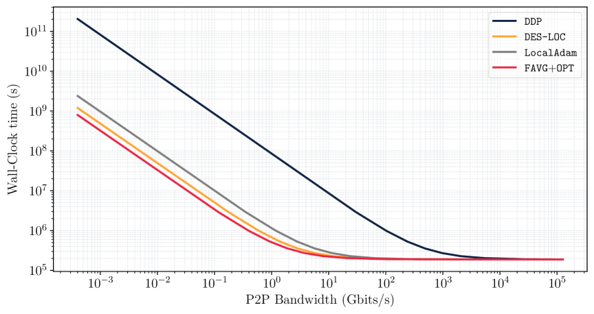
Figure 15: Estimated wall-clock time for training the $1.7$B model with DES-LOC ($K_{x}=256,K_{u}=768,K_{v}=1536$), compared to Local Adam ($K=256$), DDP, and Federated Averaging with persistent optimizer states (FAVG+OPT, $K=256$). At low bandwidth ($<10^{3}$), all communication-efficient methods substantially reduce wall-clock time compared to DDP. DES-LOC closely approaches the maximum efficiency of FAVG+OPT, significantly outperforming Local Adam, which synchronizes all optimizer states frequently. Moreover, DES-LOC maintains stable and convergent training behavior (Fig.˜6). At high bandwidth ($>10^{3}$), DDP becomes competitive or preferable.

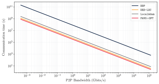
(a)

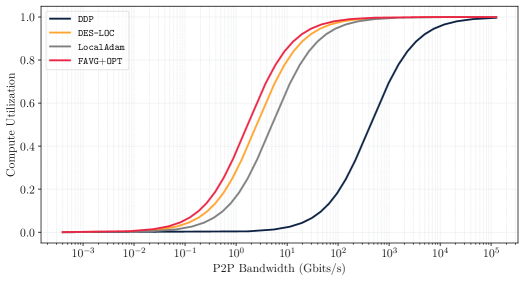
(b)

Figure 16: Communication overhead (a) and GPU utilization (b) for training the $1.7$B model with synchronization periods $K_{x}=256,K_{u}=768,K_{v}=1536$. DES-LOC reduces communication costs by $170\times$ compared to DDP, outperforming the $85\times$ reduction achieved by Local Adam while FAVG+OPT, communicating only parameters, achieves a theoretical maximum reduction ($256\times$). The improved communication efficiency of DES-LOC translates to higher GPU utilization at low bandwidths ($<10^{3}$), significantly improving over DDP and Local Adam.

References

• Allal et al. [2025] L. B. Allal, A. Lozhkov, E. Bakouch, G. M. Blázquez, G. Penedo, L. Tunstall, A. Marafioti, H. Kydlícek, A. P. Lajarín, V. Srivastav, J. Lochner, C. Fahlgren, X. Nguyen, C. Fourrier, B. Burtenshaw, H. Larcher, H. Zhao, C. Zakka, M. Morlon, C. Raffel, and T. Wolf. Smollm2: When smol goes big - data-centric training of a small language model. arXiv preprint arXiv:2502.02737, 2025.
• Arjevani et al. [2023] Y. Arjevani, Y. Carmon, J. C. Duchi, D. J. Foster, N. Srebro, and B. Woodworth. Lower bounds for non-convex stochastic optimization. Mathematical Programming, 199(1-2):165–214, 2023.
• Balles and Hennig [2018] L. Balles and P. Hennig. Dissecting adam: The sign, magnitude and variance of stochastic gradients. In International Conference on Machine Learning (ICML), 2018.
• Ben Allal et al. [2024] L. Ben Allal, A. Lozhkov, G. Penedo, T. Wolf, and L. von Werra. Cosmopedia, February 2024.
• Bisk et al. [2020] Y. Bisk, R. Zellers, R. L. Bras, J. Gao, and Y. Choi. PIQA: reasoning about physical commonsense in natural language. In The Thirty-Fourth AAAI Conference on Artificial Intelligence, AAAI 2020, The Thirty-Second Innovative Applications of Artificial Intelligence Conference, IAAI 2020, The Tenth AAAI Symposium on Educational Advances in Artificial Intelligence, EAAI 2020, New York, NY, USA, February 7-12, 2020, pages 7432–7439. AAAI Press, 2020.
• Brown et al. [2020] T. Brown, B. Mann, N. Ryder, M. Subbiah, J. D. Kaplan, P. Dhariwal, A. Neelakantan, P. Shyam, G. Sastry, A. Askell, S. Agarwal, A. Herbert-Voss, G. Krueger, T. Henighan, R. Child, A. Ramesh, D. Ziegler, J. Wu, C. Winter, C. Hesse, M. Chen, E. Sigler, M. Litwin, S. Gray, B. Chess, J. Clark, C. Berner, S. McCandlish, A. Radford, I. Sutskever, and D. Amodei. Language models are few-shot learners. In Conference on Neural Information Processing Systems (NeurIPS), 2020.
• Charles et al. [2025] Z. Charles, G. Teston, L. Dery, K. Rush, N. Fallen, Z. Garrett, A. Szlam, and A. Douillard. Communication-efficient language model training scales reliably and robustly: Scaling laws for diloco. arXiv preprint arXiv:2503.09799, 2025.
• Chen et al. [2023] X. Chen, C. Liang, D. Huang, E. Real, K. Wang, H. Pham, X. Dong, T. Luong, C. Hsieh, Y. Lu, and Q. V. Le. Symbolic discovery of optimization algorithms. In Conference on Neural Information Processing Systems (NeurIPS), 2023.
• Cheng and Glasgow [2025] Z. Cheng and M. Glasgow. Convergence of distributed adaptive optimization with local updates. In International Conference on Learning Representations (ICLR), 2025.
• Chowdhery et al. [2023] A. Chowdhery, S. Narang, J. Devlin, M. Bosma, G. Mishra, A. Roberts, P. Barham, H. W. Chung, C. Sutton, S. Gehrmann, P. Schuh, K. Shi, S. Tsvyashchenko, J. Maynez, A. Rao, P. Barnes, Y. Tay, N. Shazeer, V. Prabhakaran, E. Reif, N. Du, B. Hutchinson, R. Pope, J. Bradbury, J. Austin, M. Isard, G. Gur-Ari, P. Yin, T. Duke, A. Levskaya, S. Ghemawat, S. Dev, H. Michalewski, X. Garcia, V. Misra, K. Robinson, L. Fedus, D. Zhou, D. Ippolito, D. Luan, H. Lim, B. Zoph, A. Spiridonov, R. Sepassi, D. Dohan, S. Agrawal, M. Omernick, A. M. Dai, T. S. Pillai, M. Pellat, A. Lewkowycz, E. Moreira, R. Child, O. Polozov, K. Lee, Z. Zhou, X. Wang, B. Saeta, M. Diaz, O. Firat, M. Catasta, J. Wei, K. Meier-Hellstern, D. Eck, J. Dean, S. Petrov, and N. Fiedel. Palm: Scaling language modeling with pathways. J. Mach. Learn. Res., 24:240:1–240:113, 2023.
• Clark et al. [2018] P. Clark, I. Cowhey, O. Etzioni, T. Khot, A. Sabharwal, C. Schoenick, and O. Tafjord. Think you have solved question answering? try arc, the AI2 reasoning challenge. CoRR, abs/1803.05457, 2018.
• Douillard et al. [2023] A. Douillard, Q. Feng, A. A. Rusu, R. Chhaparia, Y. Donchev, A. Kuncoro, M. Ranzato, A. Szlam, and J. Shen. Diloco: Distributed low-communication training of language models. arXiv preprint arXiv:2311.08105, 2023.
• Dubey et al. [2024] A. Dubey, A. Jauhri, A. Pandey, A. Kadian, A. Al-Dahle, A. Letman, A. Mathur, A. Schelten, A. Yang, A. Fan, A. Goyal, A. Hartshorn, A. Yang, A. Mitra, A. Sravankumar, A. Korenev, A. Hinsvark, A. Rao, A. Zhang, A. Rodriguez, A. Gregerson, A. Spataru, B. Rozière, B. Biron, B. Tang, B. Chern, C. Caucheteux, C. Nayak, C. Bi, C. Marra, C. McConnell, C. Keller, C. Touret, C. Wu, C. Wong, C. C. Ferrer, C. Nikolaidis, D. Allonsius, D. Song, D. Pintz, D. Livshits, D. Esiobu, D. Choudhary, D. Mahajan, D. Garcia-Olano, D. Perino, D. Hupkes, E. Lakomkin, E. AlBadawy, E. Lobanova, E. Dinan, E. M. Smith, F. Radenovic, F. Zhang, G. Synnaeve, G. Lee, G. L. Anderson, G. Nail, G. Mialon, G. Pang, G. Cucurell, H. Nguyen, H. Korevaar, H. Xu, H. Touvron, I. Zarov, I. A. Ibarra, I. M. Kloumann, I. Misra, I. Evtimov, J. Copet, J. Lee, J. Geffert, J. Vranes, J. Park, J. Mahadeokar, J. Shah, J. van der Linde, J. Billock, J. Hong, J. Lee, J. Fu, J. Chi, J. Huang, J. Liu, J. Wang, J. Yu, J. Bitton, J. Spisak, J. Park, J. Rocca, J. Johnstun, J. Saxe, J. Jia, K. V. Alwala, K. Upasani, K. Plawiak, K. Li, K. Heafield, K. Stone, and et al. The llama 3 herd of models. arXiv preprint arXiv:2407.21783, 2024.
• Hägele et al. [2024] A. Hägele, E. Bakouch, A. Kosson, L. B. Allal, L. von Werra, and M. Jaggi. Scaling laws and compute-optimal training beyond fixed training durations. In Conference on Neural Information Processing Systems (NeurIPS), 2024.
• Hoffmann et al. [2022] J. Hoffmann, S. Borgeaud, A. Mensch, E. Buchatskaya, T. Cai, E. Rutherford, D. de Las Casas, L. A. Hendricks, J. Welbl, A. Clark, T. Hennigan, E. Noland, K. Millican, G. van den Driessche, B. Damoc, A. Guy, S. Osindero, K. Simonyan, E. Elsen, J. W. Rae, O. Vinyals, and L. Sifre. Training compute-optimal large language models. arXiv preprint arXiv:2203.15556, 2022.
• Iacob et al. [2025] A. Iacob, L. Sani, M. Kurmanji, W. F. Shen, X. Qiu, D. Cai, Y. Gao, and N. D. Lane. DEPT: Decoupled embeddings for pre-training language models. In International Conference on Learning Representations (ICLR), 2025.
• Kairouz et al. [2021] P. Kairouz, H. B. McMahan, B. Avent, A. Bellet, M. Bennis, A. N. Bhagoji, K. A. Bonawitz, Z. Charles, G. Cormode, R. Cummings, R. G. L. D’Oliveira, H. Eichner, S. E. Rouayheb, D. Evans, J. Gardner, Z. Garrett, A. Gascón, B. Ghazi, P. B. Gibbons, M. Gruteser, Z. Harchaoui, C. He, L. He, Z. Huo, B. Hutchinson, J. Hsu, M. Jaggi, T. Javidi, G. Joshi, M. Khodak, J. Konečný, A. Korolova, F. Koushanfar, S. Koyejo, T. Lepoint, Y. Liu, P. Mittal, M. Mohri, R. Nock, A. Özgür, R. Pagh, H. Qi, D. Ramage, R. Raskar, M. Raykova, D. Song, W. Song, S. U. Stich, Z. Sun, A. T. Suresh, F. Tramèr, P. Vepakomma, J. Wang, L. Xiong, Z. Xu, Q. Yang, F. X. Yu, H. Yu, and S. Zhao. Advances and open problems in federated learning. Found. Trends Mach. Learn., 14(1-2):1–210, 2021.
• Kaplan et al. [2020] J. Kaplan, S. McCandlish, T. Henighan, T. B. Brown, B. Chess, R. Child, S. Gray, A. Radford, J. Wu, and D. Amodei. Scaling laws for neural language models. CoRR, abs/2001.08361, 2020.
• Karimireddy et al. [2020] S. P. Karimireddy, S. Kale, M. Mohri, S. Reddi, S. Stich, and A. T. Suresh. SCAFFOLD: Stochastic controlled averaging for federated learning. In International Conference on Machine Learning (ICML), 2020.
• Kingma and Ba [2015] D. P. Kingma and J. Ba. Adam: A method for stochastic optimization. In International Conference on Learning Representations (ICLR), 2015.
• Kunstner et al. [2023] F. Kunstner, J. Chen, J. W. Lavington, and M. Schmidt. Noise is not the main factor behind the gap between sgd and adam on transformers, but sign descent might be. In International Conference on Learning Representations (ICLR), 2023.
• Li et al. [2020] S. Li, Y. Zhao, R. Varma, O. Salpekar, P. Noordhuis, T. Li, A. Paszke, J. Smith, B. Vaughan, P. Damania, and S. Chintala. Pytorch distributed: Experiences on accelerating data parallel training. Proc. VLDB Endow., 2020.
• Li et al. [2022] X. Li, B. Karimi, and P. Li. On distributed adaptive optimization with gradient compression. arXiv preprint arXiv:2205.05632, 2022.
• Liu et al. [2024] B. Liu, R. Chhaparia, A. Douillard, S. Kale, A. A. Rusu, J. Shen, A. Szlam, and M. Ranzato. Asynchronous local-sgd training for language modeling. arXiv preprint arXiv:2401.09135, 2024.
• Liu et al. [2020] Y. Liu, Y. Gao, and W. Yin. An improved analysis of stochastic gradient descent with momentum. arXiv preprint arXiv:2007.07989, 2020.
• McMahan et al. [2017] B. McMahan, E. Moore, D. Ramage, S. Hampson, and B. A. y Arcas. Communication-efficient learning of deep networks from decentralized data. In International Conference on Artificial Intelligence and Statistics (AISTATS), 2017.
• Pagliardini et al. [2025] M. Pagliardini, P. Ablin, and D. Grangier. The adEMAMix optimizer: Better, faster, older. In International Conference on Learning Representations (ICLR), 2025.
• Pascanu et al. [2013] R. Pascanu, T. Mikolov, and Y. Bengio. On the difficulty of training recurrent neural networks. In International Conference on Machine Learning (ICML), 2013.
• Penedo et al. [2024] G. Penedo, H. Kydlícek, L. B. Allal, A. Lozhkov, M. Mitchell, C. A. Raffel, L. von Werra, and T. Wolf. The fineweb datasets: Decanting the web for the finest text data at scale. In Conference on Neural Information Processing Systems (NeurIPS), 2024.
• Rajbhandari et al. [2020] S. Rajbhandari, J. Rasley, O. Ruwase, and Y. He. Zero: memory optimizations toward training trillion parameter models. In Proceedings of the International Conference for High Performance Computing, Networking, Storage and Analysis, 2020.
• Reddi et al. [2018] S. J. Reddi, S. Kale, and S. Kumar. On the convergence of adam and beyond. In International Conference on Learning Representations (ICLR), 2018.
• Romero et al. [2022] J. Romero, J. Yin, N. Laanait, B. Xie, M. T. Young, S. Treichler, V. Starchenko, A. Y. Borisevich, A. Sergeev, and M. A. Matheson. Accelerating collective communication in data parallel training across deep learning frameworks. In NSDI, pages 1027–1040. USENIX Association, 2022.
• Sani et al. [2024] L. Sani, A. Iacob, Z. Cao, B. Marino, Y. Gao, T. Paulik, W. Zhao, W. F. Shen, P. Aleksandrov, X. Qiu, and N. D. Lane. The future of large language model pre-training is federated. arXiv preprint arXiv:2405.10853, 2024.
• Sani et al. [2025] L. Sani, A. Iacob, R. L. Zeyu Cao, B. Marino, Y. Gao, W. Zhao, D. Cai, Z. Li, X. Qiu, and N. D. Lane. Photon: Federated llm pre-training. In Eighth Conference on Machine Learning and Systems, 2025.
• Sardana et al. [2024] N. Sardana, J. P. Portes, S. Doubov, and J. Frankle. Beyond chinchilla-optimal: Accounting for inference in language model scaling laws. In International Conference on Machine Learning (ICML), 2024.
• Scao et al. [2022] T. L. Scao, A. Fan, C. Akiki, E. Pavlick, S. Ilic, D. Hesslow, R. Castagné, A. S. Luccioni, F. Yvon, M. Gallé, J. Tow, A. M. Rush, S. Biderman, A. Webson, P. S. Ammanamanchi, T. Wang, B. Sagot, N. Muennighoff, A. V. del Moral, O. Ruwase, R. Bawden, S. Bekman, A. McMillan-Major, I. Beltagy, H. Nguyen, L. Saulnier, S. Tan, P. O. Suarez, V. Sanh, H. Laurençon, Y. Jernite, J. Launay, M. Mitchell, C. Raffel, A. Gokaslan, A. Simhi, A. Soroa, A. F. Aji, A. Alfassy, A. Rogers, A. K. Nitzav, C. Xu, C. Mou, C. Emezue, C. Klamm, C. Leong, D. van Strien, D. I. Adelani, and et al. BLOOM: A 176b-parameter open-access multilingual language model. arXiv preprint arXiv:abs/2211.05100, 2022.
• Sergeev and Balso [2018] A. Sergeev and M. D. Balso. Horovod: fast and easy distributed deep learning in tensorflow. arXiv preprint arXiv:1802.05799, 2018.
• Shoeybi et al. [2019] M. Shoeybi, M. Patwary, R. Puri, P. LeGresley, J. Casper, and B. Catanzaro. Megatron-lm: Training multi-billion parameter language models using model parallelism. CoRR, abs/1909.08053, 2019.
• Smith et al. [2018] S. L. Smith, P. Kindermans, C. Ying, and Q. V. Le. Don’t decay the learning rate, increase the batch size. In International Conference on Learning Representations (ICLR), 2018.
• Stich [2019] S. U. Stich. Local SGD converges fast and communicates little. In International Conference on Learning Representations (ICLR), 2019.
• Su et al. [2024] J. Su, M. H. M. Ahmed, Y. Lu, S. Pan, W. Bo, and Y. Liu. Roformer: Enhanced transformer with rotary position embedding. Neurocomputing, 568:127063, 2024.
• Sutskever et al. [2013] I. Sutskever, J. Martens, G. E. Dahl, and G. E. Hinton. On the importance of initialization and momentum in deep learning. In International Conference on Machine Learning (ICML), 2013.
• Taniguchi et al. [2024] S. Taniguchi, K. Harada, G. Minegishi, Y. Oshima, S. C. Jeong, G. Nagahara, T. Iiyama, M. Suzuki, Y. Iwasawa, and Y. Matsuo. ADOPT: modified adam can converge with any $\beta_{2}$ with the optimal rate. In Conference on Neural Information Processing Systems (NeurIPS), 2024.
• Touvron et al. [2023] H. Touvron, L. Martin, K. Stone, P. Albert, A. Almahairi, Y. Babaei, N. Bashlykov, S. Batra, P. Bhargava, S. Bhosale, D. Bikel, L. Blecher, C. C. Ferrer, M. Chen, G. Cucurull, D. Esiobu, J. Fernandes, J. Fu, W. Fu, B. Fuller, C. Gao, V. Goswami, N. Goyal, A. Hartshorn, S. Hosseini, R. Hou, H. Inan, M. Kardas, V. Kerkez, M. Khabsa, I. Kloumann, A. Korenev, P. S. Koura, M.-A. Lachaux, T. Lavril, J. Lee, D. Liskovich, Y. Lu, Y. Mao, X. Martinet, T. Mihaylov, P. Mishra, I. Molybog, Y. Nie, A. Poulton, J. Reizenstein, R. Rungta, K. Saladi, A. Schelten, R. Silva, E. M. Smith, R. Subramanian, X. E. Tan, B. Tang, R. Taylor, A. Williams, J. X. Kuan, P. Xu, Z. Yan, I. Zarov, Y. Zhang, A. Fan, M. Kambadur, S. Narang, A. Rodriguez, R. Stojnic, S. Edunov, and T. Scialom. Llama 2: Open foundation and fine-tuned chat models, 2023.
• Wang et al. [2021] J. Wang, Z. Charles, Z. Xu, G. Joshi, H. B. McMahan, B. A. y Arcas, M. Al-Shedivat, G. Andrew, S. Avestimehr, K. Daly, D. Data, S. Diggavi, H. Eichner, A. Gadhikar, Z. Garrett, A. M. Girgis, F. Hanzely, A. Hard, C. He, S. Horvath, Z. Huo, A. Ingerman, M. Jaggi, T. Javidi, P. Kairouz, S. Kale, S. P. Karimireddy, J. Konecny, S. Koyejo, T. Li, L. Liu, M. Mohri, H. Qi, S. J. Reddi, P. Richtarik, K. Singhal, V. Smith, M. Soltanolkotabi, W. Song, A. T. Suresh, S. U. Stich, A. Talwalkar, H. Wang, B. Woodworth, S. Wu, F. X. Yu, H. Yuan, M. Zaheer, M. Zhang, T. Zhang, C. Zheng, C. Zhu, and W. Zhu. A field guide to federated optimization. arXiv preprint arXiv:2107.06917, 2021.
• Wortsman et al. [2023] M. Wortsman, T. Dettmers, L. Zettlemoyer, A. Morcos, A. Farhadi, and L. Schmidt. Stable and low-precision training for large-scale vision-language models. In NeurIPS, 2023.
• You et al. [2020] Y. You, J. Li, S. J. Reddi, J. Hseu, S. Kumar, S. Bhojanapalli, X. Song, J. Demmel, K. Keutzer, and C. Hsieh. Large batch optimization for deep learning: Training BERT in 76 minutes. In International Conference on Learning Representations (ICLR), 2020.
• Yu et al. [2019] H. Yu, R. Jin, and S. Yang. On the linear speedup analysis of communication efficient momentum sgd for distributed non-convex optimization. arXiv preprint arXiv:1905.03817, 2019.
• Yuan et al. [2022] K. Yuan, X. Huang, Y. Chen, X. Zhang, Y. Zhang, and P. Pan. Revisiting optimal convergence rate for smooth and non-convex stochastic decentralized optimization. arXiv preprint arXiv:2210.07863, 2022.
• Zellers et al. [2019] R. Zellers, A. Holtzman, Y. Bisk, A. Farhadi, and Y. Choi. Hellaswag: Can a machine really finish your sentence? In A. Korhonen, D. R. Traum, and L. Màrquez, editors, Proceedings of the 57th Conference of the Association for Computational Linguistics, ACL 2019, Florence, Italy, July 28- August 2, 2019, Volume 1: Long Papers, pages 4791–4800. Association for Computational Linguistics, 2019.
• Zhang et al. [2025] H. Zhang, D. Morwani, N. Vyas, J. Wu, D. Zou, U. Ghai, D. Foster, and S. M. Kakade. How does critical batch size scale in pre-training? In The Thirteenth International Conference on Learning Representations, 2025.
• Zhang et al. [2022] Y. Zhang, C. Chen, N. Shi, R. Sun, and Z. Luo. Adam can converge without any modification on update rules. In Conference on Neural Information Processing Systems (NeurIPS), 2022.
• Zhao et al. [2023] Y. Zhao, A. Gu, R. Varma, L. Luo, C. Huang, M. Xu, L. Wright, H. Shojanazeri, M. Ott, S. Shleifer, A. Desmaison, C. Balioglu, P. Damania, B. Nguyen, G. Chauhan, Y. Hao, A. Mathews, and S. Li. Pytorch FSDP: experiences on scaling fully sharded data parallel. Proc. VLDB Endow., 2023.
\mtcsettitle