Renormalizing the Quark-Meson-Diquark Model

Abstract

We present a comprehensive study of the two-flavor Quark–Meson–Diquark (QMD) model by comparing a renormalization approach with a renormalization-group (RG) consistent mean-field formulation based on the functional renormalization group (FRG). The renormalized QMD allows analytical investigations of key quantities such as the zero-temperature diquark gap and the critical temperature for color superconductivity, ultimately reproducing the exact BCS relation in the high-density limit. We carry out the same analysis for different schemes of RG-consistent QMD models. We show that the RG-consistent approach yields a phase diagram and thermodynamic properties qualitatively similar to those of the renormalization model, provided both are embedded within a unified scheme that ensures consistent vacuum properties. In particular, both treatments recover the expected high-density features characterized by the BCS relation and the Stefan–Boltzmann limit. Our results highlight the relevance of renormalization and RG-consistent methods for accurately capturing the thermodynamics of QMD and related effective models with diquark degrees of freedom.

I Introduction

Quantum Chromodynamics (QCD) is the fundamental theory of the strong interaction among quarks and gluons. In the low-energy regime, however, QCD becomes inherently non-perturbative, making direct analytical calculations extremely challenging. Over the years, a variety of non-perturbative tools have been developed to study QCD in this regime. Notably, lattice QCD simulations [1] and continuum functional methods (such as Dyson–Schwinger equations [2] and the functional renormalization group [3]) have provided important insights into the QCD phase structure. Despite these advances, first-principles calculations remain challenging, particularly for the thermodynamics of QCD at finite density, motivating the use of effective models to capture its essential low-energy physics.

Effective models of QCD are designed to respect its symmetries and replicate the dynamics of the full theory, enabling the study of phenomena such as spontaneous chiral symmetry breaking and hadronization within a more manageable framework. Two prominent examples are the Nambu–Jona-Lasinio (NJL) and the quark–meson model, also known as the linear sigma model coupled to quarks. These models dynamically generate constituent quark masses through chiral condensates and successfully capture many qualitative features of low-energy QCD. They have been widely employed to investigate the QCD phase diagram and its transition properties [4, 5, 6].

At high baryon density color superconducting (CSC) phases are expected to emerge, i.e., phases where quarks are paired in so-called diquark condensates [7]. While the quark-meson model and earlier versions of the NJL model account for quark-antiquark condensates only, CSC phases can straightforwardly be described within the NJL model by adding the appropriate quark-quark interactions [8, 9, 4]. Similarly, a natural extension of the quark-meson model to enable the modeling of CSC is the inclusion of diquark degrees of freedom. This leads to the so-called Quark–Meson–Diquark (QMD) model [10, 11], first introduced in the context of two-color QCD [12, 13, 14], whose effective Lagrangian incorporates not only mesonic fields (such as the sigma ($\sigma$) and pions $(\vec{\pi})$, associated with the chiral symmetry) but also explicit complex-valued diquark fields ($\Delta$, $\Delta^{*}$) representing correlated quark–quark and antiquark-antiquark pairs. The diquark fields can condense in the color-antitriplet channel, providing a description of the color-superconducting phase of quark matter [7].

Despite their successes, NJL-type models are non-renormalizable. As a result, a momentum cutoff (or another regularization scheme) must be introduced to handle ultraviolet (UV) divergences, and physical predictions can, in general, depend on the choice of the regularization scheme. In particular, a naïve cutoff regularization can induce significant artifacts, making certain observables unphysically sensitive to the regulator [15].

The QM model, which can be regarded as a bosonized NJL model with Yukawa couplings, is renormalizable. However, when treated with a simple cutoff and without proper renormalization, it may exhibit spurious regulator dependencies, see, e.g., [16]. Over the years, various techniques have been developed to mitigate these issues and ensure proper renormalization-group (RG) behavior in effective models.

One strategy to eliminate cutoff artifacts is renormalization – explicitly incorporating a dependence of the bare model parameters (such as couplings and masses) on the regulator scale so that all divergent contributions are absorbed into redefinitions of these parameters. In practice, this involves the introduction of counterterms to ensure that physical observables remain finite and independent of the UV cutoff eventually. As a renormalizable theory, the QMD model permits a fully renormalized formulation in which all UV divergences are absorbed into the bare parameters of the Lagrangian. This issue was recently discussed in Ref. [17] and explicitly demonstrated using dimensional regularization in Ref. [10] – a scheme often favored for preserving symmetries, particularly Lorentz invariance. At finite temperature and chemical potential, however, Lorentz symmetry is explicitly broken, reducing the advantages of this scheme. In the present work, we instead employ a technically simpler three-momentum cutoff, which yields eventually more tractable expressions.

An alternative and powerful approach is provided by the functional renormalization group (FRG) formalism, pioneered by Wetterich [18], which allows for an RG-consistent formulation of the model. In this FRG-based treatment, a scale-dependent effective action is introduced, with the requirement that physical quantities in the infrared (IR) of the flow remain independent of the chosen regulator cutoff. Such FRG-improved schemes have been applied to low-energy QCD models, see e.g. [19, 20, 17]. In particular, these RG-consistent formulations carefully handle additional divergences that arise at finite chemical potential (often referred to as medium-induced divergences) by adjusting the flow of couplings and potentials accordingly. The QMD model can be analyzed using an RG-consistent mean-field methodology, ensuring that cutoff artifacts are canceled out by flow corrections. It should be noted, however, that RG-consistent methods are inherently scheme-dependent due to the treatment of medium-induced divergences. Different subtraction schemes may yield to variations in the results, including changes in the predicted phase diagram. A comparison between the renormalized formulation of the QMD model and an FRG-based RG-consistent treatment is therefore particularly interesting, as the QMD model serves as a controlled testing ground for directly contrasting these schemes.

In both approaches – introducing cutoff-dependent couplings or employing FRG techniques – the goal is to restore RG consistency, ensuring that the model’s predictions exhibit minimal dependence on arbitrary regularization choices.

In this paper, we present a comprehensive comparison between the renormalized QMD model and an RG-consistent QMD formulation at the mean-field level. First, we implement a straightforward renormalization procedure for the QMD model using a three-dimensional momentum cutoff regularization, yielding a renormalized theory with no residual dependence on the cutoff scale. Second, we formulate an RG-consistent mean-field approximation within the FRG framework: starting from the microscopic QMD action, we integrate out quantum fluctuations down to the infrared scale while maintaining RG invariance of the effective potential.

For a meaningful comparison, we fix the model parameters in both approaches to the same physical vacuum observables – such as the pion mass, decay constant, and vanishing diquark gap at vacuum – ensuring that they describe an identical vacuum state. We then analyze how the predictions of these two treatments diverge away from the vacuum and in particular at finite chemical potential and temperature.

An important advantage of implementing an explicit renormalization procedure (or an RG-consistent approximation) is that it enables us to derive analytical results, providing benchmarks for the model’s predictions under extreme conditions. In particular, we demonstrate that in the high-density limit, both approaches recover the expected BCS relation between the zero-temperature diquark gap, $\Delta(T=0)$, and the critical temperature, $T_{c}$, of the superconducting phase. Furthermore, we verify that as the quark chemical potential $\mu$ increases, both treatments approach the free-quark Stefan–Boltzmann limit for thermodynamic quantities, ensuring consistency with standard thermodynamic expectations. On the other hand we find that, in the QMD model, the diquark gap asymptotically approaches a constant at large $\mu$, whereas in full QCD, the pairing gap is expected to diverge in the limit $\mu\to\infty$ despite the weakening of the attractive interaction at high density [21, 22]. Nonetheless, the ability to obtain analytic high-density results within the QMD framework remains valuable, as it allows us to pinpoint the limitations of the model and identify the missing physics necessary for a more accurate description of dense quark-matter.

The remainder of this paper is organized as follows. In  Section II we introduce the QMD model and its field content, describing the quark, meson, and diquark sectors and introduce the standard regularized mean-field approximation. In Section III, we present the renormalization scheme for the QMD model, demonstrating how divergent vacuum contributions can be absorbed into the couplings and discuss the determination of the model parameters from vacuum observables. Section IV is devoted to the FRG approach and the implementation of the RG-consistent mean-field approximation, with special attention to the treatment of medium-dependent divergences at finite chemical potential. In Section V we present analytical results for the different regularization schemes. In particular, we derive analytically the asymptotic behavior of the diquark condensate and the BCS relation. In Section VI we compare numerical results for the renormalized and RG-consistent approaches, examining the resulting phase diagram and thermodynamic properties such as the diquark gap, critical temperatures, and pressure. Finally, we summarize our findings in Section VII, highlighting the agreements and differences between the two treatments and offering some outlook for future investigations.

II Quark-meson-diquark Model

In this section, we introduce the $N_{f}=2$ quark-meson-diquark model which serves as the foundation of our analysis. This model describes the interaction between the quark fields $q$ and $\bar{q}$ and the effective degrees of freedom associated with the $\sigma$ and $\vec{\pi}$ mesons, as well as the diquark fields $\Delta$ and $\Delta^{*}$. The action of the model in the Euclidean space at finite temperature $\beta=1/T$ is given by

$$S[\bar{q},q,\phi,{\Delta},{\Delta}^{*}]= \int_{0}^{\beta}\!\!dx_{4}\int\!\!d^{3}x\bigg{\{}\bar{q}\left[Z_{q}\left(\not{\partial}-\mu\gamma_{4}\right)+g_{\phi}\left(\sigma+i\gamma_{5}\vec{\pi}\cdot\vec{\tau}\right)\right]q+\frac{1}{2}g_{\Delta}\left(\Delta_{a}\bar{q}\gamma_{5}\tau_{2}i\epsilon_{a}C\bar{q}^{\mathsf{T}}-\Delta_{a}^{*}q^{\mathsf{T}}C\gamma_{5}\tau_{2}i\epsilon_{a}q\right)$$

$$+\frac{Z_{\phi}}{2}(\partial_{\mu}\phi)(\partial_{\mu}\phi)+Z_{\Delta}(\partial_{\mu}+2\mu\delta_{\mu 4})\Delta_{a}^{*}(\partial_{\mu}-2\mu\delta_{\mu 4})\Delta_{a}+U(\phi^{2},|\Delta|^{2})-c\sigma\bigg{\}}\;.$$ (1)

Here, the quark fields $q$ and $\bar{q}$ are understood as vectors in color, flavor and Dirac space. The mesonic fields are grouped into the $O(4)$-symmetric chiral field $\phi^{\mathsf{T}}=(\sigma,\vec{\pi}^{\mathsf{T}})$ which provides a convenient basis for constructing the chirally invariant quantity $\phi^{2}=\sigma^{2}+\vec{\pi}^{\,2}$. The complex-valued diquark fields $\Delta$ and $\Delta^{*}$ are understood as vectors in color space and their components $\Delta_{a}$ and $\Delta^{*}_{a}$ carry a color index $a=1,2,3$.

Throughout this work, we generally omit field indices for readability, except for the diquark fields, where the color indices are always shown explicitly. Additionally, we define the diquark invariant as $|\Delta|^{2}=|\Delta_{1}|^{2}+|\Delta_{2}|^{2}+|\Delta_{3}|^{2}$. The Euclidean $\gamma$-matrices are defined such that $\{\gamma_{\mu},\gamma_{\nu}\}=2\delta_{\mu\nu}$ and the charge conjugation matrix reads $C=\gamma_{2}\gamma_{4}$. We also introduced the fully antisymmetric tensor in color space $(\epsilon_{a})_{bc}=\epsilon_{abc}$ and the three Pauli matrices $\tau_{i}$ acting in flavor space.

In Eq. 1, the kinetic terms of the quark, meson and diquark field are included with their associated wave function renormalizations $Z_{q}$, $Z_{\phi}$ and $Z_{\Delta}$. In particular, note the structure of the diquark kinetic term, which explicitly couples to the chemical potential $\mu$ because the diquark field carries a nonzero $U(1)_{B}$ charge.

We collect all bosonic interaction terms in a potential $U(\phi^{2},|\Delta|^{2})$, which depends only on the chiral invariant $\phi^{2}$ and the diquark invariant $|\Delta|^{2}$. The most general form of this potential, which includes all relevant and marginal couplings, is given by

$$\begin{split}&U(\phi^{2},|\Delta|^{2})=\frac{1}{2}m^{2}_{\phi}\phi^{2}+\frac{1}{4}\lambda_{\phi}\phi^{4}\\ &\quad+m^{2}_{\Delta}|\Delta|^{2}+\lambda_{\Delta}|\Delta|^{4}+\frac{1}{2}\lambda_{\text{mix}}\phi^{2}|\Delta|^{2}\;.\end{split}$$ (2)

In practical applications, it is common to omit some of the couplings due to the lack of physical observables sensitive to diquark pairing, which limits constraints on these couplings. A typical and simple approximation sets $\lambda_{\Delta}=\lambda_{\text{mix}}=0$. However, as we will show in Section III, all of these couplings are essential for renormalization. We revisit the issue of missing constraints in Section VI.1.

Regularized mean-field approximation

A common approach for studying the model’s thermodynamic properties is the mean-field approximation, where the bosonic fields are assumed to take constant field configurations: $\phi^{\mathsf{T}}=(\sigma,\vec{0}^{\,\mathsf{T}})$ and $\Delta_{a}=\Delta\delta_{a3}$ with $\sigma\in\mathbb{R}$ and $\Delta\in\mathbb{R}$. Note that in a slight abuse of notation we use the same symbol for the homogeneous field configuration and for the space-time dependent field. Then, neglecting all bosonic fluctuations in the path integral, the effective thermodynamic potential of the model can be computed as

$$\Omega_{\text{reg}}^{\text{eff}}(\sigma,\Delta)=U(\sigma^{2},\Delta^{2})-c\sigma-4Z_{\Delta}\mu^{2}\Delta^{2}+L_{\Lambda}(\sigma,\Delta)\;,$$ (3)

where

$$L_{\Lambda}(\sigma,\Delta)=-2N_{f}\int_{|\vec{p}|<\Lambda}\bigg{\{}E_{q}^{+}+E_{q}^{-}+\epsilon_{q}$$ (4)

$$\quad+2T\ln\left(1+e^{-E_{q}^{+}/T}\right)+2T\ln\left(1+e^{-E_{q}^{-}/T}\right)$$

$$\quad+T\ln\left(1+e^{-\epsilon_{q}^{+}/T}\right)+T\ln\left(1+e^{-\epsilon_{q}^{-}/T}\right)\bigg{\}}\;,$$

stands for the quark loop contribution with the dispersion relations

$$E_{q}^{\pm}=\sqrt{{\epsilon_{q}^{\pm}}^{2}+\Delta_{\text{gap}}^{2}}\;,$$ (5)

and

$$\epsilon_{q}^{\pm}=\epsilon_{q}\pm\mu\quad\text{with }\quad\epsilon_{q}=\sqrt{\vec{p}^{\,2}+m_{q}^{2}}\;.$$ (6)

The quark mass $m_{q}$ and the Fermi-surface gap $\Delta_{\text{gap}}$ are related to the homogeneous field configurations through

$$m_{q}=g_{\phi}\sigma\quad\text{and}\quad\Delta_{\text{gap}}=g_{\Delta}\Delta\;.$$ (7)

In general, we use a short-hand notation for momentum integrals, where the integral index specifies any possible cutoffs

$$\int_{\vec{p}}\equiv\int\!\!\frac{d^{3}p}{(2\pi)^{3}}\;,\quad\text{and}\quad\int_{|\vec{p}|<\Lambda}\equiv\int\!\!\frac{d^{3}p}{(2\pi)^{3}}\theta(\Lambda^{2}-\vec{p}^{\,2})\;.$$ (8)

Thus, the effective potential Eq. 3 consists of the tree-level bosonic potential with the explicit symmetry breaking term, a quadratic diquark contribution from the diquark kinetic term that still depends on the chemical potential, and a quark loop contribution. The divergent quark loop is regularized with a three-momentum cutoff, $|\vec{p}|<\Lambda$. We refer to Eq. 3 as the regularized mean-field approximation (regMFA) and use the subscript reg accordingly.

Note that in obtaining Eq. 3 we implicitly chose to set $Z_{q}=1$. At the mean-field level, the quark wave function renormalization receives no loop contribution and only contributes through a rescaling of the Yukawa couplings $g_{\phi}$ and $g_{\Delta}$. As such any dependency on $Z_{q}$ can be safely removed by a rescaling of $g_{\phi}$ and $g_{\Delta}$, which is fully equivalent to choosing $Z_{q}=1$ in Eq. 1. This is in contrast to the meson and diquark wave function renormalizations which receive a loop contribution. As we only consider homogeneous condensates, the meson wave function $Z_{\phi}$ does not contribute to the effective potential and can safely be ignored. However, the diquark wave function renormalization $Z_{\Delta}$ contributes to the effective potential and must, without further approximations, be considered.

The three-momentum cutoff regularization scheme is often used in the literature due to its simplicity and the fact that at finite $T$ and $\mu$ the Lorentz symmetry is already explicitly broken. Only the $T=0$ contribution of the quark loop diverges, as can be seen from the asymptotic expansion

$$\begin{split}&L_{\Lambda}(\sigma,\Delta)\underset{\Lambda\to\infty}{\simeq}{}-\frac{3}{2\pi^{2}}{\Lambda}^{4}-\frac{\left(3m_{q}^{2}+2\Delta^{2}_{\text{gap}}\right)}{2\pi^{2}}{\Lambda}^{2}\\ &+\left(\frac{3m_{q}^{4}}{4\pi^{2}}+\frac{m_{q}^{2}\Delta_{\text{gap}}^{2}}{\pi^{2}}+\frac{\Delta_{\text{gap}}^{4}}{2\pi^{2}}-\mu^{2}\frac{2\Delta_{\text{gap}}^{2}}{\pi^{2}}\right)\ln\Lambda\;.\end{split}$$ (9)

Note in particular the presence of a $\mu^{2}$ divergence, which we call a medium divergence.

The regularized effective potential Eq. 3 suffers from cutoff artifacts due to the absence of high-momentum modes $|\vec{p}|>\Lambda$. A straightforward yet naïve solution is to choose $\Lambda$ much larger than any physical scale in the system. However, this procedure presents two difficulties.

The first difficulty is technical: the vacuum and medium contributions to the effective potential diverge as $\Lambda\to\infty$ (see Eq. 9). Due to these divergences, fixing the bare parameters as $\Lambda\to\infty$ becomes a fine-tuning problem. The renormalization of the model is the procedure that resolves this fine-tuning issue.

The second difficulty is conceptual: in non-renormalizable models like the NJL model, the cutoff $\Lambda$ is an intrinsic parameter - similar to the bare couplings - and is chosen to reproduce vacuum phenomenology. As a result, it may be impossible to eliminate all cutoff artifacts by simply tuning $\Lambda$. RG-consistency offers a way to addresss this issue, enabling the removal of cutoff artifacts in both renormalizable and non-renormalizable models [20, 17]. We are thus faced with two approaches that aim to achieve the same goal. It is therefore natural to compare them directly.

In the following Section III, we present a straightforward renormalization procedure to eliminate the cutoff dependence. Then, Section IV briefly reviews the RG-consistency approach introduced in Ref. [20] and discusses how it handles medium divergences. Finally, in Sections V and VI, we compare the predictions of the two methods using both analytical and numerical results.

III Renormalized Approach

In the renormalized approach, the bare parameters are assumed to depend on the cutoff scale $\Lambda$ such that the effective potential remains finite as $\Lambda\to\infty$. To detail this, we derive in Section III.1 the asymptotic behavior of the couplings required for finiteness of the potential. In Section III.2, we present an explicit strategy for implementing the renormalized mean-field approximation.

III.1 Asymptotic expansion

Vacuum parameters	Physical interpretation
$\tilde{f}_{\pi}=\sigma_{\text{vac}}$	pion decay constant
$\tilde{m}_{\sigma}^{2}=\displaystyle\left.\left(\partial_{\sigma}^{2}\,\Omega^{\text{eff}}\right)\right|_{\text{vac}}$	$\sigma$ mass
$\tilde{m}_{\Delta}^{2}=\displaystyle\frac{1}{2}\left.\left(\partial_{\Delta}^{2}\,\Omega^{\text{eff}}\right)\right|_{\text{vac}}$	diquark mass
$\tilde{\lambda}_{\text{mix}}=\displaystyle\frac{1}{2}\left.\left(\partial_{\sigma}^{2}\,\partial_{\Delta}^{2}\,\Omega^{\text{eff}}\right)\right|_{\text{vac}}$	$\Delta$–$\sigma$ scattering amplitude
$\tilde{\lambda}_{\Delta}=\displaystyle\frac{1}{24}\left.\left(\partial_{\Delta}^{4}\,\Omega^{\text{eff}}\right)\right|_{\text{vac}}$	(anti)diquark–(anti)diquark scattering amplitude
$\tilde{Z}_{\Delta}=\displaystyle-\frac{1}{16}\left.\left(\partial_{\mu}^{2}\,\partial_{\Delta}^{2}\,\Omega^{\text{eff}}\right)\right|_{\text{vac}}$	diquark wave function renormalization

Table 1: Vacuum parameters and their definitions in terms of the effective action, along with their physical interpretation (in vacuum). The subscript $"{\text{vac}}"$ denotes evaluation at $\sigma=\tilde{f}_{\pi}$ and $\Delta=0$ in vacuum.

We begin by noting that all divergent contributions to the effective potential take the form shown in Eq. 9. By rewriting this expression in terms of the condensates and comparing it to the various bare couplings in $U(\phi^{2},|\Delta|^{2})$, we find that all purely bosonic bare couplings are required to absorb the divergences - except for the medium divergence, which can be handled via the wave function renormalization of the diquarks.

Promoting all couplings and the diquark wave function renormalization in the regularized potential $\Omega_{\text{reg}}^{\text{eff}}$, Eq. 3, to functions of the cutoff $\Lambda$, the renormalized effective potential $\Omega_{\text{ren}}^{\text{eff}}$ is eventually obtained by taking the limit $\Lambda\to\infty$. An asymptotic expansion of the renormalized potential together with Eq. 9 then yields

$$\Omega_{\text{ren}}^{\text{eff}}(\sigma,\Delta)\underset{\Lambda\to\infty}{\simeq}\frac{1}{2}\bigg{[}\lambda_{\text{mix}}(\Lambda)+\frac{2g^{2}_{\phi}g^{2}_{\Delta}}{\pi^{2}}\ln\Lambda\bigg{]}\sigma^{2}\Delta^{2}$$

$$+\frac{1}{2}\bigg{[}m^{2}_{\phi}(\Lambda)-\frac{3g_{\phi}^{2}}{\pi^{2}}{\Lambda}^{2}\bigg{]}\sigma^{2}+\frac{1}{4}\bigg{[}\lambda_{\phi}(\Lambda)+\frac{3g_{\phi}^{4}}{\pi^{2}}\ln\Lambda\bigg{]}\sigma^{4}$$

$$+\bigg{[}m^{2}_{\Delta}(\Lambda)-\frac{g_{\Delta}^{2}}{\pi^{2}}{\Lambda}^{2}\bigg{]}\Delta^{2}+\bigg{[}\lambda_{\Delta}(\Lambda)+\frac{g^{4}_{\Delta}}{2\pi^{2}}\ln\Lambda\bigg{]}\Delta^{4}$$

$$-4\bigg{[}Z_{\Delta}(\Lambda)+\frac{g_{\Delta}^{2}}{2\pi^{2}}\ln\Lambda\bigg{]}\mu^{2}\Delta^{2}-\frac{3}{2\pi^{2}}{\Lambda}^{4}\;,$$ (10)

From Section III.1, we conclude that maintaining a finite effective potential as $\Lambda\to\infty$ requires the bare couplings to scale with $\Lambda$ as follows:

$$m_{\phi}^{2}(\Lambda) =\frac{3g_{\phi}^{2}}{\pi^{2}}\Lambda^{2}+\mathcal{O}(1)\;,$$ (11)

$$m_{\Delta}^{2}(\Lambda) =\frac{g_{\Delta}^{2}}{\pi^{2}}\Lambda^{2}+\mathcal{O}(1)\;,$$ (12)

$$Z_{\Delta}(\Lambda) =-\frac{g_{\Delta}^{2}}{2\pi^{2}}\ln\Lambda+\mathcal{O}(1)\;,$$ (13)

$$\lambda_{\phi}(\Lambda) =-\frac{3g_{\phi}^{4}}{\pi^{2}}\ln\Lambda+\mathcal{O}(1)\;,$$ (14)

$$\lambda_{\text{mix}}(\Lambda) =-\frac{2g_{\phi}^{2}g_{\Delta}^{2}}{\pi^{2}}\ln\Lambda+\mathcal{O}(1)\;,$$ (15)

$$\lambda_{\Delta}(\Lambda) =-\frac{g_{\Delta}^{4}}{2\pi^{2}}\ln\Lambda+\mathcal{O}(1)\;.$$ (16)

The remaining parameters $g_{\phi}$, $g_{\Delta}$, and $c$ stay finite, as they do not receive loop corrections at mean-field level, and can therefore be treated as cutoff-independent.

III.2 Vacuum matching scheme

We now outline a concrete strategy to fix the model parameters. In general, determining all couplings and their cutoff dependence requires a sufficient number of constraints, typically obtained by fitting a suitable set of vacuum parameters. If the focus is limited to the homogeneous phase diagram and one aims to avoid fitting observables sensitive to the momentum dependence of correlation functions (such as pole masses), the mesonic wave function renormalization $Z_{\phi}$ can be neglected. In contrast, the diquark wave function renormalization $Z_{\Delta}$ must be retained, as it enters the effective potential explicitly through its coupling to the chemical potential, as previously noted.

The importance of wave function renormalization for the renormalizability of such effective models at finite density was recently emphasized in Ref. [23]. In the context of the two-flavor quark-meson model at finite isospin density, it was shown within an RG-invariant mean-field approximation that, once a single RG-invariant scale is matched to lattice data, the resulting equation of state and phase diagram agree quantitatively with modern lattice simulations over a broad range of $\mu_{I}$.

As already mentioned, $g_{\phi}$, $g_{\Delta}$ and $c$ receive no loop contributions in MFA. They can therefore be fixed directly, without requiring corresponding vacuum parameters. This leaves six couplings from Eqs. 11 to 16 that must be determined. To illustrate the procedure, we fix them using a set of vacuum parameters – a process we refer to as the vacuum matching scheme. The chosen set of parameters is

$$\mathcal{P}_{\text{vac}}=\{\tilde{f}_{\pi},\tilde{m}_{\sigma}^{2},\tilde{m}_{\Delta}^{2},\tilde{Z}_{\Delta},\tilde{\lambda}_{\text{mix}},\tilde{\lambda}_{\Delta}\}\;.$$ (17)

In Table 1, we list the vacuum parameters, their definitions in terms of the effective action, and their physical interpretations. It is worth noting that this choice of parameters is not unique – alternative sets of vacuum parameters could be used. In particular, no parameter is directly associated with $\lambda_{\phi}$, which will instead be fixed through a combination of $\tilde{f}_{\pi}$ and $\tilde{m}_{\sigma}^{2}$, as discussed in Appendix A.

Note that the diquark wave function renormalization, $Z_{\Delta}$, is associated with single particle states and, in this regard, is not directly linked to any physical observable. One can always fix $Z_{\Delta}$ to an arbitrary constant at a fixed scale, which in turn rescales the fields and consequently modifies the values of other model couplings. Here, we choose to fix this parameter in vacuum. In contrast, the remaining parameters can be related to physical observables involving multi-particle states that are, for example, realized through certain scattering or decay processes. To this end, we define a set of vacuum parameters that can be associated with these physical quantities.

The pion decay constant is directly related to the chiral condensate in vacuum

$$\tilde{f}_{\pi}=\langle\sigma\rangle_{\text{vac}}\ ,$$ (18)

which is determined as the solution of the gap equation evaluated for vanishing diquark condensate

$$\frac{\partial\Omega^{\text{eff}}_{\text{ren}}(\sigma,\Delta=0)}{\partial\sigma}=0\;.$$ (19)

For $\Delta=0$ we can use Eq. 3 and obtain

$$m_{\phi}^{2}\tilde{f}_{\pi}+\lambda_{\phi}\tilde{f}_{\pi}^{3}+\frac{\partial L_{\Lambda}(\sigma,\Delta=0)}{\partial\sigma}-c=0\;.$$ (20)

With the definitions of the remaining vacuum parameters, one can derive a linear system of equations that allows one to express the bare parameters in terms of vacuum quantities. Substituting these expressions into the effective potential and subsequently taking the limit $\Lambda\to\infty$ yields a renormalized form of the effective potential. The details of this procedure are presented in Appendix A. The renormalized potential takes the following form

$$\Omega^{\text{eff}}_{\text{ren}}(\sigma,\Delta)={} U_{\text{ren}}(\sigma^{2},\Delta^{2})-c\sigma-4\tilde{Z}_{\Delta}\Delta^{2}\mu^{2}$$

$$+L_{\text{ren}}(\sigma,\Delta)\;,$$ (21)

where $U_{\text{ren}}$ is the renormalized potential contribution, now expressed in terms of the vacuum parameters as

$$U_{\text{ren}}(\sigma^{2},\Delta^{2})=\tilde{\lambda}_{\Delta}\Delta^{4}+\Bigl{(}-\frac{\tilde{m}_{\sigma}^{2}}{4}+\frac{3c}{4\tilde{f}_{\pi}}\Bigr{)}\sigma^{2}$$

$$\quad+\Bigl{(}-\frac{c}{8\tilde{f}_{\pi}^{3}}+\frac{\tilde{m}_{\sigma}^{2}}{8\tilde{f}_{\pi}^{2}}\Bigr{)}\sigma^{4}+\frac{1}{2}\tilde{\lambda}_{\text{mix}}\sigma^{2}\Delta^{2}$$

$$\quad+\Bigl{(}\tilde{m}_{\Delta}^{2}-\frac{1}{2}\tilde{\lambda}_{\text{mix}}\tilde{f}_{\pi}^{2}\Bigr{)}\Delta^{2}\;,$$ (22)

and $L_{\text{ren}}(\sigma,\Delta)$ represents the renormalized loop contribution

$$L_{\text{ren}}(\sigma,\Delta)=2N_{f}\int_{\vec{p}}\bigg{\{}3p+\frac{\Delta_{\text{gap}}^{2}\mu^{2}}{\epsilon_{q,\text{vac}}^{3}}-\frac{\Delta_{\text{gap}}^{4}}{4\epsilon_{q,\text{vac}}^{3}}+\frac{\Delta_{\text{gap}}^{2}}{2\epsilon_{q,\text{vac}}^{5}}p^{2}\left(2p^{2}+5m_{q,\text{vac}}^{2}\right)-\frac{\Delta_{\text{gap}}^{2}m_{q}^{2}}{2\epsilon_{q,\text{vac}}^{5}}\left(p^{2}-2m_{q,\text{vac}}^{2}\right)$$

$$\quad+\frac{3m_{q}^{2}}{4\epsilon_{q,\text{vac}}^{3}}\left(2p^{2}+3m_{q,\text{vac}}^{2}\right)-\frac{3m_{q}^{4}}{8\epsilon_{q,\text{vac}}^{3}}-E_{q}^{+}-E_{q}^{-}-\epsilon_{q}$$

$$\quad-2T\ln\left(1+e^{-E_{q}^{+}/T}\right)-2T\ln\left(1+e^{-E_{q}^{-}/T}\right)-T\ln\left(1+e^{-\epsilon_{q}^{+}/T}\right)-T\ln\left(1+e^{-\epsilon_{q}^{-}/T}\right)\bigg{\}}\;.$$ (23)

It includes both the standard loop contribution and the additional counterterm contribution arising from the bare parameters. This results in a finite expression for the effective potential in the limit $\Lambda\to\infty$.

Using this, we can define the gap equations

$$\left.\frac{\partial\Omega^{\text{eff}}_{\text{ren}}(\sigma,\Delta;T,\mu)}{\partial\sigma}\right|_{{\bar{\sigma},\bar{\Delta}}}=0\;,$$ (24a)

$$\left.\frac{\partial\Omega^{\text{eff}}_{\text{ren}}(\sigma,\Delta;T,\mu)}{\partial\Delta}\right|_{{\bar{\sigma},\bar{\Delta}}}=0\;.$$ (24b)

By solving these two equations simultaneously we get the physical gap solutions $\bar{\sigma}(T,\mu)$, and $\bar{\Delta}(T,\mu)$ and we get the thermodynamic potential by inserting these solutions back into the effective potential. What is now missing are the values of the vacuum parameters we have introduced. We will come back to them in Section VI.1.

IV RG-consistent Mean-field Approximation

We now adopt an alternative perspective on the mean-field approximation which is based on the functional renormalization group (FRG). First we demonstrate how the FRG framework reproduces the regMFA. We then use this approach to construct RG-consistent (RGC) approximations, with a particular focus on the treatment of medium divergences. This leads to alternative forms of the effective potential, which we compare with the renormalized approach in Sections V and VI.

IV.1 FRG and MFA

The FRG is rooted in the Wilsonian formulation of the renormalization group in quantum field theory. The Wilsonian coarse-graining procedure is captured by a functional differential equation for an effective action. In this work, we employ the Wetterich equation [18], where the central object is the scale-dependent one-particle irreducible effective action $\Gamma_{k}$ with the infrared (IR) cutoff scale $k$. For a purely fermionic theory, the Wetterich equation takes the form

$$\partial_{t}\Gamma_{k}=-\frac{1}{2}\text{Tr}\left[\left(\Gamma^{(2)}_{k}+R_{k}\right)^{-1}\partial_{t}R_{k}\right]\;,$$ (25)

where $\partial_{t}=k\partial_{k}$ denotes the derivative with respect to the dimensionless scale $t=\log(k/\Lambda)$ with the UV cutoff scale $\Lambda$. In Eq. 25, $\Gamma^{(2)}_{k}$ denotes the full two-point function (i.e., the inverse full propagator) for the fermion fields. With the superfield $\Psi^{\mathsf{T}}=(q^{\mathsf{T}},\bar{q})$, it is defined in momentum space as

$$\Gamma^{(2)}_{k}=\frac{\delta^{2}\Gamma_{k}}{\delta\Psi^{\mathsf{T}}(p)\delta\Psi(p)}\ .$$ (26)

The trace Tr in Eq. 25 runs over all relevant spaces, including momentum, color, flavor, and Dirac spaces on which the fermionic fields are defined. The regulator function $R_{k}(p)$ implements the Wilsonian coarse-graining procedure within the path-integral formulation by acting as a scale-dependent mass term. In this work, we employ the sharp three-dimensional regulator function for fermions [26], given by

$$R_{k}(p)=i\not{\vec{p}}\,\left(\frac{1}{\theta(\vec{p}^{\,2}-k^{2})}-1\right)\;,$$ (27)

which renders momentum modes with $p<k$ infinitely massive, while vanishing for $p>k$. This choice is particularly convenient, as it leads to an expression for the effective potential that coincides with the result obtained in the regMFA using a three-momentum cutoff, as shown in Eq. 3.

Solving the Wetterich equation Eq. 25 with the initial condition $\Gamma_{\Lambda}$ at the UV scale $k=\Lambda$ yields the full effective action $\Gamma=\Gamma_{k=0}$ in the infrared limit. In general, $\Gamma_{k}$ admits an infinite expansion in terms of effective operators, rendering the exact treatment of the effective action intractable without suitable truncations.

To recover the MFA results, we employ the following ansatz for the effective action of the quark-meson-diquark model in Euclidean space

$$\qquad\Gamma_{k}=\int_{0}^{\beta}\!\!dx_{4}\int\!\!d^{3}x\bigg{\{}\bar{q}\left[\not{\partial}-\mu\gamma_{4}+g_{\phi}\sigma\right]q$$ (28)

$$+\frac{1}{2}g_{\Delta}\Delta\left(\bar{q}\gamma_{5}\tau_{2}i\epsilon_{3}C\bar{q}^{\mathsf{T}}-q^{\mathsf{T}}C\gamma_{5}\tau_{2}i\epsilon_{3}q\right)+\Omega_{k}^{\text{eff}}(\sigma,\Delta)\bigg{\}}\;,$$

where $\sigma$ and $\Delta$ denote the homogeneous background fields associated with the scalar $\sigma$ and the diquark $\Delta_{3}$ channels, respectively. The scale-dependent effective potential $\Omega_{k}^{\text{eff}}(\sigma,\Delta)$ is treated as a general function of $\sigma$ and $\Delta$. In the infrared limit, it corresponds to the thermodynamic effective potential

$$\Omega^{\text{eff}}(\sigma,\Delta)\equiv\frac{\Gamma_{k=0}(\sigma,\Delta)}{\beta V}=\Omega_{k=0}^{\text{eff}}(\sigma,\Delta)\;,$$ (29)

where $V$ denotes the three-dimensional spatial volume. At the UV scale $k=\Lambda$, we initialize the flow with the polynomial form

$$\Omega_{k=\Lambda}^{\text{eff}}(\sigma,\Delta)=U(\sigma^{2},\Delta^{2})-4Z_{\Delta}\mu^{2}\Delta^{2}-c\sigma\;,$$ (30)

which is consistent with the classical action of the quark-meson-diquark model in Eq. 1.

Next, we observe that for the truncation Eq. 28, the inverse two-point function is independent of the RG scale $k$ and coincides with the second derivative of the classical action given in Eq. 1,

$$\Gamma^{(2)}_{k}=S^{(2)}\;,$$ (31)

where $S^{(2)}$ is defined analogously to Eq. 26. This identification lies at the heart of the mean-field approximation and allows the Wetterich equation to be rewritten as

$$\partial_{k}\Gamma_{k}={} -\frac{1}{2}\;\text{Tr}\left[\left(S^{(2)}+R_{k}\right)^{-1}\partial_{k}R_{k}\right]$$

$$={} -\frac{1}{2}\partial_{k}\;\text{Tr}\left[\ln\left(S^{(2)}+R_{k}\right)\right]\;.$$ (32)

With the truncation Eq. 28, we obtain the flow equation for the effective potential

$$\partial_{k}\Omega_{k}^{\text{eff}}(\sigma,\Delta)=\partial_{k}f_{k}(\sigma,\Delta)\;,$$ (33)

where we introduce the shorthand notation

$$f_{k}=-\frac{1}{\beta V}\frac{1}{2}\;\text{Tr}\left[\ln\left(S^{(2)}+R_{k}\right)\right]\;.$$ (34)

Evaluating the trace over flavor, color and Dirac indices, and performing the Matsubara sums in Eq. 34, one obtains

$$f_{k}(\sigma,\Delta)=-L_{k}(\sigma,\Delta)\;,$$ (35)

where $L_{k}(\sigma,\Delta)$ is defined in Eq. 4.

To derive the infrared mean-field potential, we integrate Eq. 33 from $k=\Lambda$ to $k=0$ and recover the regularized effective potential Eq. 3

$$\Omega^{\text{eff}}_{\text{reg}}(\sigma,\Delta)=\Omega_{\Lambda}^{\text{eff}}(\sigma,\Delta)+L_{\Lambda}(\sigma,\Delta)\;,$$ (36)

where we have used $L_{k=0}(\sigma,\Delta)=0$.

Lastly, we remark that the mean-field flow Section IV.1 with the sharp momentum regulator Eq. 27 can be understood as a mapping that directly relates the RG scale $k$ to the UV cutoff scale $\Lambda$. With this in mind, one can alternatively derive the scale dependence of the couplings, the $\beta$-functions, directly from the Wetterich equation by solving their associated flow equations. This procedure reproduces the scale dependency of the couplings in Eqs. 11 to 16 and is explicitly demonstrated in Appendix B.

In the following, we extend this analysis by utilizing the FRG flow to eliminate cutoff artifacts, building on the concept of RG-consistency [20]. In particular, we focus on the treatment of medium-divergences within this framework.

IV.2 RG-consistency of the QMD model

The concept of RG-consistency was introduced in Ref. [20] and has recently been discussed in the context of the $N_{f}=3$ NJL model in Ref. [17]. It requires that the full quantum effective action $\Gamma$ remains independent of the explicit cutoff dependence of $\Gamma_{\Lambda}$,

$$\Lambda\frac{\mathrm{d}\Gamma}{\mathrm{d}\Lambda}=0\;.$$ (37)

In practice, however, this property is not automatically guaranteed if external scales of the theory, such as the temperature or the quark chemical potential, approach the cutoff scale $\Lambda$.

This problem can be overcome using the FRG. The idea is most easily explained for the NJL model [17]. Suppose the initial conditions are originally given by the effective potential $\Omega_{\Lambda^{\prime}}^{\text{eff}}(\sigma,\Delta)$ at some fixed scale $\Lambda^{\prime}$, e.g., obtained from a vacuum fit at this cutoff scale. Then, by formally integrating the flow in vacuum upward to some higher scale $k=\Lambda>\Lambda^{\prime}$, one can construct a modified initial condition for the effective potential, $\Omega_{\Lambda}^{\text{eff}}(\sigma,\Delta)$, which in vacuum leads to the same infrared effective potential. However, flowing downward from $k=\Lambda$ to $k=0$ yields an RG-consistent effective potential $\Omega_{k=0}^{\text{eff}}(\sigma,\Delta)$ even in the presence of finite external scales, provided that $\Lambda$ is much larger than these scales (e.g., $\Lambda\gg T,\mu$).

For the QMD model, the general idea is the same. A small but important difference is that here the effective potential at the initial UV scale (which from now on we will always call $\Lambda^{\prime}$) contains an explicitly $\mu$-dependent term, see Eq. 30. This term, which is not present in the NJL model, originates from the kinetic energy of the diquarks and is essential for the renormalizability of the QMD model. In the following we therefore explicitly separate it from the pure vacuum initial condition by writing

$$\Omega_{\Lambda^{\prime}}^{\text{eff}}(\sigma,\Delta;\mu)=\Omega_{\Lambda^{\prime}}^{\text{eff}}(\sigma,\Delta)-4Z_{\Delta}\mu^{2}\Delta^{2},$$ (38)

where

$$\Omega_{\Lambda^{\prime}}^{\text{eff}}(\sigma,\Delta)\equiv\Omega_{\Lambda^{\prime}}^{\text{eff}}(\sigma,\Delta;\mu=0)=U(\sigma^{2},\Delta^{2})-c\sigma$$ (39)

is a $T$- and $\mu$-independent starting point, similar to the UV initial condition in the NJL model.

From this, the RG-consistent initial effective potential at $k=\Lambda$, $\Omega_{\text{rgc},\Lambda}^{\text{eff}}$, can be constructed by integrating the mean-field flow, Eq. 33, upward from $\Lambda^{\prime}$ to $\Lambda$,

$$\Omega_{\text{rgc},\Lambda}^{\text{eff}}(\sigma,\Delta;\mu)$$

$$\quad=\Omega_{\Lambda^{\prime}}^{\text{eff}}(\sigma,\Delta)-4Z_{\Delta}\mu^{2}\Delta^{2}+\mathcal{F}_{\Lambda^{\prime}\to\Lambda}(\sigma,\Delta;0,0)\;,$$ (40)

with the $\mu$-dependent but scale independent $Z_{\Delta}$ term inherited from Eq. 38 and the flow integral

$$\mathcal{F}_{\Lambda^{\prime}\to\Lambda}(\sigma,\Delta;T,\mu)= \int\limits_{\Lambda^{\prime}}^{\Lambda}dk\;\partial_{k}f_{k}(\sigma,\Delta;T,\mu)$$ (41)

$$= L_{\Lambda^{\prime}}(\sigma,\Delta;T,\mu)-L_{\Lambda}(\sigma,\Delta;T,\mu)\;.$$ (42)

As indicated, the flow and loop contributions defined in Eqs. 34 and 35 and, hence, the flow integral $\mathcal{F}$ in general depend on $T$ and $\mu$. However, in Section IV.2 the UV effective potential at $k=\Lambda$ is connected to the UV effective potential at $k=\Lambda^{\prime}$ via a flow contribution in vacuum ($T=\mu=0$), in accordance with the general idea outlined above.

The infrared effective potential at arbitrary $T$ and $\mu$ is then found by integrating the flow from $k=\Lambda$ to $k=0$,

$$\Omega^{\text{eff}}_{\text{rgc}}(\sigma,\Delta;T,\mu)=\Omega^{\text{eff}}_{\text{rgc},\Lambda}(\sigma,\Delta;\mu)+\mathcal{F}_{\Lambda\to 0}(\sigma,\Delta;T,\mu)\;.$$ (43)

As we will discuss next, the initial conditions need to be modified because of medium divergences. However, Eq. 43 remains valid for all RGC schemes introduced in this context.

IV.3 Treatment of medium divergences

For the QMD model, the procedure outlined above removes possible cutoff artifacts at finite $T$, but not at finite $\mu$. This is due to the presence of the medium divergence in Eq. 9. Since the modified initial condition in Section IV.2, contains only vacuum flow contributions, it is insensitive to divergences that vanish when $\mu=0$.

To address this issue, the solution originally proposed in Ref. [20] was to perform a Taylor expansion of the upward flow in powers of $\mu$ and add this term to the right-hand side of Section IV.2:

$$\Omega_{\sigma\Delta,\Lambda}^{\text{eff}}(\sigma,\Delta;\mu)=\Omega^{\text{eff}}_{\Lambda^{\prime}}(\sigma,\Delta)-4Z_{\Delta}\mu^{2}\Delta^{2}$$ (44)

$$\quad+\mathcal{F}_{\Lambda^{\prime}\to\Lambda}(\sigma,\Delta;0,0)+\frac{\mu^{2}}{2}\left.\Big{(}\partial_{\mu}^{2}\mathcal{F}_{\Lambda^{\prime}\to\Lambda}(\sigma,\Delta;0,\mu)\Big{)}\right|_{\mu=0}\;.$$

The RG-consistent approximation to the effective potential is then again obtained by integrating the flow from $k=\Lambda$ to $k=0$, as given in Eq. 43.

In Eq. 44, we implicitly allowed the last term to depend on the background fields $\sigma$ and $\Delta$. For this reason we refer to this scheme as the $\sigma\Delta$ scheme. Note however that this dependence is not determined by the requirement of RG consistency; any counterterm that removes the logarithmic medium divergence $\propto\mu^{2}\Delta^{2}\ln(\Lambda)$ is admissible. Consequently, there exists an intrinsic scheme ambiguity in the construction of an RG-consistent mean-field potential.

An illustration of this ambiguity was given in Ref. [17]. In addition to the $\sigma\Delta$ scheme (which was called the massive scheme in Ref. [17]) the authors proposed a minimal scheme that takes advantage of the fact that the divergent term depends only on $\mu^{2}\Delta^{2}$. By setting $\sigma=0$ and expanding only to second order in $\mu^{2}$ and $\Delta^{2}$, one obtains the modified initial condition

$$\Omega^{\text{eff}}_{\min,\Lambda}(\sigma,\Delta;\mu)$$ (45)

$$\;=\Omega^{\text{eff}}_{\Lambda^{\prime}}(\sigma,\Delta)-4Z_{\Delta}\mu^{2}\Delta^{2}+\mathcal{F}_{\Lambda^{\prime}\!\to\!\Lambda}(\sigma,\Delta;0,0)$$

$$\quad+\frac{1}{4}\mu^{2}\Delta^{2}\;\left.\Bigl{(}\partial_{\mu}^{2}\partial_{\Delta}^{2}\mathcal{F}_{\Lambda^{\prime}\!\to\!\Lambda}(0,\Delta;0,\mu)\Bigr{)}\right|_{\mu=\Delta=0}\;,$$

which removes the logarithmic divergence without introducing any additional field-dependent counterterms. Again, the RG-consistent effective potential is obtained by integrating the flow from $k=\Lambda$ to $k=0$ as in Eq. 43.

We note that the last term in LABEL:eq:RG_min can be combined with the $Z_{\Delta}$-term to define a scale-dependent wave-function renormalization constant $Z_{\Delta}(k)\!\propto\!\partial_{\mu}^{2}\partial_{\Delta}^{2}\Omega_{k}$. In fact, the minimal prescription reproduces exactly the running of $Z_{\Delta}$ that appears in the fully renormalized model. see Section III. In this sense it is the closest RG-consistent analogue of the renormalized mean-field approximation known in the literature.

Vacuum matching scheme

The fact that the subtraction term of the minimal scheme defined in LABEL:eq:RG_min can be re–interpreted as a scale–dependent wave function renormalization of the diquark field, makes this scheme particularly attractive. However, there is a drawback once one wishes to confront the RG–consistent framework with the standard (cutoff–)regularized mean–field model: Starting from the same effective potential at the UV scale, i.e., identifying $\Omega_{\Lambda^{\prime}}^{\text{eff}}(\sigma,\Delta;\mu)$ in Eq. 38 with $\Omega_{\text{reg}}^{\text{eff}}$ in Eq. 3 without the loop contribution, the minimal scheme generates a different vacuum value of the diquark renormalization constant $\tilde{Z}_{\Delta}$. To make this point explicit, using the definition of $\tilde{Z}_{\Delta}$ in Table 1, and using Eq. 43 for the minimal scheme we find

$$\tilde{Z}_{\Delta}^{(\text{min})}=Z_{\Delta} -\frac{1}{16}\left.\Big{(}\partial_{\mu}^{2}\partial_{\Delta}^{2}\mathcal{F}_{\Lambda^{\prime}\to\Lambda}(0,\Delta;0,\mu)\Big{)}\right|_{\mu=\Delta=0}$$

$$-\frac{1}{16}\left.\Big{(}\partial_{\mu}^{2}\partial_{\Delta}^{2}\mathcal{F}_{\Lambda\to 0}(\tilde{f}_{\pi},\Delta;0,\mu)\Big{)}\right|_{\mu=\Delta=0}\;,$$ (46)

whereas for the regularized model $\tilde{Z}_{\Delta}$ is obtained as

$$\tilde{Z}_{\Delta}^{(\text{reg})} =-\frac{1}{16}\partial_{\mu}^{2}\partial_{\Delta}^{2}\Omega_{\text{reg}}^{\text{eff}}\Big{|}_{\text{vac}}$$

$$=Z_{\Delta}-\frac{1}{16}\left.\Big{(}\partial_{\mu}^{2}\partial_{\Delta}^{2}\mathcal{F}_{\Lambda^{\prime}\to 0}(\tilde{f}_{\pi},\Delta;0,\mu)\Big{)}\right|_{\mu=\Delta=0}\;,$$ (47)

where we used Eqs. 3 and 41, remembering that the initial cutoff is now $\Lambda^{\prime}$ and $L_{k=0}=0$. Hence, taking the same $Z_{\Delta}$, the two frameworks yield different results for $\tilde{Z}_{\Delta}$. Since we want to preserve $\tilde{Z}_{\Delta}$ —as one of the vacuum parameters listed in Table 1— across all approximations in order to enable a meaningful, parameter-synchronised comparison, this is a problem. In principle, this could be cured by re-adjusting the bare wave function renormalization constant $Z_{\Delta}$ in the minimal scheme, such that $\tilde{Z}_{\Delta}^{(\text{min})}$ becomes equal to $\tilde{Z}_{\Delta}^{(\text{reg})}$. On the other hand, it is one of the advantages of the RG-consistent approximation that cutoff artifacts present in the regularized model can be removed without changing the bare parameters (in contrast to full renormalization).

To resolve this issue, we introduce an alternative approach—the RGC vacuum matching scheme—which yields the same value for $\tilde{Z}_{\Delta}$ as for the regularized model while keeping $Z_{\Delta}$ (and all other bare parameters of the model) identical to the ones in the regularized model. In this scheme, the initial condition is fixed in vacuum, that is, evaluated at $\sigma=\tilde{f}_{\pi}$, where $\tilde{f}_{\pi}$ denotes the vacuum chiral condensate, and at $\Delta=0$. This leads to the following modified initial conditions

$$\Omega^{\text{eff}}_{\text{vm},\Lambda}(\sigma,\Delta)$$ (48)

$$\;=\Omega_{\Lambda^{\prime}}^{\text{eff}}(\sigma,\Delta)-4Z_{\Delta}\mu^{2}\Delta^{2}+\mathcal{F}_{\Lambda^{\prime}\to\Lambda}(\sigma,\Delta;0,0)$$

$$\quad+\frac{1}{4}\mu^{2}\Delta^{2}\left.\Big{(}\partial_{\mu}^{2}\partial_{\Delta}^{2}\mathcal{F}_{\Lambda^{\prime}\to\Lambda}(\tilde{f}_{\pi},\Delta;0,\mu)\Big{)}\right|_{\mu=\Delta=0}\;.$$

This RGC scheme yields the same expression for $\tilde{Z}_{\Delta}$ as the regularized model:

$$\tilde{Z}_{\Delta}^{(\text{vm})}=Z_{\Delta} -\frac{1}{16}\left.\Big{(}\partial_{\mu}^{2}\partial_{\Delta}^{2}\mathcal{F}_{\Lambda^{\prime}\to\Lambda}(\tilde{f}_{\pi},\Delta;0,\mu)\Big{)}\right|_{\mu=\Delta=0}$$

$$-\frac{1}{16}\left.\Big{(}\partial_{\mu}^{2}\partial_{\Delta}^{2}\mathcal{F}_{\Lambda\to 0}(\tilde{f}_{\pi},\Delta;0,\mu)\Big{)}\right|_{\mu=\Delta=0}$$

$$=Z_{\Delta} -\frac{1}{16}\left.\Big{(}\partial_{\mu}^{2}\partial_{\Delta}^{2}\mathcal{F}_{\Lambda^{\prime}\to 0}(\tilde{f}_{\pi},\Delta;0,\mu)\Big{)}\right|_{\mu=\Delta=0}$$

$$=\tilde{Z}_{\Delta} \!\!{}^{(\text{reg})}\;.$$ (49)

We note that LABEL:eq:RG_vacmat is equivalent to LABEL:eq:RG_min with a modified bare coupling $Z_{\Delta}$. However, the vacuum matching scheme has the advantage that no explicit refit of $Z_{\Delta}$ is necessary in order to preserve the vacuum parameters of the regularized model.

From now on we will always assume that all bare parameters, including $Z_{\Delta}$, in the RGC schemes are the same as the regularized model. For the minimal scheme this implies that $\tilde{Z}_{\Delta}$ will take a different vacuum value. A comparison of the results for the minimal and the vacuum matching schemes will therefore give us a hint on the importance of this parameter.

There are differences between the results in the RGC schemes (also for the vacuum matching scheme) and the renormalized model. This is expected because they originate from different UV effective actions. However, as we will see in Section VI, the chemical potential dependence of the diquark gap $\Delta_{\text{gap}}(\mu)$ in the RGC vacuum matching scheme is quite similar to the one of the renormalized model. In Section V, we get back to this issue and analytically study the differences between these schemes in more details.

IV.4 Note on the difference between the RGC vacuum matching scheme and renormalization

Here we note that the essential difference between the RGC vacuum‐matching scheme and the renormalization approach can be understood in terms of their assumptions at the ultraviolet scale. In the RGC vacuum‐matching scheme one assumes that there exists an (large, but not infinite) RG scale $\Lambda^{\prime}$ at which the flow of all but a finite set of chosen correlations becomes negligible. Equivalently, one posits that the effective action $\Gamma_{\Lambda^{\prime}}$ contains precisely those operators whose vacuum correlators have been selected, while all other infinitely many couplings have been effectively “zeroed out” at that scale. In contrast, the renormalization picture simply assumes that at $k\to\infty$ only the relevant (and marginal) operators survive in the classical action; no special intermediate scale needs to be identified.

In practice, the RGC vacuum‐matching scheme therefore has two sets of free inputs: the vacuum correlators themselves and the matching scale $\Lambda^{\prime}$. If one could solve the full hierarchy of FRG flow equations for infinitely many couplings, and if there truly were a scale at which all unwanted operators become negligible in the vacuum, then one could use their flows to determine these extra parameters. The remaining couplings, which vanish at $\Lambda^{\prime}$, could in principle be fixed by integrating the flows down to $k=0$ and matching to QCD correlators there.

By contrast, in the renormalization approach no such intermediate scale is required. Instead, one augments the classical action by including all counterterms (or additional operators) needed to absorb ultraviolet divergences. Each of these operators can then be directly matched to its corresponding vacuum correlator, ideally obtained from first‐principles QCD calculations, without reference to any special RG scale. This feature not only simplifies the procedure conceptually but also highlights a clear future direction: to compute all necessary vacuum correlators directly in QCD (e.g. via lattice or functional methods) and thereby fully determine the renormalized QMD model from first principles.

V Analytical studies

Before showing the numerical results of our calcuations, it is worthy to study some aspects of the approximations in this work analytically. Since the integrand in the gap equation or thermodynamic potential is typically sharply peaked at $p=\mu$ [27], a common approximation, often found in the color superconductivity literature, is to restrict the momentum integration to a narrow window around the Fermi surface. This approximation simplifies the calculation while retaining the dominant physics of Cooper pairing –particularly in the weak-coupling regime, where the density of state is largest. For instance, in Ref. [28], a sharp regulator was imposed on the Fermi surface, leading to a finite and meaningful value for the diquark gap

$$\bar{\Delta}_{\text{gap},0}=2\,\omega\exp\left(-\frac{\pi^{2}}{2\lambda\mu^{2}}\right),$$ (50)

where $\bar{\Delta}_{\text{gap},0}$ is the diquark gap at $T=0$ in the chiral limit, $\lambda$ is the coupling constant, $\mu$ is the chemical potential, and $\omega$ is the half of the size of the cutoff chosen around the Fermi surface. Another common approximation to get finite cutoff independent results, replaces parts of the integration measure of the three-momentum integral by the chemical potential and pulls it outside the integral [22, 29, 30, 31]

$$\int_{0}^{\Lambda}dp\,p^{2}f(p)\quad\longrightarrow\quad\mu^{2}\int_{0}^{\infty}dpf(p)\,.$$ (51)

Historically, such approximations were indispensable: without a proper renormalization procedure the loop integrals diverge when the ultraviolet integration bounds are sent to infinity. Moreoever, a key benchmark in any superconducting framework is the BCS relation, which links the critical temperature $T_{c}$ to the zero‑temperature pairing gap,

$$T_{c}\;=\;\frac{\mathrm{e}^{\gamma}}{\pi}\,\bar{\Delta}_{\text{gap}}(T=0)\simeq 0.567\,\bar{\Delta}_{\text{gap}}(T=0)\,,$$ (52)

where $\gamma\simeq 0.5772$ denotes the Euler–Mascheroni constant. In weak‑coupling QCD the same relation has been derived for color superconductivity using similar approximations (see, e.g., Ref. [32]).

In contrast, our renormalized (and RG-consistent) QMD model allows us to perform these integrals without such assumptions or divergences. We can analytically solve the gap equation for the diquark condensate $\bar{\Delta}$ at $T=0$ in the chiral limit, obtaining $\bar{\Delta}$ explicitly as a function of $\mu$. Moreover, we derive an analytic expression for the gap equation for the vanishing gap at the critical temperature $T_{c}$ as a function of $\mu$ and $\bar{\Delta}(T=0)$. Having obtained both quantities analytically for arbitrary chemical potentials, we can explicitly test the BCS relation Eq. 52.

In the remainder of this section we derive compact analytic formulae for the pressure, for the asymptotic diquark gap, and for the BCS ratio $T_{c}/\bar{\Delta}_{\text{gap},0}$, and identify which of the proposed approximations respect the BCS limit Eq. 52. Throughout, we write the diquark condensate as $\Delta_{0}$ and the corresponding gap as $\Delta_{\text{gap},0}$; the subscript ’$0$’ indicates that these quantities are evaluated in the chiral limit, $\sigma=0$, at zero temperature, $T=0$.

V.1 Pressure at $T=0$

We start with the derivation of an analytical expression for the pressure in the renormalized model, which we compare with the Stefan-Boltzmann limit

$$p_{\mathrm{SB}}=\frac{N_{f}N_{c}}{6}\!\left(\frac{7\pi^{2}}{30}\,T^{4}\;+\;\mu^{2}T^{2}\;+\;\frac{\mu^{4}}{2\pi^{2}}\right)\;.$$ (53)

For $\sigma=0$ and at $T=0$, the loop and counterterm contribution Eq. 23 can be computed analytically,

$$L_{\text{ren}}(0,\Delta_{0})=\frac{1}{8\pi^{2}}\bigg{\{}3\Delta_{\text{gap},0}^{4}-2\Delta_{\text{gap},0}^{2}m_{q,\text{vac}}^{2}$$ (54)

$$\quad-4\mu^{4}+4\Delta_{\text{gap},0}^{2}(\Delta_{\text{gap},0}^{2}-4\mu^{2})\ln\frac{m_{q,\text{vac}}}{\Delta_{\text{gap},0}}\bigg{\}}\;,$$

which yields for the effective potential

$$\Omega^{\text{eff}}_{\text{ren}}(0,\Delta_{0})=\left(\tilde{m}_{\Delta}^{2}-\frac{1}{2}\tilde{\lambda}_{\text{mix}}\tilde{f}_{\pi}^{2}\right)\Delta_{0}^{2}$$ (55)

$$-4\tilde{Z}_{\Delta}\Delta_{0}^{2}\mu^{2}+\tilde{\lambda}_{\Delta}\Delta_{0}^{4}+L_{\text{ren}}(0,\Delta_{0})\;.$$

Following the procedure in Ref. [33] we can use the gap equation Eq. 24b to replace $\tilde{m}_{\Delta}^{2}$. Then, using the definition of the pressure density

$$p_{\text{ren}}(T,\mu)=\Omega^{\text{eff}}_{\text{ren}}(\bar{\sigma},\bar{\Delta};0,0)-\Omega^{\text{eff}}_{\text{ren}}(\bar{\sigma},\bar{\Delta};T,\mu)\;,$$ (56)

this yields the analytical form

$$\frac{p_{\text{ren}}}{p_{\text{SB}}}=1+2\frac{\bar{\Delta}_{\text{gap},0}^{2}}{\mu^{2}}$$ (57)

$$\quad+\frac{1}{4}\frac{\bar{\Delta}_{\text{gap},0}^{4}}{\mu^{4}}\left(1+\frac{8\pi^{2}}{g_{\Delta}^{4}}\tilde{\lambda}_{\Delta}+4\ln\frac{m_{q,\text{vac}}}{\bar{\Delta}_{\text{gap},0}}\right)\;.$$

We see that we recover the well-known first correction from the superconducting gap to the Stefan-Boltzmann pressure proportional to $\bar{\Delta}_{\text{gap}}^{2}/\mu^{2}$ [34, 33]. Moreover, we observe from Eq. 57 that the quartic coupling only affects sub-leading contributions proportional to $\bar{\Delta}_{\text{gap}}^{4}$, which are negligible at high densities,

$$\frac{p}{p_{\text{SB}}}=1+\frac{2\bar{\Delta}_{\text{gap},0}^{2}}{\mu^{2}}+\mathcal{O}\Big{(}\frac{\bar{\Delta}_{\text{gap},0}^{4}}{\mu^{4}}\Big{)}\;.$$ (58)

We note that this expansion is a general property of the model and remains valid, even if further terms, additional to the quartic coupling, are added to the classical effective action.

V.2 Diquark condensate at $T=0$

Next, we derive the diquark gap at vanishing temperature, which is obtained as the solution of the gap equation Eq. 24b. At zero temperature, the gap equation can be directly computed from LABEL:eq:Omega_asympt and yields

$$\begin{split}&\left.\frac{\partial\Omega^{\text{eff}}_{\text{ren}}(\sigma,\Delta;0,\mu)}{\partial\Delta}\right|_{\begin{subarray}{c}\sigma=0\\ \Delta=\bar{\Delta}_{0}\end{subarray}}=\\ &\bar{\Delta}_{0}\bigg{[}4\tilde{\lambda}_{\Delta}\,\bar{\Delta}_{0}^{2}+2\tilde{m}_{\Delta}^{2}-\tilde{\lambda}_{\text{mix}}\,\tilde{f}_{\pi}^{2}-8\tilde{Z}_{\Delta}\mu^{2}\\ &+\frac{g_{\Delta}^{2}}{\pi^{2}}\Bigl{(}\bar{\Delta}_{\text{gap},0}^{2}+2\mu^{2}-3m_{q,\text{vac}}^{2}\\ &\qquad\qquad+2\left(\bar{\Delta}_{\text{gap},0}^{2}-2\mu^{2}\right)\ln\frac{m_{q,\text{vac}}}{\bar{\Delta}_{\text{gap},0}}\Bigr{)}\bigg{]}=0\;.\end{split}$$ (59)

The solution $\bar{\Delta}_{0}(\mu)$ to this equation is the inverse function of

$$\mu^{2}(\bar{\Delta}_{0})=\frac{\mathcal{C}(\bar{\Delta}_{0},\mathcal{P}_{\text{vac}})}{2\,g_{\Delta}^{2}-8\pi^{2}\tilde{Z}_{\Delta}-4\,g_{\Delta}^{2}\,\ln\frac{m_{q,\text{vac}}}{\bar{\Delta}_{\text{gap},0}}}\;,$$ (60)

where the numerator is defined as

$$\mathcal{C}(\bar{\Delta}_{0},\mathcal{P}_{\text{vac}})\equiv-2\pi^{2}\tilde{m}_{\Delta}^{2}+3g_{\Delta}^{2}m_{q,\text{vac}}^{2}+\pi^{2}{\tilde{f}_{\pi}}^{2}\tilde{\lambda}_{\text{mix}}$$ (61)

$$\quad-4\pi^{2}\bar{\Delta}_{0}^{2}\tilde{\lambda}_{\Delta}-\bar{\Delta}_{\text{gap},0}^{2}\,g_{\Delta}^{2}\Bigl{(}1+2\,\ln\frac{m_{q,\text{vac}}}{\bar{\Delta}_{\text{gap},0}}\Bigr{)}\;,$$

and depends on the diquark condensate $\Delta$ and the different vacuum parameters $\mathcal{P}_{\text{vac}}$ defined in Eq. 17.

Because the denominator in Eq. 60 may vanish for specific values of $\bar{\Delta}_{0}$, a pole can appear in this expression. At that pole, $\mu$ diverges while $\bar{\Delta}_{0}$ remains finite. This defines the asymptotic value of diquark condensate,

$$\lim_{\mu\to\infty}\bar{\Delta}^{(\mathrm{ren})}_{\text{gap}}=m_{q,\text{vac}}\exp{\left(-\frac{1}{2}+\frac{2\pi^{2}}{g_{\Delta}^{2}}\tilde{Z}_{\Delta}\right)}\;.$$ (62)

Contrary to expectations from QCD [7, 21, 22, 35], the QMD model predicts a finite asymptotic limit for $\Delta$ as $\mu\to\infty$ in MFA, and among the parameters of the model only $\tilde{Z}_{\Delta}$, $g_{\Delta}$, and $m_{q,\text{vac}}$ determine the asymptotic value of the diquark gap.

Note that the numerator of Eq. 60 is nonzero at the pole solution for the parameters chosen here. However, one could select parameters such that $\mu^{2}$ becomes negative, making $\mu$ imaginary and hence non-physical for some $\Delta<\lim_{\mu\to\infty}\bar{\Delta}^{(\mathrm{ren})}_{\text{gap}}$. In this case, diquark condensation might start at a large value already when $\mu=0$ and then decrease to the asymptotic value as $\mu$ grows. While mathematically viable for certain choices of the parameters, we do not consider such behavior physical.

A similar analysis for the RGC minimal scheme gives

$$\lim_{\mu\to\infty}\bar{\Delta}^{(\mathrm{min})}_{\text{gap}}=\frac{2\Lambda^{\prime}}{e^{3/2}}e^{\frac{2\pi^{2}}{g_{\Delta}^{2}}Z_{\Delta}}\;,$$ (63)

which resembles taking the limit $\mu\to\infty$ of Eq. 50, being proportional to the cutoff scale $\Lambda^{\prime}$. In contrast, the RGC vacuum matching scheme yields

$$\lim_{\mu\to\infty}\bar{\Delta}^{(\mathrm{vm})}_{\text{gap}}=m_{q,\text{vac}}\exp\bigg{\{}-\frac{1}{2}+\frac{2\pi^{2}}{g_{\Delta}^{2}}Z_{\Delta}$$

$$\qquad-\frac{\Lambda^{\prime}}{\sqrt{\Lambda^{\prime 2}+m_{q,\text{vac}}^{2}}}+\operatorname{arctanh}\frac{\Lambda^{\prime}}{\sqrt{\Lambda^{\prime 2}+m_{q,\text{vac}}^{2}}}\bigg{\}}\;,$$ (64)

which then by using the relation for $\tilde{Z}_{\Delta}$ from Eq. 49,

$$\tilde{Z}_{\Delta}=Z_{\Delta}-\frac{g_{\Delta}^{2}}{2\pi^{2}}\bigg{\{} \frac{\Lambda^{\prime}}{\sqrt{\Lambda^{\prime 2}+m_{q,\text{vac}}^{2}}}$$

$$-\operatorname{arctanh}\frac{\Lambda^{\prime}}{\sqrt{\Lambda^{\prime 2}+m_{q,\text{vac}}^{2}}}\bigg{\}}\;,$$ (65)

the RGC vacuum matching scheme reproduces the expression given in Eq. 62,

$$\lim_{\mu\to\infty}\bar{\Delta}^{(\mathrm{vm})}_{\text{gap}}=\lim_{\mu\to\infty}\bar{\Delta}^{(\mathrm{ren})}_{\text{gap}}\;.$$ (66)

V.3 Speed of sound at $T=0$

From the pressure we can directly compute the squared speed of sound at constant specific entropy $s/n$

$$c_{s}^{2}=\frac{dp}{d\epsilon}\bigg{|}_{s/n}=\frac{dp}{d\mu}\left(\mu\frac{d^{2}p}{d\mu^{2}}\right)^{-1}\;,$$ (67)

where the last equality is only valid for $T=0$. Using the fact that the value of the diquark condensate saturates to a constant value as $\mu\to\infty$ and Eq. 57, we can derive an exact expression

$$c_{s}^{2}=\frac{\mu^{2}+\bar{\Delta}_{\text{gap},0}^{2}}{3\mu^{2}+\bar{\Delta}_{\text{gap},0}^{2}}\;,$$ (68)

where we assumed that the gap has reached its asymptotic value and neglected its $\mu$ dependency. Expanding in powers of $\bar{\Delta}_{\text{gap},0}^{2}/\mu^{2}$, we find

$$c_{s}^{2}=\frac{1}{3}+\frac{2}{9}\frac{\bar{\Delta}_{\text{gap},0}^{2}}{\mu^{2}}+\mathcal{O}\Big{(}\frac{\bar{\Delta}_{\text{gap},0}^{4}}{\mu^{4}}\Big{)}\;,$$ (69)

which shows that the squared speed of sound will always approach the conformal limit $c_{s}^{2}=1/3$ from above, in contradiction to predictions from perturbative QCD [36, 37, 38, 39]. However, once improvement to the perturbative expansion is performed, through resummation [40] or the inclusion of the pairing gap [41, 35, 42], the situation becomes less clear.

V.4 The critical temperature

Next we derive the critical temperature. For this purpose we follow the procedure that leads to the derivation of the BCS relation. With $\sigma=0$, we consider the gap equation for the diquark field at $T=0$ and the gap equation for the diquark field at $T=T_{c}$ (with $\Delta=0$),

$$\left.\frac{\partial\Omega^{\text{eff}}_{\text{ren}}(\sigma,\Delta;0,\mu)}{\partial\Delta}\right|_{\begin{subarray}{c}\sigma=0\\ \Delta=\bar{\Delta}_{0}\end{subarray}}=0\;,$$ (70a)

$$\left.\frac{\partial\Omega^{\text{eff}}_{\text{ren}}(\sigma,\Delta;T_{c},\mu)}{\partial\Delta}\right|_{\begin{subarray}{c}\sigma=0\\ \Delta=0\end{subarray}}=0\;.$$ (70b)

Subtraction of these gap equations leads to

$$\left.\frac{\partial\Omega^{\text{eff}}_{\text{ren}}(\sigma,\Delta;T_{c},\mu)}{\partial\Delta}\right|_{\begin{subarray}{c}\sigma=0\\ \Delta=0\end{subarray}}-\left.\frac{\partial\Omega^{\text{eff}}_{\text{ren}}(\sigma,\Delta;0,\mu)}{\partial\Delta}\right|_{\begin{subarray}{c}\sigma=0\\ \Delta=\bar{\Delta}_{0}\end{subarray}}=$$

$$4\tilde{\lambda}_{\Delta}\,\bar{\Delta}_{0}^{2}-\frac{g_{\Delta}^{2}}{3\pi^{2}}\bigg{[}2\pi^{2}T_{c}^{2}+3\bar{\Delta}_{\text{gap},0}^{2}\left(2\ln\frac{\bar{\Delta}_{\text{gap},0}}{m_{q,\text{vac}}}-1\right)$$

$$+12\mu^{2}\left(\ln\frac{\pi\;T_{c}}{\bar{\Delta}_{\text{gap},0}}-\gamma\right)\bigg{]}=0\;,$$ (71)

which can be solved to obtain $T_{c}(\bar{\Delta}_{0},\mu)$ as

$$\begin{split}&T_{c}^{2}(\bar{\Delta}_{0},\mu)=\frac{3\mu^{2}}{\pi^{2}}\,W\!\Biggl{(}\frac{\bar{\Delta}_{\text{gap},0}^{2}}{3\mu^{2}}\,\exp\!\Biggl{[}2\gamma\\ &\qquad+\frac{\bar{\Delta}_{\text{gap},0}^{2}}{\mu^{2}}\Biggl{(}\frac{1}{2}+\frac{2\pi^{2}}{g_{\Delta}^{4}}\tilde{\lambda}_{\Delta}-\ln\!\frac{\bar{\Delta}_{\text{gap},0}}{m_{q,\text{vac}}}\Biggr{)}\Biggr{]}\Biggr{)}\;,\end{split}$$ (72)

where $W$ denotes the Lambert $W$-function (for more details see Appendix C). Taking the limit $\mu\to\infty$, and using the fact that the diquark condensate does not grow proportionally with $\mu$, but instead asymptotes to a constant value (see Eq. 62), we recover the standard BCS relation:

$$\lim_{\mu\to\infty}T_{c}=\frac{\mathrm{e}^{\gamma}}{\pi}\lim_{\mu\to\infty}\bar{\Delta}_{\text{gap},0}\;,$$ (73)

where we have used $\lim_{x\to 0}W(x)=x$. Furthermore, by employing the analytical solution for $\mu(\bar{\Delta}_{0})$ given in Eq. 60, we obtain an implicit analytical relation between $T_{c}$ and $\mu$; see Fig. 5.

This expression is obtained in the same form for both the RGC minimal scheme and the vacuum matching scheme. However, in the $\sigma\Delta$ scheme, the standard BCS relation is not respected. Particularly, due to the $\Delta$-dependence of the wave function renormalization factor in this scheme, one cannot derive a closed-form expression for the diquark gap in the limit $\mu\to\infty$. Nonetheless, in the $\sigma\Delta$ scheme, the critical temperature $T_{c}$ can be shown to be directly connected to the cutoff $\Lambda^{\prime}$ via

$$\lim_{\mu\to\infty}T_{c}=\frac{e^{\gamma}\,}{\pi}\frac{2\Lambda^{\prime}}{e^{\frac{3}{2}}}\;.$$ (74)

Comparing this result with the minimal scheme prediction for the zero-temperature gap in Eq. 63, we observe that the $\sigma\Delta$ scheme yields the same critical temperature at large $\mu$. This holds even though Eq. 63 is not a solution of the $\sigma\Delta$ scheme’s gap equation at $T=0$. Hence, for the $\sigma\Delta$ subtraction scheme, the standard BCS relation $T_{c}/\bar{\Delta}_{\text{gap},0}=e^{\gamma}/\pi$ does not hold analytically. Instead, the ratio $T_{c}/\bar{\Delta}_{\text{gap},0}$ must be evaluated numerically, and it depends on the model parameters specific to this scheme.

V.5 Finite quark masses

Having completed our analysis in the chiral limit, we now argue that this limit remains valid as $\mu\to\infty$, even when finite quark masses are considered. This assertion is supported by the following observations:

In the absence of diquark pairing ($\Delta=0$), the chiral condensate $\sigma$ tends to zero as $\mu$ approaches infinity. This aligns with the expectation that chiral symmetry is restored at high densities and can be readily verified by solving the gap equation Eq. 24a. Conversely, when the chiral condensate $\sigma$ vanishes, the diquark gap $\Delta$ asymptotically approaches a finite constant. This behavior can be rigorously demonstrated beyond the chiral limit as a mutual solution to the gap equations Eq. 24 in the limit $\mu\to\infty$. To establish this result, we applied the dominated convergence theorem to the gap equations, which justifies interchanging the limit and the integral in the gap equations. This rigorous treatment confirms that $\sigma\to 0$ and $\Delta\to\Delta_{\text{asymp}}$ constitute the mutual solution to the gap equations at $T=0$ as $\mu\to\infty$. Given the technical nature of this analysis, we refrain from presenting the detailed calculations here.

VI Numerical Results

VI.1 Fixing the vacuum parameters

In this section, we compare numerical results obtained from the different mean-field approximations to the QMD model introduced above. To ensure a meaningful comparison, we fix the parameters such that all versions reproduce the same vacuum physics, ideally based on a common set of observables or quantities derived from QCD. Due to the limited availability of such data from either observations or first-principles calculations, we adopt the values obtained within the regularized mean-field approximation (regMFA).

Our strategy proceeds as follows. As detailed below, we first fix the UV parameters of the regMFA model at a given cutoff scale $\Lambda^{\prime}$. These parameters determine the vacuum quantities listed in Table 1, which then serve to define the renormalized model, as outlined in Section III.2. For the RGC schemes, by contrast, we directly adopt the UV parameters of the regMFA as input for the effective potential at the initial scale $\Lambda^{\prime}$. In the vacuum matching scheme, the IR vacuum parameters are, by construction, identical to those obtained in the regMFA approach and, consequently, also to those of the renormalized model. In the minimal scheme, however, the resulting value of $\tilde{Z}_{\Delta}$ differs (see Section IV.3), while the remaining vacuum parameters still coincide with the other schemes.

Let us now explain in detail how the parameters of the regMFA model are fixed. Starting from the action Eq. 1, and recalling that the quark and meson wave function renormalizations do not enter directly in our equations, we are left with nine UV parameters: the bare meson and diquark masses $m_{\phi}$ and $m_{\Delta}$, the Yukawa couplings $g_{\phi}$ and $g_{\Delta}$, the quartic couplings $\lambda_{\phi}$, $\lambda_{\Delta}$ and $\lambda_{\text{mix}}$, the explicit symmetry breaking parameter $c$, and the diquark wave function renormalization constant $Z_{\Delta}$.

Among these, $m_{\phi}$, $g_{\phi}$, $\lambda_{\phi}$ and $c$ belong to the quark-meson sector and can at least partially constrained by vacuum observables such as the pion decay constant and the pion mass. In contrast, since diquarks do not exist as asymptotic states in vacuum, the diquark sector cannot directly be fixed from experimental observables. Here, we adopt values commonly used in the literature and compatible with typical theoretical expectations, see, e.g., Refs. [43, 44, 45] for estimates of the vacuum diquark mass.

In the absence of further constraints, we simplify the bosonic potential, Eq. 2, by setting $\lambda_{\Delta}=\lambda_{\text{mix}}=0$, yielding the reduced form

$$U(\phi^{2},|\Delta|^{2})=\frac{1}{2}m^{2}_{\phi}\phi^{2}+\frac{1}{4}\lambda_{\phi}\phi^{4}+m^{2}_{\Delta}|\Delta|^{2}\;.$$ (75)

Additionally, we set $Z_{\Delta}=0$.

We are thus left with six nonvanishing UV parameters: $m_{\phi}$, $m_{\Delta}$, $g_{\phi}$, $g_{\Delta}$, $\lambda_{\phi}$, and $c$. The diquark Yukawa coupling is set to $g_{\Delta}=4.5$, which is not strongly constrained but yields a physically reasonable diquark gap at the onset of the color-superconducting phase (see VI.2). To fix the remaining five parameters, we choose a UV cutoff $\Lambda^{\prime}=600\,\mathrm{MeV}$ and fit the model to the following vacuum properties:

1. chiral condensate (pion decay constant)

   $$\tilde{f}_{\pi}=92.4\,\mathrm{MeV}\;,$$ (76)

2. pion mass

   $$m_{\pi}^{2}=2\left.\left(\partial_{\sigma^{2}}\Omega\right)\right|_{\text{vac}}=(137\,\mathrm{MeV})^{2}\;,$$ (77)

3. sigma mass

   $$\tilde{m}_{\sigma}^{2}=(560\,\mathrm{MeV})^{2}\;,$$ (78)

4. quark mass

   $$m_{q,\text{vac}}=g_{\phi}\tilde{f}_{\pi}=300\,\mathrm{MeV}\;,$$ (79)

5. diquark mass

   $$\tilde{m}_{\Delta}^{2}=(600\;\text{MeV})^{2}\;.$$ (80)

The choice of the mesonic properties follows Ref. [46], while for the diquark mass we just made the reasonable assumption that it is twice the quark mass. This value is also consistent with Refs. [43, 44, 45].

The UV effective action parameters that reproduce these vacuum properties are then determined as

$$m^{2}_{\phi} =(951.5\,\mathrm{MeV})^{2}\;,$$

$$m^{2}_{\Delta} =(959.2\,\mathrm{MeV})^{2}\;,$$

$$\lambda_{\phi} =-1.34\,\;,$$

$$c =(120.7\,\mathrm{MeV})^{3}\;,$$

$$g_{\phi} =3.25\;,$$

together with our choice $g_{\Delta}=4.5$ and $\lambda_{\Delta}=\lambda_{\text{mix}}=Z_{\Delta}=0$. With this set of bare parameters we can now calculate the six vacuum parameters Eq. 17 defined in Table 1. The numerical values are listed in Table 2. Note that this set of vacuum parameters has partial overlap with but is not identical to the vacuum quantities in Eqs. 76, 77, 78, 79 and 80, which we used to fix the UV parameters. This is related to the fact that some of the UV parameters, like $g_{\phi}$ and $c$ do not receive loop corrections in mean-field approximation but, of course, need to be fixed nonetheless (e.g., $c$ via the pion mass). On the other hand, the vacuum parameters listed in Table 1 all receive loop corrections, so that $\lambda_{\Delta}$, $\lambda_{\text{mix}}$ and $Z_{\Delta}$, which we set equal to $0$ in the UV have nonzero vacuum values in the IR.

Vacuum parameters	Value
$\tilde{f}_{\pi}$	$92.4\,\mathrm{MeV}$
$\tilde{m}_{\sigma}^{2}$	$(560\,\mathrm{MeV})^{2}$
$\tilde{m}_{\Delta}^{2}$	$(600\,\mathrm{MeV})^{2}$
$\tilde{\lambda}_{\text{mix}}$	$-7.24$
$\tilde{\lambda}_{\Delta}$	$11.4$
$\tilde{Z}_{\Delta}$	$0.56$

Table 2: Values for vacuum parameters

With these values at hand, we now have access to the renormalized effective potential. Notably, if the integration in the renormalized effective potential is carried out only up to a finite cutoff $\Lambda^{\prime}$ rather than to infinity, the resulting expression remains identical to that of the regularized potential. This property ensures consistency between the regularized and renormalized models.

For the RGC schemes, as explained above, we adopt the same UV parameters at the initial scale $\Lambda^{\prime}$. This yields to identical IR vacuum parameters as those listed in Table 2, with the exception of $\tilde{Z}_{\Delta}$ which takes the value $\tilde{Z}_{\Delta}^{(\text{min})}=0.39$ in the minimal scheme. As we will see below, this deviation has consequences for some of the results.

In the following, we present numerical results for the different approximations discussed in this work. Details regarding the computational procedures and numerical implementation are provided in Appendix E.

VI.2 Phase structure and thermodynamics

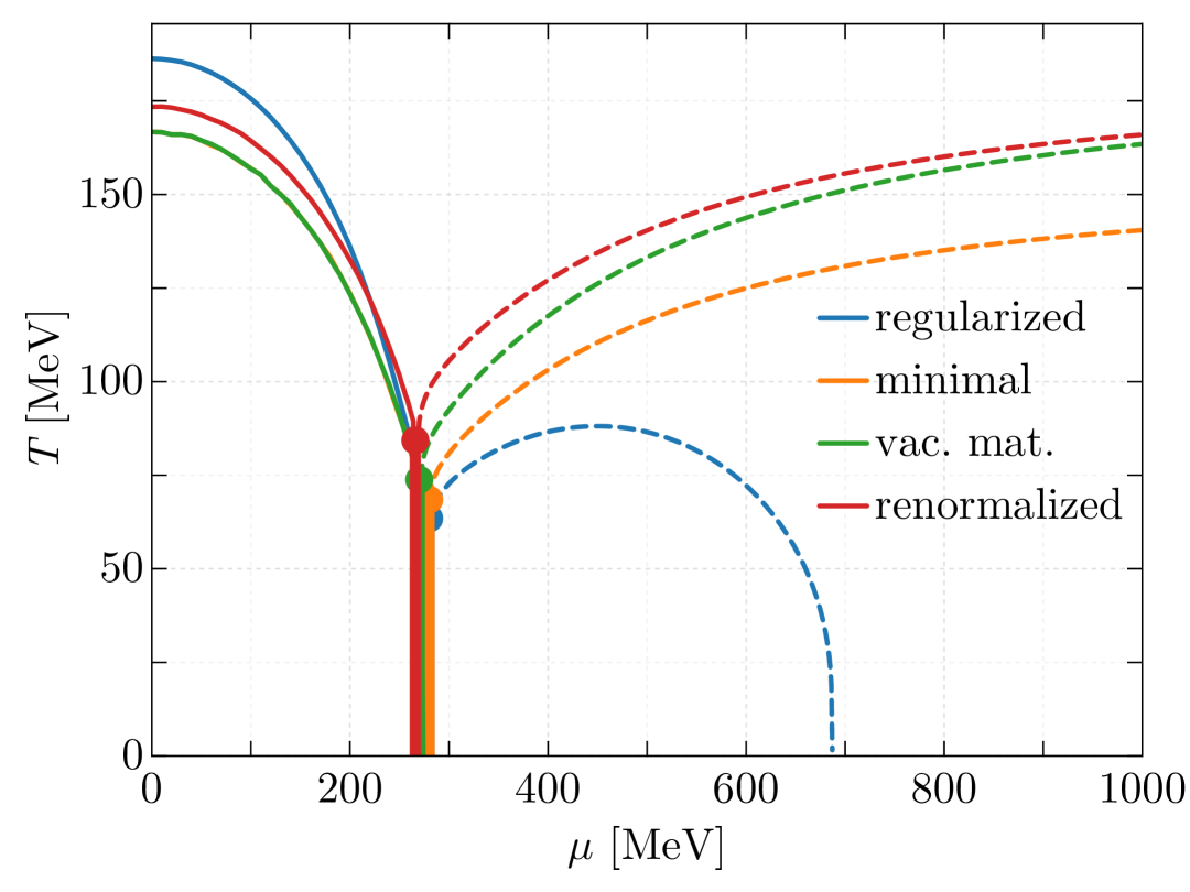
Figure 1: Phase diagram for the different approximations considered in this work. Thin solid lines indicate a crossover for the chiral condensate, thick lines indicate a first-order transition for both the chiral and diquark condensate, and dashed lines indicate a second-order transition for the diquark condensate. Critical endpoints are indicated as dots.

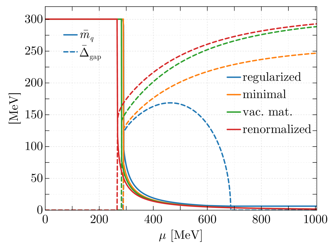
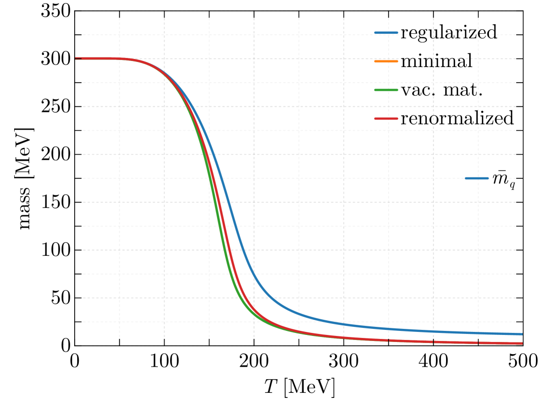
Figure 2: Quark mass $\bar{m}_{q}=g_{\phi}\bar{\sigma}$ and diquark gap $\bar{\Delta}_{\text{gap}}=g_{\Delta}\bar{\Delta}$ at $T=0\;\text{MeV}$ (left), and quark mass at $\mu=0$ (right) for the different approximations considered in this work. For $\mu=0$ (right) the diquark gap always vanishes, $\bar{\Delta}_{\text{gap}}=0$, and is not shown. Also note that for $\mu=0$ the two RGC schemes (minimal and vacuum matching) are identical.

In Fig. 1, we present the QMD phase diagram obtained within the regularized and renormalized mean‐field approximations, including both RGC schemes (vacuum matching and minimal). Thin solid lines denote the chiral crossover, defined by the minimum of $\ \partial_{\sigma}^{2}\Omega$ at fixed $\mu$, while thick solid lines indicate first‐order phase transitions in either the chiral or diquark sector. Dashed lines correspond to second‐order diquark transitions, and critical endpoints are marked by dots. All approximations share the same qualitative structure: at low $T$ and $\mu$, the system resides in a chirally broken phase without diquark pairing; at low $T$ and high $\mu$, it enters the chirally restored, color‐superconducting (2SC) phase; and at high $T$, chiral symmetry is restored with no diquark condensate. Quantitatively, however, significant differences emerge. In particular, the regMFA fails at large $\mu$: its diquark boundary bends downward and eventually disappears, reflecting the absence of high‐momentum contributions in the medium integrals. In contrast, both RGC schemes and the renormalized treatment maintain a 2SC phase up to arbitrarily large $\mu$. Moreover, the regMFA overestimates the chiral crossover temperature at low $\mu$, shifting the crossover line to higher $T$, and delaying the onset of the 2SC region to larger $\mu$ at low $T$.

To understand the origin of these differences, Fig. 2 shows the behavior of the condensates as functions of $\mu$ at $T=0$ (left panel) and of $T$ at $\mu=0$ (right panel). At zero temperature, the diquark gap $\bar{\Delta}_{\rm gap}$ in the regMFA initially increases but subsequently decreases and eventually vanishes. In contrast, the curves in the RGC schemes and the renormalized model exhibit the expected monotonic rise of $\bar{\Delta}_{\rm gap}$, followed by saturation to constant values as predicted by Eqs. 62 and 63. Similarly, the quark mass $\bar{m}_{q}=g_{\phi}\bar{\sigma}$ remains relatively large in the 2SC phase and tends toward a nonzero constant as $\mu\to\infty$ in the regMFA, while it vanishes in both RGC and renormalized schemes. These differences can be traced back to the limited integration domain in the regMFA, which suppresses diquark pairing and consequently delays the 2SC onset. A detailed analysis for this behavior is provided in Appendix D.

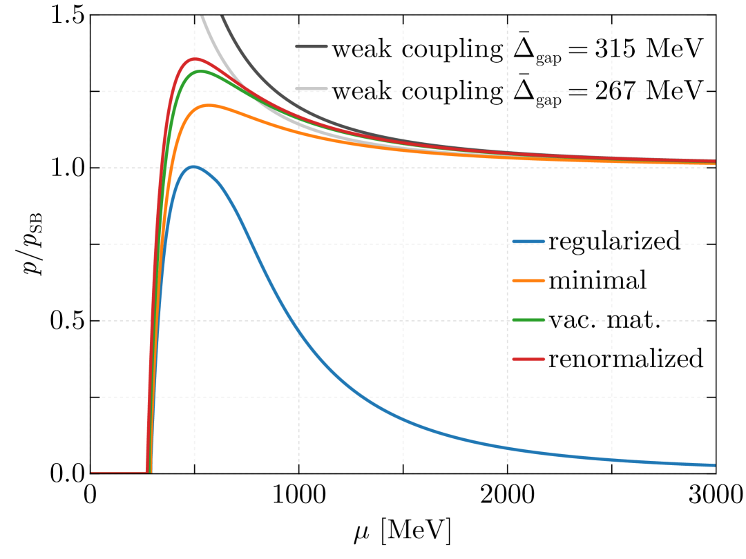
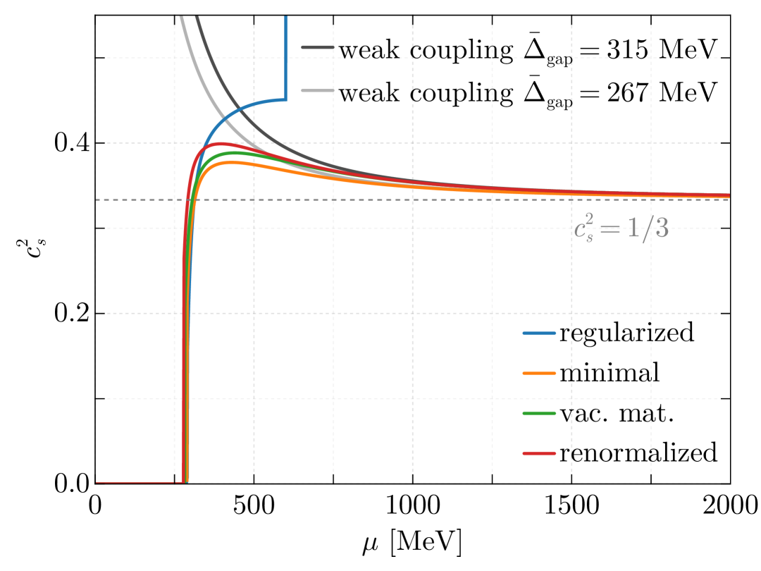
Figure 3: Pressure $p$ normalized to the Stefan-Boltzmann pressure $p_{\text{SB}}$ (left) and squared speed of sound (right) as functions of $\mu$ at $T=0\;\text{MeV}$. The black and gray solid lines indicate the asymptotic behavior of the pressure, Eq. 58, and of the speed of sound, Eq. 69, expected from a weak-coupling expansion. The gray dashed line marks the conformal limit, $c_{s}^{2}=1/3$ (right).

Similarly, at $\mu=0$, the regularized MFA restores chiral symmetry only at higher $T$, because the truncated thermal integrals slow down the decrease of $\bar{m}_{q}$ and leave it nonzero even as $T\to\infty$, similar to what happens at $T=0$ in the $\mu$ direction. In contrast, both the RGC and renormalized treatments drive $\bar{\sigma}\to 0$ at large $T$, giving a lower crossover temperature. Thus, in both the $\mu$- and $T$-directions, the limited integration domains in the regMFA favor chiral condensate persistence, shifting the chiral‐restoration crossover as well as the 2SC onset to higher external parameters when compared to the properly renormalized approaches.

The RGC vacuum matching and renormalized schemes differ only in their UV completion of the vacuum sector. Their small residual discrepancies arise from the choice of RG matching scale $\Lambda^{\prime}$ and the specific set of vacuum operators retained at that scale. Both approaches nevertheless agree closely with each other, showing that once vacuum matching is imposed, the detailed structure of the UV effective action has only a minor impact on the medium physics. The RGC minimal scheme, however, deviates further due to its different value of $\tilde{Z}_{\Delta}$, and accordingly its diquark gap approaches a different constant at large $\mu$: in the minimal RGC scheme one finds (see Eq. 63)

$$\lim_{\mu\to\infty}\bar{\Delta}^{(\mathrm{min})}_{\mathrm{gap}}=267.8\;\mathrm{MeV}\;,$$

whereas both the RGC vacuum matching and the renormalized schemes converge to (see Eq. 62)

$$\lim_{\mu\to\infty}\bar{\Delta}^{(\mathrm{vm})}_{\mathrm{gap}}=\lim_{\mu\to\infty}\bar{\Delta}^{(\mathrm{ren})}_{\mathrm{gap}}=315.2\;\mathrm{MeV}\;,$$

in agreement with the numerical results at $\mu=1000\;\text{MeV}$ in Fig. 2 (left).

Finally, as discussed in Section V.4, both the renormalized and RGC schemes exhibit BCS scaling for the critical temperature $T_{c}$ associated with the melting of the 2SC phase in the limit $\mu\rightarrow\infty$ as given by Eq. 73. Inserting the gaps at $\mu=1000\;\text{MeV}$, one finds

$$T_{c}^{\text{(min)}} \;\approx\;0.567\times 246.7\;\text{MeV}\;\approx 139.9\;\text{MeV}\;,$$

$$T_{c}^{\text{(vm)}}\;\approx\;T_{c}^{\text{(ren)}} \;\approx\;0.567\times 292.8\;\text{MeV}\;\approx 166.0\;\text{MeV}\;,$$

in agreement with the 2SC boundaries in Fig. 1 already at $\mu=1000$ MeV:

$$T_{c}^{(\text{min})} =140.5\;\text{MeV}\;,\quad\text{and}\quad$$

$$T_{c}^{(\text{ren})} =166.0\;\text{MeV}\;.$$

In Fig. 3, we show the pressure $p$ and the squared speed of sound $c_{s}^{2}$ at $T=0$ as functions of the chemical potential. As observed, the regMFA fails to approach the Stefan-Boltzmann limit for $\mu\to\infty$. Again, this deficiency is absent in the RGC and renormalized schemes, where the Stefan-Boltzmann limit is gradually attained in the high-density regime. For the speed of sound (right panel) we observe a peak exceeding the conformal limit $c_{s}^{2}=1/3$ , which is a characteristic feature of models incorporating diquark condensation [47, 48, 10, 11, 49]. As discussed in Section V.3, this quantity approaches the conformal value from above at large $\mu$, in contrast to expectations from perturbative QCD.

Additionally, in the regMFA the speed of sound exhibits an unphysical divergence at higher chemical potentials. This can be traced back to the behavior of the condensates in this approximation: as shown in Fig. 2, the diquark condensate vanishes and the chiral condensate $\bar{\sigma}$ tends toward a constant at large $\mu$. Under these conditions, the regulated medium integrals lead to a linear increase of the pressure $p$ with $\mu$, while the energy density $\epsilon$ asymptotically saturates to a constant value (see Appendix D for details). Since the squared speed of sound is defined as $c_{s}^{2}=\frac{dp}{d\epsilon},$ this leads to $\frac{dP}{d\epsilon}\to\infty\ ,$ implying a divergent $c_{s}^{2}$ at high chemical potentials in the regMFA.

We also compare the pressure and speed of sound to the weak coupling expansions Eq. 58 and Eq. 69, respectively, for two constant diquark gap values corresponding to the asymptotic values for the minimal and renormalized schemes. At large densities $\mu\gtrsim 1.5\;\text{GeV}$, we find a very good agreement between the weak coupling expansion and the numerical results as already noted in Ref. [20].

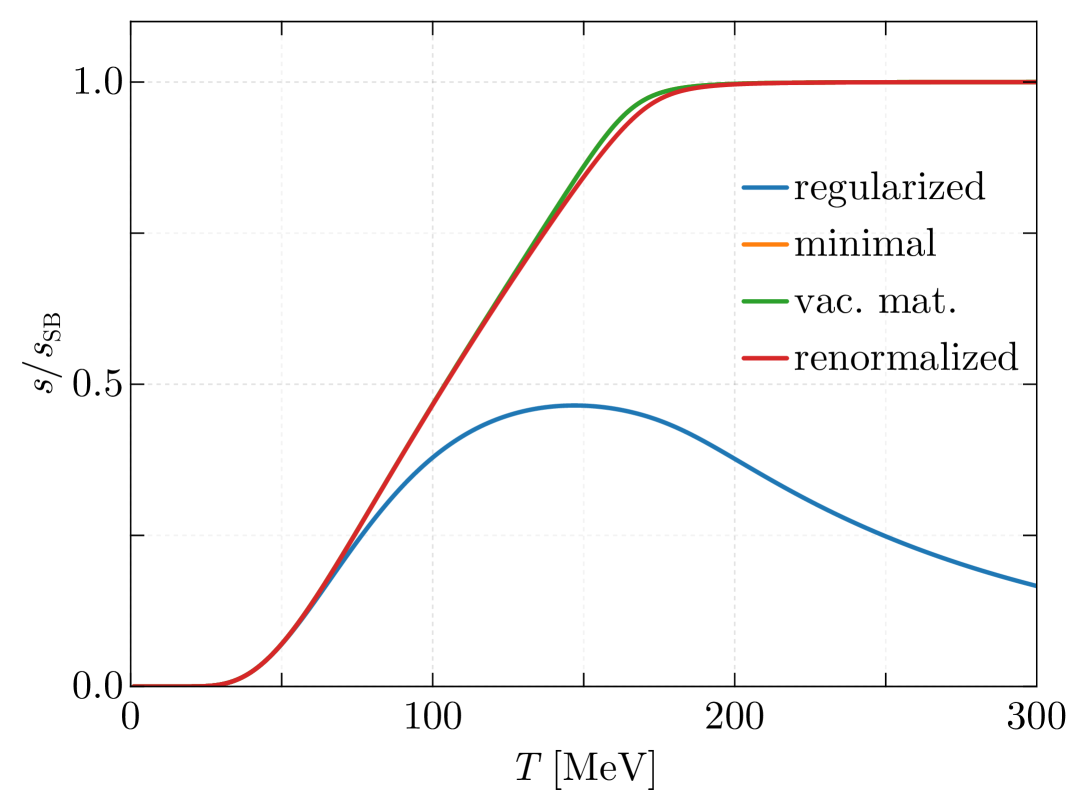
(a) $\mu=0\;\text{MeV}$

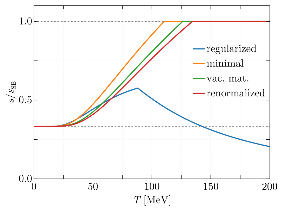
(b) $\mu=450\;\text{MeV}$

Figure 4: Entropy density $s$, normalized to the Stefan-Boltzmann entropy $s_{\text{SB}}$ (Eq. 81), as a function of $T$ at $\mu=0\;\text{MeV}$ (left) and $\mu=450\;\text{MeV}$ (right). The horizontal dashed lines indicate $s/s_{\text{SB}}=1$ and $s/s_{\text{SB}}=1/3$.

The same cutoff artifacts that distort the phase diagram and the speed of sound at higher values of $\mu$, are also visible in thermal observables. Because the regularized MFA omits high–momentum modes, its thermal pressure and entropy fall short of the Stefan–Boltzmann limits. Figure 4 compares the entropy density of the four approximations with the SB limit

$$s_{\mathrm{SB}}=\frac{N_{f}N_{c}}{3}\!\left(\frac{7\pi^{2}}{15}\,T^{3}\;+\;\mu^{2}T\right)\;.$$ (81)

For $\mu=0$ (left panel) no diquark condensate is present, and after the chiral crossover the quark mass drops to nearly zero. One therefore expects $s/s_{\mathrm{SB}}\!\to\!1$ at high temperature. Both RG-consistent curves and the renormalized curve meet this expectation, whereas the regMFA never reaches unity because the truncated momenta omit an increasing fraction of thermal modes as $T$ grows.

The right panel shows the same ratio at $\mu=450\;\text{MeV}$, where a 2SC condensate persists up to the critical temperature. Below $T_{c}$ the red–green quarks are gapped and exponentially suppressed, so only the ungapped blue quasi-quarks contribute; consequently $s/s_{\mathrm{SB}}\simeq 1/3$, a limit reached by all four approximations. Above $T_{c}$ the diquark gap vanishes and the quark mass is small; the RG-consistent and renormalized schemes therefore approach $s/s_{\mathrm{SB}}\!\to\!1$. The regularized MFA, however, breaks down once again, with the entropy ratio turning over and falling because the missing high-momentum thermal modes cannot be recovered by any further increase in $T$.

We emphasize that all thermodynamic observables tell the same story. Whether one probes along the temperature axis or along the chemical–potential axis, the truncated integrals in the regularized MFA restrict the available phase space and, as a consequence, distort chiral and superconducting transitions as well as bulk quantities such as the entropy. By contrast, the RG-consistent and renormalized calculations, which integrate over the full momentum range, consistently recover the Stefan–Boltzmann limits and preserve the expected pattern of phase transitions throughout the entire $(T,\mu)$ plane.

VI.3 Testing the BCS relation

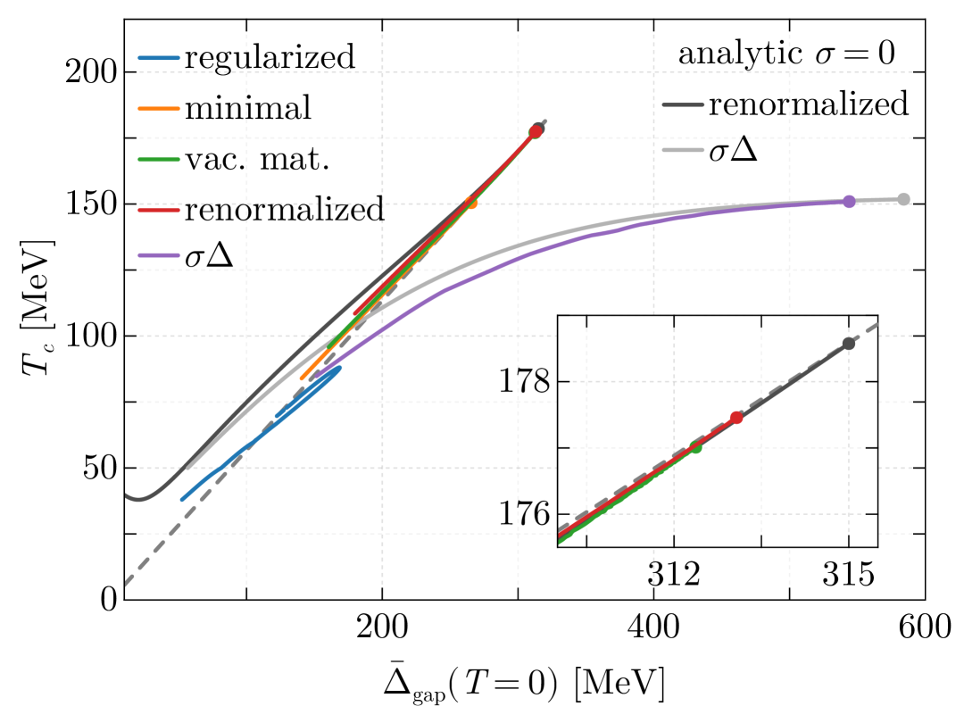
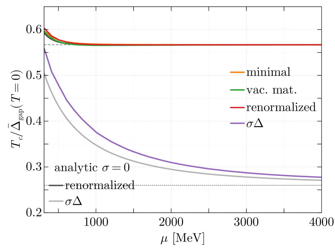
Figure 5: Left: Critical temperature $T_{c}$ versus the diquark gap $\bar{\Delta}_{\text{gap}}$ at $T=0$. The gray solid dots indicate the value reached for asymptotically large chemical potential Eqs. 62 and 63. Colored solid dots are obtained numerically at $\mu=4\;\text{GeV}$. The dashed gray line indicates the BCS scaling relation $T_{c}\propto 0.567\bar{\Delta}_{\text{gap}}$. Right: Ratio $T_{c}/\bar{\Delta}_{\text{gap}}(T=0)$ as a function of the chemical potential $\mu$. The dashed gray line indicates the BCS scaling $T_{c}\propto 0.567\bar{\Delta}_{\text{gap}}$, while the dotted line shows $T_{c}\propto 0.260\bar{\Delta}_{\text{gap}}$, which corresponds to the asymptotic value in the $\sigma\Delta$ scheme for this chosen set of parameters.

With $\bar{\Delta}(T=0)$ and $T_{c}$ at our hands we can compare their ratio with the BCS result and also with the numerical results obtained outside of the chiral limit. The results are shown in Fig. 5, where in the left panel $T_{c}$ is plotted as a function $\bar{\Delta}_{\text{gap}}(T=0)$, and in the right panel their ratio against $\mu$.

First we note that the BCS relation is valid at $\mu\to\infty$, see Eq. 73. At finite chemical potential the exact results deviate slightly. This is to be expected as the BCS relation is strictly valid only in the small coupling limit $\bar{\Delta}_{\text{gap},0}^{2}/\mu^{2}\to 0$, which —when solving the gap equation for $\bar{\Delta}$ consistently—can only be achieved at asymptotically large $\mu$ values. However, Fig. 5 shows that the BCS relation remains a good approximation even at lower $\mu$ values. Note that for the regularized model, we only show points where $\bar{\Delta}_{\text{gap}}>50\;\text{MeV}$ to avoid most of the unphysical region where $\bar{\Delta}_{\text{gap}}$ decreases as $\mu$ increases (see Fig. 2). In the renormalized, RGC–minimal, and RGC–vacuum–matching schemes the linear BCS scaling is manifest at large chemical potential, where the quark mass vanishes, and all three curves satisfy the BCS relation Eq. 73. Specifically, the analytical result obtained in Eq. 72 for the renormalized model in the chiral limit aligns well with the behavior observed in Figs. 5 and 5 at higher $\bar{\Delta}$ and $\mu$ values. By contrast, the scaling behaviour in the $\sigma\Delta$ scheme is qualitatively different. As discussed in Section V.4, this scheme yields a different asymptotic value for the diquark gap, yet, consistent with Eq. 74, the critical temperature approaches the same limit as in the minimal scheme. This distinction is clearly visible in the left panel of Fig. 5. Therefore among the RGC schemes discussed in this paper, only the $\sigma\Delta$ scheme fails to follow the BCS relation.

We conclude that although both the $\sigma\Delta$ and the vacuum matching schemes employ the same set of vacuum parameters, the excessive and unnecessary subtractions in the $\sigma\Delta$ scheme leads to distinct thermodynamic behavior. As noted in Ref. [17], such unnecessary subtractions in RGC schemes can yield unexpected consequences that are not anticipated from a physical standpoint. The discrepancy observed here regarding the BCS relation is of the same nature; the excessive subtraction in all $\Delta$-dependent RGC schemes (including schemes used in Ref. [20] and mass-dependent and massless schemes in Ref. [17]) results in a deviation from the expected BCS relation.

It is also worth noting that the extent to which the BCS relation is realized and how the asymptotic limit is approached are sensitive to the choice of parameters. With different parameter choices, the BCS relation might become a good approximation only at substantially larger values of $\mu$. Thus, the linear scaling along a large range of $\bar{\Delta}_{\text{gap}}$ values observed in Figs. 5 and 5 (left) may be coincidental.

VII Summary, Discussions and Conclusions

In this work, we have presented a systematic comparison between two conceptually distinct yet complementary approaches to rendering the two–flavor Quark–Meson–Diquark (QMD) model ultraviolet safe: a renormalized formulation and an RG–consistent mean–field treatment that incorporates ideas from the functional renormalization-group (FRG). After fixing all couplings through a common set of vacuum parameters, both frameworks reproduce the same low–energy phenomenology by construction and, perhaps more importantly, yield the same qualitative — and to a large extent even quantitative — description of dense, cold quark matter. They generate identical phase structures, approach the Stefan–Boltzmann limit at large chemical potential, respect the BCS relation $T_{\mathrm{c}}=e^{\gamma}\Delta_{0}/\pi$ in the chiral limit and avoid the notorious cutoff artifacts that affect naïvely regularized mean–field calculations.

Our analysis reveals that the regularized mean-field approximation with explicit diquark degrees of freedom exhibits unphysical thermodynamics at high densities and temperatures. Notably, the pressure grows only linearly with $\mu$, the Stefan–Boltzmann limit is never satisfied, and the speed of sound diverges, signaling a breakdown of the approximation. Since many earlier hybrid-star studies rely on regMFA diquark equations of state at these densities, they may inevitably inherit such inconsistencies, potentially leading to erroneous conclusions about stellar properties. Therefore, a properly renormalized or RG-consistent treatment is essential for making robust astrophysical predictions.

Taken together, our findings demonstrate that the QMD model can serve as a more robust framework for describing color-superconducting matter, provided that either renormalization or RG consistency is imposed.

The two approaches nevertheless differ in important details. In the renormalized model, all vacuum and medium divergences are absorbed into scale–dependent bare couplings, rendering the effective action exactly independent of the regulator. The price for this regulator independence is an enlarged parameter space: additional couplings proportional to $\phi^{2}|\Delta|^{2}$, $|\Delta|^{4}$ and via the diquark wave-function renormalization to $\mu^{2}|\Delta|^{2}$ must be allowed to run with the cutoff. By contrast, RG-consistent mean-field schemes keep the microscopic action fixed, but compensate for the residual cutoff dependence by enforcing RG consistency via appropriate matching conditions.

Although an RG–consistent (RGC) mean-field construction ensures that physical observables become independent of the ultraviolet cutoff, i.e., in the limit $\Lambda\to\infty$, it does not uniquely prescribe how to eliminate medium–induced divergences. The corresponding counterterms are therefore scheme-dependent, and different prescriptions can alter finite-density observables even after the vacuum parameters have been fixed. In Ref. [17], it was shown how these schemes can be related to the wave-function renormalization of the diquark field, $Z_{\Delta}$. Motivated by this insight, we introduced a vacuum-matching RGC scheme in which $Z_{\Delta}$ is fixed in the vacuum to a value in principle accessible via first-principle QCD calculations.

With this choice, the in-medium flow reproduces the diquark gap obtained in the fully renormalized QMD model up to sub-leading $1/\mu^{2}$ corrections, while preserving the cutoff independence characteristic of all RGC constructions. In this sense, the vacuum-matching scheme retains the conceptual clarity of the prescription in Ref. [20] and the minimal prescription in Ref. [17]. By anchoring the construction to a physical vacuum observable, it largely eliminates the residual scheme ambiguity that would otherwise persist among RGC implementations.

A final crisp benchmark is the BCS relation, $T_{c}=e^{\gamma}\bar{\Delta}_{\text{gap}}(T=0)/\pi$. We find that this ratio is exactly reproduced in the $\mu\to\infty$ limit by the renormalized QMD model and by RG-consistent schemes whose medium subtraction can be reinterpreted as a diquark wave-function renormalization, specifically, the minimal and vacuum-matching variants. In contrast, schemes in which the subtraction acquires an additional $\Delta$-dependent structure (such as the $\sigma\Delta$ scheme of Ref. [20]) violate the BCS ratio. This underscores, once again, that seemingly innocuous choices for removing medium divergences can significantly alter key in-medium observables. We emphasize, however, that this should not be taken as a criterion for discarding specific RG-consistent schemes. Rather, it highlights the intrinsic scheme dependence in the subtraction of medium divergences, an ambiguity that persists even after matching to vacuum parameters.

Our analytic solution of the $T=0$ gap equation reveals that, in the limit $\mu\to\infty$, the diquark gap approaches a finite constant — see Eqs. 62 and 63. Remarkably, in both the renormalized model and RGC vacuum-matching scheme, this asymptotic value depends only on the vacuum quark mass, the diquark Yukawa coupling, and the vacuum wave-function renormalization of the diquark field, with every explicit trace of the UV regulator eliminated. Renormalization and RG consistency thus remove the cutoff from the formalism without severing the link between vacuum physics and dense-matter observables: once the vacuum parameters are fixed, the entire finite-$T$ / finite-$\mu$ sector of the QMD model becomes a genuine prediction of mean-field dynamics.

The most compelling next step is therefore to determine these correlators directly from QCD — e.g., via lattice calculations or by matching continuum FRG/DSE computation. Such an ab-initio calibration would turn the model into a parameter-free tool for mapping the phase structure and the equation of state of dense matter. This procedure would offer a decisive test of whether a mean‑field QMD model, once anchored to realistic vacuum observables, can simultaneously satisfy astrophysical constraints at least without requiring the inclusion of beyond‑mean‑field fluctuations.

With the vacuum parameter fixing provided by first-principles QCD in place, several phenomenologically important extensions become both natural and reliable. The present two‑flavor framework can, for instance, be generalized to the three‑flavor case. In Ref. [17], the melting pattern of the color–flavor‑locked (CFL) phase was analyzed within an RG‑consistent NJL framework. The results reproduce earlier Ginzburg–Landau predictions [50], whereas the conventional cutoff‑regularized NJL model fails to do so. It would be instructive to extend this analysis to a three-flavor QMD model.

For astrophysical applications, a repulsive vector interaction, together with electric-charge, isospin and color-neutrality constraints, must be incorporated to obtain an equation of state compatible with $\sim 2\,M_{\odot}$ neutron stars and their tidal-deformability bounds [51, 52, 53, 54, 49]. In addition, the regulator-independent framework developed here provides a clean setting to revisit spatially modulated chiral or pairing phases, whose very existence crucially depends on careful control of cutoff artifacts [55, 56, 57]. Work along these lines is ongoing and will be reported elsewhere.

To conclude, we have demonstrated that both renormalization and RG consistency eliminate the regulator ambiguities inherent in the QMD model, yielding mutually consistent and analytically tractable descriptions of dense quark matter. Together, these approaches provide a powerful and flexible framework for future studies aimed at connecting microscopic QCD dynamics with astrophysical observations of compact stars.

Data Availability

The numerical data presented in all figures in this work are openly available in the ancillary files of the corresponding arXiv submission.

Appendix A Derivation of the renormalized potential

Fixing $\tilde{f}_{\pi}$, the remaining vacuum parameters in Table 1 are found by evaluating derivatives of the effective potential Eq. 3 in vacuum, which yields

$$\tilde{m}_{\sigma}^{2}= m_{\phi}^{2}(\Lambda)+3\lambda_{\phi}(\Lambda){\tilde{f}_{\pi}}^{2}+\left.\left(\partial_{\sigma}^{2}L_{\Lambda}\right)\right|_{\text{vac}}\;,$$ (82)

$$\tilde{m}_{\Delta}^{2}= m_{\Delta}^{2}(\Lambda)+\frac{1}{2}\lambda_{\text{mix}}(\Lambda){\tilde{f}_{\pi}}^{2}+\frac{1}{2}\left.\left(\partial_{\Delta}^{2}L_{\Lambda}\right)\right|_{\text{vac}}\;,$$ (83)

$$\tilde{\lambda}_{\text{mix}}= \lambda_{\text{mix}}(\Lambda)+\frac{1}{2}\left.\left(\partial_{\sigma}^{2}\partial_{\Delta}^{2}L_{\Lambda}\right)\right|_{\text{vac}}\;,$$ (84)

$$\tilde{\lambda}_{\Delta}= \lambda_{\Delta}(\Lambda)+\frac{1}{24}\left.\left(\partial_{\Delta}^{4}L_{\Lambda}\right)\right|_{\text{vac}}\;,$$ (85)

$$\tilde{Z}_{\Delta}= Z_{\Delta}(\Lambda)-\frac{1}{16}\left.\left(\partial_{\mu}^{2}\partial_{\Delta}^{2}L_{\Lambda}\right)\right|_{\text{vac}}\;.$$ (86)

Eq. 20 and Eqs. 82 to 86 form a simple linear system of equations that can be solved for an expression of the 6 UV scale dependent bare parameters in terms of the correlators. The solution of this linear system yields

$$m_{\phi}^{2}(\Lambda)=-\frac{1}{2{\tilde{f}_{\pi}}}\Big{\{}\tilde{m}_{\sigma}^{2}{\tilde{f}_{\pi}}-3c-{\tilde{f}_{\pi}}\left.\left(\partial_{\sigma}^{2}L_{\Lambda}\right)\right|_{\text{vac}}+3\left.\left(\partial_{\sigma}L_{\Lambda}\right)\right|_{\text{vac}}\Big{\}}\;,$$ (87)

$$m_{\Delta}^{2}(\Lambda)=\tilde{m}_{\Delta}^{2}-\frac{1}{2}\tilde{\lambda}_{\text{mix}}{\tilde{f}_{\pi}}^{2}-\frac{1}{2}\left.\left(\partial_{\Delta}^{2}L_{\Lambda}\right)\right|_{\text{vac}}+\frac{{\tilde{f}_{\pi}}^{2}}{4}\left.\left(\partial_{\sigma}^{2}\partial_{\Delta}^{2}L_{\Lambda}\right)\right|_{\text{vac}}\;,$$ (88)

$$\lambda_{\phi}(\Lambda)=\frac{1}{2{\tilde{f}_{\pi}}^{3}}\Big{\{}\tilde{m}_{\sigma}^{2}{\tilde{f}_{\pi}}-c-\tilde{f}_{\pi}\left.\left(\partial_{\sigma}^{2}L_{\Lambda}\right)\right|_{\text{vac}}+\left.\left(\partial_{\sigma}L_{\Lambda}\right)\right|_{\text{vac}}\Big{\}}\;,$$ (89)

$$\lambda_{\text{mix}}(\Lambda)=\tilde{\lambda}_{\text{mix}}-\frac{1}{2}\left.\left(\partial_{\sigma}^{2}\partial_{\Delta}^{2}L_{\Lambda}\right)\right|_{\text{vac}}\;,$$ (90)

$$\lambda_{\Delta}(\Lambda)=\tilde{\lambda}_{\Delta}-\frac{1}{24}\left.\left(\partial_{\Delta}^{4}L_{\Lambda}\right)\right|_{\text{vac}}\;,$$ (91)

$$Z_{\Delta}(\Lambda)=\tilde{Z}_{\Delta}+\frac{1}{16}\left.\left(\partial_{\mu}^{2}\partial_{\Delta}^{2}L_{\Lambda}\right)\right|_{\text{vac}}\;.$$ (92)

Using the expression for the loop contribution Eq. 4, we can write the bare parameters as

$$m_{\phi}^{2}(\Lambda)=-\frac{1}{2}\tilde{m}_{\sigma}^{2}+\frac{3c}{2\tilde{f}_{\pi}}+2N_{f}\int_{|\vec{p}|<\Lambda}\frac{3g_{\phi}^{2}}{2\epsilon_{q,\text{vac}}^{3}}\left(2p^{2}+3m_{q,\text{vac}}^{2}\right)\;,$$ (93)

$$m_{\Delta}^{2}(\Lambda)=\tilde{m}_{\Delta}^{2}-\frac{1}{2}\tilde{\lambda}_{\text{mix}}{\tilde{f}_{\pi}}^{2}+2N_{f}\int_{|\vec{p}|<\Lambda}\frac{g_{\Delta}^{2}p^{2}}{2\epsilon_{q,\text{vac}}^{5}}\left(2p^{2}+5m_{q,\text{vac}}^{2}\right)\;,$$ (94)

$$\lambda_{\phi}(\Lambda)=\frac{1}{2{\tilde{f}_{\pi}}^{2}}\tilde{m}_{\sigma}^{2}-\frac{c}{2{\tilde{f}_{\pi}}^{3}}-2N_{f}\int_{|\vec{p}|<\Lambda}\frac{3g_{\phi}^{4}}{2\epsilon_{q,\text{vac}}^{3}}\;,$$ (95)

$$\lambda_{\text{mix}}(\Lambda)=\tilde{\lambda}_{\text{mix}}-2N_{f}\int_{|\vec{p}|<\Lambda}\frac{g_{\Delta}^{2}g_{\phi}^{2}}{\epsilon_{q,\text{vac}}^{5}}\left(p^{2}-2m_{q,\text{vac}}^{2}\right)\;,$$ (96)

$$\lambda_{\Delta}(\Lambda)=\tilde{\lambda}_{\Delta}-2N_{f}\int_{|\vec{p}|<\Lambda}\frac{g_{\Delta}^{4}}{4\epsilon_{q,\text{vac}}^{3}}\;,$$ (97)

$$Z_{\Delta}(\Lambda)=\tilde{Z}_{\Delta}-2N_{f}\int_{|\vec{p}|<\Lambda}\frac{g_{\Delta}^{2}}{4\epsilon_{q,\text{vac}}^{3}}\;,$$ (98)

where we introduced $m_{q,\text{vac}}=g_{\phi}\tilde{f}_{\pi}$ and $\epsilon_{q,\text{vac}}=\sqrt{p^{2}+m_{q,\text{vac}}^{2}}$. Finally, we obtain the renormalized and UV scale independent potential by sending $\Lambda\to\infty$ in the momentum integration of the effective potential, which results in Section III.2.

Appendix B $\beta$-functions of the model couplings

From the mean-field flow Eq. 33, we can evaluate the $\beta$-functions of the relevant couplings of the model. At vanishing temperature and for the sharp regulator, the mean-field flow reduces to

$$\partial_{k}\Omega_{k}=\frac{N_{f}k^{2}}{\pi^{2}}\bigg{\{}\epsilon_{q}(k)+E_{q}^{-}(k)+E_{q}^{+}(k)-\epsilon_{q}^{-}(k)\theta\left(\epsilon_{q}^{-}(k)\right)\bigg{\}}\;.$$ (99)

In the following, we neglect the last term $-\epsilon_{q}^{-}(k)\theta\left(\epsilon_{q}^{-}(k)\right)$ arising from the thermal part of the potential, as it yields an irrelevant contribution in the limit $k\to\infty$. We then perform a Taylor expansion of the effective potential

$$\Omega_{k}=\frac{1}{2}m^{2}_{\phi,k}\phi^{2}+\frac{1}{4}\lambda_{\phi,k}\sigma^{4}+\frac{1}{2}\lambda_{\text{mix},k}\sigma^{2}\Delta^{2}+m^{2}_{\Delta,k}\Delta^{2}+\lambda_{\Delta,k}\Delta^{4}-4Z_{\Delta,k}\mu^{2}\Delta^{2}+\cdots\;,$$ (100)

and insert this expansion in the mean-field flow Eq. 99. The $\beta$-functions of the couplings are obtained by comparing coefficients, yielding

$$\partial_{k}m^{2}_{\phi,k}=\frac{6g_{\phi}^{2}}{\pi^{2}}k\;,\quad\partial_{k}\lambda_{\phi,k}=-\frac{3g_{\phi}^{4}}{\pi^{2}}\frac{1}{k}\;,\quad\partial_{k}m^{2}_{\Delta,k}=\frac{2g_{\Delta}^{2}}{\pi^{2}}k\;,\quad$$ (101)

$$\partial_{k}\lambda_{\Delta,k}=-\frac{g_{\Delta}^{4}}{2\pi^{2}}\frac{1}{k}\;,\quad\partial_{k}\lambda_{\text{mix},k}=-\frac{2g_{\Delta}^{2}g_{\phi}^{2}}{\pi^{2}}\frac{1}{k}\;,\quad\partial_{k}Z_{\Delta,k}=-\frac{g_{\Delta}^{2}}{2\pi^{2}}\frac{1}{k}\;.$$

This directly leads to the following solutions for the scale dependence of the couplings:

$$m^{2}_{\phi,k} =\frac{3g_{\phi}^{2}}{\pi^{2}}(k^{2}-{k_{0}}^{2})+m^{2}_{\phi,k_{0}}\;,$$ (102)

$$\lambda_{\phi,k} =-\frac{3g_{\phi}^{4}}{\pi^{2}}\ln\frac{k}{k_{0}}+\lambda_{\phi,k_{0}}\;,$$ (103)

$$m^{2}_{\Delta,k} =\frac{g_{\Delta}^{2}}{\pi^{2}}(k^{2}-{k_{0}}^{2})+m^{2}_{\Delta,k_{0}}\;,$$ (104)

$$\lambda_{\Delta,k} =-\frac{g_{\Delta}^{4}}{2\pi^{2}}\ln\frac{k}{k_{0}}+\lambda_{\Delta,k_{0}}\;,$$ (105)

$$\lambda_{\text{mix},k} =-\frac{2g_{\Delta}^{2}g_{\phi}^{2}}{\pi^{2}}\ln\frac{k}{k_{0}}+\lambda_{\text{mix},k_{0}}\;,$$ (106)

$$Z_{\Delta,k} =-\frac{g_{\Delta}^{2}}{2\pi^{2}}\ln\frac{k}{k_{0}}+Z_{\Delta,k_{0}}\;.$$ (107)

Here, $k_{0}$ represents an arbitrary reference scale. Notably, if we choose $k=\Lambda$, the RG scale dependence of the couplings exactly matches the $\Lambda$-dependence of the renormalized model couplings, as given in Eqs. 11 to 16. This explicitly demonstrates that, as expected, the RG-consistency generates the appropriate counterterms introduced in the renormalized model.

Appendix C BCS analysis at $T_{c}$

Subtraction of the gap equations in Eq. 70 yields the relation

$$\begin{split}&\left.\frac{\partial\Omega^{\text{eff}}_{\text{ren}}(\sigma,\Delta;T_{c},\mu)}{\partial\Delta}\right|_{\begin{subarray}{c}\sigma=0\\ \Delta=0\end{subarray}}-\left.\frac{\partial\Omega^{\text{eff}}_{\text{ren}}(\sigma,\Delta;0,\mu)}{\partial\Delta}\right|_{\begin{subarray}{c}\sigma=0\\ \Delta=\bar{\Delta}_{0}\end{subarray}}=4\tilde{\lambda}_{\Delta}\Delta_{0}^{2}\\ &\quad-g_{\Delta}^{2}2N_{f}\int_{\vec{p}}\left\{\frac{1}{E_{q,0}^{-}}+\frac{1}{E_{q,0}^{+}}+\frac{\Delta_{\text{gap},0}^{2}}{\epsilon_{q,\text{vac}}^{3}}-\frac{1}{\epsilon_{q}^{-}}\tanh\frac{\epsilon_{q}^{-}}{2T_{c}}-\frac{1}{\epsilon_{q}^{+}}\tanh\frac{\epsilon_{q}^{+}}{2T_{c}}\right\}\;,\end{split}$$ (108)

where, assuming a vanishing chiral condensate, we have

$$E_{q,0}^{\pm}\;=\;\sqrt{(\epsilon_{q}^{\pm})^{2}+\Delta_{0}^{2}}\;,\qquad\epsilon_{q}^{\pm}\;=\;p\pm\mu\;,$$

with $p=|\vec{p}|$. Since both gap equations vanish, their difference also vanishes. The resulting condition implicitly defines the location of the second-order phase boundary of the 2SC phase at a given chemical potential $\mu$, via the corresponding zero-temperature gap $\Delta_{0}(\mu)\equiv\Delta(T=0,\mu)$. Solving this condition for $T$ yields the critical temperature $T_{c}$.

To proceed, we split the remaining momentum integral into two convergent parts, one for each $\tanh$ term. Because each part converges separately, we can shift and unify the integration limits. Rewriting LABEL:app:bcssubtr in this way, we obtain

$$0={} 4\tilde{\lambda}_{\Delta}\Delta_{0}^{2}-g_{\Delta}^{2}2N_{f}\left\{\int_{\vec{p}}\bigg{(}\frac{1}{2}\frac{\Delta_{\text{gap},0}^{2}}{\epsilon_{q,\text{vac}}^{3}}+\frac{1}{E_{q,0}^{-}}-\frac{1}{\epsilon_{q}^{-}}\tanh\frac{\epsilon_{q}^{-}}{2T_{c}}\bigg{)}+\int_{\vec{p}}\bigg{(}\frac{1}{2}\frac{\Delta_{\text{gap},0}^{2}}{\epsilon_{q,\text{vac}}^{3}}+\frac{1}{E_{q,0}^{+}}-\frac{1}{\epsilon_{q}^{+}}\tanh\frac{\epsilon_{q}^{+}}{2T_{c}}\bigg{)}\right\}\;,$$ (109)

By shifting the integration variable in the first integral, $p\to p-\mu$, and in the second integral, $p\to p+\mu$, and then separating the even and odd parts of the integrand, the two integrals can be combined into a single one,

$$\begin{split}0={}&4\tilde{\lambda}_{\Delta}\Delta_{0}^{2}-g_{\Delta}^{2}2N_{f}\int_{\vec{p}}\bigg{\{}\frac{\Delta_{\text{gap},0}^{2}\,(p-\mu)^{2}}{2\left((p-\mu)^{2}+m_{q,\text{vac}}^{2}\right)^{3/2}}+\frac{\Delta_{\text{gap},0}^{2}\,(p+\mu)^{2}}{2\left((p+\mu)^{2}+m_{q,\text{vac}}^{2}\right)^{3/2}}\\ &+\frac{(p-\mu)^{2}}{\sqrt{p^{2}+\Delta_{\text{gap},0}^{2}}}+\frac{(p+\mu)^{2}}{\sqrt{p^{2}+\Delta_{\text{gap},0}^{2}}}-2(p^{2}+\mu^{2})\frac{1}{p}\tanh\frac{p}{2T_{c}}\bigg{\}}\;.\end{split}$$ (110)

The integral can be evaluated analytically by inserting the series representation

$$\tanh x\;=\;2\,\sinh x\sum_{k=1}^{\infty}(-1)^{\,k+1}e^{\,(1-2k)x}\;.$$ (111)

For all $k\geq 2$ the resulting terms can be resummed into the infinite product

$$\prod_{k=1}^{\infty}\!\Bigl{(}1-\frac{1}{4k^{2}}\Bigr{)}\;=\;\frac{2}{\pi}\;,$$ (112)

while the remaining contribution from the $k=1$ term is obtained by an integral,

$$\int_{0}^{\infty}dx\left\{-\frac{1}{1+x}+\frac{2}{x}e^{-x}\sinh(x)\right\}=\ln 2+\gamma\;,$$ (113)

where $\gamma\simeq 0.5772$ is the Euler–Mascheroni constant. Summing all contributions for the integral in Eq. 110, this whole expression can be evaluated as

$$0=4\tilde{\lambda}_{\Delta}\Delta_{0}^{2}-\frac{g_{\Delta}^{2}}{{3\pi^{2}}}\left\{2\pi^{2}T_{c}^{2}+12\mu^{2}\Big{(}\ln\frac{\pi T_{c}}{\Delta_{\text{gap},0}}-\gamma\Big{)}+3\Delta_{\text{gap},0}^{2}\Big{(}2\ln\frac{\Delta_{\text{gap},0}}{m_{q,\text{vac}}}-1\Big{)}\right\}\;.$$ (114)

The expression above can be re-written as

$$\Big{(}\frac{\pi^{2}}{3\,\mu^{2}}T_{c}^{2}\Big{)}\;\exp{\Big{(}\frac{\pi^{2}}{3\,\mu^{2}}T_{c}^{2}\Big{)}}=\frac{\Delta_{\text{gap},0}^{2}}{3\mu^{2}}\,\exp\!\Biggl{[}2\gamma+\frac{\Delta_{\text{gap},0}^{2}}{\mu^{2}}\Biggl{(}\frac{1}{2}+\frac{2\pi^{2}}{g_{\Delta}^{4}}\tilde{\lambda}_{\Delta}-\ln\!\frac{\Delta_{\text{gap},0}}{m_{q,\text{vac}}}\Biggr{)}\Biggr{]}\;.$$ (115)

Now, starting from the transcendental equation

$$z\,e^{z}=C\;,$$ (116)

one introduces the (multi-valued) Lambert W-function [58], defined implicitly by

$$W(x)\,e^{W(x)}\;=\;x\;.$$ (117)

Applying this definition to Eq. 116 gives the formal solution

$$z\;=\;W(C)\;.$$ (118)

Employing Eq. 118, the critical temperature $T_{c}$ in Eq. 115 can be written compactly as

$$T_{c}^{2}(\Delta_{0},\mu)=\frac{3\mu^{2}}{\pi^{2}}\,W\!\Biggl{(}\frac{\Delta_{\text{gap},0}^{2}}{3\mu^{2}}\,\exp\!\Biggl{[}2\gamma+\frac{\Delta_{\text{gap},0}^{2}}{\mu^{2}}\Biggl{(}\frac{1}{2}+\frac{2\pi^{2}}{g_{\Delta}^{4}}\tilde{\lambda}_{\Delta}-\ln\!\frac{\Delta_{\text{gap},0}}{m_{q,\text{vac}}}\Biggr{)}\Biggr{]}\Biggr{)}\;,$$ (119)

where the branch of the $W$-function must be chosen such that the second root is positive and the resulting $T_{c}$ is real and positive.

Appendix D Behavior of regMFA at high chemical potential

In the regularized QMD model, as seen in Fig. 2, the diquark condensate vanishes at sufficiently large chemical potentials, leaving only a finite constituent–quark mass which remains at a constant value. This behavior can be understood analytically as follows. For chemical potentials satisfying $\mu>\sqrt{\Lambda^{2}+m_{q}^{2}}$ , the loop contribution to the effective potential Eq. 4 at $T=0$ reads

$$L_{\Lambda}\!\bigl{(}\sigma,\Delta;T=0\bigr{)}\;=\;-2N_{f}\!\int_{|\vec{p}|<\Lambda}\!\Bigl{\{}\,E_{q}^{+}+E_{q}^{-}+\frac{1}{2}\epsilon_{q}^{+}+\frac{1}{2}|\epsilon_{q}^{-}|\;\Bigr{\}}\;.$$ (120)

Expanding this expression in powers of $\Delta/\Lambda$ gives

$$L_{\Lambda}(\sigma,\Delta;T=0)\;=\;-\,\frac{N_{f}\,\Lambda^{3}}{\pi^{2}}\mu+\frac{N_{f}\,\,g_{\Delta}^{2}\,\Delta^{2}}{\pi^{2}}\mu\,\Lambda\Biggl{[}1-\frac{\sqrt{{\mu^{2}-m_{q}^{2}}}}{\Lambda}\,\operatorname{arctanh}\!\frac{\Lambda}{\sqrt{\mu^{2}-m_{q}^{2}}}+\mathcal{O}\!\bigl{(}\Delta^{2}/\Lambda^{2}\bigr{)}\Biggr{]}\;.$$ (121)

Inserting this into the effective potential together with the bosonic potential Eq. 75 (with $Z_{\Delta}=0$) and differentiating with respect to $\Delta$ to get the gap equation yields

$$\frac{\partial\Omega_{\text{reg}}^{\text{eff}}(\sigma,\Delta;T=0)}{\partial\Delta}\;=\;\Delta\,\Biggl{\{}2m_{\Delta}^{2}\;+\;\frac{2N_{f}g_{\Delta}^{2}}{\pi^{2}}\,\mu\,\Lambda\Biggl{[}1\;-\;\frac{\sqrt{{\mu^{2}-m_{q}^{2}}}}{\Lambda}\,\operatorname{arctanh}\!\frac{\Lambda}{\sqrt{\mu^{2}-m_{q}^{2}}}+\;\mathcal{O}\!\bigl{(}\Delta^{2}/\Lambda^{2}\bigr{)}\Biggr{]}\Biggr{\}}=0\;.$$ (122)

Thus $\bar{\Delta}=0$ (and $g_{\phi}\bar{\sigma}=\bar{m}_{q}$) is a non-trivial solution provided the bracket vanishes. Defining $\mu_{c}$ by that condition,

$$2m_{\Delta}^{2}\;+\;\frac{2N_{f}g_{\Delta}^{2}}{\pi^{2}}\,\mu_{c}\,\Lambda\Biggl{[}1\;-\;\frac{\sqrt{{\mu_{c}^{2}-\bar{m}_{q}^{2}}}}{\Lambda}\,\operatorname{arctanh}\!\frac{\Lambda}{\sqrt{\mu_{c}^{2}-\bar{m}_{q}^{2}}}\Biggr{]}=0\;,$$ (123)

which can be solved numerically to obtain $\mu_{c}$ once $\bar{m}_{q}$ is known (Note that $\mu_{c}$ should still satisfy the condition $\mu_{c}>\sqrt{\Lambda^{2}+\bar{m}_{q}^{2}}$ ). Accordingly, a cutoff–dependent critical chemical potential $\mu_{c}$ emerges, and its very appearance signals a cutoff artifact of the regularized approximation. Furthermore, setting $\Delta=0$ in Eq. 121 leaves only the term linear in $\mu$

$$L_{\Lambda}\!\bigl{(}\sigma,\Delta=0;T=0\bigr{)}\;=\;-\frac{N_{f}\,\Lambda^{3}}{\pi^{2}}\,\mu\;.$$ (124)

Because the bosonic potential in Eq. 75 is $\mu$-independent without diquarks and the loop contribution Eq. 124 is $\sigma$-independent, the gap equation reduces to the tree-level condition

$$-c\;+\;m_{\phi}^{2}\,\bar{\sigma}\;+\;\lambda_{\phi}\,\bar{\sigma}^{3}\;=\;0\;.$$ (125)

Using the vacuum parameters listed in Table 2, this yields a $\mu$-independent constituent quark mass of $\bar{m}_{q}=6.31\leavevmode\nobreak\ \text{MeV}$ at large chemical potentials in the regMFA. This result is in perfect agreement with the values shown in Fig. 2. Inserting this value into Eq. 123, we get $\mu_{c}=686.5\leavevmode\nobreak\ \text{MeV}$, in perfect agreement with the boundaries found in Figs. 2 and 1.

Furthermore, since $\bar{m}_{q}(\mu)$ is constant, the only $\mu$-dependence in the pressure originates from the linear term in Eq. 124. Consequently, the pressure scales as $p\propto\mu$ (in contrast to the $\mu^{4}$ behavior in the Stefan–Boltzmann limit), and the energy density $\epsilon=-p+\mu\,\frac{dp}{d\mu}$ becomes $\mu$-independent. As a result, the squared speed of sound, $c_{s}^{2}=\frac{dp}{d\epsilon}=\frac{dp}{d\mu}\left(\mu\frac{d^{2}p}{d\mu^{2}}\right)^{-1}$, diverges at large $\mu$ in the regularized model, as illustrated in Fig. 3.

Appendix E Numerical implementation

Numerical results presented in this work are obtained using the SciML ecosystem offered by the Julia language. In particular Optimization.jl [60] and solvers accessible within [61, 62]. We also made use of automatic differentiation through ForwardDiff.jl [63] in the numerical computation of vacuum parameters, the entropy density, number densities and the speed of sound (by means of the Jacobian methods developed in Ref. [64]). All figures are produced using Makie.jl [65].

References

- Aarts et al. [2023] G. Aarts et al., Phase Transitions in Particle Physics: Results and Perspectives from Lattice Quantum Chromo-Dynamics, Prog. Part. Nucl. Phys. 133, 104070 (2023), arXiv:2301.04382 [hep-lat] .
- Fischer [2019] C. S. Fischer, QCD at finite temperature and chemical potential from Dyson–Schwinger equations, Prog. Part. Nucl. Phys. 105, 1 (2019), arXiv:1810.12938 [hep-ph] .
- Fu [2022] W.-j. Fu, QCD at finite temperature and density within the fRG approach: an overview, Commun. Theor. Phys. 74, 097304 (2022), arXiv:2205.00468 [hep-ph] .
- Buballa [2005] M. Buballa, NJL model analysis of dense quark matter, Phys. Rept. 407, 205 (2005), arXiv:hep-ph/0402234 .
- Schaefer and Wambach [2005] B.-J. Schaefer and J. Wambach, The Phase diagram of the quark meson model, Nucl. Phys. A 757, 479 (2005), arXiv:nucl-th/0403039 .
- Fukushima and Hatsuda [2011] K. Fukushima and T. Hatsuda, The phase diagram of dense qcd, Rep. Prog. Phys. 74, 014001 (2011).
- Alford et al. [2008] M. G. Alford, A. Schmitt, K. Rajagopal, and T. Schäfer, Color superconductivity in dense quark matter, Rev. Mod. Phys. 80, 1455 (2008), arXiv:0709.4635 [hep-ph] .
- Berges and Rajagopal [1999] J. Berges and K. Rajagopal, Color superconductivity and chiral symmetry restoration at nonzero baryon density and temperature, Nucl. Phys. B 538, 215 (1999), arXiv:hep-ph/9804233 .
- Schwarz et al. [1999] T. M. Schwarz, S. P. Klevansky, and G. Papp, The Phase diagram and bulk thermodynamical quantities in the NJL model at finite temperature and density, Phys. Rev. C 60, 055205 (1999), arXiv:nucl-th/9903048 .
- Andersen and Nødtvedt [2025a] J. O. Andersen and M. P. Nødtvedt, Color superconductivity and speed of sound in the two-flavor quark-meson diquark model, Phys. Rev. D 111, 034031 (2025a), arXiv:2408.12361 [hep-ph] .
- Andersen and Nødtvedt [2025b] J. O. Andersen and M. P. Nødtvedt, Pion condensation versus 2SC, speed of sound, and charge neutrality effects in the quark-meson diquark model, (2025b), arXiv:2502.10229 [hep-ph] .
- Kogut et al. [1999] J. B. Kogut, M. A. Stephanov, and D. Toublan, On two color qcd with baryon chemical potential, Phys. Lett. B 464, 183 (1999), arXiv:hep-ph/9906346 .
- Andersen and Brauner [2010] J. O. Andersen and T. Brauner, Phase diagram of two-color quark matter at nonzero baryon and isospin density, Phys. Rev. D 81, 096004 (2010), arXiv:1001.5168 [hep-ph] .
- Strodthoff et al. [2012] N. Strodthoff, B.-J. Schaefer, and L. von Smekal, Quark-meson-diquark model for two-color QCD, Phys. Rev. D 85, 074007 (2012), arXiv:1112.5401 [hep-ph] .
- Farias et al. [2006] R. L. S. Farias, G. Dallabona, G. Krein, and O. A. Battistel, Cutoff-independent regularization of four-fermion interactions for color superconductivity, Phys. Rev. C 73, 018201 (2006), arXiv:hep-ph/0510145 .
- Skokov et al. [2010] V. Skokov, B. Friman, E. Nakano, K. Redlich, and B. J. Schaefer, Vacuum fluctuations and the thermodynamics of chiral models, Phys. Rev. D 82, 034029 (2010), arXiv:1005.3166 [hep-ph] .
- Gholami et al. [2025] H. Gholami, M. Hofmann, and M. Buballa, Renormalization-group consistent treatment of color superconductivity in the NJL model, Phys. Rev. D 111, 014006 (2025), arXiv:2408.06704 [hep-ph] .
- Wetterich [1993] C. Wetterich, Exact evolution equation for the effective potential, Phys. Lett. B 301, 90 (1993), arXiv:1710.05815 [hep-th] .
- Herbst et al. [2014] T. K. Herbst, M. Mitter, J. M. Pawlowski, B.-J. Schaefer, and R. Stiele, Thermodynamics of QCD at vanishing density, Phys. Lett. B 731, 248 (2014), arXiv:1308.3621 [hep-ph] .
- Braun et al. [2019] J. Braun, M. Leonhardt, and J. M. Pawlowski, Renormalization group consistency and low-energy effective theories, SciPost Phys. 6, 056 (2019), arXiv:1806.04432 [hep-ph] .
- Son [1999] D. T. Son, Superconductivity by long range color magnetic interaction in high density quark matter, Phys. Rev. D 59, 094019 (1999), arXiv:hep-ph/9812287 .
- Schäfer and Wilczek [1999] T. Schäfer and F. Wilczek, Superconductivity from perturbative one gluon exchange in high density quark matter, Phys. Rev. D 60, 114033 (1999), arXiv:hep-ph/9906512 .
- Brandt et al. [2025] B. B. Brandt, V. Chelnokov, G. Endrodi, G. Marko, D. Scheid, and L. von Smekal, Renormalization group invariant mean-field model for QCD at finite isospin density, (2025), arXiv:2502.04025 [hep-ph] .
- Carignano et al. [2014] S. Carignano, M. Buballa, and B.-J. Schaefer, Inhomogeneous phases in the quark-meson model with vacuum fluctuations, Phys. Rev. D 90, 014033 (2014), arXiv:1404.0057 [hep-ph] .
- Carignano et al. [2016] S. Carignano, M. Buballa, and W. Elkamhawy, Consistent parameter fixing in the quark-meson model with vacuum fluctuations, Phys. Rev. D94, 034023 (2016), arXiv:1606.08859 [hep-ph] .
- Pawlowski et al. [2017] J. M. Pawlowski, M. M. Scherer, R. Schmidt, and S. J. Wetzel, Physics and the choice of regulators in functional renormalisation group flows, Annals Phys. 384, 165 (2017), arXiv:1512.03598 [hep-th] .
- Bailin and Love [1984] D. Bailin and A. Love, Superfluidity and Superconductivity in Relativistic Fermion Systems, Phys. Rept. 107, 325 (1984).
- Bowers and Rajagopal [2002] J. A. Bowers and K. Rajagopal, The Crystallography of color superconductivity, Phys. Rev. D 66, 065002 (2002), arXiv:hep-ph/0204079 .
- Hong [2000] D. K. Hong, An Effective field theory of QCD at high density, Phys. Lett. B 473, 118 (2000), arXiv:hep-ph/9812510 .
- Rajagopal and Wilczek [2000] K. Rajagopal and F. Wilczek, The Condensed matter physics of QCD, in At the frontier of particle physics. Handbook of QCD. Vol. 1-3, edited by M. Shifman and B. Ioffe (2000) pp. 2061–2151, arXiv:hep-ph/0011333 .
- Huang and Shovkovy [2004] M. Huang and I. A. Shovkovy, Screening masses in neutral two-flavor color superconductor, Phys. Rev. D 70, 094030 (2004), arXiv:hep-ph/0408268 .
- Pisarski and Rischke [2000] R. D. Pisarski and D. H. Rischke, Color superconductivity in weak coupling, Phys. Rev. D 61, 074017 (2000), arXiv:nucl-th/9910056 .
- Shovkovy and Ellis [2002] I. A. Shovkovy and P. J. Ellis, Thermal conductivity of dense quark matter and cooling of stars, Phys. Rev. C 66, 015802 (2002), arXiv:hep-ph/0204132 .
- Rajagopal and Wilczek [2001] K. Rajagopal and F. Wilczek, Enforced electrical neutrality of the color flavor locked phase, Phys. Rev. Lett. 86, 3492 (2001), arXiv:hep-ph/0012039 .
- Fukushima and Minato [2024] K. Fukushima and S. Minato, Speed of sound and trace anomaly in a unified treatment of the two-color diquark superfluid, the pion-condensed high-isospin matter, and the 2SC quark matter, (2024), arXiv:2411.03781 [hep-ph] .
- Freedman and McLerran [1977] B. A. Freedman and L. D. McLerran, Fermions and Gauge Vector Mesons at Finite Temperature and Density. 3. The Ground State Energy of a Relativistic Quark Gas, Phys. Rev. D 16, 1169 (1977).
- Kurkela et al. [2010] A. Kurkela, P. Romatschke, and A. Vuorinen, Cold Quark Matter, Phys. Rev. D 81, 105021 (2010), arXiv:0912.1856 [hep-ph] .
- Kurkela and Vuorinen [2016] A. Kurkela and A. Vuorinen, Cool quark matter, Phys. Rev. Lett. 117, 042501 (2016), arXiv:1603.00750 [hep-ph] .
- Gorda et al. [2018] T. Gorda, A. Kurkela, P. Romatschke, S. Säppi, and A. Vuorinen, Next-to-Next-to-Next-to-Leading Order Pressure of Cold Quark Matter: Leading Logarithm, Phys. Rev. Lett. 121, 202701 (2018), arXiv:1807.04120 [hep-ph] .
- Fujimoto and Fukushima [2022] Y. Fujimoto and K. Fukushima, Equation of state of cold and dense QCD matter in resummed perturbation theory, Phys. Rev. D 105, 014025 (2022), arXiv:2011.10891 [hep-ph] .
- Geißel et al. [2024] A. Geißel, T. Gorda, and J. Braun, Pressure and speed of sound in two-flavor color-superconducting quark matter at next-to-leading order, (2024), arXiv:2403.18010 [hep-ph] .
- Geißel et al. [2025] A. Geißel, T. Gorda, and J. Braun, Color superconductivity under neutron-star conditions at next-to-leading order, (2025), arXiv:2504.03834 [hep-ph] .
- Hess et al. [1998] M. Hess, F. Karsch, E. Laermann, and I. Wetzorke, Diquark masses from lattice QCD, Phys. Rev. D 58, 111502 (1998), arXiv:hep-lat/9804023 .
- Oettel et al. [2000] M. Oettel, R. Alkofer, and L. von Smekal, Nucleon properties in the covariant quark diquark model, Eur. Phys. J. A 8, 553 (2000), arXiv:nucl-th/0006082 .
- Maris [2002] P. Maris, Effective masses of diquarks, Few Body Syst. 32, 41 (2002), arXiv:nucl-th/0204020 .
- Otto et al. [2020a] K. Otto, M. Oertel, and B.-J. Schaefer, Hybrid and quark star matter based on a nonperturbative equation of state, Phys. Rev. D 101, 103021 (2020a), arXiv:1910.11929 [hep-ph] .
- Leonhardt et al. [2020] M. Leonhardt, M. Pospiech, B. Schallmo, J. Braun, C. Drischler, K. Hebeler, and A. Schwenk, Symmetric nuclear matter from the strong interaction, Phys. Rev. Lett. 125, 142502 (2020), arXiv:1907.05814 [nucl-th] .
- Braun and Schallmo [2022] J. Braun and B. Schallmo, From quarks and gluons to color superconductivity at supranuclear densities, Phys. Rev. D 105, 036003 (2022), arXiv:2106.04198 [hep-ph] .
- Gholami et al. [2024] H. Gholami, I. A. Rather, M. Hofmann, M. Buballa, and J. Schaffner-Bielich, Astrophysical constraints on color-superconducting phases in compact stars within the RG-consistent NJL model, (2024), arXiv:2411.04064 [hep-ph] .
- Iida et al. [2004] K. Iida, T. Matsuura, M. Tachibana, and T. Hatsuda, Melting pattern of diquark condensates in quark matter, Physical Review Letters 93, 10.1103/physrevlett.93.132001 (2004).
- Baym et al. [2018] G. Baym, T. Hatsuda, T. Kojo, P. D. Powell, Y. Song, and T. Takatsuka, From hadrons to quarks in neutron stars: a review, Rept. Prog. Phys. 81, 056902 (2018), arXiv:1707.04966 [astro-ph.HE] .
- Bonanno and Sedrakian [2012] L. Bonanno and A. Sedrakian, Composition and stability of hybrid stars with hyperons and quark color-superconductivity, Astron. Astrophys. 539, A16 (2012), arXiv:1108.0559 [astro-ph.SR] .
- Klähn et al. [2013] T. Klähn, R. Łastowiecki, and D. B. Blaschke, Implications of the measurement of pulsars with two solar masses for quark matter in compact stars and heavy-ion collisions: A Nambu–Jona-Lasinio model case study, Phys. Rev. D 88, 085001 (2013), arXiv:1307.6996 [nucl-th] .
- Otto et al. [2020b] K. Otto, M. Oertel, and B.-J. Schaefer, Nonperturbative quark matter equations of state with vector interactions, Eur. Phys. J. ST 229, 3629 (2020b), arXiv:2007.07394 [hep-ph] .
- Buballa et al. [2021] M. Buballa, L. Kurth, M. Wagner, and M. Winstel, Regulator dependence of inhomogeneous phases in the ( 2+1 )-dimensional Gross-Neveu model, Phys. Rev. D 103, 034503 (2021), arXiv:2012.09588 [hep-lat] .
- Pannullo et al. [2023] L. Pannullo, M. Wagner, and M. Winstel, Inhomogeneous phases in the 3+1-dimensional Nambu-Jona-Lasinio model and their dependence on the regularization scheme, PoS LATTICE2022, 156 (2023), arXiv:2212.05783 [hep-lat] .
- Pannullo et al. [2024] L. Pannullo, M. Wagner, and M. Winstel, Regularization effects in the Nambu–Jona-Lasinio model: Strong scheme dependence of inhomogeneous phases and persistence of the moat regime, Phys. Rev. D 110, 076006 (2024), arXiv:2406.11312 [hep-ph] .
- Corless et al. [1996] R. M. Corless, G. H. Gonnet, D. E. G. Hare, D. J. Jeffrey, and D. E. Knuth, On the lambert function, Advances in Computational Mathematics 5, 329 (1996).
- NIST Digital Library of Mathematical Functions [2024] NIST Digital Library of Mathematical Functions, Lambert -function (2024), release 1.2.3, accessed 22 May 2025.
- Dixit and Rackauckas [2023] V. K. Dixit and C. Rackauckas, Optimization.jl: A unified optimization package (2023).
- Johnson [2007] S. G. Johnson, The NLopt nonlinear-optimization package, https://github.com/stevengj/nlopt (2007).
- Nelder and Mead [1965] J. A. Nelder and R. Mead, A simplex method for function minimization, The Computer Journal 7, 308 (1965).
- Revels et al. [2016] J. Revels, M. Lubin, and T. Papamarkou, Forward-mode automatic differentiation in Julia, arXiv:1607.07892 [cs.MS] (2016).
- Gholami [2025] H. Gholami, On the Calculation of Pressure Derivatives in Mean-Field Thermal Field Theories, (2025), arXiv:2501.05192 [hep-ph] .
- Danisch and Krumbiegel [2021] S. Danisch and J. Krumbiegel, Makie.jl: Flexible high-performance data visualization for Julia, Journal of Open Source Software 6, 3349 (2021).