Uncertainty Quantification with Proper Scoring Rules:
Adjusting Measures to Prediction Tasks

Abstract

We address the problem of uncertainty quantification and propose measures of total, aleatoric, and epistemic uncertainty based on a known decomposition of (strictly) proper scoring rules, a specific type of loss function, into a divergence and an entropy component. This leads to a flexible framework for uncertainty quantification that can be instantiated with different losses (scoring rules), which makes it possible to tailor uncertainty quantification to the use case at hand. We show that this flexibility is indeed advantageous. In particular, we analyze the task of selective prediction and show that the scoring rule should ideally match the task loss. In addition, we perform experiments on two other common tasks. For out-of-distribution detection, our results confirm that a widely used measure of epistemic uncertainty, mutual information, performs best. Moreover, in the setting of active learning, our measure of epistemic uncertainty based on the zero-one-loss consistently outperforms other uncertainty measures.

1 Introduction

Uncertainty quantification (UQ), the assessment of a model’s uncertainty in predictive tasks, has become an increasingly prominent topic in machine learning research and practice. A common distinction is made between aleatoric and epistemic uncertainty (Hüllermeier and Waegeman, 2021). Broadly speaking, aleatoric uncertainty originates from the inherent stochastic nature of the data-generating process, while epistemic uncertainty is due to the learner’s incomplete knowledge of this process. The latter can therefore be reduced by acquiring additional information, such as more training data, whereas aleatoric uncertainty, as a characteristic of the data-generating process, is non-reducible.

Due to inherent challenges in representing epistemic uncertainty, higher-order formalisms – most notably second-order distributions (i.e., distributions over distributions) – are typically employed. Given a suitable uncertainty representation, the key question that follows is how to appropriately quantify (viz. assign a numerical value) total, aleatoric and epistemic uncertainty. In the case of a second-order uncertainty representation, entropy-based measures remain the standard approach (Depeweg et al., 2018b). However, recent research has raised concerns about whether these measures adhere to fundamental principles of proper uncertainty quantification (Wimmer et al., 2023). In this spirit, investigating alternative uncertainty measures presents a promising direction for addressing the limitations of existing approaches.

Uncertainty measures in machine learning literature have largely been treated as a one-fits-all solution, with little emphasis on adapting them to specific tasks. Recent work (Mucsányi et al., 2024) suggests that different tasks may require different uncertainty methods and, consequently, different uncertainty measures. This is particularly important given that, in the absence of an observable baseline, uncertainty quantification is typically evaluated empirically through (downstream) tasks such as selective-prediction, out-of-distribution detection (OoD), or active learning – each of which may require different uncertainty measures.

These considerations highlight the need for a more principled approach to uncertainty quantification – one that not only accounts for theoretical soundness but also aligns with the specific requirements of underlying tasks. In this paper, we introduce a flexible construction principle for uncertainty measures that generalizes existing approaches and enables task-specific adaptations. To this end, we propose a framework for uncertainty quantification based on a well-known decomposition of proper scoring rules. This decomposition gives rise to a (loss-based) family of total, aleatoric, and epistemic uncertainty measures, which encompass traditional measures as a special case. By linking uncertainty quantification to tasks (and with that to the corresponding loss this task is evaluated on), we show that for some tasks, the chosen uncertainty measure – more precisely, the loss used to instantiate it – is well aligned with the specific task at hand. We demonstrate this both theoretically and empirically: Theoretically, we establish a formal connection between task losses and the losses used to construct uncertainty measures, showing that optimal uncertainty quantification requires alignment between these components. Empirically, we validate our framework across multiple downstream tasks, including selective prediction, out-of-distribution detection, and active learning, confirming that different tasks benefit from different uncertainty measures.

Contributions. In summary, our contributions are as follows:

• We introduce a novel construction principle for uncertainty measures that generalizes existing measures and allows for customizable instantiations tailored to specific tasks. This flexibility ensures that the most appropriate measure can be chosen based on the requirements of the downstream application at hand.

• In particular, we study the selective prediction task to analyze what underlying task losses are used and formally link task losses to the losses used for generating uncertainty measures.

• We show that in selective prediction, the task loss and the uncertainty loss should be aligned and that the total uncertainty component should be used.

• Additionally, we experimentally evaluate other common downstream tasks with different measures of uncertainty and show that the uncertainty measures should be adapted to the specific downstream task.

Related Work. Several ways to represent uncertainty using second-order distributions have been proposed, many of which rely on Bayesian inference (Hinton and van Camp, 1993; Blundell et al., 2015) or approximations thereof (Gal and Ghahramani, 2016; Lakshminarayanan et al., 2017; Daxberger et al., 2021). Other methods such as Evidential Deep Learning (EDL) allow for direct prediction of a second-order distribution in the form of a Dirichlet distribution (Sensoy et al., 2018; Amini et al., 2020). However, recently such methods have been criticized for not representing epistemic uncertainty in a faithful way (Jürgens et al., 2024; Pandey and Yu, 2023; Bengs et al., 2022). Hence, in the following, we stick to a Bayesian approach to uncertainty representation.

Based on this, the most commonly used measures are based on an information-theoretic decomposition of Shannon entropy (Depeweg et al., 2018a). However, recently these measures have been criticized on the basis of properties that measures of aleatoric and epistemic uncertainty should fulfill (Wimmer et al., 2023). A modification has been proposed, which essentially replaces the comparison to the Bayesian model average with another expectation (Schweighofer et al., 2024). The uncertainty quantification method put forward in this paper generalizes the information-theoretic measures. Besides information-theoretic approaches, there have also been proposals of uncertainty measures that are based on a decomposition of risk or loss. Lahlou et al. (2023) propose a method to directly quantify epistemic uncertainty based on the difference between total risk and Bayes risk, but they do not consider second-order representations of uncertainty. Gruber and Buettner (2023) use a general bias-variance decomposition to quantify uncertainty based on the Bregman information (Banerjee et al., 2004), but they do not consider aleatoric uncertainty and only consider mutual information as a concrete instantiation. Recently, Kotelevskii et al. (2025) have, independently, introduced an uncertainty quantification approach similar to the one proposed in this work. However, they do not make the explicit connection between individual instantiations and downstream tasks, as we do here.

Recently, Smith et al. (2024) have argued that one should start reasoning about uncertainty by considering the predictive task at hand. To the best of our knowledge, we are the first to connect, both theoretically and experimentally, downstream tasks to different uncertainty measures in a unified framework in the machine learning literature. Other related work has focused on comparing different methods to represent uncertainty and showing that certain representations perform better on certain tasks (Mucsányi et al., 2024; de Jong et al., 2024).

2 Preliminaries

In this paper we consider classification problems in the supervised learning setting. Consider an instance space $\mathcal{X}$ and a target (label) space $\mathcal{Y}$ with $K\in\mathbb{N}$ classes such that $\mathcal{Y}=\{1,\ldots,K\}$. We have access to training data $\mathcal{D}_{\rm{train}}=\{(\bm{x}_{i},y_{i})\}_{i=1}^{n}\in(\mathcal{X}\times\mathcal{Y})^{n}$ where the tuples $(\bm{x}_{i},y_{i})$ are the realizations of random variables $(X_{i},Y_{i})$ which we assume to be distributed according to a probability measure on $\mathcal{X}\times\mathcal{Y}$. We consider a hypothesis space $\mathcal{H}$ with probabilistic predictors $h:\mathcal{X}\to\mathbb{P}(\mathcal{Y})$ that map an instance to a categorical distribution on $\mathcal{Y}$. Given this, we aim to learn a hypothesis $h\in\mathcal{H}$ such that $h(\bm{x})=\hat{\bm{\theta}}$ is a good approximation of the ground-truth conditional distribution on $\mathcal{Y}$ given $X=\bm{x}$, which we denote by $\bm{\theta}$. Furthermore, we identify $\mathbb{P}(\mathcal{Y})$, the class of all probability measures on $\mathcal{Y}$ with the $(K-1)$-simplex $\Delta_{K}$, hence both the estimate $\hat{\bm{\theta}}=(\hat{\theta}_{1},\ldots,\hat{\theta}_{K})$ and the ground-truth $\bm{\theta}=(\theta_{1},\ldots,\theta_{K})$ are vectors in this simplex. We will further denote the extended real number line by $\bar{\mathbb{R}}\mathrel{\vbox{\hbox{\footnotesize.}\hbox{\footnotesize.}}}=\mathbb{R}\cup\{-\infty,+\infty\}$.

A probabilistic model $h$ predicts a probability distribution that captures aleatoric uncertainty about the outcome $y\in\mathcal{Y}$, but pretends full certainty about the distribution $\bm{\theta}$ itself. In order to represent epistemic uncertainty, we consider a Bayesian representation of uncertainty. Hence, we assume that we have access to a posterior distribution $q(h\mid\mathcal{D})$. The posterior distribution gives rise to a distribution over distributions $\bm{\theta}$ through $Q(\bm{\theta})=\int_{\mathcal{H}}\llbracket h(\bm{x})=\bm{\theta}\rrbracket dq(h\mid\mathcal{D})$ with $Q\in\Delta_{K}^{(2)}$, the set of all probability measures on $\Delta_{K}$. We will refer to this distribution as a second-order distribution over first-order distributions. To make predictions, a representative first-order distribution is generated by Bayesian model averaging $\bar{\bm{\theta}}=\int_{\mathcal{H}}h(\bm{x})dq(h\mid\mathcal{D})$.

Given this representation, there are many ways to quantify uncertainty associated with a second-order distribution. In classification, the most commonly used measures are based on Shannon entropy $S(\bm{\theta})=-\sum_{k=1}^{K}\bm{\theta}_{k}\log\bm{\theta}_{k}$, which in essence measures how close the (first-order) distribution $\bm{\theta}$ is to a uniform distribution. The Shannon entropy allows a decomposition into conditional Shannon entropy and mutual information (Cover and Thomas, 2006):

$$\underbrace{S(\bar{\bm{\theta}})}_{\text{TU}}=\underbrace{\mathbb{E}[S(\bm{\theta})]}_{\text{AU}}+\underbrace{\mathbb{E}[\operatorname{KL}(\bm{\theta}\parallel\bar{\bm{\theta}})]}_{\text{EU}}.$$ (1)

In practice, we usually only have access to samples of the posterior, e.g., through an ensemble of predictors. Thus, we use a finite approximation $\bar{\bm{\theta}}=\frac{1}{M}\sum_{m=1}^{M}h^{m}(\bm{x})$, where $M$ denotes the number of ensemble members or samples drawn from the posterior in the case of e.g.  variational inference. The respective uncertainties are then approximated by

$$S(\bar{\bm{\theta}})=\frac{1}{M}\sum_{m=1}^{M}S(\bm{\theta}^{m})+\frac{1}{M}\sum_{m=1}^{M}\operatorname{KL}(\bm{\theta}^{m}\parallel\bar{\bm{\theta}})\,,$$

where $\bm{\theta}^{m}$ denotes the predictive distribution of ensemble member or sample $m$.

3 Loss-Based Uncertainty Quantification

In this section, we give an overview of proper scoring rules, explain how they can be used to quantify uncertainty, and we instantiate our method with commonly used proper scoring rules.

3.1 Proper Scoring Rules

In the domain of probabilistic forecasting and decision-making, proper scoring rules are instrumental for the rigorous assessment and comparison of predictive models. These scoring rules, originating from the seminal works of Savage (1971) and further developed by Gneiting and Raftery (2005), provide a mechanism to assign numerical scores to probability forecasts, rewarding accuracy and honesty in predictions. Proper scoring rules, such as the Brier score and the log score, are uniquely characterized by their properness—a property ensuring that the forecaster’s expected score is optimized only when announcing probabilities that correspond to their true beliefs.

A function defined on $\mathcal{Y}$ taking values in $\bar{\mathbb{R}}$ is $\Delta_{K}$-quasi-integrable if it is measurable with respect to $2^{\mathcal{Y}}$, and is quasi-integrable with respect to all $\bm{\theta}\in\Delta_{K}$. We assume scoring rules to be negatively oriented, thus taking a classical machine learning perspective where we wish to minimize the corresponding loss.

Definition 3.1.

A scoring rule is a function $\ell:\Delta_{K}\times\mathcal{Y}\to\bar{\mathbb{R}}$ such that $\ell(\hat{\bm{\theta}},\cdot)$ is $\Delta_{K}$-quasi-integrable for all $\hat{\bm{\theta}}\in\Delta_{K}$. We further write

$$L_{\ell}(\hat{\bm{\theta}},\bm{\theta})=\mathbb{E}_{Y\sim\bm{\theta}}[\ell(\hat{\bm{\theta}},Y)]$$ (2)

to denote the expected loss. A scoring rule $\ell$ such that

$$L_{\ell}(\bm{\theta},\bm{\theta})\leq L_{\ell}(\hat{\bm{\theta}},\bm{\theta})\quad\text{for all}\;\hat{\bm{\theta}},\bm{\theta}\in\Delta_{K}$$ (3)

is called proper. The scoring rule is strictly proper if (3) holds with equality if and only if $\hat{\bm{\theta}}=\bm{\theta}$.

It is well known that scoring rules and their corresponding expected losses can be decomposed into a divergence term and an entropy term (Gneiting and Raftery, 2005; Kull and Flach, 2015):

$$D_{\ell}(\hat{\bm{\theta}},\bm{\theta}) =L_{\ell}(\hat{\bm{\theta}},\bm{\theta})-L_{\ell}(\bm{\theta},\bm{\theta})$$

$$H_{\ell}(\bm{\theta}) =L_{\ell}(\bm{\theta},\bm{\theta})$$

The latter captures the expected loss that materializes even when the ground truth $\bm{\theta}$ is predicted, whereas the former represents the “excess loss” that is caused by predicting $\hat{\bm{\theta}}$ and hence deviating from the optimal prediction $\bm{\theta}$. This highlights the inherent connection to the quantification of epistemic and aleatoric uncertainty: $H_{\ell}(\bm{\theta})$ is the irreducible part of the risk, and hence relates to aleatoric uncertainty, whereas $D_{\ell}(\hat{\bm{\theta}},\bm{\theta})$ is purely due to the learner’s imperfect knowledge — or epistemic state — and could be reduced by improving that knowledge. Note that $D_{\ell}$ is a Bregman divergence when $\ell$ is a strictly proper scoring rule (Bregman, 1967), hence $D_{\ell}=0$ if and only if $\hat{\bm{\theta}}=\bm{\theta}$. In this situation, the epistemic state cannot be improved any further. Common examples of Bregman divergences are the KL-divergence and the squared Euclidean distance. On the contrary, when $\ell$ is only a proper scoring rule, i.e., not strictly proper, $D_{\ell}$ does not define a Bregman divergence and may be minimized even if $\hat{\bm{\theta}}\neq\bm{\theta}$. We will later give an example of such a divergence and show that good performance on downstream tasks may be achieved even if this property is violated.

Table 1: (Strictly) proper scoring rules.

Loss
log	$\ell(\hat{\bm{\theta}},y)=-\log(\hat{\theta}_{y})$
Brier	$\ell(\hat{\bm{\theta}},y)=\sum_{k=1}^{K}(\hat{\theta}_{k}-\llbracket k=y\rrbracket)^{2}$
zero-one	$\ell(\hat{\bm{\theta}},y)=1-\llbracket\operatorname*{arg\,max}_{k}\hat{\theta}_{k}=y\rrbracket$

So far we have reasoned strictly on the basis of first-order distributions and assumed access to the ground-truth conditional distribution $\bm{\theta}$, but in practice uncertainty about this distribution is modeled using a second-order distribution. In the following, we will further define the relation between (strictly) proper scoring rules and uncertainty quantification with second-order distributions, proposing new measures and showing how the currently used measures are related.

3.2 Uncertainty Measures

Recall that, in the Bayesian case, the learner holds belief in the form of a probability distribution $Q$ on $\Delta_{K}$, hence the ground-truth distribution $\bm{\theta}$ is replaced by a second-order distribution $Q$ over (first-order) distributions $\bm{\theta}$. Epistemic uncertainty is then defined in terms of mutual information, which can also be written as follows:

$$\operatorname{EU}(Q) =\mathbb{E}_{\bm{\theta}\sim Q}[D_{\ell}(\bar{\bm{\theta}},\bm{\theta})]$$ (4)

$$=\mathbb{E}_{\bm{\theta}\sim Q}[L_{\ell}(\bar{\bm{\theta}},\bm{\theta})-L_{\ell}(\bm{\theta},\bm{\theta})]$$

$$=\underbrace{\mathbb{E}_{\bm{\theta}\sim Q}[L_{\ell}(\bar{\bm{\theta}},\bm{\theta})]}_{\text{TU}(p)}-\underbrace{\mathbb{E}_{\bm{\theta}\sim Q}[L_{\ell}(\bm{\theta},\bm{\theta})]}_{\text{AU}(p)}$$ (5)

where $L_{\ell}$ is instantiated with $\ell$ as the log-loss. That is, EU is the gain — in terms of loss reduction — the learner can expect when predicting, not on the basis of the uncertain knowledge $Q$, but only after being revealed the true $\bm{\theta}$. Intuitively, this is plausible: The more uncertain the learner is about the true $\bm{\theta}$ (i.e., the more dispersed $Q$), the more it can gain by getting to know this distribution. The connection to proper scoring rules is also quite obvious:

• Total uncertainty in (5) is the expected loss of the learner when predicting optimally ($\bar{\bm{\theta}}$) on the basis of its uncertain belief $Q$. It corresponds to the expectation (with regard to $Q$) of the expected loss (2). Broadly speaking, we average the score of the prediction $\bar{\bm{\theta}}$ over the potential ground-truths $\bm{\theta}\sim Q$.

• Aleatoric uncertainty is the expected loss that remains, even when the learner is perfectly informed about the ground-truth $\bm{\theta}$ before predicting. Again, we average over the potential ground-truths $\bm{\theta}\sim Q$.

• Epistemic uncertainty is the difference between the two, i.e., the expected loss reduction due to information about $\bm{\theta}$. When $\ell$ is taken to be a strictly proper scoring rule, (4) is also known as the Bregman information (Banerjee et al., 2004).

This decomposition, which is “parameterized” by the scoring rule $\ell$, gives rise to a broad spectrum of uncertainty measures each with their own properties and empirical behaviors. A question that one may ask is: which uncertainty measures are most suitable for specific downstream tasks? In Section˜4, we will address this question, analyzing common downstream tasks and providing guidance on selecting the right measures. In the following, we consider three measures of total, aleatoric and epistemic uncertainty generated by three commonly used proper scoring rules, which we list in Table˜1 together with an overview of their decomposition into aleatoric and epistemic uncertainty in Table˜2.

The log-loss, a strictly proper scoring rule, generates the commonly used entropy-based measures of conditional entropy and mutual information for aleatoric and epistemic uncertainty (Eq. 1), respectively (Depeweg et al., 2018b). While these measures have been criticized Wimmer et al. (2023), they are still the most commonly used uncertainty measures in the classification setting.

The Brier-loss (Brier, 1950) is another strictly proper scoring rule, which is often used as a measure of calibration (Minderer et al., 2021; Clarté et al., 2023). The decomposition generates the measures of expected Gini impurity for aleatoric uncertainty. The Gini impurity quantifies the probability of misclassification when predicting randomly according to the ground-truth distribution, i.e. $\hat{\bm{\theta}}=\bm{\theta}$. The measure of epistemic uncertainty is the expected squared difference. This measure has also been proposed by Smith and Gal (2018) and was shown to satisfy desirable properties in (Sale et al., 2024).

The zero-one-loss, arguably the most often used measure to evaluate machine learning algorithms, is the only proper scoring rule considered here that is not strictly proper. The aleatoric component of this measure is the expected complement of the confidence. Assuming $\hat{\bm{\theta}}=\bm{\theta}$, it quantifies the probability of misclassification when predicting the class with the highest probability. Quantifying uncertainty on the basis of the confidence of the model is common (Hendrycks and Gimpel, 2017), but in a second-order representation, this measure has not been used before. Coincidentally, this measure aligns with the measure of aleatoric uncertainty proposed in (Sale et al., 2023). The epistemic component of this decomposition has, to the best of our knowledge, not been used in machine learning so far. It is minimized when all first-order distributions $\bm{\theta}$ in the support of the second-order distribution $Q$ have the same argmax as the Bayesian model average $\bar{\bm{\theta}}$, where the support is defined as $\operatorname{supp}(Q)=\{\bm{\theta}\in\Delta_{K}:Q(\bm{\theta})>0\}$. However, while this means that all first-order distributions “agree” on the most likely class, there may still be epistemic uncertainty regarding the ground-truth distribution $\bm{\theta}$.

Table 2: Total, aleatoric and epistemic uncertainty based on (strictly) proper scoring rules.

Loss	Total	Aleatoric	Epistemic
log	$S(\bar{\bm{\theta}})$	$\mathbb{E}_{\bm{\theta}\sim Q}[S(\bm{\theta})]$	$\mathbb{E}_{\bm{\theta}\sim Q}[D_{KL}(\bm{\theta}\parallel\bar{\bm{\theta}})]$
Brier	$1-\sum_{k=1}^{K}\bar{\theta}_{k}^{2}$	$\mathbb{E}_{\bm{\theta}\sim Q}[1-\sum_{k=1}^{K}\theta^{2}_{k}]$	$\mathbb{E}_{\bm{\theta}\sim Q}[\sum_{k=1}^{K}(\bar{\theta}_{k}-\theta_{k})^{2}]$
zero-one	$1-\max_{k}\bar{\theta}_{k}$	$\mathbb{E}_{\bm{\theta}\sim Q}[1-\max_{k}\theta_{k}]$	$\mathbb{E}_{\bm{\theta}\sim Q}[\max_{k}\theta_{k}-\theta_{\operatorname*{arg\,max}_{k}\bar{\theta}_{k}}]]$

4 Customized Uncertainty Quantification

In the following, we denote the space of loss functions $\ell:\Delta_{K}\times\mathcal{Y}\to\bar{\mathbb{R}}$, such that $\ell(\hat{\bm{\theta}},\cdot)$ is $\Delta_{K}$-quasi-summable for all $\hat{\bm{\theta}}\in\Delta_{K}$ by $\mathcal{L}(\Delta_{K},\mathcal{Y})$. Further, denote by $U:\mathcal{Q}(\mathcal{Y})\rightarrow\mathbb{R}_{\geq 0}$ an uncertainty measure mapping a second-order distribution to a positive real number. As already noted, our proposed construction based on proper scoring rules yields an entire family of uncertainty measures

$$\mathcal{U}=\{U_{\ell}:\ell\in\mathcal{L}(\Delta_{K},\mathcal{Y})\}\,,$$ (6)

namely, measures of total, aleatoric, and epistemic uncertainty, induced by the specific choice of the loss $\ell\in\mathcal{L}(\Delta_{K},\mathcal{Y})$. While interesting in its own right, one may wonder about the practical value of such a spectrum of uncertainty measures.

4.1 Task Loss vs. Uncertainty Loss

In most real-world applications, such as selective prediction or out-of-distribution detection, we are not merely interested in quantifying uncertainty for its own sake. Instead, we are interested in how and to what extent the uncertainty quantification supports the goal of the (downstream) task. The latter is typically characterized in terms of (test) data $\mathcal{D}_{\rm{test}}$ to which the method is applied. Suppose that the method’s performance on the task is again measured in terms of a loss function $\ell_{\rm{task}}$, which we call the task loss. Moreover, to distinguish this loss from the loss $\ell$ that determines the uncertainty measure $U_{\ell}$, we refer to the latter as the uncertainty loss.

The task loss may have the same structure as the uncertainty loss, i.e., $\ell_{\rm{task}}:\Delta_{K}\times\mathcal{Y}\to\mathbb{R}_{\geq 0}$ quantifies the cost associated with predicting the probability distribution $\hat{\bm{\theta}}\in\Delta_{K}$ when the true outcome is $y\in\mathcal{Y}$, and the overall loss is the average over the predictions on $\mathcal{D}_{\rm{test}}$. In general, however, $\ell_{\rm{task}}$ can be a complex loss function that is neither defined in an instance-wise manner nor decomposable over the data points in $\mathcal{D}_{\rm{test}}$. In selective prediction, for example, the performance is determined by the ordering of the data points (according to their uncertainty). Thus, a loss cannot be assigned to an individual data point anymore. Instead, the uncertainty score assigned to a data point can only be assessed in comparison to others. We consider the case of selective prediction in more detail further below. The connection between the spectrum of uncertainty measures (6) and the task loss arises from the observation that different choices of the uncertainty loss $\ell$ might be appropriate for different task losses. Here, we call one loss $\ell$ more appropriate than another loss $\ell^{\prime}$ if the use of the uncertainty measure $U_{\ell}$ in the downstream task leads to a lower loss $\ell_{\rm{task}}$ (in expectation) than the use of the measure $U_{\ell^{\prime}}$ — we may also say that $\ell$ is better aligned with $\ell_{\rm{task}}$ than $\ell^{\prime}$ is. We will illustrate this for the task of selective prediction.

4.2 Selective Prediction

Selective prediction is a task where the model can abstain from making a prediction on some inputs if it is uncertain about the correct outcome. Formally, let the test set be denoted as $\mathcal{D}_{\rm{test}}=\{(\bm{x}_{i},y_{i})\}_{i=1}^{n}$, where for each instance $x_{i}$, a predictive model outputs a second-order distribution $Q_{i}\in\Delta_{K}^{(2)}$. Further, for $\alpha\in[0,1]$ let $k=\lfloor\alpha n\rfloor$ be a (fixed) rejection level, which dictates the number of instances for which the model is allowed to abstain from making a prediction. The permutation $\pi$ of $\{1,\dots,n\}$ is defined so that

$$U(Q_{\pi(1)})\geq U(Q_{\pi(2)})\geq\dots\geq U(Q_{\pi(n)}).$$

In other words, the permutation $\pi$ sorts instances by their uncertainty, as quantified by the measure $U$. Again, let $\ell\in\mathcal{L}(\Delta_{K},\mathcal{Y})$ be a any loss function. Then, the area under the loss-rejection curve (AULC) is defined as

$$\rm{AULC}=\int_{0}^{1}\left(\frac{1}{\lfloor\alpha n\rfloor}\sum_{j=1}^{\lfloor\alpha n\rfloor}\ell^{*}(\hat{\bm{\theta}}_{\pi(j)},y_{\pi(j)})\right)\,d\alpha.$$ (7)

Taking the expectation (over the randomness in the labels) in (7) yields the expected AULC. In the context of selective prediction, AULC can be interpreted as the task loss $\ell_{\rm{task}}$, as it quantifies the expected prediction error over varying levels of instance rejection. Moreover, we call $\ell^{\star}$ in (7) auxiliary task loss.

Proposition 4.1.

Let $\hat{\bm{\theta}}\in\Delta_{K}$ be a (first-order) prediction and $\ell\in\mathcal{L}(\Delta_{K},\mathcal{Y})$ . Then the expected AULC is minimized by ordering test instances in non-decreasing order of their (instance-wise) expected loss $\mathbb{E}_{y\sim\theta}\bigl{[}\ell(\hat{\bm{\theta}},y)\bigr{]}$.

Now, if $\hat{\bm{\theta}}=\bar{\bm{\theta}}$, then considering the expectation (with respect to the learner’s belief $Q$) over $\mathbb{E}_{y\sim\bm{\theta}}\bigl{[}\ell(\bar{\bm{\theta}},y)\bigr{]}$ yields the measure of total uncertainty in (5). This leads to an important observation: In selective prediction, when determining the ordering of test instances (e.g., based on uncertainty measures), the most sensible strategy to minimize the expected AULC, as established in Proposition 4.1, is to order them according to the (predicted) total uncertainty with uncertainty loss $\ell$ given by $\ell^{*}$ in (7). The proof of this proposition can be found in Appendix˜B.

As an aside, let us note that loss-rejection curves (or, analogously, accuracy-rejection curves) are commonly used as a means to evaluate aleatoric and epistemic uncertainty measures, too, which means the curves are constructed for these measures as selection criteria (Hüllermeier et al., 2022; Sale et al., 2024). In light of our finding that total uncertainty is actually the right criterion, this practice may appear somewhat questionable, as it means that aleatoric and epistemic uncertainty measures are evaluated on a task they are actually not tailored to.

5 Empirical Results

We present the experimental results with the following objectives in mind. First, we connect theory to practice by demonstrating our theoretical result in the practical selective prediction setting and showing that uncertainty measures should be adjusted to the downstream task. Second, we confirm that mutual information, a measure commonly used for Out-of-Distribution detection, does indeed perform strongly. Third, we show that the measure proposed by us consistently lead to superior performance on the active learning task. The code for the experiments is published in a Github repository. In Appendix˜C we present all experimental details.

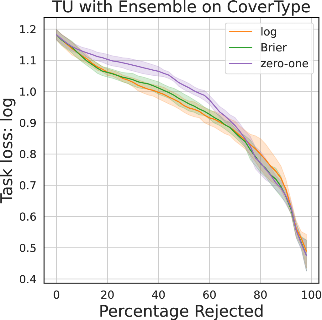
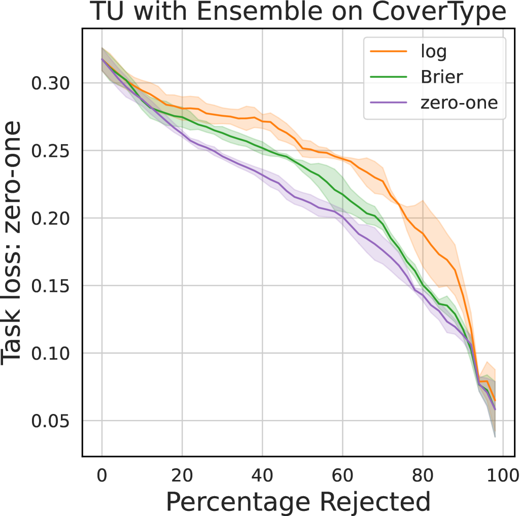
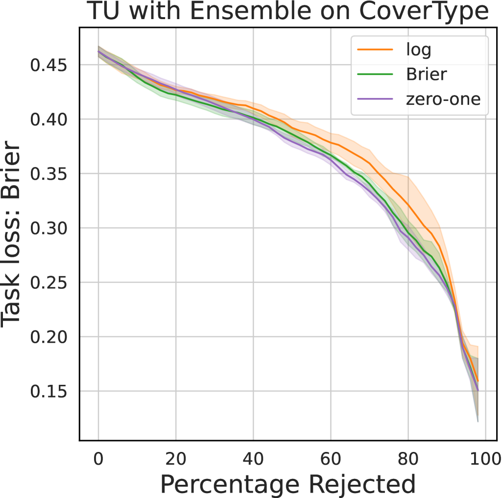
Figure 1: Selective Prediction with different task losses using the total uncertainty component as the rejection criterion. The line shows the mean and the shaded area represents the standard deviation over three runs.

5.1 Selective Prediction

We perform the selective prediction task according to the approach laid out in Section˜4. We fit a RandomForest, an ensemble of decision trees, on the CoverType dataset (Blackard, 1998). In Figure˜1 we show the results for the three different task losses using total uncertainty as the rejection criterion. This confirms our theoretical result in Section 4.2, namely that it is optimal to align the uncertainty loss with the task loss. The difference is particularly noticeable when the zero-one-loss is the underlying task loss, which is a typical loss in the selective prediction task (Nadeem et al., 2010; Geifman and El-Yaniv, 2017). In Appendix˜D we also present results using aleatoric and epistemic uncertainty as rejection criterion, highlighting that, as shown in Section˜4.2, it is best to reject instances based on total uncertainty.

Note that for probability distributions on two classes, the measures of total uncertainty induce the same ordering of the instances. Hence, for datasets where the uncertainty is limited to only a few classes, the differences between the measures may be minimal. This is the case for benchmark image datasets, such as CIFAR-10 (Krizhevsky et al., 2009), the loss-rejection curves of which we plot in Appendix˜D as an illustration.

Table 3: Out-of-Distribution detection with CIFAR-10 as in-Distribution data based on epistemic uncertainty. The mean and standard deviation over three runs are reported. Best measures are in bold.

Dataset	Method	log	Brier	zero-one
CIFAR-100	Dropout	$\textbf{0.829}\scriptstyle{\pm 0.000}$	$0.822\scriptstyle{\pm 0.000}$	$0.702\scriptstyle{\pm 0.001}$
	Ensemble	$\textbf{0.860}\scriptstyle{\pm 0.001}$	$0.852\scriptstyle{\pm 0.002}$	$0.762\scriptstyle{\pm 0.002}$
	Laplace	$\textbf{0.845}\scriptstyle{\pm 0.002}$	$0.836\scriptstyle{\pm 0.001}$	$0.808\scriptstyle{\pm 0.001}$
Places365	Dropout	$\textbf{0.837}\scriptstyle{\pm 0.001}$	$0.828\scriptstyle{\pm 0.001}$	$0.714\scriptstyle{\pm 0.002}$
	Ensemble	$\textbf{0.856}\scriptstyle{\pm 0.002}$	$0.846\scriptstyle{\pm 0.002}$	$0.758\scriptstyle{\pm 0.005}$
	Laplace	$\textbf{0.863}\scriptstyle{\pm 0.003}$	$0.850\scriptstyle{\pm 0.003}$	$0.825\scriptstyle{\pm 0.004}$
SVHN	Dropout	$\textbf{0.835}\scriptstyle{\pm 0.000}$	$0.830\scriptstyle{\pm 0.000}$	$0.701\scriptstyle{\pm 0.002}$
	Ensemble	$\textbf{0.872}\scriptstyle{\pm 0.005}$	$0.868\scriptstyle{\pm 0.005}$	$0.776\scriptstyle{\pm 0.007}$
	Laplace	$\textbf{0.865}\scriptstyle{\pm 0.005}$	$0.856\scriptstyle{\pm 0.004}$	$0.826\scriptstyle{\pm 0.006}$

5.2 Out-of-Distribution Detection

Out-of-Distribution (OoD) detection is another downstream tasks that is usually used to evaluate the representation and quantification of epistemic uncertainty. The model is trained on a dataset, which is referred to as the in-Distribution (iD) data, and then given instances from another dataset referred to as the OoD dataset. The epistemic uncertainty is computed for instances from both datasets. It is expected that a model in combination with a good uncertainty measure will exhibit higher epistemic uncertainty for the OoD data, which it has not encountered before. We compute the AUROC to show how well the iD and OoD data are separated using a given measure.

We train a ResNet18 (He et al., 2016) model on the CIFAR-10 dataset. The second-order distribution is approximated by means of an ensemble (Lakshminarayanan et al., 2017), Dropout (Gal and Ghahramani, 2016), and Laplace approximation (Daxberger et al., 2021). Table˜3 shows the performance of the three different measures of epistemic uncertainty across different OoD datasets with CIFAR-10 as the in-Distribution dataset. This demonstrates that epistemic uncertainty measures instantiated with the log-loss – specifically, mutual information – perform best. This is particularly notable, as this measure is widely used for the OoD task with second-order uncertainty representations (Mucsányi et al., 2024). In Section˜D.2 we provide additional results using the ImageNet (Deng et al., 2009) and Food101 (Bossard et al., 2014) datasets as in-Distribution datasets which further emphasize that the log-based measure performs best.

5.3 Active Learning

We use active learning as an additional task to highlight the difference between the different measures of uncertainty. In active learning the goal is to achieve good performance with as little data as possible. A learner is trained on an initial (small) pool of labeled data and can then iteratively query additional data, to be labeled by an oracle, from a (typically large) pool of unlabeled data. There exist many different strategies to query the most informative instances from the unlabeled pool, many of which are based on epistemic uncertainty (Nguyen et al., 2019; Kirsch et al., 2019; Margraf et al., 2024). Here, we also sample based on epistemic uncertainty using the epistemic uncertainty measures in Table˜2.

We use MNIST (LeCun et al., 1998) and FashionMNIST (Xiao et al., 2017) along with multi-class datasets from the MedMNIST collection (Yang et al., 2023). This collection contains both color and grayscale images. For the color images a small convolutional neural network is used based on the LeNet architecture (LeCun et al., 1998), for the grayscale images we use a small neural network with only fully-connected layers. The approximate second-order distribution is generated using dropout as is common in active learning tasks with images (Gal et al., 2017; Kirsch et al., 2019). Figure˜2 shows the zero-one-loss of the models on the test set against the number of instances used for training. For all datasets provided here, epistemic uncertainty sampling using the measure based on the zero-one-loss gives the best performance. Experiments with additional datasets are provided in Section˜D.3.

An explanation for the good performance of the zero-one-loss may be found by considering the informativeness of unlabeled instances. The unlabeled instances that provide the most information are the ones for which the model has (epistemic) uncertainty regarding the ground-truth label, as this information is only revealed upon sampling an instance. The instances for which this uncertainty does not exist, i.e. the instances for which all predicted first-order distributions “agree” on the ground-truth class, do not provide new information with respect to the label. As discussed in Section˜3, the epistemic uncertainty measure of the zero-one-loss quantifies exactly this uncertainty regarding the ground-truth class, whereas the other measures may still express epistemic uncertainty when there is no uncertainty regarding the ground-truth class.

Adjusting Measures to Prediction tasks. These experiments illustrate the importance of adjusting the uncertainty loss to the task loss, confirming our formal result from Section˜4.2. Our experiments with selective prediction in Figure˜1 also show that this task should be tackled with total uncertainty as the rejection criterion. The difference in performance of the uncertainty measures across the tasks of Out-of-Distribution detection and active learning further highlights the importance of adjusting the uncertainty measures to the downstream task. As seen in Table˜3 the log-loss-based measures provide the most reliable uncertainty measures for OoD detection, whereas for the active learning (see Figure˜2) the zero-one-loss epistemic uncertainty performs consistently better than other measures.

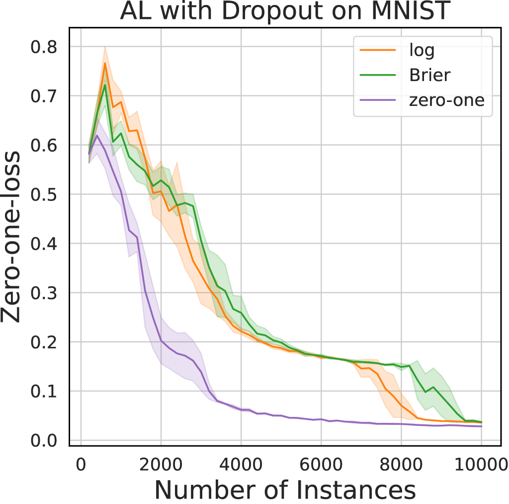
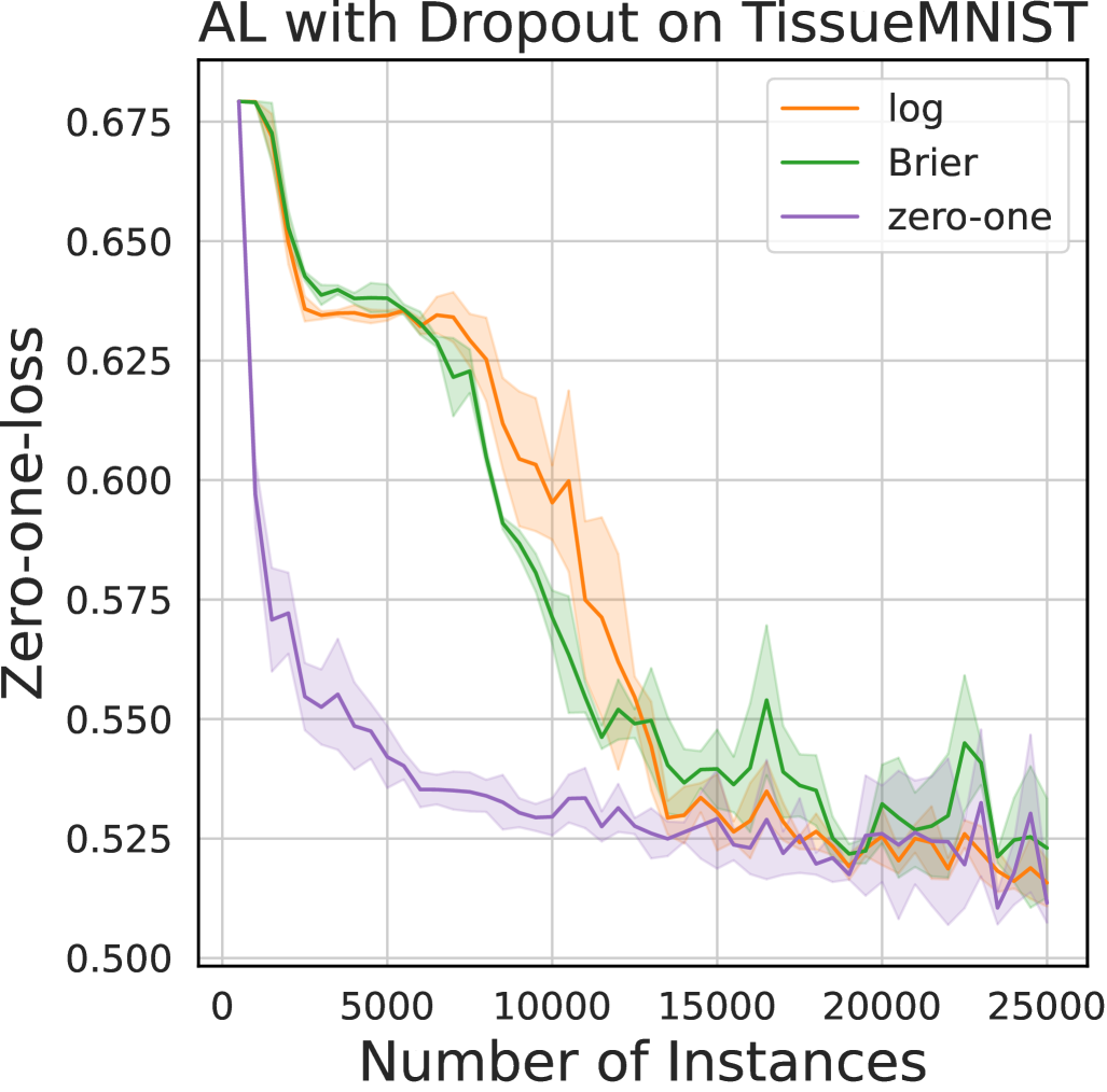
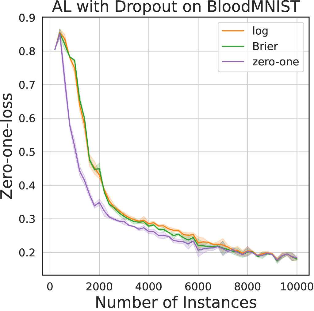
Figure 2: Active Learning with different datasets using the epistemic uncertainty component to query new instances. The model is evaluated using the zero-one-loss on the test instances. The line shows the mean and the shaded area represents the standard deviation over three runs.

6 Conclusion

In this paper, we introduced a new framework for uncertainty quantification on the basis of proper scoring rules, a specific type of loss function that facilitates a natural decomposition of total uncertainty into its aleatoric and epistemic parts. Thus, the basic idea is to define uncertainty in terms of expected loss, and the nature of the loss determines the nature of the uncertainty measure. We instantiated our method with commonly-used (strictly) proper scoring rules and showed the importance of adjusting the resulting uncertainty measures to the predictive task at hand. Through empirical evaluation we have shown that the measures generated by our decomposition offer a flexible way to perform selective prediction by adapting the uncertainty loss to the task loss. We confirmed the strong performance of the de facto standard entropy measures on Out-of-Distribution detection and presented a new measure that demonstrates consistently superior performance in active learning. Our findings emphasize that there is no universal measure of uncertainty that performs best on all tasks. We find that measures performing well on the Out-of-Distribution task may not work best for the active learning task. The choice of a specific measure can be supported by considering the task loss in the case of selective prediction or by focusing on the uncertainty that is relevant for the particular task in the case of OoD and active learning.

Limitations and Future Work. In this work we have assumed that we are given a second-order distribution without explicitly focusing on how it was learned. The learning process involves an additional training loss that we have not discussed here. Future work could explore the connection between the (proper) loss used during training of model and the performance of uncertainty measures on specific downstream tasks. Given such a trained model that predicts a second-order distribution, the characteristics of the different second-order distributions predicted by different uncertainty representation method also plays a significant role. Dropout will result in a different uncertainty representation than Laplace approximation. The interaction between the second-order distribution and the uncertainty measures presents a promising avenue for future work. Lastly, we have explicitly focused our analysis on the selective prediction task here. However, other downstream tasks, such as Out-of-Distribution detection and active learning, should also be explored further to investigate why certain uncertainty losses and components result in better downstream performance.

Broader Impacts. This work contributes to the development of more reliable machine learning models by improving uncertainty quantification. We do not foresee any direct negative broader impacts arising from this work.

Appendix A Derivations

In this section, we derive total, aleatoric and epistemic uncertainty measures instantiated with log, Brier, zero-one, and spherical loss, respectively. To begin, recall the following definitions:

$$\operatorname{TU}(Q) =\mathbb{E}_{\bm{\theta}\sim Q}[L_{\ell}(\bar{\bm{\theta}},\bm{\theta})]=\mathbb{E}_{\bm{\theta}\sim Q}[\mathbb{E}_{y\sim\bm{\theta}}[\ell(\bar{\bm{\theta}},y)]]$$ (8)

$$\operatorname{AU}(Q) =\mathbb{E}_{\bm{\theta}\sim Q}[H_{\ell}(\bm{\theta})]=\mathbb{E}_{\bm{\theta}\sim Q}[L_{\ell}(\bm{\theta},\bm{\theta})]=\mathbb{E}_{\bm{\theta}\sim Q}[\mathbb{E}_{y\sim\bm{\theta}}[\ell(\bm{\theta},y)]]$$ (9)

$$\operatorname{EU}(Q) =\mathbb{E}_{\bm{\theta}\sim Q}[D_{\ell}(\bar{\bm{\theta}},\bm{\theta})]=\mathbb{E}_{\bm{\theta}\sim Q}[L_{\ell}(\bar{\bm{\theta}},\bm{\theta})-L_{\ell}(\bm{\theta},\bm{\theta})]=\mathbb{E}_{\bm{\theta}\sim Q}[\mathbb{E}_{y\sim\bm{\theta}}[\ell(\bar{\bm{\theta}},y)-\ell(\bm{\theta},y)]]$$ (10)

A.1 Log-loss

With $\ell(\bar{\bm{\theta}},y)=-\log(\bar{\bm{\theta}}_{y})$,

$$\operatorname{TU}(Q) =\mathbb{E}_{\bm{\theta}\sim Q}[\mathbb{E}_{y\sim\bm{\theta}}[-\log(\bar{\theta}_{y})]]$$

$$=\mathbb{E}_{\bm{\theta}\sim Q}[\sum_{k=1}^{K}\theta_{k}(-\log(\bar{\theta}_{k}))]$$

$$=\sum_{k=1}^{K}\bar{\theta}_{k}(-\log(\bar{\theta}_{k}))$$

$$=S(\bar{\bm{\theta}}),$$

$$\operatorname{AU}(Q) =\mathbb{E}_{\bm{\theta}\sim Q}[\mathbb{E}_{y\sim\bm{\theta}}[-\log(\theta_{y})]]$$

$$=\mathbb{E}_{\bm{\theta}\sim Q}[S(\bm{\theta})],$$

$$\operatorname{EU}(Q) =\mathbb{E}_{\bm{\theta}\sim Q}[\mathbb{E}_{y\sim\bm{\theta}}[-\log(\bar{\theta}_{y})+\log(\theta_{y})]]$$

$$=\mathbb{E}_{\bm{\theta}\sim Q}[\operatorname{KL}(\bm{\theta}\parallel\bar{\bm{\theta}})].$$

A.2 Brier-loss

With $\ell(\bar{\bm{\theta}},y)=\sum_{k=1}^{K}(\bar{\theta}_{k}-\llbracket k=y\rrbracket)^{2}=-2\bar{\theta}_{y}+\sum_{k=1}^{K}\bar{\theta}_{k}^{2}+1$,

$$\operatorname{TU}(Q) =\mathbb{E}_{\bm{\theta}\sim Q}[\mathbb{E}_{y\sim\bm{\theta}}[-2\bar{\theta}_{y}+\sum_{k=1}^{K}\bar{\theta}_{k}^{2}+1]]$$

$$=\mathbb{E}_{\bm{\theta}\sim Q}[\sum_{k=1}^{K}\theta_{k}(-2\bar{\theta}_{k})]+\sum_{k=1}^{K}\bar{\theta}_{k}^{2}+1$$

$$=\sum_{k=1}^{K}\bar{\theta}_{k}(-2\bar{\theta}_{k})+\sum_{k=1}^{K}\bar{\theta}_{k}^{2}+1$$

$$=\sum_{k=1}^{K}-2\bar{\theta}_{k}^{2}+\sum_{k=1}^{K}\bar{\theta}_{k}^{2}+1$$

$$=1-\sum_{k=1}^{K}\bar{\theta}_{k}^{2},$$

$$\operatorname{AU}(p) =\mathbb{E}_{\bm{\theta}\sim Q}[\mathbb{E}_{y\sim\bm{\theta}}[-2\theta_{y}+\sum_{k=1}^{K}\theta_{k}^{2}+1]]$$

$$=\mathbb{E}_{\bm{\theta}\sim Q}[\sum_{k=1}^{K}\theta_{k}(-2\theta_{k})+\sum_{k=1}^{K}\theta_{k}^{2}+1]$$

$$=\mathbb{E}_{\bm{\theta}\sim Q}[\sum_{k=1}^{K}-2\theta_{k}^{2}+\sum_{k=1}^{K}\theta_{k}^{2}+1)]$$

$$=\mathbb{E}_{\bm{\theta}\sim Q}[1-\sum_{k=1}^{K}\theta_{k}^{2}],$$

$$\operatorname{EU}(p) =\mathbb{E}_{\bm{\theta}\sim Q}[\mathbb{E}_{y\sim\bm{\theta}}[-2\bar{\theta}_{y}+\sum_{k=1}^{K}\bar{\theta}_{k}^{2}+1+2\theta_{y}-\sum_{k=1}^{K}\theta_{k}^{2}-1]]$$

$$=\mathbb{E}_{\bm{\theta}\sim Q}[\sum_{k=1}^{K}\theta_{k}(-2\bar{\theta}_{k}+2\theta_{k})+\sum_{k=1}^{K}\bar{\theta}_{k}^{2}-\sum_{k=1}^{K}\theta_{k}^{2}]$$

$$=\mathbb{E}_{\bm{\theta}\sim Q}[\sum_{k=1}^{K}(-2\bar{\theta}_{k}\theta_{k}+2\theta_{k}^{2})+\sum_{k=1}^{K}\bar{\theta}_{k}^{2}-\sum_{k=1}^{K}\theta_{k}^{2}]$$

$$=\mathbb{E}_{\bm{\theta}\sim Q}[\sum_{k=1}^{K}(\bar{\theta}_{k}^{2}-2\bar{\theta}_{k}\theta_{k}+\theta_{k}^{2})]$$

$$=\mathbb{E}_{\bm{\theta}\sim Q}[\sum_{k=1}^{K}(\bar{\theta}_{k}^{2}-\theta_{k}^{2})].$$

A.3 Zero-one-loss

With $\ell(\bar{\bm{\theta}},y)=1-\llbracket\operatorname*{arg\,max}_{k}\bar{\theta}_{k}=y\rrbracket$,

$$\operatorname{TU}(Q) =\mathbb{E}_{\bm{\theta}\sim Q}[\mathbb{E}_{y\sim\bm{\theta}}[1-\llbracket\operatorname*{arg\,max}_{k}\bar{\theta}_{k}=y\rrbracket]$$

$$=\mathbb{E}_{\bm{\theta}\sim Q}[\sum_{k^{\prime}=1}^{K}\theta_{k^{\prime}}(1-\llbracket\operatorname*{arg\,max}_{k}\bar{\theta}_{k}=k^{\prime}\rrbracket)$$

$$=\sum_{k^{\prime}=1}^{K}\bar{\theta}_{k^{\prime}}(1-\llbracket\operatorname*{arg\,max}_{k}\bar{\theta}_{k}=k^{\prime}\rrbracket)$$

$$=1-\max_{k}\bar{\theta}_{k},$$

$$\operatorname{AU}(Q) =\mathbb{E}_{\bm{\theta}\sim Q}[\mathbb{E}_{y\sim\bm{\theta}}[1-\llbracket\operatorname*{arg\,max}_{k}\theta_{k}=y\rrbracket]$$

$$=\mathbb{E}_{\bm{\theta}\sim Q}[1-\max_{k}\theta_{k}],$$

$$\operatorname{EU}(Q) =\mathbb{E}_{\bm{\theta}\sim Q}[\mathbb{E}_{y\sim\bm{\theta}}[1-\llbracket\operatorname*{arg\,max}_{k}\bar{\theta}_{k}=y\rrbracket]-1+\llbracket\operatorname*{arg\,max}_{k}\theta_{k}=y\rrbracket]$$

$$=\mathbb{E}_{\bm{\theta}\sim Q}[\mathbb{E}_{y\sim\bm{\theta}}[\llbracket\operatorname*{arg\,max}_{k}\theta_{k}=y\rrbracket]-\llbracket\operatorname*{arg\,max}_{k}\bar{\theta}_{k}=y\rrbracket]$$

$$=\mathbb{E}_{\bm{\theta}\sim Q}[\max_{k}\theta_{k}-\theta_{\operatorname*{arg\,max}_{k}\bar{\theta}_{k}}].$$

A.4 Spherical-loss

With $\ell(\bar{\bm{\theta}},y)=1-\frac{\hat{\theta}_{y}}{\|\bar{\bm{\theta}}\|_{2}}$,

$$\operatorname{TU}(Q) =\mathbb{E}_{\bm{\theta}\sim Q}[\mathbb{E}_{y\sim\bm{\theta}}[1-\frac{\bar{\theta}_{k}}{\|\bar{\bm{\theta}}\|_{2}}]]$$

$$=\mathbb{E}_{\bm{\theta}\sim Q}[1-\frac{\sum_{k=1}^{K}\theta_{k}\bar{\theta}_{k}}{\|\bar{\bm{\theta}}\|_{2}}]$$

$$=1-\frac{\sum_{k=1}^{K}\bar{\theta}^{2}}{\|\bar{\bm{\theta}}\|_{2}}$$

$$=1-\|\bar{\bm{\theta}}\|_{2},$$

$$\operatorname{AU}(Q) =\mathbb{E}_{\bm{\theta}\sim Q}[\mathbb{E}_{y\sim\bm{\theta}}[1-\frac{\theta_{k}}{\|\bm{\theta}\|_{2}}]]$$

$$=\mathbb{E}_{\bm{\theta}\sim Q}[1-\frac{\sum_{k=1}^{K}\theta_{k}^{2}}{\|\bm{\theta}\|_{2}}]$$

$$=\mathbb{E}_{\bm{\theta}\sim Q}[1-\|\bm{\theta}\|_{2}],$$

$$\operatorname{EU}(Q) =\mathbb{E}_{\bm{\theta}\sim Q}[\mathbb{E}_{y\sim\bm{\theta}}[1-\frac{\bar{\theta}_{k}}{\|\bar{\bm{\theta}}\|_{2}}-1+\frac{\theta_{k}}{\|\bm{\theta}\|_{2}}]]$$

$$=\mathbb{E}_{\bm{\theta}\sim Q}[\mathbb{E}_{y\sim\bm{\theta}}[\frac{\theta_{k}}{\|\bm{\theta}\|_{2}}-\frac{\bar{\theta}_{k}}{\|\bar{\bm{\theta}}\|_{2}}]]$$

$$=\mathbb{E}_{\bm{\theta}\sim Q}[\frac{\sum_{k=1}^{K}\theta_{k}^{2}}{\|\bm{\theta}\|_{2}}-\frac{\sum_{k=1}^{K}\bar{\theta}_{k}\theta_{k}}{\|\bar{\bm{\theta}}\|_{2}}]$$

$$=\mathbb{E}_{\bm{\theta}\sim Q}[\|\bm{\theta}\|_{2}-\frac{\sum_{k=1}^{K}\bar{\theta}_{k}\theta_{k}}{\|\bar{\bm{\theta}}\|_{2}}].$$

Appendix B Proofs

Proof of proposition 4.1.

For $\alpha\in[0,1]$, the area under the loss-rejection curve (AULC) is defined as

$$\rm{AULC}=\int_{0}^{1}\left(\frac{1}{\lfloor\alpha n\rfloor}\sum_{j=1}^{\lfloor\alpha n\rfloor}\ell(\hat{\theta}_{\pi(j)},y_{\pi(j)})\right)\,d\alpha.$$

Define $c_{\pi(j)}\coloneqq\mathbb{E}\bigl{[}\ell(\hat{\theta}_{\pi(j)},y_{\pi(j)})\bigr{]}$. Then, the expected area under the loss-rejection curve is given by

$$\mathbb{E}[\mathrm{AULC}] =\int_{0}^{1}\left(\frac{1}{\lfloor\alpha n\rfloor}\sum_{j=1}^{\lfloor\alpha n\rfloor}\mathbb{E}\bigl{[}\ell(\hat{\theta}_{\pi(j)},y_{\pi(j)})\bigr{]}\right)d\alpha=\int_{0}^{1}\left(\frac{1}{\lfloor\alpha n\rfloor}\sum_{j=1}^{\lfloor\alpha n\rfloor}c_{\pi(j)}\right)d\alpha.$$

Consequently, we can approximate the integral by a Riemann sum with step $\Delta\alpha=\frac{1}{n}$:

$$\mathbb{E}[\mathrm{AULC}]\approx\frac{1}{n}\underbrace{\sum_{k=1}^{n}\left(\frac{1}{k}\sum_{j=1}^{k}c_{\pi(j)}\right)}_{\eqqcolon S({\pi})}.$$

Then, interchanging the order of summation yields

$$S(\pi)=\sum_{k=1}^{n}\sum_{j=1}^{k}\frac{1}{k}\,c_{\pi(j)}=\sum_{j=1}^{n}c_{\pi(j)}\sum_{k=j}^{n}\frac{1}{k}.$$

With weights $w_{j}=\sum_{k=j}^{n}\frac{1}{k}$ we finally get $S(\pi)=\sum_{j=1}^{n}w_{j}\,c_{\pi(j)}$. Since $w_{1}\geq w_{2}\geq\cdots\geq w_{n}>0$, the rearrangement inequality implies that the sum $\sum_{j=1}^{n}w_{j}\,c_{\pi(j)}$ is minimized when $c_{\pi(1)}\leq c_{\pi(2)}\leq\cdots\leq c_{\pi(n)}$.

This completes the proof. ∎

Appendix C Experimental Details

In the following, we will provide additional details regarding the experimental setup. We split this into details about the models and training setup, the uncertainty methods and how they are applied, and details about the downstream tasks. The code is written in Python 3.10.12 and relies heavily on PyTorch [Paszke et al., 2019].

C.1 Compute Resources

The experiments were conducted using the compute resources in Table˜4. The presented results were computed in approximately 50 GPU hours and 10 additional CPU hours.

Table 4: Compute Resources.

Resource	Details
GPU	2x NVIDIA A40 48GB GDDR
CPU	AMD EPYC MILAN 7413 24 Cores / 48 Threads
RAM	128GB DDR4-3200MHz ECC DIMM
Storage	2x 480GB Samsung Datacenter SSD PM893

C.2 Datasets

Table 5: Datasets with references and licenses.

Dataset	Reference	License
CoverType	[Blackard, 1998]	CC BY.
Poker Hand	[Cattral and Oppacher, 2006]	CC BY.
CIFAR-10	Krizhevsky et al. [2009]	Unknown.
CIFAR-100	[Krizhevsky et al., 2009]	Unknown.
Places365	[Zhou et al., 2018]	CC BY.
SVHN	[Netzer et al., 2011]	Non-commercial use.
ImageNet	[Deng et al., 2009]	Non-commerical research/educational use.
ImageNet-O	[Hendrycks et al., 2021]	MIT License.
Food101	[Bossard et al., 2014]	Unknown.
MNIST	[LeCun et al., 1998]	CC BY.
FashionMNIST	[Xiao et al., 2017]	MIT License.
MedMNIST	[Yang et al., 2023]	CC BY.

Table 5 lists all datasets that we use to generate the results. We use the dedicated train-test split for all datasets when available. The CoverType and Poker Hand datasets do not have a dedicated train-test split, hence we use a $70\%-30\%$ split. During training, CIFAR-10 is normalized using the training set mean and standard deviation per channel, and random cropping and horizontal flipping is applied. For Out-of-Distribution all iD and OoD instances undergo the same transformations.

C.3 Models

We train the following models.

Random Forest.

The RandomForest is fit on CoverType using 20 trees and a maximum depth of 5 and on Poker Hand with 20 trees and a maximum depth of 20. For the remaining hyper-parameters, we use the defaults provided by sklearn [Pedregosa et al., 2011].

Multilayer Perceptron.

The Multilayer Perceptron (MLP) consists of an input layer with 784 features with ReLU activations followed by a hidden layer with 100 features and ReLU activation, and an output layer whose size corresponds to the number of classes after which a softmax function is applied.

Convolutional Neural Network.

The Convolutional Neural Network (CNN) is based on the LeNet5 architecture [LeCun et al., 1998]. It takes a three-channel input and consists of two convolutional layers followed by two fully-connected layers. The first convolutional layer has 32 filters of size 5x5 and the second has 64 filters of size 5x5. Both layers are followed by a 2x2 max-pooling operation and a ReLU activation. The feature maps are flattened and passed to the first fully-connected layer with 800 features and ReLU activation. Finally, the size of the output layer depends on the number of classes and applies a softmax function.

The training hyper-parameters of the models depend on the dataset and are listed in Table˜6.

ResNet.

We use the ResNet18 [He et al., 2016] implementation from https://github.com/kuangliu/pytorch-cifar for the CIFAR-10 experiments. The ResNets are trained for 100 epochs using stochastic gradient descent with a learning rate of 0.001, weight decay at 5e-4 and momentum at 0.9. The cosine annealing learning rate scheduler [Loshchilov and Hutter, 2017] is used.

We use the following pre-trained models.

EfficientNet.

For the ImageNet experiments, we use the EfficientNetV2S implementation from PyTorch which was pre-trained on ImageNet.

VisionTransformer.

We use a VisionTransformer for the Food101 experiments. It was pre-trained on Imagenet21K [Ridnik et al., 2021] and fine-tuned on Food101. It was downloaded from Hugging Face https://huggingface.co/nateraw/vit-base-food101.

C.4 Uncertainty Representations

The following methods are used to enable the models to represent their uncertainty using second-order distributions or approximations thereof.

Dropout.

A Dropout layer before the final layer using the default probability $0.5$ from PyTorch is used. The other Dropout layers are turned off during evaluation.

Laplace Approximation.

We use the Laplace package [Daxberger et al., 2021] to fit the Laplace approximation on the last layer using the Kronecker-factored approximate curvature approximation, which are the default settings for this package. We obtain samples of the posterior by Monte Carlo sampling.

Deep Ensembles.

The deep ensemble is constructed by training 5 similar neural networks, relying on the randomness of the initialization and stochastic gradient descent to get diverse predictions [Lakshminarayanan et al., 2017].

C.5 Downstream Tasks

All tasks are run three times and for each run a new model is trained (only exception being pre-trained Dropout and Laplace models) and a random subset of the test data is sampled. For the downstream tasks, given an instance, we sample 20 conditional distributions in order to compute the total, aleatoric and epistemic uncertainty.

Selective Prediction.

The selective prediction tasks are done using 10,000 instances that are randomly sampled from the dedicated test split of the datasets.

Out-of-Distribution Detection.

For the Out-of-Distribution Detection task we also sample 10,000 instances from the test sets of the respective datasets, if possible. ImageNet-O has only 2,000 instances, thus we use all these instances and also sample 2,000 instances from the in-Distribution dataset.

Active Learning.

Active learning is performed by starting with training on only the initial instances. The model then uses epistemic uncertainty to sample new instances with a certain query budget. After this, the model is trained again and the performance on the dedicated test set of the respective dataset is evaluated. This process is repeated for 50 iterations. The settings used for the different datasets are shown in Table˜6.

Table 6: Setting for the active learning experiments.

Dataset	Initial Instances	Query Budget	Learning Rate	Epochs
MNIST	100	100	0.01	50
TissueMNIST	500	500	0.01	50
BloodMNIST	200	200	0.001	100
FashionMNIST	500	500	0.01	50
OrganCMNIST	200	200	0.01	50
PathMNIST	1000	1000	0.001	100

Appendix D Additional Results

D.1 Selective Prediction

We present the selective prediction results for the CoverType dataset with total and aleatoric uncertainty as the rejection criteria in Figure˜3, confirming that the best performance is obtained by using total uncertainty as the rejection criterion.

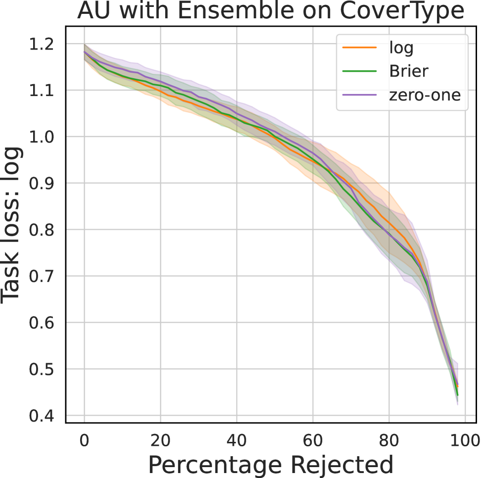
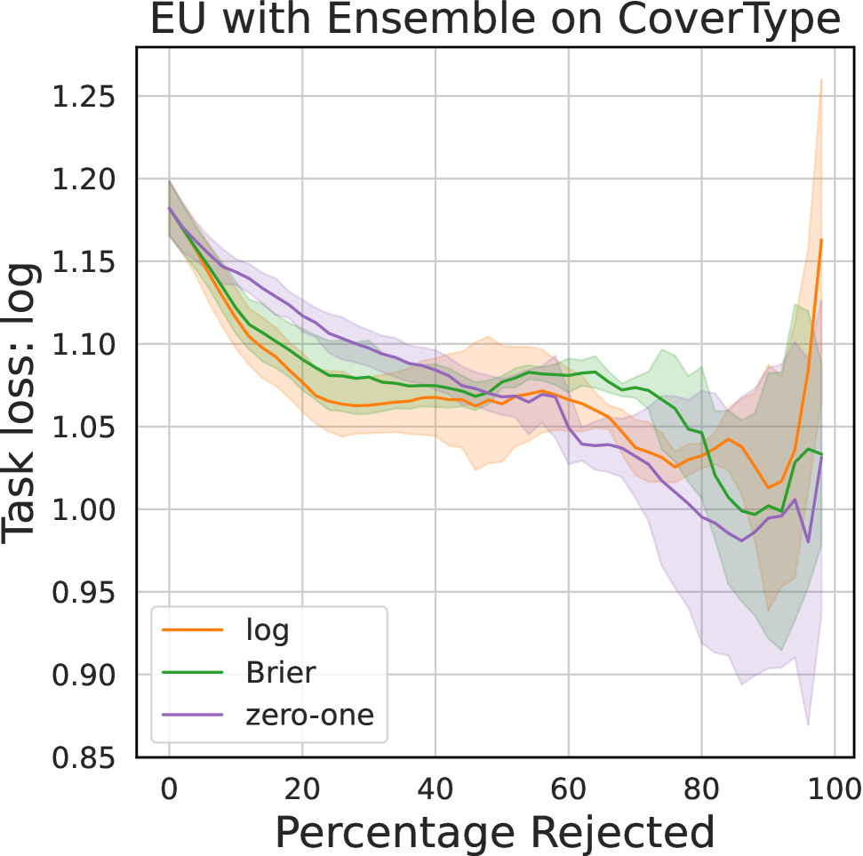
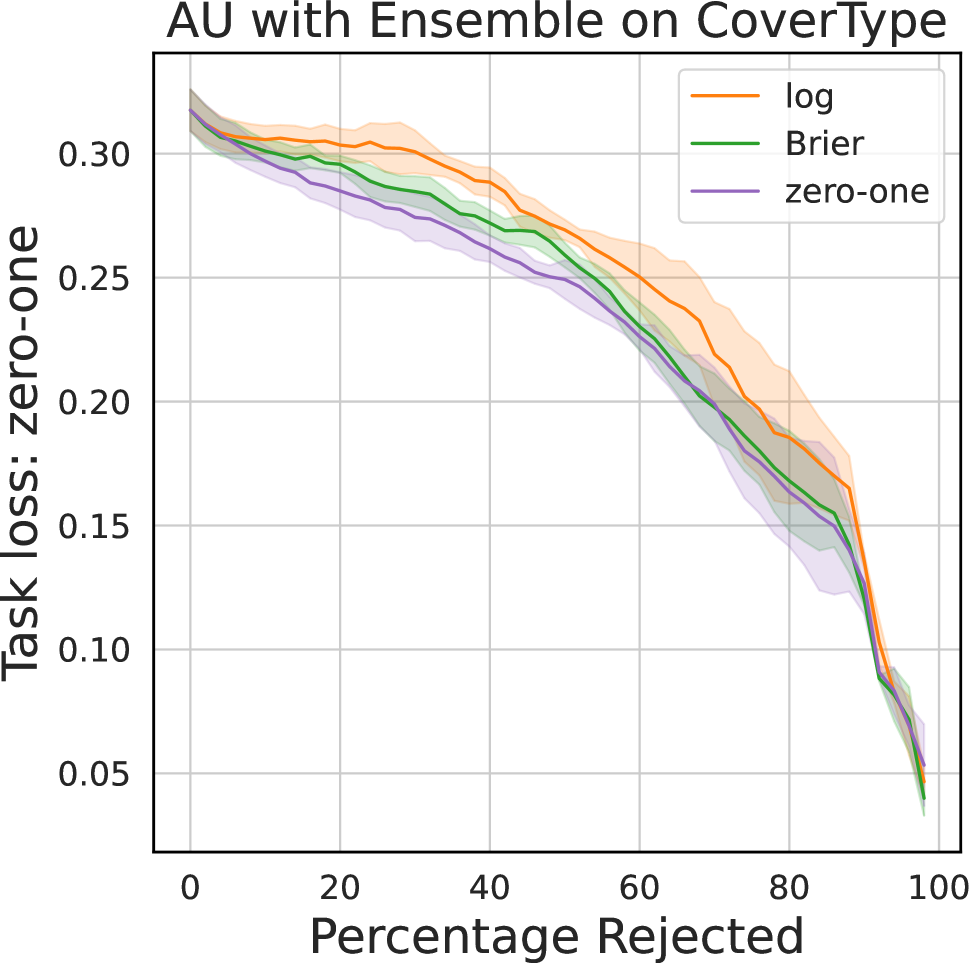
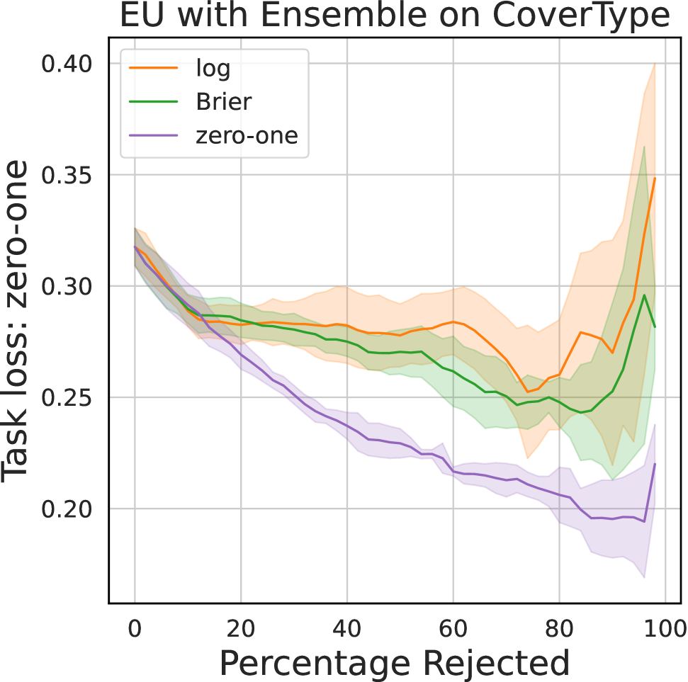
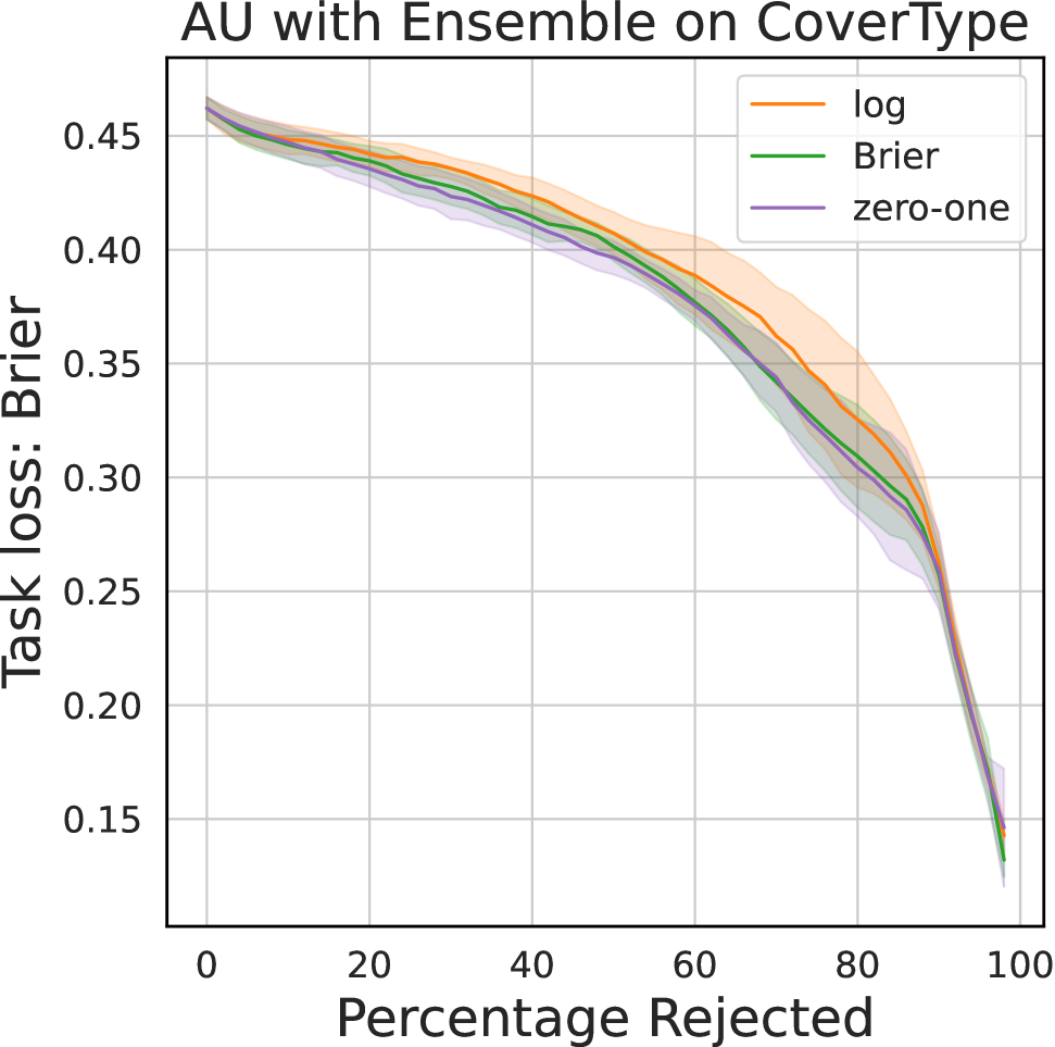
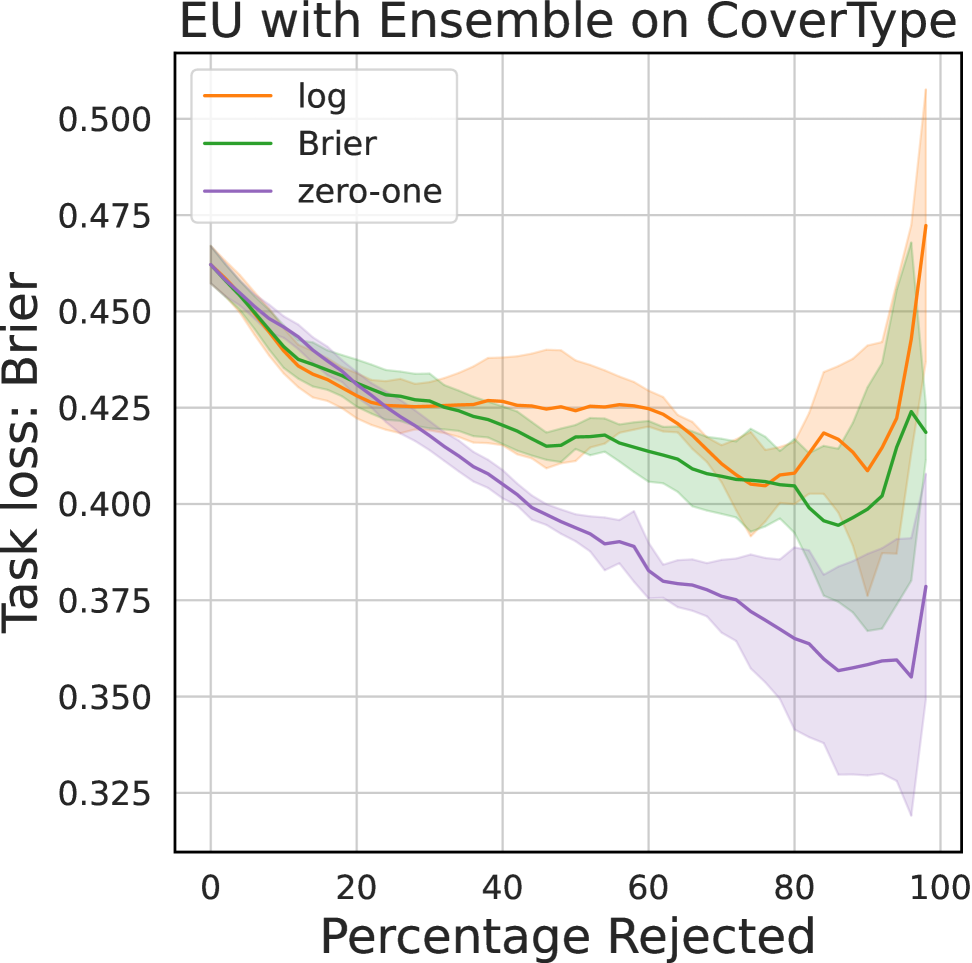
Figure 3: Selective Prediction with different task losses using the aleatoric uncertainty (top row) and epistemic uncertainty (bottom row) component as the rejection criterion. The line shows the mean and the shaded area represents the standard deviation over three runs.

We also present selective prediction results for the Poker Hand dataset with total, aleatoric, and epistemic in Figure˜4. These results show the same behavior as for the CoverType dataset.

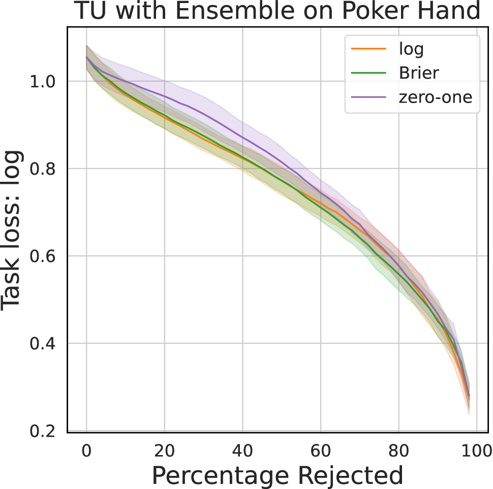
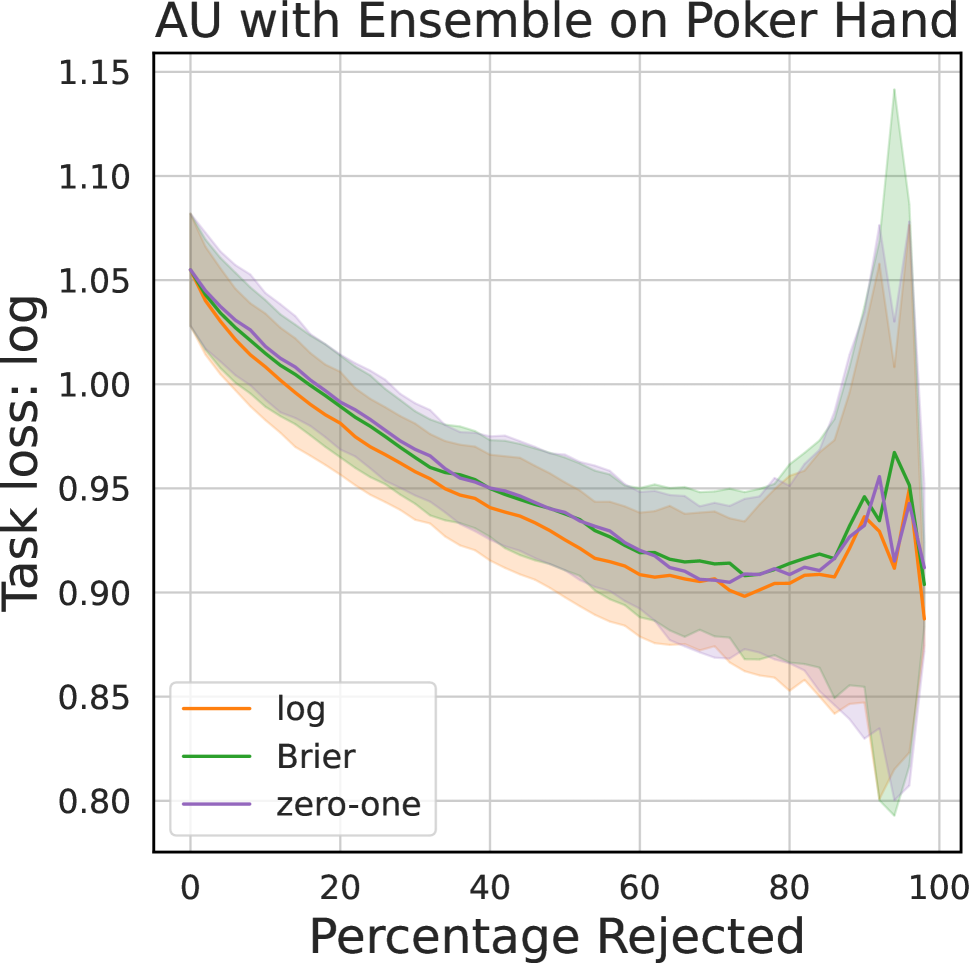
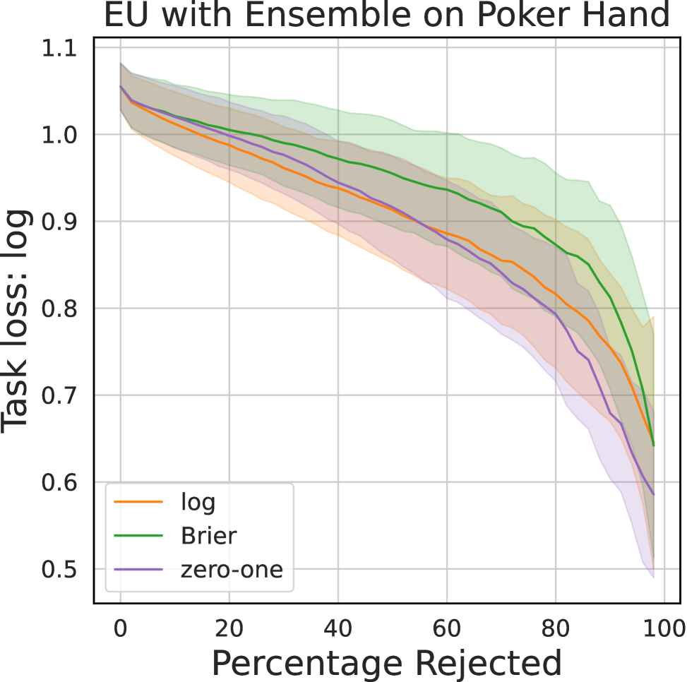
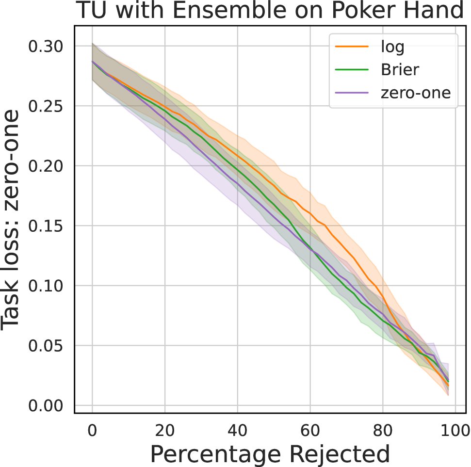
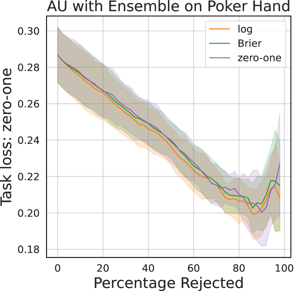
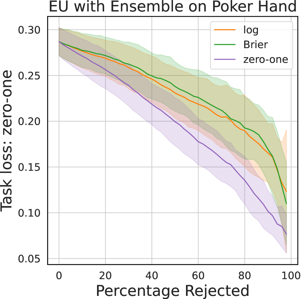
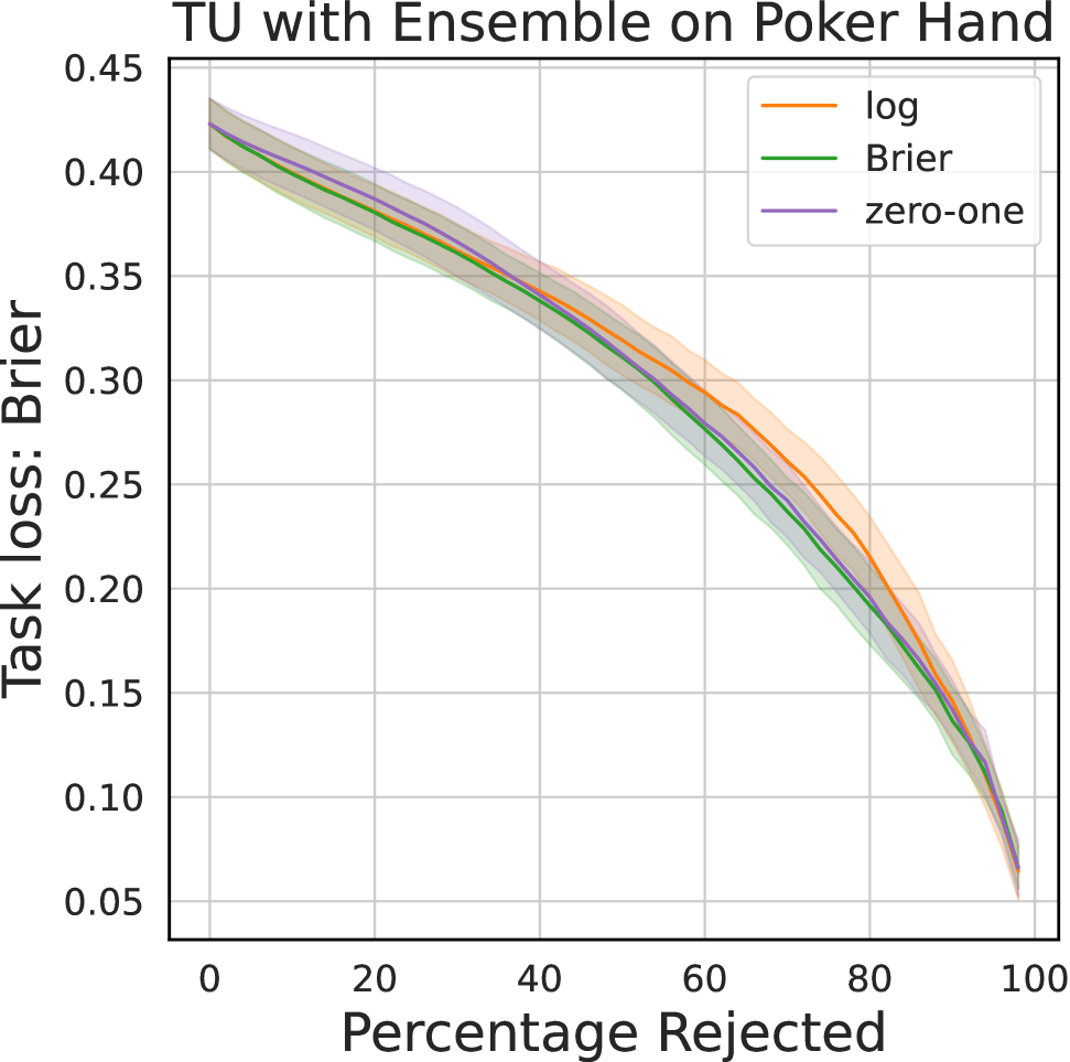
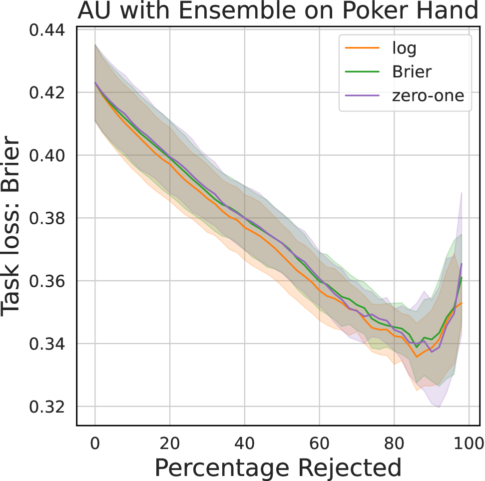
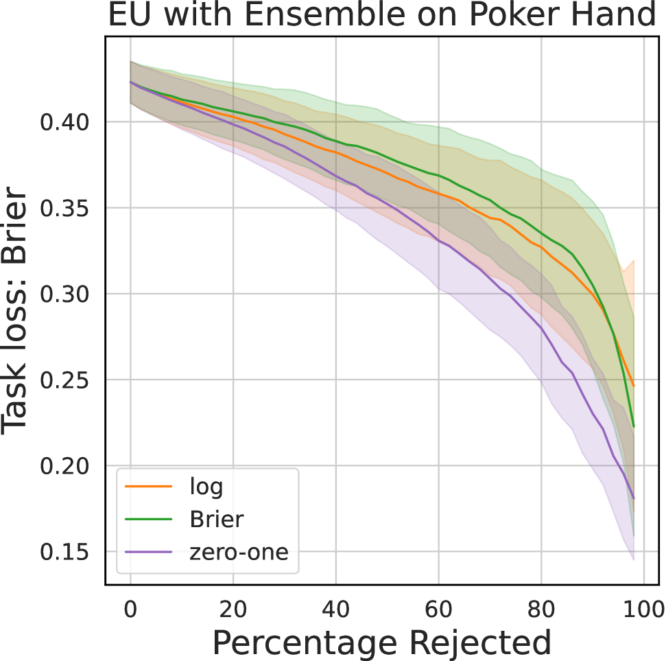
Figure 4: Selective Prediction with different task losses using the total uncertainty (top row), aleatoric uncertainty (middle row) and epistemic uncertainty (bottom row) component as the rejection criterion. The line shows the mean and the shaded area represents the standard deviation over three runs.

In addition, we present selective prediction results for the CIFAR-10 dataset using total uncertainty as the rejection criterion in Figure˜5. As mentioned, the cumulative probability of the top-2 classes across the test instances is $0.989\pm 0.042$, which explains the similar behavior for the uncertainty measures.

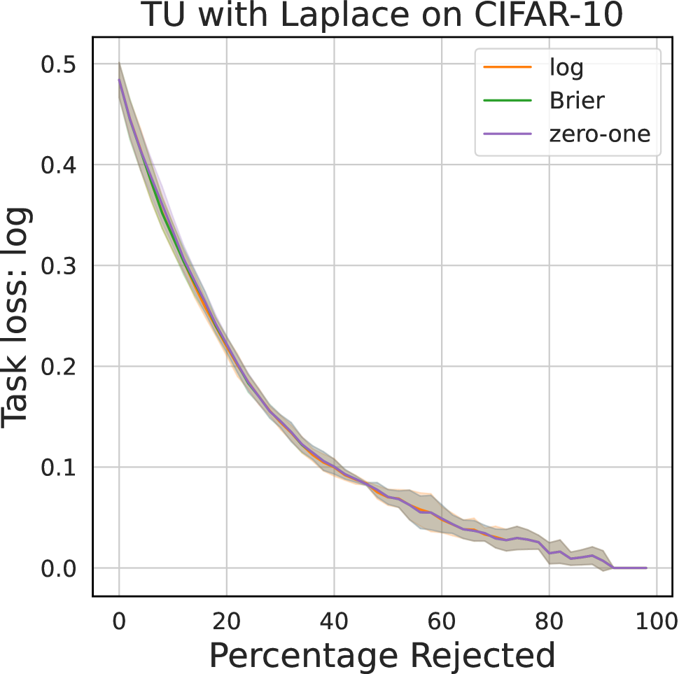
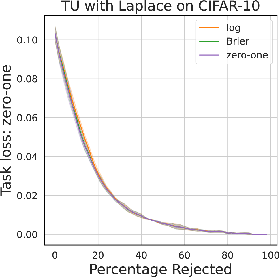
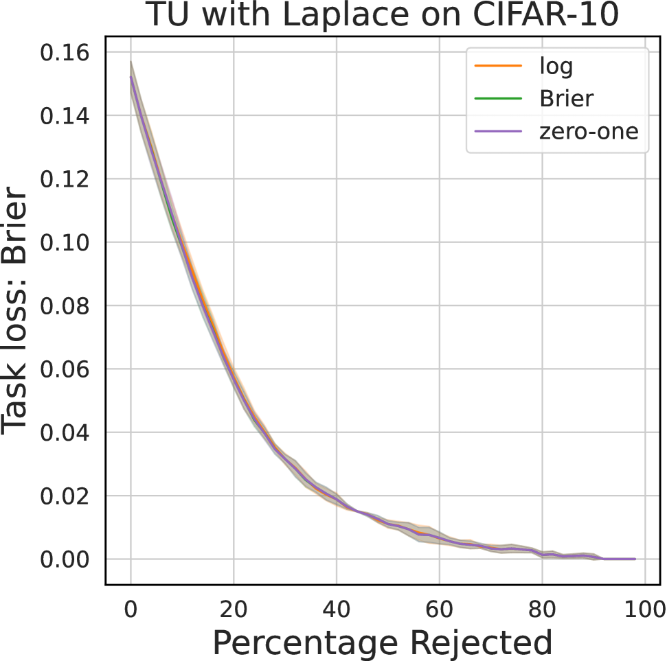
Figure 5: Selective Prediction with different task losses using the aleatoric uncertainty (top row) and epistemic uncertainty (bottom row) component as the rejection criterion. The line shows the mean and the shaded area represents the standard deviation over three runs.

We provide selective prediction results for the CoverType dataset using the total uncertainty based on the spherical loss in Figure˜6. The spherical loss, a strictly proper scoring rule, is not discussed in the main paper as it is not as common as the log-loss, Brier-loss or zero-one-loss. The derivations of the uncertainty measures for this loss can be found in Appendix˜A.

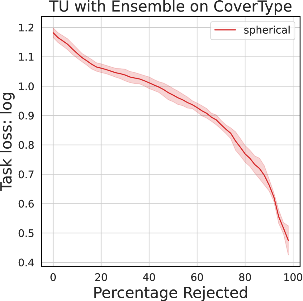
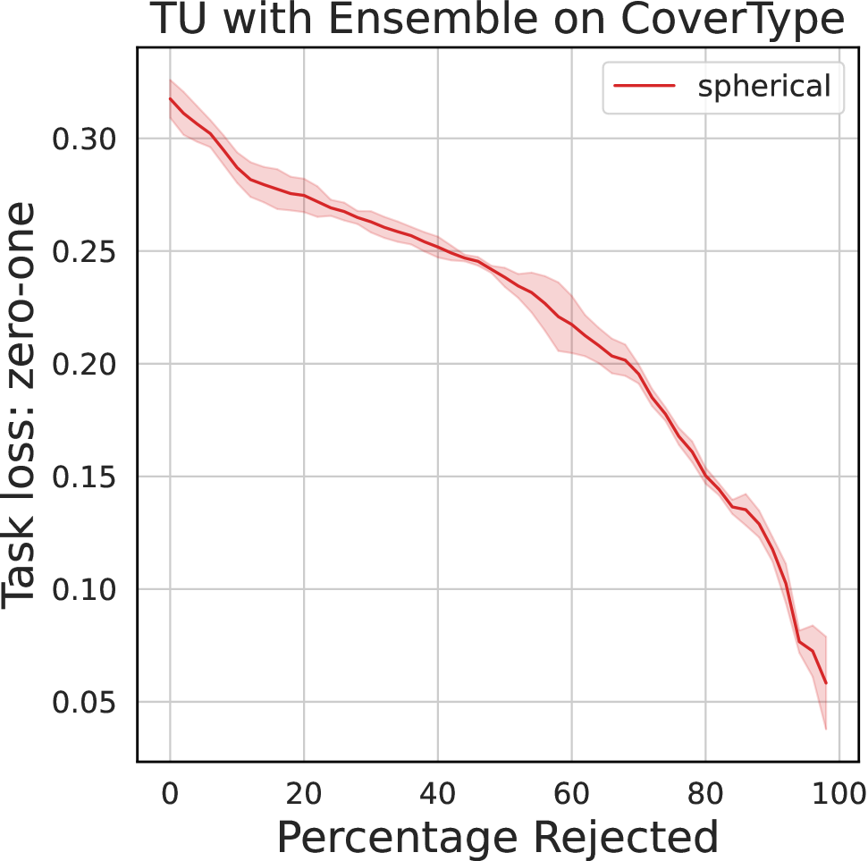
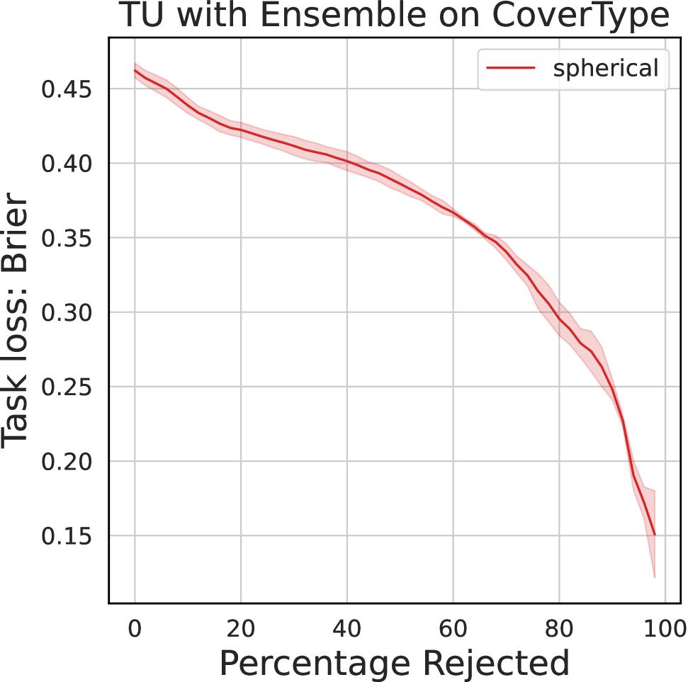
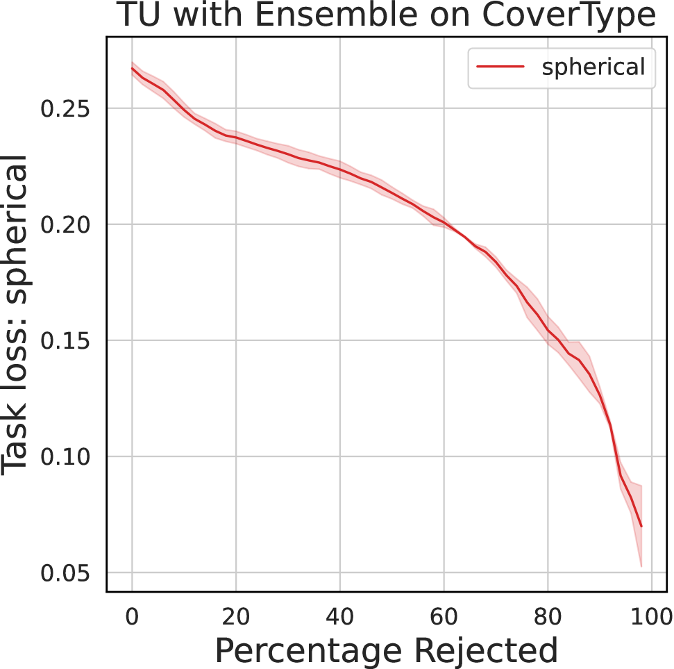
Figure 6: Selective Prediction with different task losses using the total uncertainty component as the rejection criterion. The line shows the mean and the shaded area represents the standard deviation over three runs.

D.2 Out-of-Distribution Detection

We present additional Out-of-Distribution results for the ImageNet and Food101 datasets with different uncertainty representations in Table˜7 and Table˜8, respectively. This confirms that mutual information, the log-based epistemic uncertainty measure performs best for the Out-of-Distribution downstream task. Additionally, we provide Out-of-Distribution results for the CIFAR-10 dataset using epistemic uncertainty based on the spherical loss in Table˜9. Comparing these results to the ones presented in Table˜3 confirms that mutual information performs best, as mentioned before.

Table 7: Out-of-Distribution detection with ImageNet as in-Distribution data based on epistemic uncertainty. The mean and standard deviation over three runs are reported. Best measures are in bold.

Dataset	Method	log	Brier	zero-one
ImageNet-O	Dropout	$\textbf{0.711}\scriptstyle{\pm 0.009}$	$0.688\scriptstyle{\pm 0.008}$	$0.550\scriptstyle{\pm 0.006}$
	Laplace	$\textbf{0.789}\scriptstyle{\pm 0.006}$	$0.713\scriptstyle{\pm 0.005}$	$0.678\scriptstyle{\pm 0.008}$
CIFAR-100	Dropout	$\textbf{0.876}\scriptstyle{\pm 0.002}$	$0.753\scriptstyle{\pm 0.002}$	$0.721\scriptstyle{\pm 0.002}$
	Laplace	$\textbf{0.935}\scriptstyle{\pm 0.001}$	$0.892\scriptstyle{\pm 0.002}$	$0.894\scriptstyle{\pm 0.002}$
Places365	Dropout	$\textbf{0.809}\scriptstyle{\pm 0.001}$	$0.744\scriptstyle{\pm 0.001}$	$0.671\scriptstyle{\pm 0.001}$
	Laplace	$\textbf{0.811}\scriptstyle{\pm 0.001}$	$0.732\scriptstyle{\pm 0.003}$	$0.780\scriptstyle{\pm 0.002}$
SVHN	Dropout	$\textbf{0.969}\scriptstyle{\pm 0.001}$	$0.580\scriptstyle{\pm 0.002}$	$0.857\scriptstyle{\pm 0.002}$
	Laplace	$\textbf{0.994}\scriptstyle{\pm 0.000}$	$0.956\scriptstyle{\pm 0.001}$	$0.983\scriptstyle{\pm 0.001}$

Table 8: Out-of-Distribution detection with Food101 as in-Distribution data based on epistemic uncertainty. The mean and standard deviation over three runs are reported. Best measures are in bold.

Dataset	Method	log	Brier	zero-one
CIFAR-100	Dropout	$\textbf{0.990}\scriptstyle{\pm 0.000}$	$0.802\scriptstyle{\pm 0.002}$	$0.921\scriptstyle{\pm 0.001}$
	Laplace	$\textbf{0.998}\scriptstyle{\pm 0.000}$	$0.996\scriptstyle{\pm 0.000}$	$0.997\scriptstyle{\pm 0.000}$
Places365	Dropout	$\textbf{0.987}\scriptstyle{\pm 0.000}$	$0.803\scriptstyle{\pm 0.002}$	$0.917\scriptstyle{\pm 0.002}$
	Laplace	$\textbf{0.996}\scriptstyle{\pm 0.000}$	$0.993\scriptstyle{\pm 0.000}$	$0.994\scriptstyle{\pm 0.000}$
SVHN	Dropout	$\textbf{0.971}\scriptstyle{\pm 0.000}$	$0.785\scriptstyle{\pm 0.003}$	$0.934\scriptstyle{\pm 0.001}$
	Laplace	$\textbf{0.999}\scriptstyle{\pm 0.000}$	$0.995\scriptstyle{\pm 0.000}$	$0.996\scriptstyle{\pm 0.000}$

Table 9: Out-of-Distribution detection with CIFAR-10 as in-Distribution data based on epistemic uncertainty. The mean and standard deviation over three runs are reported. Best measures are in bold.

Dataset	Method	spherical
CIFAR-100	Dropout	$0.823\scriptstyle{\pm 0.000}$
	Ensemble	$0.854\scriptstyle{\pm 0.002}$
	Laplace	$0.839\scriptstyle{\pm 0.002}$
Places365	Dropout	$0.829\scriptstyle{\pm 0.001}$
	Ensemble	$0.849\scriptstyle{\pm 0.002}$
	Laplace	$0.854\scriptstyle{\pm 0.001}$
SVHN	Dropout	$0.829\scriptstyle{\pm 0.000}$
	Ensemble	$0.869\scriptstyle{\pm 0.006}$
	Laplace	$0.848\scriptstyle{\pm 0.012}$

D.3 Active Learning

We present active learning results with additional datasets in Figure˜7, confirming the good performance of the zero-one-based epistemic uncertainty measure for this task. In addition, we provide active learning results using the epistemic uncertainty component based on spherical loss in Figure˜8. Comparing Figure˜2 and Figure˜8 confirms that the zero-one-based epistemic uncertainty measures remain the best for active learning.

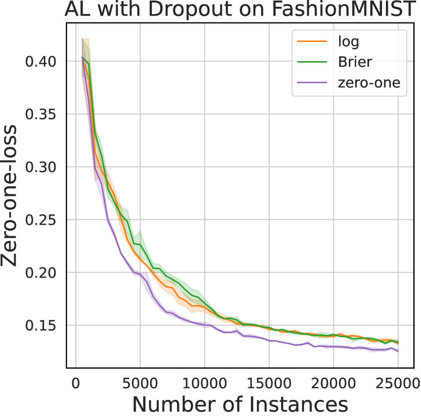
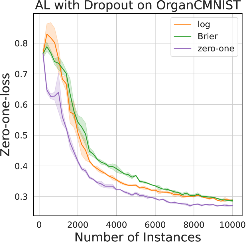
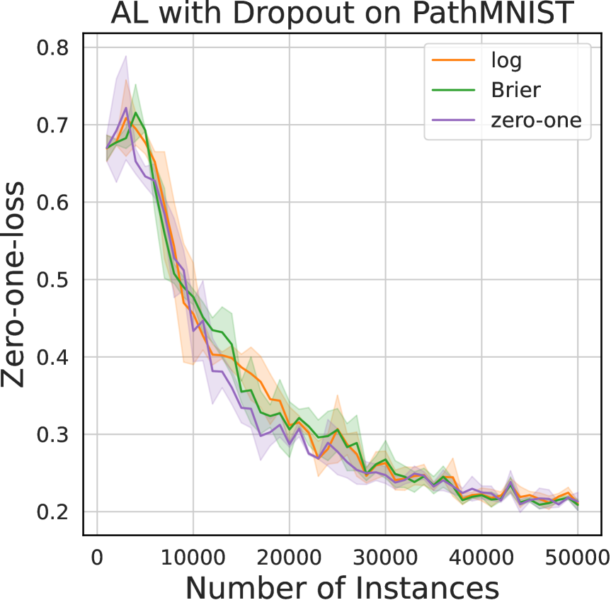
Figure 7: Active Learning with different datasets using the epistemic uncertainty component to query new instances. The model is evaluated using the zero-one-loss on the test instances. The line shows the mean and the shaded area represents the standard deviation over three runs.

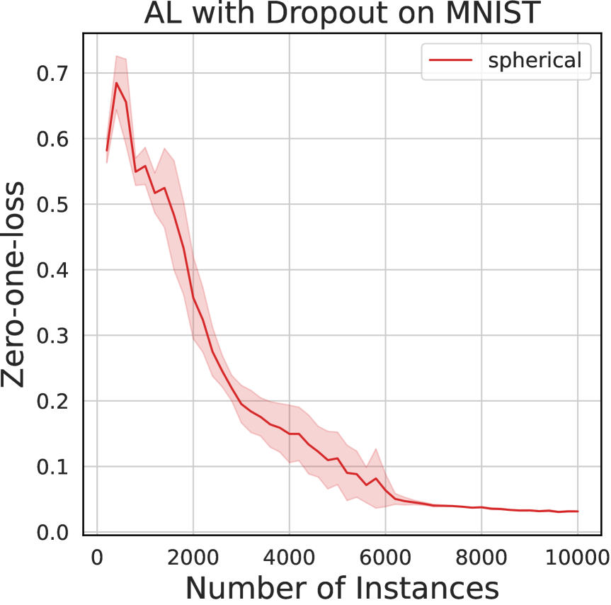
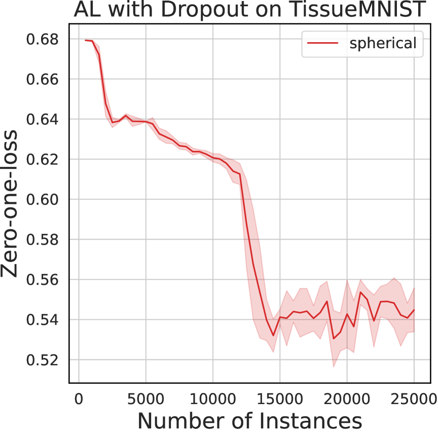
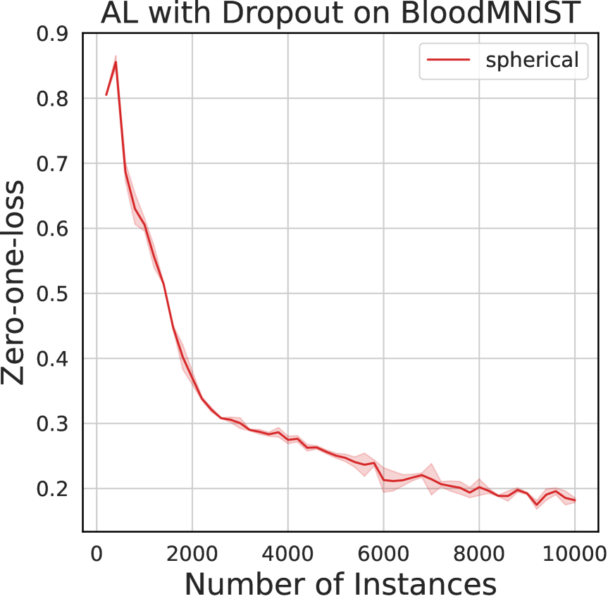
Figure 8: Active Learning with different datasets using the epistemic uncertainty component to query new instances. The model is evaluated using the zero-one-loss on the test instances. The line shows the mean and the shaded area represents the standard deviation over three runs.

References

- Amini et al. [2020] A. Amini, W. Schwarting, A. Soleimany, and D. Rus. Deep evidential regression. In H. Larochelle, M. Ranzato, R. Hadsell, M. Balcan, and H. Lin, editors, Advances in Neural Information Processing Systems 33: Annual Conference on Neural Information Processing Systems 2020, NeurIPS 2020, December 6-12, 2020, virtual, 2020.
- Banerjee et al. [2004] A. Banerjee, X. Guo, and H. Wang. Optimal bregman prediction and jensen’s equality. In Proceedings of the 2004 IEEE International Symposium on Information Theory, ISIT 2004, Chicago Downtown Marriott, Chicago, Illinois, USA, June 27 - July 2, 2004, page 169. IEEE, 2004.
- Bengs et al. [2022] V. Bengs, E. Hüllermeier, and W. Waegeman. Pitfalls of epistemic uncertainty quantification through loss minimisation. In Advances in Neural Information Processing Systems, 2022.
- Blackard [1998] J. Blackard. Covertype. UCI Machine Learning Repository, 1998. https://doi.org/10.24432/C50K5N.
- Blundell et al. [2015] C. Blundell, J. Cornebise, K. Kavukcuoglu, and D. Wierstra. Weight uncertainty in neural network. In F. R. Bach and D. M. Blei, editors, Proceedings of the 32nd International Conference on Machine Learning, ICML 2015, Lille, France, 6-11 July 2015, volume 37 of JMLR Workshop and Conference Proceedings, pages 1613–1622. JMLR.org, 2015.
- Bossard et al. [2014] L. Bossard, M. Guillaumin, and L. V. Gool. Food-101 - mining discriminative components with random forests. In D. J. Fleet, T. Pajdla, B. Schiele, and T. Tuytelaars, editors, Computer Vision - ECCV 2014 - 13th European Conference, Zurich, Switzerland, September 6-12, 2014, Proceedings, Part VI, volume 8694 of Lecture Notes in Computer Science, pages 446–461. Springer, 2014.
- Bregman [1967] L. Bregman. The relaxation method of finding the common point of convex sets and its application to the solution of problems in convex programming. USSR Computational Mathematics and Mathematical Physics, 7(3):200–217, 1967. ISSN 0041-5553.
- Brier [1950] G. W. Brier. Verification of forecasts expressed in terms of probability. Monthly Weather Review, 78(1):1–3, Jan. 1950. ISSN 1520-0493.
- Cattral and Oppacher [2006] R. Cattral and F. Oppacher. Poker hand. UCI Machine Learning Repository, dec 2006. https://doi.org/10.24432/C5KW38.
- Clarté et al. [2023] L. Clarté, B. Loureiro, F. Krzakala, and L. Zdeborová. Expectation consistency for calibration of neural networks. In R. J. Evans and I. Shpitser, editors, Uncertainty in Artificial Intelligence, UAI 2023, July 31 - 4 August 2023, Pittsburgh, PA, USA, volume 216 of Proceedings of Machine Learning Research, pages 443–453. PMLR, 2023.
- Cover and Thomas [2006] T. M. Cover and J. A. Thomas. Elements of information theory (2. ed.). Wiley, 2006. ISBN 978-0-471-24195-9.
- Daxberger et al. [2021] E. Daxberger, A. Kristiadi, A. Immer, R. Eschenhagen, M. Bauer, and P. Hennig. Laplace redux - effortless bayesian deep learning. In M. Ranzato, A. Beygelzimer, Y. N. Dauphin, P. Liang, and J. W. Vaughan, editors, Advances in Neural Information Processing Systems 34: Annual Conference on Neural Information Processing Systems 2021, NeurIPS 2021, December 6-14, 2021, virtual, pages 20089–20103, 2021.
- de Jong et al. [2024] I. P. de Jong, A. I. Sburlea, and M. Valdenegro-Toro. How disentangled are your classification uncertainties? CoRR, abs/2408.12175, 2024.
- Deng et al. [2009] J. Deng, W. Dong, R. Socher, L. Li, K. Li, and L. Fei-Fei. Imagenet: A large-scale hierarchical image database. In 2009 IEEE Computer Society Conference on Computer Vision and Pattern Recognition (CVPR 2009), 20-25 June 2009, Miami, Florida, USA, pages 248–255. IEEE Computer Society, 2009.
- Depeweg et al. [2018a] S. Depeweg, J. Hernandez-Lobato, F. Doshi-Velez, and S. Udluft. Decomposition of uncertainty in Bayesian deep learning for efficient and risk-sensitive learning. In Proc. ICML, Stockholm, Sweden, 2018a.
- Depeweg et al. [2018b] S. Depeweg, J.-M. Hernandez-Lobato, F. Doshi-Velez, and S. Udluft. Decomposition of uncertainty in bayesian deep learning for efficient and risk-sensitive learning. In International Conference on Machine Learning, pages 1184–1193. PMLR, 2018b.
- Gal and Ghahramani [2016] Y. Gal and Z. Ghahramani. Dropout as a bayesian approximation: Representing model uncertainty in deep learning. In M. Balcan and K. Q. Weinberger, editors, Proceedings of the 33nd International Conference on Machine Learning, ICML 2016, New York City, NY, USA, June 19-24, 2016, volume 48 of JMLR Workshop and Conference Proceedings, pages 1050–1059. JMLR.org, 2016.
- Gal et al. [2017] Y. Gal, R. Islam, and Z. Ghahramani. Deep bayesian active learning with image data. In D. Precup and Y. W. Teh, editors, Proceedings of the 34th International Conference on Machine Learning, ICML 2017, Sydney, NSW, Australia, 6-11 August 2017, volume 70 of Proceedings of Machine Learning Research, pages 1183–1192. PMLR, 2017.
- Geifman and El-Yaniv [2017] Y. Geifman and R. El-Yaniv. Selective classification for deep neural networks. In I. Guyon, U. von Luxburg, S. Bengio, H. M. Wallach, R. Fergus, S. V. N. Vishwanathan, and R. Garnett, editors, Advances in Neural Information Processing Systems 30: Annual Conference on Neural Information Processing Systems 2017, December 4-9, 2017, Long Beach, CA, USA, pages 4878–4887, 2017.
- Gneiting and Raftery [2005] T. Gneiting and A. Raftery. Strictly proper scoring rules, prediction, and estimation. Technical Report 463R, Department of Statistics, University of Washington, 2005.
- Gruber and Buettner [2023] S. Gruber and F. Buettner. Uncertainty estimates of predictions via a general bias-variance decomposition. In F. J. R. Ruiz, J. G. Dy, and J. van de Meent, editors, International Conference on Artificial Intelligence and Statistics, 25-27 April 2023, Palau de Congressos, Valencia, Spain, volume 206 of Proceedings of Machine Learning Research, pages 11331–11354. PMLR, 2023.
- He et al. [2016] K. He, X. Zhang, S. Ren, and J. Sun. Deep residual learning for image recognition. In 2016 IEEE Conference on Computer Vision and Pattern Recognition, CVPR 2016, Las Vegas, NV, USA, June 27-30, 2016, pages 770–778. IEEE Computer Society, 2016.
- Hendrycks and Gimpel [2017] D. Hendrycks and K. Gimpel. A baseline for detecting misclassified and out-of-distribution examples in neural networks. In 5th International Conference on Learning Representations, ICLR 2017, Toulon, France, April 24-26, 2017, Conference Track Proceedings. OpenReview.net, 2017.
- Hendrycks et al. [2021] D. Hendrycks, K. Zhao, S. Basart, J. Steinhardt, and D. Song. Natural adversarial examples. In IEEE Conference on Computer Vision and Pattern Recognition, CVPR 2021, virtual, June 19-25, 2021, pages 15262–15271. Computer Vision Foundation / IEEE, 2021.
- Hinton and van Camp [1993] G. E. Hinton and D. van Camp. Keeping the neural networks simple by minimizing the description length of the weights. In L. Pitt, editor, Proceedings of the Sixth Annual ACM Conference on Computational Learning Theory, COLT 1993, Santa Cruz, CA, USA, July 26-28, 1993, pages 5–13. ACM, 1993.
- Hüllermeier and Waegeman [2021] E. Hüllermeier and W. Waegeman. Aleatoric and epistemic uncertainty in machine learning: An introduction to concepts and methods. Machine Learning, 110(3):457–506, 2021.
- Hüllermeier et al. [2022] E. Hüllermeier, S. Destercke, and M. H. Shaker. Quantification of credal uncertainty in machine learning: A critical analysis and empirical comparison. In J. Cussens and K. Zhang, editors, Proceedings of the Thirty-Eighth Conference on Uncertainty in Artificial Intelligence, volume 180 of Proceedings of Machine Learning Research, pages 548–557. PMLR, 01–05 Aug 2022.
- Jürgens et al. [2024] M. Jürgens, N. Meinert, V. Bengs, E. Hüllermeier, and W. Waegeman. Is epistemic uncertainty faithfully represented by evidential deep learning methods? In Forty-first International Conference on Machine Learning, ICML 2024, Vienna, Austria, July 21-27, 2024. OpenReview.net, 2024.
- Kirsch et al. [2019] A. Kirsch, J. van Amersfoort, and Y. Gal. BatchBALD: Efficient and Diverse Batch Acquisition for Deep Bayesian Active Learning. In Advances in Neural Information Processing Systems, volume 32. Curran Associates, Inc., 2019.
- Kotelevskii et al. [2025] N. Kotelevskii, V. Kondratyev, M. Takáč, E. Moulines, and M. Panov. From risk to uncertainty: Generating predictive uncertainty measures via bayesian estimation. In The Thirteenth International Conference on Learning Representations, 2025.
- Krizhevsky et al. [2009] A. Krizhevsky, G. Hinton, et al. Learning multiple layers of features from tiny images. 2009.
- Kull and Flach [2015] M. Kull and P. A. Flach. Novel decompositions of proper scoring rules for classification: Score adjustment as precursor to calibration. In A. Appice, P. P. Rodrigues, V. S. Costa, C. Soares, J. Gama, and A. Jorge, editors, Machine Learning and Knowledge Discovery in Databases - European Conference, ECML PKDD 2015, Porto, Portugal, September 7-11, 2015, Proceedings, Part I, volume 9284 of Lecture Notes in Computer Science, pages 68–85. Springer, 2015.
- Lahlou et al. [2023] S. Lahlou, M. Jain, H. Nekoei, V. Butoi, P. Bertin, J. Rector-Brooks, M. Korablyov, and Y. Bengio. DEUP: direct epistemic uncertainty prediction. Trans. Mach. Learn. Res., 2023, 2023.
- Lakshminarayanan et al. [2017] B. Lakshminarayanan, A. Pritzel, and C. Blundell. Simple and scalable predictive uncertainty estimation using deep ensembles. In I. Guyon, U. von Luxburg, S. Bengio, H. M. Wallach, R. Fergus, S. V. N. Vishwanathan, and R. Garnett, editors, Advances in Neural Information Processing Systems 30: Annual Conference on Neural Information Processing Systems 2017, December 4-9, 2017, Long Beach, CA, USA, pages 6402–6413, 2017.
- LeCun et al. [1998] Y. LeCun, L. Bottou, Y. Bengio, and P. Haffner. Gradient-based learning applied to document recognition. Proc. IEEE, 86(11):2278–2324, 1998.
- Loshchilov and Hutter [2017] I. Loshchilov and F. Hutter. SGDR: stochastic gradient descent with warm restarts. In 5th International Conference on Learning Representations, ICLR 2017, Toulon, France, April 24-26, 2017, Conference Track Proceedings. OpenReview.net, 2017.
- Margraf et al. [2024] V. Margraf, M. Wever, S. Gilhuber, G. M. Tavares, T. Seidl, and E. Hüllermeier. ALPBench: A Benchmark for Active Learning Pipelines on Tabular Data, June 2024. arXiv:2406.17322 [cs].
- Minderer et al. [2021] M. Minderer, J. Djolonga, R. Romijnders, F. Hubis, X. Zhai, N. Houlsby, D. Tran, and M. Lucic. Revisiting the calibration of modern neural networks. In M. Ranzato, A. Beygelzimer, Y. N. Dauphin, P. Liang, and J. W. Vaughan, editors, Advances in Neural Information Processing Systems 34: Annual Conference on Neural Information Processing Systems 2021, NeurIPS 2021, December 6-14, 2021, virtual, pages 15682–15694, 2021.
- Mucsányi et al. [2024] B. Mucsányi, M. Kirchhof, and S. J. Oh. Benchmarking uncertainty disentanglement: Specialized uncertainties for specialized tasks. In The Thirty-eight Conference on Neural Information Processing Systems Datasets and Benchmarks Track, 2024.
- Nadeem et al. [2010] M. S. A. Nadeem, J. Zucker, and B. Hanczar. Accuracy-rejection curves (arcs) for comparing classification methods with a reject option. In S. Dzeroski, P. Geurts, and J. Rousu, editors, Proceedings of the third International Workshop on Machine Learning in Systems Biology, MLSB 2009, Ljubljana, Slovenia, September 5-6, 2009, volume 8 of JMLR Proceedings, pages 65–81. JMLR.org, 2010.
- Netzer et al. [2011] Y. Netzer, T. Wang, A. Coates, A. Bissacco, B. Wu, and A. Y. Ng. Reading digits in natural images with unsupervised feature learning. In NIPS Workshop on Deep Learning and Unsupervised Feature Learning 2011, 2011.
- Nguyen et al. [2019] V.-L. Nguyen, S. Destercke, and E. Hüllermeier. Epistemic Uncertainty Sampling. In P. Kralj Novak, T. Šmuc, and S. Džeroski, editors, Discovery Science, pages 72–86, Cham, 2019. Springer International Publishing. ISBN 978-3-030-33778-0.
- Pandey and Yu [2023] D. S. Pandey and Q. Yu. Learn to accumulate evidence from all training samples: Theory and practice. In A. Krause, E. Brunskill, K. Cho, B. Engelhardt, S. Sabato, and J. Scarlett, editors, International Conference on Machine Learning, ICML 2023, 23-29 July 2023, Honolulu, Hawaii, USA, volume 202 of Proceedings of Machine Learning Research, pages 26963–26989. PMLR, 2023.
- Paszke et al. [2019] A. Paszke, S. Gross, F. Massa, A. Lerer, J. Bradbury, G. Chanan, T. Killeen, Z. Lin, N. Gimelshein, L. Antiga, A. Desmaison, A. Köpf, E. Z. Yang, Z. DeVito, M. Raison, A. Tejani, S. Chilamkurthy, B. Steiner, L. Fang, J. Bai, and S. Chintala. Pytorch: An imperative style, high-performance deep learning library. In H. M. Wallach, H. Larochelle, A. Beygelzimer, F. d’Alché-Buc, E. B. Fox, and R. Garnett, editors, Advances in Neural Information Processing Systems 32: Annual Conference on Neural Information Processing Systems 2019, NeurIPS 2019, December 8-14, 2019, Vancouver, BC, Canada, pages 8024–8035, 2019.
- Pedregosa et al. [2011] F. Pedregosa, G. Varoquaux, A. Gramfort, V. Michel, B. Thirion, O. Grisel, M. Blondel, P. Prettenhofer, R. Weiss, V. Dubourg, J. Vanderplas, A. Passos, D. Cournapeau, M. Brucher, M. Perrot, and E. Duchesnay. Scikit-learn: Machine learning in Python. Journal of Machine Learning Research, 12:2825–2830, 2011.
- Ridnik et al. [2021] T. Ridnik, E. B. Baruch, A. Noy, and L. Zelnik. Imagenet-21k pretraining for the masses. In J. Vanschoren and S. Yeung, editors, Proceedings of the Neural Information Processing Systems Track on Datasets and Benchmarks 1, NeurIPS Datasets and Benchmarks 2021, December 2021, virtual, 2021.
- Sale et al. [2023] Y. Sale, V. Bengs, M. Caprio, and E. Hüllermeier. Second-order uncertainty quantification: A distance-based approach. arXiv preprint arXiv:2312.00995, 2023.
- Sale et al. [2024] Y. Sale, P. Hofman, T. Löhr, L. Wimmer, T. Nagler, and E. Hüllermeier. Label-wise aleatoric and epistemic uncertainty quantification. In The 40th Conference on Uncertainty in Artificial Intelligence, 2024.
- Savage [1971] L. J. Savage. Elicitation of personal probabilities and expectations. Journal of the American Statistical Association, 66(336):783–801, 1971.
- Schweighofer et al. [2024] K. Schweighofer, L. Aichberger, M. Ielanskyi, and S. Hochreiter. On Information-Theoretic Measures of Predictive Uncertainty, Oct. 2024. arXiv:2410.10786.
- Sensoy et al. [2018] M. Sensoy, L. Kaplan, and M. Kandemir. Evidential deep learning to quantify classification uncertainty. In Proc. NeurIPS, 32nd Conference on Neural Information Processing Systems, Montreal, Canada, 2018.
- Smith et al. [2024] F. B. Smith, J. Kossen, E. Trollope, M. van der Wilk, A. Foster, and T. Rainforth. Rethinking aleatoric and epistemic uncertainty. In NeurIPS 2024 Workshop on Bayesian Decision-making and Uncertainty, 2024.
- Smith and Gal [2018] L. Smith and Y. Gal. Understanding measures of uncertainty for adversarial example detection. In A. Globerson and R. Silva, editors, Proceedings of the Thirty-Fourth Conference on Uncertainty in Artificial Intelligence, UAI 2018, Monterey, California, USA, August 6-10, 2018, pages 560–569. AUAI Press, 2018.
- Wimmer et al. [2023] L. Wimmer, Y. Sale, P. Hofman, B. Bischl, and E. Hüllermeier. Quantifying aleatoric and epistemic uncertainty in machine learning: Are conditional entropy and mutual information appropriate measures?, 2023.
- Xiao et al. [2017] H. Xiao, K. Rasul, and R. Vollgraf. Fashion-mnist: a novel image dataset for benchmarking machine learning algorithms. arXiv preprint arXiv:1708.07747, 2017.
- Yang et al. [2023] J. Yang, R. Shi, D. Wei, Z. Liu, L. Zhao, B. Ke, H. Pfister, and B. Ni. Medmnist v2-a large-scale lightweight benchmark for 2d and 3d biomedical image classification. Scientific Data, 10(1):41, 2023.
- Zhou et al. [2018] B. Zhou, À. Lapedriza, A. Khosla, A. Oliva, and A. Torralba. Places: A 10 million image database for scene recognition. IEEE Trans. Pattern Anal. Mach. Intell., 40(6):1452–1464, 2018.