Quantum engineering of high harmonic generation

Abstract

In quantum sideband high harmonic generation (QSHHG), high harmonic generation is perturbed by a bright quantum field resulting in harmonic sidebands, with the intent to transfer non-classical properties from the quantum perturbation to the harmonic sidebands. So far, non-classical features have not been found in QSHHG yet. The closed form theory of QSHHG in atoms and solids developed here answers the question under which conditions non-classical features can be realized. QSHHG results in a multi-mode entanglement between harmonic sideband modes and perturbative quantum mode. A projective measurement on either creates a variety of non-classical states commonly used in quantum information science. This opens a pathway towards quantum engineering high harmonic generation as a short wavelength source for quantum information science.

I Introduction

High harmonic generation (HHG) is a coherent source for XUV (extreme ultraviolet) generation and presents the key process for many spectroscopic applications in attosecond science [1]. It is successfully described within the semi-classical approximation, whereby the atomic dynamics are described quantum mechanically in conjunction with a classical model of the electromagnetic field [2]. This approach allows a simple interpretation of HHG in terms of a three-step process, consisting of ionization, free electron quiver excursion driven by the laser field, and emission of high harmonic radiation during recombination with the parent ion [3]. Over the past few decades, significant progress in understanding and utilization of HHG in both gaseous and solid media has been made possible via the use of the semi-classical approximation [4, 5].

Only recently has HHG been analyzed from a quantum optical perspective. By describing the harmonic emission process with quantum optical operators and modeling the intense laser field classically, it has been demonstrated that the photon statistics of high harmonic (HH) radiation can be modified under certain conditions [6, 7], such as by accounting for the electron dynamics between bound states. HHG has also been described in two-level atoms using quantum optical models [8, 9] and has been shown both theoretically and experimentally to induce non-classical Schrödinger cat states in the intense laser modes [10, 11, 12, 13]. Additional intriguing predictions from theory include light-electron entanglement during above threshold ionization [14], entangled x-ray photon pair generation through HHG from pair production [15], and entanglement between harmonics in intense laser driven atoms, when a resonance lies close to a harmonic [16]. In the limit of strong field driving, when the atomic ground state gets depleted, the quantum state of the driving field and harmonics become entangled and squeezed [17].

Furthermore, theoretical and experimental investigations have started to look into the modification of strong field physics in the case where the intense laser field is replaced by a bright squeezed vacuum (BSV) beam. Full quantum optical calculations have predicted substantial deviations from the semi-classical three-step model, the most notable of which are harmonics beyond the semi-classical cutoff, higher damage thresholds, and the photon statistics of the BSV influencing the emitted electrons [18, 19, 20, 21].

Developing quantum sources at shorter wavelengths is a desirable goal, because of the higher information density and lower noise of detectors. The required intensity for extending HHG into the XUV (extreme ultraviolet) range presents a challenge, if the only driving field is intended to be quantum mechanical. Ideally, for applications in quantum information science [14] one desires a coherent process that can be scaled to the XUV, in which quantum properties can be engineered at will. These have been the guiding principles behind a recent experiment: perturbing regular HHG with a BSV to produce quantum sideband high harmonics (QSHH) that exhibit super-Poissonian photon-bunching statistics [22].

The goal of this work is to develop the theory of quantum sideband high harmonic generation (QSHHG) in atoms and solids and to identify methods by which to transfer quantum properties from the perturbative BSV onto the harmonic sidebands. The theoretical framework is a quantum generalization of the semi-classical Lewenstein model of HHG [2] and yields closed-form solutions for the HHG and QSHHG wavefunctions. Knowledge of the wavefunction enables identification of the quantum properties of QSHHG. The additional photons absorbed and emitted from the quantum perturbation, such as a BSV, create entanglement between individual harmonic sidebands and between the harmonic sidebands and the BSV. We show how this entanglement can be harnessed to create a variety of non-classical states commonly used in quantum information science, such as high purity single photon states, Schrödinger cat states, and photon added squeezed vacuum states. In this way, quantum properties of the BSV can be transferred onto QSHHG, opening a path towards engineering the quantum properties of ultrashort XUV high harmonics. While we primarily focus on single-mode properties, a qualitative discussion of two- and multi-mode entanglement is given in the following text. A more quantitative analysis is subject to future research.

In addition to revealing quantum properties of QSHHG, the theory offers an order of magnitude predictive power regarding the number of photons in the harmonics and sidebands and compares very favorably with experiments [22]. This facilitates the optimization of QSHHG, thereby relaxing the requirements on the BSV power.

II Theory summary

We use a strong field quantum optical model that generalizes the semi-classical approach of Lewenstein [3, 2]. Although the derivation is quite general, results and conclusions are derived for a BSV quantum perturbation at twice the frequency of the classical driving field which results in even harmonic sidebands. For a detailed derivation see the supplement [23]. In the quantum optical description, HHG is modeled as a one photon process: $N$ classical photons are emitted as a single high harmonic (HH) photon. QSHHG is, to lowest order, a two-photon process, wherein the emission of a harmonic photon is perturbed by the emission or absorption of a quantum photon, resulting in the effective emission of a QSHH photon. The international system of (SI) units is used, unless otherwise noted.

II.1 Wavefunction

HHG and QSHHG are described by the photon wavefunction

$$\left|\varphi_{0}(t)\right\rangle\!\approx\!\left|\varphi_{h}(t)\right\rangle\left|\varphi_{m}(t)\right\rangle\!=\!\hat{D}_{h}\hat{S}_{m}\left|\varphi_{0}(t_{0})\right\rangle\mathrm{}$$ (1)

with $|\varphi_{0}(t_{0})\rangle$ the wavefunction at initial time $t_{0}$. We assume that HHG and QSHHG take place in different modes $\kappa$. The wavefunction can therefore be written as an independent product of these two processes. For example, coupling between QSHHG and HHG occurs for three-photon processes, when the frequency of the perturbing quantum field is twice that of the classical one [24, 25]. It can also occur in a first order process when the perturbing and driving fields have the same frequency. Both cases are subject to future research. A generalization of our approach is outlined in the supplement [23]. HHG and QSHHG are determined in the limit $\left|\varphi_{h,m}\right\rangle=\left|\varphi_{h,m}(t\rightarrow\infty)\right\rangle$.

The HHG wavefunction $\left|\varphi_{h}\right\rangle$ is generated by the displacement operator

$$\hat{D}_{h}=\exp\left(\sum_{\kappa}h_{\kappa}\hat{a}^{\dagger}_{\kappa}-h^{*}_{\kappa}\hat{a}_{\kappa}\right)\mathrm{,}$$ (2)

where $\kappa\equiv(\mathbf{k}s)$ is a multi-index with photon wavevector $\mathbf{k}$, polarization index $s=1,2$. The HHG coefficient $h_{\kappa}$ is defined in the next section; it contains a sum over an ensemble of emitters at positions $\mathbf{x}_{j}$. The position dependence is not written explicitly.

The QSHHG wavefunction $\left|\varphi_{m}(t)\right\rangle$ is generated by a mixed-mode squeezed vacuum state operator between harmonic modes $\kappa$ and perturbative quantum modes $q$,

$$\hat{S}_{m}=\exp\left(\sum_{\kappa}\left(f_{\kappa}\hat{a}^{\dagger}_{q}+g_{\kappa}\hat{a}_{q}\right)\hat{a}^{\dagger}_{\kappa}-\left(g^{*}_{\kappa}\hat{a}^{\dagger}_{q}+f^{*}_{\kappa}\hat{a}_{q}\right)\hat{a}_{\kappa}\right)\mathrm{.}$$ (3)

Our analysis is confined to a single perturbative mode $q$. The coefficients $f_{\kappa},g_{\kappa}$ represent HHG in the presence of emission and absorption of an additional perturbative quantum photon, respectively. In perturbative nonlinear optics, the former is referred to as difference (DFG) and the latter as sum frequency (SFG) generation. QSHHG coefficients $f_{\kappa},g_{\kappa}$ are defined in the next subsection.

In order to fully define Eq. (1), a particular initial state needs to be chosen; $|\varphi_{0}(t_{0})\rangle=|v\xi_{q}\rangle$ consists of a multi-mode vacuum state, $|v\rangle=\prod_{\kappa}|v_{\kappa}\rangle$, for the harmonics, and a single squeezed vacuum state for the perturbative mode,

$$\left|\xi_{q}\right\rangle=\hat{S}_{q}\left|v_{q}\right\rangle=e^{\frac{1}{2}(\xi\hat{a}_{q}^{2}-\xi^{*}\hat{a}_{q}^{\dagger 2})}\left|v_{q}\right\rangle$$ (4)

with $\xi=re^{i\theta}$. Normal ordering of $\left|\varphi_{m}\right\rangle\!=\!\hat{S}_{m}\left|v\xi_{q}\right\rangle$ yields [23] with $\beta=(1/2)\tanh(r)e^{-i\theta}$, and $\overline{\beta}=\beta/(1+\sum_{\kappa}|Z_{\kappa}|^{2})$. Further,

$$Z_{\kappa} =f_{\kappa}-g_{\kappa}\tanh(r)e^{i\theta}$$

$$\overline{\frak{N}} =\frac{1}{\sqrt{1+\sum_{\kappa}|Z_{\kappa}|^{2}}}\mathrm{.}$$ (5)

Equation (LABEL:nord) is a multi-mode harmonics wavefunction in the basis of electromagnetic plane wave modes, and can be used to calculate two or more correlated mode properties. The normal-ordered wavefunction has been derived in the limit of an intense squeezed vacuum beam with $r>1$ and $|Z_{\kappa}|^{2}\ll 1$.

II.2 HHG and QSHHG coefficients for atomic and molecular gases

The HHG coefficient of a single atom $j$ is given by [23]

$$h_{\kappa} =-e^{-i\mathbf{k}\mathbf{x}_{j}}\!\!\int_{-\infty}^{\infty}\!\!\!\!dte^{i\omega_{k}t}H_{k}(t)=\tilde{H}_{k}e^{-i\mathbf{k}\mathbf{x}_{j}}$$ (6)

$$H_{k} =\frac{|e|E_{v}}{\hbar}\Biggl{\{}\mathbf{e}_{\kappa}\mathbf{x}(t)+\int\!\!d^{3}\mkern-2.0mup\,\overline{\sigma}_{\kappa}(t)\left(\Gamma_{\mathbf{p}}(t)+\mathrm{c.c}\right)\Biggr{\}}\mathrm{}$$

with

$$\mathbf{x}(t)=\int\!\!d^{3}\mkern-2.0mup\,\mathbf{d}^{*}\!(\mathbf{p}_{t})\,b_{\mathbf{p}}(t)+\mathrm{c.c.}$$ (7)

$$b_{\mathbf{p}}(t)=\int_{t_{0}}^{t}dt^{\prime}\,\Omega(t^{\prime})\exp\left(iS(t^{\prime},t)-\xi(t-t^{\prime})\right)\mathrm{.}$$

The polarization of HHG is assumed to be parallel to the laser pulse; additionally, $H_{k}$ does not depend on the direction of the wavevector. Both facts are reflected in the change of the lower index from $\kappa$ to $k=\omega_{k}/c$. Note that $H_{k}$ depends on the position $\mathbf{x}_{j}$ of the atom via the space dependence of the laser field, which is not explicitly stated. Frequency and polarization of the harmonic are given by $\omega_{k}$ and $\mathbf{e}_{\boldsymbol{\kappa}}$, $\mathbf{d}(\mathbf{p})=\langle\mathbf{p}|\mathbf{x}|0\rangle=d_{0}\mathbf{p}/(\mathbf{p}^{2}/(2m)+E_{0})^{3}$ is the transition dipole moment between ground $|0\rangle$ and continuum plane wave state $|\mathbf{p}\rangle$ with $\mathbf{p}$ in the canonical momentum frame [2], $E_{0}$ is the binding energy, and $d_{0}=3.37\times 10^{-4}\,[\mathrm{kg^{1/2}m^{9/2}s^{-7/2}}]$. Further, $\Omega(t)=(|e|/\hbar)\mathbf{d}(\mathbf{p}_{t})\boldsymbol{\mathcal{F}}(t)$ is a generalized Rabi frequency, $\boldsymbol{\mathcal{F}}$ represents the classical intense laser field, $\mathbf{p}_{\mkern-1.5mut}=\mathbf{p}+|e|\boldsymbol{\mathcal{A}}(t)$ is defined in the moving momentum frame, and $-\partial_{t}\boldsymbol{\mathcal{A}}(t)=\boldsymbol{\mathcal{F}}(t)$ defines the vector potential. Note that the electric field consists of a classical part $\boldsymbol{\mathcal{F}}$ with frequency $\omega_{0}$ and field strength $F_{0}$, and of a quantum part $\hat{\mathbf{F}}$ which accounts for the emission of harmonic photons in Eqs. (2) and (3). Moreover, $E_{v}=\sqrt{\hbar\omega_{k}/2\varepsilon_{0}V}$ is the vacuum electric field, $V$ the quantization volume, and $\varepsilon_{0}$ the vacuum permittivity. We use a filter $\xi(t-t^{\prime})$ that leaves HHG from the first recollision unchanged and extinguishes all higher returns [23]. The dipole $\mathbf{x}(t)$ corresponds with the semiclassical Lewenstein dipole defined in Eq. (6) of Ref. [2] with

$$S(t)=\frac{1}{\hbar}\int_{t_{0}}^{t}\!\left(\frac{1}{2m}\mathbf{p}^{2}_{\mkern-1.5mu\tau}+E_{0}\right)d\tau\mathrm{}$$ (8)

the classical action, and $S(t^{\prime},t)=S(t)-S(t^{\prime})$. Further,

$$\Gamma_{\mathbf{p}}(t)=\Omega^{*}(t)b_{\mathbf{p}}(t)$$ (9)

is related to the optical field ionization rate $2\mathrm{Re}[\gamma]$ with $\gamma(t)=\int d^{3}\mkern-1.5mup\,\Gamma_{\!\mathbf{p}}(t)$, see Eq. (52) of [2]. Finally, during ionization an electron is promoted into a laser driven continuum state, dressed with a displacement operator [23] with coefficient

$$\sigma_{\kappa}(t)=\!\frac{|e|E_{v}}{\hbar}\overline{\sigma}_{\kappa}(t)e^{i\omega_{k}t}$$

$$\overline{\sigma}_{\kappa}(t)=\!-\frac{i}{\omega_{k}}\!\int_{t_{0}}^{t}dt^{\prime}\left(\mathbf{e}_{\kappa}\mathbf{v}_{t^{\prime}}\right)e^{-i\omega_{k}(t-t^{\prime})}\mathrm{.}$$ (10)

Here, $\mathbf{v}=\mathbf{p}/m$ is the electron velocity. HHG, as described by $H_{k}$ in Eq. (6), contains two contributions. The first term represents HHG via ionization, continuum evolution, and recollision [3, 2]. The second term describes HHG via the ionization nonlinearity [26].

The QSHHG coefficients $f_{\kappa},g_{\kappa}$ for a single atom $j$ are given by

$$f_{\kappa} \!=\!e^{-i(\mathbf{k}+\mathbf{q})\mathbf{x}_{j}}\!\!\!\int_{-\infty}^{\infty}\!\!\!\!\!dte^{i(\omega_{k}+\omega_{q})t}F_{k}(t)\!=\!\tilde{F}_{k}e^{-i(\mathbf{k}+\mathbf{q})\mathbf{x}_{j}}$$

$$F_{k} \!=\!\left(\!\frac{|e|E_{v}}{\hbar}\!\right)^{\!2}\!\!\!\int\!\!d^{3}\mkern-2.0mup\,\overline{\sigma}_{q}(t)\biggl{\{}\mathbf{e}_{\kappa}\mathbf{x}_{\mathbf{p}}(t)\!+\!i\overline{\sigma}_{\kappa}(t)\mathrm{Im}\left[\Gamma_{\mathbf{p}}(t)\right]\biggr{\}}$$ (11)

and

$$g_{\kappa} \!=\!e^{-i(\mathbf{k}-\mathbf{q})\mathbf{x}_{j}}\!\!\!\int_{-\infty}^{\infty}\!\!\!\!\!dte^{i(\omega_{k}-\omega_{q})t}G_{k}(t)\!=\!\tilde{G}_{k}e^{-i(\mathbf{k}-\mathbf{q})\mathbf{x}_{j}}$$

$$G_{k} \!=\!\left(\!\frac{|e|E_{v}}{\hbar}\!\right)^{\!2}\!\!\!\int\!\!d^{3}\mkern-2.0mup\,\overline{\sigma}^{*}_{q}(t)\biggl{\{}\mathbf{e}_{\kappa}\mathbf{x}_{\mathbf{p}}(t)\!+\!i\overline{\sigma}_{\kappa}(t)\mathrm{Im}\left[\Gamma_{\mathbf{p}}(t)\right]\biggr{\}}\mathrm{,}$$ (12)

where $\omega_{q}$ and $\mathbf{q}$ are frequency and wavevector of the quantum light mode $q$, and

$$\mathbf{x}_{\mathbf{p}}(t)=\mathbf{d}^{*}\!(\mathbf{p}_{t})\,b_{\mathbf{p}}(t)-\mathrm{c.c.}$$ (13)

is the imaginary part of the transition dipole for a given $\mathbf{p}$. Again, the index of $F,G$ has been changed from $\kappa$ to $k$. Both, conventional HHG and QSHHG coefficients are very similar to the semi-classical coefficients [25], except for powers of the quantum vacuum field term $|e|E_{v}/\hbar$. In the quasi-classical approach the coefficient $\overline{\sigma}_{q}(t)$ is within the time integral of $\mathbf{x}_{\mathbf{p}}(t)$. The same is initially the case for the quantum optical equations. However, in order to obtain a unitary QSHHG operator, $\overline{\sigma}_{q}$ needs to be pulled out of the inner time integral by integration by parts. The remaining non-unitary term is small and can be neglected, see the discussion between Eqs. (S14) and (S15) in section I.A of the supplement [23].

II.3 HHG and QSHHG coefficients for solids

The results for atomic and molecular gases can be easily translated into HHG in two-band solids by replacing

$$\mathbf{p}\rightarrow\mathbf{k},\,\,\,\,\mathbf{k}\in\mathrm{BZ}$$ (14a)

$$E_{0}+\frac{\mathbf{p}^{2}}{2m}\rightarrow\varepsilon(\mathbf{k})\approx E_{g}+\frac{\mathbf{p}^{2}}{2m_{*}}=\varepsilon(\mathbf{p})$$ (14b)

$$\frac{\mathbf{p}}{m}\rightarrow\frac{1}{\hbar}\nabla_{\mathbf{k}}\varepsilon=\mathbf{v}(\mathbf{k})\approx\frac{\mathbf{p}}{m_{*}}$$ (14c)

$$\mathbf{d}(\mathbf{p})\rightarrow\mathbf{d}(\mathbf{k})=-i\langle u_{c}(\mathbf{k})|\nabla_{\mathbf{k}}|u_{v}(\mathbf{k})\rangle\approx\frac{d_{0}E_{g}}{\varepsilon(\mathbf{p})}$$ (14d)

where $\mathbf{k}$ represents the crystal momentum defined in the first Brillouin zone (BZ), and $\varepsilon(\mathbf{k})$ and $\mathbf{v}(\mathbf{k})$ represent relative band gap and band velocity, i.e. the difference between conduction and valence bands. The minimum band gap is $E_{g}=E_{0}$, $m_{*}$ is the effective electron mass at the band gap minimum defined by $\partial_{k_{i}}\partial_{k_{j}}\varepsilon|_{\mathbf{k}=0}=\hbar^{2}/m_{*}$. For simplicity, we have replaced the inverse effective mass tensor by a scalar quantity. Finally, the atomic transition dipole needs to be replaced with the dipole moment between valence and conduction bands. The last term is the approximate dipole moment in $\mathbf{k}\mathbf{p}$ perturbation theory [27]. Within the effective mass approximation, the atomic equations remain applicable to solids and are represented by the last terms in Eqs. (14a)-(14d).

II.4 Phase matching

In order to compare and characterize HHG and QSHHG, operator expectation values with regard to the macroscopic wavefunction need to be known. Here, we focus on $\hat{n}=\sum_{\kappa}\hat{n}_{\kappa}$,

$$\langle\varphi_{h}|\hat{n}|\varphi_{h}\rangle=\sum_{\kappa}\!\left(\sum_{j}h^{*}_{\kappa}\right)\!\!\left(\sum_{j}h_{\kappa}\right)$$

$$=\frac{VN_{0}^{2}}{(2\pi)^{3}}\!\int\!\!d^{3}\mkern-1.5muk\left(\int\!\!d^{3}\mkern-1.5mux\,h^{*}_{\kappa}\!\right)\left(\int\!\!d^{3}\mkern-1.5mux\,h_{\kappa}\!\right)\mathrm{.}$$ (15)

In the continuum limit, the sum over atoms $\sum_{i}\rightarrow N_{0}\int d^{3}\mkern-1.5mux$, with $N_{0}$ representing the number density of the material and $\sum_{\kappa}\rightarrow V/(2\pi)^{3}\int d^{3}\mkern-1.5muk$, with $V$ as the quantization volume. Polarization and wavevector of intense laser, quantum field, HHG, and QSHHG are fixed along $x$ and $z$, respectively. The space integrals and the transverse $k_{x}$- and $k_{y}$-integrals can be worked out approximately (see [23]). At this point, the only remaining integral is the one over $dk_{z}\approx dk=d\omega_{k}/c$. The $d\omega_{k}$ integral drops out upon examination of the differential expectation value of the number operator,

$$\frac{d\langle\hat{n}\rangle}{d\omega_{k}} =\frac{d}{d\omega_{k}}\langle\varphi_{h}|\hat{n}|\varphi_{h}\rangle=c_{k}^{2}\,|\tilde{H}_{k}(\omega_{k})|^{2}$$

$$c_{k}^{2} =\frac{\left(N_{0}\mathrm{w}_{k}l_{i}\right)^{2}}{2c}V\mathrm{,}$$ (16)

where $\mathrm{w}_{k}=\mathrm{w}(\omega_{k})$ represents the transverse $1/e^{2}$ radius of the HH mode with frequency $\omega_{k}$. Here, $\tilde{H}_{k}=\tilde{H}_{k}(\mathbf{x}=0)$, since the space dependence has been integrated over, and the interaction length is $l_{i}$. HHG scales as $l_{i}^{2}$, as long as $l_{i}$ is shorter than the dephasing length. Finally, the quantization volume cancels out due to the fact that the single atom response $\tilde{H}_{k}\propto 1/\sqrt{V}$.

We are mainly interested in the number of photons emitted in all spatial modes with frequencies in the band $(N-\frac{1}{2})\omega_{0}\leq\omega_{k}\leq(N+\frac{1}{2})\omega_{0}$ which is given by

$$\langle\hat{n}\rangle_{\!N}=c_{k}^{2}\int_{(N-\frac{1}{2})\omega_{0}}^{(N+\frac{1}{2})\omega_{0}}\!\!\!\!d\omega_{k}|\tilde{H}_{k}(\omega_{k})|^{2}=|h_{N}|^{2}\mathrm{,}$$ (17)

with $h_{N}$ being a dimensionless quantity.

Similarly, the number of QSHHG photons emitted into one harmonic interval $\omega_{0}$ about harmonic order $N$ is found to be [23]

$$\langle\hat{n}\rangle_{\!N}\!=\!c_{q}^{2}\cosh^{2}(r)\int_{(N-\frac{1}{2})\omega_{0}}^{(N+\frac{1}{2})\omega_{0}}\!\!\!\!d\omega_{k}\left|\zeta_{k}\right|^{2}=\cosh^{2}(r)\left|\zeta_{N}\right|^{2}\mathrm{}$$ (18)

with

$$|\zeta_{k}|^{2}=\left|\tilde{F}_{k}-\tilde{G}_{k}\tanh(r)e^{i\theta}\right|^{2}\mathrm{,}$$

$$c_{q}^{2}=\frac{\left(N_{0}\mathrm{w}_{k}l_{i}\right)^{2}}{2c}V^{2}\frac{(\Delta q)^{3}}{(2\pi)^{3}}\mathrm{,}$$ (19)

and $(\Delta q)^{3}$ is the mode volume of the perturbative quantum field. It should be noted that we have approximated the temporally and spatially finite BSV field by a plane wave. This is being corrected for by replacing the plane wave mode volume by the experimentally measured BSV mode volume [22]. The parameter $\zeta_{k}$ emerges from $Z_{\kappa}$ in Eq. (5) after performing the phase matching integrals [23]. The quantization volume again drops out. Similar to the case for HHG, $\zeta_{N}=\zeta_{N}(\mathbf{x}=0)$.

II.5 Effective QSHH mode

In experiments [22], the photons contained in one QSHH are measured and not in the individual plane wave modes. To that end, the connection between calculations and experiment is greatly facilitated by introducing an effective mode operator [28]

$$\hat{a}_{N}=\frac{1}{|\zeta_{N}|}\sum_{\kappa\in N}Z^{*}_{\kappa}\hat{a}_{\kappa}$$ (20)

that encompasses all plane wave modes of a quantum sideband. This operator fulfills the usual harmonic oscillator commutation relations $[\hat{a}_{N},\hat{a}^{\dagger}_{M}]=\delta_{NM}$. The vacuum state of a QSHH mode is $\prod_{\kappa\in N}|v_{\kappa}\rangle=|v\rangle_{N}$, so that a number state

$$|n\rangle_{N}=\frac{1}{\sqrt{n!}}\left(\hat{a}_{N}^{\dagger}\right)^{n}|v_{N}\rangle\mathrm{,}$$ (21)

corresponds to a sum over all combinations that have $n$ photons in the plane wave modes of the quantum sideband $N$. With these definitions the wavefunction (LABEL:nord) becomes

$$\left|\varphi_{m}\right\rangle\!=\!\prod_{N}\frac{\frak{N}_{N}}{\sqrt{\cosh(r)}}\exp\!\left(|\zeta_{N}|\hat{a}_{N}^{\dagger}\hat{a}_{q}^{\dagger}\right)\exp\!\left(-\beta_{N}\hat{a}_{q}^{\dagger 2}\right)\left|v_{N}v_{q}\right\rangle\mathrm{,}$$

$$\beta_{N}=\frac{\beta}{1+\sum_{\kappa\in N}|Z_{\kappa}|^{2}}=\frac{\beta}{1+|\zeta_{N}|^{2}}\mathrm{,}$$

$$\frak{N}_{N}=\frac{1}{\sqrt{1+\sum_{\kappa\in N}|Z_{\kappa}|^{2}}}=\frac{1}{\sqrt{1+|\zeta_{N}|^{2}}}\mathrm{.}$$ (22)

This wavefunction will be used throughout the remaining text.

III Results

The following section begins with the calculation of the macroscopic photon numbers emitted by HHG and QSHHG and an associated discussion. This is followed by plotting the two-mode distribution function, which resembles a two-mode squeezed state and is entangled. Some entanglement features are briefly discussed. The rest of the paper focuses mainly on single-mode properties. From the two-mode distribution function, the QSHHG distribution function is calculated. This reveals why the non-classical properties of the BSV perturbation are not carried over onto the QSHH state. Finally, projective measurements are discussed, where the photon number of the QSHH ($N$) or perturbative ($q$) mode is measured, resulting in a wavefunction in the other mode which carries interesting non-classical properties, such as squeezing and a Wigner function with negative values.

III.1 QSHHG: gases versus solids

In Fig. ​1 QSHHG in solids (a-c) and in atoms (d) is compared. We utilize Eq. (14) to model the ZnO band structure. The parameters used are $m_{*}\approx 0.25m$, $E_{g}=3.4$ eV, and $d_{0}\!=\!7\times 10^{25}\,\left[\mathrm{{s^{2}/(kg^{3}\cdot m)}}\right]^{1/2}$, the last of which is converted from $d_{0}\!=\!4$ atomic units in Ref. [27]. The laser parameters are those which were used in recent experiments [22]: wavelength $\lambda_{0}=3.2$ µm and peak electric field strength $F_{0}=1.3\times 10^{9}$ V/m, corresponding to peak intensity $I_{0}=5\times 10^{11}$ W/cm². The electric field consists of a sine-carrier and a Gaussian envelope with pulse durations $\tau=6T_{0}$, where oscillation period $T_{0}=2\pi/\omega_{0}\approx 10$fs. The macroscopic propagation parameters are $N_{0}=4\times 10^{22}$ cm^-3, $\mathrm{w}_{k}=40$ µm (assumed to be approximately half of the laser beam width due to the HHG nonlinearity), and $l_{i}=5$ nm as determined by the absorption length. This results in the macroscopic HHG factor $(N_{0}\mathrm{w}_{k}l_{i})^{2}/(2c)\approx 10^{23}$ s/m³; $\omega_{q}=2\omega_{0}$ is used for the squeezed vacuum field. From the pulse energy of $10$ nJ, [22] one obtains $r=13.6$ and $\sinh^{2}(r)\approx\cosh^{2}(r)=10^{11}$ via the relation $\hbar\omega_{q}\langle\hat{n}_{q}\rangle=\hbar\omega_{q}\sinh^{2}r=10^{-8}$ J. The mode volume of the perturbative quantum beam must also be known for macroscopic QSHHG . In accordance with experiments [22], we choose a transverse width $\mathrm{w}_{q}=100$ µm and bandwidth $\Delta\lambda_{q}=50$ nm. Inserting these values into the expression for the mode volume gives $(2\pi/\Delta q)^{3}=(2\pi)^{3}\Delta\lambda_{q}/(\mathrm{w}_{q}\lambda_{q})^{2}=2\times 10^{12}$ m³.

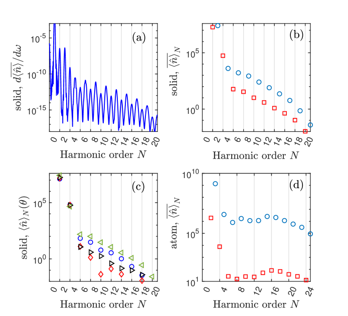
Figure 1: (a-c) HHG (odd) and QSHHG (even) spectrum in ZnO versus harmonic order N; (a) differential number of HH photons $d\overline{\langle\hat{n}\rangle}/d\omega$; (b) number of photons in the effective mode $\overline{\langle\hat{n}\rangle}_{N}$; HHG (blue circles), QSHHG (red circles). (a)-(b) average over squeezed vacuum phase $\theta$. (c) $\langle\hat{n}\rangle_{N}(\theta)$: blue circles, red diamonds, black right-pointing triangles, green left-pointing triangles correspond to $\theta=0,\pi/4,3\pi/8,7\pi/4$, respectively. (d) $\overline{\langle\hat{n}\rangle}_{N}$ averaged over $\theta$ for an atomic gas; HHG (blue circles), QSHHG (red squares). For parameters see text.

The atomic gas parameters for Fig. 1(d) are: hydrogen atom, $E_{0}=13.6$ eV, for dipole moment see subsection II.2; laser: $\lambda_{0}=800$ nm, $I_{0}=10^{14}$ W/cm², $\tau=6T_{0}\approx 15$ fs. The macroscopic propagation parameters are: gas nozzle, $N_{0}=10^{18}$ cm^-3, $\mathrm{w}_{k}=100$ µm, and $l_{i}=250$ µm, which result again in $(N_{0}\mathrm{w}_{k}l_{i})^{2}/(2c)\approx 10^{23}$ s/m³. The squeezed vacuum parameters are $\omega_{q}=2\omega_{0}$, and the rest is the same as in Fig. 1(a-c).

The differential number of HH photons averaged over the BSV angle $\theta$, $d\overline{\langle\hat{n}\rangle}/d\omega$, is plotted for ZnO in Fig. 1(a); (b) shows number of photons in one effective harmonic mode $N$ averaged over $\theta$, $\overline{\langle\hat{n}}\rangle_{N}$. The parameters are similar to recent experiments [22] and agree well with the ratio of HHG to QSHHG which is roughly an order of magnitude. Figure 1(c) reveals a sensitive dependence of QSHHG on $\theta$; variation of $\theta$ changes QSHHG by up to 3 orders of magnitude. The modulation is not only a feature of a quantum perturbation and is also found in coherent control experiments with bi-chromatic coherent fields [29, 30].

Figure 1(d) shows $\langle\hat{n}\rangle_{N}$ for gaseous atomic hydrogen to be compared with (b) for ZnO. In contrast to (b), the difference between QSHHG and HHG in the gas is six orders of magnitude. This can be understood by looking at the different scaling of HHG and QSHHG in Eqs. (6) and (11), (12). The main difference comes from the additional $\overline{\sigma}_{q}$ dependence outside the curled brackets in Eqs. (11) and (12). By denoting the ratio of QSHHG and HHG as $R$ – a measure of the susceptibility to the quantum perturbation – we see that

$$R\propto|\sigma_{q}|^{2}\propto\frac{I_{0}}{\omega_{0}^{2}}\frac{1}{\omega_{q}^{3}m_{*}^{2}}\propto\frac{I_{0}}{8\omega_{0}^{5}m_{*}^{2}}\mathrm{.}$$ (23)

The first factor originates from $\mathbf{p}^{2}_{t}$. Note that $E_{v}^{2}\propto\omega_{q}$, so that the frequency scaling of the second factor is $1/\omega_{q}^{3}$ and not $1/\omega_{q}^{4}$, as semiclassical theory would predict. The last proportionality stems from $\omega_{q}=2\omega_{0}$.

The parameters corresponding to Fig. 1 include a factor of 4 reduction of both laser frequency and effective mass in the case of the solid. This contributes an overall factor of $4^{7}=16384$, which is uncompensated by the $200$ times increase of intensity in the gas, and results in $R$ increasing by a factor of $\approx 100$. The difference of the solid:gas ratio in Fig. 1 is slightly less than 1000. This demonstrates that the simple estimate (23) presents a lower limit to the scaling of the solid:gas ratio.

Although solids are more susceptible to the quantum perturbation, the higher efficiency of HHG in atoms results in similar $\hat{n}_{N}$ for QSHHG in solids and atoms in Figs. 1(b) and (d). What is unique to solids is that the factor $R$, and thus the conversion efficiency, can be further increased by selecting materials with low effective mass. Choosing lasers with longer wavelengths is equally favorable for atoms and solids. For example, Bi related materials have $m_{*}/m\approx 0.002$ [31] with $m$ being the free electron mass. Driving such a material with $\lambda_{0}=10\mu$m and leaving $F_{0}$ unchanged increases QSHHG by a factor of $5\times 10^{6}$ over Fig. 1(b). Taking $N=8$ in Fig. 1(b) as an example, QSHHG converts $10^{11}$ squeezed vacuum photons into $10^{2}$ photons: a conversion efficiency of $10^{-9}$. Selecting the above material and laser wavelength therefore enables an increase of the conversion efficiency to $\approx 0.005$. Further optimizations of the pump laser parameters, such as an increased beam radius, and through the use of nanostructures to enhance the density of states [32, 33, 34], bring a conversion efficiency approaching unity within reach.

The limit of near-unity conversion efficiency can be quite beneficial, as it would enable the frequency conversion of weak quantum optical states, such as Fock and entangled states (i.e. Bell states, etc…), to short wavelengths. Additionally, high conversion efficiency can be used to create potentially useful correlations and squeezing in the VUV to XUV wavelength regime. For example, if the SFG pathway for a single QSHH mode can be preferentially selected, Eq. (3) transitions into a two-mode sum-frequency operator. The resulting QSHH mode would be squeezed and highly efficient, as all photon pairs in the perturbation beam would get converted to that particular sideband [35]. Sideband selection can potentially be obtained through resonances of a material [36, 37] or a meta-surface, or through phase matching.

Finally, the number of HH photons in solids and atomic gases is within the range observed in experiments [22]. Thus, our simple closed-form approach, despite its approximations, exhibits an order of magnitude predictive power for conventional HHG. The accuracy can be further improved by adding absorption, more accurate models for the phase mismatch between laser and harmonics, by performing the phase matching integrals exactly, and by accounting for the effect of the Coulomb potential in the Schrödinger equation.

III.2 QSHH probability distribution

In this section the single effective mode QSHH photon distribution probability is calculated. It is sufficient to use a two-mode wavefunction $|\varphi_{m}\rangle$ consisting of the quantum perturbation and a single harmonic sideband. Tracing out the other harmonic sidebands yields higher order corrections.

The two-mode probability distribution is obtained from the wavefunction (22) as

$$P(m,n)=\left|\left\langle m,n|\varphi_{m}\right\rangle\right|^{2}\mathrm{,}$$ (24)

where $m,n$ refer to the photon number of the QSHH, and perturbative quantum mode, respectively. By summing over $n$, $P(m)=\sum_{n}P(m,n)$, and assuming an intense squeezed vacuum field $r\gg 1$, one obtains the QSHHG photon distribution,

$$P(m)\approx\frac{(2m-1)!!}{(2m)!!}\frac{\left(2\langle\hat{n}\rangle_{N}\tanh^{2}(r)\right)^{m}}{(1+2\langle\hat{n}\rangle_{N})^{m+1/2}}\mathrm{.}$$ (25)

The distribution (25) is approximately normalized, $\sum_{m}P(m)=1/\sqrt{1+2|\zeta_{N}|^{2}}\approx 1$, as $|\zeta_{N}|^{2}\ll 1$. The approximate expression and exact numerical result are found to be in excellent agreement [23].

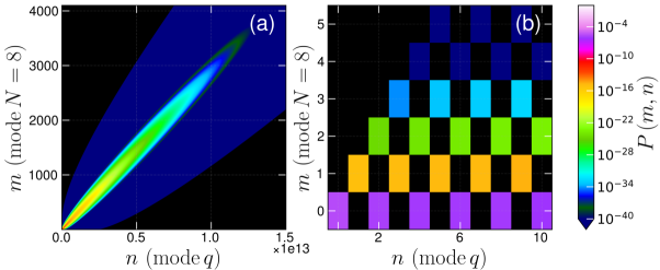
Figure 2: (a) Two-mode probability of QSHHG versus photon number $n$ of the perturbative quantum mode and harmonic photon number $m$ for $N=8$; all parameters and $\langle\hat{n}\rangle_{N}(\theta=0)$ are from Fig. 1(c). (b) Close-up for photon numbers close to zero.

The two-mode distribution (24) is plotted in Fig. 2(a) for harmonic order $N=8$, see Fig. 1(c) for $\langle\hat{n}\rangle_{N}(\theta=0)$; (b) shows a close-up for photon numbers close to zero. The distribution has been calculated numerically from Eqs. (24) and (22). Clearly, harmonic and quantum modes are entangled, as only even-even or odd-odd states are populated. Due to the large value of $r$, the probability extends to very high photon numbers in the quantum mode. The states $m>n$ are approximately zero, accurate to first order in $|\zeta_{N}|^{2}$.

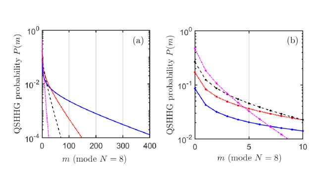
Figure 3: (a) Probability of QSHHG versus harmonic photon number $m$ for $N=8$ (full blue line), $N=10$ (red dotted line), $N=12$ (black dashed line), $N=14$ (magenta dash-dotted line); $m$ refers to number of photons in the QSHH mode $N$; all parameters and $\langle\hat{n}\rangle_{N}(\theta=0)$ are from Fig. 1(c). (b) close-up for photon numbers close to zero.

In Fig. 3(a) the QSHHG probability $P(m)$ is plotted with a closeup in (b). The probability (25) agrees with the probability of a squeezed vacuum state, with the distinction that every photon state is populated and not only the even states. This is a consequence of the two-mode even-even, odd-odd probability distribution. When traced over one of the modes, all number states of the remaining mode are populated and the non-classical features are washed out. Following the above approach, $g^{(2)}(0)$ and the quadrature are obtained, which indicate a super-Poissonian distribution and photon bunching. However no non-classical features, such as squeezing, sub-Poissonian statistics, or a negative Wigner distribution [23, 22] are indicated. In other words, for low conversion efficiency, all combinations of number states are populated and the non-classical features are traced out. However, in the case of unity conversion efficiency, where every BSV photon creates a QSHH photon, and for a single QSHH mode, only even QSHH number states are populated, thereby preserving the non-classical features [35].

For more than one QSHH mode, the entanglement between modes gets more complicated. For example, with three modes, Taylor expansion of Eq. (22) yields operator terms $\sum_{mnj}(\hat{a}_{N}^{\dagger})^{2n+\eta_{n}}(\hat{a}_{N^{\prime}}^{\dagger})^{2m+\eta_{m}}(\hat{a}_{q}^{\dagger})^{j}$, where $\eta_{n},\eta_{m}=0,1$ for even, odd harmonic photon number states, respectively. The expansion coefficient of the squeezed vacuum operator is denoted by $j$ and the photon number of the quantum mode is given by $l=2j+2n+2m+\eta_{n}+\eta_{m}$. As a result, $l$ can only be odd when only one of the harmonic modes is odd: $\eta_{n}=0,1$ and $\eta_{m}=1,0$. When both harmonic modes are odd or even, then $l$ is even. While $l$ can be any positive integer, $n$ and $m$ consist of only even or odd integers for a given $l$, thus resulting in a higher-dimensional checker board pattern similar to Fig. 2. Exploring multi-mode correlation presents an interesting avenue for future work. When the quantum mode is traced over in this three-mode case, all (even-even, odd-odd, and even-odd) states of the two harmonic modes will be populated. It is expected that this will also suppress non-classical properties and entanglement between harmonic modes, for low conversion efficiency.

The focus of the rest of the paper is on single-mode properties of QSHHG. In the following, we demonstrate how non-classical light can be obtained from QSHHG by projective measurements. This relies on the entanglement between quantum and harmonic modes. Projective measurements of entangled wavefunctions generally result in non-classical behavior [38].

III.3 Projective measurement on perturbative quantum mode q

Multi-mode entanglement requires measuring all sidebands simultaneously, or limiting emission to select sidebands only; otherwise, when entangled sidebands are not measured and traced out, mixed states are generated and quantum properties destroyed [38]. Here we discuss the case of one and two sidebands. Our analysis starts with a single sideband, so that the wavefunction is limited to two modes. The number state of the perturbative quantum mode is determined as $|l\rangle_{q}$ by a projective measurement. Determination of the resulting wavefunction starts with a Taylor expansion of the effective two-mode wavefunction (22) followed by a projection on $|l\rangle_{q}$. The projected wavefunction, $\left|\varphi_{N}\right\rangle=\mathbin{{}_{q}\langle}l|\varphi_{m}\rangle$, is found to be [23],

$$\left|\varphi_{N}\right\rangle\!=\!N_{\eta}(-e^{i\theta})^{l/2}\!\sum_{m=0}^{l_{\eta}/2}(-1)^{m}\frac{\sqrt{\alpha_{N}}^{2m+\eta}}{\sqrt{(2m+\eta)!}}\left|2m+\eta\right\rangle_{N}$$

$$\alpha_{N}=\frac{l_{\eta}|\zeta_{N}|^{2}}{2\beta_{N}},\,\,\,l_{\eta}=l-\eta,\,\,\,\,\eta=0,1\,\mathrm{for\,even,odd}\,l$$

$$N_{\eta=0}\approx\frac{1}{\sqrt{\cosh(|\alpha_{N}|)}}\,\,\,\,\,\,N_{\eta=1}\approx\frac{1}{\sqrt{\sinh(|\alpha_{N}|)}}\mathrm{.}$$ (26)

As seen in Fig. 2, the product $\hat{S}_{m}\hat{S}_{q}$ produces either even-even or odd-odd number states. As such, when the projected quantum number $l$ is even ($\eta=0$) or odd ($\eta=1$), the resulting harmonic wavefunction contains only even or odd states, respectively.

From Eq. (26), second order coherence and quadrature of the QSHH modes are calculated. They are a function of the projected quantum mode photon number $l_{\eta}$. Definitions and details on the calculation are given in the supplement; we find [23]

$$g^{(2)}_{N}=\frac{1}{\tanh^{2}(|\alpha_{\mkern-2.0muN}|)}\,\,\,\,\,\,\,\,\mathrm{for}\,\eta=0$$

$$g^{(2)}_{N}=\tanh^{2}(|\alpha_{\mkern-2.0muN}|)\,\,\,\,\,\,\,\,\,\mathrm{for}\,\eta=1\mathrm{}$$ (27)

with the second order coherence $g^{(2)}=(\langle\hat{n}^{2}\rangle-\langle\hat{n}\rangle)/\langle\hat{n}\rangle^{2}$, and

$$\Delta X_{\,jN}^{2}\!=\!\frac{1}{4}\left(1\!+\!2\left(|\alpha_{\mkern-2.0muN}|\tanh(|\alpha_{\mkern-2.0muN}|)\!+\!(-1)^{j}\mathrm{Re}[\alpha_{\mkern-2.0muN}]\right)\!\right)\!\mathrm{,}\,\,\eta=0$$

$$\Delta X_{\,jN}^{2}\!=\!\frac{1}{4}\!\left(\!1\!+\!2\left(\frac{|\alpha_{\mkern-2.0muN}|}{\tanh(|\alpha_{\mkern-2.0muN}|)}\!+\!(-1)^{j}\mathrm{Re}[\alpha_{\mkern-2.0muN}]\right)\!\right)\!\mathrm{,}\,\,\,\,\,\,\,\,\eta=1\mathrm{,}$$ (28)

where $j=1,2$, the quadratures are $\hat{X}_{j}=1/(2i^{j-1})(\hat{a}-(-1)^{j}\hat{a}^{\dagger})$, and the variances $\Delta X_{j}^{2}=\langle\hat{X}_{j}^{2}\rangle-\langle\hat{X}_{j}\rangle^{2}$. All of the above equations were derived for $r\gg 1$, and $l_{\eta}\gg 1$, and give excellent agreement with exact, numerical results in this limit [23]. Even for small $l_{\eta}$, the agreement is surprisingly decent.

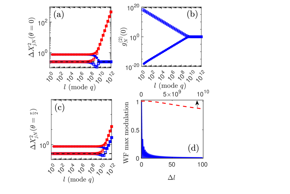
Figure 4: Parameters are the same as in Fig.1; (a-d) $|\zeta_{N}|^{2}(\theta=0)$ taken from $\langle\hat{n}\rangle_{N}$ for $N=8$ in 1(c), respectively. (a),(c) $\Delta X_{jN}^{2}(\theta=0,\pi/2)$ versus quantum photon number $l$, respectively; blue dotted, red full lines show $\Delta X_{jN}^{2}$ for $j=1,2$ respectively; symbols: in (a-c) squares and dots represent $\eta=0,1$ (even, odd states), respectively; symbol spacing follows a $\log$ distribution; black dashed lines indicate quadrature variance of vacuum. (b) second order correlation function $g^{(2)}(0,\theta=0)$ versus $l$. (d) Maximum modulation of Wigner function versus $l+\Delta l$, with $l=10^{10}$ and $\Delta l$ the number state resolution; curves are normalized to the modulation at $\Delta l=0$; blue solid line is for $\Delta l$ even and odd numbers, whereas red dashed line is for $\Delta l$ only even numbers.

The quadrature variances and the second order correlation function are plotted for $N=8$ as a function of quantum mode photon number $l$ in Figs. 4(a),(c) and (b), respectively. The parameter $|\alpha_{N}(\theta)|$ varies with $\theta$ for a given $l$. As such, quadrature variance and second order coherence are $\theta$-dependent. Panels (a,b) are for $\theta=0$ and (c) is for $\theta=\pi/2$. The second order correlation function for $\theta=\pi/2$ is not shown, as it is only quantitatively slightly different.

Note that the sum in the wavefunction (26) has a finite limit $l_{\eta}$. As a result, it goes over into a Schrödinger cat state [38] in the limit $l_{\eta}\rightarrow\infty$, i.e. coherent states with only odd or even number states populated. In the opposite limit $l_{\eta}\rightarrow 0$ it behaves like a heralded number state which through projection is collapsed into a single photon state of the QSHH mode.

The states with only even ($\eta=0$ squares) or only odd ($\eta=1$ dots) photon numbers $l$ behave fundamentally different. In addition, in Figs. 4(a) and (c), blue and red represents the variances $j=1,2$. In the limit of even $l_{\eta=0}\rightarrow 0$, the QSHH distribution has the characteristics of a vacuum number state which has a quadrature variance of $1/4$, see blue and red open squares in Fig. 4(a), and $g^{(2)}(0)\rightarrow\infty$, see open squares in 4(b). The odd states are dominated by a one photon number state which has a quadrature variance of $3/4$, see blue and red dots in Fig. 4(a) and $g^{(2)}(0)\rightarrow 0$, see dots in Fig. 4(b). As such, the odd states, primarily composed of a one photon number state, follow a sub-Poissonian statistics and are highly non-classical. In the intermediate regime, $l\sim 10^{9}-10^{10}$ for (a), moderate squeezing does occur for the even numbered states. In the high $l_{\eta}$ limit, even and odd states merge. All states have the $g^{(2)}(0)=1$ of a coherent state which is typical for Schrödinger cat states. For $\theta=0$, the quadrature $\Delta X_{1}^{2}\rightarrow 1/4$, whereas $\Delta X_{2}^{2}$ grows as a power function. For $\theta=\pi/2$, both quadrature variances grow as power functions.

For the three-mode case, projecting on quantum mode $q$, will separate even-even and odd-odd number state populations for even $l$ from even-odd two-mode states for odd $l$. This results in an entangled two-harmonic mode state which will be subject to future research. However, measuring only one of the two sidebands traces out the other and this likely results in a mixed state, i.e. no quantum features, since the sidebands are entangled [38]. Therefore, all emitted sidebands ought to be measured.

The fact that the projected odd number state ranges from a single photon state to a Schrödinger cat state in dependence on $l_{\eta}$ opens the possibility of quantum engineering QSHHG. Experimental realization is complicated by two facts. (i) The probability of the single photon state is low. (ii) The wavefunction contains even and odd number states; due to the wide range of $l_{\eta}$, it is difficult to resolve number states into single photons. As a result, even and odd states will mix and average out squeezing and the $g^{(2)}_{N}(0)$; for example, amplitude squeezing of the single photon state for low $l$ will be lost.

(i) We find from Fig. 2(b) that the probability of the small $n=l_{\eta}$ odd photon states is dominated by $m=1$ with a probability of $\approx 10^{-15}$. The probability scales as $\propto(|\zeta_{N}|^{2})^{2m+\eta}/\cosh(r)$, and therefore drops fast with increasing $2m+\eta$. As the two-mode probability in Fig. 2(b) is approximately triangular, the one photon number state is essentially pure. Few photon number states $m$ offer less of an advantage; they consist of a superposition of even or odd number states from $n=0$ or $n=1$ up to $n=m$, respectively. Their purity is comparable to that of a finite Schrödinger cat state.

We recall from our discussion of increasing the conversion efficiency of QSHHG below Eq. (23) that it can be increased by more than six orders of magnitude by optimizing material and laser parameters. We decrease $r$ so that the average number of photons, $\hat{n}_{N}=|\zeta_{N}|^{2}\cosh^{2}(r)$ remains constant. As a result $\cosh(r)$ decreases by three orders of magnitude, and the probability of creation of a one photon state increases by nine orders of magnitude to $10^{-6}$. If in addition other parameters are optimized, by for example using a wider pump beam radius, adding another 2 orders of magnitude, a probability for generating a single photon state of about $10^{-4}$ appears achievable. For a MHz laser system, this would mean the generation of a single photon state every $10$ms.

(ii) Techniques for resolving the number of photons are limited to $l\sim 10$ [39]. This gives experimental access to single-photon and few odd-photon states and presents a path to shift the generation of pure heralded single-photon states towards the XUV. In the opposite limit of Schrödinger cat states, $l\gg 1$, projecting on the number state with large $l$ presents a considerable problem for existing technologies. Schrödinger cat states exhibit characteristic interferences near the zeros of the quadratures, with opposite phase shifts for odd- and even-parity states and with varying fringe spacing for different average number of photons. With increasing uncertainty in the photon number resolution, these fringes will be washed out, see Fig. 4(d), where $l=10^{10}$, $\Delta l$ represents the photon number resolution, and the Wigner function is averaged over $\Delta l$. Snapshots of the Wigner function for various $\Delta l$ are shown in the supplement [23]. We show two cases, one with $\Delta l$ running over even and odd numbers (blue full line), and one assuming that parity measurement is possible with $\Delta l$ only extending over even numbers. Without parity measurement, the fringes average out over $100$ number states, for even $\Delta l$ and they vanish immediately for odd $\Delta l$, as even ($l$) and the next odd state ($l+1$) are phase shifted by $\pi$. On the other hand, with the parity measurement, averaging over $10^{10}$ (even only) number states is possible with small losses in the fringe visibility. However, preserving the parity of the quantum mode for such large $l$ is practically impossible, as loosing one photon in $\sim 10^{10}$ would suffice to toggle the parity of the state. The conversion efficiency would have to be increased to levels higher than the typical optical losses of an experiment ($\sim 1\%$) for the parity to be maintained and for the cat state to be measurable. Even without knowledge of parity, a measurement of $g^{(2)}(0)\rightarrow 1$ and of the quadratures’ excess noise by projecting over a range of photon numbers would provide an indication of the generation of the cat states. The quadratures’s noise can be measured in the (few photons) quantum sidebands with homodyne interferometry [40] or, potentially, by extending in-situ techniques to the single shot [29].

III.4 Projective measurement on QSHH mode $N$

The analysis is performed for Eq. (22) with one QSHH mode, i.e. under the assumption that only one sideband is generated. Tracing out the other sidebands in a multi-mode scenario will modify the parameters $\zeta_{N}$ and $\beta_{N}$, but will leave the two-mode wavefunction unchanged otherwise. In a projective measurement, the number of photons $m$ in the effective QSHH mode $N$ is measured. The resulting wavefunction for the quantum mode $q$ depends on $m$ and is calculated by projecting an effective number state on the wavefunction (22) limited to two modes, $|\varphi_{q}\rangle=\mathbin{{}_{N}\langle}m|\varphi_{m}\rangle$. This yields

$$|\varphi_{q}\rangle=N_{m}\sum_{l=0}^{\infty}(-1)^{l}\frac{\sqrt{(2l+m)!}}{l!}\beta_{N}^{l}\left|2l+m\right\rangle_{q}\mathrm{.}$$ (29)

The norm is given by

$$\frac{1}{N_{m}^{2}} \!\approx\frac{\cosh(r)}{\sqrt{1+2\langle\hat{n}\rangle_{\!N}}}\Biggl{[}\!(2m-1)!!\!\left(\frac{\sinh(r)}{1\!+\!2\langle\hat{n}\rangle_{\!N}}\!\right)^{m}$$

$$+\frac{l}{2}(3m-1)(2m-3)!!\left(\frac{\sinh(r)}{1+2\langle\hat{n}\rangle_{\!N}}\right)^{m-1}\Biggr{]}\mathrm{.}$$ (30)

With the above wavefunction second order coherence and quadrature variances are calculated; for definitions and details see the supplement [23]. We obtain for the second order coherence

$$g^{(2)}_{N}(0)\approx 1+\frac{2}{2m+1}\mathrm{.}$$ (31)

The quadratures ($j=1,2$) are found to be

$$\Delta X_{\!jN}^{2} \approx\frac{m(m-1)}{2(2m-1)}\!\!\left(1+(-1)^{j}\cos(\theta)\frac{1+|\zeta_{N}|^{2}}{\tanh r}\right)$$

$$+\frac{(2m\!+\!1)}{4}\frac{A_{j}(r,\theta)+|\zeta_{N}|^{2}(1\!+\!\langle\hat{n}\rangle_{\!N}\!)}{1+2\langle\hat{n}\rangle_{\!N}}\mathrm{}$$ (32)

with $A_{j}(r,\theta)=\cosh^{2}\!r\!+\!\sinh^{2}\!r\!+\!2(-1)^{j}\!\cosh r\sinh r\cos(\theta)$ and $\langle\hat{n}\rangle_{N}=\cosh^{2}\!r|\zeta_{N}|^{2}$. For the case $\theta=0$, $\tanh r\approx 1$, $\langle\hat{n}\rangle_{N}\gg 1$ one obtains

$$\Delta X_{\!jN}^{2}\! \approx\!\frac{2m+1}{4}\frac{(\cosh(r)\!+\!(-1)^{j}\!\sinh(r))^{2}}{1\!+\!2\langle\hat{n}\rangle_{\!N}}$$

$$+\frac{|\zeta_{N}|^{2}}{4}\!\!\left(\!1\!+\!\frac{1}{2(2m\!-\!1)}\!\right)\!\mathrm{.}$$ (33)

We see that the quadrature consists of two contributions; the first term contains the quadrature of a squeezed vacuum state, but has a prefactor that depends on $m$ and $\langle\hat{n}\rangle_{\!N}$. The second term is commonly not part of BSV states. Both modifications come from the mode mixing term $\hat{a}_{N}^{\dagger}\hat{a}_{q}^{\dagger}$ in Eq. (22). Finally, all of the above equations give excellent agreement with the exact, numerical results [23].

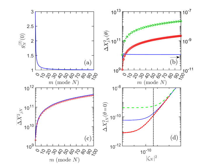
Figure 5: (a) second order correlation $g^{(2)}_{N}(0)$ versus $m$; independent of all other parameters. (b) Quadrature variances $\Delta X_{\,jN}^{2}(\theta)$ ($j=1,2$) for squeezed vacuum angle $\theta$ versus harmonic photon number $m$; evaluated for the effective QSHH order $N=8$; parameters from Fig. 1(b); blue line, red circles for $\theta=0$, $j=1,2$, respectively; black dashed line, green circles (on top) for $\theta=\pi/2$, $j=1,2$, respectively. (c) same as (b), but angle ($\theta$) averaged quadrature variances for $N=8$; blue line, red line with open circles for $j=1,2$, respectively. (d) $\Delta X_{\,1}^{2}(\theta=0)$ evaluated from Eq. (33) versus $|\zeta_{N}|^{2}$ for $m=50$ and for $r=12.4$ (green dashed), $r=13.4$ (full blue), $r=14.4$ (red line with dots); dash-dotted line indicates $|\overline{\zeta}_{N}|^{2}$ of (b) for $N=8$.

The wavefunction in Eq. (29) represents an $m$-photon added squeezed vacuum state [41]. For $m=0$, $g^{(2)}_{N}(0)=3$ takes the value of a squeezed vacuum state, see Fig. 5(a). Further, the product of quadrature variances in Fig. 5(b) for $m=0$ and $\theta=0$ gives $1/16$, the minimum uncertainty. However, the maximum degree of squeezing, occurring for $m=0$ is reduced from that of the input state, which is $\Delta X_{1}^{2}=\frac{1}{4}e^{-2r}\simeq 5\times 10^{-13}$. This can be understood from the fact that mixing between harmonic and quantum modes in QSHHG changes $\beta\rightarrow\beta_{N}$, so that in Eq. (33) a residual term $\propto|\zeta_{N}|^{2}$ remains, even for $m=0$. This term is positive and reduces squeezing, although minimum uncertainty is sustained. Finally, due to mode mixing, the quadrature variances for $m\neq 0$ are different from a regular squeezed state, see blue line and red dots in Fig. 5(b) for $\Delta X_{\,jN}^{2}(\theta=0)$ with $j=1,2$, respectively. Both quadratures increase with $m$, making the state larger than a minimum uncertainty state.

For $\theta=\pi/2$ squeezing disappears, like for a squeezed vacuum beam, see the black dashed line and green circles in Fig. 5(b) for $j=1,2$, respectively. The angle averaged quadrature variance also shows no squeezing, in agreement with a regular squeezed vacuum beam; however $\overline{\Delta X_{\,jN}^{2}}$ with $j=1,2$ need not necessarily be the same, as $|\zeta_{N}(\theta)|^{2}$ is not the same for $\theta$ and $\theta+\pi$, see Fig. 1(c). Finally, Eq. (33) is evaluated for a range of $|\zeta_{N}|^{2}$ for three values of $r$ and for $m=50$; the quadrature variance $\Delta X_{\,1N}^{2}(\theta=0)$ is plotted versus $|\zeta_{N}|^{2}$ in Fig. 5(d). The black dash-dotted line indicates the value of $|\zeta_{N}|^{2}$ in 5(b). The squeezed vacuum parameter exerts large influence for small $|\zeta_{N}|^{2}$ for which the first term in Eq. (33) is dominant. This influence disappears for larger $|\zeta_{N}|^{2}$, where the second term in Eq. (33) dominates. The linear growth highlights that high conversion efficiency compromises the potential for squeezing.

Photon-added squeezed vacuum states have demonstrated an ability to measure phase closer to the Heisenberg limit than other quantum states, such as squeezed vacuum states [42]. Thus, measuring such states during QSHHG seems important. As the projection is done on the (weak) QSHH mode, photon number resolution is less of an issue than in the previous section. The photon added squeezed vacuum state remains a macroscopic state whose quadratures can be measured with conventional homodyne detection [40] or an extension of attosecond techniques such as TIPTOE [43] and nonlinear photoconductive field sampling [44] of quantum fields. Examples of Wigner functions for this state are shown in Fig. (S5) of [23]. The only difficulty is resolving the squeezed quadrature, which can be technically challenging due to saturation of balanced detectors at the high photon fluxes in the quantum mode. However, as discussed above the efficiency of QSHHG can be substantially increased, which allows the use of quantum beams with a much smaller amount of photons. Aside from these technical challenges, an indication of photon added squeezed vacuum states could be obtained experimentally, by measuring the increase of the variance of the quadratures and decrease of $g^{(2)}_{N}(0)$ with increasing $m$.

IV Conclusion

High-harmonic generation is a process that can emit coherent XUV radiation, when driven by sufficiently intense lasers. For classical driving lasers, commonly classical XUV radiation is emitted. When the classical pump laser is replaced by a quantum field, such as a bright squeezed vacuum, properties of high-harmonic generation, such as cutoff and photon statistics (bunching), are modified, however non-classical properties have not been demonstrated yet. In addition, scaling quantum HHG into the XUV regime appears to be challenging.

Quantum sideband high harmonic generation serves as an alternative approach that leverages the strength of readily available intense classical fields to generate the short-wavelength high harmonics, and the quantum properties of a weak perturbing beam to engineer the quantum-optical properties of the harmonics. This imposes less stringent restrictions on the brightness of the quantum perturbation and as such, widens the range of suitable quantum sources.

In this work, a comprehensive theoretical framework of quantum sideband high-harmonic generation has been introduced. It serves as a foundation for designing and developing quantum sideband high-harmonic generation as a short-wavelength attosecond source for quantum light generation. Our theoretical analysis has revealed that quantum sideband high harmonic generation creates entanglement between the harmonic sideband modes and between the harmonic sidebands and the quantum perturbation. The entanglement allows to quantum engineer high harmonic generation via projective measurements. As a result, a variety of states commonly used in quantum information theory can be generated, such as heralded number states, Schrödinger cat states, and photon added squeezed vacuum states. These states will find applications in extending quantum sensing, quantum imaging, and quantum information science to the XUV regime.

Challenges to realize theses states experimentally and potential pathways to overcome them have been discussed. The biggest challenges are (i) the many-mode entanglement between all the sidebands and the BSV and (ii) the low conversion efficiency, which requires BSV beams with a large number of photons; however, still significantly less than what needed to drive high harmonic emission with the BVS field alone.

(i) Multi-mode entanglement requires measuring all sidebands simultaneously to avoid generating a mixed state, when projecting on the BSV. Strategies to monochromatize the emission spectrum were discussed, such as through the use of resonances or phase matching. On the other hand, multi-mode entanglement provides an avenue for creating multi-mode correlations, an interesting avenue for future work.

(ii) The great disparity in photon numbers between sidebands and quantum mode limits the ability to generate, preserve and measure the quantum-optical states, whether generated by direct upconversion or by a projective measurement. This is a common issue when dealing with bright quantum-optical states, and an active area of research. Our simulations reveal that the conversion efficiency scales very favorably with the laser parameters (intensity, wavelength), and the effective mass of the electron, and that near-unity conversion efficiency can potentially be achieved with the help of resonant metasurfaces and optimized phase matching conditions. This boost in efficiency would unlock the potential of high-order sideband generation for the creation of the quantum-optical states predicted in this work.

References

- Krausz and Ivanov [2009] F. Krausz and M. Ivanov, Reviews of Modern Physics 81, 163 (2009).
- Lewenstein et al. [1994] M. Lewenstein, P. Balcou, M. Y. Ivanov, A. L’huillier, and P. Corkum, Physical Review A 49, 2117 (1994).
- Corkum [1993] P. Corkum, Physical Review Letters 71, 1994 (1993).
- Goulielmakis and Brabec [2022] E. Goulielmakis and T. Brabec, Nature Photonics 16, 411 (2022).
- Ghimire et al. [2011] S. Ghimire, A. D. DiChiara, E. Sistrunk, P. Agostini, L. F. DiMauro, and D. A. Reis, Nature physics 7, 138 (2011).
- Gonoskov et al. [2016] I. Gonoskov, N. Tsatrafyllis, I. Kominis, and P. Tzallas, Scientific Reports 6, 32821 (2016).
- Gorlach et al. [2020] A. Gorlach, O. Neufeld, N. Rivera, O. Cohen, and I. Kaminer, Nature Communications 11, 4598 (2020).
- Földi et al. [2021] P. Földi, I. Magashegyi, Á. Gombköto, and S. Varró, in Photonics, Vol. 8 (MDPI, 2021) p. 263.
- Gombkötő et al. [2021] Á. Gombkötő, P. Földi, and S. Varró, Physical Review A 104, 033703 (2021).
- Tsatrafyllis et al. [2019] N. Tsatrafyllis, S. Kühn, M. Dumergue, P. Foldi, S. Kahaly, E. Cormier, I. Gonoskov, B. Kiss, K. Varju, S. Varro, et al., Physical Review Letters 122, 193602 (2019).
- Rivera-Dean et al. [2021] J. Rivera-Dean, P. Stammer, E. Pisanty, T. Lamprou, P. Tzallas, M. Lewenstein, and M. F. Ciappina, Journal of Computational Electronics 20, 2111 (2021).
- Lewenstein et al. [2021] M. Lewenstein, M. F. Ciappina, E. Pisanty, J. Rivera-Dean, P. Stammer, T. Lamprou, and P. Tzallas, Nature Physics 17, 1104 (2021).
- Stammer et al. [2023] P. Stammer, J. Rivera-Dean, A. Maxwell, T. Lamprou, A. Ordóñez, M. F. Ciappina, P. Tzallas, and M. Lewenstein, PRX Quantum 4, 010201 (2023).
- Rivera-Dean et al. [2022] J. Rivera-Dean, P. Stammer, A. S. Maxwell, T. Lamprou, P. Tzallas, M. Lewenstein, and M. F. Ciappina, Physical Review A 106, 063705 (2022).
- Sloan et al. [2023] J. Sloan, A. Gorlach, M. E. Tzur, N. Rivera, O. Cohen, I. Kaminer, and M. Soljačić, arXiv preprint arXiv:2309.16466 (2023).
- Yi et al. [2025] S. Yi, N. D. Klimkin, G. G. Brown, O. Smirnova, S. Patchkovskii, I. Babushkin, and M. Ivanov, Physical Review X 15, 011023 (2025).
- Stammer et al. [2024] P. Stammer, J. Rivera-Dean, A. S. Maxwell, T. Lamprou, J. Argüello-Luengo, P. Tzallas, M. F. Ciappina, and M. Lewenstein, Physical Review Letters 132, 143603 (2024).
- Even Tzur et al. [2023] M. Even Tzur, M. Birk, A. Gorlach, M. Krüger, I. Kaminer, and O. Cohen, Nature Photonics 17, 501 (2023).
- Even Tzur and Cohen [2024] M. Even Tzur and O. Cohen, Light: Science & Applications 13, 41 (2024).
- Rasputnyi et al. [2024] A. Rasputnyi, Z. Chen, M. Birk, O. Cohen, I. Kaminer, M. Krüger, D. Seletskiy, M. Chekhova, and F. Tani, Nature Physics 20, 1960 (2024).
- Heimerl et al. [2024] J. Heimerl, A. Mikhaylov, S. Meier, H. Höllerer, I. Kaminer, M. Chekhova, and P. Hommelhoff, Nature Physics 20, 945 (2024).
- Lemieux et al. [2024] S. Lemieux, S. A. Jalil, D. Purschke, N. Boroumand, D. Villeneuve, A. Naumov, T. Brabec, and G. Vampa, arXiv preprint arXiv:2404.05474 (2024).
- [23] .
- Bertrand et al. [2011] J. Bertrand, H. J. Wörner, H.-C. Bandulet, É. Bisson, M. Spanner, J.-C. Kieffer, D. Villeneuve, and P. B. Corkum, Physical review letters 106, 023001 (2011).
- Purschke et al. [2023] D. N. Purschke, Á. Jiménez-Galán, T. Brabec, A. Y. Naumov, A. Staudte, D. M. Villeneuve, and G. Vampa, Physical Review A 108, L051103 (2023).
- Brunel [1990] F. Brunel, Journal of the Optical Society of America B 7, 521 (1990).
- Vampa et al. [2014] G. Vampa, C. McDonald, G. Orlando, D. Klug, P. Corkum, and T. Brabec, Physical Review Letters 113, 073901 (2014).
- Rohde et al. [2007] P. P. Rohde, W. Mauerer, and C. Silberhorn, New Journal of Physics 9, 91 (2007).
- Dudovich et al. [2006] N. Dudovich, O. Smirnova, J. Levesque, Y. Mairesse, M. Y. Ivanov, D. Villeneuve, and P. B. Corkum, Nature physics 2, 781 (2006).
- Vampa et al. [2015] G. Vampa, T. Hammond, N. Thiré, B. Schmidt, F. Légaré, C. McDonald, T. Brabec, and P. Corkum, Nature 522, 462 (2015).
- Reshak et al. [2014] A. Reshak, Z. Alahmed, and S. Auluck, Solid state sciences 38, 138 (2014).
- Sivis et al. [2017] M. Sivis, M. Taucer, G. Vampa, K. Johnston, A. Staudte, A. Y. Naumov, D. Villeneuve, C. Ropers, and P. Corkum, Science 357, 303 (2017).
- Liu et al. [2018] H. Liu, C. Guo, G. Vampa, J. L. Zhang, T. Sarmiento, M. Xiao, P. H. Bucksbaum, J. Vučković, S. Fan, and D. A. Reis, Nature Physics 14, 1006 (2018).
- Vampa et al. [2017] G. Vampa, B. Ghamsari, S. Siadat Mousavi, T. Hammond, A. Olivieri, E. Lisicka-Skrek, A. Y. Naumov, D. Villeneuve, A. Staudte, P. Berini, et al., Nature Physics 13, 659 (2017).
- Vollmer et al. [2014] C. E. Vollmer, C. Baune, A. Samblowski, T. Eberle, V. Händchen, J. Fiurášek, and R. Schnabel, Physical review letters 112, 073602 (2014).
- Raz et al. [2012] O. Raz, O. Pedatzur, B. D. Bruner, and N. Dudovich, Nature Photonics 6, 170 (2012).
- Uzan et al. [2020] A. J. Uzan, G. Orenstein, Á. Jiménez-Galán, C. McDonald, R. E. Silva, B. D. Bruner, N. D. Klimkin, V. Blanchet, T. Arusi-Parpar, M. Krüger, et al., Nature Photonics 14, 183 (2020).
- Gerry and Knight [2023] C. C. Gerry and P. L. Knight, Introductory quantum optics (Cambridge university press, 2023).
- Schmidt et al. [2018] M. Schmidt, M. Von Helversen, M. López, F. Gericke, E. Schlottmann, T. Heindel, S. Kück, S. Reitzenstein, and J. Beyer, Journal of Low Temperature Physics 193, 1243 (2018).
- Lvovsky [2015] A. I. Lvovsky, Photonics: Scientific Foundations, Technology and Applications 1, 121 (2015).
- Kun et al. [2010] S. Kun, J. Xiao-Hui, and J. Huan-Yu, Chinese Physics B 19, 064205 (2010).
- Guo et al. [2018] L.-L. Guo, Y.-F. Yu, and Z.-M. Zhang, Optics Express 26, 29099 (2018).
- Park et al. [2018] S. B. Park, K. Kim, W. Cho, S. I. Hwang, I. Ivanov, C. H. Nam, and K. T. Kim, Optica 5, 402 (2018).
- Sederberg et al. [2020] S. Sederberg, D. Zimin, S. Keiber, F. Siegrist, M. S. Wismer, V. S. Yakovlev, I. Floss, C. Lemell, J. Burgdörfer, M. Schultze, et al., Nature communications 11, 430 (2020).