TabularQGAN: A Quantum Generative Model for Tabular Data

Abstract

In this paper, we introduce a novel quantum generative model for synthesizing tabular data. Synthetic data is valuable in scenarios where real-world data is scarce or private, it can be used to augment or replace existing datasets. Real-world enterprise data is predominantly tabular and heterogeneous, often comprising a mixture of categorical and numerical features, making it highly relevant across various industries such as healthcare, finance, and software. We propose a quantum generative adversarial network architecture with flexible data encoding and a novel quantum circuit ansatz to effectively model tabular data. The proposed approach is tested on the MIMIC III healthcare and Adult Census datasets, with extensive benchmarking against leading classical models, CTGAN, and CopulaGAN. Experimental results demonstrate that our quantum model outperforms classical models by an average of 8.5% with respect to an overall similarity score from SDMetrics, while using only 0.072% of the parameters of the classical models. Additionally, we evaluate the generalization capabilities of the models using two custom-designed metrics that demonstrate the ability of the proposed quantum model to generate useful and novel samples. To our knowledge, this is one of the first demonstrations of a successful quantum generative model for handling tabular data, indicating that this task could be well-suited to quantum computers.

1 Introduction

Recent progress in quantum computing research for both hardware [1, 2] and algorithmic [3, 4] aspects has been promising. It remains to be shown if quantum computers are universally faster, more energy efficient, or otherwise more useful than classical computers in a task universal to an entire set of problems, apart from areas where it as has been successfully proven: factorization [5], unstructured search [6] and quantum simulation [7].

In this work, we investigate quantum machine learning (QML) models, a class of machine learning model which incorporates quantum computing into a large variety of machine learning architectures and tasks including neural networks [8], reinforcement learning [9], transformers [10, 11], image classification [12], and, the subject of this work, unsupervised generative models, [13]. [14] is a recent overview of the field. As of now, there is no demonstration of QML providing a robust and repeatable advantage over classical methods for practically useful problems [15]. However, a body of evidence suggests that the increased expressivity (i.e., fraction of the parameter sample space can be effectively explored by a variation model) of quantum models may have the same or better performance with a large reduction in the number of parameters required for certain tasks, such as generative learning [16]. Generative QML methods such as Quantum Circuit Born Machines (QCBM) [17, 18] and Quantum GANs (QGAN) [19, 20, 21], have demonstrated comparable training performance to classical models, requiring fewer parameters [22]. QML may be particularly well suited to generative tasks, as the fundamental task of a quantum computer is to produce a probability distribution that is sampled from, which is also what is required for a generative task [23].

Generative models are useful in cases whereby amplifying a sample population with generated samples can lead to improved statistics of rare events [24] (to be used in anomaly detection, fraud identification and market simulations), to improve generative design pipelines (for drug discovery and personalized assistants [25]) and alleviate data privacy concerns by sharing synthetic instead of confidential data [26, 27].

The majority of generative QML research has been on homogeneous data, e.g., image and text data, but business-relevant data is often heterogeneous tabular data, i.e., data that has numeric, categorical, as well as binary features. A prominent example is electronic health records (EHR), which are collections of heterogeneous patient data [28, 29]. Other examples include human resources-related data and chemical structures.

Previous work investigated the use of quantum kernel models in a classification setting of EHR data [30], as well as the use of classical GANs to model EHR data (medGAN) with a reduction of continuous features to a discrete latent space via autoencoding [31]. In addition, the generation of heterogeneous time series data has been investigated, employing variational autoencoders to map the data to and from a smaller latent space for training [32].

In this work, we introduce a novel method for generating tabular data with a QGAN using a custom ansatz (quantum circuit) that does not require additional autoencoding or feature reduction. The model is an adaptation of the model presented in [22]. The architecture makes use of a new approach to model one-hot vectors representing the exclusive categorical features, and is, by construction, well suited to represent numerical features. We perform hyperparameter optimization and benchmark against classical models [33, 34] on subsets of two datasets, MIMIC III [35, 36] and Adult Census [37]. We find that the best-found configurations of the quantum tabular model outperformed the classical model(s) for both datasets.

In section˜2.1 we introduce the mathematical framework of quantum generative models and our approach to modelling one-hot vectors, in section˜2.2, we describe how data is encoded into the quantum circuit, in section˜2.3 we outline the specific architecture of our quantum generative model and how it is trained, followed by an analysis of the resources required from a quantum computer, in section˜2.4. In section˜2.6, the benchmarking and evaluation metrics are outlined. in section˜3.1 details of the datasets are given. In section˜3.2 by the hyperparameter optimization procedure. The experimental configuration and numerical results are presented in section˜3.3. Finally, a discussion of the results, the limitations of our approach, and an outlook is presented in section˜4.

2 Methodology

2.1 Quantum Generative Models and Variational Quantum Circuits

Any generative model is expected to possess two key capabilities: first, the ability to accurately learn the ground truth probability distribution of a provided training dataset, and second, the ability to generalize in order to generate novel samples. In this work, we primarily focus on the ability to learn the ground truth probability distribution and propose a quantum–classical generative adversarial network (QGAN), which has a similar structure to that of a conventional GAN, with the generator implemented using a variational quantum circuit (VQC) [38] and the discriminator is realized using a classical neural network (Figure 2).

A VQC is sequence of parametrized unitary matrices (gates) $U_{m}(\theta_{m})~\in~\mathbb{C}^{2^{n}\times 2^{n}}$ which prepare a quantum state

$$\ket{\Psi(\{\theta_{m}\}_{m})}=\prod_{m}U_{m}(\theta_{m})\ket{\Psi_{0}}~,$$ (1)

starting from an $n$-qubit initial quantum state $\ket{\Psi_{0}}$ of the finite-dimensional Hilbert space $\mathbb{C}^{2^{n}}$, where $U_{m}$ is the gate at index $m$, and $\theta_{m}$ its scalar parameter. The computational basis

$$\left\{\left|i_{1}i_{2}\dots i_{n}\right\rangle\right\}_{i_{1},\ldots,i_{n}\in\{0,1\}}:=\left\{\left|i_{1}\right\rangle\otimes\left|i_{2}\right\rangle\otimes\cdots\left|i_{n}\right\rangle\right\}_{i_{1},\ldots,i_{n}\in\{0,1\}}$$ (2)

is an orthonormal basis for this space and $\left\langle i_{1}i_{2}\dots i_{n}\right|$ the conjugate transpose to the vector $\left|i_{1}i_{2}\dots i_{n}\right\rangle$. Quantum mechanics allows the quantum state $\ket{\Psi(\{\theta_{m}\}_{m})}$ to be a superposition of multiple basis states, which collapses with a probability of

$$p(i_{1}i_{2}\dots i_{n})=|\langle i_{1}i_{2}\dots i_{n}\ket{\Psi(\{\theta_{m}\}_{m})}|^{2}$$ (3)

into the state $\left|i_{1}i_{2}\dots i_{n}\right\rangle$ upon measurement. To employ the VQC as a generator $G$, we encode the rows of a given tabular training set into bitstrings $i_{1}i_{2}\dots i_{n}$ and aim to find a set of parameters $\{\theta_{m}\}_{m}$ such that the probability distribution $p(i_{1}i_{2}\dots i_{n})$ over all bitstrings approximates the underlying probability distribution of the training data. In contrast, the role of the classical discriminator $D:\mathbb{C}^{2^{n}}\rightarrow(0,1)$ is to distinguish if a bitstring $x$ is a genuine (0) or synthetic sample (1). In our experimental evaluation, we consider tabular datasets comprising both numerical and categorical features. Numerical features are modelled using the discrete circuit architecture from [22], while categorical variables are encoded through the application of Givens rotations.

As demonstrated in [39], controlled single-excitation gates implemented as Givens rotations form a universal gate set for particle-conserving unitaries in quantum chemistry. Givens rotations are unitary transformations within a designated subspace of a larger Hilbert space, and we adapt these rotations to preserve the one-hot encoding intrinsic to categorical features. In quantum systems with a fixed excitation number, these rotations facilitate transitions only among basis states that maintain the total number of excitations. For example, in a system comprising of $n$ qubits with exactly $k$ excitations, the relevant subspace is spanned by all states in which exactly $k$ qubits are in the excited state $\ket{1}$ and the remaining $n-k$ qubits are in the ground state $\ket{0}$. The dimensionality of this subspace is d =$\binom{n}{k}$.

To illustrate, consider the encoding of a categorical feature with three distinct categories using one-hot encoding. The encoding is represented by a system of $n=3$ qubits and $k=1$ excitations. An arbitrary rotation among the states $\ket{x_{1}}=\ket{001}$ , $\ket{x_{2}}=\ket{010}$ , $\ket{x_{3}}=\ket{100}$, while leaving other states unchanged, must result in a superposition that strictly maintains the one-hot encoding. The advantage of such a rotation is that it enforces natural symmetry for one-hot encoding. Any arbitrary state given a reference state can be written as $\ket{\psi}=\sum_{i=1}^{d}c_{i}\ket{x_{i}}$. The method for preparing such states is described in [39].

Definition 1 (Hilbert Space Reduction via Givens Rotations)

Let $\mathcal{H}=(\mathbb{C}^{2})^{\otimes n}$ denote the Hilbert space of an $n$-qubit system and define the particle-conserving subspace $\mathcal{H}_{k}\subset\mathcal{H}$ to consist of all states with exactly $k$ excitations (i.e., precisely $k$ qubits in the state $\lvert 1\rangle$ and remainder in state $\lvert 0\rangle$); the dimension of this subspace is $d=\binom{n}{k}$.

Then, any unitary operator $U$ acting on $\mathcal{H}$ that conserves the total number of excitations (i.e., $[U,N]=0$ where $N$ is the excitation number operator) can be decomposed into product of two-level unitary operators known as Givens rotations, $G_{ij}(\theta,\varphi)$, such that

$$U=\prod_{m}G_{i_{m}j_{m}}(\theta_{m},\varphi_{m})$$ (4)

where

$$G_{ij}(\theta,\varphi)=\begin{bmatrix}\cos\theta&-e^{i\varphi}\sin\theta\\ e^{-i\varphi}\sin\theta&\cos\theta\end{bmatrix}$$ (5)

is a gate acting on the subspace of qubit $i$ and $j$, and index $m$ runs over all the gates in the circuit. This decomposition reduces the effective dimensionality of the problem from $2^{n}$ to $\binom{n}{k}$, significantly reducing the parameter space of variational quantum simulations. Givens rotations were originally proposed as gates for quantum chemistry, where conserving the electron number is critical for accurately representing molecular electronic states.

Any state in the subspace $\mathcal{H}_{k}$ can be written as a linear combination of an orthonormal basis $\{\lvert x_{i}\rangle\}_{i=1}^{\binom{n}{k}}$ where each $\lvert x_{i}\rangle$ is a distinct Hamming-weight-k-substring. Since $U$ is a particle-conserving unitary, its action is restricted to $\mathcal{H}_{k}$. Eq. 4 and 5 show that any unitary transformation on a finite-dimensional space can be decomposed into a product of two-level unitary operations (Givens rotations). Each $G_{ij}(\theta,\varphi)$ only affects the amplitudes of the basis states $\lvert x_{i}\rangle$ and $\lvert x_{j}\rangle$ without altering any other state, which ensures that the overall transformation remains within $\mathcal{H}_{k}$.

2.2 Encoding

In this section, we will introduce how the tabular data is encoded into quantum states via basis encoding. Each data sample is mapped to a bitstring of length $n$, which is split into the numerical register, containing ordered variables, and the categorical register containing unordered variables. All numerical variables $x$ are partitioned into $2^{N}$ equal-width bins, where $N$ is the number of qubits allocated to $x$ (the qubit budget). The index $i\in\{0,\dots,2^{N}-1\}$ of the respective bin is represented by a computational-basis state‚

$$\bigl{\lvert}b_{N-1}b_{N-2}\dots b_{0}\bigr{\rangle}~,$$ (6)

where $(b_{N-1}\dots b_{0})$ is the $N$-bit binary expansion of index $i$.

Categorical features with multiple classes ($c>2$), are one-hot encoded using a dedicated $c$-qubit subregister and binary features ($c=2$) are encoded either as Boolean with one qubit $\lvert 0\rangle$ vs. $\lvert 1\rangle$, or one-hot with two qubits: $\lvert 10\rangle$ vs. $\lvert 01\rangle$. This dual-encoding strategy yields two distinct circuit topologies, as shown in Figure 1. The full input register is obtained by concatenating the subregisters for each feature. If feature $f$ uses $N_{f}$ qubits, then an entire record is represented as

$$\bigl{\lvert}\underbrace{b^{(1)}_{N_{1}-1}\dots b^{(1)}_{0}}_{\text{feature 1}}\;\big{\|}\;\underbrace{b^{(2)}_{N_{2}-1}\dots b^{(2)}_{0}}_{\text{feature 2}}\;\big{\|}\;\cdots\bigr{\rangle}$$ (7)

in the computational basis. An explicit example of this encoding can be found in Appendix A.1. We also tested a binary encoding for the categorical features; however, it performed significantly worse in the benchmarking, as shown in Appendix A.2.

2.3 Quantum Generator

We propose two variational circuit designs for the quantum generator: a non-Boolean and a Boolean design. In both designs, the circuit consists of a single $n$-qubit numerical register into which all numerical features are binary encoded, followed by multiple categorical registers, ordered based on the qubit count or number of categories they represent. In the non-Boolean design, all categorical features are encoded in one-hot encoding in (Figure 1), whereas in the Boolean design, encoding of binary categories can be optimized by replacing the one-hot encoding with a Boolean encoding and merging the Boolean variable into the numerical register. The Boolean design saves one qubit per two-category feature. For example, a register configuration in the non-Boolean circuit might be denoted as [n5,c3,c2], where n5 represents a numerical register with five qubits, c3 is a three-qubit one-hot register, and c2 is a two-qubit one-hot categorical register. In Boolean circuit design, the same configuration could be simplified to [n6,c3], where the binary category is absorbed into the numerical register.

Circuit Design: The upper part of the circuit represents an $n$-qubit numerical register which consists of a layer of RY rotations on each qubit, followed by pairwise IsingYY gates and controlled RY rotations. The lower part of the circuit consists of multiple categorical registers. Each categorical register is initialized by an X-gate to prepare a reference state such as $\lvert 1000\rangle$, followed by pairwise single-excitation gates. The entanglement between different registers is established by controlled single-excitation gates to learn correlations between different features.

2.4 Qubit and gate complexity

Let a variational block be applied to a configuration $[\;n,\,c_{1},\,c_{2},\dots,c_{R-1}\;]$ with $R$ registers (1 numerical + $R-1$ categorical). The number of gates required for numerical register ($n$ qubits) is given by

$$g_{\mathrm{num}}(n)=\underbrace{n}_{R_{y}}+\underbrace{(n-1)}_{\text{Ising-YY}}+\underbrace{(n-1)}_{\text{c-}R_{y}}=3n-2~.$$ (8)

For each categorical register of size $c_{i}$, the number of gates will be equal to the number of qubits or the size of the register

$$g_{\mathrm{cat}}(c_{i})=\underbrace{1}_{X\text{-prep}}+\underbrace{(c_{i}-1)}_{\begin{subarray}{c}\text{single-}\\ \text{excitation}\end{subarray}}=c_{i}~.$$ (9)

Cross-register entanglers are controlled single-excitation gate between each adjacent pair of registers

$$g_{\mathrm{cross}}=R-1~.$$ (10)

Hence, the total gate count is

$$g_{\mathrm{total}}=g_{\mathrm{num}}(n)+\sum_{i=1}^{R-1}g_{\mathrm{cat}}(c_{i})+g_{\mathrm{cross}}=\bigl{(}3n-2\bigr{)}+\sum_{i=1}^{R-1}c_{i}+(R-1)~.$$ (11)

Example: $[n_{5},\,c_{3},\,c_{2}]$ ($R=3$)

$$g_{\mathrm{num}}(5)=3\cdot 5-2=13~,\quad g_{\mathrm{cat}}(3)=3,\quad g_{\mathrm{cat}}(2)=2~,\quad$$

$$g_{\mathrm{total}}=13+3+2+2=20~.$$

Let $m=\sum_{i=1}^{R-1}c_{i}$ be the total number of categorical qubits, $R$ be the total number of registers, and $N=n+m$ the overall qubit count. Since $R\leq n+m$, we have

$$g_{\mathrm{total}}=3n-2+m+(R-1)\;=\;O(n+m+R)\;=\;O(N)~.$$ (12)

Thus, for fixed or slowly growing $R$, the total gate count scales linearly with the total number of qubits $N$.

(a) Non-Boolean design

(b) Boolean design

Figure 1: Non-Boolean circuit design (a) and Boolean circuit design (b) for a [n5,c3,c2] register. The model layer can be repeated $d$ times to obtain a depth-$d$ circuit. All qubits are measured in the computational basis to obtain a bitstring generated by the model. Here, the Boolean circuit design saves one qubit by treating the two-category feature as a Boolean variable and merging it into the numerical register.

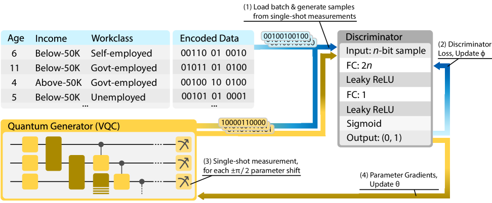
Figure 2: Schematic diagram of TabularQGAN training. In Step 1, either a batch of training data or a batch of synthetic samples (obtained from single-shot measurements) is fed to the discriminator. In Step 2, the discriminator attempts to distinguish between real and fake samples, and its parameters $\phi$ are updated based on the gradient of the discriminator loss $L_{D}$. In Step 3, a sample is generated for each parameter shift, and the discriminator with fixed parameters $\phi$ is used to compute the gradient of the parameters according to the parameter-shift rule. In Step 4, the generator parameters $\theta$ are updated based on their gradient.

2.5 Training QGAN

Training of our TabularQGAN model proceeds by alternately updating a three-layer classical discriminator with a sigmoid output and the quantum generator. The training pipeline is described in Figure 2. First, a batch of $m$ training samples is initialized to $\lvert 0\rangle$ and encoded into the $n$-qubit numerical register and categorical registers. The resulting state $\lvert\psi(\theta,z)\rangle$ is measured in the computational basis to yield bitstrings $x^{\prime}=b_{n-1}b_{n-2}\dots b_{0}$, which are then mapped back to numerical and categorical values. These synthetic samples $x^{\prime}$ are fed into a classical feed-forward network $D(x^{\prime};\phi)$ that outputs $D(x^{\prime})\in(0,1)$, estimating the probability that the input is real. During each training iteration, we first update the parameter vector $\phi$ of the discriminator by minimizing the objective function [40]

$$L_{D}(\phi)=-\frac{1}{m}\sum_{i=1}^{m}\log D(x_{i};\phi)\;-\;\frac{1}{m}\sum_{j=1}^{m}\log\bigl{(}1-D(x^{\prime}_{j};\phi)\bigr{)}~,$$ (13)

where $\{x_{i}\}$ are real records and $\{x^{\prime}_{j}\}$ are generator outputs. Next, we update the generator by fixing $\phi$ and minimizing

$$L_{G}(\theta)=-\frac{1}{m}\sum_{j=1}^{m}\log D(x^{\prime}_{j};\phi)~,$$ (14)

thereby encouraging $G(\theta)$ to produce samples that the discriminator labels as real. Gradients with respect to $\phi$ are computed via standard backpropagation. Gradients with respect to the quantum parameters $\theta$ are obtained using the parameter-shift rule [41][42]: for each parameter $(\theta)$, the gradient is evaluated as derivative of observable $\langle M\rangle$:

$$\frac{\partial\langle M\rangle}{\partial\theta}=\frac{1}{2}\left[\langle M\rangle_{\theta+\frac{\pi}{2}}-\langle M\rangle_{\theta-\frac{\pi}{2}}\right]~,$$ (15)

where $M=D\circ\text{measure on }\left|\psi(\theta,z)\right\rangle$ [43]. The training continues for $T$ epochs or until convergence, monitored via the discriminator loss plateau and sample fidelity metrics (e.g.,  KL divergence). At convergence, the quantum generator has learned to produce synthetic records indistinguishable from real tabular data by the classical discriminator. The training procedure is formally presented in Algorithm 1.

Algorithm 1 TabularQGAN Training Algorithm

Initialize: Generator parameters $\theta$, Discriminator parameters $\phi$, batch size $m$, learning rates $\eta_{G}$, $\eta_{D}$, total epochs/training steps $T$, discriminator steps $k_{D}$

1:for $t=1$ to $T$ do

2:  Discriminator Training:

3:  for $i=1$ to $k_{D}$ do

4:   Sample batch of $m$ examples: $\{x_{1},...,x_{m}\}\sim p_{\mathrm{real}}$

5:   Generate synthetic data:

6:   Prepare quantum state $\lvert\psi\rangle\leftarrow G(\theta)$

7:   Measure and decode: $x^{\prime}\leftarrow\text{Measure}(\lvert\psi\rangle)$

8:   Compute discriminator loss:

$$L_{D}(\phi)=-\frac{1}{m}\sum_{j=1}^{m}\log D(x_{j};\phi)-\frac{1}{m}\sum_{k=1}^{m}\log(1-D(x^{\prime}_{k};\phi))$$

9:   Update discriminator weight: $\phi\leftarrow\phi-\eta_{D}\nabla_{\phi}L_{D}(\phi)$

10:  end for

11:  Generator Training:

12:  Generate synthetic data:

13:  Prepare quantum state for each ($\pm\pi/2$)-parameter shift $\lvert\psi\rangle\leftarrow G(\theta)$

14:  Measure and decode: $x^{\prime}_{j}\leftarrow\text{Measure}(\lvert\psi\rangle)$

15:  Compute generator loss:

$$L_{G}(\theta)=-\frac{1}{m}\sum_{j=1}^{m}\log D(x^{\prime}_{j};\phi)$$

16:  Update generator parameters with parameter-shift rule:

$$\theta\leftarrow\theta-\eta_{G}\nabla_{\theta}L_{G}(\theta)$$

17:  Model Evaluation:

18:  Compute the KL-Divergence between real and generated distributions, to log

19:  it for each epoch for analysis:

$$D_{\text{KL}}(P_{\text{real}}\parallel P_{\text{gen}})=\sum_{x}P_{\text{real}}(x)\log\frac{P_{\text{real}}(x)}{P_{\text{gen}}(x)}$$

20:end for

2.6 Evaluation and Benchmarking

Benchmarks: We benchmark our quantum generator against two classical baselines CTGAN and CopulaGAN. CTGAN is introduced in [33] and CopulaGAN via SDV library [34]. These models are both adaptations of the well-known GAN architecture [44] with additional data preprocessing techniques. These classical benchmarks are chosen as they are also designed specifically for tabular data. All models are trained by minimizing the loss function in Eq. 13.

Evaluation Metrics: We evaluate the performance of the models using three complementary measures: an overall similarity score from SDMetrics [45], the overlap fraction between the training data and synthetic samples, and the final metric measure downstream predictive performance on generated data. The SDMetrics Overall Similarity score [45] is an average over two types of components, column-wise and pairwise metrics. The first is a column-wise measure of univariate marginals, the column shape similarity (See Appendix A.3). The second component is column pair trends, which capture bivariate relations. In addition to these statistical similarity metrics, we also evaluated two measures for measuring the generalisation performance of the models.

The overlap fraction between the training data and the synthetic data is defined as $1~-~(U_{R}~-~U_{S}/U_{R})$ where $U_{R}$ ($U_{S})$ is the count of unique rows in the training (synthetic) data. Hence, an overlap fraction of one would imply that all samples in the synthetic data were also found in the training data.

The second generalization metric, which we call the downstream score, measures how well synthetic data can effectively replace real data in a classical supervised learning task. For each dataset and feature-target combination, we train an XGBoost model [46] on both real and synthetic data using identical hyperparameters and training procedures. If the target is categorical, we report the classification accuracy, and for numerical columns, we report the coefficient of determination $R^{2}$. The downstream score is then defined as the absolute difference between these two performance values: $\text{Downstream Score}\;=\;\bigl{|}\text{Score}_{\mathrm{real}}\;-\;\text{Score}_{\mathrm{synthetic}}\bigr{|}$. A near-zero score indicates that the synthetic data faithfully preserves the predictive relationships found in the original dataset. These metrics collectively quantify the quality and usability of synthetic samples across statistical and downstream learning dimensions.

3 Experimental results

3.1 Dataset

We evaluate our model on two standard datasets, the MIMIC-III clinical dataset [47] and the adult census income dataset [37]. MIMIC-III is a publicly available anonymized health-related data with 100k samples of over forty thousand patients, and the adult census contains income records of adults as per age, education, workclass, etc, with 35k samples. Each dataset contains numerical and categorical features and is divided into 10 and 15-qubit datasets. The number of qubits and features used for each dataset configuration is shown in Table LABEL:tab:dataset_overview.

Table 1: Overview of datasets used in experiments, including the number of qubits, numerical and categorical features.

Dataset Name	Number of Qubits	Numeric Features	Categorical Features
Adults Census 10	10	Age	Income, Education
Adults Census 15	15	Age	Workclass, Education
Mimic 10	10	Age	Gender, Admission type
Mimic 15	15	Age, Admission time	Gender, Admission type

3.2 Hyperparameter Optimization

Hyperparameter optimization was performed over all four data sets for both the quantum and classical models. The optimization was performed via a grid search over the hyperparameters circuit depth, batch size, generator learning rate, discriminator learning rate, and, for the classical models only, layer width. The layer width was either a set value of 256 or data set dependent, as twice the dimension of the training data. Some of the hyperparameter ranges differ between the classical models and the TabularQGAN. This was due to initial experiments indicating which ranges lead to better performance. Each model configuration was repeated five times with a different random seed. The values of the parameters varied are shown in Table 2. For each model, the best hyperparameter settings were selected with respect to the overall metric defined in section 2.6, and can be found in Appendix A.4. In addition to the quantum model, the best epoch of the 3000 epochs was selected (this was not possible for the classical models, as only the parameters for the final epoch were accessible).

Table 2: Hyperparameter settings for each model type, including circuit depth, batch size, learning rates for both the discriminator and generator, layer width, and the number of training epochs.

Model Type	Circuit Depth	% Batch Size	Learning Rate Discriminator	Learning Rate Generator	Layer Width	Number Epochs
TabularQGAN	1, 2, 3, 4	10, 20	0.05, 0.1, 0.2	0.05, 0.1, 0.2	-	3000
CTGAN	1, 2, 3, 4	10, 20	0.001, 0.01, 0.05	0.001, 0.01, 0.05	256	1500
CopulaGAN	1, 2, 3, 4	10, 20	0.001, 0.01, 0.05	0.001, 0.01, 0.05	256	1500

3.3 Results

In this section, we discuss the results of the quantum and classical models with respect to the metrics introduced in Section 2.6. Our experiments are conducted using BASF’s HPC cluster Quriosity, on CPU nodes. All quantum models are executed on noiseless state vector simulations using the PennyLane library. Additional key machine learning libraries used were PyTorch and JAX. Although we described two circuit topologies in Section 2.3, our experiments across four datasets indicate that Boolean and non-Boolean encodings yield comparable performance, see A.5 for more details. Therefore, in this section, we focus exclusively on the results obtained from Boolean-encoding models. The first column in Table 3 shows the results of the overall similarity metric for different models. A score of 1 indicates perfect similarity between the probability distributions of the synthetic and training data sets, whereas 0 implies no similarity. Our TabularQGAN outperforms both classical models, and the performance of CTGAN and CopulaGAN models is similar, see Figure 3. The black-box nature of GAN models makes it challenging to directly attribute the improved performance of the quantum GAN to specific architectural features. However, our hypothesis 2 states that the enhanced expressivity of the quantum circuit and the constrained search space induced by Givens rotations contribute to its improved performance.

Table 3: Best performing models with respect to the overall metric for each data set and model type. The number of parameters is for the best performing hyperparameter configuration.

Data Set	Model Name	Overall Metric	Overlap Fraction	Downstream Score	Number of Parameters
Adults Census 10	TabularQGAN	0.949	0.869	0.026	80
	CTGAN	0.855	0.953	0.112	131,072
	CopulaGAN	0.845	0.953	0.105	65,536
Adults Census 15	TabularQGAN	0.930	0.820	0.038	104
	CTGAN	0.848	0.925	0.117	131,072
	CopulaGAN	0.836	0.913	0.096	60
MIMIC 10	TabularQGAN	0.983	0.973	0.006	88
	CTGAN	0.888	0.984	0.068	65,536
	CopulaGAN	0.887	0.981	0.062	131,072
MIMIC 15	TabularQGAN	0.964	0.784	0.133	37
	CTGAN	0.938	0.770	0.107	262,144
	CopulaGAN	0.924	0.757	0.118	131,072

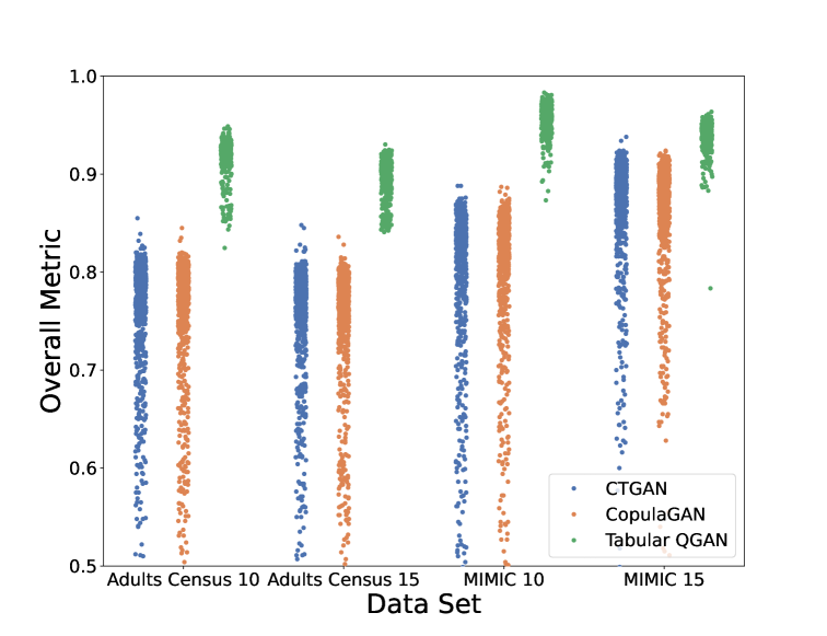
Figure 3: Plot of the overall metric for each hyperparameter configuration for each dataset. The spread of the points within each bar is artificially added to improve data visibility. It can be seen that the TabularQGAN model consistently outperforms the other models.

The second column shows the results of the overlap fraction, which measures the number of unique rows in the synthetic data that are not present in the training data. Due to computational constraints, only a subsample of hyperparameter configurations is evaluated, the best and worst 10 models for each data and model type pair. If the overlap is one, then it implies that no novel samples are generated. The usefulness of the overlap metric for evaluating generalization is limited when applied to low-dimensional datasets such as three features for MIMIC 10 and four features for MIMIC 15. In these cases, the sample space of each data set is mostly covered by the training data set, so novel samples that still fit the underlying distribution are unlikely to be produced. However, our results show that each model does produce some novel samples, meaning they are not purely reproducing the training dataset.

The number of parameters for the optimal configuration of the model varies across the model and data type but for all but one dataset the classical model has far more parameters. The values reported in the last column represent parameter count for the Boolean model configuration. Although the non-Boolean design employs fewer parameters, the difference is minimal. Hence, only the Boolean parameter counts are presented to maintain consistency with the results reported for other models.

In an attempt to find a more qubit-efficient alternative to one-hot encoding, we introduce a Unique-Row-Index encoding and train a generator composed of a single numerical register to reproduce the distribution of row indices (see Appendix A.2). However, the performance of this approach is significantly lower than that achieved with the proposed one-hot encoding with Givens rotations. This suggests that a single numerical register is not a suitable circuit design for generating samples with categorical features.

Analysis of the effect of circuit depth on model performance can be found in Appendix A.6.

4 Conclusion, Limitations and Outlook

In this work, we introduce an adaptation of a quantum GAN model for tabular data. It utilises a novel flexible encoding protocol and circuit ansatz to account for both categorical and numeric data and to natively handle one-hot encoding. In our experiments, the TabularQGAN model outperformed classical models on the datasets under consideration. Additionally, the quantum architecture has significantly fewer parameters than its classical counterparts. Training well-performing models for large-scale real-world applications can require expensive and energy-intensive computation. In this regime, the parameter compression provided by quantum models may dramatically reduce computational resources.

For TabularQGAN to be a practically advantageous model, further investigation is required into the performance as the number of qubits increases. In our current experiments, we limited each dataset to only three to four features for both MIMIC-III and Adult Census datasets which is substantially lower than what is used in many realistic settings. This restriction was made due to the difficulty in simulating models with higher numbers of qubits on classical hardware as currently training on actual quantum hardware is very costly and introduces noise. The difficulty of scaling to larger numbers of qubits has been raised in [48] as the barren plateau problem, and although some quantum architectures have been shown to avoid them [49], it is still an open question if quantum variational models can scale to large qubit counts and avoid classical simulability [50, 51].

Another limitation is that under the data encoding protocol for TabularQGAN, numeric data must be discretized. All the numerical results in this study are based on discretized data; however, in general, classical models do not have such a restriction and may perform better on continuous-valued numeric data.

Further work on testing the model on a wider range of data sets, with a higher number of features, would improve the reliability of the results. Additionally, performing training and sampling at scale on actual quantum hardware would be valuable for understanding the impact of noise on the quality of samples and what might be possible as the size and fidelity of quantum hardware improve. Finally, we considered two variations of a quantum circuit here; more investigation into different ansatz and potential encoding schemes may further improve performance.

5 Acknowledgements

The authors would like to thank the other members of the QUTAC consortium. CJ would also like to thank Abhishek Awasthi and Davide Vodola for their assistance with setting up HPC experiments.

Appendix A Appendices

A.1 Example of Tabular Encoding

In Section 2.2 we introduce a protocol for encoding classical tabular data into quantum states. Here we present an example of that encoding for the Adult Census 10 data set with three features, age, income, and education. The first is a numerical feature age, which is encoded with 5 qubits.
Age (numerical, $N_{\rm age}=5$ qubits $\rightarrow 2^{5}=32$ bins). The width of each bin is calculated from the minimum and maximum values from the training data:

$$W_{\text{age}}=(\{x_{\text{age}}\}_{\text{max}}-\{x_{\text{age}}\}_{\text{min}})~/~\text{Bin Count}$$ (16)

where $W_{\text{age}}$ is the width of each bin and $x_{\text{age}}$ is a vector of the age feature of the training data. The bin number is a rounded value of: $x_{\text{age}}-\{x_{\text{age}}\}_{\text{min}}/W_{\text{age}}$. For example:

$$\text{Age}=19\;\mapsto\;\text{bin }2\;\mapsto\;\lvert 00010\rangle$$

Income is a (binary) variable with options "<=50K" and ">50K". It requires one qubit for Boolean: $\lvert 0\rangle$ (<=50K), $\lvert 1\rangle$ (>50K) and 2-qubits for one-hot: $\lvert 10\rangle$ (<=50K), $\lvert 01\rangle$ (>50K)

Work class is a categorical variable with four options (4 classes, one-hot):

$$(\text{empl-unknown},\lvert 1000\rangle),\;(\text{govt-employed},\lvert 0100\rangle)$$

$$(\text{self-employed},\lvert 0010\rangle),\;(\text{unemployed},\lvert 0001\rangle)$$

A single row is represented as:
Encoding with Boolean design (10 qubits):

$$\{19,\;\text{"<=50K"},\;\text{govt-employed}\}\;\mapsto\;\lvert\,00010\,\|\;0\;\|\;0100\rangle=\lvert 0001000100\rangle$$

Encoding with non-Boolean design (11 qubits):

$$\{19,\;\text{"<=50K"},\;\text{govt-employed}\}\;\mapsto\;\lvert\,00010\,\|\;10\;\|\;0100\rangle=\lvert 00010100100\rangle.$$

A.2 Example of Unique-Row-Index Encoding (Failure Case)

The qubit number required to implement the one-hot encoding introduced in Section 2.2 scales linearly with the number of categories in one feature. It is natural to ask if a more qubit-efficient encoding is possible, while maintaining similarly high benchmarking results.

Consider the following encoding: Assign an index to every unique row of the search space and encode this index as a binary number. We illustrate this encoding with the example from Appendix A.1. The set of all unique rows of the search space is given by

$$\mathcal{S}=\{0,\dots,2^{5}-1\}\times\{\text{Income1},\text{Income2}\}\times\{\text{Workclass1},\dots,\text{Workclass4}\}~,$$ (17)

where $\times$ denotes the Cartesian product of two discrete sets. We assign an index to each of the $|\mathcal{S}|=256$ elements of the set and encode the index in binary using $\log_{2}|\mathcal{S}|=8$ qubits. This allows us to represent all elements of $\mathcal{S}$ using a single numerical register of 8 qubits. We train the circuit to generate indices that follow the underlying distribution of indices in the training data. The generated indices can simply be decoded by directly accessing the corresponding element in $\mathcal{S}$.

We train the model using the proposed Unique-Row-Index encoding on the same hyperparameter ranges described in Section 3.2, applied to both the Adults Census 10 and Adults Census 15 datasets. While scores above 0.9 are achieved on the Adults Census 10 dataset for a few hyperparameter configurations, the performance on the Adults Census 15 dataset is significantly lower (Figure 4). This suggests that a single numerical register is not a suitable circuit design for generating samples with categorical features.

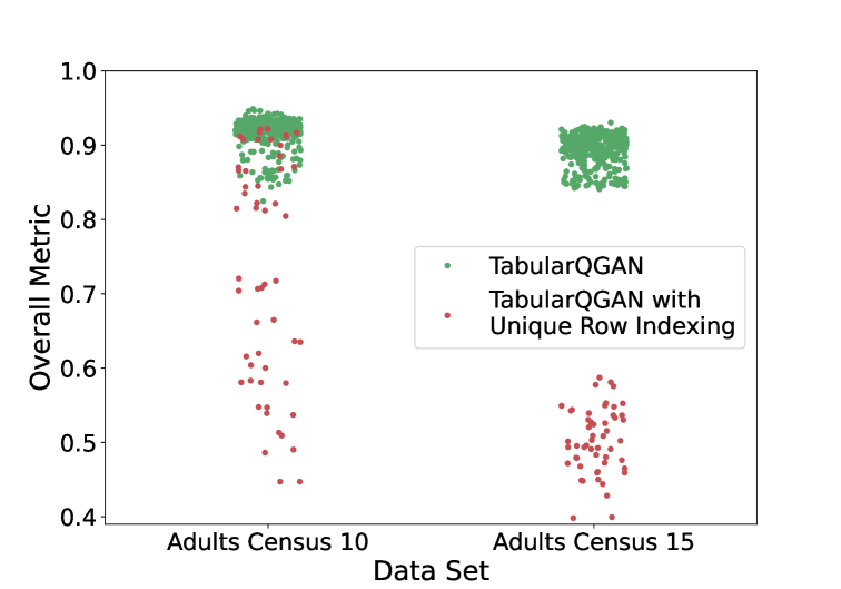
Figure 4: Comparison of the overall metric for each hyperparameter configuration on the Adults Census 10 and Adults Census 15 datasets, using the Unique-Row-Index encoding and a single numerical register for index generation. The spread of points within each bar has been added to improve data visibility. It is evident that the performance of the TabularQGAN model is significantly lower when a Unique-Row-Index encoding is used instead of the proposed one-hot encoding.

A.3 Overall Metric Details

The overall metric, from the SDMetrics library [45], called the overall similarity score there, is an average over two components, the first is a column-wise metric, $S_{\text{shape}}$, and the second is a pairwise metric over each pair of columns $S_{\text{pair}}$.

The column shape metric is given by $S_{\text{shape}}=\frac{1}{C}\sum_{i=1}^{C}s_{i}$ where $C$ is the number of columns and $s_{i}$ is the Kolmogorov–Smirnov complement for numerical columns ($s_{i}=1-\mathrm{KS}(P_{i},Q_{i})$) and the Total Variational Distance Complement for categorical columns ($s_{i}=1-\frac{1}{2}\sum_{k}|P_{i}(k)-Q_{i}(k)|$). Here, $Q_{i}$ is a vector of the values of column $i$ from the training data, and $P_{i}$ is the equivalent for the synthetic data. For the categorical data $Q_{i}(k)$ ($P_{i}(k)$) is the count of the instances of the category $k$ in column $Q_{i}$ ($P_{i}(k)$).

The pair-wise metric is given by $S_{\text{pair}}~=~\frac{1}{\binom{C}{2}}~\sum_{i<j}~t_{ij}$, for columns $i$ and $j$. For numeric data $t_{ij}=1-(|P^{S}_{ij}-P^{R}_{ij}|/2)$ where $P^{S}_{ij}$ and $P^{R}_{ij}$ are the Pearson correlation coefficients for the synthetic and real data, respectively. For categorical data (or a mixed pair of categorical and numeric data), $t_{ij}=1-\frac{1}{2}\sum_{\alpha\in A_{i}}\sum_{\beta\in B_{j}}|F^{S}_{\alpha\beta}-F^{R}_{\alpha\beta}|$. This is the contingency similarity where $\alpha$ is each of the categories of column $A_{i}$, and $F^{S}_{\alpha\beta}$ is the frequency of the category values $\alpha$ and $\beta$ for the synthetic data. Each of these metric are normalized such that they are between $[0,1]$ with 1 being perfect similarity.

Then the final overall metric is an average of the two components. $S_{\text{overall}}=\frac{1}{2}(S_{\text{shape}}+S_{\text{pair}})$.

A.4 Optimum Hyperparameter Configurations

Here we show the hyperparameter configurations associated with our best found models mentioned in Table 3. Each configuration was selected by taking the model instance with the maximum overall metric for each dataset. For TabularQGAN we found that the deeper circuit depths were optimal and for the classical models, the lower number of layers was better.

Table 4: Best found hyperparameter configurations for each model and data type

Data Set Name	Model	% Batch Size	Circuit Depth	LR Gen	LR Discrim	Layer Width	Number Epochs
	TabularQGAN	0.2	4	0.200	0.050	N/A	3000
Adult Census 10	CTGAN	0.2	2	0.001	0.050	256	1500
	CopulaGAN	0.2	1	0.001	0.010	256	1500
	TabularQGAN	0.1	4	0.200	0.100	N/A	3000
Adult Census 15	CTGAN	0.2	2	0.050	0.001	256	1500
	CopulaGAN	0.1	1	0.001	0.050	Data Width	1500
	TabularQGAN	0.2	4	0.100	0.050	N/A	3000
MIMIC 10	CTGAN	0.1	1	0.001	0.010	256	1500
	CopulaGAN	0.1	2	0.001	0.010	256	1500
	TabularQGAN	0.1	1	0.200	0.200	N/A	3000
MIMIC 15	CTGAN	0.1	4	0.001	0.010	256	1500
	CopulaGAN	0.1	2	0.001	0.010	256	1500

A.5 Effect of different Circuit Encodings

We explored two different ways of encoding Boolean variables, with one or two qubits, as described in Section 2.2. We performed the hyperparameter optimization search for each different encoding, for each model type. Figure 5 shows the distributions of the overall metric over the hyperparameter configurations. The distributions for the two different encoding types exhibit high similarity, indicating that the impact of encoding choice was minimal for the features and data sets considered. This limited effect is likely due to the datasets containing at most two Boolean features, which affects only one or two qubits by the current encoding method. However, as the number of Boolean features increases, the influence of encoding choice on performance may become more significant.

A.6 Effect of Circuit Depth on Performance

In Figure 7, the effect of circuit depth for our quantum model and number of layers for the classical models is explored, with the results averaged over all other hyperparameter settings. For the TabularQGAN model (Figure 7(a)), an increasing circuit depth had a small performance improvement for all data sets except for the Adult Census 15 dataset, where there was little difference. The classical models (Figure 7(b)) showed the opposite behavior: increasing the number of layers leads to worse performance. As the classical models had much larger parameter counts, we speculate that this may have been due to excessive overparameterization, which could lead to smaller gradients slowing down, or even stopping, training.

A.7 Overlap Fraction Metric and Downstream Score numerical Results

Figure 6 is a bar plot of the overlap fraction for different model types. It shows that the overlap fraction is well over 50% and close to 1 for some models and data sets. However, we find that the TabularQGAN model has on average a lower overlap score compared to classical models for Adults Census dataset but higher for MIMIC dataset. We find that the overall metric score and the overlap fraction are not correlated for either the classical or quantum models for any data set.

We plot the downstream metric against the overall metric in 8. We split the results into those for classification, Figure 8(a) (where the target feature was categorical), and regression tasks, Figure 8(b) (where the target feature was numeric). Again, these results are for a subsample of the overall hyperparameter-optimized data. We find that, on average, the TabularQGAN models had a lower downstream score, indicating that those samples were better able to replicate the real data in training a classifier. This generalization metric is also contextually useful, for example, in a scenario where the original data, like electronic health records, cannot be shared due to privacy concerns, so that a synthetic dataset can be used instead.

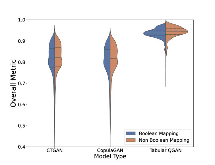
Figure 5: Plot showing the distribution of the overall metric value for each data set with the two different encodings. Adult Census 15 is excluded as it does not contain any binary features.

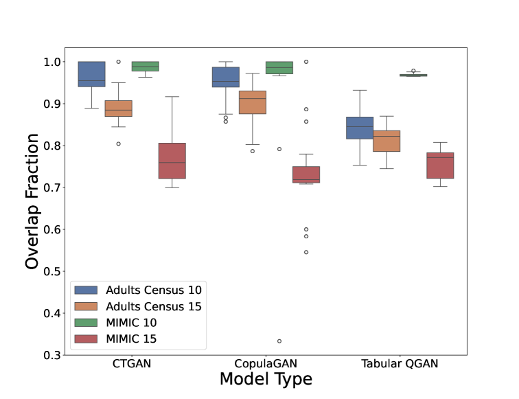
Figure 6: Plot showing the overlap fraction metric for different models and data types. Only a selected subset of the data is sampled.

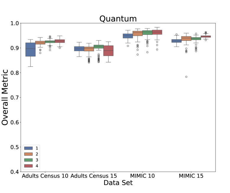
(a)

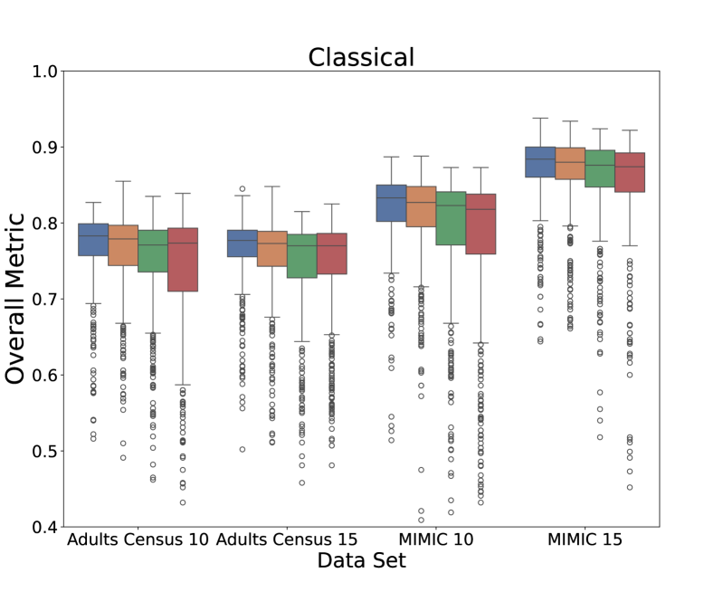
(b)

Figure 7: (a) Effect of circuit depth on performance for quantum models. (b) Effect of the number of layers on performance for classical models. Only data from the Boolean data encoding is included for both plots.

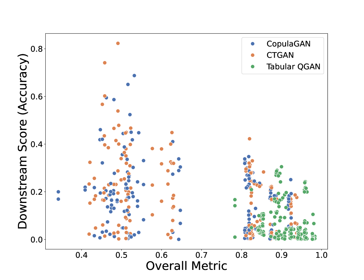
(a)

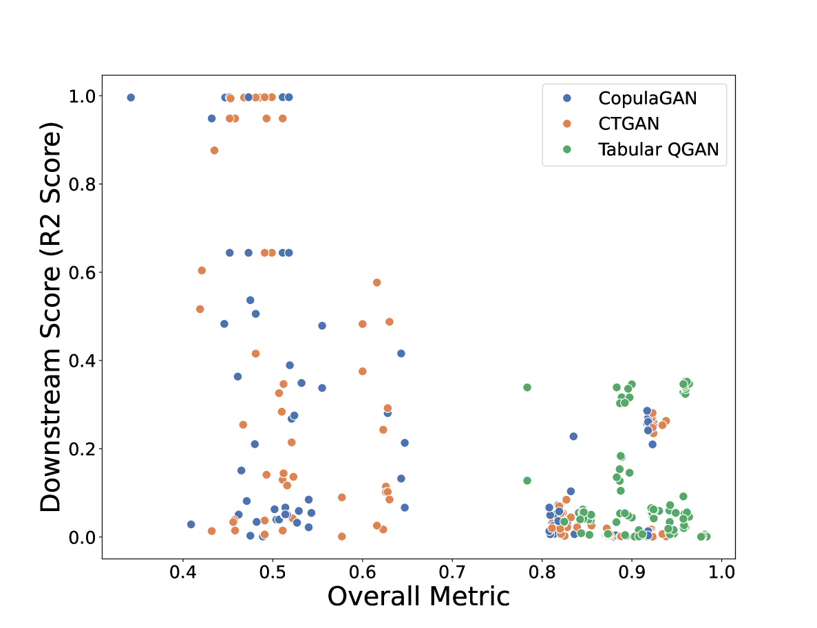
(b)

Figure 8: (a) Downstream Score against Overall Metric for predicting categorical Variables (b) Downstream Score against Overall Metric for predicting numeric Variables. Only a selected subset of the data is sampled.

References

- [1] Rajeev Acharya, Dmitry A Abanin, Laleh Aghababaie-Beni, Igor Aleiner, Trond I Andersen, Markus Ansmann, Frank Arute, Kunal Arya, Abraham Asfaw, Nikita Astrakhantsev, et al. Quantum error correction below the surface code threshold. Nature, 2024.
- [2] Dolev Bluvstein, Simon J. Evered, Alexandra A. Geim, Sophie H. Li, Hengyun Zhou, Tom Manovitz, Sepehr Ebadi, Madelyn Cain, Marcin Kalinowski, Dominik Hangleiter, J. Pablo Bonilla Ataides, Nishad Maskara, Iris Cong, Xun Gao, Pedro Sales Rodriguez, Thomas Karolyshyn, Giulia Semeghini, Michael J. Gullans, Markus Greiner, Vladan Vuletić, and Mikhail D. Lukin. Logical quantum processor based on reconfigurable atom arrays. Nature, pages 1–3, December 2023. Publisher: Nature Publishing Group.
- [3] Youngseok Kim, Andrew Eddins, Sajant Anand, Ken Xuan Wei, Ewout van den Berg, Sami Rosenblatt, Hasan Nayfeh, Yantao Wu, Michael Zaletel, Kristan Temme, and Abhinav Kandala. Evidence for the utility of quantum computing before fault tolerance. Nature, 618(7965):500–505, June 2023. Number: 7965 Publisher: Nature Publishing Group.
- [4] Stephen P Jordan, Noah Shutty, Mary Wootters, Adam Zalcman, Alexander Schmidhuber, Robbie King, Sergei V Isakov, and Ryan Babbush. Optimization by decoded quantum interferometry. arXiv preprint arXiv:2408.08292, 2024.
- [5] Peter W. Shor. Polynomial-time algorithms for prime factorization and discrete logarithms on a quantum computer. SIAM Journal on Computing, 26(5):1484–1509, 1997.
- [6] Lov K. Grover. A fast quantum mechanical algorithm for database search. In Proceedings of the Twenty-Eighth Annual ACM Symposium on Theory of Computing, STOC ’96, page 212–219, New York, NY, USA, 1996. Association for Computing Machinery.
- [7] A Yu Kitaev. Quantum measurements and the abelian stabilizer problem. arXiv preprint quant-ph/9511026, 1995.
- [8] Maria Schuld and Francesco Petruccione. Supervised learning with quantum computers, volume 17. Springer, 2018.
- [9] Artur Garcia-Saez and Jordi Riu. Quantum observables for continuous control of the quantum approximate optimization algorithm via reinforcement learning. arXiv preprint arXiv:1911.09682, 2019.
- [10] El Amine Cherrat, Iordanis Kerenidis, Natansh Mathur, Jonas Landman, Martin Strahm, and Yun Yvonna Li. Quantum vision transformers. arXiv preprint arXiv:2209.08167, 2022.
- [11] Yeqi Gao, Zhao Song, Xin Yang, and Ruizhe Zhang. Fast quantum algorithm for attention computation. arXiv preprint arXiv:2307.08045, 2023.
- [12] Arsenii Senokosov, Alexandr Sedykh, Asel Sagingalieva, Basil Kyriacou, and Alexey Melnikov. Quantum machine learning for image classification. Machine Learning: Science and Technology, 5(1):015040, 2024.
- [13] Ryan Sweke, Jean-Pierre Seifert, Dominik Hangleiter, and Jens Eisert. On the Quantum versus Classical Learnability of Discrete Distributions. Quantum, 5:417, March 2021.
- [14] Yunfei Wang and Junyu Liu. A comprehensive review of quantum machine learning: from nisq to fault tolerance. Reports on Progress in Physics, 2024.
- [15] Joseph Bowles, Shahnawaz Ahmed, and Maria Schuld. Better than classical? the subtle art of benchmarking quantum machine learning models. arXiv preprint arXiv:2403.07059, 2024.
- [16] Amira Abbas, David Sutter, Christa Zoufal, Aurélien Lucchi, Alessio Figalli, and Stefan Woerner. The power of quantum neural networks. Nature Computational Science, 1(6):403–409, 2021.
- [17] Song Cheng, Jing Chen, and Lei Wang. Information perspective to probabilistic modeling: Boltzmann machines versus born machines. Entropy, 20(8), 2018.
- [18] Marcello Benedetti, Delfina Garcia-Pintos, Oscar Perdomo, Vicente Leyton-Ortega, Yunseong Nam, and Alejandro Perdomo-Ortiz. A generative modeling approach for benchmarking and training shallow quantum circuits. npj Quantum Information, 5(1):45, 2019.
- [19] Pierre-Luc Dallaire-Demers and Nathan Killoran. Quantum generative adversarial networks. Phys. Rev. A, 98:012324, Jul 2018.
- [20] Seth Lloyd and Christian Weedbrook. Quantum generative adversarial learning. Physical Review Letters, 121(4), July 2018. arXiv:1804.09139 [quant-ph].
- [21] D. Zhu, N. M. Linke, M. Benedetti, K. A. Landsman, N. H. Nguyen, C. H. Alderete, A. Perdomo-Ortiz, N. Korda, A. Garfoot, C. Brecque, L. Egan, O. Perdomo, and C. Monroe. Training of quantum circuits on a hybrid quantum computer. Science Advances, 5(10):eaaw9918, 2019.
- [22] Carlos A Riofrío, Oliver Mitevski, Caitlin Jones, Florian Krellner, Aleksandar Vučković, Joseph Doetsch, Johannes Klepsch, Thomas Ehmer, and Andre Luckow. A performance characterization of quantum generative models. arXiv e-prints, pages arXiv–2301, 2023.
- [23] X. Gao, Z.-Y. Zhang, and L.-M. Duan. A quantum machine learning algorithm based on generative models. Science Advances, 4(12):eaat9004, 2018.
- [24] Xiangtian Zheng, Bin Wang, Dileep Kalathil, and Le Xie. Generative adversarial networks-based synthetic pmu data creation for improved event classification. IEEE Open Access Journal of Power and Energy, 8:68–76, 2021.
- [25] Xiangxiang Zeng, Fei Wang, Yuan Luo, Seung-gu Kang, Jian Tang, Felice C Lightstone, Evandro F Fang, Wendy Cornell, Ruth Nussinov, and Feixiong Cheng. Deep generative molecular design reshapes drug discovery. Cell Reports Medicine, 3(12), 2022.
- [26] Ismail Keshta and Ammar Odeh. Security and privacy of electronic health records: Concerns and challenges. Egyptian Informatics Journal, 22(2):177–183, 2021.
- [27] Rudolf Mayer, Markus Hittmeir, and Andreas Ekelhart. Privacy-preserving anomaly detection using synthetic data. In IFIP Annual Conference on Data and Applications Security and Privacy, pages 195–207. Springer, 2020.
- [28] Cao Xiao, Edward Choi, and Jimeng Sun. Opportunities and challenges in developing deep learning models using electronic health records data: a systematic review. Journal of the American Medical Informatics Association : JAMIA, 25(10):1419–1428, June 2018.
- [29] Ghadeer Ghosheh, Jin Li, and Tingting Zhu. A review of Generative Adversarial Networks for Electronic Health Records: applications, evaluation measures and data sources, December 2022. arXiv:2203.07018 [cs].
- [30] Zoran Krunic, Frederik F. Flöther, George Seegan, Nathan D. Earnest-Noble, and Omar Shehab. Quantum Kernels for Real-World Predictions Based on Electronic Health Records. IEEE Transactions on Quantum Engineering, 3:1–11, 2022. Conference Name: IEEE Transactions on Quantum Engineering.
- [31] Edward Choi, Siddharth Biswal, Bradley Malin, Jon Duke, Walter F. Stewart, and Jimeng Sun. Generating Multi-label Discrete Patient Records using Generative Adversarial Networks. In Proceedings of the 2nd Machine Learning for Healthcare Conference, pages 286–305. PMLR, November 2017. ISSN: 2640-3498.
- [32] Jin Li, Benjamin J. Cairns, Jingsong Li, and Tingting Zhu. Generating synthetic mixed-type longitudinal electronic health records for artificial intelligent applications. npj Digital Medicine, 6(1):1–18, May 2023. Publisher: Nature Publishing Group.
- [33] Lei Xu, Maria Skoularidou, Alfredo Cuesta-Infante, and Kalyan Veeramachaneni. Modeling tabular data using conditional gan. Advances in neural information processing systems, 32, 2019.
- [34] Neha Patki, Roy Wedge, and Kalyan Veeramachaneni. The synthetic data vault. In IEEE International Conference on Data Science and Advanced Analytics (DSAA), pages 399–410, Oct 2016. Business Source License 1.1.
- [35] Alistair EW Johnson, Tom J Pollard, Lu Shen, Li-wei H Lehman, Mengling Feng, Mohammad Ghassemi, Benjamin Moody, Peter Szolovits, Leo Anthony Celi, and Roger G Mark. Mimic-iii, a freely accessible critical care database. Scientific data, 3(1):1–9, 2016.
- [36] T. & Mark R. Johnson A., Pollard. Mimic-iii clinical database, 2016.
- [37] Barry Becker and Ronny Kohavi. Adult. UCI Machine Learning Repository, 1996. DOI: https://doi.org/10.24432/C5XW20.
- [38] M. Cerezo, Andrew Arrasmith, Ryan Babbush, Simon C. Benjamin, Suguru Endo, Keisuke Fujii, Jarrod R. McClean, Kosuke Mitarai, Xiao Yuan, Lukasz Cincio, and Patrick J. Coles. Variational quantum algorithms. Nature Reviews Physics, 3(9):625–644, 2021.
- [39] Juan Miguel Arrazola, Olivia Di Matteo, Nicolás Quesada, Soran Jahangiri, Alain Delgado, and Nathan Killoran. Universal quantum circuits for quantum chemistry. Quantum, 6:742, June 2022.
- [40] Ian J. Goodfellow, Jean Pouget-Abadie, Mehdi Mirza, Bing Xu, David Warde-Farley, Sherjil Ozair, Aaron Courville, and Yoshua Bengio. Generative adversarial networks, 2014.
- [41] Gavin E. Crooks. Gradients of parameterized quantum gates using the parameter-shift rule and gate decomposition, 2019.
- [42] Maria Schuld, Ville Bergholm, Christian Gogolin, Josh Izaac, and Nathan Killoran. Evaluating analytic gradients on quantum hardware. Physical Review A, 99(3), March 2019.
- [43] René Steijl and George N Barakos. Parallel evaluation of quantum algorithms for computational fluid dynamics. Computers & Fluids, 173:22–28, 2018.
- [44] Ian Goodfellow, Jean Pouget-Abadie, Mehdi Mirza, Bing Xu, David Warde-Farley, Sherjil Ozair, Aaron Courville, and Yoshua Bengio. Generative adversarial nets. In Z. Ghahramani, M. Welling, C. Cortes, N. Lawrence, and K.Q. Weinberger, editors, Advances in Neural Information Processing Systems, volume 27. Curran Associates, Inc., 2014.
- [45] Inc. DataCebo. Synthetic data metrics, 10 2023. Version 0.12.0, MIT License.
- [46] Tianqi Chen and Carlos Guestrin. Xgboost: A scalable tree boosting system. In Proceedings of the 22nd ACM SIGKDD International Conference on Knowledge Discovery and Data Mining, page 785–794. ACM, August 2016.
- [47] Alistair E. W. Johnson, Tom J. Pollard, Lu Shen, Li-wei H. Lehman, Mengling Feng, Mohammad Ghassemi, Benjamin Moody, Peter Szolovits, Leo Anthony Celi, and Roger G. Mark. MIMIC-III, a freely accessible critical care database. Scientific Data, 3(1):160035, May 2016. Number: 1 Publisher: Nature Publishing Group.
- [48] Jarrod R McClean, Sergio Boixo, Vadim N Smelyanskiy, Ryan Babbush, and Hartmut Neven. Barren plateaus in quantum neural network training landscapes. Nature communications, 9(1):4812, 2018.
- [49] Louis Schatzki, Martin Larocca, Quynh T Nguyen, Frederic Sauvage, and Marco Cerezo. Theoretical guarantees for permutation-equivariant quantum neural networks. npj Quantum Information, 10(1):12, 2024.
- [50] Pablo Bermejo, Paolo Braccia, Manuel S Rudolph, Zoë Holmes, Lukasz Cincio, and M Cerezo. Quantum convolutional neural networks are (effectively) classically simulable. arXiv preprint arXiv:2408.12739, 2024.
- [51] Marco Cerezo, Martín Larocca, Diego Garc’ia-Mart’in, N. L. Diaz, Paolo Braccia, Enrico Fontana, Manuel S. Rudolph, Pablo Bermejo, Aroosa Ijaz, Supanut Thanasilp, Eric R Anschuetz, and Zoe Holmes. Does provable absence of barren plateaus imply classical simulability? or, why we need to rethink variational quantum computing. ArXiv, abs/2312.09121, 2023.