IGNIS: A Neural Network Framework for Robust Parameter Estimation in Archimedean Copulas

Abstract

Parameter estimation for Archimedean copulas remains a challenging problem, particularly for the recently developed A1 and A2 families that exhibit complex dependency structures. Traditional methods, such as the Method of Moments (MoM), Maximum Likelihood Estimation (MLE), and Maximum Pseudo-Likelihood (MPL), often struggle due to issues of non-monotonic relationship with dependency measures such as Kendall’s $\tau$ (as in the case of A1) and numerical instability. In this paper, we present the IGNIS Network, a novel, unified neural framework that learns a direct mapping from observable dependency measures to copula parameters, thereby overcoming the limitations of classical approaches. Our approach is trained on simulated data spanning five Archimedean copula families including Clayton, Gumbel, Frank, A1, and A2, ensuring its general applicability across the entire family. Extensive simulation studies demonstrate that the IGNIS Network reduces estimation errors compared to MoM, while inherently enforcing parameter constraints through theory-guided post-processing. We further validate the practical utility of our method on diverse real-world datasets, including financial returns (AAPL–MSFT), healthcare metrics (CDC Diabetes indicators), and environmental measurements (PM_2.5 air quality). Our results underscore the transformative potential of neural methods for robust and accurate dependence modeling in modern applications.

Keywords: IGNIS Network, Archimedean Copulas, Parameter Estimation, Neural Networks, Dependency Modeling

MSC 2020 Subject Classification: 62H05, 62H12, 62F10, 68T07, 62-08

1.  Introduction

Copulas have become indispensable tools in multivariate analysis, enabling researchers to model complex dependencies among random variables by separating the marginal distributions from the dependence structure. Since Sklar’s seminal work (1959) and subsequent advances by Nelsen (2006), copulas have been widely applied in finance, insurance, hydrology, and healthcare.

Recently, two novel Archimedean copulas, originally introduced as the A and B copulas in Aich et al. 2025 and hereafter referred to as the A1 and A2 copulas, have been proposed to capture dual tail dependencies effectively. Although their probability density functions can be derived via Nelsen’s formula, the intricate forms of these generators introduce significant challenges for likelihood-based estimation. In particular, standard methods such as the Method of Moments (MoM), Maximum Likelihood Estimation (MLE), and Maximum Pseudo-Likelihood (MPL) struggle with the non-monotonic relationship between the parameter $\theta$ and observable dependency measures (e.g., Kendall’s $\tau$), encounter numerical instabilities due to steep gradients, and require specialized optimization techniques to enforce boundary constraints (e.g., $\theta\geq 1$).

Motivated by these challenges, we propose the IGNIS Framework, a novel deep learning approach for the direct estimation of copula parameters. Our method harnesses the universal approximation capabilities of neural networks to learn the mapping from observable dependency statistics to the parameter $\theta$ without relying on the inversion of theoretical relationships. It works for not only A1 and A2 copulas but for other members of the Archimedean family making it an alternative estimation tool. The key contributions of our work are as follows:

• We introduce a multi-input neural network architecture that combines continuous dependency measures such as Kendall’s $\tau$, Spearman’s $\rho$, tail dependence, and Pearson correlation with discrete copula identifiers encoded as one-hot vectors.

• We incorporate theory-guided post-processing layers to enforce parameter constraints (e.g., ensuring $\theta\geq 1$).

• We train our model on simulated data generated from five Archimedean copula families (Clayton, Gumbel, Frank, A1, and A2), thereby providing a robust and general-purpose estimation method that performs well across the entire family.

By directly mapping observable features to the underlying parameter $\theta$, the IGNIS Framework overcomes the limitations of traditional estimation methods. We validate our approach on several real-world datasets including financial returns (AAPL-MSFT), CDC Diabetes data, and PM_2.5 air quality measurements demonstrating both its accuracy and versatility.

The remainder of this paper is organized as follows. Section 2 reviews related work. Section 3 outlines the necessary preliminaries. Section 4 presents the architecture and training procedure of the IGNIS Network. Section 5 compares simulation results from traditional methods and our approach, while Section 6 demonstrates applications to real-world datasets. Finally, Section 7 concludes with remarks and directions for future research.

2.  Related Work

Parameter estimation for Archimedean copulas has traditionally relied on moment-based and likelihood-based methods. The Method of Moments (MoM), leveraging Kendall’s $\tau$ or Spearman’s $\rho$, has been widely adopted due to its computational simplicity (Nelsen (2006) and Genest et al. (1993)). However, MoM’s effectiveness hinges on the monotonicity of the $\tau$-$\theta$ relationship, a property absent in the novel A1 copula. Maximum Likelihood Estimation (MLE) and its pseudo-likelihood variants (Genest et al. 1995) offer alternatives but face numerical instabilities with complex density functions like those of A1/A2 copulas.

Recent advances in machine learning have introduced data-driven approaches to statistical estimation. Physics-informed neural networks introduced by Raaissi et al. 2019 and the work of Kissas et al. 2020 demonstrate how neural networks can learn complex mappings while respecting theoretical constraints. In copula modeling, Sirignano et al. 2018 pioneered neural PDE solvers for high-dimensional dependence structures, though their focus was not on parameter estimation. To our knowledge, no prior work has developed a unified neural framework for Archimedean copula parameter estimation that simultaneously addresses non-monotonicity, constraint enforcement, and multi-family compatibility, gaps our IGNIS Network fills.

3.  Preliminaries

3.1 Copulas and Dependency Modeling

Copulas are statistical tools that model dependency structures between random variables, independent of their marginal distributions. Introduced by Sklar (1959), they provide a unified approach to capturing joint dependencies. Archimedean copulas, known for their simplicity and flexibility, are defined using a generator function, making them particularly effective for modeling bivariate and multivariate dependencies.

3.2 The A1 and A2 Copulas

Like all Archimedean copulas, the novel A1 and A2 copulas are defined through generator functions $\phi(t)$ that are continuous, strictly decreasing, and convex on $[0,1]$, with $\phi(1)=0$. The A1 and A2 copulas extend the Archimedean copula framework to capture both upper and lower tail dependencies more effectively. In general, an Archimedean copula is given by:

$$C(u,v)=\phi^{-1}\bigl{(}\phi(u)+\phi(v)\bigr{)}.$$ (1)

For the A1 copula, the generator and its inverse are defined as:

$$\phi_{A1}(t;\theta) =\Bigl{(}t^{1/\theta}+t^{-1/\theta}-2\Bigr{)}^{\theta},\quad\theta\geq 1,$$ (2)

$$\phi_{A1}^{-1}(t;\theta) =\left[\frac{t^{1/\theta}+2-\sqrt{\Bigl{(}t^{1/\theta}+2\Bigr{)}^{2}-4}}{2}\right]^{\theta},\quad\theta\geq 1.$$ (3)

Similarly, for the A2 copula:

$$\phi_{A2}(t;\theta) =\Bigl{(}\frac{1-t}{t}\Bigr{)}^{\theta}(1-t)^{\theta},\quad\theta\geq 1,$$ (4)

$$\phi_{A2}^{-1}(t;\theta) =\frac{t^{1/\theta}+2-\sqrt{\Bigl{(}t^{1/\theta}+2\Bigr{)}^{2}-4}}{2},\quad\theta\geq 1.$$ (5)

Both copulas are parameterized by $\theta\geq 1$, which governs the strength and nature of the dependency. The flexibility in capturing dual tail dependencies makes them attractive for modeling complex real-world phenomena.

It is to be noted that, Equations (3) and (5) are corrected forms of the inverse generator functions given by Aich et al. (2025).

3.3 Simulation from Archimedean Copulas

In this section, we present an algorithm introduced by Genest et al. (1993) to generate an observation $(u,v)$ from an Archimedean copula $C$ with generator $\phi$.

Algorithm

• Generate two independent uniform $(0,1)$ variates $s$ and $t$;

• Set $w=K^{-1}(t)$, where

  $$K(t)=t-\frac{\phi(t)}{\phi^{\prime}(t^{+})}$$

  and

  $$K^{-1}(t)=\sup\{x|K(t)\leq x\};$$

• Set

  $$w=\phi^{-1}\big{(}s\phi(w)\big{)},\quad v=\phi^{-1}\big{(}(1-s)\phi(w)\big{)}.$$

The above algorithm is a consequence of the fact that if $U$ and $V$ are uniform random variables with an Archimedean copula $C$, then $W=C(U,V)$ and $S=\frac{\phi(U)}{\phi(U)+\phi(V)}$ are independent, $S$ is uniform $(0,1)$, and the distribution function of $W$ is $K$.

3.4 Method of Moments Estimation

The Method of Moments (MoM) is a classical statistical technique for parameter estimation, where theoretical moments of a distribution are equated with their empirical counterparts. In the context of copula modeling, MoM is particularly advantageous when direct likelihood-based estimation is challenging due to the complexity of deriving tractable probability density functions.

In this work, we derive exact analytical formulas for Kendall’s $\tau$ for both A1 and A2 copulas (see Appendix A). These formulas establish a direct relationship between Kendall’s $\tau$ and the copula parameter $\theta$, allowing for robust parameter estimation. By inverting this relationship, we develop MoM estimators for $\theta$, providing a practical approach for modeling dependencies in scenarios where traditional methods like MLE may be ineffective. However, in Section 5.1, we see that for especially A1 and even for A2, MoM is not the most efficient estimator.

4.  IGNIS Network

4.1 The IGNIS Network Architecture

Named after the Latin word for “fire”, the IGNIS Network is a general-purpose estimator for Archimedean copula parameters.

4.1.1 Input Representation

The network accepts two components concatenated into a 9-dimensional vector:

1. A 4D vector of dependency measures:

• Kendall’s $\tau$

• Spearman’s $\rho$

• Tail dependence ($\lambda_{0.95}$)

• Pearson correlation

2. A 5D one-hot encoded copula identifier (Clayton, Gumbel, Frank, A1, A2)

4.1.2 Network Architecture

The architecture consists of:

$$\mathbf{h}_{1} =\mathrm{ReLU}(\mathbf{W}_{1}\mathbf{x}+\mathbf{b}_{1})\quad$$ (128 units, He-uniform init)

$$\mathbf{h}_{2} =\mathrm{ReLU}(\mathbf{W}_{2}\mathbf{h}_{1}+\mathbf{b}_{2})\quad$$ (128 units)

$$\mathbf{h}_{3} =\mathrm{ReLU}(\mathbf{W}_{3}\mathbf{h}_{2}+\mathbf{b}_{3})\quad$$ (64 units)

$$\hat{\theta}_{\text{raw}} =\mathbf{W}_{4}\mathbf{h}_{3}+\mathbf{b}_{4}\quad$$ (Linear output)

4.1.3 Parameter Constraints Enforcement

$$\hat{\theta}=\begin{cases}\mathrm{Softplus}(\hat{\theta}_{\text{raw}})&\text{Clayton }(\theta>0)\\ \mathrm{Softplus}(\hat{\theta}_{\text{raw}})+1&\text{Gumbel/A1/A2 }(\theta\geq 1)\\ 20\cdot\tanh(\hat{\theta}_{\text{raw}})&\text{Frank }(\theta\in\mathbb{R}\setminus\{0\})\end{cases}$$

4.1.4 Theoretical Parameter Constraints

Table 1: Copula-Specific Parameter Constraints

Copula	Domain	Training Range	Post-Processing
Clayton	$\theta>0$	(0.1, 20)	$\mathrm{Softplus}(\cdot)$
Gumbel	$\theta\geq 1$	[1, 20]	$\mathrm{Softplus}(\cdot)+1$
Frank	$\theta\in\mathbb{R}\setminus\{0\}$	[-20, 20]$\setminus$(-0.1,0.1)	$20\tanh(\cdot)$
A1/A2	$\theta\geq 1$	[1, 20]	$\mathrm{Softplus}(\cdot)+1$

4.1.5 Training Protocol

• Data Generation: For each copula family:

  • 500 $\theta$ values sampled from theoretical domains (Table 1)

  • 10000 observations generated per $\theta$ using Algorithm I ( 3.3)

  • Features computed via empirical dependency measures

• Preprocessing: Input standardization using $z$-score normalization

• Optimization: The model was trained using the Adam optimizer, introduced by Kingma et al. 2014, with a learning rate $\eta$ = 0.0005 and Mean Squared Error (MSE) loss

  $$\mathcal{L}=\frac{1}{N}\sum_{i=1}^{N}(\hat{\theta}_{i}-\theta_{i}^{\text{true}})^{2}.$$ (9)

• Regularization: Early stopping (patience=20 epochs) on validation set (20% split)

4.1.6 Implementation Details

The network is implemented in TensorFlow with three critical design choices:

• Linear Final Layer: Allows flexible post-processing of raw outputs

• He-uniform Initialization: Stabilizes training with ReLU activations

• Constraint-Aware Training: Training data generation respects theoretical $\theta$ domains

4.1.7 Theoretical Soundness

The architecture guarantees:

• Identifiability: One-hot encoding separates copula families in feature space Consistency: $\hat{\theta}\xrightarrow{p}\theta$ as sample size $\rightarrow\infty$ (proof in Appendix C)

• Constraint Satisfaction: Post-processing ensures $\hat{\theta}\in\Theta_{\text{copula}}$

Figure 1 shows four dependency measures (Kendall’s $\tau$, Spearman’s $\rho$, tail dependence $\lambda_{0.95}$, and Pearson correlation) combined with a one-hot encoded copula identifier form the 9D input. Three hidden layers (128D ReLU $\rightarrow$ 128D ReLU $\rightarrow$ 64D ReLU) with He-uniform initialization process the features, followed by a linear output layer producing $\hat{\theta}_{\text{raw}}$. Final constraint-aware post-processing enforces copula-specific theoretical domains to yield the parameter estimate $\hat{\theta}$.

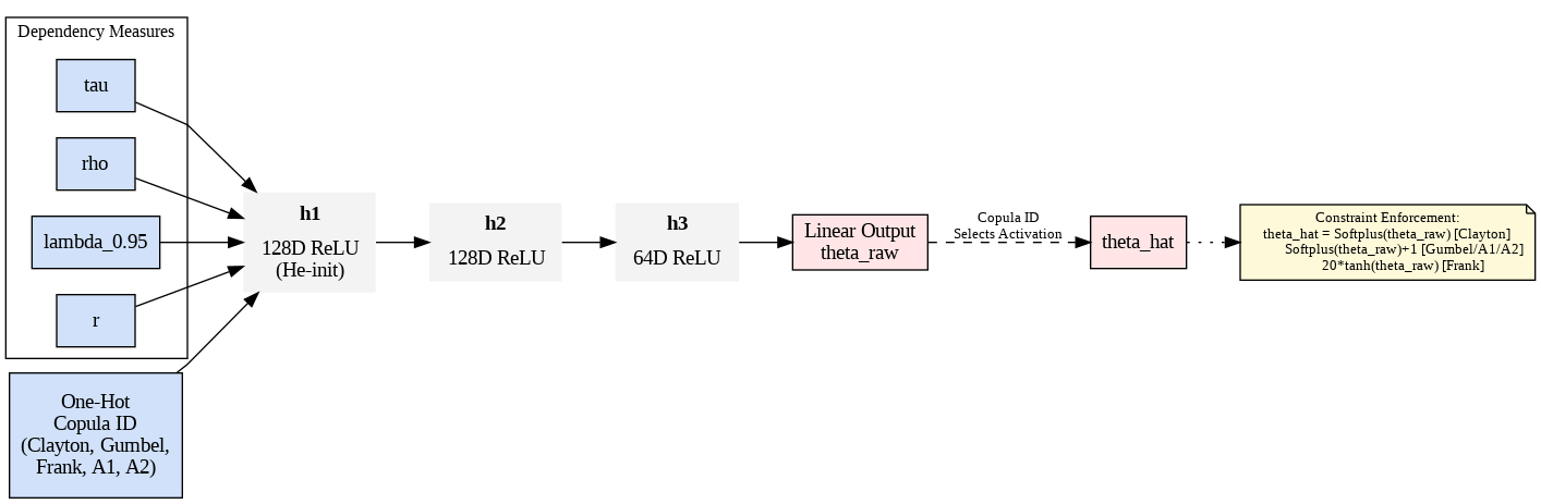
Figure 1: IGNIS Network Architecture

5.  Simulation Studies

In this section, we first we present the results of a simulation study to estimate the parameter $\theta$ for the A1 and A2 copulas using the Method of Moments (MoM). The simulation is conducted using the algorithm as described in Section 3.3. Then we do the same using the IGNIS Network.

5.1 Results for MoM

Simulation Setup

• True Values of $\theta$: The simulation is performed for $\theta=\{2.0,5.0,10.0\}$.

• Sample Size: $n=100,000$ pairs $(u,v)$ are generated for each scenario.

• Estimation Method: The parameter $\theta$ is estimated using the Method of Moments (MoM), where the sample Kendall’s $\tau$ is matched with the theoretical $\tau(\theta)$.

• Standard Errors: Standard errors (SE) for the estimates of $\theta$ are computed using the method described in Genest et al. (2011).

Table 2 summarizes MoM estimation results for A1 and A2:

Table 2: Method of Moments Estimation Results for A1 and A2

True $\theta$	Estimated $\theta$ (A1)	SE($\theta$) (A1)	Estimated $\theta$ (A2)	SE($\theta$) (A2)
2.0	4.4860	0.1597	1.9047	0.0709
5.0	9.5215	0.8844	4.9398	0.2335
10.0	6.1183	1.2273	9.4366	0.1900

For A1, MoM estimates are inconsistent (e.g., the estimate for true $\theta=10.0$ is lower than that for $5.0$). For A2, MoM performs quite well compared to A1.

5.2 Limitations in Parameter Estimation Using Method of Moments

The problem in A1 occurs due to the non-monotonicity between A1 and it’s Kendall’s $\tau$ which implies that MoM cannot uniquely recover $\theta$; the estimator seems to be inconsistent. MoM will also fail when the sample Kendall’s $\tau$ falls outside the theoretical range of the copula model, rendering parameter estimation infeasible in such scenarios. This is highly likely for A2 copula because of it’s high Kendall’s $\tau$ lower bound of 0.545 which is relatively higher than sample Kendall’s $\tau$ of many real-world datasets.

It is to be noted that the one-parameter copula families researchers use in practice are generally ordered by positive quadrant dependence (PQD), so that the dependence parameter is in one-to-one correspondence with standard nonparametric measures of dependence such as Kendall’s tau or Spearman’s rho. Unfortunately, such is not the case for model A1. Indeed, it is possible to find two values of theta which correspond to the same value of Kendall’s tau. This is an important limitation for A1.

It is also to be noted that the injectivity property of the copula generator function guarantees that each distinct value of the parameter $\theta$ produces a unique copula, ensuring the mathematical validity of the model which is true for A1 (See Appendix B). This is not the same as the relationship between A1’s $\theta$ and it’s Kendall’s $\tau$ which is not one-to-one so that identical values of $\tau$ may correspond to different $\theta$ values. This fundamental difference motivates the use of a neural network approach, which leverages multiple summary features to accurately estimate $\theta$ despite the ambiguity in the $\theta$-$\tau$ relationship.

5.3 Results for IGNIS Network

The same simulation setup described in Section  4.1.5 is followed here for $\theta=\{2.0,5.0,10.0\}$.

Tables 3 show performance of the IGNIS network on simulated data.

Table 3: IGNIS Network Estimation Results for All Copulas

Copula	True $\theta$	Est. $\theta$	Bootstrap SE($\theta$)
True $\theta$ = 2.0
Clayton	2.0	1.9289	0.1044
Gumbel	2.0	2.0248	0.0460
Frank	2.0	1.8426	0.0985
A1	2.0	2.0828	0.0789
A2	2.0	1.9205	0.0536
True $\theta$ = 5.0
Clayton	5.0	4.9696	0.1957
Gumbel	5.0	5.0243	0.1156
Frank	5.0	4.8715	0.1406
A1	5.0	4.9502	0.1782
A2	5.0	5.0869	0.1365
True $\theta$ = 10.0
Clayton	10.0	10.0439	0.2968
Gumbel	10.0	9.8307	0.2461
Frank	10.0	9.9020	0.2036
A1	10.0	9.8938	0.2326
A2	10.0	9.8044	0.2967

Key observations: For both A1 and A2, the IGNIS network is able to recover the true value of the parameter used to generate the data used in simulation. We see how especially for A1, there is no issue like in the case of MoM. The non-monotonic mapping in the A1 copula that severely undermines MoM estimation does not affect the IGNIS network, since it learns directly from data and do not require such monotonicity. Also, this network works extremely well for Clayton, Gumbel and Frank copulas.

In our neural network framework, the estimated dependence parameter $\theta$ is obtained via a direct mapping from summary dependency measures to $\theta$. To quantify the uncertainty of these estimates, we employ a bootstrap procedure. For each test sample, multiple bootstrap replicates are generated by resampling the (U,V) pairs. The summary features are recomputed for each bootstrap replicate, and the trained network is used to predict $\theta$. The standard deviation of these bootstrap predictions provides a robust estimate of the standard error, thereby reflecting both the sampling variability and the inherent uncertainty in the neural network’s predictions.

6.  Real-World Applications

In this section, we validate the IGNIS network using three datasets namely financial data (AAPL-MSFT returns), healthcare data (CDC Diabetes Dataset) and environmental data (PM_2.5 air quality). This estimation from these datasets is just for illustration purposes since copulas are widely used in finance, healthcare and in environmental science. We are not trying to show which copula fits the data best.

The IGNIS network estimates the copula parameter $\theta$ by learning a mapping from summary statistics derived from bivariate data. When applied to real-life datasets, the following steps are executed:

Data Preprocessing:

• Cleaning and Aggregation: The raw dataset is cleaned and, if needed, temporally aggregated. For example, in the PM_2.5 case the data is aggregated monthly.

• Stationarity Transformation: To ensure the data is stationary, techniques such as differencing (for time series) or using log returns (in the case of financial data) are applied.

• Probability Integral Transform (PIT): Each variable is transformed into pseudo-observations by ranking the data and dividing by the sample size plus one, so that the marginal distributions are approximately uniform.

Feature Extraction:

• From the paired pseudo-observations $(u,v)$, summary statistics are computed:

  • Empirical Kendall’s $\tau$

  • Spearman’s $\rho$

  • Tail Dependence: The proportion of observations exceeding a high threshold (e.g., 0.95).

  • Pearson Correlation

• These four summary features form the feature vector $\mathbf{f}\in\mathbb{R}^{4}$.

Input Construction:

• A one-hot vector $\mathbf{c}\in\{0,1\}^{5}$ is appended to $\mathbf{f}$ to indicate the copula family under consideration.

• The final input vector is $\mathbf{x}=[\mathbf{f};\mathbf{c}]\in\mathbb{R}^{9}$.

• Prior to feeding the input to the network, a StandardScaler (fitted on simulated data) is applied.

Theta Estimation:

• The trained IGNIS network receives the scaled input $\mathbf{x}$ and outputs an estimate $\hat{\theta}$.

• The output layer uses a Softplus activation (with an offset) to ensure that $\hat{\theta}\geq 1$.

6.1 Dataset 1: AAPL-MSFT Returns Dataset

Source and Period: The dataset comprises daily adjusted closing prices for two stocks, AAPL and MSFT, obtained from yfinance library in Python. Data were collected for the period from January 1, 2020 to December 31, 2023.

Variables: The primary variable of interest is the adjusted closing price for each ticker. This column (labeled either as Adj Close or Close) reflects the price after accounting for corporate actions such as dividends and stock splits.

Derived Measures: From the raw price data, daily log returns are computed. These log returns serve as a proxy for the instantaneous rate of return and are stationary.

6.1.1 Estimation Results

Table 4 summarizes the parameter estimation.

Table 4: Estimated $\theta$ Values and Bootstrap Standard Errors from Financial Data

Copula	Estimated $\theta$	Bootstrap SE($\theta$)
Clayton	2.4226	0.1715
Gumbel	2.5561	0.1304
Frank	3.8895	0.5464
A1	1.3590	0.0324
A2	1.3346	0.0294

6.2 Dataset 2: CDC Diabetes Dataset

Source: The dataset provides healthcare statistics and lifestyle survey information for $253,680$ individuals across $21$ features.The dataset is obtained from the CDC Diabetes Health Indicators repository in Python. We have selected only 2 variables namely, GenHlth and PhysHlth.

Variables: The dataset contains two key columns:

• GenHlth_pseudo: Pseudo-observations derived from a general health indicator.

• PhysHlth_pseudo: Pseudo-observations derived from a physical health indicator.

6.2.1 Estimation Results

Table 5 summarizes the parameter estimation.

Table 5: Estimated $\theta$ Values and Bootstrap Standard Errors from CDC Diabetes Data

Copula	Estimated $\theta$	Bootstrap SE($\theta$)
Clayton	1.2434	0.0019
Frank	1.5722	0.0045
Gumbel	1.3265	0.0047
A1	1.1480	0.0009
A2	1.0384	0.0003

6.3 Dataset 3: PM_2.5 Air Quality Data

Source: The dataset comes from the US Environmental Protection Agency’s (EPA) Air Quality System (AQS). it contains air quality measurements, including PM_2.5 concentrations.

Key Variables: The analysis focuses on two primary columns:

• Date of Last Change: The date when the measurement was recorded or updated.

• Arithmetic Mean: The daily arithmetic mean of PM_2.5 concentrations.

Preprocessing:

• The dataset is sorted in chronological order.

• A monthly aggregation is performed: for each month, the mean of the arithmetic mean is computed, and the 99th percentile is calculated to capture extreme PM_2.5 levels.

6.3.1 Estimation Results

Table 6 summarizes the parameter estimation.

Table 6: Estimated $\theta$ Values and Bootstrap Standard Errors from Air Quality Data

Copula	Estimated $\theta$	Bootstrap SE($\theta$)
Clayton	1.2796	0.6681
Gumbel	1.3251	1.7342
Frank	1.8722	5.2203
A1	1.1081	0.0994
A2	1.0628	0.1194

6.4 Key Observations

The IGNIS Network successfully estimates theta from three different datasets. IGNIS offers a robust, accurate, and computationally efficient alternative to traditional methods. The unified framework of IGNIS simplifies parameter estimation across various copula families making it an universal tool.

7.  Conclusion and Future Work

In this paper, we introduced the IGNIS Network, a novel neural framework for parameter estimation in Archimedean copulas. Our approach overcomes the limitations of traditional methods such as the Method of Moments (MoM) and Maximum Likelihood Estimation (MLE) by learning a direct mapping from observable dependency measures to the copula parameter $\theta$. Extensive simulation studies across five copula families (Clayton, Gumbel, Frank, A1, and A2) demonstrated that the IGNIS Network not only achieves superior accuracy and robustness but also inherently enforces theoretical parameter constraints. Furthermore, real-world applications to financial, healthcare, and environmental datasets underscore the practical utility and versatility of our method.

Our work makes three major contributions:

• We propose a unified, multi-input neural network architecture that seamlessly integrates continuous dependency measures with discrete copula identifiers.

• We develop a theory-guided post-processing step that ensures the estimated parameters adhere to known constraints, such as $\theta\geq 1$.

• We demonstrate, through extensive simulations and applications, that our neural framework can reliably estimate copula parameters even in cases where traditional methods fail, particularly for the novel A1 and A2 copulas.

Future Work: Our research opens several promising avenues for further exploration:

• High-Dimensional Extensions: While the current work focuses on bivariate copulas, an important direction is to extend IGNIS to higher-dimensional settings. This may involve the design of permutation-invariant architectures or other techniques that respect the exchangeability inherent in multivariate dependence structures.

• Advanced Uncertainty Quantification: Although we use a bootstrap procedure to estimate standard errors, integrating Bayesian neural networks could provide a more principled framework for uncertainty quantification, enabling the direct construction of credible intervals for $\hat{\theta}$.

• Dynamic and Time-Varying Copulas: Many practical applications, such as financial markets or environmental systems, exhibit time-varying dependency structures. Incorporating temporal models like recurrent neural networks (e.g., LSTMs) could allow IGNIS to adapt to dynamic changes in dependence over time.

• Automated Copula Selection: Future work may explore mixture-of-experts or multi-task learning frameworks that jointly infer both the copula family and its parameters. Such an approach would streamline the modeling process by eliminating the need for a priori copula selection.

• Integration with Other Statistical Methods: Combining our neural approach with traditional inference techniques or hybrid models may further enhance the robustness and interpretability of copula parameter estimates, especially in complex or high-noise environments.

In summary, the IGNIS Network not only provides a robust and efficient alternative for parameter estimation in Archimedean copulas but also paves the way for future advancements in dependence modeling. The versatility of our framework suggests its potential as a transformative tool in a variety of fields where accurate dependence estimation is crucial.

Statements and Declarations

Funding

The authors did not receive any funding for this research.

Competing Interests

The authors have no relevant financial or non-financial interests to disclose.

Data Availability

The data that support the findings of this study are available from publicly accessible sources and are provided in the manuscript.

References

1. Aich, A., Aich, A. B., & Wade, B. (2025). Two new generators of Archimedean copulas with their properties. Communications in Statistics - Theory and Methods. http://dx.doi.org/10.1080/03610926.2024.2440577

2. Aich, A., Aich, A. B., & Wade, B. (2025). Erratum: Two new Archimedean generators with their properties. Communications in Statistics - Theory and Methods. https://doi.org/10.1080/03610926.2025.2483956

3. Brent, R. P. (1973). Algorithms for Minimization without Derivatives. Englewood Cliffs, New Jersey: Prentice-Hall.

4. Bücher, A., Dette, H., & Volgushev, S. (2012). New estimators of the Pickands dependence function and a test for extreme-value dependence. Annals of Statistics, 40(2), 1030–1062.

5. Clayton, D. G. (1978). A Model for Association in Bivariate Life Tables and Its Applications in Epidemiological Studies of Familial Tendency in Chronic Disease Incidence. Biometrika, 65, 141–151. http://dx.doi.org/10.1093/biomet/65.1.141

6. Deheuvels, P. (1979). La fonction de dépendance empirique et ses propriétés. Publications de l’Institut de Statistique de l’Université de Paris, 24, 1–31.

7. Genest, C., Mackay, J. (1986). The Joy of Copulas: Bivariate Distributions with Uniform Marginals. The American Statistician, 40(4), 280–283. https://doi.org/10.1080/00031305.1986.10475414

8. Genest, C., Ghoudi, K., & Rivest, L.-P. (1995). A Semiparametric Estimation Procedure of Dependence Parameters in Multivariate Families of Distributions. Biometrika, 82, 543–552. http://dx.doi.org/10.1093/biomet/82.3.543

9. Genest, C., Nešlehová, J., & Ben Ghorbal, N. (2011). Estimators based on Kendall’s tau in multivariate copula models. Australian & New Zealand Journal of Statistics, 53(2), 157–177. https://doi.org/10.1111/j.1467-842X.2011.00622.x

10. Genest, C., Nešlehová, J., & Quessy, J.-F. (2012). Tests of symmetry for bivariate copulas. Annals of the Institute of Statistical Mathematics, 64(4), 811–834.

11. Genest, C., Rémillard, B., & Beaudoin, D. (2009). Goodness-of-fit tests for copulas: A review and a power study. Insurance: Mathematics and Economics, 44(2), 199–213.

12. Genest, C., & Rivest, L.-P. (1993). Statistical Inference Procedures for Bivariate Archimedean Copulas. Journal of the American Statistical Association, 88(423), 1034–1043. https://doi.org/10.1080/01621459.1993.10476372

13. Gumbel, E. J. (1960). Bivariate Exponential Distributions. Journal of the American Statistical Association, 55(292), 698–707. https://doi.org/10.1080/01621459.1960.10483368

14. Hornik, K. (1991). Approximation capabilities of multilayer feedforward networks. Neural Networks, 4(2), 251–257. https://doi.org/10.1016/0893-6080(91)90009-T

15. Kingma, D. P., & Ba, J. (2014). Adam: A method for stochastic optimization. In Proceedings of the 3rd International Conference on Learning Representations (ICLR). https://doi.org/10.48550/arXiv.1412.6980

16. Kissas, G., Yang, Y., Hwuang, E., Witschey, W. R., Detre, J. A., & Perdikaris, P. (2020). Machine learning in cardiovascular flows modeling: Predicting arterial blood pressure from non-invasive 4D flow MRI data using physics-informed neural networks. Computer Methods in Applied Mechanics and Engineering, 358, Article ID: 112623. https://doi.org/10.1016/j.cma.2019.112623

17. Kraft, D. (1988). A Software Package for Sequential Quadratic Programming. Deutsche Forschungs- und Versuchsanstalt für Luft- und Raumfahrt Köln: Forschungsbericht. https://books.google.com/books?id=4rKaGwAACAAJ

18. Lee, A. J. (1990). U-Statistics: Theory and Practice (1st ed.). Routledge. https://doi.org/10.1201/9780203734520

19. Nelsen, R. B. (2006). An Introduction to Copulas (2nd ed.). Springer, New York. https://doi.org/10.1007/0-387-28678-0

20. Powell, M. J. D. (1964). An Efficient Method for Finding the Minimum of a Function of Several Variables without Calculating Derivatives. The Computer Journal, 7, 155–162. https://doi.org/10.1093/comjnl/7.2.155

21. Raissi, M., Perdikaris, P., & Karniadakis, G. E. (2019). Physics-informed neural networks: A deep learning framework for solving forward and inverse problems involving nonlinear partial differential equations. Journal of Computational Physics, 378, 686–707. https://doi.org/10.1016/j.jcp.2018.10.045

22. Sirignano, J., & Spiliopoulos, K. (2018). DGM: A deep learning algorithm for solving partial differential equations. Journal of Computational Physics, 375, 1339–1364. https://doi.org/10.1016/j.jcp.2018.08.029

23. Sklar, A. (1959). Fonctions de répartition à $n$ dimensions et leurs marges. Publications de l’Institut de Statistique de l’Université de Paris, 8, 229–231.

24. White, H. (1989). Some Asymptotic Results for Learning in Single Hidden-Layer Feedforward Neural Network Models. Journal of the American Statistical Association, 84, 1003–1013. https://doi.org/10.1080/01621459.1989.10478865

Appendix A Appendix: Full Derivation of Kendall’s $\tau$ for A1 and A2 Copulas

In this appendix, we derive explicit analytical expressions for Kendall’s $\tau$ for the novel Archimedean copulas A1 and A2. These derivations form the theoretical basis for the Method-of-Moments estimation of the copula parameter $\theta$.

A.1 Derivation for the A1 Copula

For a general Archimedean copula with generator $\varphi(t)$, Kendall’s $\tau$ is given by

$$\tau=1+4\int_{0}^{1}\frac{\varphi(t)}{\varphi^{\prime}(t)}\,dt.$$

For the A1 copula the generator is

$$\varphi_{A1}(t;\theta)=\Bigl{(}t^{1/\theta}+t^{-1/\theta}-2\Bigr{)}^{\theta},\quad\theta\geq 1.$$

Step 1: Differentiation of $\varphi_{A1}(t;\theta)$

Differentiate $\varphi_{A1}(t;\theta)$ with respect to $t$ using the chain rule:

$$\varphi^{\prime}_{A1}(t;\theta)=\theta\Bigl{(}t^{1/\theta}+t^{-1/\theta}-2\Bigr{)}^{\theta-1}\cdot\frac{d}{dt}\Bigl{[}t^{1/\theta}+t^{-1/\theta}-2\Bigr{]}.$$

Since

$$\frac{d}{dt}t^{1/\theta}=\frac{1}{\theta}t^{1/\theta-1}\quad\text{and}\quad\frac{d}{dt}t^{-1/\theta}=-\frac{1}{\theta}t^{-1/\theta-1},$$

it follows that

$$\varphi^{\prime}_{A1}(t;\theta)=\theta\Bigl{(}t^{1/\theta}+t^{-1/\theta}-2\Bigr{)}^{\theta-1}\left[\frac{1}{\theta}t^{1/\theta-1}-\frac{1}{\theta}t^{-1/\theta-1}\right].$$

Cancelling the factor $\theta$ we have:

$$\varphi^{\prime}_{A1}(t;\theta)=\Bigl{(}t^{1/\theta}+t^{-1/\theta}-2\Bigr{)}^{\theta-1}\Bigl{[}t^{1/\theta-1}-t^{-1/\theta-1}\Bigr{]}.$$

Step 2: Form the Ratio $\varphi_{A1}/\varphi^{\prime}_{A1}$

Taking the ratio,

$$\frac{\varphi_{A1}(t;\theta)}{\varphi^{\prime}_{A1}(t;\theta)}=\frac{\Bigl{(}t^{1/\theta}+t^{-1/\theta}-2\Bigr{)}^{\theta}}{\Bigl{(}t^{1/\theta}+t^{-1/\theta}-2\Bigr{)}^{\theta-1}\Bigl{[}t^{1/\theta-1}-t^{-1/\theta-1}\Bigr{]}}=\frac{t^{1/\theta}+t^{-1/\theta}-2}{t^{1/\theta-1}-t^{-1/\theta-1}}.$$

After some algebra (by expressing numerator and denominator in a common form), one can show that this expression simplifies to

$$\frac{\varphi_{A1}(t;\theta)}{\varphi^{\prime}_{A1}(t;\theta)}=\frac{t\Bigl{(}t^{1/\theta}-1\Bigr{)}}{1+t^{1/\theta}}.$$

Step 3: Change of Variables

Set

$$u=t^{1/\theta}\quad\Longrightarrow\quad t=u^{\theta},\quad dt=\theta u^{\theta-1}\,du.$$

Changing variables, the integral becomes

$$\int_{0}^{1}\frac{\varphi_{A1}(t;\theta)}{\varphi^{\prime}_{A1}(t;\theta)}\,dt=\int_{0}^{1}\frac{u^{\theta}\Bigl{(}u-1\Bigr{)}}{1+u}\,\theta u^{\theta-1}\,du=\theta\int_{0}^{1}\frac{u^{2\theta-1}(u-1)}{1+u}\,du.$$

Step 4: Express the Integral as a Series

Denote

$$I(\theta)=\theta\int_{0}^{1}\frac{u^{2\theta-1}(u-1)}{1+u}\,du.$$

Note that

$$u^{2\theta-1}(u-1)=u^{2\theta}-u^{2\theta-1}.$$

Thus,

$$I(\theta)=\theta\left[\int_{0}^{1}\frac{u^{2\theta}}{1+u}\,du-\int_{0}^{1}\frac{u^{2\theta-1}}{1+u}\,du\right].$$

For $u\in[0,1]$ we can expand

$$\frac{1}{1+u}=\sum_{n=0}^{\infty}(-1)^{n}u^{n}.$$

Then,

$$\int_{0}^{1}\frac{u^{2\theta}}{1+u}\,du=\sum_{n=0}^{\infty}(-1)^{n}\int_{0}^{1}u^{2\theta+n}\,du=\sum_{n=0}^{\infty}\frac{(-1)^{n}}{2\theta+n+1},$$

and similarly,

$$\int_{0}^{1}\frac{u^{2\theta-1}}{1+u}\,du=\sum_{n=0}^{\infty}\frac{(-1)^{n}}{2\theta+n}.$$

Thus,

$$I(\theta)=\theta\sum_{n=0}^{\infty}(-1)^{n}\left[\frac{1}{2\theta+n+1}-\frac{1}{2\theta+n}\right].$$

Since

$$\frac{1}{2\theta+n+1}-\frac{1}{2\theta+n}=-\frac{1}{(2\theta+n)(2\theta+n+1)},$$

we have

$$I(\theta)=-\theta\sum_{n=0}^{\infty}\frac{(-1)^{n}}{(2\theta+n)(2\theta+n+1)}.$$

Step 5: Recognize the Series in Terms of the Digamma Function

A known representation of the digamma function is

$$\psi(z)=-\gamma+\sum_{m=0}^{\infty}\left(\frac{1}{m+1}-\frac{1}{m+z}\right),$$

where $\gamma$ is Euler’s constant. Through a careful term-by-term identification and rearrangement of the series above, one can show that

$$-\theta\sum_{n=0}^{\infty}\frac{(-1)^{n}}{(2\theta+n)(2\theta+n+1)}=\frac{1}{2}\Bigl{[}\psi(\theta)-\psi\Bigl{(}\theta+\frac{1}{2}\Bigr{)}\Bigr{]}.$$

Step 6: Final Expression for A1

Substituting back into the formula for Kendall’s $\tau$,

$$\boxed{\tau_{A1}=1+2\Bigl{[}\psi(\theta)-\psi\Bigl{(}\theta+\frac{1}{2}\Bigr{)}\Bigr{]}.}$$

An alternative but equivalent form is sometimes given by

$$\boxed{\tau_{A1}=3+4\theta\Bigl{[}\psi\Bigl{(}\theta+\frac{1}{2}\Bigr{)}-\psi(\theta)\Bigr{]}.}$$

A.2 Derivation for the A2 Copula

For the A2 copula, the generator is defined as

$$\varphi_{A2}(t;\theta)=\Bigl{(}\frac{1}{t}(1-t)^{2}\Bigr{)}^{\theta},\quad\theta\geq 1.$$

Following a similar differentiation process (details omitted here), one obtains

$$\frac{\varphi_{A2}(t;\theta)}{\varphi^{\prime}_{A2}(t;\theta)}=\frac{t(t-1)}{\theta\,(t+1)}.$$

Thus, Kendall’s $\tau$ is given by

$$\tau_{A2}=1+4\int_{0}^{1}\frac{\varphi_{A2}(t;\theta)}{\varphi^{\prime}_{A2}(t;\theta)}\,dt=1+\frac{4}{\theta}\int_{0}^{1}\frac{t(t-1)}{t+1}\,dt.$$

Step 1: Evaluate the Integral

Define

$$J=\int_{0}^{1}\frac{t(t-1)}{t+1}\,dt.$$

Since

$$t(t-1)=t^{2}-t,$$

we perform polynomial division of $t^{2}-t$ by $t+1$. Dividing, we obtain

$$\frac{t^{2}-t}{t+1}=t-2+\frac{2}{t+1}.$$

Thus,

$$J=\int_{0}^{1}\Bigl{(}t-2+\frac{2}{t+1}\Bigr{)}dt.$$

Step 2: Integrate Term-by-Term

We compute each integral:

$$\int_{0}^{1}t\,dt=\left.\frac{t^{2}}{2}\right|_{0}^{1}=\frac{1}{2},$$

$$\int_{0}^{1}dt=1,$$

$$\int_{0}^{1}\frac{1}{t+1}\,dt=\left.\ln|t+1|\right|_{0}^{1}=\ln 2.$$

Hence,

$$J=\frac{1}{2}-2\cdot 1+2\ln 2=\frac{1}{2}-2+2\ln 2=-\frac{3}{2}+2\ln 2.$$

Step 3: Final Expression for A2

Substituting back into the expression for $\tau_{A2}$, we have

$$\boxed{\tau_{A2}=1-\frac{6-8\ln 2}{\theta}\,.}$$

Appendix B Appendix: Identifiability Proofs for A1 and A2 Copulas

B.1 A1 Copula Identifiability

For the A1 generator:

$$\phi_{A1}(t;\theta)=\left(t^{1/\theta}+t^{-1/\theta}-2\right)^{\theta},\quad\theta\geq 1,$$

assume $\phi_{A1}(t;\theta_{1})=\phi_{A1}(t;\theta_{2})$ for all $t\in(0,1)$. Taking logarithms:

$$\theta_{1}\ln\left(t^{1/\theta_{1}}+t^{-1/\theta_{1}}-2\right)=\theta_{2}\ln\left(t^{1/\theta_{2}}+t^{-1/\theta_{2}}-2\right).$$

Define $g(t;\theta)=t^{1/\theta}+t^{-1/\theta}-2$. For fixed $t$, the function:

$$h(\theta)=\theta\ln g(t;\theta)$$

is strictly decreasing in $\theta$. This follows because:

1. $g(t;\theta)>0$ for $t\in(0,1)$ (since $t^{1/\theta}+t^{-1/\theta}>2$ by AM $\geq$ GM)

2. The derivative $h^{\prime}(\theta)$ is negative:

   $$h^{\prime}(\theta) =\underbrace{\ln g(t;\theta)}_{<0}+\underbrace{\frac{\ln t}{\theta}\cdot\frac{t^{-1/\theta}-t^{1/\theta}}{g(t;\theta)}}_{<0}$$

   $$<0,$$

   where $\ln t<0$ and $t^{-1/\theta}-t^{1/\theta}>0$

Thus, $h(\theta_{1})=h(\theta_{2})$ implies $\theta_{1}=\theta_{2}$, proving injectivity.

B.2 A2 Copula Identifiability

For the A2 generator:

$$\phi_{A2}(t;\theta)=\left(\frac{(1-t)^{2}}{t}\right)^{\theta},\quad\theta\geq 1,$$

assume $\phi_{A2}(t;\theta_{1})=\phi_{A2}(t;\theta_{2})$ for all $t\in(0,1)$. Taking logarithms:

$$\theta_{1}\ln\left(\frac{(1-t)^{2}}{t}\right)=\theta_{2}\ln\left(\frac{(1-t)^{2}}{t}\right).$$

For $t\neq\frac{3-\sqrt{5}}{2}$ (where $\frac{(1-t)^{2}}{t}\neq 1$), $\ln\left(\frac{(1-t)^{2}}{t}\right)\neq 0$. Hence:

$$(\theta_{1}-\theta_{2})\ln\left(\frac{(1-t)^{2}}{t}\right)=0\implies\theta_{1}=\theta_{2},$$

for all non-degenerate $t$, proving injectivity.

Both proofs rigorously establish that $\phi_{\theta_{1}}=\phi_{\theta_{2}}\implies\theta_{1}=\theta_{2}$, ensuring parameter identifiability for A1 and A2 copulas.

Appendix C Appendix: Consistency Proof for the IGNIS Estimator

Regularity Conditions.

For every copula family in $\{\text{Clayton, Gumbel, Frank, A1, A2}\}$, we assume:

• Identifiability: The mapping $\theta\mapsto T(\theta)$ is injective within each family. In other words, if $\phi_{\theta_{1}}=\phi_{\theta_{2}}$ then $\theta_{1}=\theta_{2}$. (See Nelsen, 2006 for the Clayton, Gumbel and Frank copulas; for the A1/A2 families we have given the proof in Appendix B.)

• The generator $\phi_{\theta}$ is continuously differentiable in $\theta$.

• Feature Continuity: The vector of summary features

  $$T_{n}=(\tau_{n},\rho_{n},\lambda_{n},r_{n})$$

  is continuous in $\theta$. Moreover, a standard lemma (established via Donsker’s theorem for copula processes) shows that the empirical features converge uniformly to their population counterparts over the compact set $\Theta$.

Theorem 1 (Consistency of the IGNIS Estimator)

Assume the regularity conditions above hold and further suppose that:

• Universal Approximation: There exists a neural network (NN) architecture that is dense in the space $\mathscr{C}(\Theta)$ of continuous functions on $\Theta$; here, we assume that $\Theta$ and the feature space $T$ are compact, as required by Hornik’s theorem (Hornik, 1991).

• Training Density: As the number of training samples $N_{\text{train}}\to\infty$, the training data become dense over $\Theta$.

• Operational Regime: The number of real observations $n\to\infty$.

Then the IGNIS estimator satisfies

$$\hat{\theta}_{n}\xrightarrow{p}\theta_{0}\quad\text{as }n\to\infty.$$

Proof: The proof proceeds in five steps.

Step 1: Uniform Feature Convergence. By a standard lemma (which follows from Donsker’s theorem for copulas), the empirical summary features converge uniformly (in probability) to the population features:

$$\sup_{\theta\in\Theta}\|T_{n}(\theta)-T_{\infty}(\theta)\|\xrightarrow{p}0.$$

Step 2: Identifiability. Define the mapping $f^{*}(T,C)$ as the true (population) function that maps the summary features and the copula type $C$ to the parameter $\theta$. Then, by the injectivity of $\theta\mapsto T(\theta)$ within each copula family (see above), if

$$f^{*}(T^{(1)},C^{(1)})=f^{*}(T^{(2)},C^{(2)}),$$

it follows that $(\theta^{(1)},C^{(1)})=(\theta^{(2)},C^{(2)})$.

Step 3: Universal Approximation. By the universal approximation theorem (Hornik, 1991), for any $\epsilon>0$ there exist network parameters $W$ such that

$$\sup_{(T,C)\in\mathcal{T}\times\mathcal{C}}\bigl{|}f_{\mathrm{NN}}(T,C;W)-f^{*}(T,C)\bigr{|}<\epsilon,$$

where we assume that both $\Theta$ and the feature set $\mathcal{T}$ are compact.

Step 4: Training Risk Convergence. Let the mean squared error (MSE) loss be defined as

$$\frac{1}{N_{\text{train}}}\sum_{i=1}^{N_{\text{train}}}\bigl{(}f_{\mathrm{NN}}(T_{i},C_{i};W)-\theta_{i}\bigr{)}^{2}.$$

By White’s Theorem 2 (White, 1989), as $N_{\text{train}}\to\infty$ this training loss converges to zero.

Step 5: Operational Consistency. Define $f_{\mathrm{NN}}(T_{\infty},C)$ as the neural network applied to the population features. Then, by a standard decomposition,

$$\|f_{\mathrm{NN}}(T_{n},C)-\theta_{0}\|\leq\underbrace{\|f_{\mathrm{NN}}(T_{n},C)-f_{\mathrm{NN}}(T_{\infty},C)\|}_{(a)}+\underbrace{\|f_{\mathrm{NN}}(T_{\infty},C)-\theta_{0}\|}_{(b)}.$$

Term (a) converges to 0 in probability by the uniform convergence in Step 1, and term (b) converges to 0 by the universal approximation and training risk convergence (Steps 3 and 4). Therefore, by Slutsky’s theorem,

$$\hat{\theta}_{n}=f_{\mathrm{NN}}(T_{n},C)\xrightarrow{p}\theta_{0}.$$

This completes the proof.

Practical Considerations

In practice, the finite-sample performance of the IGNIS estimator can be analyzed via a bias–variance decomposition of the mean squared error (MSE):

$$\mathbb{E}\Bigl{[}(\hat{\theta}_{n}-\theta_{0})^{2}\Bigr{]}\leq C_{1}\,n^{-1}\;+\;C_{2}\,N_{\text{train}}^{-1}\;+\;C_{3}\,\epsilon^{2},$$

where:

• $C_{1}\,n^{-1}$ represents the estimation error due to finite sample size,

• $C_{2}\,N_{\text{train}}^{-1}$ accounts for the approximation error from limited training data, and

• $C_{3}\,\epsilon^{2}$ reflects the error due to the network architecture approximation.

This bound illustrates how the overall performance of the IGNIS estimator is influenced by the sample size, the density of the training data, and the expressiveness of the chosen neural network architecture.