Modeling and estimating skewed and heavy-tailed populations via unsupervised mixture models

Abstract

We develop an unsupervised mixture model for non-negative, skewed and heavy-tailed data, such as losses in actuarial and risk management applications. The mixture has a lognormal component, which is usually appropriate for the body of the distribution, and a Pareto-type tail, aimed at accommodating the largest observations, since the lognormal tail often decays too fast. We show that maximum likelihood estimation can be performed by means of the EM algorithm and that the model is quite flexible in fitting data from different data-generating processes. Simulation experiments and a real-data application to automobiles claims suggest that the approach is equivalent in terms of goodness-of-fit, but easier to estimate, with respect to two existing distributions with similar features.

Keywords: Pareto tail; EM algorithm; Extreme risk; Mixture distribution.

1 Introduction

In many fields of application, the population distribution is skewed and heavy-tailed. Examples range from simple instances such as exam grades or points scored by each player in a basketball game, to more complex phenomena measured at micro- or macro-level. To name just a few, notable instances are non-life insurance claims (Klugman et al.,, 2019), income (Goerlich,, 2023), city size (D’Acci,, 2019), international trade flows (Bee et al.,, 2011), firm size (Axtell,, 2001).

In some of these cases, it may be difficult to find a single probability model for all the observations, especially if one needs to fit the tail with a high degree of precision. In other words, a common issue is the difference between the statistical features of the body and of the tail of the population distribution. Typical illustrations are loss data in insurance analytics (Klugman et al.,, 2019) and risk measurement (Panjer,, 2006; Cruz et al.,, 2015), where the bulk of the data is well described by some classical size distribution, but the tail is heavier. An appropriate model for the latter is in most cases a Generalized Pareto distribution (GPD), which is a flexible and well-grounded model for observations above some large cutoff; see, e.g., McNeil et al., (2015).

If the investigator only focuses on the tail, it may be enough to fit a GPD to the exceedances and disregard the remaining data: to this aim, Extreme Value Theory provides all the necessary tools (Embrechts et al.,, 1997). On the other hand, if one needs to fit the whole dataset, it is possible to “combine” in different ways a classical and a Pareto-type distribution. For example, a distribution with a lognormal body and a Pareto-type tail can be obtained mainly in two ways. Scollnik, (2007) proposes to splice a right-truncated lognormal and a Pareto distribution, whereas, in the lognormal-GPD case, Frigessi et al., (2002) develop a dynamic mixture that gives more weight to the GPD as the observations get large.

Both distributions will be formally introduced in Section 2, but to motivate our proposal we anticipate here some of their features and limitations. The first model. i.e. the composite lognormal-Pareto developed by Scollnik, (2007), assumes that the tail follows an exact Pareto distribution; moreover, it requires continuity and differentiability constraints. The lognormal-GPD dynamic mixture of (Frigessi et al.,, 2002) has an intractable likelihood, which complicates estimation. In both cases, despite the mixture representation, the EM algorithm cannot be used, essentially because the components of the distribution (mixing weights and component densities) share all the parameters. As pointed out by Frigessi et al., (2002), in the dynamic mixture case this remains an issue for any (non-constant) weight function.

To the best of our knowledge, a static (i.e., with constant weights) mixture has never been considered. Its density is given by

$$f(x;\boldsymbol{\theta})=pf_{1}(x;\boldsymbol{\gamma}_{1})+(1-p)f_{2}(x;\boldsymbol{\gamma}_{2}),\quad x\in\mathbb{R}^{+},$$ (1)

where $p\in(0,1)$, and $f_{1}$ and $f_{2}$ are densities of continuous random variables with positive support. By definition, $\int_{0}^{\infty}f(x;\boldsymbol{\theta})dx=1$, so that there is no normalization issue. Maximum likelihood estimation (MLE) can be performed by means of the EM algorithm, since each component distribution has different parameters. Moreover, as long as both components are supported on $[0,+\infty)$, there is no threshold, and the density is automatically continuous and differentiable. In other words, the model inherits from the dynamic mixture setup its fully unsupervised nature, and does not require continuity and differentiability constraints.

In the following, we focus on the special case where $f_{1}$ and $f_{2}$ are the pdf of a $\text{Logn}(\mu,\sigma^{2})$ and of a $\text{GPD}(0,\xi,\beta)$ random variable, respectively:

$$f(x;\boldsymbol{\theta})=pf_{1}(x;\mu,\sigma^{2})+(1-p)f_{2}(x;0,\xi,\beta),\quad x\in\mathbb{R}^{+},$$ (2)

so that $\boldsymbol{\theta}=(p,\mu,\sigma^{2},\xi,\beta)$.

Even though the M-step for the GPD parameters is not in closed form, fitting (2) is easier and computationally much lighter than estimating a dynamic mixture. In light of the requirements on the support of the two components and the skewed and leptokurtic features required for the resulting distribution, a size distribution different from the lognormal can be used without significantly changing the estimation methodology and the modeling capabilities. On the other hand, the zero-mean GPD seems to be the best choice, both for its theoretical properties as a tail model and because it is supported on $\mathbb{R}^{+}$.

Figure 1 displays the density (2) when $p\in\{0.9,0.5\}$, $\mu=0$, $\sigma^{2}=0.25$, $\xi=0.25$ and $\beta=3.5$, as well as the two component densities.

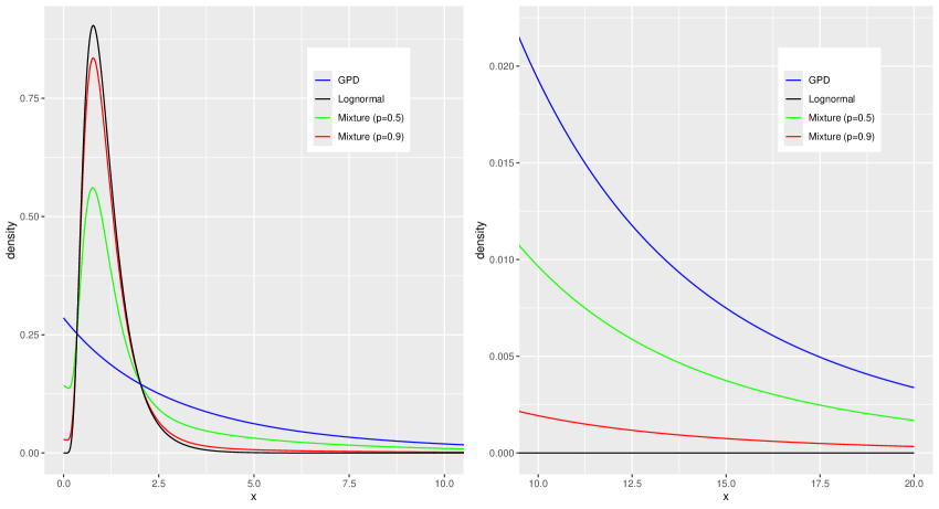
Figure 1: Densities of static lognormal-GPD mixtures with $p\in\{0.9,0.5\}$, $\mu=0$, $\sigma^{2}=0.25$, $\xi=0.25$ and $\beta=3.5$, as well as of the lognormal and GPD component densities. The left panel shows the body ($x\leq 10$), the right panel displays the tail ($x>10$).

From the figure, we notice a few interesting features. First, the GPD is unlikely to be a good model for the bulk of the data: this is not surprising, because the GPD with $\xi>0$ typically fits well only the observations above a high threshold; see, e.g., Embrechts et al., (1997). Second, the GPD tail is heavier than the lognormal one, hence the GPD contribution is key to model the largest observations. Third, the mixture combines the good fit of the lognormal to the body and of the GPD to the extreme observations, and the numerical value of $p$ allows one to obtain a distribution with a specific degree of tail heaviness.

In the present paper we investigate two main issues. The first one is estimation: the implementation and performance of the EM algorithm need to be assessed. The second one is flexibility: is the proposed model sufficiently flexible for data from different skewed and leptokurtic data-generating processes?

The novelty of the paper is twofold. We propose a new model that combines a classical size distribution and a Pareto-type tail, yet remains unsupervised. This implies that, unlike most proposals in the literature, there is no threshold between the two distributions, whose estimation is typically difficult. In a second step we develop an EM algorithm for MLE, which is computationally cheaper than the computer-intensive approaches often necessary in similar setups. All in all, the model is flexible and easy to interpret, while the estimation procedure is reliable and reasonably fast.

The rest of the paper is organized as follows. In Section 2 we give some background about the problem of modeling skewed non-negative data; in Section 3 we introduce the static lognormal-GPD distribution and detail the EM algorithm; in Section 4 we illustrate the outcomes of simulation experiments in correctly- and mis-specified setups; in Section 5 we fit the model to automobile claims data. Finally, in Section 6 we discuss the results and conclude.

2 Background

The literature about models that “combine”, in ways that will be made more precise later, different distributions for the body and the tail is rather rich.

A popular way of proceeding is based on splicing. A two-component spliced distribution is defined by the following density (Panjer,, 2006):

$$f(x)=\begin{cases}a_{1}f_{1}(x),&c_{0}<x<c_{1},\\ a_{2}f_{2}(x),&c_{1}<x<c_{2},\end{cases}$$

where $a_{1},a_{2}>0$, $a_{1}+a_{2}=1$, $f_{1},f_{2}$ are density functions, and the definition can be extended in an obvious way to a finite number of components $k>2$. The family includes various different models, depending not only on the distributions used for the body and the tail, but also on the requirements about the junction point: the resulting density may be discontinuous, continuous or continuous and differentiable. The last two cases require constraints that reduce the number of free parameters.

Second, a closely related model is the dynamic mixture by Frigessi et al., (2002), which has the advantage of a smooth density with no need of finding a threshold, but is characterized by more complicated inferential procedures.

A special version of a spliced model that is also unsupervised, i.e. automatically determines the threshold, has been recently developed in a series of papers (see Dacorogna et al.,, 2023, and the references therein) and is mainly aimed at cyber risk modeling. The idea is to join a lognormal and a GPD via a “bridge” distribution, which is chosen to be an exponential distribution. Continuity and differentiability constraints are used, so that the total number of free parameters is four, and estimation is carried out by means of an iterative algorithm.

Finally, in the actuarial setup, other mixture and spliced models have been proposed for skewed, heavy-tailed and censored or truncated losses: see, e.g., Reynkens et al., (2017), Blostein and Miljkovic, (2019), and Bae and Miljkovic, (2024).

In the rest of the paper, we will compare (2) to two specific cases, namely the composite lognormal-Pareto distribution (Scollnik,, 2007), termed Case 1 in the following, and the Cauchy-lognormal-GPD dynamic mixture (Frigessi et al.,, 2002), called Case 2 from now on. In particular, for these three distributions we will consider modeling capabilities, statistical properties of parameter estimation procedures, and computational costs.

2.1 Case 1: the composite lognormal-Pareto distribution

The continuous and differentiable composite lognormal-Pareto density (Scollnik,, 2007) is given by

$$f(x)=rf_{1}(x;\mu,\sigma^{2},x_{min})+(1-r)f_{2}(x;x_{min},\alpha),$$ (3)

where

$$f_{1}(x;\mu,\sigma^{2},x_{min})=\frac{1}{\Phi\left(\frac{\log(x_{min})-\mu}{\sigma}\right)}\frac{1}{x\sigma\sqrt{2\pi}}e^{-\frac{1}{2}\left(\frac{\log(x)-\mu}{\sigma}\right)^{2}}\mathbb{I}_{\{0<x\leq x_{min}\}}$$ (4)

is the $\text{Logn}(\mu,\sigma^{2})$ density right-truncated at $x_{min}$ and $f_{2}(x;x_{min},\alpha)$ is the Pareto density with scale and shape parameters $x_{min}$ and $\alpha$, respectively. From the definition of the density, we see that this is a spliced distribution. Due to the continuity and differentiability constraints, $r$ and $\mu$ are given by

$$r(\sigma^{2},\alpha) =\frac{\sqrt{2\pi}\alpha\sigma\Phi(\alpha\sigma)e^{\frac{1}{2}(\alpha\sigma)^{2}}}{\sqrt{2\pi}\alpha\sigma\Phi(\alpha\sigma)e^{\frac{1}{2}(\alpha\sigma)^{2}}+1},$$

$$\mu(x_{min},\alpha,\sigma^{2}) =\log(x_{min})-\alpha\sigma^{2}.$$

Therefore, only $\sigma^{2}$, $\alpha$ and $x_{min}$ are free parameters.

2.2 Case 2: the Cauchy-lognormal-GPD dynamic mixture

The density is given by

$$f(x;\boldsymbol{\theta})=\frac{(1-p(x;\mu_{c},\tau))f_{1}(x;\mu,\sigma^{2})+p(x;\mu_{c},\tau)f_{2}(x;\beta,\xi)}{Z},$$ (5)

where $x\in\mathbb{R}^{+}$, $\mu_{c},\mu\in\mathbb{R}$, $\tau,\sigma^{2},\xi,\beta\in\mathbb{R}^{+}$, $\boldsymbol{\theta}=(\mu_{c},\tau,\mu,\sigma^{2},\beta,\xi)^{\prime}$, $f_{1}(x;\mu,\sigma^{2})$ is the lognormal density with parameters $\mu$ and $\sigma^{2}$, $f_{2}(x;\beta,\xi)$ is the zero-location GPD density with scale and shape parameters equal to $\beta$ and $\xi$, respectively. The normalizing constant $Z$ cannot be computed in closed form: it is equal to (for details see Bee,, 2023)

$$Z=Z(\boldsymbol{\theta})=1+\frac{1}{\pi}I,$$

where

$$I=\bigintsss_{0}^{\infty}\left[\frac{1}{\beta}\left(1+\frac{\xi x}{\beta}\right)^{-1/\xi-1}-\frac{1}{\sqrt{2\pi}\sigma x}e^{-\frac{1}{2}\left(\frac{\log{x}-\mu}{\sigma}\right)^{2}}\right]\arctan\left(\frac{x-\mu_{c}}{\tau}\right)dx.$$

The original version of this model, with the lognormal density replaced by the Weibull, had been developed by Frigessi et al., (2002) and was also characterized by the normalizing constant issue.

3 A static lognormal-GPD mixture

In the present paper we implement the EM algorithm for MLE of the finite mixture with density (1). In the following we will call it a static mixture, to avoid confusion with the dynamic mixture of Section 2.2. As usual in finite mixture analysis (e.g., McLachlan and Peel,, 2000), MLE would be easy if population membership were known, and we are now going to exploit this feature to implement the EM algorithm.

3.1 Maximum Likelihood Estimation: the EM algorithm

Let $\boldsymbol{x}=(x_{1},\dots,x_{n})$ be the observed data, i.e., a random sample from a mixture distribution. Let $\boldsymbol{z}=(z_{1j},\dots,z_{nj})$ represent the missing data, with $z_{ij}$ ($i=1,\dots,n$) being an indicator variable of population membership: $z_{ij}=1$ if the $i$-th observation belongs to the $j$-th population, and $z_{ij}=0$ otherwise. Let $\ell(\boldsymbol{\theta})$ be the observed log-likelihood function obtained from the mixture density, with $\boldsymbol{\theta}\in\boldsymbol{\Theta}\subset\mathbb{R}^{d}$ a vector of parameters. Let $\boldsymbol{v}=(\boldsymbol{x}^{\prime},\boldsymbol{z}^{\prime})^{\prime}$ be the complete data, with density and complete log-likelihood denoted by $g_{c}(\boldsymbol{v};\boldsymbol{\theta})$ and $\ell_{c}(\boldsymbol{\theta})$ respectively. At the $t$-th iteration, the algorithm is carried out by means of two steps.

E-step. Compute the conditional expectation of $\ell_{c}(\boldsymbol{\theta})$, given the current value of $\boldsymbol{\theta}$ and the observed sample $\boldsymbol{x}$:

$$Q(\boldsymbol{\theta};\boldsymbol{\theta}^{(t)})\stackrel{{\scriptstyle\text{def}}}{{=}}\text{E}_{\boldsymbol{\theta}^{(t)}}\{\ell_{c}(\boldsymbol{\theta})|\boldsymbol{x}\}.$$ (6)

M-step. Maximize, with respect to $\boldsymbol{\theta}$, the so-called $Q$-function, i.e. the conditional expectation of $\ell_{c}(\boldsymbol{\theta})$ provided by the E-step (6):

$$\boldsymbol{\theta}^{(t+1)}=\operatorname*{arg\,max}_{\boldsymbol{\theta}}Q(\boldsymbol{\theta};\boldsymbol{\theta}^{(t)}).$$ (7)

The E- and M-step (6) and (7) are then iterated until convergence is reached according to some stopping rule. The algorithm monotonically increases the observed likelihood at each iteration; under regularity conditions (Wu,, 1983), the sequence $\boldsymbol{\theta}^{(t)}$ converges to a stationary point and the estimators are asymptotically efficient.

Let us now turn to the present setup: let $\boldsymbol{x}=(x_{1},\dots,x_{n})$ be the observed data, i.e., a random sample from the static lognormal-GPD mixture (2). Let $\boldsymbol{z}=(z_{1},\dots,z_{n})$ represent the missing data, with $z_{i}=1$ if the $i$-th observation is lognormal, and $z_{i}=0$ if it is GPD. The observed and complete log-likelihood functions are respectively equal to:

$$\ell(\boldsymbol{\theta};\boldsymbol{x}) =\sum_{i=1}^{n}\log\{pf_{1}(x;_{i}\mu,\sigma^{2})+(1-p)f_{2}(x_{i};\xi,\beta)\},$$

$$\ell_{c}(\boldsymbol{\theta};\boldsymbol{x},\boldsymbol{z}) =\sum_{i=1}^{n}z_{i}\log f_{1}(x_{i};\mu,\sigma^{2})+\sum_{i=1}^{n}(1-z_{i})\log f_{2}(x_{i};\xi,\beta).$$

The conditional expectation of the complete log-likelihood function is given by

$$\text{E}(\ell_{c}(\boldsymbol{\theta};\boldsymbol{x})|\boldsymbol{x},\boldsymbol{\theta}^{(t)})=\sum_{i=1}^{n}\tau_{i1}^{(t)}\log f_{1}(x;_{i}\mu^{(t)},\eta^{(t)})+\sum_{i=1}^{n}\tau_{2i}^{(t)}\log f_{2}(x_{i};\xi^{(t)},\beta^{(t)}),$$ (8)

where $\eta\stackrel{{\scriptstyle\text{def}}}{{=}}\sigma^{2}$, $\tau_{2i}^{(t)}=1-\tau_{i1}^{(t)}$ and

$$\tau_{i1}^{(t)}=\frac{p^{(t)}f_{1}(x_{i};\mu^{(t)},\eta^{(t)})}{p^{(t)}f_{1}(x_{i};\mu^{(t)},\eta^{(t)})+(1-p^{(t)})f_{2}(x_{i};\xi^{(t)},\beta^{(t)})}.$$ (9)

Equation (9), which is the E-step of the algorithm, represents the posterior probability, at the $t$-th iteration, that the $i$-tho observation belongs to the lognormal population. At convergence, this quantity can be used for classification purposes.

As for the M-step, it results from the maximization of (8) with respect to all parameters. The M-steps for $p$, $\mu$ and $\eta$ are given in closed form by

$$p^{(t)} =\frac{1}{n}\sum_{i=1}^{n}\tau_{i1}^{(t)};$$

$$\mu^{(t)} =\frac{1}{np^{(t)}}\sum_{i=1}^{n}\tau_{i1}^{(t)}\log x_{i};$$

$$\eta^{(t)} =\frac{1}{np^{(t)}}\sum_{i=1}^{n}\tau_{i1}^{(t)}(\log x_{i}-\mu^{(t)})^{2}.$$

On the other hand, even in the complete-data case, the MLEs of $\xi$ and $\beta$ can only be found via numerical maximization. Hence, the M-steps for the GPD parameters are not explicit. Specifically, they are the solution of the maximization of the second summand of (8):

$$\xi^{(t)},\beta^{(t)}=\arg\max_{\xi,\beta}\sum_{i=1}^{n}\tau_{2i}\log f_{2}(x_{i};\xi,\beta).$$ (10)

The function $\sum_{i=1}^{n}\tau_{2i}\log f_{2}(x_{i};\xi,\beta)$ is essentially a weighted version of the GPD log-likelihood function and can be maximized analogously, by means of standard optimization routines.

Practical implementation of the algorithm requires specification of initial values $p^{(0)}$, $\mu^{(0)}$, $\eta^{(0)}$, $\xi^{(0)}$ and $\beta^{(0)}$. For the mixing weight we set

$$p^{(0)}=\frac{\#\{y:y<\text{median}(y)\}}{n}.$$

For $\mu^{(0)}$ and $\eta^{(0)}$ we use the lognormal MLEs, whereas $\xi^{(0)}$ and $\beta^{(0)}$ are given by the GPD MLEs, in both cases computed with all the observations.

For the EM algorithm, stopping rules are usually based on subsequent values of either estimated parameters in the M-step, or of maximized log-likelihood. In this paper we use the first approach; in particular, the algorithm stops when $\max_{1\leq i\leq 5}|\theta_{i}^{(t)}-\theta_{i}^{(t-1)}|<\epsilon$, with $\boldsymbol{\theta}=(p,\mu,\eta,\xi,\beta)^{\prime}$ and $\epsilon=10^{-6}$.

4 Simulation experiments

The experiments in this section have a twofold goal. First, we aim at assessing the finite-sample behavior of the estimators in the correctly-specified setup. Second, we sample from the data-generating processes (DGPs) of Case 1 and 2 and compare the static mixture with the two models (3) and (5); in other words, we estimate our model in a mis-specified setup, to study the properties of parameter and Value-at-Risk (VaR) estimators.

4.1 Correctly-specified setup

We simulate observations from (2) with $p=0.9$, $\mu=0$, $\sigma^{2}=0.25$, $\xi\in\{0.25,0.5\}$, $\beta=3.5$, for sample sizes $n\in\{100,500\}$. For the case $\xi=0.5$, the simulated distributions of the EM-based estimators $\hat{p}$, $\hat{\xi}$ and $\hat{\beta}$ are shown in Figure 2. The number of replications is $B=1000$. As can be seen, the properties of the estimators considerably improve when $n=500$: the variance is smaller, there are fewer outliers and the distributions of $\hat{p}$ and $\hat{\xi}$ are more “bell-shaped”.

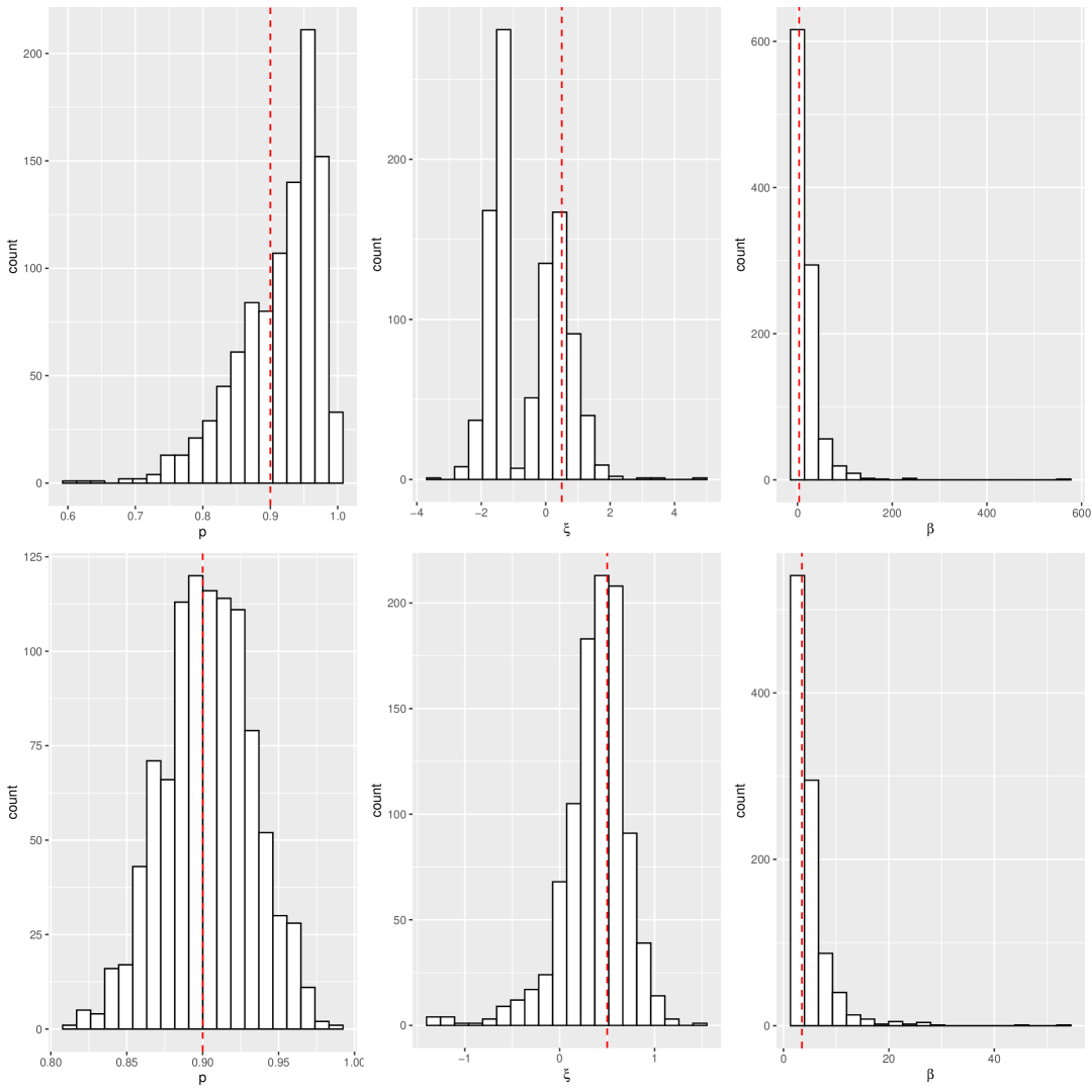
Figure 2: Histogram of the simulated distributions of the estimators for $n=100$ (first row) and $n=500$ (second row) in the correctly-specified setup. The red vertical lines represent the true values of the parameters.

Table 1 shows the bias and median-bias of the estimators, Table 2 displays the root-mean-squared-error (RMSE) along with the median-RMSE (RMSE_med). Letting $\tilde{\theta}_{i}=\text{median}_{j=1,\dots,B}\theta_{i,j}$ ($i=1,\dots,d$), where $\theta_{i,j}$ are the $B$ simulated values of the $i$-th parameter, the median-RMSE is given by

$$RMSE_{med}(\hat{\theta}_{i})=\sqrt{b_{med}(\theta_{i})^{2}+mad(\theta_{i})^{2}},$$

where $b_{med}(\theta_{i})\stackrel{{\scriptstyle\text{def}}}{{=}}\tilde{\theta}_{i}-\theta_{i}$ and $mad(\theta_{i})\stackrel{{\scriptstyle\text{def}}}{{=}}\text{median}_{j=1,\dots,B}|\theta_{i,j}-\tilde{\theta}_{i}|$ are the median-bias and the median absolute deviation, respectively. The reason why we also compute median-based accuracy measures is their robustness to outliers. In all tables, the true values of $\mu$ and $\sigma$ are $\mu=0$ and $\sigma=0.5$.

Table 1: Bias and median-bias when $p=0.9$, $\xi=0.5$ and $\beta=3.5$.

		$p$	$\mu$	$\sigma$	$\xi$	$\beta$
$n=100$	bias	0.013	0.005	0.000	$-1.053$	14.515
	bmed	0.030	0.004	0.002	$-1.563$	5.611
$n=500$	bias	$-0.003$	$-0.002$	$-0.000$	0.127	$-1.390$
	bmed	0.004	0.002	0.000	$-0.087$	0.350

Table 2: RMSE and RMSE_med when $p=0.9$, $\xi=0.5$ and $\beta=3.5$.

		$p$	$\mu$	$\sigma$	$\xi$	$\beta$
$n=100$	RMSE	0.063	0.060	0.054	1.509	32.702
	RMSEmed	0.061	0.060	0.051	2.008	11.788
$n=500$	RMSE	0.001	0.001	0.001	0.133	16.801
	RMSEmed	0.030	0.026	0.024	0.287	1.675

While for $n=500$ the median-based bias and RMSE show no obvious changes with respect to the corresponding mean-based measures, when $n=100$ there are considerable differences, in line with the outliers noted in Figure 2. This suggests that, for small sample size, the algorithm sometimes does not converge; notice that this issue mostly affects the GPD parameters.

4.2 Mis-specified models

The outcomes of the previous section suggest that the EM-based fitting procedure of the static lognormal-GPD distribution is effective in a correctly-specified setup. To check whether the model is suitable also for other DGPs, in this section we study its goodness of fit when the true distribution is different from (2). In particular, we fit the model to data from the composite lognormal-Pareto distribution developed by Scollnik, (2007), termed Case 1 in Section 2, and the Cauchy-lognormal-GPD dynamic mixture proposed by Frigessi et al., (2002), called Case 2 in Section 2.

4.2.1 Case 1: the composite lognormal-Pareto distribution

Figure 3 displays the histogram of 500 observations sampled from the composite distribution of Case 1, with parameters $\mu=0$, $\sigma=0.5$, $x_{min}=5$ and $\alpha=2$. The true density and the estimated static mixture with parameters equal to the mean of the 1000 estimated parameter vectors obtained in the simulation experiments are displayed as well.

Table 3 (when $\alpha=2$) and Table 4 (when $\alpha=1.5$) show parameter estimates and standard errors; in addition, we report the p-values of the Kolmogorov-Smirnov (KS) and Anderson-Darling (AD) goodness-of-fit (GoF) tests.

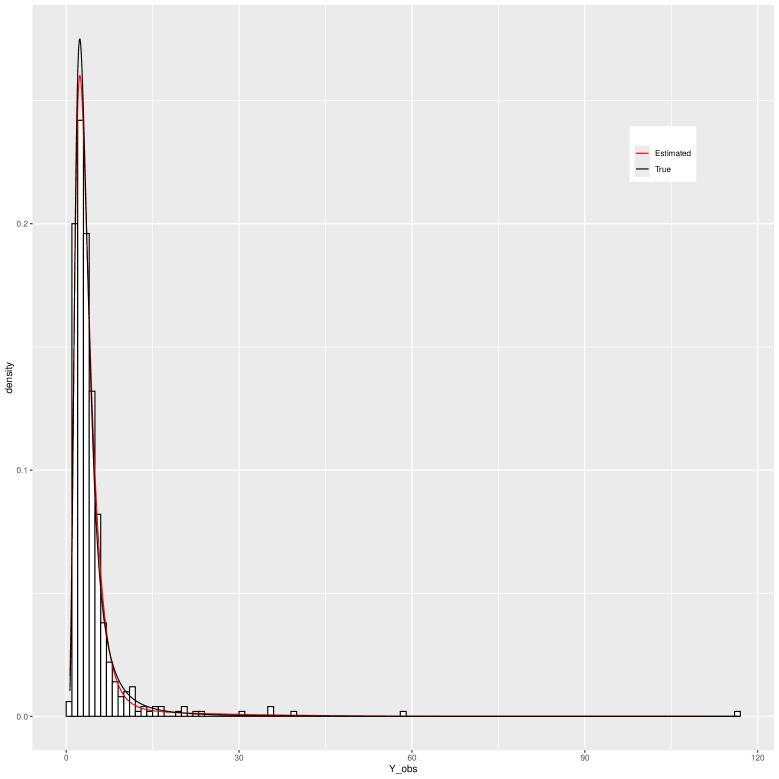
Figure 3: Histogram of the simulated data from Case 1 ($n=500$, $\mu=0$, $\sigma=.5$, $x_{min}=5$ and $\alpha=2$), along with the true density and the estimated lognormal-GPD static density.

Table 3: Case 1: parameter estimates, standard errors and p-values of the GoF tests for Case 1 with $\mu=0$, $\sigma=0.5$, $x_{min}=5$ and $\alpha=2$.

	$p$	$\mu$	$\sigma$	$\xi$	$\beta$	KS	AD
$n=100$	0.943	1.162	0.537	$-0.918$	42.254	0.657	0.643
	(0.061)	(0.058)	(0.064)	(0.772)	(78.148)	(0.254)	(0.254)
$n=500$	0.933	1.147	0.528	$-0.181$	20.046	0.593	0.564
	(0.028)	(0.025)	(0.026)	(0.441)	(18.203)	(0.265)	(0.251)

Table 4: Case 1: parameter estimates, standard errors and p-values of the GoF tests with $\mu=0$, $\sigma=0.5$, $x_{min}=5$ and $\alpha=1.5$.

	$p$	$\mu$	$\sigma$	$\xi$	$\beta$	KS	AD
$n=100$	0.895	1.327	0.563	$-0.545$	87.531	0.638	0.620
	(0.082)	(0.073)	(0.079)	(0.815)	(780.324)	(0.272)	(0.259)
$n=500$	0.875	1.307	0.549	0.194	19.285	0.551	0.494
	(0.037)	(0.029)	(0.030)	(0.246)	(9.088)	(0.261)	(0.242)

As of parameter estimates, the standard deviation of $\hat{\beta}$ when $n=100$ is noticeably large. Nevertheless, both Figure 3 and the GoF tests in tables 3 and 4 suggest that the fit is excellent.

Since these kinds of distributions are expected to be especially important for risk measurement purposes, Table 5 displays the estimated VaR obtained via the correctly-specified model and the mis-specified lognormal-GPD distribution, along with the true quantile. The VaR is computed via Monte Carlo simulation with $10^{4}$ replications. 95% confidence intervals are reported as well. The point estimates of the VaRs are close to each other and, as clearly results from the confidence intervals, they are not significantly different from each other.

Table 5: Case 1: estimated VaR when $\sigma=.5$, $\xi=2$, $x_{min}=5$; 95% confidence intervals are in brackets.

		0.95	0.99	0.995
$n=100$	Correct-spec.	10.953	25.378	36.594
		[8.349,14.534]	[13.688,43.223]	[16.970,68.417]
	Misspec.	10.877	27.444	34.921
		[8.144,17.683]	[12.155,73.428]	[13.408,114.102]
$n=500$	Correct-spec.	10.605	23.801	33.679
		[9.291,11.986]	[18.104,30.524]	[23.954,44.842]
	Misspec.	9.968	27.682	37.911
		[8.664,12.228]	[16.303,42.868]	[20.867.62.658]
True		10.568	23.630	33.346

4.2.2 Case 2: the Cauchy-lognormal-GPD dynamic mixture

We perform the same analysis of Section 4.2.1 when the true DGP is the Cauchy-lognornal-GDP distribution (Case 2 in Section 2). Figure 4 displays the histogram of 500 observations sampled from the dynamic mixture with parameters $\mu_{c}=1$, $\tau=2$, $\mu=0$, $\sigma^{2}=0.25$, $\xi=0.25$ and $\beta=3.5$. Superimposed to the histogram are the true density and the estimated static mixture with parameters equal to the mean of the 1000 estimated parameter vectors obtained in the simulation experiments.

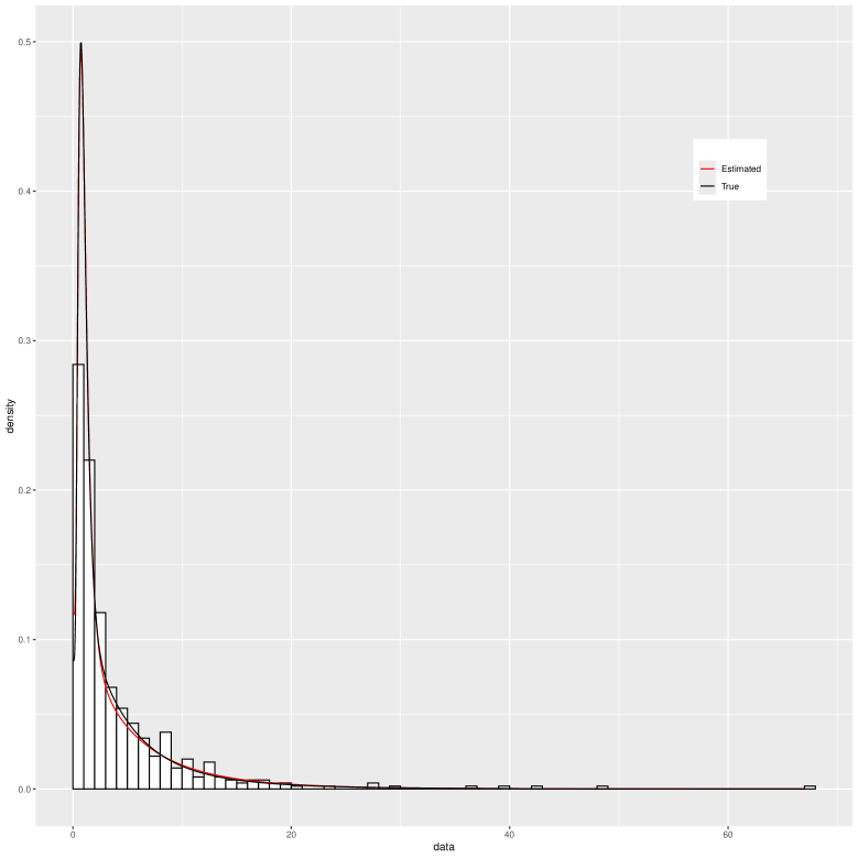
Figure 4: Histogram of the simulated data from Case 2 ($n=500$, $\mu_{c}=1$, $\tau=2$, $\mu=0$, $\sigma^{2}=0.25$, $\xi=0.25$ and $\beta=3.5$) along with the true density and the estimated lognormal-GPD static density.

Tables 6 and 7 display parameter estimates, standard errors and $p$-values of the GoF tests for Case 2 when $\xi=0.25$ and $\xi=0.5$, respectively. The tests confirm that the static lognormal-GPD fits quite well the data: Table 8 reports the correctly-specified VaR, computed using the dynamic mixture with parameters estimated via MLE, and the mis-specified VaR estimated from the static mixture, with corresponding standard errors.

Table 6: Case 2: parameter estimates, standard errors and p-values of the GoF tests for Case 2 with $\mu_{c}=1$, $\tau=2$, $\mu=0$, $\sigma^{2}=0.25$, $\xi=0.25$ and $\beta=3.5$.

	$\pi$	$\mu$	$\sigma$	$\xi$	$\beta$	KS	AD
$n=100$	0.442	$-0.017$	0.488	$-0.001$	7.188	0.690	0.673
	(0.152)	(0.176)	(0.165)	(0.363)	(9.278)	(0.253)	(0.253)
$n=500$	0.403	$-0.048$	0.480	0.131	5.002	0.653	0.626
	(0.053)	(0.063)	(0.060)	(0.075)	(0.603)	(0.264)	(0.272)

Table 7: Case 2: parameter estimates, standard errors and p-values of the GoF tests for Case 2 with $\mu_{c}=1$, $\tau=2$, $\mu=0$, $\sigma^{2}=0.25$, $\xi=0.5$ and $\beta=3.5$.

	$\pi$	$\mu$	$\sigma$	$\xi$	$\beta$	KS	AD
$n=100$	0.434	$-0.0188$	0.492	0.275	7.963	0.675	0.674
	(0.140)	(0.178)	(0.163)	(0.350)	(15.937)	(0.255)	(0.249)
$n=500$	0.398	$-0.051$	0.477	0.381	5.312	0.642	0.628
	(0.050)	(0.060)	(0.058)	(0.087)	(0.713)	(0.257)	(0.258)

Table 8: Case 2: estimated VaR with $\mu_{c}=1$, $\tau=2$, $\mu=0$, $\sigma^{2}=0.25$, $\xi=0.25$ and $\beta=3.5$. 95% confidence intervals are in brackets.

		0.95	0.99	0.995
$n=100$	Correct-spec.	14.218	29.056	38.241
		[9.665,20.191]	[16.831,54.053]	[20.023,79.467]
	Misspec.	14.549	26.604	32.613
		[10.121,20.035]	[14.497,44.409]	[15.975,58.978]
$n=500$	Correct-spec.	14.262	28.694	37.028
		[12.101,16.144]	[21.716,37.209]	[26.199,51.662]
	Misspec.	14.602	27.146	33.479
		[12.445,17.081]	[21.414,35.180]	[25.055.44.737]
True		14.211	28.352	36.342

The estimated VaRs are again very close to each other, and the differences are non-significant, as shown by the large overlap of the confidence intervals. In this setup, unlike Case 1, the static mixture has narrower confidence intervals, presumably because the dynamic mixture has one parameter more, and overall its estimation is difficult.

4.3 Computing times

To assess the computational burden of the three approaches, we sample and estimate each of the three models considered so far, i.e. the static lognormal-GPD mixture, the composite lognormal-Pareto (Case 1) and the dynamic lognormal-GPD (Case 2). Notice that the three methods are always used in the correctly-specified setup. In all cases, the sample size is $n=500$.

The average computing times (in seconds) based on 1000 replications are as follows:

• 0.145 for the static EM with true parameter values $p=0.9$, $\mu=0$, $\sigma=0.5$, $\xi=0.5$, $\beta=3.5$;

• 0.015 for the composite lognormal-Pareto distribution (Case 1) with parameters $\sigma=0.5$, $\alpha=2$, $x_{min}=5$;

• 40.96 for the Cauchy-lognormal-GPD dynamic mixture (Case 2), with true parameter values $\mu_{c}=1$, $\tau=2$, $\mu=0$, $\sigma=0.5$, $\xi=0.5$, $\beta=3.5$.

The EM-based approach is not as fast as MLE estimation of the lognormal-Pareto distribution, which is not surprising, given that the EM algorithm is known to be rather slow (see, e.g., McLachlan and Krishnan,, 2008, Section 3.9). However, it is much faster than MLE in Case 2.

5 Empirical analysis

In this section we analyze the distribution of claims experience from a large midwestern (US) property and casualty insurer for private passenger automobile insurance. The data are the amounts, in US dollars, paid on closed claims, and are publicly available in the AutoClaims dataset of the R package insuranceData. The sample size is $n=6773$.

The upper panel of Figure 5 shows the histogram of the data with superimposed the estimated static density: the fit looks quite good. Further support comes from Table 9, which reports average $p$-values of the KS and AD tests for the mixture as well as for the pure lognormal and GPD: the GoF tests confirm that the estimated density is an appropriate model for the data.

Table 9: Average $p$-value of the KS and AD tests for the estimated mixture, lognormal and GPD.

	Mixture	Lognormal	GPD
KS	0.787	0.044	$<0.001$
AD	0.829	0.021	$<0.001$

The middle and bottom panels of Figure 5 display the body and the tail of the estimated densities, as well as the lognormal and GPD densities estimated using all the observations. The latter is not a good fit to the smallest observations, a feature that is commonly observed for the GPD with $\xi>0$. For data in this range, the lognormal provides a better fit, and so does the mixture, because most observations are lognormal, as made clear by the posterior probabilities in Figure 6. On the other hand, due to theoretical results in extreme value theory, the GPD is assumed to be best at modeling the tail, and the mixture gets closer and closer to the GPD when we consider larger observations.

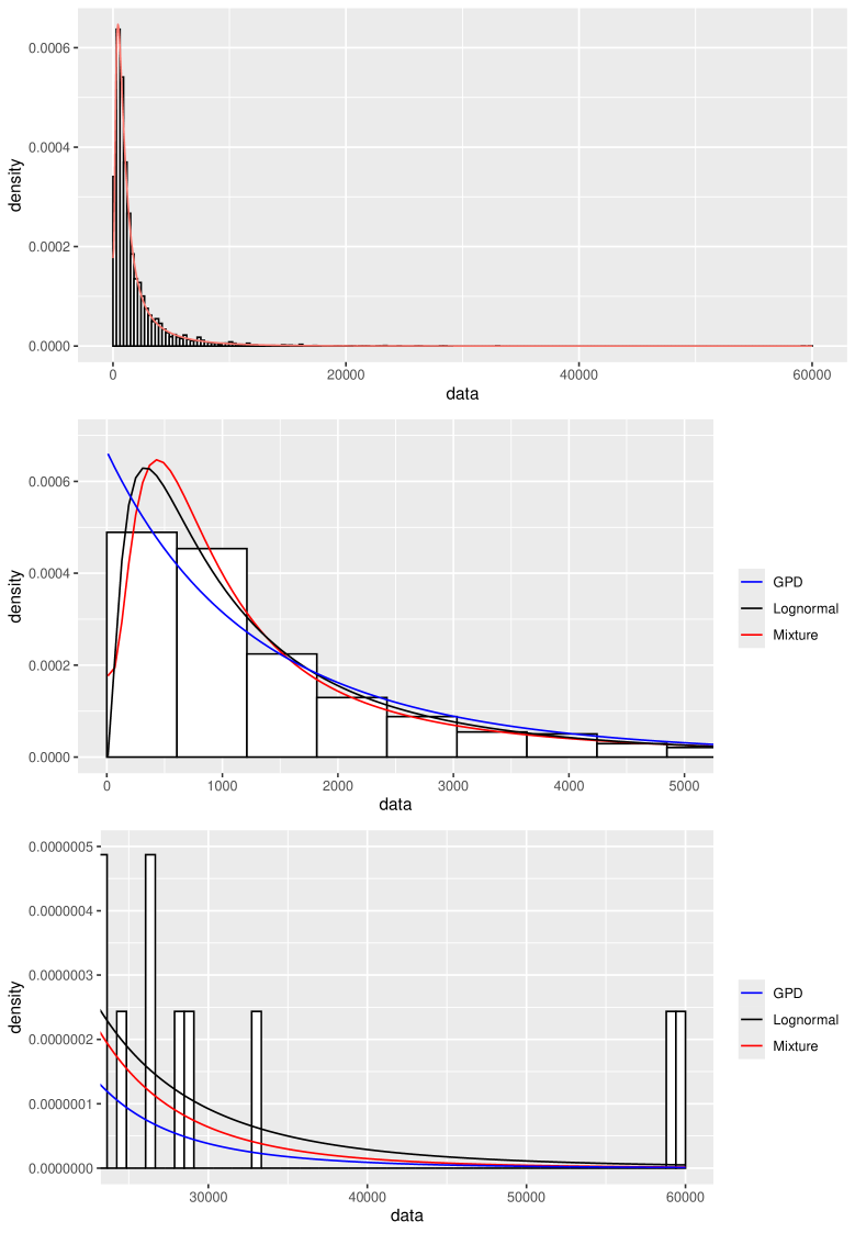
Figure 5: Top panel: histogram of the AutoClaims data, with superimposed the lognormal-GPD density. Middle panel: zoom on the distribution body ($x<5000$). Bottom panel: zoom on the distribution tail ($x>25\,000$). In the last two panels, the estimated lognormal and GPD densities are shown as well.

Table 10 reports parameter estimates, bootstrap standard errors based on 1000 replications, and 95% confidence intervals. The outcomes imply an heavy-tailed distribution, since $\hat{\xi}>0$. The confidence intervals suggest a high precision: for example, the interval for $\xi$ goes from 0.102 to 0.205, thus confirming that the data are heavy-tailed.

Table 10: Parameter estimates, bootstrap standard errors and 95% confidence intervals in the AutoClaims example.

$p$	$\mu$	$\sigma$	$\xi$	$\beta$
0.567	6.676	0.752	0.156	2442.700
(0.038)	(0.030)	(0.034)	(0.028)	(125.422)
$[0.499,0.645]$	$[6.618,6.735]$	$[0.688,0.820]$	$[0.102,0.205]$	$[2240.414,2725.608]$

Figure 6 is a scatterplot of the observations versus the posterior probabilities of belonging to the lognormal distribution, $\tau_{i1}$.

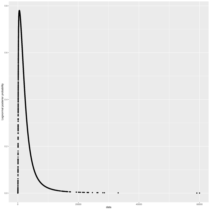
Figure 6: Scatterplot of the observations versus the posterior probabilities of belonging to the lognormal distribution, $\tau_{i1}$.

For the bulk of the data, the posterior probability takes intermediate values, so that both distributions are likely to have generated them. In particular, for all the observations between $x_{(172)}$ and $x_{(5339)}$, $\tau_{i1}\in[0.40,0.780]$, where 0.780 is the largest value of $\tau_{i1}$ for this dataset. On the other hand, the largest observations belong to the GPD with probability very close to 1: the top 50 observations have $\tau_{i2}>0.99$, that is, are very likely to be generated by the GPD. This suggests that the model works well also for classification purposes.

Finally, we estimate VaR at three different levels. To assess variability, the VaR is recomputed with the estimated parameter values obtained in the 1000 non-parametric bootstrap replications employed for the bootstrap analysis in Table 10.

Table 11: VaR estimates, bootstrap standard errors and 95% confidence intervals in the AutoClaims example. For comparison purposes, the last line reports the quantiles of the observed data.

	$\alpha=95\%$	$\alpha=99\%$	$\alpha=99.5\%$
Static	6382.85	12 540.60	15 698.36
	(222.87)	(682.73)	(1082.96)
	$[5950.74,6834.79]$	$[11\,250.84,13\,952.80]$	$[13\,633.93,17\,959.04]$
Case 1	6810.63	15 048.99	20 426.43
	(545.06)	(1906.43)	(3226.70)
	$[5862.78,7967.64]$	$[11\,715.95,19\,227.58]$	$[15\,039.30,27\,668.46]$
Case 2	5470.00	11 459.60	15 036.81
	(590.60)	(1587.31)	(2391.44)
	$[4896.07,6875.40]$	$[9714.15,15\,383.81]$	$[12\,303.07,21\,210.88]$
True	6737.81	12 713.65	15 024.10

From Table 11 we see that the static lognormal-GPD mixture and the dynamic Cauchy-lognormal-GPD mixture (Case 2) yield similar measures, but the former is more precise at high levels, as can be seen by comparing the estimated standard deviations and the width of the confidence intervals. Notice also that both methods yield VaR mesures in line with the corresponding quantiles of the observed data. On the other hand, the composite lognormal-Pareto distribution (Case 1) not only gives higher VaR estimates, but also a larger variability.

6 Conclusion

In this paper we have proposed a flexible unsupervised lognormal-GPD mixture for skewed and heavy-tailed distribution. A maximum likelihood estimation procedure based on the EM algorithm is developed and its properties are studied via simulation experiments.

With respect to competing models, the advantages range from an easy interpretation to a reliable estimation procedure characterized by a low computational burden. Unlike the lognormal-Pareto composite model developed by Scollnik, (2007), the density is always continuous, without the need of constraints; with respect to the dynamic mixture proposed by Frigessi et al., (2002), the density is normalized, so that it is not necessary to tackle the additional problem of evaluating the normalization constant.

In terms of flexibility, the static lognormal-GPD distribution yields excellent results when used for fitting data in mis-specified setups, and allows the investigator to estimate VaR measures quite precisely. In particular, the VaR computed via the static lognormal-GPD model is less variable than via the lognormal-GPD dynamic mixture.

In principle, the proposed approach may be extended to the case of left-censored (or truncated) data. In such a setup, the M-steps for the lognormal parameters would not be in closed form either, but it should be possible to use a nested EM-algorithm (van Dyk,, 2000): at the $t$-th iteration of the EM algorithm presented in Section 3.1, the lognormal parameters are estimated by means of an EM algorithm for MLE of the censored or truncated lognormal distribution (Bee,, 2006).

Even though the main purpose of this paper is the development and estimation of a model for skewed and heavy-tailed data, there are setups where classification is the main purpose, i.e. where the main goal is identifying which observations are lognormal and which are GPD. Since one of the byproducts of the EM algorithm are posterior probability of the observations, our approach is very well suited also for this aim.

References

- Axtell, (2001) Axtell, R. L. (2001). Zipf distribution of U.S. firm sizes. Science, 293(5536):1818–1820.
- Bae and Miljkovic, (2024) Bae, T. and Miljkovic, T. (2024). Loss modeling with the size-biased lognormal mixture and the entropy regularized EM algorithm. Insurance: Mathematics and Economics, 117:182–195.
- Bee, (2006) Bee, M. (2006). Estimating the parameters in the loss distribution approach: How can we deal with truncated data? In Davis, E., editor, The Advanced Measurement Approach to Operational Risk, pages 123–144. Risk Books.
- Bee, (2023) Bee, M. (2023). Unsupervised mixture estimation via approximate maximum likelihood based on the Cramér - von Mises distance. Computational Statistics & Data Analysis, 185:107764.
- Bee et al., (2011) Bee, M., Riccaboni, M., and Schiavo, S. (2011). Pareto versus lognormal: A maximum entropy test. Physical Review E, 84:026104.
- Blostein and Miljkovic, (2019) Blostein, M. and Miljkovic, T. (2019). On modeling left-truncated loss data using mixtures of distributions. Insurance: Mathematics and Economics, 85:35–46.
- Cruz et al., (2015) Cruz, M., Peters, G., and Shevchenko, P. (2015). Fundamental Aspects of Operational Risk and Insurance Analytics: A Handbook of Operational Risk. Wiley.
- D’Acci, (2019) D’Acci, L. (2019). The Mathematics of Urban Morphology. Birkhäuser.
- Dacorogna et al., (2023) Dacorogna, M., Debbabi, N., and Kratz, M. (2023). Building up cyber resilience by better grasping cyber risk via a new algorithm for modelling heavy-tailed data. European Journal of Operational Research, 311(2):708–729.
- Embrechts et al., (1997) Embrechts, P., Klüppelberg, C., and Mikosch, T. (1997). Modelling Extremal Events for Insurance and Finance. Springer.
- Frigessi et al., (2002) Frigessi, A., Haug, O., and Rue, H. (2002). A dynamic mixture model for unsupervised tail estimation without threshold selection. Extremes, 3(5):219–235.
- Goerlich, (2023) Goerlich, F. J. (2023). Income distribution. In Maggino, F., editor, Encyclopedia of Quality of Life and Well-Being Research, pages 3398–3401. Springer International Publishing, Cham.
- Klugman et al., (2019) Klugman, S. A., Panjer, H. H., and Willmot, G. E. (2019). Loss Models: from Data to Decisions. Wiley, 5th edition.
- McLachlan and Krishnan, (2008) McLachlan, G. and Krishnan, T. (2008). The EM Algorithm and Extensions. Wiley, second edition.
- McLachlan and Peel, (2000) McLachlan, G. and Peel, D. (2000). Finite Mixture Models. Wiley.
- McNeil et al., (2015) McNeil, A., Frey, R., and Embrechts, P. (2015). Quantitative Risk Management: Concepts, Techniques, Tools. Princeton University Press, 2nd edition.
- Panjer, (2006) Panjer, H. H. (2006). Operational risk modeling analytics. Wiley.
- Reynkens et al., (2017) Reynkens, T., Verbelen, R., Beirlant, J., and Antonio, K. (2017). Modelling censored losses using splicing: A global fit strategy with mixed Erlang and extreme value distributions. Insurance: Mathematics and Economics, 77:65–77.
- Scollnik, (2007) Scollnik, D. (2007). On composite lognormal-Pareto models. Scandinavian Actuarial Journal, 1:20–33.
- van Dyk, (2000) van Dyk, D. A. (2000). Nesting EM algorithms for computational efficiency. Statistica Sinica, 10(1):203–225.
- Wu, (1983) Wu, C. F. J. (1983). On the convergence properties of the EM algorithm. Annals of Statistics, 11(1):95–103.