Demystifying the Paradox of Importance Sampling with an Estimated History-Dependent Behavior Policy in Off-Policy Evaluation
Abstract
This paper studies off-policy evaluation (OPE) in reinforcement learning with a focus on behavior policy estimation for importance sampling. Prior work has shown empirically that estimating a history-dependent behavior policy can lead to lower mean squared error (MSE) even when the true behavior policy is Markovian. However, the question of why the use of history should lower MSE remains open. In this paper, we theoretically demystify this paradox by deriving a bias-variance decomposition of the MSE of ordinary importance sampling (IS) estimators, demonstrating that history-dependent behavior policy estimation decreases their asymptotic variances while increasing their finite-sample biases. Additionally, as the estimated behavior policy conditions on a longer history, we show a consistent decrease in variance. We extend these findings to a range of other OPE estimators, including the sequential IS estimator, the doubly robust estimator and the marginalized IS estimator, with the behavior policy estimated either parametrically or non-parametrically.
1 Introduction
Off-policy evaluation (OPE) focuses on estimating the average return (sum of discounted rewards) of a specific decision policy, referred to as the target policy, by leveraging historical data collected under a potentially different policy, known as the behavior policy. OPE is vital in numerous domains where direct experimentation is impractical due to high costs, potential risks, or ethical concerns, such as in healthcare (Murphy et al., 2001; Hirano et al., 2003), recommendation systems (Chapelle & Li, 2011) and robotics (Levine et al., 2020).
One widely used OPE method is importance sampling (IS, see e.g., Precup et al., 2000), which employs a reweighting approach to handle the distribution shift between the target policy and the behavior policy. This approach is straightforward: returns generated by the behavior policy are re-weighted based on the ratio of the probability of selecting actions under the target policy to that under the behavior policy. The re-weighted returns are then averaged to produce an unbiased estimator of the target policy’s value. In the limit, as the number of trajectories increases, this estimator converges to the true value of the target policy. However, with finite samples, IS may exhibit high variance, causing considerable estimation error. Consequently, more advanced estimators have been proposed to lower its variance, including the doubly robust (DR) estimator (Jiang & Li, 2016; Thomas & Brunskill, 2016) and marginalized IS estimator (MIS, Liu et al., 2018). Despite its limitation, IS serves as a foundation for many OPE methods and is particularly valued in practice for its unbiasedness. It is also frequently used in off-policy learning algorithms, such as the proximal policy optimization algorithm (Schulman et al., 2017), which is widely used for fine-tuning large language models (Ouyang et al., 2022).
In practice, the behavior policy might be unknown and must be estimated from the historical data to construct the IS ratio. Paradoxically, IS with an estimated behavior policy results in an estimator with lower asymptotic variance and often lower finite-sample mean-squared error (MSE) compared to IS using the true behavior policy. This result has been shown in the statistics (Henmi et al., 2007), causal inference (Hirano et al., 2003; Rosenbaum & Rubin, 1983), multi-armed bandit (Xie et al., 2019a), and Markov decision process (MDP) policy evaluation (Hanna et al., 2021) literature. Furthering the paradox, Hanna et al. showed empirically that in MDPs where the true behavior policy is a first-order Markov-policy (action selection is conditioned only on the current state), the IS estimator’s MSE could be lowered by estimating a higher-order Markov-policy where action selection is conditioned on a history of preceding states (2021). However, the theoretical basis and generality of this finding was left as an open question.
In this work, we establish a comprehensive theoretical framework for analyzing OPE estimators with history-dependent IS ratios; refer to Table 1 for a quick summary of our findings. Our contributions are as follows:
-
•
We demystify the aforementioned paradox for ordinary IS (OIS) estimators with history-dependent IS ratios by deriving a bias-variance decomposition of their MSEs. Our findings reveal that in large samples, the variance component becomes the leading term in the MSE and can be reduced through history-dependent behavior policy estimation. Specifically, increasing the history-length, decreases the variance.
-
•
We also show that there is no free lunch for using history-dependent IS ratios, as it comes at the price of increasing the bias of the resulting OPE estimator, which becomes non-negligible in finite samples.
-
•
We extend these findings to accommodate other variants of IS estimators, including the sequential IS (SIS), DR and MIS estimators, with the behavior policy estimated either parametrically, or non-parametrically. Interestingly, incorporating history-dependent IS ratios has different effects on the asymptotic variances of these estimators:
-
(1)
It reduces the asymptotic variance for SIS;
-
(2)
It leaves the asymptotic variance of DR unchanged when the Q-function is correctly specified, and improves the performance with a misspecified Q;
-
(3)
It increases the asymptotic variance for MIS.
-
(1)
| Method | bias | variance |
|---|---|---|
| Ordinary IS | ||
| Sequential IS | ||
| DR (with a misspecified ) | ||
| DR (with a correct ) | ||
| Marginalized IS |
2 Literature review on OPE
There is a huge literature on OPE in reinforcement learning (RL); see Uehara et al. (2022) for a recent review of existing methodologies. Current OPE methods can be grouped into four major categories:
- •
-
•
Direct methods. These methods estimate a value or Q-function to directly construct the policy value estimator (Sutton et al., 2008; Le et al., 2019; Feng et al., 2020; Luckett et al., 2020; Hao et al., 2021; Liao et al., 2021; Chen & Qi, 2022; Shi et al., 2022b; Li et al., 2023; Liu et al., 2023; Bian et al., 2025).
-
•
IS methods. This paper focuses on the family of IS estimators, which can be further classified into three types, according to the IS ratios used to reweight the rewards: (i) OIS, which employs the product of IS ratios from the initial time to the termination time to reweight the empirical return (Hanna et al., 2019, 2021); (ii) SIS, which also uses the product of IS ratios but applies a different product at each time to reweight the immediate reward (Thomas et al., 2015; Zhao et al., 2015; Guo et al., 2017); (iii) MIS, which uses an IS ratio on the marginal state-action distribution as a function of both the action and the state to adjust the reward (Liu et al., 2018; Nachum et al., 2019; Xie et al., 2019b; Dai et al., 2020; Wang et al., 2023; Zhou et al., 2023). In addition to these methods, several variants have been proposed to improve estimation accuracy, including incremental IS (Guo et al., 2017), conditional IS (Rowland et al., 2020), and state-based IS (Bossens & Thomas, 2024). These methods modify the IS ratio to enhance efficiency and are, in principle, similar to our proposal, which considers history-dependent behavior policy estimation as an alternative strategy for improving IS efficiency.
-
•
Doubly robust methods. These methods combine the value or Q-function estimator used in direct methods and the IS ratios used in IS to construct the policy value estimator (Zhang et al., 2013; Jiang & Li, 2016; Thomas & Brunskill, 2016; Farajtabar et al., 2018; Bibaut et al., 2019; Tang et al., 2020; Uehara et al., 2020; Kallus & Uehara, 2020, 2022; Liao et al., 2022). A salient feature of these methods is their double-robustness property, which ensures the resulting policy value estimator’s consistency as long as either one of the two nuisance function estimators to be correctly specified, not necessarily both. Several extensions of DR have been proposed in the literature, including triply robust estimators (Shi et al., 2021), semi-parametrically efficient estimators tailored to linear MDPs (Xie et al., 2023) and methods that estimate the difference in Q-functions (Cao & Zhou, 2024).
When the target policy itself is history-dependent, history-dependent behavior policy has been employed to correct the off-policy distributional shift (Kallus & Uehara, 2020). However, in settings where the target policy is Markovian – a common scenario in MDPs due to the Markovian nature of the optimal policy (Puterman, 2014) – the effects of history-dependent behavior policy estimation on the accuracy of the resulting OPE estimator have been less explored. Hanna et al. (2019, 2021) demonstrated the possibility of lower MSE with a history-dependent behavior policy for evaluating Markov policies in MDPs. However, their work largely focused on estimating Markov behavior policies and left the justification for using history as an open question.
Our analysis significantly advances their analyses in the following ways: (i) We offer a bias-variance decomposition to theoretically demystify this paradox. (ii) We demonstrate that the variance varies monotonically with the number of preceding observations used to fit the behavior policy. (iii) As opposed to Hanna et al. (2019) and Hanna et al. (2021) whose focused on OIS estimator, our analysis extends to SIS, DR and MIS.
3 Building intuition: from bandits to MDPs
This section begins with a bandit example to introduce the OPE problem and IS estimators. This example serves to build intuition about how estimating a behavior policy that conditions on extra information than the true behavior policy can lead to a more accurate IS estimator. We next formulate the OPE problem in MDPs and describe the IS estimators for MDPs.
3.1 A bandit example
Consider a contextual bandit model where and denote finite context and action spaces respectively, and denotes a deterministic reward function. At each time, the agent observes certain contextual information and selects an action according to a behavior policy such that for any . Next, the environment responds by assigning a numerical reward to the agent, the conditional expectation of which, given the state-action pair, is equal to . Given independent and identically distributed (i.i.d.) copies of context-action-reward triplets, OPE aims to evaluate the expected reward the agent would have received under a certain target policy , which may differ from .
IS estimators are motivated by the change-of-measure theorem, which allows us to expresses the target policy’s expected reward based on the IS ratio and the observed reward as
| (1) |
Assuming that both and are both context independent (i.e., , ), we introduce three IS estimators that differ in their choice of the IS ratio:
-
1.
When is known to us, the first estimator uses the oracle IS ratio to estimate ,
where denotes the empirical average over the triplets in the offline dataset. According to (1), it is immediate to see that is an unbiased estimator of 111We will use the symbol to denote estimators that use oracle IS ratios throughout the paper..
-
2.
Let denote the number of occurrences of in the offline data. When remains unknown, it can be estimated by the sample mean estimator , leading to the second IS estimator that employs a context-agnostic estimated IS ratio,
-
3.
Let and denote the number of occurrences of and in the offline data, respectively. When is unknown and not assumed to be context-independent, it is natural to estimate using , leading to a third estimator with a context-dependent estimated IS ratio
Let denote the asymptotic MSE of a given estimator, obtained by removing errors that are high-order in the sample size . The following lemma summarizes the performance of the three estimators in terms of their asymptotic MSEs.
Lemma 1.
. The first equality hold if and only if the reward function is independent of the context whereas the second equality holds if and only if almost surely.
The two inequalities in Lemma 1 derive the following two seemingly paradoxical conclusions in the bandit setting:
Conclusion 1.
Even when the behavior policy is known, using an estimated IS ratio can asymptotically improve the resulting IS estimator compared to the one using the oracle behavior policy.
Conclusion 2.
Even when the true behavior policy is context-agnostic, incorporating context in estimating the IS ratio can asymptotically enhance the performance compared to using a context-agnostic ratio.
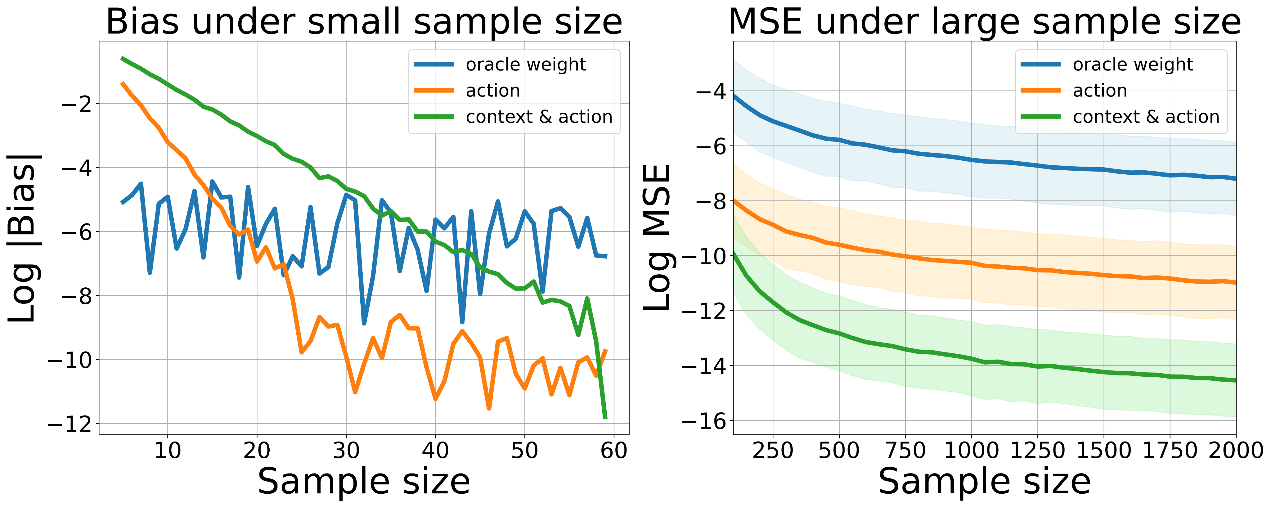
Our numerical results, reported in Figure 1, empirically confirm these conclusions. As observed in the right panel, incorporating context-dependent estimated IS ratios substantially reduces the MSE. Given that the -axis visualizes the log(MSE), even seemingly close log values can correspond to considerable differences in MSE values.
In what follows, we outline a sketch of the proof to demystify these results. The key insight is that replacing the true behavior policy with its estimator in the IS ratio plays a similar role in adding an augmentation term to the IS estimator. This modification effectively transforms the resulting estimator into a DR estimator, which is often more efficient than IS even in bandit settings (Tsiatis, 2006; Zhang et al., 2012; Dudík et al., 2014).
Specifically, it can be shown that and equal
respectively, where both and denote the sample mean estimators, obtained by averaging rewards across different contexts and/or actions.
In both expressions, the first terms within the curly brackets represent the direct method estimators for the policy value whereas the second terms serve as augmentation terms. The inclusion of these augmentation terms offers two advantages: (i) It debiases the bias inherent in the reward estimators, rendering the resulting OPE estimator asymptotically unbiased. (ii) It effectively reduces the variance of the OPE estimator by contrasting the observed reward with their predictor. Specifically, it can be shown that both expressions achieve no larger asymptotic variances than which uses the oracle IS ratio. Additionally, the variance reductions are likely substantial when the reward function differs significantly from . These discussions verify the assertions in Lemma 1.
In summary, our bandit example has revealed several intriguing conclusions that we aim to establish in MDPs. First, we will demonstrate that Conclusion 1 remains valid across a range of IS-type estimators with history-dependent behavior policy estimators in MDPs. Second, we will expand on Conclusion 2 by demonstrating that estimating a behavior policy that conditions on history leads to more accurate OPE estimators in large samples – even when the true behavior policy does not condition on more than the immediate preceding state. Finally, the above theoretical analysis did not consider the biases of IS estimators. As depicted in the left panel of Figure 1, incorporating history-dependent behavior policy estimation can increase bias in small samples. In our forthcoming analysis of MDPs, we will carefully examine the finite-sample biases of different IS estimators.
3.2 OPE in MDPs
Markov decision processes. This paper focuses on a finite-horizon MDP model characterized by a state space , an action space , a transition kernel , a reward function and a finite horizon . Consider a trajectory generated in . These data are generated as follows:
-
•
At each time, suppose the environment arrives at a given state ;
-
•
The agent then selects an action according to a behavior policy ;
-
•
Next, the environment provides an immediate reward to the agent whose expected value is specified by the reward function ;
-
•
Finally, the environment transits into a new state at time according to the transition function .
This process repeats until the termination time, , is reached.
Common IS-type estimators. Given an offline dataset with i.i.d. trajectories, the objective of OPE is to learn the expected cumulative reward under a different target policy , where denotes the discount factor and denotes the expectation assuming the actions are assigned according to .
Let denote the empirical average operator over the trajectories in the offline dataset and denote the product of IS ratios up to time . Below, we detail the definitions of the three types of IS estimators introduced in Section 2, along with the DR estimator which also employs IS ratios for OPE:
-
1.
OIS serves as the most foundational estimator. It applies a single weight to reweight the entire empirical return , leading to .
-
2.
SIS modifies OIS by applying a time-dependent ratio to reweight each reward , resulting in . This adjustment reduces the variance associated with the product of IS ratios since, at each time , only ratios up to that time are used.
-
3.
DR further employs an estimated Q-function to reduce the variance of SIS. Specifically, let denote the Q-function under the target policy, which measures the cumulative reward starting from a given state-action pair
Given a Q-function estimator for , DR is defined by
with the convention that . Since employs the oracle IS ratio and leverages the double-robustness property, it remains consistent regardless of whether the Q-function is correctly specified.
-
4.
MIS further reduces the variances of the aforementioned three estimators by replacing – which is known to suffer from the curse of horizon (Liu et al., 2018) – with an MIS ratio given by where and are the marginal distributions of induced by policies and , respectively. This leads to .
We will investigate the theoretical properties of these estimators in the next two sections.
4 Demystifying the paradox in MDPs
In this section, we conduct a rigorous theoretical analysis to evaluate the impact of replacing the oracle behavior policy with an estimated history-dependent behavior policy for OPE. Our analysis accommodates all four estimators discussed in Section 3.2.
Although is a Markov policy, historical observations can still be utilized to estimate it. In particular, we define the following estimator that uses -step state-action history ,
for some policy class that satisfies the following monotonicity assumption:
Assumption 1 (Monotonicity).
.
Most commonly used policy classes based on logistic regression models or neural networks satisfy Assumption 1. We discuss this assumption in greater detail in Appendix C.2 and impose the following assumptions.
Assumption 2 (Realizability).
There exists some such that .
Assumption 3 (Bounded rewards).
There exists some constant such that almost surely for any .
Assumption 4 (Coverage).
There exist some constants such that all policy functions are lower bounded by , and holds for all state-action pair .
Assumption 5 (Differentiability).
All policies are twice differentiable with respect to the parameter , and both its first and second derivatives are uniformly bounded.
Assumption 6 (Non-singularity).
The Fisher information matrix of , denoted by , is non-singular.
We make a few remarks. First, realizability assumes that the policy class is rich enough to cover . It is a common assumption in machine learning (Shalev-Shwartz & Ben-David, 2014). It will be relaxed in Section 5 by permitting a nonzero approximation error. Second, the bounded rewards and coverage conditions are frequently assumed in the RL and OPE literature (see e.g., Chen & Jiang, 2019; Fan et al., 2020; Kallus & Uehara, 2022). Finally, Assumptions 5 and 6 are widely imposed in statistics to establish the theoretical properties of maximum likelihood estimators (see e.g., Casella & Berger, 2024).
4.1 Ordinary IS estimator
Recall from Section 3.2 that denotes the OIS estimator with the oracle IS ratio . Let denote the version that uses the -step state-action history to compute the behavior policy estimator and plugs it into to construct the ratio estimator ,
The following theorem establishes the theoretical properties of these estimators.
Theorem 2.
Assume Assumptions 1 – 6 hold. Then
| (2) |
where denotes the space of mean zero random variables that is orthogonal to the tangent space spanned by the score vector
and denotes the projection of a given random variable onto the space of ; refer to Appendix C.2 for the detailed definitions. Moreover, for any , we have
| (3) | ||||
Theorem 2 has a number of important implications:
-
1.
Equation (2) obtains a bias-variance decomposition for the MSE of . In particular, the first term on the right-hand-side (RHS) of (2) corresponds to its asymptotic variance, which is of the order , whereas the second term upper bounds its finite-sample bias, which decays to zero at a faster rate as increases. Additionally, it is well known that the variances of IS-type estimators grow exponentially fast with the time horizon (see, e.g., Liu et al., 2018). Our error bound reveals that when using estimated IS ratios, the same curse of horizon applies to the bias, which includes a factor of for some , where if and only if the behavior policy matches the target policy, meaning there is no off-policy distributional shift at all.
-
2.
In large samples, the asymptotic variance term becomes the dominating factor. This term equals the variance of . Thus, incorporating history-dependent behavior policy estimation into OIS estimators can be interpreted as a projection that projects the empirical return into a more constrained space for variance reduction. This interpretation aligns with our perspective on transforming IS estimators with estimated ratios into DR estimators, as illustrated in the bandit example (see Section 3.1), since DR can be viewed as projecting an IS estimator onto a specific augmentation space to improve efficiency (Tsiatis, 2006). Notice that the projected variable achieves a smaller variance than itself, our result thus covers Corollary 2 in Hanna et al. (2021), suggesting that replacing the true behavior policy with its estimate reduces the asymptotic variance of the resulting OIS estimator.
-
3.
Additionally, according to (3), the variance term is a monotonically non-decreasing function with respect to the history-length, which in turn demonstrates the advantage of estimating a high-order Markov policy over a first-order policy in large samples. Mathematically, this can again be interpreted through projection: the longer the history-length, the more restrictive the constrained space used to project the empirical return, leading to greater asymptotic efficiency.
-
4.
In small samples, particularly in settings with long horizons, the bias term becomes non-negligible and increases exponentially with the horizon. To the contrary, the oracle estimator is unbiased. This illustrates the risk of employing history-dependent behavior policy estimation in small samples.
Based on the aforementioned discussion, the following corollary is immediate from Theorem 2.
To summarize, Theorem 2 formally establishes the bias-variance trade-off in history-dependent behavior policy estimation: it decreases the asymptotic variance of the OIS estimator at the cost of increasing the finite-sample bias. Furthermore, a longer history length results in a greater reduction in variance.
4.2 Sequential IS estimator
Let denote the estimator for by replacing the oracle behavior policy with its estimator . We define as a variant of the oracle SIS estimator constructed based on . The following theorem obtains a similar bias-variance decomposition for its MSE.
Theorem 4.
Recall that the oracle SIS estimator is given by . Similar to OIS, Theorem 4 suggests that using an estimated behavior policy will lower the MSE of the resulting SIS estimator in large samples through projection. Meanwhile, the longer the history-length, the lower the asymptotic MSE, leading to the following corollary.
However, estimating the behavior policy can introduce significant biases in small samples and long horizons, the magnitudes of which are given by the second term in (4).
4.3 Doubly robust estimator
Consider the following DR estimator constructed based on the history-dependent IS ratio ,
with a pre-specified Q-function which is required to satisfy the following assumption:
Assumption 7 (Boundedness).
There exists some such that the absolute value of is upper bounded by almost surely for any .
Assumption 7 corresponds to a version of the boundedness condition in Assumption 3 tailored for DR estimators. The constant is expected to be much smaller than with a well-chosen Q-function. In particular, when the Q-function is correctly specified, corresponds to the absolute value of the Bellman residual, which tends to concentrate more closely around zero than .
Theorem 6.
We make two remarks regarding Theorem 6:
-
1.
The bias-variance decomposition in (5) closely resembles that of SIS, with the key difference being that the reward and its bound in (4) are replaced with and , respectively. With a well-specified Q-function, is expected to exhibit lower variability than , and can be significantly smaller than . This highlights the advantages of history-dependent DR estimators over SIS: they not only improve asymptotic variance but also reduce finite-sample bias.
-
2.
However, the second part of Theorem 6 indicates that, unlike OIS or SIS, history-dependent behavior policy estimation may not further reduce asymptotic variance when the Q-function is correctly specified. This is intuitive, as in such cases, the DR estimator is known to achieve certain efficiency bounds (Jiang & Li, 2016; Kallus & Uehara, 2020). If the estimator is already efficient, history-dependent behavior policy estimation cannot provide additional gains. On the other hand, when the Q-function is misspecified, there remains room for improvement, and history-dependent estimators can improve the estimation accuracy.
The following corollary is again an immediate application of Theorem 5.
4.4 Marginalized importance sampling estimator
A key step in constructing the MIS estimator lies in the estimation of the MIS ratio. Unlike the previously discussed ratios , which can be known in settings such as randomized studies, the MIS ratio depends on the marginal state distribution and is typically unknown, even when the behavior policy is given.
In the literature, several methods have been developed to estimate the MIS ratio, such as minimax learning (Uehara et al., 2020) and reproducing kernel Hilbert space (RKHS)-based methods (Liao et al., 2022). To simplify the analysis, we focus on using linear function approximation in this paper, which parameterizes each by , for some state-action features . Adapting Example 2 from Uehara et al. (2020) to the finite-horizon setting, we derive the following closed-form expression for the estimator ,
where , and the following recursive formulas for computing ,
The estimated MIS ratios are then plugged into the oracle estimator to compute .
Alternatively, the -step history can be used to construct a history-dependent MIS ratio . This ratio can be interpreted as a conditional IS ratio (Rowland et al., 2020) with and being the conditioning variable. It is also closely related to the incremental IS (INCRIS) ratio proposed by Guo et al. (2017), but differs by incorporating an additional MIS ratio for .
For estimation, can be parameterized similarly to , using -step features as a function of and , with parameters estimated in a manner similar to those for . However, unlike IS and DR, incorporating a history-dependent MIS ratio may increase the MSE of the resulting MIS estimator, denoted by . Additionally, the longer the history-length, the worsen the performance. We summarize these results in the following theorem.
Theorem 8.
Let be the MIS estimator with -step history: Then, under regularity conditions specified in Appendix C.2, for any ,
To appreciate why Theorem 8 holds, notice that by setting to the horizon , is reduced to the , and the resulting estimator is reduced to SIS, which suffers from the curse of horizon and is known to be less efficient than MIS. More generally, similar to , increasing the history-length leads to a more variable IS ratio, thus increasing the MSE.
5 Extensions to cases where the behavior policy is estimated nonparametrically
Our analysis so far focuses on using parametric models to estimate the behavior policy or IS ratio. In practical applications, nonparametric estimation of the behavior policy can be desirable to avoid the potential misspecification of the parametric model. This motivates us to investigate the performance of history-dependent OPE estimators with nonparametrically estimated behavior policy.
A common nonparametric approach is to approximate the policy set using a sequence of sieve spaces . Below, we demonstrate that, under certain regularity conditions (detailed in Appendix C.3), similar to the parametric case, replacing the true behavior policy with an estimated behavior policy within the sieve space lowers the asymptotic variance of the resulting OPE estimator.
Specifically, we assume the policy class can be represented by with an infinite-dimensional Hilbert space . Let be a sequence of finite-dimensional sieve spaces. For a given sample size , we compute the estimator by maximizing the log-likelihood function in the sieve space ,
Let , and denote the OIS, SIS and DR estimators, respectively, each constructed based on the estimated behavior policy . We summarize our results as follows.
Theorem 9 demonstrates the advantages of OPE estimators with nonparametrically estimated behavior policies in large samples. While similar results have been established in the literature (see e.g., Hanna et al., 2021), they primarily focused on the OIS estimator using parametric estimation of the behavior policy and required the realizability assumption (see Assumption 2). In contrast, Theorem 9 relaxes the realizability by allowing the approximation error to decay to zero at a rate of (see Assumption 9), which is much slower than the parametric -rate. Nonetheless, we demonstrate that the resulting OPE estimators still converge at the parametric rate, which is central to establish their MSEs. This faster convergence rate occurs because the policy value is a smooth functional of the sieve estimator, and “smoothing” inherently improves the convergence rate. While similar findings have been documented in classical statistics literature for nonparametric regression problems (Shen, 1997; Newey et al., 1998), these phenomena have not been less explored in OPE and RL. One exception is Shi et al. (2023), who considered the direct method estimator but did not study history-dependent behavior policy estimation.
6 Numerical studies
Our experiment compares several history-dependent IS estimators in the CartPole environment (Brockman et al., 2016). Specifically, we consider the following three estimators: SIS, DR with a misspecified Q-function, and MIS.
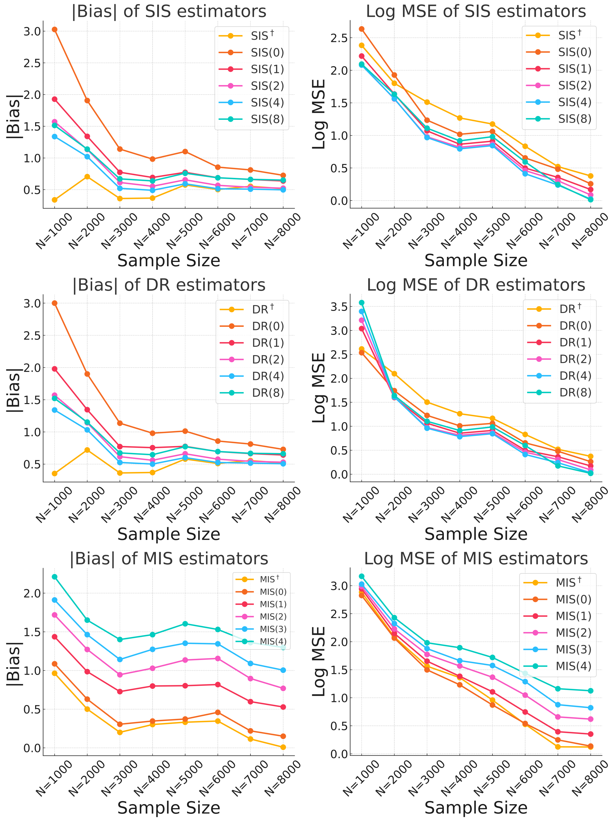
As shown in Figure 2, all three estimators’ MSEs decrease with the sample size, suggesting their consistencies. For SIS and DR with misspecified Q-functions, replacing the oracle behavior policy with a history-dependent estimator generally reduces their MSEs in large samples. Additionally, performance improves with longer history-length. However, for MIS estimators, the performance consistently worsens as we increase the history-length to estimate the MIS ratio. Finally, it is also apparent that history-dependent estimators generally suffer from larger biases compared to those using an oracle behavior policy. These empirical results verify our theoretical findings.
In Appendix B, we further expand our numerical experiments to more complex MuJoCo environments, including (i) Inverted Pendulum, featuring a continuous action space; (ii) Double Inverted Pendulum, characterized by a higher-dimensional state space; (iii) Swimmer, an environment with substantially different dynamics compared to the other two. The detailed results are deferred to Appendix B.
7 Discussion
This paper demystifies the paradox concerning the impact of history-dependent behavior policy estimation on IS-type OPE estimators by establishing a bias-variance decomposition of their MSEs. Our analysis reveals a trade-off in the choice of history-length for estimating the behavior policy: increasing the history-length reduces the estimator’s asymptotic variance, but can increase its finite-sample bias. Therefore, selection of history length is crucial for applying our theory to practice.
In this section, we propose some practical guidance on the selection of history length when estimating behavior policy. Specifically, motivated by the bias-variance trade-off, we propose to select the history length that minimizes
where denotes variance estimator computed via the sampling variance formula or bootstrap, is the Bayesian information criterion (BIC, Schwarz, 1978) penalty preventing selecting long history without substantial reduction of the variance. Our simulation studies (not reported in the paper) demonstrate strong empirical performance of this history selection method.
To conclude this paper, we note that the OPE literature has been growing rapidly in recent years, expanding into several directions, including the investigation of partially observable environments (Uehara et al., 2023; Hu & Wager, 2023), heavy-tailed rewards (Xu et al., 2022; Liu et al., 2023; Rowland et al., 2023; Zhu et al., 2024; Behnamnia et al., 2025) and unmeasured confounders (Kallus & Zhou, 2020; Namkoong et al., 2020; Tennenholtz et al., 2020; Nair & Jiang, 2021; Shi et al., 2022a; Wang et al., 2022; Bruns-Smith & Zhou, 2023; Xu et al., 2023; Bennett & Kallus, 2024; Shi et al., 2024; Yu et al., 2024). Our proposal is related to a growing line of research that investigates optimal experimental design for OPE (Hanna et al., 2017; Mukherjee et al., 2022; Wan et al., 2022; Li et al., 2023; Liu & Zhang, 2024; Liu et al., 2024; Sun et al., 2024; Wen et al., 2025). These works focus on designing optimal behavior policies prior to data collection to improve OPE accuracy whereas our proposal considers estimating behavior policies after data collection for the same purpose. The work of Liu & Zhang (2024) is particularly related as the behavior policy is computed from offline data before being run to collect more data. Both approaches share the most fundamental goal of enhancing OPE by learning behavior policies - whether for data collection or retrospective estimation.
Acknowledgement
Hongyi Zhou’s and Ying Yang’s research was partially supported by NSFC 12271286 & 11931001. Hongyi Zhou’s research was also partially supported by the China Scholarship Council. Chengchun Shi’s and Jin Zhu’s research was partially supported by the EPSRC grant EP/W014971/1. Josiah Hanna acknowledges support from NSF (IIS-2410981), American Family Insurance through a research partnership with the University of Wisconsin—Madison’s Data Science Institute, the Wisconsin Alumni Research Foundation, and Sandia National Labs through a University Partnership Award. The authors thank the anonymous referees and the area chair for their insightful and constructive comments, which have led to a significantly improved version of the paper.
Impact statement
This paper provides a theoretical foundation for using history-dependent behavior policy estimators for OPE in reinforcement learning. Our research reveals that while these estimators may decrease accuracy with small sample sizes, they significantly improve estimation accuracy as sample size increases. This insight clarifies when and how historical data should be integrated into behavior policy estimation, enhancing the effectiveness and reliability of various off-policy estimators across different applications. Our work primarily engages in theoretical analysis and does not directly interact with or manipulate real-world systems. Consequently, it is unlikely to have negative societal consequences.
References
- Behnamnia et al. (2025) Behnamnia, A., Aminian, G., Aghaei, A., Shi, C., Tan, V. Y. F., and Rabiee, H. R. Log-sum-exponential estimator for off-policy evaluation and learning. In International Conference on Machine Learning. PMLR, 2025.
- Bennett & Kallus (2024) Bennett, A. and Kallus, N. Proximal reinforcement learning: Efficient off-policy evaluation in partially observed markov decision processes. Operations Research, 72(3):1071–1086, 2024.
- Bian et al. (2025) Bian, Z., Shi, C., Qi, Z., and Wang, L. Off-policy evaluation in doubly inhomogeneous environments. Journal of the American Statistical Association, to appear, 2025.
- Bibaut et al. (2019) Bibaut, A., Malenica, I., Vlassis, N., and Van Der Laan, M. More efficient off-policy evaluation through regularized targeted learning. In International Conference on Machine Learning, pp. 654–663. PMLR, 2019.
- Bossens & Thomas (2024) Bossens, D. M. and Thomas, P. S. Low variance off-policy evaluation with state-based importance sampling. In 2024 IEEE Conference on Artificial Intelligence (CAI), pp. 871–883. IEEE, 2024.
- Brockman et al. (2016) Brockman, G., Cheung, V., Pettersson, L., Schneider, J., Schulman, J., Tang, J., and Zaremba, W. Openai gym, 2016. URL https://arxiv.org/abs/1606.01540.
- Bruns-Smith & Zhou (2023) Bruns-Smith, D. and Zhou, A. Robust fitted-q-evaluation and iteration under sequentially exogenous unobserved confounders. arXiv preprint arXiv:2302.00662, 2023.
- Cao & Zhou (2024) Cao, D. and Zhou, A. Orthogonalized estimation of difference of -functions. arXiv preprint arXiv:2406.08697, 2024.
- Casella & Berger (2024) Casella, G. and Berger, R. Statistical inference. CRC press, 2024.
- Chapelle & Li (2011) Chapelle, O. and Li, L. An empirical evaluation of thompson sampling. In Proceedings of the 24th International Conference on Neural Information Processing Systems, NIPS’11, pp. 2249–2257, Red Hook, NY, USA, 2011. Curran Associates Inc. ISBN 9781618395993.
- Chen & Jiang (2019) Chen, J. and Jiang, N. Information-theoretic considerations in batch reinforcement learning. In International Conference on Machine Learning, pp. 1042–1051. PMLR, 2019.
- Chen & Qi (2022) Chen, X. and Qi, Z. On well-posedness and minimax optimal rates of nonparametric q-function estimation in off-policy evaluation. In Proceedings of the 39th International Conference on Machine Learning, volume 162 of Proceedings of Machine Learning Research, pp. 3558–3582. PMLR, 17–23 Jul 2022.
- Chernozhukov et al. (2014) Chernozhukov, V., Chetverikov, D., and Kato, K. Gaussian approximation of suprema of empirical processes. The Annals of Statistics, pp. 1564–1597, 2014.
- Chernozhukov et al. (2018) Chernozhukov, V., Chetverikov, D., Demirer, M., Duflo, E., Hansen, C., Newey, W., and Robins, J. Double/debiased machine learning for treatment and structural parameters. The Econometrics Journal, 21(1):C1–C68, 01 2018.
- Dai et al. (2020) Dai, B., Nachum, O., Chow, Y., Li, L., Szepesvari, C., and Schuurmans, D. Coindice: Off-policy confidence interval estimation. In Advances in Neural Information Processing Systems, volume 33, pp. 9398–9411. Curran Associates, Inc., 2020.
- Dudík et al. (2014) Dudík, M., Erhan, D., Langford, J., and Li, L. Doubly Robust Policy Evaluation and Optimization. Statistical Science, 29(4):485 – 511, 2014. doi: 10.1214/14-STS500.
- Fan et al. (2020) Fan, J., Wang, Z., Xie, Y., and Yang, Z. A theoretical analysis of deep q-learning. In Learning for dynamics and control, pp. 486–489. PMLR, 2020.
- Farajtabar et al. (2018) Farajtabar, M., Chow, Y., and Ghavamzadeh, M. More robust doubly robust off-policy evaluation. ArXiv, abs/1802.03493, 2018.
- Feng et al. (2020) Feng, Y., Ren, T., Tang, Z., and Liu, Q. Accountable off-policy evaluation with kernel Bellman statistics. In Proceedings of the 37th International Conference on Machine Learning, volume 119 of Proceedings of Machine Learning Research, pp. 3102–3111. PMLR, 13–18 Jul 2020.
- Gottesman et al. (2019) Gottesman, O., Liu, Y., Sussex, S., Brunskill, E., and Doshi-Velez, F. Combining parametric and nonparametric models for off-policy evaluation. In International Conference on Machine Learning, pp. 2366–2375. PMLR, 2019.
- Guo et al. (2017) Guo, Z. D., Thomas, P. S., and Brunskill, E. Using options and covariance testing for long horizon off-policy policy evaluation. In Proceedings of the 31st International Conference on Neural Information Processing Systems, NIPS’17, pp. 2489–2498, Red Hook, NY, USA, 2017. Curran Associates Inc. ISBN 9781510860964.
- Hanna et al. (2019) Hanna, J., Niekum, S., and Stone, P. Importance sampling policy evaluation with an estimated behavior policy. In Proceedings of the 36th International Conference on Machine Learning, volume 97 of Proceedings of Machine Learning Research, pp. 2605–2613. PMLR, 09–15 Jun 2019.
- Hanna et al. (2017) Hanna, J. P., Thomas, P. S., Stone, P., and Niekum, S. Data-efficient policy evaluation through behavior policy search. In Precup, D. and Teh, Y. W. (eds.), Proceedings of the 34th International Conference on Machine Learning, volume 70 of Proceedings of Machine Learning Research, pp. 1394–1403. PMLR, 06–11 Aug 2017.
- Hanna et al. (2021) Hanna, J. P., Niekum, S., and Stone, P. Importance sampling in reinforcement learning with an estimated behavior policy. Mach. Learn., 110(6):1267–1317, 2021. ISSN 0885-6125.
- Hao et al. (2021) Hao, B., Ji, X., Duan, Y., Lu, H., Szepesvari, C., and Wang, M. Bootstrapping fitted q-evaluation for off-policy inference. In Proceedings of the 38th International Conference on Machine Learning, volume 139 of Proceedings of Machine Learning Research, pp. 4074–4084. PMLR, 2021.
- Henmi et al. (2007) Henmi, M., Yoshida, R., and Eguchi, S. Importance sampling via the estimated sampler. Biometrika, 94(4):985–991, 12 2007.
- Hirano et al. (2003) Hirano, K., Imbens, G. W., and Ridder, G. Efficient estimation of average treatment effects using the estimated propensity score. Econometrica, 71(4):1161–1189, 2003.
- Hu & Wager (2023) Hu, Y. and Wager, S. Off-policy evaluation in partially observed Markov decision processes under sequential ignorability. The Annals of Statistics, 51(4):1561 – 1585, 2023. doi: 10.1214/23-AOS2287.
- Jiang & Li (2016) Jiang, N. and Li, L. Doubly robust off-policy value evaluation for reinforcement learning. In Proceedings of The 33rd International Conference on Machine Learning, volume 48 of Proceedings of Machine Learning Research, pp. 652–661, New York, New York, USA, 20–22 Jun 2016. PMLR.
- Kallus & Uehara (2020) Kallus, N. and Uehara, M. Double reinforcement learning for efficient off-policy evaluation in markov decision processes. Journal of Machine Learning Research, 21(167):1–63, 2020. URL http://jmlr.org/papers/v21/19-827.html.
- Kallus & Uehara (2022) Kallus, N. and Uehara, M. Efficiently breaking the curse of horizon in off-policy evaluation with double reinforcement learning. Oper. Res., 70(6):3282–3302, November 2022. ISSN 0030-364X.
- Kallus & Zhou (2020) Kallus, N. and Zhou, A. Confounding-robust policy evaluation in infinite-horizon reinforcement learning. Advances in neural information processing systems, 33:22293–22304, 2020.
- Kosorok (2008) Kosorok, M. R. Introduction to Empirical Processes and Semiparametric Inference. Springer New York, NY, 2008.
- Le et al. (2019) Le, H., Voloshin, C., and Yue, Y. Batch policy learning under constraints. In Proceedings of the 36th International Conference on Machine Learning, volume 97 of Proceedings of Machine Learning Research, pp. 3703–3712. PMLR, 09–15 Jun 2019.
- Levine et al. (2020) Levine, S., Kumar, A., Tucker, G., and Fu, J. Offline reinforcement learning: Tutorial, review, and perspectives on open problems. ArXiv, abs/2005.01643, 2020.
- Li et al. (2023) Li, G., Wu, W., Chi, Y., Ma, C., Rinaldo, A., and Wei, Y. Sharp high-probability sample complexities for policy evaluation with linear function approximation. arXiv preprint arXiv:2305.19001, 2023.
- Liao et al. (2021) Liao, P., Klasnja, P., and Murphy, S. Off-policy estimation of long-term average outcomes with applications to mobile health. Journal of the American Statistical Association, 116(533):382–391, 2021.
- Liao et al. (2022) Liao, P., Qi, Z., Wan, R., Klasnja, P., and Murphy, S. A. Batch policy learning in average reward Markov decision processes. The Annals of Statistics, 50(6):3364 – 3387, 2022.
- Liu et al. (2018) Liu, Q., Li, L., Tang, Z., and Zhou, D. Breaking the curse of horizon: infinite-horizon off-policy estimation. In Proceedings of the 32nd International Conference on Neural Information Processing Systems, NIPS’18, pp. 5361–5371, Red Hook, NY, USA, 2018. Curran Associates Inc.
- Liu & Zhang (2024) Liu, S. and Zhang, S. Efficient policy evaluation with offline data informed behavior policy design. In Salakhutdinov, R., Kolter, Z., Heller, K., Weller, A., Oliver, N., Scarlett, J., and Berkenkamp, F. (eds.), Proceedings of the 41st International Conference on Machine Learning, volume 235 of Proceedings of Machine Learning Research, pp. 32345–32368. PMLR, 21–27 Jul 2024.
- Liu et al. (2024) Liu, S. D., Chen, C., and Zhang, S. Doubly optimal policy evaluation for reinforcement learning. arXiv preprint arXiv:2410.02226, 2024.
- Liu et al. (2023) Liu, W., Tu, J., Zhang, Y., and Chen, X. Online estimation and inference for robust policy evaluation in reinforcement learning. arXiv preprint arXiv:2310.02581, 2023.
- Luckett et al. (2020) Luckett, D. J., Laber, E. B., Kahkoska, A. R., David M. Maahs, E. M.-D., and Kosorok, M. R. Estimating dynamic treatment regimes in mobile health using v-learning. Journal of the American Statistical Association, 115(530):692–706, 2020. doi: 10.1080/01621459.2018.1537919.
- Mukherjee et al. (2022) Mukherjee, S., Hanna, J. P., and Nowak, R. D. Revar: Strengthening policy evaluation via reduced variance sampling. In Cussens, J. and Zhang, K. (eds.), Proceedings of the Thirty-Eighth Conference on Uncertainty in Artificial Intelligence, volume 180 of Proceedings of Machine Learning Research, pp. 1413–1422. PMLR, 01–05 Aug 2022.
- Murphy et al. (2001) Murphy, S. A., van der Laan, M. J., Robins, J. M., and Group, C. P. P. R. Marginal mean models for dynamic regimes. Journal of the American Statistical Association, 96(456):1410–1423, 2001.
- Nachum et al. (2019) Nachum, O., Chow, Y., Dai, B., and Li, L. Dualdice: Behavior-agnostic estimation of discounted stationary distribution corrections. Advances in neural information processing systems, 32, 2019.
- Nair & Jiang (2021) Nair, Y. and Jiang, N. A spectral approach to off-policy evaluation for pomdps. arXiv preprint arXiv:2109.10502, 2021.
- Namkoong et al. (2020) Namkoong, H., Keramati, R., Yadlowsky, S., and Brunskill, E. Off-policy policy evaluation for sequential decisions under unobserved confounding. Advances in Neural Information Processing Systems, 33:18819–18831, 2020.
- Newey et al. (1998) Newey, W. K., Hsieh, F., and Robins, J. Undersmoothing and bias corrected functional estimation. 1998.
- Ouyang et al. (2022) Ouyang, L., Wu, J., Jiang, X., Almeida, D., Wainwright, C., Mishkin, P., Zhang, C., Agarwal, S., Slama, K., Ray, A., et al. Training language models to follow instructions with human feedback. Advances in neural information processing systems, 35:27730–27744, 2022.
- Precup et al. (2000) Precup, D., Sutton, R. S., and Singh, S. P. Eligibility traces for off-policy policy evaluation. In Proceedings of the Seventeenth International Conference on Machine Learning, ICML ’00, pp. 759–766, San Francisco, CA, USA, 2000. Morgan Kaufmann Publishers Inc. ISBN 1558607072.
- Puterman (2014) Puterman, M. L. Markov decision processes: discrete stochastic dynamic programming. John Wiley & Sons, 2014.
- Rosenbaum & Rubin (1983) Rosenbaum, P. R. and Rubin, D. B. The central role of the propensity score in observational studies for causal effects. Biometrika, 70(1):41–55, 1983. ISSN 00063444, 14643510.
- Rowland et al. (2020) Rowland, M., Harutyunyan, A., Hasselt, H., Borsa, D., Schaul, T., Munos, R., and Dabney, W. Conditional importance sampling for off-policy learning. In International Conference on Artificial Intelligence and Statistics, pp. 45–55. PMLR, 2020.
- Rowland et al. (2023) Rowland, M., Tang, Y., Lyle, C., Munos, R., Bellemare, M. G., and Dabney, W. The statistical benefits of quantile temporal-difference learning for value estimation. In International Conference on Machine Learning, pp. 29210–29231. PMLR, 2023.
- Schulman et al. (2017) Schulman, J., Wolski, F., Dhariwal, P., Radford, A., and Klimov, O. Proximal policy optimization algorithms. arXiv preprint arXiv:1707.06347, 2017.
- Schwarz (1978) Schwarz, G. Estimating the dimension of a model. The annals of statistics, pp. 461–464, 1978.
- Shalev-Shwartz & Ben-David (2014) Shalev-Shwartz, S. and Ben-David, S. Understanding machine learning: From theory to algorithms. Cambridge university press, 2014.
- Shao (2003) Shao, J. Mathematical Statistics. Springer, New York, 2nd edition, 2003. ISBN 978-0-387-00179-1. doi: 10.1007/b98854.
- Shen (1997) Shen, X. On methods of sieves and penalization. The Annals of Statistics, 25(6):2555–2591, 1997.
- Shi et al. (2021) Shi, C., Wan, R., Chernozhukov, V., and Song, R. Deeply-debiased off-policy interval estimation. In International conference on machine learning, pp. 9580–9591. PMLR, 2021.
- Shi et al. (2022a) Shi, C., Uehara, M., Huang, J., and Jiang, N. A minimax learning approach to off-policy evaluation in confounded partially observable markov decision processes. In International Conference on Machine Learning, pp. 20057–20094. PMLR, 2022a.
- Shi et al. (2022b) Shi, C., Zhang, S., Lu, W., and Song, R. Statistical inference of the value function for reinforcement learning in infinite-horizon settings. Journal of the Royal Statistical Society Series B: Statistical Methodology, 84(3):765–793, 12 2022b.
- Shi et al. (2023) Shi, C., Wang, X., Luo, S., Zhu, H., Ye, J., and Song, R. Dynamic causal effects evaluation in a/b testing with a reinforcement learning framework. Journal of the American Statistical Association, 118(543):2059–2071, 2023.
- Shi et al. (2024) Shi, C., Zhu, J., Shen, Y., Luo, S., Zhu, H., and Song, R. Off-policy confidence interval estimation with confounded markov decision process. Journal of the American Statistical Association, 119(545):273–284, 2024.
- Sun et al. (2024) Sun, K., Kong, L., Zhu, H., and Shi, C. Optimal treatment allocation strategies for a/b testing in partially observable time series experiments. arXiv preprint arXiv:2408.05342, 2024.
- Sutton et al. (2008) Sutton, R. S., Szepesvári, C., and Maei, H. R. A convergent o(n) algorithm for off-policy temporal-difference learning with linear function approximation. Advances in neural information processing systems, 21(21):1609–1616, 2008.
- Tang et al. (2020) Tang, Z., Feng, Y., Li, L., Zhou, D., and Liu, Q. Doubly robust bias reduction in infinite horizon off-policy estimation. In International Conference on Learning Representations, 2020.
- Tennenholtz et al. (2020) Tennenholtz, G., Shalit, U., and Mannor, S. Off-policy evaluation in partially observable environments. In Proceedings of the AAAI Conference on Artificial Intelligence, volume 34, pp. 10276–10283, 2020.
- Thomas & Brunskill (2016) Thomas, P. S. and Brunskill, E. Data-efficient off-policy policy evaluation for reinforcement learning. In Proceedings of the 33rd International Conference on International Conference on Machine Learning - Volume 48, ICML’16, pp. 2139–2148. JMLR.org, 2016.
- Thomas et al. (2015) Thomas, P. S., Theocharous, G., and Ghavamzadeh, M. High-confidence off-policy evaluation. In AAAI Conference on Artificial Intelligence, 2015.
- Tsiatis (2006) Tsiatis, A. A. Semiparametric Theory and Missing Data. Springer, 2006.
- Uehara et al. (2020) Uehara, M., Huang, J., and Jiang, N. Minimax weight and q-function learning for off-policy evaluation. In Proceedings of the 37th International Conference on Machine Learning, volume 119 of Proceedings of Machine Learning Research, pp. 9659–9668. PMLR, 13–18 Jul 2020.
- Uehara et al. (2022) Uehara, M., Shi, C., and Kallus, N. A review of off-policy evaluation in reinforcement learning. arXiv preprint arXiv:2212.06355, 2022.
- Uehara et al. (2023) Uehara, M., Kiyohara, H., Bennett, A., Chernozhukov, V., Jiang, N., Kallus, N., Shi, C., and Sun, W. Future-dependent value-based off-policy evaluation in pomdps. In Advances in Neural Information Processing Systems, volume 36, pp. 15991–16008. Curran Associates, Inc., 2023.
- Van Der Vaart et al. (1996) Van Der Vaart, A. W., Wellner, J. A., van der Vaart, A. W., and Wellner, J. A. Weak convergence. Springer, 1996.
- Wan et al. (2022) Wan, R., Kveton, B., and Song, R. Safe exploration for efficient policy evaluation and comparison. In International Conference on Machine Learning, pp. 22491–22511. PMLR, 2022.
- Wang et al. (2022) Wang, J., Qi, Z., and Shi, C. Blessing from human-ai interaction: Super reinforcement learning in confounded environments. arXiv preprint arXiv:2209.15448, 2022.
- Wang et al. (2023) Wang, J., Qi, Z., and Wong, R. K. W. Projected state-action balancing weights for offline reinforcement learning. The Annals of Statistics, 51(4):1639 – 1665, 2023.
- Wang et al. (2024) Wang, W., Li, Y., and Wu, X. Off-policy evaluation for tabular reinforcement learning with synthetic trajectories. Statistics and Computing, 34(1):41, 2024.
- Wen et al. (2025) Wen, Q., Shi, C., Yang, Y., Tang, N., and Zhu, H. Unraveling the interplay between carryover effects and reward autocorrelations in switchback experiments. In International Conference on Machine Learning. PMLR, 2025.
- Xie et al. (2023) Xie, C., Yang, W., and Zhang, Z. Semiparametrically efficient off-policy evaluation in linear markov decision processes. In International Conference on Machine Learning, pp. 38227–38257. PMLR, 2023.
- Xie et al. (2019a) Xie, T., Ma, Y., and Wang, Y.-X. Towards optimal off-policy evaluation for reinforcement learning with marginalized importance sampling. Curran Associates Inc., Red Hook, NY, USA, 2019a.
- Xie et al. (2019b) Xie, T., Ma, Y., and Wang, Y.-X. Towards optimal off-policy evaluation for reinforcement learning with marginalized importance sampling. Advances in neural information processing systems, 32, 2019b.
- Xu et al. (2022) Xu, Y., Shi, C., Luo, S., Wang, L., and Song, R. Quantile off-policy evaluation via deep conditional generative learning. arXiv preprint arXiv:2212.14466, 2022.
- Xu et al. (2023) Xu, Y., Zhu, J., Shi, C., Luo, S., and Song, R. An instrumental variable approach to confounded off-policy evaluation. In International Conference on Machine Learning, pp. 38848–38880. PMLR, 2023.
- Yin & Wang (2020) Yin, M. and Wang, Y.-X. Asymptotically efficient off-policy evaluation for tabular reinforcement learning. In International Conference on Artificial Intelligence and Statistics, pp. 3948–3958. PMLR, 2020.
- Yu et al. (2024) Yu, S., Fang, S., Peng, R., Qi, Z., Zhou, F., and Shi, C. Two-way deconfounder for off-policy evaluation in causal reinforcement learning. Advances in Neural Information Processing Systems, 37:78169–78200, 2024.
- Zhang et al. (2012) Zhang, B., Tsiatis, A. A., Laber, E. B., and Davidian, M. A robust method for estimating optimal treatment regimes. Biometrics, 68(4):1010–1018, 05 2012. ISSN 0006-341X.
- Zhang et al. (2013) Zhang, B., Tsiatis, A. A., Laber, E. B., and Davidian, M. Robust estimation of optimal dynamic treatment regimes for sequential treatment decisions. Biometrika, 100(3):681–694, 2013.
- Zhao & Zhang (2017) Zhao, X. and Zhang, Y. Asymptotic normality of nonparametric m-estimators with applications to hypothesis testing for panel count data. Statistica Sinica, 27:931–950, 2017. URL https://api.semanticscholar.org/CorpusID:54836455.
- Zhao et al. (2015) Zhao, Y.-Q., Zeng, D., Laber, E. B., and Kosorok, M. R. New statistical learning methods for estimating optimal dynamic treatment regimes. Journal of the American Statistical Association, 110(510):583–598, 2015.
- Zhou et al. (2023) Zhou, W., Li, Y., Zhu, R., and Qu, A. Distributional shift-aware off-policy interval estimation: A unified error quantification framework. arXiv preprint arXiv:2309.13278, 2023.
- Zhu et al. (2024) Zhu, J., Wan, R., Qi, Z., Luo, S., and Shi, C. Robust offline reinforcement learning with heavy-tailed rewards. In International Conference on Artificial Intelligence and Statistics, pp. 541–549. PMLR, 2024.
Appendix A Details of experiments
Bandit example in Section 3.1. In our illustrative example, we set the context space , the action space . The target policy is set as
The behavior policy is set as
Both the target and behavior policies are independent of context information. The context information follows a Bernoulli distribution with parameter , that is,
Given context information and action , the reward is a random variable with mean . Therefore, the reward function is a deterministic function defined as
For the illustrative example, we can derive the closed-form expression of the policy’s value, which is 4.2.
Numerical experiments in Section 6. In Cartpole environment, the state space is a subset of . For any , is characterized by four elements , where are the position and velocity of the cart, are the angle and angle velocity of the pole with the vertical axis. The behavior policy and the target policy are set as
Given , the reward is defined as . The maximum episode length is set as 200. We use a logistic regression model to estimate the behavior policy. The state transition model is set as the physical system implemented in CartPole environment in the gym library. And the initial state are uniformly drawn from .
We use a Monte Carlo (MC) procedure to approximate the true value of target policy. Specifically, we run the deploy the target policy to the simulator and get a empirical cumulative reward . The procedure is repeated times, and the MC estimator is given by
In our experiments, we set and the value of is 92.91.
Appendix B Additional experiment results
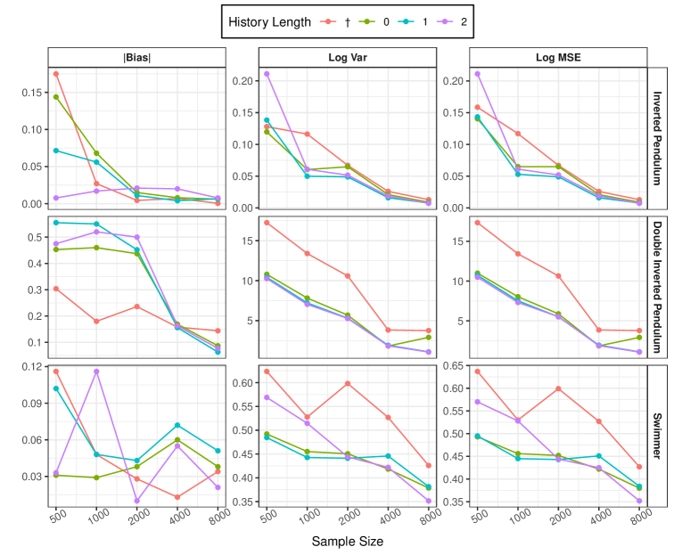
In this section, we examine the impact of using history-dependent behavior policies in the OIS estimator across three MuJoCo environments: (i) Inverted Pendulum; (ii) Double Inverted Pendulum and (iii) Swimmer.
For both Inverted Pendulum and Double Inverted Pendulum, the behavior policy is modeled using a transformed Beta distribution. Specifically, we set the action to , where and . The parameter is estimated by maximizing the log-likelihood.
In Swimmer, the action is two-dimensional, i.e., , and we sample each component independently given the state: and , with and .
The results, summarized in Figure 3, demonstrate that using history-dependent behavior policy estimation generally reduces the MSE of OIS in large-sample settings. Moreover, the performance tends to improve with longer history lengths.
We further evaluate the use of history-dependent behavior policies in the SIS, DR, and MIS estimators within the more complex Swimmer environment. Results, presented in Figure 4, again aligns with our theory.

Appendix C Proofs
C.1 Proof of Lemma 1
According to the definitions of and , it follows from straightforward calculations that
and
According to Neyman orthogonality, both the estimated reward and estimated behavior policy can be asymptotically replaced by its oracle value without changing the OPE estimator’s asymptotic MSE (Chernozhukov et al., 2018). As this part of the proof follows standard arguments, we provide only a sketch; interested readers may refer to, for example, the proof of Theorem 9 in Kallus & Uehara (2020) for further details.
Specifically, can be decomposed into the following four terms:
| (6) | |||||
| (7) | |||||
| (8) | |||||
| (9) |
Here, the right-hand-side (RHS) of (6) is the oracle DR estimator with the true reward function and IS ratio, and (7) – (9) are the reminder terms, which we will show are of order . In particular:
-
•
For fixed and , (7) and (8) are of zero mean. They are of the order provided that and converge to their oracle values. Even when and are estimated from the same data used in the evaluation, our use of tabular methods—combined with the fact that the number of contexts and actions is finite—ensures that these estimators belong to function classes with finite VC-dimension (Van Der Vaart et al., 1996). Therefore, standard empirical process theory (e.g., Chernozhukov et al., 2014, Corollary 5.1) can be applied to establish that these terms are indeed .
-
•
For fixed and , (9) is of the order where and denote the root MSEs (RMSEs) between and , and between and , respectively. Crucially, the order is the product of the two RMSEs. Consequently, as they decay to zero at a rate of – which is much slower than the parametric rate – this term becomes as well. Again, under tabular estimation with finitely many contexts and actions, these estimators converge at the parametric rate, and empirical process theories can be similarly used to handle the dependence between the estimators and the evaluation data in (9).
Therefore, is asymptotically equivalent to the oracle DR estimator (which is unbiased). Consequently, they achieve the same asymptotic variance and MSE, and we have
which is equal to
Similar argument yields that
Then the first inequality follows from the fact that
and that
The equality holds if and only if , which implies that the context is independent of the reward function .
We next prove the second inequality. Since is unbiased, the second inequality follows from the fact that
The equality holds if and only if almost surely.
C.2 Proof of Theorems in Section 4
Details of Assumption 1. We assume that the policy class is parametrized by a vector . For any and , the state-action pair affects only through their interactions with . In this way, if we set , then becomes a Markov policy. Moreover, for any , if we fix , then the policy class degenerates to .
Notations. Given a single trajectory , let denote the trajectory segment the likelihood function of trajectory under policy is given by
Further define be the likelihood function of trajectory under policy , given as
The log-likelihood function is defined as and the score function is defined as
In what follows, we write as to ease notation. Let be the state-action trajectory up to time and be the trajectory up to . We further define
Proof of Theorem 2.
For simplicity of notation, we define
Direct calculation yields that
| (10) |
and , . Using Taylor expansion at , we obtain
| (11) | |||||
where the remainder term can be represented as
Under the bounded rewards assumption (Assumption 3), we have . Under the coverage assumption (Assumption 4, we have and . Under the differentiability assumption (Assumption 5), . Combining these facts, we obtain that the remainder term satisfies
| (12) |
Using the property of maximum likelihood estimator (see e.g., Theorem 4.17 in Shao, 2003), we have
| (13) |
Further using the central limit theorem, converges to a normal distribution with mean zero and variance , which is of order . It follows that under the non-singularity assumption (Assumption 6), . Combining equations (11), (12) and (13), we have
| (14) | |||||
where
Again, according to the central limit theorem, we have
Therefore, we obtain is also of order . Plug into equation (14), we obtain
where the predominant term on the right hand side is denoted as . Using the fact that , we know that the predominant term has mean . Meanwhile, since , we obtain
| (15) |
It follows that . We define
as the tangent space spanned by score vector, and we define
In fact, the whole space can be decomposed into . is the orthogonal projection of onto the tangent space spanned by the score vector and is the projection of on the space of random vectors orthogonal to the score vector. Moreover, equation (15) indicates
| (16) |
with . Take variance on both sides, we obtain
| (17) |
Using similar calculations, we can show that
By Cauchy-Schwartz inequality, we have
Since is a constant, is a higher order term compared to . Furthermore, since is unbiased, so
It follows that is a higher order term compared to . Using bias-variance decomposition, we obtain
| (18) | |||||
where represents the orthogonal projection of a random variable to the space . This proves the first claim of Theorem 2.
We next show the second claim of Theorem 2. In fact, for any , under the monotocity assumption (Assumption 1), the tangent space spanned by score vector for model is strictly larger than that of . Therefore, we have . It follows that , and the second claim of Theorem 2 directly follows from Pythagorean Theorem.
Proof of Theorem 4.
The proof of Theorem 4 simply follows the proof of Theorem 6 by taking and is thus omitted.
Proof of Theorem 6.
The likelihood of trajectory segment can be represented as:
It follows that the cumulative density ratio with respect to behavior policy can be represented as
Then the doubly robust estimator can be represented as
| (19) | |||||
with and the doubly robust estimator with oracle weight can be represented as
For notation simplicity, we denote
Then direct calculation yields that . Under Assumption 3, 4, 5, using similar argument as proving equation (11), (12),(13) and (14), Taylor expansion yields
Denote the main term on the right hand side on the last line by . Noted that
where the second equality follows from total expectation formula, the fourth equality follows from the Markov property and the last equality follows from the fact that the score function vanishes at the true parameter. Thus, it follows from direct calculation that . Therefore, similar to the proof of Theorem 2, we know that is the orthogonal projection of onto the tangent space spanned by score function. Plugging into equation (C.2) and minus on both sides yields
Using similar argument as proving equation (18) and combining the fact that is unbiased and , we obtain
| (20) |
This finishes the first claim of Theorem 6. In order to prove is decreasing with respect to , we denote , then . It follows that
| (21) |
with
We next prove that for any , the inequality holds. For , define , and . It follows that for any . Therefore, we can conclude that
Let and , then
In order to calculate , we apply the formula of the inversion of a block matrix:
we obtain from equation (C.2) that
with . Thus, we obtain for any . To this end, we finishes the proof of is decreasing with respect to .
Proof of Corollary 7.
We directly calculate in equation (C.2).
| (22) | |||||
where the last equality follows from Bellman equation, which indicates . Together with equation (C.2) completed the proof.
Proof of Theorem 8.
We first prove that the MIS estimators with weight function estimated by linear sieves is equivalent to the double reinforcement learning (DRL) estimator (Kallus & Uehara, 2020) with -function estimated by linear sieve, that is
where , and is iteratively defined as .
For ease of notation, we define
Recall that . By direct calculation, we have
| (23) | |||||
where the second to last equality is obtained by the recursive definition of . It follows that . Plugging into equation (C.2), we know that the MIS estimator is equivalent to DRL estimator.
Now, suppose the estimated weight and -function converges to its true value, then if we replace by , the resulting estimator will have a larger variance. Additionally, if the weight is estimated using all the history data, then becomes the doubly robust estimator. The following theorem formalizes this result, indicating that for DRL estimator, the variance increases as more history are used to estimate the weights:
We further assume that and , where and denote the root MSEs (RMSEs) between and , and between and , According to Neyman orthogonality, both the estimated reward and estimated behavior policy can be asymptotically replaced by its oracle value (Chernozhukov et al., 2018) without changing the OPE estimator’s asymptotic MSE (see also equations (6) - (9) for detailed explanation).
Therefore, we obtain that
After rearranging the predominant term, we obtain that is asymptotically equals to
If the function is correctly specified, then
| (24) | |||||
Denote . Then for any ,
| (25) | |||||
C.3 Assumptions and proof of Theorem 9
Regularity conditions for Theorem 9.
We first introduce regularity conditions for Theorem 9. Suppose is the parametric space equipped with a norm ( is not necessarily finite-dimensional). Denote be the set of all possible trajectories and be the true parameter. For trajectory , let be the log likelihood function. Let be the Fréchet derivative of with respect to . For any , is defined by
Let be the probability measure of induced by behavior policy and be the corresponding empirical probability measure. We impose the following regularity conditions.
Assumption 8.
For any in a neighbourhood of , .
Assumption 9.
For any , there exists a corresponding in the sieve space , such that .
Assumption 10.
is a consistent estimator of with .
Assumption 11.
For some , the function class is a -Donsker class.
Assumption 12.
is Fréchet differentiable at the true parameter with a continuous derivative which satisfies
Assumption 13.
There exists a least favorable direction such that for any ,
We make some remarks on these assumptions. Assumptions 9 and 10 impose restrictions on the sieve space, requiring the sieve space well approximate the parameter space. Such conditions hold for sieve space including B-spline and deep neural network. Assumptions 11 and 12 are commonly required in semi-parametric literature (Zhao & Zhang, 2017), restricting the complexity of function class around the true parameter. Assumption 13 indicates that there exists a projection of on the tangent space spanned by vector . This condition naturally holds when the parameter space is finite dimensional or the tangent space is a closed subspace.
Proof of Theorem 9.
We first show that for any ,
-
(i)
.
-
(ii)
, .
For part (i), noted that Combining Assumption 11, the conclusion directly follows from Lemma 13.3 of Kosorok (2008). For part (ii), since is the Fréchet derivative of log likelihood, it follows that . Meanwhile, Assumption 9 indicates that there exists such that . Since maximize in , it follows that . Therefore, , which can be further decomposed into three parts;
For , follow a similar argument as proving claim (i), we obtain . For , , which indicates . For , direct calculation yields
Therefore,
Combining claim (i),(ii) and Assumption 12, we obtain
| (28) | |||||
Take in (28) yields
| (29) | |||||
Then, according to the Taylor expansion on , we obtain
where the second equality holds because of Assumption 10.
Denote the main term on the right hand side be . Then by Assumption 13, we have . By the central limit theorem, and are of order . And thus, we have:
which completes the first inequality in Theorem 9.
Follow a very similar argument in proving , we can easily prove that and , and hence, we omit the details of proof.