Forecasting Multivariate Urban Data via Decomposition and Spatio-Temporal Graph Analysis

Abstract

The forecasting of multivariate urban data presents a complex challenge due to the intricate dependencies between various urban metrics such as weather, air pollution, carbon intensity, and energy demand. This paper introduces a novel multivariate time-series forecasting model that utilizes advanced Graph Neural Networks (GNNs) to capture spatial dependencies among different time-series variables. The proposed model incorporates a decomposition-based preprocessing step, isolating trend, seasonal, and residual components to enhance the accuracy and interpretability of forecasts. By leveraging the dynamic capabilities of GNNs, the model effectively captures interdependencies and improves the forecasting performance. Extensive experiments on real-world datasets, including electricity usage, weather metrics, carbon intensity, and air pollution data, demonstrate the effectiveness of the proposed approach across various forecasting scenarios. The results highlight the potential of the model to optimize smart infrastructure systems, contributing to energy-efficient urban development and enhanced public well-being.

Keywords Multivariate time-series forecasting, Spatio-temporal graph neural networks, Attention mechanism, Time-series decomposition

1 Introduction

Analyzing patterns and predicting trends in urban data, such as electricity demand Nti et al. (2020), air quality Huang et al. (2021); Du et al. (2024), weather and climate Mouatadid et al. (2024), and carbon intensity Maji et al. (2022), is critical for a wide range of applications, from infrastructure planning and operation to disaster prevention, to addressing social inequalities and improving quality of life. Urban data is normally captured by a number of multimodal sensors installed in a large geographical area. Due to the diverse nature of environments in which the sensors are installed, variations in sensor types and specifications, and complex spatial-temporal dependencies within the data, designing accurate prediction models that can be transferred to various domains is not trivial.

Although multivariate time-series forecasting has been extensively studied in the literature, achieving accurate long-term predictions–specifically for horizons ranging from 2 to 6 weeks–remains a significant challenge compared to short- and medium-term forecasting. This difficulty arises from increased uncertainty, changing dynamics, and accumulation of errors. Furthermore, when data is sourced from multiple sensors with diverse modalities, there is currently no universally effective solution that consistently outperforms other models in different domains.

Physics-based dynamical models are either unavailable or inaccurate for long-term predictions. Traditional statistical methods, recurrent neural networks, and Transformer-based models often fail to capture the complexities of multivariate time-series data, leading to large errors in long-term forecasts. In recent years, foundational models have shown promise in time-series forecasting due to their ability to model complex temporal dependencies and handle multivariate data. However, their effectiveness depends on data availability and they may not generalize well to different time-series data, requiring extensive fine-tuning in some cases. Graph Neural Networks (GNNs) offer a promising solution by effectively modeling temporal and spatial dependencies and improving forecast accuracy Wu et al. (2020). This paper explores the application of GNNs to address the challenges of long-term multivariate time-series forecasting in domains such as energy and transportation. Using these advanced models, we aim to improve the accuracy and reliability of the forecast, where reliability refers to the consistency and robustness of predictions across varying conditions. This, in turn, facilitates the optimization of smart infrastructure systems, which are crucial for developing energy-efficient cities and improving public well-being.

Among GNN models, the Graph Attention Network (GAT) Veličković et al. (2017) introduces an attention mechanism to compute edge weights between neighboring nodes based on node features. This improves neighbor information aggregation and enhances GNN performance in various tasks. However, once trained, GAT’s attention mechanism remains fixed, limiting its ability to adapt to evolving graph structures or changing relationships. Building on this foundation, an improved variant called GATv2 Brody et al. (2021) was developed to address the limitations of the original GAT. GATv2 introduces a more expressive attention mechanism that conditions attention scores on both the query and key nodes, enabling it to better capture complex node interactions. Although this enhancement improves flexibility during training, the learned attention weights of the model remain unchanged after training, similar to GAT. This makes GATv2 particularly effective for tasks requiring richer relational modeling, such as multivariate time-series forecasting.

We propose a novel multivariate time-series forecasting model that takes advantage of GATv2’s power to learn spatial dependencies among the variates and Temporal Convolutional Network (TCN) Bai et al. (2018) to learn temporal dependencies within each variate. Our approach involves constructing a graph where nodes represent different variates and edges represent relationships inferred from historical data in an offline mode. Using GATv2, our model dynamically adjusts the attention given to each node’s neighbors, effectively capturing interdependencies and improving forecast accuracy. We further enhance our model by incorporating a pre-processing step that decomposes the time-series data into its fundamental components: trend, seasonal, and residual. This decomposition allows our model to focus on the inherent characteristics of the data, facilitating more accurate forecasts. Extensive evaluation carried out on different urban datasets demonstrates the superior performance of our approach compared to state-of-the-art time-series forecasting models, highlighting its potential for practical applications in various domains.

The contributions of this paper are summarized below:

• We propose a novel multivariate time-series forecasting model that uses GATv2 and TCN to learn the salient spatial and temporal features that enhance the accuracy of long-term forecasts.

• We implement a decomposition-based preprocessing step to isolate the trend, seasonal, and residual components of the time series, improving forecast accuracy.

• We validate our model’s effectiveness through extensive evaluation on diverse real-world datasets, showcasing significant improvements over the state-of-the-art in time-series forecasting across these datasets.

It is worth noting that, in some applications, forecasts related to multiple types of urban data are often integrated into optimization or decision-making problems to minimize costs, energy consumption, and carbon emissions. For example, forecasts of electricity consumption, weather, and carbon intensity must be incorporated simultaneously to determine how to distribute computing jobs across data centers located in different geographical areas, thereby minimizing costs and carbon emissions Radovanović et al. (2023). Thus, even a slight improvement in the prediction accuracy in each dataset could translate to considerable savings in applications that rely on multiple datasets, highlighting the importance of this contribution.

2 Related Work

Classical statistical methods have been the cornerstone of time-series forecasting for decades. Models such as the Autoregressive Integrated Moving Average (ARIMA) Box and Jenkins (1968); Box and Pierce (1970) and its variants have historically been used due to their simplicity and interpretability. ARIMA models work by modeling the autocorrelation in the data, making them suitable for univariate time-series forecasting. Another well-known method is Exponential Smoothing (ETS) Holt (2004); Winters (1960), which assigns exponentially decreasing weights to past observations. Despite their widespread use, these classical methods have notable limitations. They typically assume stationarity and linearity in the data, which can make them unsuitable for more complex, nonlinear, and large-scale multivariate time-series datasets. Furthermore, as the number of variables increases, these models often struggle with scalability and may overfit data. This underscores the need for more advanced techniques that can handle the intricacies of urban time-series data.

Machine learning has brought new techniques to time-series forecasting. Traditional models like Support Vector Machines (SVM) Boser et al. (1992), Decision Trees, and Random Forests Breiman (2001) have been adapted to predict future values based on historical data. These models are capable of capturing nonlinear relationships better than classical statistical methods. Ensemble methods such as Gradient Boosting Machines (GBM) Friedman (2001) and XGBoost Chen and Guestrin (2016) have been particularly successful in combining the predictions of multiple models to improve accuracy. However, these models often require significant feature engineering and may not fully capture the temporal dependencies inherent in time-series data.

Deep learning has revolutionized time-series forecasting by making it possible to learn nonlinear and complex temporal dependencies directly from the data. Early deep learning models for time-series forecasting, such as Long Short-Term Memory (LSTM) Hochreiter and Schmidhuber (1997) networks and Gated Recurrent Units (GRUs) Chung et al. (2014), focused on capturing long-term dependencies through recurrent neural network (RNN) architectures.

More recent advances include models such as N-BEATS Oreshkin et al. (2019), which employs backward and forward residual links and a deep stack of fully connected layers to achieve state-of-the-art performance on various benchmark datasets. Transformer-based models, such as Informer Zhou et al. (2021), Autoformer Wu et al. (2021), and Fedformer Zhou et al. (2022), have also shown significant promise by leveraging self-attention mechanisms to capture long-range dependencies more effectively than RNN-based approaches. However, some recent studies show that transformer-based models may not always be the best fit for time-series forecasting Zeng et al. (2023). Transformer-based models may struggle with effectively capturing the inherent temporal patterns in time-series data due to their reliance on self-attention mechanisms. DLinear and NLinear models Zeng et al. (2023) take a simpler and more efficient approach that mitigates these issues by focusing on linear models that are more adept at handling the sequential nature of time-series data.

One recent related work is CycleNet Lin et al. (2024), which introduces Residual Cycle Forecasting (RCF) to model periodic patterns using learnable recurrent cycles and predict residual components. However, CycleNet assumes stable periodicities, making it less effective for dynamic or irregular cycle datasets. Additionally, it models each time-series channel independently, failing to capture interdependencies between variables, which can limit its performance on multivariate time-series data.

Graph Neural Networks (GNNs) have emerged as a powerful paradigm for time-series forecasting, particularly for multivariate time-series data. GNNs are designed to capture spatial dependencies by representing the data as graphs, where nodes represent variables, and edges represent dependencies between these variables. One notable approach is the MTGNN Wu et al. (2020) framework, which integrates temporal and graph convolution modules to capture both temporal and spatial dependencies, using a graph learning layer to adaptively construct an adjacency matrix that reflects hidden relationships among time-series variables. Another example is the Multivariate Time-Series Graph Ordinary Differential Equation (MTGODE) Jin et al. (2022) framework, which uses graph neural networks to model complex interactions among time-series and employs neural ODEs to continuously evolve the data over the graph structure, enhancing forecasting accuracy and robustness.

Defining optimal graph structures and integrating graph learning with time-series forecasting in an end-to-end manner remains a significant challenge. While recent advances have introduced adaptive graph learning Zhang et al. (2020) and automated spatio-temporal fusion techniques Li and Zhu (2021), these methods come with their own limitations. Specifically, adaptive graph learning can be computationally expensive, and spatio-temporal fusion mechanisms may struggle to effectively capture long-range dependencies, leading to potential inaccuracies in forecasting Kumar et al. (2024).

Recent advancements in time-series forecasting feature foundation models such as TimesFM Das et al. (2023) and MOIRAI Woo et al. (2024), which generalize across diverse datasets without additional training. TimesFM, using a decoder-only architecture with input patching, achieves near state-of-the-art zero-shot performance. MOIRAI, with a masked encoder architecture, addresses challenges like cross-frequency learning and any-variate forecasting, leveraging the Large-scale Open Time-Series Archive (LOTSA) Woo et al. (2024) for training. Both models demonstrate the potential of foundation models in handling complex and varied time-series forecasting tasks. However, these models can be computationally intensive, require significant resources for training and deployment, and often lack interpretability.

Overall, while each category of time-series forecasting methods has distinct limitations, the integration of graph neural networks with deep learning techniques represents a promising direction to advance the state-of-the-art in multivariate time-series forecasting.

3 Problem Formulation

Let $X=(x_{1},x_{2},\ldots,x_{T})\in\mathbb{R}^{T\times d}$ represent a time-series of $T$ observations, each being $d$-dimensional. Time-series forecasting concerns predicting future values based on past observations. Given a look-back window of length $l$ ending at time $t$, denoted as $X_{t,l}=(x_{t-l+1},\ldots,x_{t-1},x_{t})$, the goal is to forecast the next $h$ steps of the time-series. This is achieved by learning the function $f_{\theta}(X_{t,l})=(\hat{x}_{t+1},\ldots,\hat{x}_{t+h})$, where $\theta$ represents the parameters of the forecasting model. We refer to each pair of look-back and forecast windows as a sample.

4 Methodology

We model the input and output time-series as a graph. Each sensor channel $i$ is represented as a node $v_{i}$ that might have relationships with other channels, represented as directed and weighted edges $e_{ij}$ connecting these nodes. These connections are assumed to be static, i.e., the graph structure $G=(V,E)$ does not change over time. The node features are initially the historical values of the corresponding channels $x_{i}=\{x_{i}^{1},x_{i}^{2},\ldots,x_{i}^{T}\}$, and ultimately the forecast values $\hat{y}_{i}=\{\hat{y}_{i}^{T+1},\hat{y}_{i}^{T+2},\ldots,\hat{y}_{i}^{T+H}\}$.

The proposed methodology has two main parts:

1. Graph Structure Learning: This involves learning the adjacency matrix $A$ capturing the relationships between nodes. The matrix $A\in\mathbb{R}^{D\times D}$ where $D$ is the number of nodes, and each element $a_{ij}$ represents the weight of the edge from node $v_{i}$ to node $v_{j}$.

2. Spatio-Temporal Forecasting: This is the core of our model, responsible for learning and prediction. It comprises three subcomponents:

   1. Decomposition: Each input sample is decomposed into its fundamental components to better capture underlying patterns.

   2. Spatio-Temporal Feature Extraction: This step extracts features from the graph using both spatial and temporal information. For each node, $v_{i}$, the feature vector $h_{i}$ is derived by combining its historical values $x_{i}$ and the influence of its neighboring nodes as defined by $A$.

   3. Forecasting: Finally, the model uses the extracted features to predict future values. The forecast values $\hat{Y}$ for all nodes are given by $\hat{Y}=f(H,A)$, where $H$ is the matrix of all node features and $f$ is the forecasting function.

Each of these parts will be explained in more detail in the subsequent sections.

4.1 Graph structure learning

Since the true underlying graph is unknown, we infer it from the data. To this end, we first decompose the time-series into its fundamental components and then infer the underlying graph for each component independently. This entire process is conducted offline. The graph structure is assumed to be static, hence it is not updated over time.

4.1.1 Decomposition

The first step in our approach involves decomposing the time-series into three fundamental components: trend, residual, and one or more seasonal components. This decomposition is crucial as it isolates the inherent characteristics of the time-series, thus improving the accuracy of forecasting and analysis Sohrabbeig et al. (2023). The decomposition process begins with the application of a moving weighted average filter to the time-series. The weights for this kernel are derived from the tricube function given below:

$$\text{tricube}(x)=\begin{cases}(1-|x|^{3})^{3},&\text{if }|x|\leq 1,\\ 0,&\text{if }|x|>1.\end{cases}$$ (1)

It assigns higher weights to nearby data points and lower weights to distant ones. The extracted trend is then subtracted from the original time-series to obtain the detrended series.

Next, the period of seasonality (e.g., daily or weekly patterns) must be determined. The period of seasonality can be identified using methods such as autocorrelation analysis, Fourier Transform, data visualization, or expert prior knowledge; in this work, we relied on data visualization and prior expert knowledge. To capture seasonal patterns in the detrended series, an aggregation approach with a sliding window of appropriate length and stride is used. The seasonal pattern is identified by averaging the segments covered by the sliding window. Fig. 1 illustrates this process.

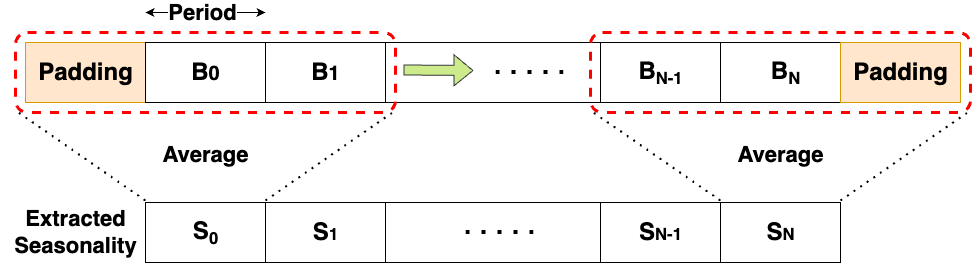
Figure 1: Extracting seasonal patterns using a sliding window of size $l$ and a stride of $m$ times the length of the seasonality period, respectively. In this example, $l{=}3$ and $m{=}1$.

In each step of moving the sliding window, $S_{i}$ is calculated using the following equation:

$$S_{i}=\frac{1}{l}\sum_{j=i}^{i+l-1}B_{i},$$ (2)

where $B_{i}$ is the i-th block of the detrended time-series. Each block is a vector containing $p$ data points, where $p$ represents the length of the seasonality period, ranging from index $i\times p$ to $(i+1)\times p-1$. To preserve the input length, padding is added to both ends of the time-series. This padding consists of repeated copies of the first and last blocks.

Finally, the so-obtained seasonal components are subtracted from the detrended series to obtain the residual component. Each variate of the multivariate time-series, except for date and time features, undergoes this decomposition process separately. By the end of this procedure, we have extracted a trend, a residual, and one or multiple seasonal components for each variate, ensuring that the unique characteristics of each time-series are accurately captured and ready for the subsequent analysis.

4.1.2 Learning graph structure for each component

After decomposing the time-series into its constructing components, we construct the underlying graph for each component by connecting a subset of nodes. To ensure computational efficiency, each component is downsampled to a level that preserves its general patterns.

Next, the distance between two variates is measured using the Dynamic Time Warping (DTW) Müller (2007) metric. DTW is chosen for its robustness in handling nonlinear alignments, providing reliable similarity measurements between time-series. Finally, we connect each node to its $K$ nearest neighbors according to the DTW distance, with $K$ being a hyperparameter in our approach. The described procedure is outlined in Alg. 1.

Algorithm 1 Time-series Graph Construction

0: time-series data $\{X_{i}\}_{i=1}^{D}$, seasonality periods $P_{1},P_{2},...,P_{r}$, number of nearest neighbors K

0: Underlying Graph G

1: Pattern Extraction:

2: for each time-series $X_{i}$ do

3:  Extract trend component $T_{i}$ using a moving weighted average with tricube weights and then downsample

4:  Detrend the series: $\hat{X}_{i}=X_{i}-T_{i}$

5:  Extract seasonality component $S_{i}$

6:  for each seasonality period $P$ in $\{P_{1},P_{2},...,P_{r}\}$ do

7:   Apply a moving aggregation approach with window length $l\times P$ and stride $m\times P$

8:   Compute seasonality component $S_{i}$ as the average of the $n$ periods

9:  end for

10: end for

11: Distance Metric:

12: Use DTW metric to calculate the distance between any two pairs of variates and construct distance matrix $D$ as shown in Fig. 3

13: Construct the Underlying Graph

14: Connect each node to its K nearest neighbors

Fig. 2 depicts the inferred graph from the trend component of the carbon intensity dataset, described in Section 5.1. Here the inferred graph is directional, as one variate might be dependent on the lagged version of the other one, but the opposite is not necessarily true. Fig. 3 illustrates the Dynamic Time Warping (DTW) distances between different nodes for both the trend and seasonal components of the air pollution dataset. These heatmaps reveal distinct patterns of similarity, with lower normalized DTW values indicating stronger temporal alignment between nodes.

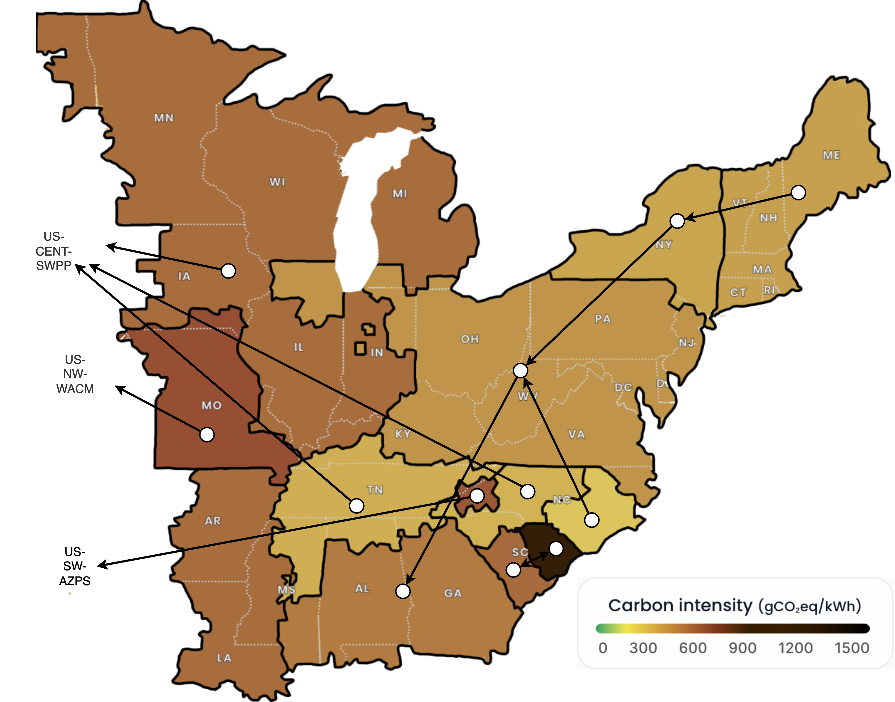
Figure 2: The carbon intensity value is shown for a subset of states in the US at a given point in time. Dark brown (light yellow) indicates higher (lower) carbon intensity in a jurisdiction. Data has been collected from a number of power generation companies, which may supply power to different states. Consequently, the relationship between the states and energy-providing companies is many-to-many. Some arrows extend beyond the map because the image shows only a portion of the full area, and some zones connect to others not included in the display.

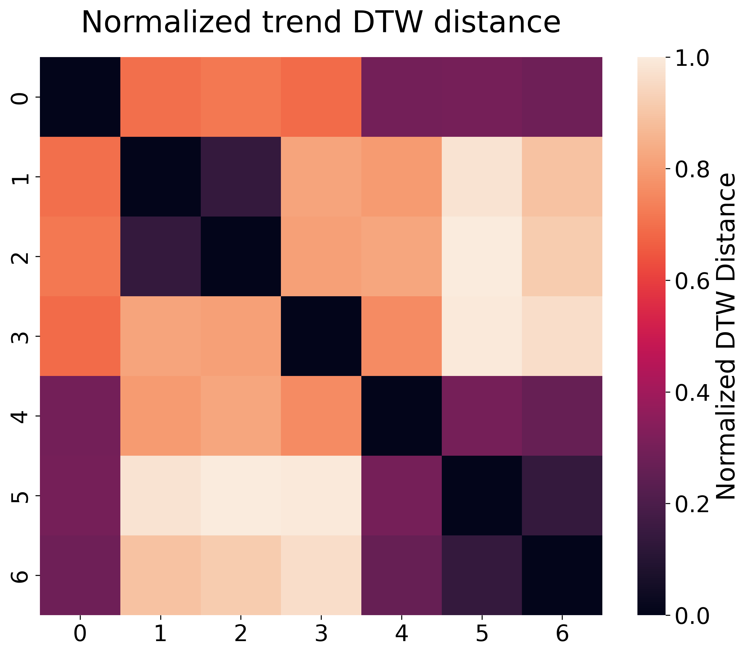
(a)

(b)

Figure 3: Heatmap of DTW distances between different nodes for (a) trend and (b) seasonal components of the air pollution dataset, described in Section 5.1. Note that the distance matrices are symmetrical, with lower values indicating greater closeness. All values are min-max normalized to ensure consistent scaling.

4.2 Spatio-Temporal Forecasting

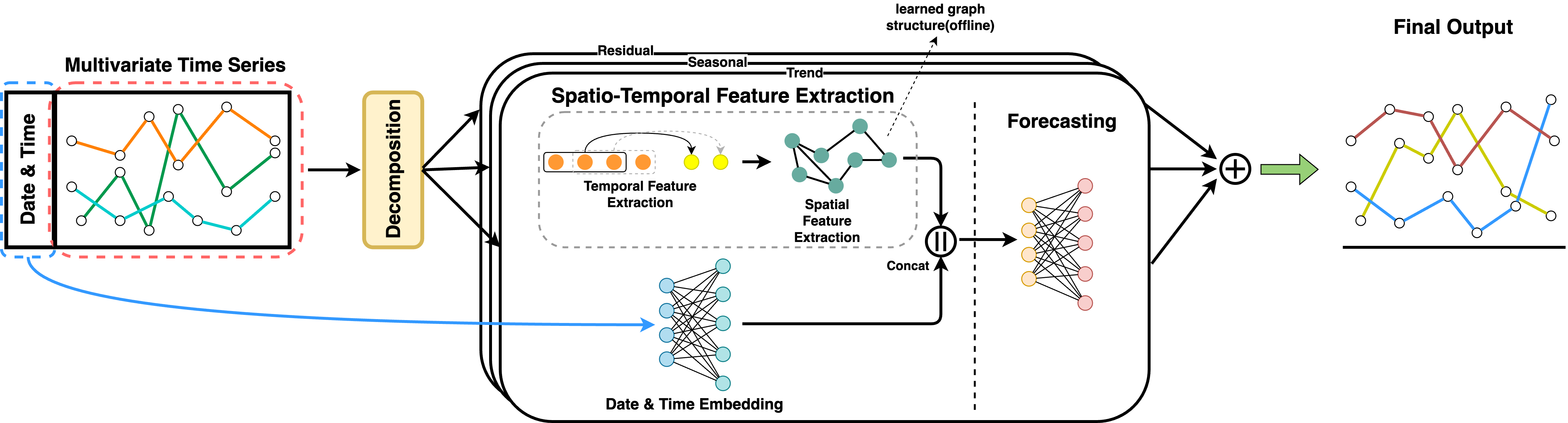
Figure 4: The overall architecture of proposed forecasting model. After decomposition, each component is handled independently.

Now that we have learned the respective graph structure for each constituent component in an offline fashion, as described in Section 4.1.1, we proceed with the spatio-temporal forecasting step. The overall architecture of the proposed forecasting model is illustrated in Fig. 4. The input of the model is a sample of fixed-length historical values. These historical values include date and time features, along with a number of variates that we would like to predict.

4.2.1 Sample Decomposition

Figure 5: Decomposition of an electricity consumption sample over two weeks. The first subplot displays the original data alongside the sum of the trend and seasonal components, showing their closeness.

First, we need to decompose an input sample, without date and time features, into its constituent components: trend, seasonality, and residual. This process follows the procedure described in Section 4.1.1, but without the need for downsampling. Fig. 5 illustrates the decomposition of a randomly selected sample from the Electricity dataset, described in Section 5.1.

4.2.2 Spatial feature extraction

Our feature extraction model handles each component, that is, trend, seasonal, and residual, independently. For each component, we extract and combine three types of features, namely date-time, spatial, and temporal features.

The date-time features are processed through a linear layer to capture some temporal patterns. Simultaneously, spatial and temporal features are extracted from the input data. These temporal and spatial features are then combined and passed on to the forecasting module that uses them to generate the final output. Fig. 6 is a schematic diagram of the feature extraction module.

$$\hat{y}_{t}=f_{\text{forecast}}\left(f_{\text{time}}(x_{\text{time}})\oplus f_{\text{spatio-temporal}}(x)\right)$$ (3)

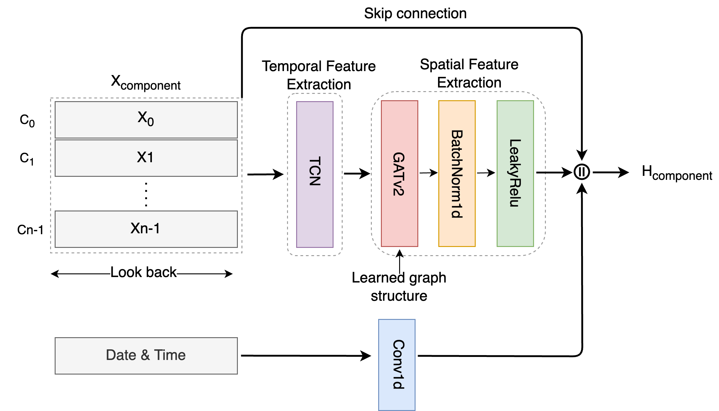
Figure 6: One layer of spatio-temporal feature extraction with time embedding. The input to this module has n channels, $C_{0}$ to $C_{n}-1$. Each component from the decomposition module—trend, seasonal, and residual—is processed independently using this layer. The spatial feature extractor is a Graph Attention Network v2 (GATv2), with a pre-inferred, static underlying graph structure that does not change over time.

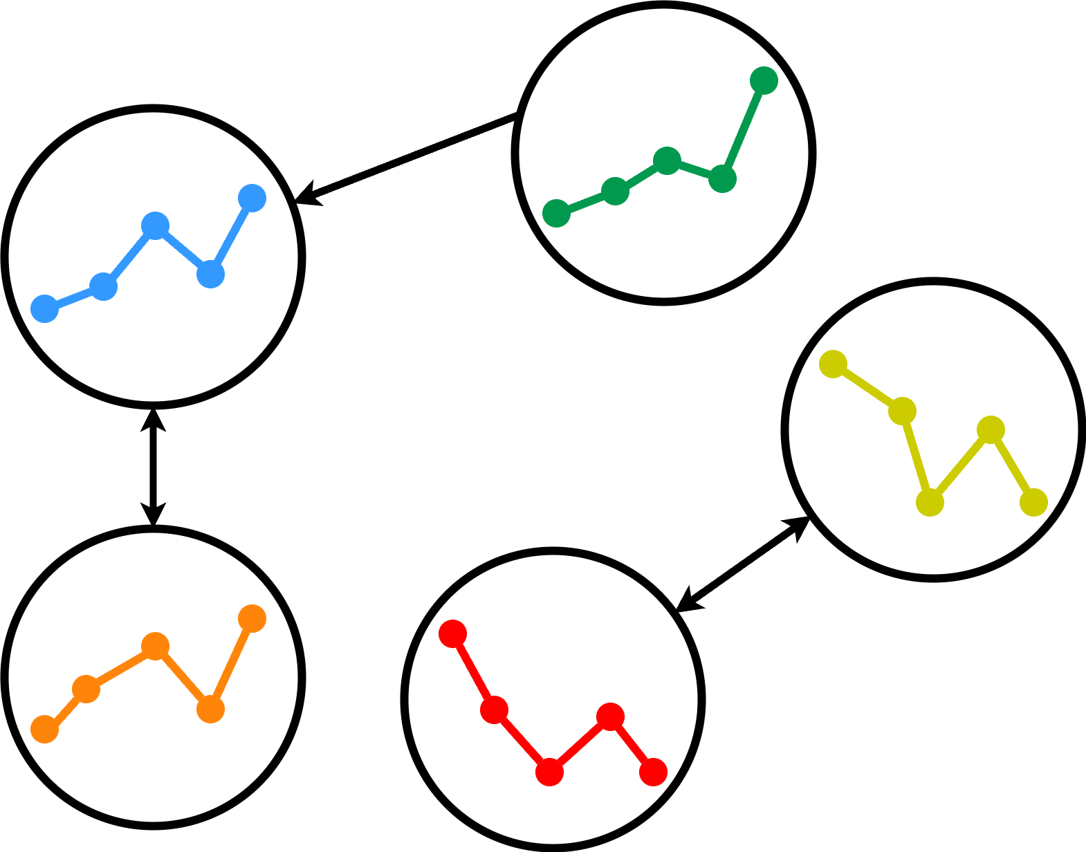
Figure 7: Modeling of multivariate time-series as a graph. Each node represents a variate, and its historical data serves as the features of that node

For spatial feature extraction, we utilize a model based on GATv2 Brody et al. (2021). In this model, each variate of the time-series is treated as a node, with its historical values within the sample serving as its features, as depicted in Fig. 7. GATv2 requires a connection graph to understand the relationships between different nodes (variates). The connection graph is inferred using the method described in Section 4.1.

In a GNN, each node iteratively updates its state by aggregating information from its neighbors. The general formulation of a GNN layer is as follows:

$$\mathbf{h}_{i}^{\prime}=\sigma\left(\mathbf{W}\mathbf{h}_{i}+\sum_{j\in\mathcal{N}_{i}}\mathbf{W}_{j}\mathbf{h}_{j}\right)$$ (4)

where $\mathbf{h}_{i}$ is the feature vector of node $i$, $\mathcal{N}_{i}$ represents the set of neighbors of node $i$, $\mathbf{W}$ and $\mathbf{W}_{j}$ are learnable weight matrices, and $\sigma$ is a nonlinear activation function. This aggregation allows the model to capture the dependencies between nodes and their neighbors, which is crucial for spatial feature extraction.

In GNNs, Equation 4 is used to calculate the updated node representation as a weighted sum of the neighbors’ representation. To increase learning capacity, we can incorporate this method with an attention mechanism. The Graph Attention Network (GAT) Veličković et al. (2017) enhances the GNN framework by incorporating an attention mechanism. This mechanism allows nodes to assign different amounts of importance to the neighbors, which enables capturing of changing dynamics. Specifically, the attention score $e_{ij}$ between node $i$ and its neighbor $j$ is computed as:

$$e_{ij}=\text{LeakyReLU}\left(\mathbf{a}^{T}[\mathbf{W}\mathbf{h}_{i}\parallel\mathbf{W}\mathbf{h}_{j}]\right)$$ (5)

where $\mathbf{a}$ is a learnable weight vector, $\mathbf{W}$ is a weight matrix, $\mathbf{h}_{i}$ and $\mathbf{h}_{j}$ are the feature vectors of nodes $i$ and $j$, respectively, and $\parallel$ denotes concatenation. The attention scores are then normalized using Softmax:

$$\alpha_{ij}=\text{softmax}_{j}(e_{ij})=\frac{\exp(e_{ij})}{\sum_{k\in\mathcal{N}_{i}}\exp(e_{ik})}$$ (6)

The final output representation of node $i$ is computed as a weighted sum of its neighbors’ features:

$$\mathbf{h}_{i}^{\prime}=\sigma\left(\sum_{j\in\mathcal{N}_{i}}\alpha_{ij}\mathbf{W}\mathbf{h}_{j}\right)$$ (7)

This attention mechanism allows GAT to focus on the most relevant neighbors, improving its ability to capture complex relationships in the graph.

GATv2 Brody et al. (2021), builds on the original GAT by addressing its limitations and introducing a more expressive dynamic attention mechanism. In GATv2, the attention score computation is modified to condition both the query and key nodes, enhancing the model’s flexibility. The new attention score $e_{ij}$ is defined as:

$$e_{ij}=\mathbf{a}^{T}\text{LeakyReLU}\left(\mathbf{W}[\mathbf{h}_{i}\parallel\mathbf{h}_{j}]\right)$$ (8)

In this architecture, we employed just one layer of GATv2. The decision of whether to use one layer of GATv2 or stack more of them has been made empirically. Fig. 9 in Appendix A justifies why one layer of the GATv2 layer was employed for the carbon intensity dataset.

4.2.3 Temporal Feature Extraction

For temporal feature extraction, we utilize Temporal Convolutional Networks (TCNs) Bai et al. (2018). TCNs are designed to capture temporal dependencies in sequential data by leveraging convolution across time steps. The key components of TCNs are causal convolutions, dilations, and residual connections.

Causal convolutions ensure that the model only uses past information to predict future values, preserving the temporal order of the data. The causal convolution for a given layer $l$ is defined as:

$$\mathbf{y}_{t}^{l}=\sum_{i=0}^{k-1}\mathbf{W}_{i}^{l}\mathbf{x}_{t-i}$$ (9)

where $\mathbf{y}_{t}^{l}$ is the output at time $t$ for layer $l$, $\mathbf{W}_{i}^{l}$ are the convolutional filters, $\mathbf{x}_{t-i}$ are the inputs from the previous layer, and $k$ is the filter size.

Dilated convolutions expand the receptive field of the network without increasing the number of parameters, allowing the model to capture long-range dependencies. The dilation factor $d$ determines the spacing between the kernel elements. A dilated convolution is defined as:

$$\mathbf{y}_{t}^{l}=\sum_{i=0}^{k-1}\mathbf{W}_{i}^{l}\mathbf{x}_{t-i\cdot d}$$ (10)

where $d$ is the dilation factor, $k$ is the filter size, and the other symbols retain their previous meanings.

Residual connections help mitigate the vanishing gradient problem and facilitate the training of deeper networks. The output of each TCN layer is combined with its input through a residual connection:

$$\mathbf{y}_{t}=\sigma\left(\mathbf{y}_{t}^{l}+\mathbf{x}_{t}\right)$$ (11)

4.2.4 Forecasting

Once features are extracted for each component of the time-series, we employ a linear forecasting model to produce forecasts for the entire forecast horizon at once, utilizing a direct multistep forecasting approach. This choice is motivated by the demonstrated effectiveness of similar methods in previous studies Sohrabbeig et al. (2023); Zeng et al. (2023). Forecasts are generated simultaneously and independently for each component—trend, seasonal, and residual—mirroring the approach used in the feature extraction phase. Within each forecasting component, each variate is forecasted in a univariate fashion. This means that only the spatial and temporal features extracted for each specific variate in the previous step are used for forecasting that variate. Nevertheless, these features are influenced by the features of some other variates due to the way that they are generated.

The input to the forecasting module is the combination of spatio-temporal features and time embeddings. In this work, these features and embeddings are added together before being fed into the forecasting task. The decision to add rather than concatenate the time embeddings with the other extracted features was made based on our experimental results. Fig. 6 shows the input for the forecasting module.

The linear forecasting model operates on input data with the following characteristics:

• Input Sequence Length ($L$): The length of the input time-series sequence.

• Prediction Length ($H$): The number of future time steps to be predicted.

• Number of Channels ($D$): The number of separate time-series channels in the input data.

The input to the model is a tensor $\mathbf{X}$ of shape $(B,D,L)$, where $B$ is the batch size, $D$ is the number of channels, and $L$ is the length of the input sequence. During the forward pass, the model computes the prediction $\mathbf{Y}$ using the input tensor $\mathbf{X}$ and the learnable parameters. This is done through a linear transformation followed by the addition of the bias term:

$$\mathbf{Y}=\mathbf{W}\cdot\mathbf{X}+\mathbf{b}$$ (12)

where $\mathbf{Y}=\mathbf{W}\cdot\mathbf{X}$ represents the Einstein summation operation defined as:

$$\mathbf{Y}_{bdh}=\sum_{l=1}^{L}\mathbf{W}_{dhl}\cdot\mathbf{X}_{bdl}$$ (13)

for each batch $b$, channel $d$, and prediction time step $h$. This process allows the model to learn a linear mapping from the input sequence to the predicted sequence, leveraging the entire input sequence to inform each prediction step. This implementation is more efficient than the method used by DLinear and NLinear Zeng et al. (2023) models, which iteratively calculates forecasts for each variate.

5 Result

In this section, we first introduce the datasets and baseline models used for evaluation, then evaluate and compare the performance of our proposed model with the baselines in three different settings.

5.1 Datasets

For comprehensive coverage of critical factors influencing time series data, we select four urban datasets including electricity usage, weather conditions, carbon intensity, and air pollution. These datasets provide a robust benchmark for understanding the pros and cons of different time series forecasting models. More details on these datasets are provided below:

• Electricity: This dataset contains hourly electricity consumption of 321 customers over three years.

• Weather: This dataset contains a meteorological series with 21 weather metrics collected every ten minutes in 2020, from a weather station at the Max Planck Biogeochemistry Institute.

• Carbon intensity: This dataset contains hourly measurements of carbon intensity in 50 states and four territories in the US. The data was collected over three years.

• Air pollution: This dataset provides hourly PM2.5 measurements recorded by the US Embassy in Beijing Liang et al. (2015). Additionally, it includes meteorological data collected from Beijing Capital International Airport.

Table 1 summarizes all the main characteristics of the above datasets. With the exception of the air pollution dataset, the other datasets did not require any imputation of missing values. For the air pollution dataset, missing values were filled using the average of records corresponding to the same month, day of the week, and hour. As a preprocessing step, all columns in all datasets were standardized.

Table 1: Statistical details of the real-world datasets used in this study.

Dataset	No. Features	Length	Time Resolution
Electricity	321	26,304	1h
Air Pollution	7	34,970	1h
Carbon	54	26,280	1h
Weather	21	52,696	10min

5.2 Baselines

To evaluate our model, we use three highly effective Transformer models, namely Informer Zhou et al. (2021), Autoformer Wu et al. (2021), and FEDformer Zhou et al. (2022), as our baselines. Additionally, we consider two recent state-of-the-art models, NLinear and DLinear Zeng et al. (2023). We also employed a straightforward baseline: Repeat Last, which replicates the last observation. Our next baseline is TimesFM Das et al. (2023), a foundation model for time series forecasting that leverages a decoder-only attention mechanism with input patching. TimesFM is pre-trained on a large corpus of both real-world and synthetic time series data, enabling it to achieve near state-of-the-art zero-shot performance across various datasets without the need for fine-tuning. In these experiments, TimesFM was used solely for inference and was not fine-tuned.

In this study, we did not compare our results with classical models such as ARIMA and SARIMA, due to the extensive time required for their parameter selection, which significantly slows down the training process. Instead, we based our conclusions on experimental results reported in other studies Wu et al. (2021); Zhou et al. (2021), which have shown that these classical models perform poorly on the long sequence time series forecasting (LSTF) task. Therefore, we opted not to include them in our direct comparisons.

5.3 Experiments

We now evaluate the performance of our model (labelled DST in the tables) and compare it with strong baselines in three different settings. In all experiments, the length of the look-back window is 336, and the learning rate is set to 0.0001. The length of the forecast horizon is denoted in the second column of tables˜2, 3 and 4. For our model, we decided to extract only one seasonal component due to the short length of the input. For instance, when the length of the look-back window is 336 hours (equivalent to two weeks), it is logical to extract daily seasonal patterns since multiple daily cycles are present in this period while extracting weekly patterns would be less meaningful considering the limited number of weekly cycles.

Dataset Length DST DLinear NLinear Autoformer TimesFM Repeat Last IMP MSE MAE MSE MAE MSE MAE MSE MAE MSE MAE MSE MAE MSE MAE Air pollution 96 0.402 0.322 0.421 0.324 0.441 0.334 0.481 0.382 0.532 0.429 0.745 0.589 4.51 0.62 192 0.422 0.333 0.439 0.340 0.447 0.344 0.483 0.376 0.535 0.431 0.813 0.615 3.87 2.06 336 0.427 0.341 0.447 0.350 0.467 0.358 0.488 0.382 0.542 0.431 0.804 0.623 4.47 2.57 720 0.423 0.347 0.469 0.375 0.472 0.379 0.452 0.342 0.549 0.432 0.827 0.644 9.80 7.46 Carbon 96 0.468 0.501 0.476 0.503 0.467 0.492 0.512 0.539 0.519 0.547 1.128 0.780 -0.21 -1.83 192 0.534 0.545 0.541 0.544 0.540 0.547 0.674 0.621 0.584 0.580 1.243 0.829 1.11 0.37 336 0.589 0.581 0.601 0.595 0.597 0.594 0.703 0.659 0.631 0.629 1.328 0.865 1.34 2.19 720 0.721 0.656 0.731 0.669 0.729 0.661 0.878 0.738 0.723 0.650 1.489 0.927 1.10 0.76 Electricity 96 0.131 0.228 0.149 0.252 0.136 0.232 0.190 0.301 0.189 0.298 1.528 0.927 3.68 1.72 192 0.141 0.241 0.160 0.264 0.167 0.269 0.202 0.313 0.204 0.311 1.521 0.927 11.87 8.71 336 0.153 0.260 0.170 0.279 0.169 0.275 0.210 0.318 0.231 0.336 1.530 0.934 9.47 5.45 720 0.171 0.282 0.204 0.314 0.200 0.298 0.239 0.350 0.246 0.361 1.535 0.942 14.5 5.37 Weather 96 0.178 0.261 0.169 0.251 0.175 0.259 0.364 0.406 0.319 0.329 0.258 0.254 -5.33 -3.98 192 0.234 0.315 0.229 0.300 0.225 0.299 0.436 0.439 0.322 0.354 0.339 0.294 -4.00 -7.14 336 0.381 0.443 0.321 0.403 0.352 0.412 0.470 0.469 0.401 0.391 0.421 0.343 -18.69 -29.15 720 0.549 0.536 0.414 0.465 0.421 0.481 0.467 0.447 0.433 0.444 0.465 0.394 -32.60 -36.04

Table 2: Experimental results on real data in multivariate input, multivariate output setting. The results were averaged over five runs to eliminate the effect of randomness. The IMP column displays the error reduction of our proposed model compared to the best baseline. The best results are highlighted in bold and the second-best results are in underlined.

Dataset Length DST DLinear NLinear Autoformer TimesFM Repeat Last IMP MSE MAE MSE MAE MSE MAE MSE MAE MSE MAE MSE MAE MSE MAE Air pollution 96 0.864 0.703 0.874 0.699 0.872 0.701 0.947 0.714 0.914 0.695 1.579 0.869 0.92 -0.57 192 0.903 0.719 0.926 0.728 0.931 0.732 1.008 0.744 0.973 0.739 1.725 0.926 2.48 1.24 336 0.916 0.722 0.954 0.738 0.955 0.745 1.057 0.792 0.969 0.744 1.799 0.948 3.98 2.17 720 0.945 0.735 0.986 0.746 1.015 0.783 1.063 0.814 1.009 0.751 1.877 0.977 4.16 1.47 Carbon 96 0.232 0.370 0.235 0.375 0.244 0.381 0.731 0.858 0.418 0.561 1.771 1.039 1.28 1.33 192 0.248 0.389 0.273 0.406 0.284 0.412 0.779 0.871 0.445 0.594 1.853 1.077 9.16 4.19 336 0.266 0.410 0.307 0.430 0.305 0.427 0.801 0.896 0.457 0.612 1.919 1.106 12.79 3.98 720 0.282 0.425 0.368 0.476 0.364 0.469 0.818 0.914 0.551 0.687 2.025 1.141 22.53 9.38 Electricity 96 0.148 0.273 0.166 0.292 0.169 0.293 0.194 0.309 0.200 0.291 1.221 0.858 10.84 6.19 192 0.176 0.298 0.189 0.312 0.191 0.320 0.211 0.319 0.209 0.319 1.223 0.857 6.87 4.49 336 0.188 0.310 0.209 0.329 0.204 0.321 0.218 0.330 0.211 0.334 1.297 0.881 7.84 3.43 720 0.214 0.335 0.252 0.371 0.255 0.374 0.240 0.351 0.258 0.359 1.369 0.908 10.83 4.56 Weather 96 0.096 0.206 0.127 0.234 0.131 0.237 0.109 0.212 0.112 0.243 0.130 0.262 11.93 2.83 192 0.378 0.416 0.412 0.425 0.423 0.427 0.401 0.419 0.439 0.461 0.451 0.478 5.74 0.72 336 0.780 0.604 0.834 0.613 0.845 0.621 0.806 0.605 0.812 0.604 0.844 0.620 3.23 0.00 720 1.237 0.797 1.408 0.825 1.392 0.818 1.398 0.816 1.418 0.876 1.470 0.934 11.14 2.33

Table 3: Experimental results on real data in multivariate input, univariate output setting. The results were averaged over five runs to eliminate the effect of randomness. The IMP column displays the error reduction of our proposed model compared to the best baseline. The best results are highlighted in bold and the second-best results are in underlined.

Dataset Length DST DLinear NLinear Autoformer TimesFM Repeat Last IMP MSE MAE MSE MAE MSE MAE MSE MAE MSE MAE MSE MAE MSE MAE Air pollution 96 0.867 0.695 0.874 0.699 0.872 0.701 0.961 0.732 0.917 0.699 1.579 0.869 0.57 0.57 192 0.921 0.724 0.926 0.728 0.931 0.732 1.023 0.760 0.971 0.741 1.725 0.926 0.54 0.55 336 0.950 0.736 0.954 0.738 0.955 0.745 1.084 0.803 1.001 0.747 1.799 0.948 0.42 0.27 720 0.984 0.747 0.986 0.746 1.015 0.783 1.092 0.833 1.013 0.755 1.877 0.977 0.20 -0.13 Carbon 96 0.216 0.357 0.235 0.375 0.244 0.381 0.615 0.796 0.422 0.567 1.771 1.039 8.08 4.80 192 0.264 0.398 0.273 0.406 0.284 0.412 0.631 0.818 0.446 0.601 1.853 1.077 3.29 1.97 336 0.293 0.422 0.307 0.430 0.305 0.427 0.722 0.846 0.463 0.615 1.919 1.106 3.3 1.17 720 0.360 0.471 0.368 0.476 0.364 0.469 0.779 0.875 0.557 0.690 2.025 1.141 1.10 -0.42 Electricity 96 0.154 0.277 0.166 0.292 0.169 0.293 0.198 0.311 0.209 0.291 1.221 0.858 7.23 4.81 192 0.173 0.297 0.189 0.312 0.191 0.320 0.214 0.323 0.223 0.342 1.223 0.857 8.46 4.81 336 0.196 0.315 0.209 0.329 0.204 0.321 0.231 0.348 0.231 0.345 1.297 0.881 3.92 1.87 720 0.238 0.357 0.252 0.371 0.255 0.374 0.288 0.389 0.307 0.398 1.369 0.908 5.55 3.77 Weather 96 0.119 0.228 0.127 0.234 0.131 0.237 0.138 0.245 0.157 0.282 0.130 0.262 6.30 2.56 192 0.421 0.433 0.412 0.425 0.423 0.427 0.476 0.501 0.470 0.483 0.451 0.478 -2.18 -1.88 336 0.843 0.621 0.834 0.613 0.845 0.621 0.864 0.658 0.872 0.684 0.844 0.620 -1.07 -1.30 720 1.414 0.826 1.408 0.825 1.392 0.818 1.412 0.835 1.555 0.954 1.470 0.934 -1.58 -0.97

Table 4: Experimental results on real data in univariate input, univariate output. The results were averaged over five runs to eliminate the effect of randomness. The IMP column displays the error reduction of our proposed model compared to the best baseline. The best results are highlighted in bold and the second-best results are in underlined.

As shown in Tables 2, 3, and 4, our proposed model has achieved the best or near-best results across all settings. We present detailed results in three different settings to ensure a fair comparison of the strengths and weaknesses of the baseline models and to clearly explain the effectiveness of our proposed model.

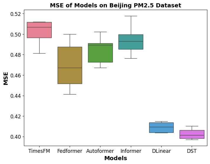
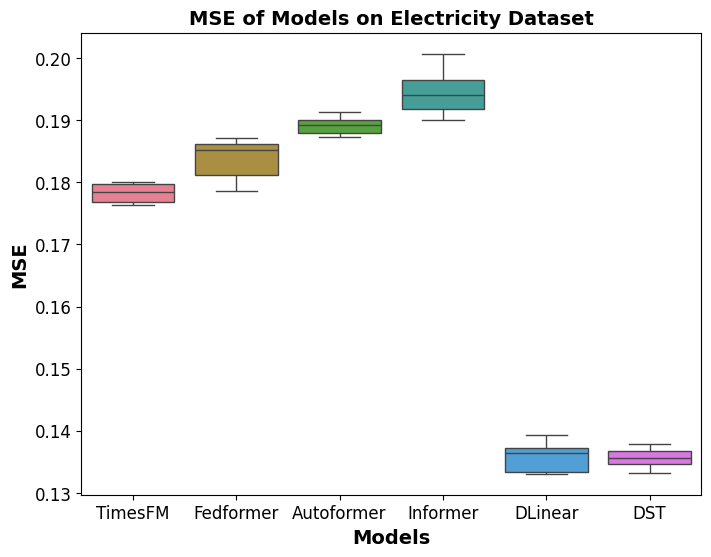
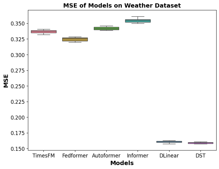
Figure 8: MSE comparison of our proposed model against baselines on different datasets. This is a multivariate input, multivariate output task, with input and output lengths of 336 and 96, respectively. Note that the axis scales are exaggerated for better visualization of the differences between models.

DLinear and NLinear achieve the best performance among the baselines. Despite their impressive performance, they are univariate models that lack a mechanism to extract spatial dependencies. This limitation becomes evident in the multivariate input and univariate forecasting setting, where forecasting a variate may benefit from capturing lagged dependencies with other variates. Univariate models like DLinear or NLinear cannot leverage this information, leading to inferior performance compared to models that can, such as our proposed model and transformer-based models. This is particularly evident in the forecasting of PM2.5 with multivariate input.

Transformer-based forecasting models, such as Autoformer, Fedformer, and Informer, are highly complex and over-parameterized, making them susceptible to overfitting. This issue is apparent in the forecasting of the carbon dataset. Additionally, we have included the inference results of TimesFM, which were obtained without additional training or fine-tuning. This lack of fine-tuning likely contributes to its suboptimal performance, as it might not have adapted well to the specific characteristics of the datasets. Pretrained models are generally not tailored to the nuances of new datasets unless they undergo further training to update their parameters. Consequently, the model’s inability to learn and adjust to the unique temporal patterns and data distribution of the datasets has likely resulted in less accurate forecasts compared to the other models that were specifically trained.

Figure 8 presents a comparative analysis of the Mean Squared Error (MSE) performance of our proposed model, DST, against several baseline models across four datasets: Beijing PM2.5, Carbon, Electricity, and Weather. This evaluation is conducted on a multivariate input-multivariate output forecasting task, where the input and output lengths are set to 336 and 96, respectively. The results demonstrate that DST consistently achieves lower MSE values compared to the baselines, indicating its superior forecasting capability. Notably, traditional transformer-based models, such as Autoformer and Informer, tend to exhibit higher variance and median errors, suggesting increased instability in their predictions. DLinear, a linear baseline, performs competitively but is outperformed by DST, particularly on the Carbon dataset. The y-axis scales are adjusted for better visualization of performance differences among the models

6 Ablations

To thoroughly examine the properties of our proposed model, we conducted ablation studies to evaluate the effectiveness of each of its key modules. The modules under evaluation include (1) Decomposition, (2) Date and Time Embedding, (3) Temporal Feature Extraction, and (4) Spatial Feature Extraction. For each dataset, we compare the model’s performance with and without each of these modules.

Due to the modular and pipelined structure of the proposed architecture, we can easily remove individual modules without impacting the functionality of the remaining components. The only exception is the Date and Time Embedding module, whose output is concatenated with the extracted spatio-temporal features. To simulate the removal of this module, we replace its output with zero-vectors, thereby mitigating its effect on the model’s performance.

Table 5 demonstrates the effectiveness of each module within the model architecture. Among all the components, the temporal feature extraction module plays the most influential role, as indicated by the highest increase in Mean Squared Error (MSE) when this module is removed. This suggests that capturing temporal dependencies is crucial for accurately modeling the datasets, particularly for data characterized by strong temporal patterns, such as air pollution, carbon emissions, and electricity usage. The ablation results also reveal that other modules, such as decomposition, date and time embedding, and spatial feature engineering, contribute significantly to model performance, albeit to a lesser extent. These components work synergistically to enhance predictive accuracy by providing complementary information that captures different aspects of the data, such as spatial correlations and temporal variations. Overall, the study reveals the necessity of taking a multi-faceted approach that integrates various techniques to effectively handle complex, real-world datasets.

Additionally, we conducted experiments to evaluate the impact of the number of GATv2 layers. Across all experiments, a single layer for spatial feature extraction consistently yielded the best performance. Figure 9 illustrates how the MSE changes as more GATv2 layers are added for the carbon intensity dataset.

Dataset	Air Pollution	Carbon	Electricity	Weather
w/o Decomposition	0.441	0.474	0.154	0.179
w/o Date&Time Emb.	0.424	0.482	0.149	0.158
w/o Temporal F.E.	0.452	0.491	0.162	0.161
w/o Spatial F.E.	0.439	0.488	0.156	0.165
Original	0.404	0.460	0.133	0.155

Table 5: Ablation studies on the effectiveness of key modules. Reported values are the MSE of each setting.

7 Conclusion

In this paper, we introduced a novel multivariate time-series forecasting model that leverages the advanced capabilities of GATv2 to capture spatial dependencies among different time-series variables. Our approach, which incorporates a decomposition-based preprocessing step, has demonstrated incremental improvements in forecast accuracy and reliability across various real-world datasets. The experimental results underscore the potential of our model to outperform existing state-of-the-art methods, particularly in complex domains such as energy management, weather prediction, carbon intensity forecasting, and air pollution monitoring. By effectively modeling the intricate interdependencies within multivariate time-series data, our proposed model provides a robust framework for long-term forecasting, contributing to the development of smart infrastructure systems and enhancing societal outcomes. Future work will focus on further optimizing the model, exploring its applicability to additional domains, and integrating adaptive graph learning techniques to enhance its performance in dynamic environments.

Appendix

Appendix A Number of GATv2 layers

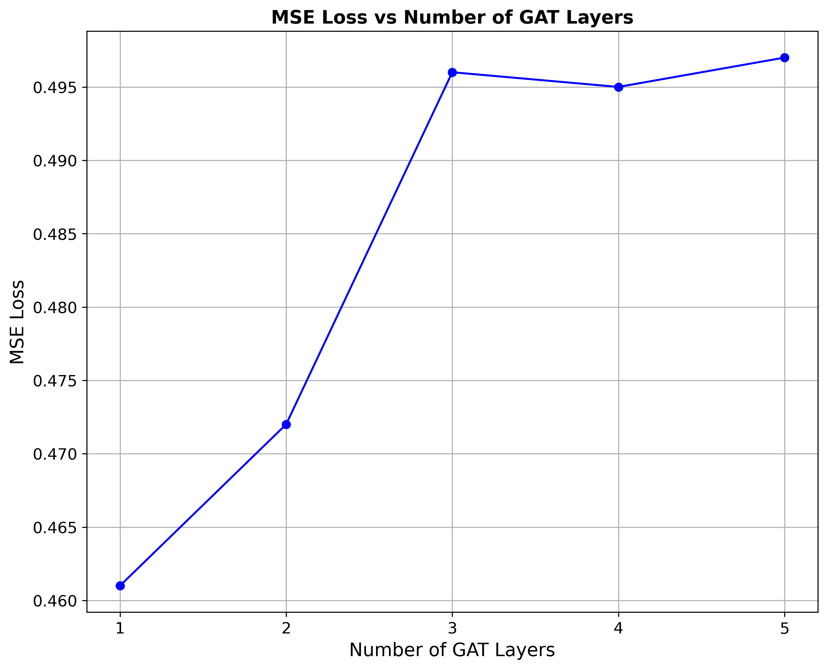
Figure 9: Changes of MSE loss by increasing the number of GATv2 layers used for spatial feature extraction on carbon intensity dataset.

References

- Nti et al. [2020] Isaac Kofi Nti, Moses Teimeh, Owusu Nyarko-Boateng, and Adebayo Felix Adekoya. Electricity load forecasting: a systematic review. Journal of Electrical Systems and Information Technology, 7:1–19, 2020.
- Huang et al. [2021] Guoyan Huang, Xinyi Li, Bing Zhang, and Jiadong Ren. Pm2. 5 concentration forecasting at surface monitoring sites using gru neural network based on empirical mode decomposition. Science of the Total Environment, 768:144516, 2021.
- Du et al. [2024] Shangjie Du, ZhiZhang Hu, and Shijia Pan. Graphy: Graph-based physics-guided urban air quality modeling for monitoring-constrained regions. In Proceedings of the 11th ACM International Conference on Systems for Energy-Efficient Buildings, Cities, and Transportation, pages 33–43, 2024.
- Mouatadid et al. [2024] Soukayna Mouatadid, Paulo Orenstein, Genevieve Flaspohler, Miruna Oprescu, Judah Cohen, Franklyn Wang, Sean Knight, Maria Geogdzhayeva, Sam Levang, Ernest Fraenkel, et al. Subseasonalclimateusa: a dataset for subseasonal forecasting and benchmarking. Advances in Neural Information Processing Systems, 36, 2024.
- Maji et al. [2022] Diptyaroop Maji, Prashant Shenoy, and Ramesh K Sitaraman. Carboncast: multi-day forecasting of grid carbon intensity. In Proceedings of the 9th ACM International Conference on Systems for Energy-Efficient Buildings, Cities, and Transportation, pages 198–207, 2022.
- Wu et al. [2020] Zonghan Wu, Shirui Pan, Guodong Long, Jing Jiang, Xiaojun Chang, and Chengqi Zhang. Connecting the dots: Multivariate time series forecasting with graph neural networks. In Proceedings of the 26th ACM SIGKDD international conference on knowledge discovery & data mining, pages 753–763, 2020.
- Veličković et al. [2017] Petar Veličković, Guillem Cucurull, Arantxa Casanova, Adriana Romero, Pietro Lio, and Yoshua Bengio. Graph attention networks. arXiv preprint arXiv:1710.10903, 2017.
- Brody et al. [2021] Shaked Brody, Uri Alon, and Eran Yahav. How attentive are graph attention networks? arXiv preprint arXiv:2105.14491, 2021.
- Bai et al. [2018] Shaojie Bai, J Zico Kolter, and Vladlen Koltun. An empirical evaluation of generic convolutional and recurrent networks for sequence modeling. arXiv preprint arXiv:1803.01271, 2018.
- Radovanović et al. [2023] Ana Radovanović et al. Carbon-aware computing for datacenters. IEEE Transactions on Power Systems, 38(2):1270–1280, 2023.
- Box and Jenkins [1968] George EP Box and Gwilym M Jenkins. Some recent advances in forecasting and control. Journal of the Royal Statistical Society. Series C (Applied Statistics), 17(2):91–109, 1968.
- Box and Pierce [1970] George EP Box and David A Pierce. Distribution of residual autocorrelations in autoregressive-integrated moving average time series models. Journal of the American statistical Association, 65(332):1509–1526, 1970.
- Holt [2004] Charles C Holt. Forecasting seasonals and trends by exponentially weighted moving averages. International journal of forecasting, 20(1):5–10, 2004.
- Winters [1960] Peter R Winters. Forecasting sales by exponentially weighted moving averages. Management science, 6(3):324–342, 1960.
- Boser et al. [1992] Bernhard E Boser, Isabelle M Guyon, and Vladimir N Vapnik. A training algorithm for optimal margin classifiers. In Proceedings of the fifth annual workshop on Computational learning theory, pages 144–152, 1992.
- Breiman [2001] Leo Breiman. Random forests. Machine learning, 45:5–32, 2001.
- Friedman [2001] Jerome H Friedman. Greedy function approximation: a gradient boosting machine. Annals of statistics, pages 1189–1232, 2001.
- Chen and Guestrin [2016] Tianqi Chen and Carlos Guestrin. Xgboost: A scalable tree boosting system. In Proceedings of the 22nd acm sigkdd international conference on knowledge discovery and data mining, pages 785–794, 2016.
- Hochreiter and Schmidhuber [1997] Sepp Hochreiter and Jürgen Schmidhuber. Long short-term memory. Neural computation, 9(8):1735–1780, 1997.
- Chung et al. [2014] Junyoung Chung, Caglar Gulcehre, Kyunghyun Cho, and Yoshua Bengio. Empirical evaluation of gated recurrent neural networks on sequence modeling. In NIPS 2014 Workshop on Deep Learning, December 2014, 2014.
- Oreshkin et al. [2019] Boris N Oreshkin, Dmitri Carpov, Nicolas Chapados, and Yoshua Bengio. N-beats: Neural basis expansion analysis for interpretable time series forecasting. arXiv preprint arXiv:1905.10437, 2019.
- Zhou et al. [2021] Haoyi Zhou, Shanghang Zhang, Jieqi Peng, Shuai Zhang, Jianxin Li, Hui Xiong, and Wancai Zhang. Informer: Beyond efficient transformer for long sequence time-series forecasting. In Proceedings of the AAAI conference on artificial intelligence, volume 35, pages 11106–11115, 2021.
- Wu et al. [2021] Haixu Wu, Jiehui Xu, Jianmin Wang, and Mingsheng Long. Autoformer: Decomposition transformers with auto-correlation for long-term series forecasting. Advances in Neural Information Processing Systems, 34:22419–22430, 2021.
- Zhou et al. [2022] Tian Zhou, Ziqing Ma, Qingsong Wen, Xue Wang, Liang Sun, and Rong Jin. Fedformer: Frequency enhanced decomposed transformer for long-term series forecasting. In International Conference on Machine Learning, pages 27268–27286. PMLR, 2022.
- Zeng et al. [2023] Ailing Zeng, Muxi Chen, Lei Zhang, and Qiang Xu. Are transformers effective for time series forecasting? In Proceedings of the AAAI conference on artificial intelligence, volume 37, pages 11121–11128, 2023.
- Lin et al. [2024] Shengsheng Lin, Weiwei Lin, Xinyi HU, Wentai Wu, Ruichao Mo, and Haocheng Zhong. Cyclenet: Enhancing time series forecasting through modeling periodic patterns. In The Thirty-eighth Annual Conference on Neural Information Processing Systems, 2024. URL https://openreview.net/forum?id=clBiQUgj4w.
- Jin et al. [2022] Ming Jin, Yu Zheng, Yuan-Fang Li, Siheng Chen, Bin Yang, and Shirui Pan. Multivariate time series forecasting with dynamic graph neural odes. IEEE Transactions on Knowledge and Data Engineering, 35(9):9168–9180, 2022.
- Zhang et al. [2020] Yuxuan Zhang, Yuanxiang Li, Xian Wei, and Lei Jia. Adaptive spatio-temporal graph convolutional neural network for remaining useful life estimation. In 2020 International Joint Conference on Neural Networks (IJCNN), pages 1–7, 2020. doi:10.1109/IJCNN48605.2020.9206739.
- Li and Zhu [2021] Mengzhang Li and Zhanxing Zhu. Spatial-temporal fusion graph neural networks for traffic flow forecasting, 2021. URL https://arxiv.org/abs/2012.09641.
- Kumar et al. [2024] Rahul Kumar, Manish Bhanu, João Mendes-Moreira, and Joydeep Chandra. Spatio-temporal predictive modeling techniques for different domains: a survey. ACM Comput. Surv., 57(2), October 2024. ISSN 0360-0300. doi:10.1145/3696661. URL https://doi.org/10.1145/3696661.
- Das et al. [2023] Abhimanyu Das, Weihao Kong, Rajat Sen, and Yichen Zhou. A decoder-only foundation model for time-series forecasting. arXiv preprint arXiv:2310.10688, 2023.
- Woo et al. [2024] Gerald Woo, Chenghao Liu, Akshat Kumar, Caiming Xiong, Silvio Savarese, and Doyen Sahoo. Unified training of universal time series forecasting transformers. In Proceedings of the 41st International Conference on Machine Learning, ICML’24. JMLR.org, 2024.
- Sohrabbeig et al. [2023] Amirhossein Sohrabbeig, Omid Ardakanian, and Petr Musilek. Decompose and conquer: Time series forecasting with multiseasonal trend decomposition using loess. Forecasting, 5(4):684–696, 2023. ISSN 2571-9394. doi:10.3390/forecast5040037. URL https://www.mdpi.com/2571-9394/5/4/37.
- Müller [2007] Meinard Müller. Dynamic time warping. Information retrieval for music and motion, pages 69–84, 2007.
- Liang et al. [2015] Xuan Liang, Tao Zou, Bin Guo, Shuo Li, Haozhe Zhang, Shuyi Zhang, Hui Huang, and Song Xi Chen. Assessing beijing’s pm2.5 pollution: severity, weather impact, apec and winter heating. Proceedings of the Royal Society A: Mathematical, Physical and Engineering Sciences, 471, 2015. URL https://api.semanticscholar.org/CorpusID:130615236.